real-time air quality measurements using mobile …
TRANSCRIPT

REAL-TIME AIR QUALITY MEASUREMENTS USING MOBILE PLATFORMS
BY PARVEEN SEVUSU
A thesis submitted to the
Graduate School—New Brunswick
Rutgers, the State University of New Jersey
In partial fulfillment of the requirements
For the degree of
Master of Science
Graduate Program in Computer Science
Written under the direction of
Liviu Iftode
And approved by
New Brunswick, New Jersey Jan, 2015

ii
ABSTRACT OF THE THESIS
Real-time Air Quality Measurements Using Mobile Platforms
By PARVEEN SEVUSU
Thesis Director: Liviu Iftode
Air pollution poses a serious threat to our health and quality of life. Measuring pollution in
the air we breathe and sharing the results with our peers is an important step in increasing social
awareness for creating a clean environment. Usually, pollution measurements are conducted using
expensive monitors at fixed locations. These measurements fail to provide accurate real-time
pollution information in most of the highly polluted roads. It is desirable to have access to real time
fine-grained measurements to be able to quickly analyze and identify alarming levels of pollutants.
Pervasiveness of smart phones with internet connectivity and increased availability of
personal air quality sensors provide a unique opportunity to develop air pollution conscious
community of users for collecting and sharing real time air pollution data. In this thesis, we propose
air quality monitoring through mobile sensors, which are low-power, low-cost, designed to sample
air pollutants such as carbon mono-oxide, nitrogen oxide, sulphur dioxide, environmental
temperature, humidity and air pressure and communicate via Bluetooth with a smartphone. We
built an iOS mobile application that makes use of location services available on the mobile phones,
to record GPS co-ordinates along with air pollution readings. We built a mobile to cloud replication
model, data exchange protocol and outlier detection for anomalous sensor readings. We also
employed spatial database queries to optimize location based pollution data sharing and
visualization of pollution data overlays on mobile map displays. We evaluated our mobile
pollution-sensing model against stationary NJ DEP monitor and studied spatial granularity of

iii
pollution data.

iv
Acknowledgements
Firstly, I would like to sincerely thank my advisors, Professor Liviu Iftode and Professor
Badri Nath, for the patient guidance, encouragement and advice they provided me throughout the
course of this research. I am deeply indebted to them for introducing me to the field of mobile
sensors research and giving me the unique opportunity to build a valuable model as part of this
thesis. Their insightful comments and constructive criticisms at different stages of my research
were thought provoking and helped me focus my ideas.
Secondly, my sincere thanks to Professor Ann Marie Carlton, who provided guidance with
respect to sensor calibration and accuracy determination. Many thanks to her for getting us access
to EPA labs and all her guidance on method detection techniques. A huge thank you to Avraham
Teitz for providing us access to the EPA lab and equipment; and for assisting with the calibration
techniques.
I would also like to thank my committee member, Professor Vinod Ganapathy, for serving
on my committee and for instilling a strong interest in the field of information security by means
of his Security Seminar.
My many thanks to Srinivas Devarakonda, who as a mentor and colleague on this project,
helped me with suggestions and ideas during roadblocks, and for providing moral support all
through this project. I would also like to thank him for giving me an insight into his model for
pollution gathering on public transportation vehicles, which laid the foundation for my study. I am
also very grateful to Mansi Parikh, who was a tremendous help in calibration of the sensors. Many
thanks to her for the interesting discussions on data analysis.
I would like to thank Hongzhang Liu, Ruilin Liu, Eduard and Daehan who helped me with
various aspects of the research such as data collection and their assistance in setting up the cloud
server. Many thanks to them for all the interesting discussions we had, which were very enriching.

v
Finally, I would like to extend my gratitude and thanks to my family, who has been
supportive throughout my years of study. I am truly grateful for their love and support. I thank them
for making my student life easier and enjoyable.

vi
Dedication
To my parents

vii
Table of Contents
Table of Contents
ABSTRACT OF THE THESIS ........................................................................................... ii
Acknowledgements ................................................................................................... iv
Dedication ................................................................................................................. vi
Table of Contents ..................................................................................................... vii
List of Figures ............................................................................................................ ix
Chapter 1 ................................................................................................................... 1
Introduction ............................................................................................................... 1 1.1 Current State of Air quality monitoring ............................................................................................ 2 1.2 Need for Real-time Air Quality Information .................................................................................... 6 1.3 Online Social Communities for Real-time Air Quality Monitoring ......................................... 8 1.4 Challenges in Building a Mobile Air Pollution Sensing Social Community ....................... 10 1.5 Thesis ............................................................................................................................................................. 11 1.6 Related Work .............................................................................................................................................. 12 1.7 Summary of Thesis Contributions ..................................................................................................... 14 1.8 Contributors to the Dissertation: ....................................................................................................... 15
Chapter 2 ................................................................................................................. 16
Mobile Air Pollution Sensing Community .................................................................. 16 2.1 Design Goals ................................................................................................................................................ 16 2.2 Design Overview ....................................................................................................................................... 17 2.3 Mobile Application Design .................................................................................................................... 21 2.4 Social Community Design ...................................................................................................................... 23 2.5 Cloud Services Design ............................................................................................................................. 25 2.6 Pollution Sensing Inside Motor Vehicles ........................................................................................ 26 2.7 Spatial Query Design ............................................................................................................................... 28
Chapter 3 ................................................................................................................. 32
Implementation ....................................................................................................... 32 3.1 Hardware ..................................................................................................................................................... 32 3.2 weBreathe iPhone Application ........................................................................................................... 32 3.3 weBreathe Web Services ....................................................................................................................... 34
Chapter 4 ................................................................................................................. 37
Optimization ............................................................................................................ 37 4.1 Goals ............................................................................................................................................................... 37 4.2 Data Transfer Optimization .................................................................................................................. 38 4.3 Data Transfer Cost Optimization ........................................................................................................ 40

viii
4.4 Pollution Map Display Optimization ................................................................................................. 41 4.5 Outlier Detection ....................................................................................................................................... 42 4.6 Speed Based Sensor Reading ............................................................................................................... 43
Chapter 5 ................................................................................................................. 44
Evaluation ................................................................................................................ 44 5.1 Goals ............................................................................................................................................................... 44 5.2 Real-time Responsiveness .................................................................................................................... 45 5.3 Outlier Detection ....................................................................................................................................... 46 5.4 Data Flow Illustration ............................................................................................................................. 48 5.5 Calibration of Node Sensors ................................................................................................................. 50
Baselining: ..................................................................................................................................................................... 50 Calibration: .................................................................................................................................................................... 52
5.6 Study of Mobile Sensing Model Data in Comparison to Stationary Central Monitor .... 55
Chapter 6 ................................................................................................................. 62
Future Directions ...................................................................................................... 62 6.1 Sensor Maintenance ................................................................................................................................ 62 6.2 User Privacy ................................................................................................................................................ 62 6.3 iOS Application and Backend Improvements ............................................................................... 63 6.4 Data Studies ................................................................................................................................................ 64 6.5 Green Routing ............................................................................................................................................ 65
Chapter 7 ................................................................................................................. 66
Conclusion ............................................................................................................... 66
Appendix A .............................................................................................................. 68
Server Logs Indicating Outlier Detection ................................................................... 68
Appendix B ............................................................................................................... 69
Phone Logs Illustrating Sensor Data Capture and Transmission ................................. 69
Appendix C ............................................................................................................... 71
Server Logs Illustrating Response Time ..................................................................... 71
Appendix D .............................................................................................................. 72
Map View Request ................................................................................................... 72
Appendix E ............................................................................................................... 73
Method Detection Limit ........................................................................................... 73
References ............................................................................................................... 74

ix
List of Figures
Figure 1-0-1 New Jersey Air Quality Monitoring Stations. Reprinted from http://www.njaqinow.net ....... 4 Figure 1-0-2 Online Social Community for Air Pollution Monitoring ........................................................................ 9 Figure 2-0-1 Three Electrodes Electrochemical Sensor. Adapted from “Hazardous Gas Monitors: A Practical Guide to Selection, Operation, and Applications”, by Jack Chou, 1999. ................................................ 18 Figure 2-0-2 Sensor Architecture Diagram ........................................................................................................................ 19 Figure 2-0-3 Variable Technologies NODE Sensor Platform ....................................................................................... 20 Figure 2-0-4 weBreathe iPhone Application Architecture ........................................................................................... 22 Figure 2-0-5 Online Social Community Design ................................................................................................................. 24 Figure 2-0-6 Cloud Services Architecture ........................................................................................................................... 25 Figure 2-0-7 Node Sensor Setup Inside Car ........................................................................................................................ 27 Figure 2-0-8 Spatial Design ...................................................................................................................................................... 29 Figure 2-0-9 EPA AQI Color coding ....................................................................................................................................... 30 Figure 3-0-1 weBreathe iPhone Application User Interface Screens ....................................................................... 33 Figure 3-0-2 weBreathe Class Interaction Diagram....................................................................................................... 34 Figure 3-0-3 weBreathe WebServices Class Interaction Diagram ............................................................................ 35 Figure 4-0-1 3G Speeds (mbps) for Major US Cellular Providers ............................................................................... 38 Figure 4-0-2 weBreathe Energy Usage Analysis .............................................................................................................. 39 Figure 4-0-3 weBreathe uses gzip Compression to Reduce Data Plan Cost .......................................................... 40 Figure 5-0-1 Execution Time for Operations ..................................................................................................................... 46 Figure 5-0-2 Outlier Detection ................................................................................................................................................ 47 Figure 5-0-3 Map View and Response Data Illustration ............................................................................................... 49 Figure 5-0-4 Lab Setup for Baselining of Nodes ............................................................................................................... 51 Figure 5-0-5 N+Oxa app for Baselining ............................................................................................................................... 52 Figure 5-0-6 Calibration set up in EPA lab – Multi gas calibrator ........................................................................... 53 Figure 5-0-7 Calibration set up in EPA lab – Enclosure with Nodes ........................................................................ 53 Figure 5-0-8 Regression Analysis of Calibration Data ................................................................................................... 54 Figure 5-0-9 Linear regression Node 472A55E8BD60 .................................................................................................. 54 Figure 5-0-10 Linear regression Node C4CFF5431C24 ................................................................................................. 55 Figure 5-0-11 NJ DEP Newark Firehouse Monitoring Station .................................................................................... 57 Figure 5-0-12 weBreathe iOS app Displaying Pollution Levels Around NJ DEP Station .................................. 58 Figure 5-0-13 Mobile Pollution Sensing data at NJ DEP Monitoring Station ....................................................... 59 Figure 5-0-14 Mobile Pollution Sensing Data at immediate vicinity of NJ DEP Monitoring Station ........... 59 Figure 5-0-15 Mobile Pollution Sensing Data at 0.5 mile Distance from NJ DEP Monitoring Station ........ 60 Figure 5-0-16 Mobile Pollution Sensing Data at 2 mile Distance from NJ DEP Monitoring Station ........... 60 Figure 5-0-17 Map summarizing spatial granularity of pollution data ................................................................. 61

1
Chapter 1
Introduction
Air pollution is an important factor affecting the quality of the lives of millions. Most of
the pollutants in the air are a result of emissions from cars, trucks, buses, factories, refineries and
natural occurrences like volcanic eruptions and forest fires. Because people breathe in contaminated
air, they are exposed to many health risks. Air pollution might cause cancer, premature death,
developmental disorders to children, harm reproductive systems, result in asthma attacks, or cause
lung cancer. It may also cause wheezing and coughing, shortness of breath, harm to cardiovascular
system, increase susceptibility to infections, lung tissue redness, or swelling. US Federal laws like
Clean Air Act are designed to control and regulate air pollution. It mandates Environmental
Protection Agency (EPA) to enforce regulations to protect public from air pollution. Both at the
federal and state level, various stationary air quality monitoring stations are setup at various urban
and suburban locations to monitor air pollution. Air pollutants like sulfur dioxide (SO2), nitrogen
dioxide (NO2), carbon monoxide (CO), ozone (O3), lead (Pb) and particulate matter (PM10) are
continuously measured and monitored. The primary purpose of the data from these monitoring
stations is to determine the air pollution level to which people are exposed and educate the public
if unhealthy air pollution levels exist. But these monitoring stations cover only a small fraction of
the whole populated area in the country.
Based on the motor vehicle registrations across states, the number of vehicles including
cars and trucks on the roads increased by 30% in the last ten years [1]. Number of trucks alone
almost doubled in the last ten years. On an average, a commuter spends more than fifty two minutes
in travel per day (two way) and in some big cities he/she spends more than four hours per day (two
way) inside the car [2]. According to US department of transportation, the total length of roads is
four million miles and two hundred and forty six million vehicles travel on these roads [3].
Significant number of communities is built around these roadways. Motor vehicles emit a variety

2
of gases such as Carbon Dioxide (CO2), Carbon Monoxide (CO), Nitrogen Oxides (NO/NO2),
Particle Matter (PM10) and Ozone, which are by-products that come out of the exhaust systems.
These emissions contribute significantly to the air pollution and smog especially in big cities. More
than fifty three thousand people die per year because of these vehicular air pollutants [4].
Commuters encounter elevated levels of air pollution, especially Carbon Monoxide (CO)
inside the car. Studies conducted by EPA shows that CO exposures while commuting in big cities
like Denver, CO or Washington, DC, is three times higher than fixed stations monitor readings on
CO levels [5]. Depending upon the traffic congestion, stop signs and weather conditions, the CO
exposure inside the car is highly variable and some commuters are exposed to even higher levels
of CO. There is a need for accurate real-time air pollution monitoring along the congested roadways
and inside the car. Such real-time monitoring and sharing of air pollution information would
educate commuters on the pollution levels that they are exposed to, and eventually propel the
communities to develop policies and regulations to achieve a cleaner environment for us to breathe
and live. In this thesis, we design a prototype that employs low cost air pollution sensors that
interfaces with a mobile phone application to enable commuters on roadways to collect and share
the air quality data inside the car with other commuters. This prototype would lay the foundation
to build a social community of users that can monitor and share air quality data.
1.1 Current State of Air quality monitoring
The Clean Air Act requires EPA to set Air Quality Standards for six criteria air pollutants
commonly found in the US [6]. They are particulate matter, ground-level ozone, carbon monoxide,
sulfur oxides, nitrogen oxides and lead.
Particulate matter (PM2.5/PM10): Particles can be divided into two major groups based on
size, the bigger particles called PM10 (2.5 to 10 micrometers) and the smaller particles called
PM2.5 (smaller than 2.5 micrometers). PM10 mainly constitutes dirt, dust and smoke from
factories and roads, whereas PM2.5 comprises of metals and toxic organic compounds from

3
automobiles and metal processing.
PM2.5, being lighter, can stay in the air longer and travel farther than PM10. When we
breathe in air, any particles present in the air are also inhaled and easily travel into the respiratory
system. Because PM2.5 is made up things that are more toxic (like heavy metals and carcinogenic
organic compounds), PM2.5 can have worse health effects than the bigger PM10. Exposure to
particulate matter leads to health effects such as asthma, coughing, wheezing, respiratory and
cardiovascular morbidity and even lung cancer.
Ozone (O3): Ozone is found at ground level and in upper regions of the atmosphere. Oxides
of Nitrogen (NO/NO2) reacting with volatile organic compounds (VOC) cause ozone at ground
level. Warmer regions with increased traffic and industries generate higher levels of ground level
ozone. Ozone, when inhaled, can irritate the airways, cause coughing and reduced lung capacity.
Carbon Monoxide (CO): The combustion cycles of gasoline in motor vehicles emit a
poisonous, colorless and odorless gas. When humans breathe in CO, it blocks oxygen from reaching
brain and heart and induce reduced oxygen-carrying capacity in the blood. Sometimes, excessive
levels of carbon monoxide might even cause death.
Sulfur Dioxide (SO2): Motor vehicles and power plants emit SO2 when they burn sulfur-
containing fuel like diesel. When inhaled, it causes respiratory ailments such as airways constriction
and asthma symptoms.
Lead: Cars emit lead where unleaded gasoline is not used. Exposure to lead increases
chances of stroke and heart attack and developmental disorders to children.
According to “The Global Burden of Diseases, Injuries, and Risk Factors Study for 2010”
[7], outdoor air pollution contributed to 3.2 million deaths globally in 2010 up from eight hundred
thousand just ten years ago. As the automobile usage in developing countries like India and China
is growing at an increased pace, we expect the impact of air pollution on human health to get worse
in near future.
With increasing concerns about impact of air pollution on health, EPA is required to monitor

4
and assess air pollution levels across the country. There are around four thousand monitoring
stations setup across US, which monitor air pollution as part of State and Local Air Monitoring
Stations (SLAMS) network. For example in the state of New Jersey, there are nineteen stationary
air-monitoring stations, out of which only six stations report carbon monoxide.
Figure 1-0-1 New Jersey Air Quality Monitoring Stations. Reprinted from http://www.njaqinow.net
Setting up a stationary air pollution monitoring system and maintenance of such stations is
expensive and it involves a lot of maintenance overhead because air pollutants need to be sampled,
measured, recorded, analyzed and shared over long periods and it needs to cover a significant
geographical area. Usually such air pollution monitoring stations are located around areas of
significant air pollution like industries and high population density areas like big cities. But the
approach of having stationary, fixed air pollution monitoring stations has a serious limitation when
we want to determine the level of the air pollution exposure outside of areas covered by these

5
stations.
Various methods are employed at the stationary stations to measure air pollution. One of
them is automatic sampling in which samples are measured real-time using chemical luminescence,
UV fluorescence, IR absorption or Differential Optical Absorption Spectroscopy methods. The data
is collected from various monitoring sites and recorded for further analysis. The other method is
active sampling in which a known volume of air is pumped through a filter or chemical collector
for a period of time and then sample is subjected to laboratory analysis. In general, the concentration
of a pollutant in air can be estimated by measuring infrared absorption. But most of the time, the
concentration of air pollutants is so low with the exception of carbon monoxide (CO), that such
measurement techniques are not applied. Consequently, most of the air pollution measurement
techniques involve removal of pollutant from the air by making use of nature of high rate of
diffusion of gases in the air. The easiest way to separate them is pass the gases over a surface where
one component of the air pollutant is removed or absorbed by chemical reaction into a non-volatile
component that can be estimated by subsequent chemical analysis.
Air pollution changes are dynamic, changing almost every hour or even more often. Air
samples and subsequent measurement of pollution simply give us a snapshot of an index of air
pollution at a given time and given place. Even though various dispersion models can be used to
estimate the concentration of air pollutants as they disperse away from the source of emission (e.g.
cars and Trucks), such models depend on dynamic metrological data such as wind speed,
temperature, rain/fog etc. and terrain data. Use of dispersion model is expensive for dynamic
feedback to commuters and is of very limited value for an average commuter travelling by cars, on
the road. The commuter would require an instrument, which continuously measures air pollutants
and he/she would need to interpret the readings that is impractical and it is not economically
scalable. So, we need an approach and model for measuring real-time air pollution levels at the
locations travelled by a commuter and share this information with other people who do not possess
air pollution monitors.

6
1.2 Need for Real-time Air Quality Information
In our thesis, we narrowed down our focus to the monitoring and sharing of Carbon
Monoxide (CO) pollution levels. People need to be concerned about air pollution levels, especially
those with respiratory disorders, heart problems and who have already been exposed to dangerous
levels of air pollutants such as Carbon Monoxide (CO) need to watch for further exposure of air
pollution. The side effects of air pollution is not reversible especially for Carbon Monoxide (CO),
so if exposed to certain levels, we need to be vigilant about any additional exposure to reduce
chances of any further health risks. Larger exposures of CO can lead to increased levels of toxicity
in the nervous system, blood vessels and heart, which might result in eventual death. Higher air
pollution levels irritate airways and induce asthma exacerbations. It would be really beneficial to
such vulnerable group of people to have a real-time alert system that actively monitors air pollution
levels and notify users of dangerous exposures of air toxics. Most of us assume that the enforcement
of motor vehicle catalytic convertors helps reduce levels of CO and other harmful pollutants around
us. But during cold starts we have a false impression of cleaner air, given that CO is odorless, color
less, in a cold weather, during cold start, catalytic convertors are ineffective, leading to even
dangerous levels of exposure such as even more than hundred ppm of CO possible. It takes
minimum of five minutes for a catalytic convertor to get warmed up to be effective. Also, in heavy
bumper-to-bumper traffic, the air intake directly pulls from exhausts of adjacent cars. The model
proposed in this thesis would help educate the commuters of potentially harmful levels of CO.
Health conscious commuters could make use of such systems to plan for cleaner alternative routes,
pick different commute times of the day, use public transports, use increased car-pooling and
thereby reduce levels of traffic congestion during peak hours. This information could also enable
city planning, industry set ups and to decide on the location of new industries, regulate policies and
aid in the decision to locate school and residential communities on new community development
plans.
Current ambient air pollution measurement involves measurement of a specific air pollutant

7
present in the immediate environment. EPA has a specific reference method for measuring each air
pollutant. For example, Carbon Monoxide (CO) requires a continuous non-dispersive infrared
sensor (NDIR), which is a spectroscopic device used to detect CO level by the absorption of a
specific wavelength in the infrared (IR) light. NO/NO2 are measured using the rate of
chemiluminescence reaction with ozone. Ozone is measured using the rate of chemiluminescence
reaction with ethylene. Particulate Matter (PM2.5 and PM10) is measured using gravimetric
filtration sampling. Such devices are expensive and best used under laboratory settings. Moreover,
a detailed manual or automatic sample collection, sample analysis, data recording, data analysis,
data modeling and pollution forecasting techniques are needed to generate warning and alert
messages for excessive levels of air pollutants in the air. Such complex devices and analytical
models are out of reach for a common commuter on the road. This creates the need for a low-cost,
convenient air quality monitor that common commuters in their car, can easily use to collect and
share pollution data.
Electro chemical gas sensors offer an alternative solution to measure and detect harmful
gases in the atmosphere at a fraction of cost. Electrochemical sensors operate by reacting with a
specific gas by producing an electrical signal, which is proportional to the gas concentration. An
electrochemical sensor usually consists of a sensing electrode and a counter electrode separated by
a thin layer of electrolyte. The specific air pollutant gas passes through a small capillary opening
and diffuses through a hydrophobic barrier so that a proper amount of gas is allowed to react with
sensing electrode to produce required electric signal by either oxidation or reduction reaction with
electrode materials developed for a specific gas. Electrochemical sensors can be used to measure
Carbon Monoxide (CO), Nitrogen oxides (NO/NO2), Ozone (O3) and Sulphur dioxide (SO2).
Electrochemical sensors are ideally suitable for real-time air pollution monitoring because of their
portability and low power consumption.
There is a multitude of single gas or multi-gas monitors, which employ electrochemical
sensors, available on the consumer market for personal use. With an ease of operation of on or off

8
switches, these gas monitors display air pollutant levels on LCD displays. They consume less power
and could last up to two years of operation and cost just a few hundred US dollars. One viable
option is for commuters to buy these gas monitors and keep them inside the cars. These monitors
could alert the commuters immediately on being exposed to higher concentrations of toxic air
pollutants like Carbon Monoxide. There is currently no reliable way to share and alert other
commuters who might plan on using the same congested streets at the same time. We need a
solution where few commuters with personal air monitors in their cars could share the air pollution
data with fellow commuters.
With the widespread use of smartphones, there is a huge potential of collecting and sharing
air pollution data among interested users. These smartphones nowadays, come with wide array of
embedded sensors such as GPS, accelerator, digital compass, microphone and gyroscope. These
smartphones also have the ability to communicate with external devices with low power Bluetooth
technology, which enable a wide array of sensing applications in the domains of environmental
awareness, health, transportation and education. The low-cost, portable gas sensors, combined with
connectivity of smart phones provides an ideal solution to build a mobile pollution sensing model
that can be easily utilized to build a social community of commuters that collect and share air
quality data.
1.3 Online Social Communities for Real-time Air Quality Monitoring
We propose to build a social community of users, who share a common interest of raising
air quality awareness that can employ our mobile pollution sensing to gather and share air quality
data. In this section, we discuss the advantages of building an online social community. Online
social communities are held together by a common interest. The common bond that glues an online
social community together may be a goal, social cause, lifestyle, location or profession. The
members join an online community to contribute to the common cause or to benefit from the group
by being a member of the community. Online social communities differ from social networking
sites like Facebook or LinkedIn because people join social networking sites to maintain existing

9
relationships and establish new ones. Usually on social networking sites, people connect with
friends, families and with whom they are acquainted, whereas the members of a social community
may not be related, but held together by a common cause.
A unique combination of mobile phones, personal air pollution sensors and online social
community frameworks offer a perfect opportunity to design a mobile-based online social
community of people who are interested in monitoring air pollution levels and sharing the air
pollution information to other interested members of the community to help them avoid dangerous
air pollution levels. Crowdsourcing air pollution monitoring to a large set of people connected by
a environmentally conscious group of individuals, not only reduces the cost, it increases coverage
and enables dissemination of timely, real-time air monitoring feed to a wide array of people who
might benefit from it. A combination of mobile phones, Bluetooth enabled personal air quality
monitors, online communities, crowdsourcing, spatial databases, scalable cloud services and
individuals who are passionate about the air quality presents a solution that can be used to provide
live air monitor data to millions.
Figure 1-0-2 Online Social Community for Air Pollution Monitoring
There are a wide variety of challenges in establishing an online social community for real-

10
time air pollution monitoring and sharing of information. There are a multitude of different types
of personal air pollution monitors that are designed for certain gases such as carbon monoxide or
carbon dioxide. Wide arrays of mobile phones are available from different vendors like Apple
(iPhone), Google (Android), Microsoft (Windows Mobile) etc. Choosing the right air quality
monitor that interfaces with every user’s smart phone is a difficult decision. Even harder problem
is enticing motivated individuals to participate in a community by convincing them about the
validity of the data collected and the benefits of the model. A vast amount of sensor data needs to
be managed, filtered and disseminated to millions of users in real-time. Any new design of air
quality monitoring systems should consider the data measured for the purpose of evaluating the air
pollution effects on people’s health. We need to capture relevant information in accessing human
exposure to pollutants in terms of time scales, geographical locations, local weather conditions and
traffic levels. Moreover, such monitoring programs need to be cost-effective with sufficient
community resources to sustain it. Standardization and harmonization of sensor data quality and
reference models are important in exchanging and interpreting results. Raw data measured needs
to be transformed into useful information targeting the needs of all members of the online social
community. Disseminating air quality information helps the public to educate and raise awareness
about the health issues related to air pollution.
1.4 Challenges in Building a Mobile Air Pollution Sensing Social Community
We need an accurate air pollution sensor that is lightweight, simple to carry, able to monitor
a wide assortment of air pollutants (CO, NO2, and SO2) inside motor vehicles. It ought to be
sensitive enough and ready to rapidly distinguish concentration of levels of air pollutants such as
Carbon Monoxide within the briefest time conceivable. Sensor module, likewise, needs to record
barometrical readings like temperature, pressure, humidity and so on. The sensor module needs to
be sturdy and equipped with batteries that can be easily charged using the car charger. It needs to
have either Bluetooth or wireless communication that is more energy efficient and able to
communicate live monitor readings to a remote device such a laptop or smart phone. The device

11
needs to have a GPS device or Smartphone should be equipped with GPS mechanism to identify
geo location co-ordinates. The device or smart phone needs to record these readings with timestamp
and able to cache data for a duration when the Internet connectivity is not available. When Internet
connectivity is available it needs to sync up data as soon as possible to a backend service and clean
up any cached information. The sync up needs to happen as quickly as possible so that live
monitored data is available to the other community members. We also need to process any outliers
in data readings and purge those outliers. The backend database should have be able to support any
spatial queries like "what are readings within two miles of my current GPS location (latitude,
longitude)". The backend service should be scalable horizontally as the demand for data and
monitor recordings increase. The data exchange format should be standardized and able to work on
heterogeneous operating system environments. For consumers of air monitoring data, it needs to
be easy to use and able to display accurate air quality with current location on map display with
streets. The online community needs to support registration of members, registration of monitoring
devices, enable account/profile management and ranking within community based on the
contribution levels.
1.5 Thesis
The purpose of this thesis is to research, analyze existing air quality monitoring
techniques and controls and build a mobile sensing model and framework to facilitate real time
monitoring of air quality and disseminate the information to citizens interested in consuming air
quality data. The key focus is to model an online social community of users who are motivated
to collect and share air quality data using their mobile phones and portable air pollutant sensor
devices. The online social community for air pollution sensing would support features like user
registration, sensor registration, regional subscription for real time air quality data feeds and
real time map representing pollution data.
There is a lot of research and attempts made to build a portable model of air quality sensors.
These efforts mainly focused on design of wearable sensors that would be used to collect data along

12
with geo location coordinates and process the data using a backend server and provide air quality
index information to the users. Because the approach involved laboratory built electronic circuit
boards with electro-chemical sensors and custom back end servers, they lack real time usability,
flexibility and ability to provide real-time data feeds. They are also usually designed to be mounted
external to the motor vehicles and are very difficult to use for an ordinary citizen. In this thesis, we
present a more efficient approach using easy to own low power gas sensors combined with existing
smart phone technology that connects to scalable cloud based data services. The sensor model
includes out of shelf electro-chemical sensor, microcontroller and Bluetooth transmitter to connect
to the smart phone to publish air sensor data. Our model makes use of existing smartphone
capabilities for efficient data storing and replication to the remote cloud servers. Users are able to
not only collect but also share such valuable real time pollution data with fellow community
members. Commuters will be able to get instant valuable air quality information about their
environment. We expect it would gradually change perceptions about air pollution and would help
to formulate better air quality control policies.
Our thesis involves creation of an easy to use iPhone application that can be used to view
current street level air pollution levels of the current user location. If the user is having a personal
air pollutant monitor, it can be registered and used to collect and share the air pollution data with
other community members. Mobile air pollution monitoring can be used to augment the existing
stationary air monitoring systems. Mobile air sensors can be used to improve the overall accuracy
of the air pollution measurement where current data is not available. A good example is highly
congested roadways during peak travel times. It will be used to measure the air pollution within the
closed environment inside motor vehicles. Since the costs of electro-chemical gas sensors and smart
phones are less prohibitive and since computational and power consumption levels are low, we can
easily realize a practical adaption of such mobile air quality sensing online community.
1.6 Related Work
Due to the huge gaps in ground-based static networks of air pollution monitors, there is a

13
necessity to obtain fine-grained air quality data. Various attempts have been made to employ mobile
sensors in order to achieve this goal. The School Bus Monitoring Study [25] conducted at
University of California along with NRDC (National Resources Defense Council) highlights the
health hazards posed to school children by their exposure to diesel pollutants. It also emphasizes
the urgent need for mobile monitoring of air quality because diesel exhaust is a known carcinogen
and a cause of respiratory illnesses. An interesting study was conducted by EPA [18] to measure
air pollutant concentrations inside and outside truck cabs. The study however used measurement
techniques that involved collecting air samples in the truck and later analyzing them in a lab to
derive actual air quality values. The setup used in these studies were conducted on stationary trucks
for a fixed period of time. Our thesis proposes a model that overcomes the challenge of collecting
gas samples in bags and later analyzing for pollutant levels by the use of electrochemical gas
sensors. Wireless sensor networks for monitoring personal pollutant exposure [19], indoor air
quality [17] and hazardous sites [24] have also been proposed.
In order to bridge the gap between the sampling phase and the analysis phase, researchers
introduced monitoring approaches using commodity sensors, which can provide real time pollution
data. N-smarts [20] and CommonSense research conducted jointly by UC Berkeley and Intel
focused on collecting air quality data by attaching sensors to GPS enabled cell phones. It also
highlights various challenges with the quality of sensor data from networked mobile sensing units
such as interference of user behavior, location coverage, calibration accuracy and social aspects of
mobile sensing and impact on citizen behavior. A custom model was built for the purpose of this
study. Such models are not readily available for users interested in monitoring air quality data.
Hence our work focuses on using commercially available off-the-shelf air quality sensors that will
ensure better adoption and use of our proposed model.
Work has also been done to evaluate the design issues of sensor boards for air quality
monitoring [16]. The challenges in preserving privacy of participants of personal sensing have been
studied [22, 23]. A software framework for data gathering using smart phones has been presented

14
in [21]. Air Quality Egg [27], a project hosted on Xively (formerly Pachube/COSM) has introduced
a personal pollution-sensing platform. The Air Quality Egg can be installed at certain locations near
homes to monitor stationary air pollutant levels. Our work proposes a model that is mobile and can
be used in cars to provide real time air quality data at all the locations travelled by users.
OpenSense [12], a project run by EPFL and ETH Zurich, Switzerland, aims to study the feasibility
of installing sensors on the roofs of buses and trams, taking advantage of existing public
transportation vehicles to form an extensive network of mobile air quality data collection sites.
Similar pollution sensing network has been tested on the buses in the city of Sharjah, UAE [14].
Our thesis aims to bring similar air quality monitoring capability to the hands of all commuters in
their personal vehicles, which can help to provide very fine grained air quality information to users.
The Air Project [13] is a public, social experiment in which people are invited to use portable air
monitoring devices to explore their neighborhoods and urban environments for pollution and fossil
fuel burning hotspots. Teco Envboard [15] focused on design of sensing platform with commercial
off the shelf sensors for carbon monoxide, carbon dioxide, ozone and nitrous oxide for
urban/participatory sensing projects. Another interesting approach discussed in [26], wherein; the
historical and real-time air quality measurements are used to infer the fine-grained air quality in a
city. Similar learning techniques could be applied to the data collected by our mobile pollution
sensing model to predict dispersion of pollutants and air quality in areas where active monitors are
not available.
1.7 Summary of Thesis Contributions
This thesis makes the following contributions:
• It describes the design of a Mobile Air Pollution sensing Social Community model that
leverages smart phones to collect and share pollution data. Using a portable air pollutant
sensor device with Bluetooth connectivity that interfaces with a custom iOS application, our
model enables collection of air pollutant level data by users in vehicles and sharing it with
fellow community users in real time. This also alerts users to avoid areas of dangerous

15
pollution levels.
• Through a prototype, it compares the fine-grained data collected using Mobile Air Pollution
sensing model with available data in current stationary air pollution monitoring stations. It
demonstrates that combined with available data about air quality, data collected using our
system demonstrates the spatial granularity of the air pollution around us.
The mobile pollution sensing model was published in
Real-time Air Quality Monitoring Through Mobile Sensing in Metropolitan Areas. In
Proceeding of the 2nd ACM SIGKDD International Workshop on Urban Computing
(UrbComp’13), August, 2013.
1.8 Contributors to the Dissertation:
This section lists the co-authors of the papers from which the materials are used in this
dissertation and the contributors to this thesis. The mobile pollution sensing application and
backend prototype was built in collaboration with my advisors Prof. Liviu Iftode and Prof. Badri
Nath. The calibration of Node devices in Chapter 5 was under the guidance of Prof. Ann Marie and
experiments conducted in collaboration with Avraham Teitz at United States Environmental
Protection Agency, Edison, NJ. Mansi Parikh contributed to the method detection limit for Node
devices, presented in Appendix E.

16
Chapter 2
Mobile Air Pollution Sensing Community
This chapter describes the design of the mobile air pollution sensing community. In the first
section, it defines the design goals for a mobile-based air pollution sensor subsystem, and
subsequently, discusses the associated challenges and strategies. This is followed by a detailed
description of the various components of the system.
2.1 Design Goals
For realizing a mobile-based air pollution on-line social community, we need to have a very
lightweight, self-powered sensor module that could detect air pollutants like CO/NO2/SO2 with
high precision. Sensor module needs to be easy to carry, function continuously and able to maintain
battery charge for at least a day. The various feeds from different sensor devices need to be shared
with fellow community members. In order to have an effective air monitoring system, the pollution
sensing community must achieve the following goals:
1. The sensor module at minimum, shall detect air pollutants like Carbon Monoxide (CO) with
high precision and able to function continuously.
2. The system must interface with mobile smart phones especially iPhone and transfer sensor
readings.
3. The mobile application module must be able to collect these sensor readings, time stamp
them, geo tag them and cache them temporarily until optimum Internet connectivity is
available and then sync with remote servers.
4. The mobile application module must be able to display street level maps and pollution levels
of various pollutants based on user’s current geo location.
5. Community members must be able to register, maintain account profiles, and register sensors
modules and share/consume readings.

17
2.2 Design Overview
The design of a mobile-based air pollution on-line community is based on the following
observations:
Most commuters spend a considerable amount of their time inside the car while travelling
and breathe air circulating inside the car.
The pollution levels outside on the roads we travel have a direct impact on the air quality
inside the car
Air pollution levels on highways and roads are dynamic and vary depending on the time of
the day, traffic levels, atmospheric conditions like wind speed, temperature, humidity etc.
Latest developments in electro-chemical gas sensors provides highly sensitive, in-
expensive portable sensors
Majority of us carry a smart phone with GPS, Bluetooth and Internet connectivity.
Cloud infrastructures like Amazon EC2 provide scalable remote server architecture for
managing increased demands of client requests and data.
Maturity of spatial databases like PostgreSQL with spatial extensions like PostGIS enable
us to simplify geo location based queries.
Our design intends to synthesize electro-chemical sensors, smart phones, cloud services and
spatial databases to enable an air pollution information sharing community of interested users.
Significant portion of the research was involved in choosing an electro-chemical sensor module,
building iPhone application, spatial-query enabled web services and analysis of results. Many gases
such as H2, O2, CO, NO2, NO, O3, SO2 and H2S can be measured with specifically designed
electrochemical gas sensors. Appropriate materials for sensor, sensor geometry and dimensions are
critical for optimum performance of gas sensors. Electro chemical properties of the sensor
materials, geometry and physical dimensions of the sensor device have direct correlation to the
response time, accuracy, durability, precision, electrical signal quality and sensitivity of the sensor

18
device to the gas under study. For example, in a typical CO gas sensor, the molecules of CO are
oxidized at the anode surface to produce CO2 [33]. The current generated on the sensing electrode
is related to the rate of CO reaction.
CO + H2O => CO2 + 2 H+ + 2 e-
Figure 2-0-1 Three Electrodes Electrochemical Sensor. Adapted from “Hazardous Gas Monitors: A
Practical Guide to Selection, Operation, and Applications”, by Jack Chou, 1999.
A typical electrochemical gas sensor consists of a filter, membrane, sensing electrode, electrolyte,
counter electrode and reference electrode. Faraday’s law can be applied to relate the observed
current i.e. sensor signal to the number of reacting gas molecules which directly relates to the gas
concentration levels.
I = nFQC
Where I is the current (C/s), Q is the rate of gas consumption (m3/s), F is the Faraday Constant
(9.648 x 10⁴ C/mol), C is the concentration of the analyte and n is the number of electrons per
molecule participating in the gas reaction.
Electro-chemical gas sensors market is well developed now and sensors for electro-active
gases like CO, NO, NO2, O3, H2S, SO2 are easily available. Typically such gas sensors output
current. Most of the micro controllers operate with voltages. We need an Analog Front End (AFE)
to amplify current levels, filter out high/low frequency noise and convert current into voltage levels

19
suitable for a micro controller. Usually, microcontrollers come with analog-to-digital convertor
circuitry for translating sensor signals into a digital format. Bluetooth transreceiver attached to the
sensor enables interfacing with the iPhone.
Figure 2-0-2 Sensor Architecture Diagram
There are two options in designing personal sensing device. As part of this project
(previous work as part of the same project), a custom mobile sensing prototype was built consisting
of a microcontroller, gas sensors, GPS and a cellular modem which can be mounted on public
transportation vehicle and can be powered by the vehicle’s battery. In the prototype design, we
used the Arduino Mega128 microcontroller, SIM5218 cellular modem and PMP 648 GPS receiver.
MQ-7 Carbon sensor from Hanwei Electronics was used as gas sensor. The cost of assembling such
unit was around seven hundred dollars and it required a twenty five dollars per month cellular data
plan. Such a custom sensing model is more suited for installing on public transport vehicles due its

20
size and power requirements. Hence a different sensing model was needed for everyday commuters
to carry conveniently in their personal vehicles. The alternative approach is to come up with a
personal sensing device using an out of shelf product. In this design, we have used a NODE wireless
sensor platform available for smart devices from Variable Technologies [11] that include an
electro-chemical sensor with pre-assembled Analog Front End, LMP91000 from Texas Instruments
and CC2541 as Bluetooth transreceiver. The device is shown in Figure 2-0-3. The NODE sensor
platform is customizable with add-on sensor modules. Each device can accommodate two sensors
on either end of the device. We selected OXA and CLIMA modules to measure carbon monoxide,
humidity, temperature, ambient light and barometric pressure. Our main criteria for choosing this
sensor platform were its size and easy to use design. NODE uses Bluetooth connectivity to interface
with users’ iPhone device to transmit the pollution levels in the environment. The NODE device
along with the OXA and CLIMA sensor modules costs about $300. In addition, user’s existing
iPhone device and data plan or Wi-Fi can be used to transmit data periodically to the server.
Figure 2-0-3 Variable Technologies NODE Sensor Platform
NODE sensor platform also comes with in-built rechargeable battery which once charged can
be used for twelve hours. This is very important for continuous streaming of sensor data to the
iPhone, if required and the battery charge lasts up to fifty four days in standby mode. So, it is very
convenient to carry around. With USB compatible car charger, it can then be used continuously

21
while driving. Moreover, it is 2.75 inches in length and 1 inch in diameter, weighs about 38 g and
with a range of 100 m for Bluetooth connectivity, it is highly convenient for mobile sensing
purposes. It has an OXA sensor attachment, which can be attached to either end of the device. There
are various OXA sensors available for each type of gas such as CO/NO2/H2S/SO2. For example,
the OXA CO sensor can measure CO from 0-400 ppm (parts per million) with resolution of 1.5
ppm and it can operate with a temperature range from -20 C to 50 C that makes it ideal for
commuters for day-to-day use.
2.3 Mobile Application Design
As part of this thesis, a custom iOS application, weBreathe, was developed to build the social
community of mobile pollution sensing users.
Primary goals of the app:
Able to interface with Node sensor platform over Bluetooth
Able to interface with iPhone’s location services to collect GPS co-ordinates
(longitude and latitude)
Able to display street level map with pollution level overlay in two hour intervals
to show pollution trends
Able to cache sensor data on the iPhone storage, until optimum Internet connectivity
is available.
Provide users with option of using cellular data or only WIFI to connect to cloud
services for transmitting data
Provide option for consumers that do not have sensor devices but want to view
pollution data
Provide option to participate in the online social community
Display community member rank status based on the participation level.

22
Figure 2-0-4 weBreathe iPhone Application Architecture
weBreathe application architecture consists of a set of view controllers whose main
purpose is to manage screen flow and UI element interactions. View Controllers interact with a
custom Restful Web Service client component, which manages all of the data exchanges, and error
handling with remote cloud based web services. Location services delegate component interfaces
with iOS location services to get current user location co-ordinates. The Map Kit client component
closely works with view controllers, restful web service client and view controllers to display
current street map with pollution level overlays. The node device driver interacts with Bluetooth
layer to communicate with the Node sensor module to collect air pollutant concentration levels.
Local cache manager makes use of SQLite database to temporarily cache sensor readings until they
are synchronized with the remote web services.

23
2.4 Social Community Design
Social media refers to interaction among people in which they create, share and/or exchange
information and ideas in virtual communities and networks [34]. Social media can be functionally
classified as
1) Social networks
2) Social community
Social networks: the members of a social network are connected to other members by the
interpersonal relationships they share with them. The primary focus in a social network is the
people that form the network.
Social community - Social community is a group of people that connect for a common
cause. The common interest is what holds its members together. The members of a social
community may be from all walks of life and have no relationship amongst each other [35].
We propose to build such a social community with the common goal of getting firsthand
information about the air pollution around them and sharing it with others in the community.
Studies about online social communities indicate that the key to building a successful e-community
relies on user experiences and perceptions about the group that want to join. People need to believe
that they get some value by joining an e-community. There should be a positive return of investment
for the time and energy an individual contributes to the online community. Our design of air
pollution online community model is based on the following principles [47].
a. Perceived Benefit - We want to motivate the individuals to join the online-community
because there is clear advantage of obtaining real time information about the air pollution around
them and this information is easily accessible from a simple touch on their iPhone. Our design also
focuses on individuals who have strong desire to improve the air quality and do not mind investing
a few hundred dollars on a Node sensor device and contribute to sharing air pollution information
with others. We also focused on creating an intuitive and easy to use application with clean user-
friendly user interface.
24
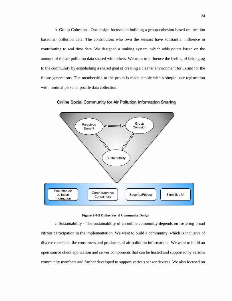
b. Group Cohesion - Our design focuses on building a group cohesion based on location
based air pollution data. The contributors who own the sensors have substantial influence in
contributing to real time data. We designed a ranking system, which adds points based on the
amount of the air pollution data shared with others. We want to influence the feeling of belonging
to the community by establishing a shared goal of creating a cleaner environment for us and for the
future generations. The membership to the group is made simple with a simple user registration
with minimal personal profile data collection.
Figure 2-0-5 Online Social Community Design
c. Sustainability - The sustainability of an online community depends on fostering broad
citizen participation in the implementation. We want to build a community, which is inclusive of
diverse members like consumers and producers of air pollution information. We want to build an
open source client application and server components that can be hosted and supported by various
community members and further developed to support various sensor devices. We also focused on

25
protecting privacy of user locations and restricting sharing of user profiles. Our design focuses on
members taking full ownership and responsibility of air pollution data they share.
2.5 Cloud Services Design
For the backend to our application, we needed a reliable server infrastructure to store,
process and push data to clients. We explored various options available for this purpose. Setting up
our own hosting server was one of the options, but it involves infrastructure and maintenance costs.
This was also not a very scalable option. Also a dedicated administrator would be required to
monitor and maintain the physical server.
Figure 2-0-6 Cloud Services Architecture
We would need to address connectivity, security and scalability in our infrastructure.
Another option was to use the readily available cloud infrastructure. Cloud web services provide
reliable, scalable infrastructure needed to deploy web solutions with least administration costs. We
want to design our remote web services to provide resizable compute capacity in the cloud so that
multiple virtualized instances can be provisioned to scale up or down capacity as the community
usage grows/shrinks. We have chosen Amazon Elastic Compute Cloud (EC2) to provide cloud-
hosting services. Amazon EC2 allows using web service interfaces to manage virtual operating
system instances, configure network security permissions and run multiple instances depending
upon the client request loads. We have adopted Representational State Transfer (REST) Web
services as they provide an easier-to-use, resource-oriented model to expose backend data services

26
for sharing air pollution data. Our implementation follows four basic design principles
Use of HTTP methods (GET/POST/PUT/DELETE) to establish one-to-one mapping
between create, read, update and delete operations.
Increase scalability by being stateless because stateless server-side components are less
complicated to design, write and distribute across load-balanced servers.
Simplified resource representations using directory structure-like URIs
Use JavaScript Object Notation (JSON) to transfer data as this reduces parsing overhead
and data mapping between data transfer objects
In order to simplify development of RESTful Web Services, we have used Java based Jersey Web
Services open source framework deployed on an open source Java Servlet container, Apache
tomcat. For storing sensor readings along with geographic location co-ordinates, we have used
PostGIS that is a spatial database extender for PostgreSQL object-relational database. PostGIS adds
support for geographic objects allowing location based SQL queries. The PostGIS implementation
makes use of lightweight geometries and indices, which are optimized to reduce disk and memory
usages, thereby improving query performance.
2.6 Pollution Sensing Inside Motor Vehicles
According to the report by the International Center for Technology Assessment (CTA),
levels of some air pollutants such as carbon monoxide (CO) are up to ten times higher inside
vehicles than at fixed monitoring stations [28]. The variations depended on the pollutant, the type
of road, the level of traffic and the type of vehicle being followed. Surprisingly, the study also finds,
due to the vehicle ventilation systems, the Particulate Particle (PM) pollution levels are 20-40%
lower inside the cars.
A highly polluting vehicle such as a heavy-duty diesel truck that is directly in front of a
motorist accounts for 50% pollution inside the car. Pollution inside the car was worse during
freeway rush hours and also while the car is driven in slow moving right lanes.

27
For the individual commuter, monitoring using a personal NODE device would facilitate
identifying dangerous pollution levels inside the car and take precautionary measures like rolling
down the windows during lesser traffic to increase air circulation.
Figure 2-0-7 Node Sensor Setup Inside Car
Studies conducted by EPA in the 1970s [29] shows that the pollutants in motor vehicles
find their way into their interiors. On many occasions, the pollutant levels inside cars are more than
those outside the vehicle. The pollution levels inside the cars are higher when traveling on heavily
congested roads or passing through busy intersections or while following diesel trucks or buses and
older cars. It is clear from the studies that pollution levels inside the cars are due to the exhaust
from other vehicles in the immediate vicinity. Based on a 1998 California Air Resources Boards
study [30], it is clear that especially very fine particle matter (PM) levels are higher inside car than
that of outside. Even though car's ventilation and air conditioning systems filter out larger particles,
passengers inside the car usually exposed very dangerous fine particles. As per studies by the
researchers from the Department of Environmental Health, Harvard School of Public Health [31],
the average in-car CO level is nearly 97% of the car exterior CO level average and was 3.9 times
the average for the ambient air CO level recorded by the remote CO monitoring sites. In the studies
CO levels inside the car ranged from 1 to 32 ppm, with an average of 11.3 ppm. CO levels

28
immediately exterior to the car range from 6 to 22 ppm with an average of 11.7 ppm. But the CO
readings from nearby fixed monitoring sites showed a range from 1.7 to 5.5 ppm with an average
of 2.9 ppm.
As per the model proposed by Flachsbart and Ah Yo (1989) [32] on commuter exposure to
CO, the total mass of CO within the vehicle interior is equal to the balance of the CO entered,
exited, emitted and reacted within the area volume inside the vehicle. The model predicts commuter
exposure to CO inside a car by exponentially diffusing CO concentrations just outside the car and
by exponentially decaying initial CO concentration that was already inside the car.
Average CO Exposure of the commuter = Observed CO Concentration on the roadway
+ (difference between CO concentration already present within the
vehicle and Observed CO Levels immediately outside the vehicle)
* (1-e tr/T) * (T/tr)
Where e = 2.71828 and T is the time constant in seconds and tr is the time the vehicle spends within
the roadway. The roadway CO concentration is dependent on traffic speeds, ambient temperature,
and types of vehicles present on the road, vehicle speed and number of vehicles present on the road.
Even though the actual commuter exposure to CO and other air pollutants is very dynamic and
varies depending on roadway CO concentration, our thesis focus is to share and communicate a
typical commuter exposure to CO concentrations to fellow commuters who would be travelling
under the same roadways and under nearly identical traffic situations.
2.7 Spatial Query Design
Spatial data is one that describes either a location or shape, for example, roads, house location,
rivers, municipalities, and lakes. Spatial data, in simpler terms, is represented as points, lines and
polygons. For example, roads can be represented as lines. Spatial data can be used to model
relationships between spatial objects like proximity, adjacency and containment. In conjunction
with other data, spatial data allows to model a complex spatial relationship. Spatial databases like

29
PostgreSQL with PostGIS extension allow us to treat spatial information as any other database
object. PostGIS allows us to use simple SQL expressions to determine spatial relationships like
distance, containment and perform spatial operations like intersection, area and union.
In our thesis, all of the sensor readings are collected along with longitude and latitude co-ordinates
from iPhone location services. The GPS co-ordinates are stored as a spatial data type of point.
In our model, the pollution data is collected when the user uses a sensor inside the car and
Figure 2-0-8 Spatial Design

30
travelling along the roadways. With the optimum time interval between successive sensor readings,
the GPS co-ordinates would closely map the shape of the roadways. The pollution information in
our design is conveyed to the user on a roadway map using Apple's MapKit interface. The pollution
data points are drawn over the map as polyline overlays. Because the map can be zoomed and
navigated around by the user, we use the maximum view port area co-ordinates and perform a
spatial intersect query to get all the GPS co-ordinates for which we have pollution data available
within a certain time frame (last two/four/six/eight hours) that lie within the rectangle area visible
on the map.
Air Quality Index Levels of Health Concern
Numerical Value
Meaning
Good 0 to 50 Air quality is considered satisfactory, and air pollution poses little or no risk
Moderate 51 to 100
Air quality is acceptable; however, for some pollutants there may be a moderate health concern for a very small number of people who are unusually sensitive to air pollution.
Unhealthy for Sensitive Groups
101 to 150 Members of sensitive groups may experience health effects. The general public is not likely to be affected.
Unhealthy 151 to 200 Everyone may begin to experience health effects; members of sensitive groups may experience more serious health effects.
Very Unhealthy 201 to 300 Health warnings of emergency conditions. The entire population is more likely to be affected.
Hazardous 301 to 500 Health alert: everyone may experience more serious health effects
Figure 2-0-9 EPA AQI Color coding
We developed a web service which would return a JSON array of pollution data along with
GPS co-ordinates given the max/min latitude and longitude values. The web service first creates
spatial envelope making use of area to be shown on the map by making use of ST_Envelope
function which returns a geometry object representing the bounding box defined by the corner
points. It then selects all of the pollution data points which intersects with the bounding box by
applying spatial intersects operator. This approach greatly reduces the amount of data exchange
and limits the data points to what can be reasonably viewed by the user using the map display. The
pollutant concentration levels are color coded as per EPA guidelines, as shown in Figure 2-0-9 [8]

31
for the air quality index calculated from the data points. It makes it easier for people to understand
quickly unhealthy air pollution levels they might experience along the roadways they are travelling.
For example, color green denotes the air pollution poses little or no risk while red denotes the air
pollution levels may be unhealthy for everyone.

32
Chapter 3
Implementation
This chapter describes the implementation details of the real-time mobile pollution sensing
online social community. In the opening section, the hardware components used in the
implementation are described. This is followed by the implementation details of the iPhone
application. It then describes the various modules used to implement server side components of the
online social community.
3.1 Hardware
Our key decision was to choose a commonly available gas sensor device, which is inexpensive,
easy to handle and use and one that also provides accurate real-time sensor readings. We have
chosen variable tech’s Node sensor OXA module as a preferred choice of gas monitoring device.
Very easy to attach OXA modules are available for Carbon Monoxide (CO), Nitric oxide (NO),
Nitrogen Oxide (NO2), Chlorine gas (Cl), Sulfur Dioxide (SO2) and Hydrogen Sulfide (H2S)[3].
The other end of the node device can be attached with Clima Module that can measure temperature
and humidity. Node device is especially very lightweight, inexpensive, easy to carry and ideal for
quick adaptation by the social community members. The node sensor can be used as it is inside the
car. For outside of car, we have built a prototype with easy to assemble components along with
Node sensor.
3.2 weBreathe iPhone Application

33
The primary goals of weBreathe iPhone application are ease of use and to provide timely,
accurate pollution information along the roadways. The first step in using the application is user
registration. The user profile consists of email address, password, node device id, pollutant sensor
type (CO/NO/NO2/H2S/CO2/CL2) and user preference to share sensor data using cellular data
plan or WIFI connection and option to select if user is interested in viewing pollution data for the
current user location or only for a certain zipcode. User sensor device registration is an optional
feature available. In the map display, user has an option to display last 8 hours of pollution data
with 2 hours intervals. weBreatheNavigationController class manages showing various
ViewControllers like LoginViewController, MapViewController and RegistrationViewController.
MainTabBarController presents tab bar with three options map, monitor and profile.
MonitorViewController class has the responsibility of interfacing with NodeDevice via
VTNodeManager Class and transmits pollution readings to the remote web service using RestClient
class. Depending upon the data sync option selected by the user and the available Internet
connectivity, the sensor readings are temporarily stored in the local SQLite database using the class
SensorReadingDAO.
Reachability class monitors change in Internet connectivity. NSTimer class is used to
schedule data synchronization activity at a predefined interval. Node device driver is used to
Figure 3-0-1 weBreathe iPhone Application User Interface Screens

34
interface to the Node device over Bluetooth connectivity. VTCoreLocationController class is
responsible for getting GPS location updates.
Figure 3-0-2 weBreathe Class Interaction Diagram
RestClient gets map display pollution data in JSON format from the remote web service and
interfaces with MapViewController to display map overlays of pollution levels.
3.3 weBreathe Web Services
To record sensor readings, we have developed a RESTful webservice called
Sensor_ReadingService, which takes in an array of JSON objects representing node sensor
readings. In order to simplify the development of RESTful webservice, we have used Jersey

35
RESTful Web Services framework. Jersey is an open source framework, which supports
developing java web services using JAX-RS apis. A JAX-RS resource is an annotated plain java
object that provides resource methods that are able to handle HTTP requests for URI paths that the
resource is bound to. In our case, the resource exposes a single resource method that is able to
handle HTTP POST requests, is bound to /Sensor_Readings URI path and can process an array of
Sensor_Reading objects represented in "application/json" media type.
Figure 3-0-3 weBreathe WebServices Class Interaction Diagram
TimeAdapter, DateAdapter and BlobAdapter classes are used to marshal and unmarshal time, date
and image objects in the JSON payload. Sensor_ReadingDAO class manages all of the PostgreSQL
database queries for saving sensor readings. Sensor_Reading class is the data transfer object (DTO)
representing a sensor pollution reading collected. UserManagerServlet supports all of the social
community functionalities like user registration, login, update user profile, map view based sensor
readings queries etc.

36

37
Chapter 4
Optimization
This chapter discusses various optimization techniques implemented in the mobile pollution
sensing online social community model. In the initial section, it lays down the goals of the
optimization process and explains what we intend to achieve by these optimization techniques.
Then, it briefly describes the details of the challenges and the solutions engineered to overcome
these challenges. Results of the optimization are then described to save network data usage,
smartphone battery power, amount of storage needed to store readings, map display efficiency and
timely sharing of pollution data with other online social community members. In the final section,
we explore a simple outlier elimination model to filter out temporal spikes in sensor readings.
4.1 Goals
In order to be an effective online social community for sharing pollution data, the model
should provide timely, accurate pollution information to its community members. Since the key
component in the model is the mobile application, it needs to be easy to use, provide a simpler user
interface to display pollution data along the roads. The client application must perform efficiently
on the iPhone platform by consuming least possible amount of battery power. There are two larger
groups of online social community users, consumers and producers of pollution data. Producers are
those members who carry the Node sensor devices inside their car and use the iPhone application
to measure the pollution levels as they travel and transmit data to the remote web services.
Consumers are those users who just use the iPhone application to know about the pollution levels
along the roadways they travel. For producers, the application needs to incur least amount of cost
for cellular data transfer. For consumers, the pollution map display should have high performance
and responsiveness with least amount of data transfer to reduce network overhead and battery
power consumption. Finally, the system should detect any temporary changes in sensor readings

38
and remove outlier values.
Our main goals for optimization can be listed as follows:
Efficient data transfer.
Reduced network data transfer cost.
Highly responsive map display with pollution overlay.
Reduce energy consumption of iPhone battery.
Removal of temporal spikes in sensor readings.
4.2 Data Transfer Optimization
Amount of data transferred between the iPhone device and the remote server impacts
battery power and data usage cost. Since most users of the weBreathe application might have
limited cellular data plan, our application is designed to use lower cost alternatives for network data
transfer. When the user is registering a Node device, user is given a choice to transfer sensor data
over 3G or only over Wi-Fi network. If the user has chosen Wi-Fi option, the data collected from
sensor is temporarily cached in the local SQLite database on the device, if there is no Wi-Fi network
available. The application receives notification from the iOS operating system if the network
interface changes to Wi-Fi. Once the device is connected to Wi-Fi, the application transfers sensor
readings in batches to reduce load on the server and as well as optimize battery energy usage. If the
user chooses to use 3G/4G cellular data plan, the gathered data is transferred in batches every 5
minutes. The 3G download and upload rates for the various Cellular providers is shown below [9].
Download(mbps) Upload(mbps)
ATT 2.62 0.85
Sprint 0.59 0.56
T-Mobile 3.384 1.44
Verizon 1.05 0.75
Average 1.911 0.9 Figure 4-0-1 3G Speeds (mbps) for Major US Cellular Providers

39
According to Apple specifications, iPhone 4S has a Lithium-Ion battery with a capacity of 1420
mA-h. At 3.7 volts, it translates into 5.254 Watt-hours and could support Internet activity for up to
six hours. IPhone 4S consumes 0.875 W (5.254/6) per hour for Internet activity. On an average of
1.9 mbps download rate, iPhone 4S could download 858 MB data per hour and at 0.9 mbps upload
rate, it could upload 405 MB data per hour. weBreathe iOS application uses 300 bytes of data per
sensor reading and could upload 1350000 readings per hour (405 MB/300 bytes). Our design
balances to reduce the overhead associated with establishing a TCP socket connection and tearing
it down, amount of data that can be transmitted in a single upload, time it takes to upload and
processing overhead associated with large number of JSON array objects at the web services layer.
If we assemble an array of 25 such sensor readings as an array of JSON objects and upload it during
a single HTTP request, it takes 7.5 KB of data transferred in 66 milliseconds. We arrived at twenty
five array size based on the calculations involving maximum number of readings possible if the
user
travels at maximum of 65-75 mph and if we collect readings for every 0.25-mile interval. The
iPhone system turns off Wi-Fi and cell radios when it detects a lack of activity. It is more energy
efficient to transmit data in a shorter amount of time than continuously over longer periods of time.
Figure 4-0-2 weBreathe Energy Usage Analysis

40
Based on energy analysis using XCode instrumentation, there is direct correlation between data
upload and energy usage. It is clear that smaller increases in energy usage are associated with
smaller burst of data upload. Further data transfer optimization can be achieved by increasing time
interval between data uploads and increasing batch size. But this would degrade the real time
pollution data availability to other community members.
4.3 Data Transfer Cost Optimization
On an average, 3G cellular data plan cost $10 per 1GB of data transfer. If an average
weBreathe application user monitors pollution data for eight hours per day for thirty days and if
7.5 K data is transmitted at the rate of every 5 minutes, the user would normally use 21.6 MB of
cellular data plan, which translates to 21.6 cents of expense per month. We have implemented gzip
algorithm to compress the sensor readings before it gets transmitted to the server. Tomcat server
and Jersey Framework are custom configured to enable gzip compression support using jersey
plugins. weBreathe iPhone application connects to tomcat server and notifies server that it supports
gzip “Content-Encoding:gzip” and sends compressed data using gzip algorithm. Tomcat server
acknowledges gzip support and decompresses input data using gzip.
GZIP compression works by finding similar strings within the JSON payload and replacing
those strings temporarily to make overall payload smaller. This type of compression is well suited
Figure 4-0-3 weBreathe uses gzip Compression to Reduce Data Plan Cost

41
for the JSON payload because the key values are often repeated in a collection of sensor readings.
GZIP employs deflate data compression algorithm that uses a combination of the LZ77 algorithm
and Huffman coding. We have found with maximum gzip compression ratio used, the data payload
size is reduced by 90%. The 7.5k JSON payload mentioned above, is reduced to 768 bytes, thereby
reducing the cost of data plan usage by 90%, hence reducing the cost to almost 2 cents per month.
GZIP compression also reduces the battery energy consumption considerably because it
transmits reduced amount of data per sync up cycle.
4.4 Pollution Map Display Optimization
The user interface to convey air pollution information along the roadways is the map
display at the street level. We have used the MKMapView object to display the pollution data over
the map view. User can zoom in or zoom out and move around the map display. The pollution
information is dynamically retrieved from the remote web service. Each pollution record contains
GPS coordinates (longitude, latitude) and pollutant AQI index. We have used MKPolyline object
to connect these pollution coordinates as polyline with color-coding based on the AQI value.
MKPolyline overlays over the roadways, thereby providing a graphical display of pollution levels
to the user. The optimization techniques employed involves the following
1. Instead of displaying every point, combine nearby points based on pollution level
2. Use background threads to load data and display in batches
3. Display only those points that are visible on the map display
4. Cache overlays and reuse to reduce memory footprint.
We have evaluated Douglas-Peucker algorithm [45] to combine nearby points. The
algorithm starts an edge with first and last points of the polyline; the remaining points are tested
for the closeness to the edge. If there are points further away than specified tolerance level from
the edge, then the point furthest from it is added to the polyline. This creates a new approximated
polyline. Using recursion, this process continues for each point of the polyline until all points of
the original polyline are processed.

42
In order to limit the number of points that can be displayed over the map, we have used
spatial query with the PostGIS function ST_Intersect to retrieve points that are contained within
the map max and min co-ordinates. It greatly improved the map display performance and reduced
the amount of data that is retrieved from the webservice, thereby further optimizing energy
efficiency of the application. MKOverlay objects are cached in memory and reused, thereby
reducing the amount of memory needed to display pollution data as the user scrolls around the map
display.
We also evaluated various GPS location update optimization techniques such as turning
off location manager services when the user is not moving and reactivating location manager
updates based on local accelerator movements.
4.5 Outlier Detection
Because of the initial settling time required for the various electrochemical gas sensors,
they might show abnormal AQI values. It is important to detect such outlaying sensor readings.
Usually such outliers are considered noise and thus need to be discarded in order to obtain a reliable
pollution reading. One of the simplest outlier detection algorithms is Chauvenet's criterion [46],
which uses the mean and standard deviation calculated from the sample to determine a "normal"
range for values. Any value outside of this range is deemed an outlier.
The problem with Chauvenet's criterion is it assumes normal distribution of data values.
Unfortunately, in our case, the pollution data varies by location and various environmental factors.
One reasonable assumption we could make is pollution data follows a normal distribution in a
specific geo location area, for example, area with in a zip code. We have adapted Chauvenet's
criterion because of its simplicity but we limited our outlier removal based on the geo location
points contained within the geometrical area of a zip code. For this we have used geo spatial
database containing all zip codes in US and used ST_Contains PostGIS spatial query to retrieve all
of the sensor readings obtained within an area covered by a zip code and applied Chauvenet's

43
criterion to remove any outlier data. The outlier processor is implemented as part of server process
that wakes up every three hundred seconds and runs in the background to mark any outliers. When
data is retrieved from the app for diplay, the outliers are not pushed.
We believe zip code pollution data normalization is a reasonable assumption to remove
any outliers and Chauvent’s criterion proves to be an efficient algorithm to remove temporal spikes
in sensor readings.
4.6 Speed Based Sensor Reading
Speed based data gathering involves enabling data collection only when the user is moving
above a predetermined speed. In the situation where the iPhone automatically pairs with Node to
start collecting data, we would want to avoid scenarios where the Node is static but the application
repeatedly collects pollution data for the same location. Tracking the speed will determine the user
in motion on the street and thus enforce data collection when device is in a vehicle travelling on
the road. iOS Location Services (GPS) provide Speed parameter along with latitude and longitude
values. Based on this speed value, we dynamically calculate the number of readings to be collected
per time unit based on the assumption that we need pollution level readings at constant distances
(for example, one reading per 0.25 mile). If the user is travelling at sixty miles of hour, we need to
sample sensor readings at fifteen seconds interval so that we gather one pollution level reading
every 0.25-mile.

44
Chapter 5
Evaluation
The purpose of this chapter is to discuss the evaluation of various components of mobile
pollution sensing social model and to discuss the results from comparing pollution data from the
mobile model with NJ DEP (Dept. of Environmental Protection) stationary central monitors. It
starts with the goals of the evaluation approach. Then, it describes the data flow samples from
various components, starting from node sensor to the iPhone application, then to the back end server
and then back to an iPhone for consumption. It also illustrates calibration techniques used to arrive
at baselines for CO sensors at EPA laboratory. Then, it describes the details of the field study from
data captured using the mobile pollution-sensing model at and around NJ DEP stationary monitor
at Newark, NJ. The results of the evaluation are then analyzed for accuracy and timeliness. In the
final section, we explore the advantages of using such dynamic mobile sensing model and how it
could augment the existing DEP stationary sensors.
5.1 Goals
For a mobile-based pollution model to be effective, the Node gas sensor should be sensitive
enough to accurately detect varying pollutant levels in the atmosphere. The gas sensor should also
have shorter settling times and they must be quick to detect pollutant gas levels as early as possible
so that commuter is alerted in a timely fashion. The pollution data should also be available in real
time to other users who are travelling on the same road or location. The application should perform
efficiently to save battery power on the mobile device, reduce storage requirements on the server
and optimize the amount data exchanged over the network. It should also be scalable to support
thousands/millions of social community users. Our evaluation goal is to try to address these
objectives to validate the feasibility and practicality of mobile sensing model.
The main goals of evaluation are:

45
1. Validate real time responsiveness of data exchange and sharing among other users.
2. Provide effective use of resources such as battery power, network bandwidth, storage and
processing time.
3. Assure effectiveness of outlier detection.
4. Ensure accuracy and precision of Node sensors by calibration against standard gases
5. Field study of NJ DEP stationary central gas monitor vs. mobile pollution sensing monitors.
5.2 Real-time Responsiveness
In our model, exchanging real time pollution information with other users is vital for its operational
success. Efficient data exchange and optimized network and data usage reduces the time lag
between data generation and data consumption. The model has two modes of operation, monitoring
and pollution map view modes.
Pollution Map View mode has the following set of operations
1. User Registration (One time)
2. Login
3. Pollution Map view
Monitoring mode has the following set of operations
1. User Registration (One time)
2. Device Registration (One time)
3. Baseline Calibration of Node Sensor (One time)
4. Login
5. Pollution Monitoring
We measured the performance of each operation based on the system clock time on the
mobile device. The clock time includes CPU time, network round trip time and server processing
time. Baseline calibration is performed using Node application named NodeOXA and it would
take 5 mins an average per device for one time calibration of the baseline. Upon calibration, the

46
baseline value is stored in the ROM memory of the Node device itself and can be queried by Node
API. Based on the device logs, the average time for each of the operation is shown on the graph
below
Figure 5-0-1 Execution Time for Operations
The execution time is dependent on various factors like network speed, load on the server and
number of the concurrent users etc. We estimate each operation to take less than 1 sec under normal
operating conditions and real time sharing of pollution data could happen within couple of seconds
of uploading the data to other community users.
5.3 Outlier Detection
Outliers are deviant sensor readings away from the normal level of CO PPM expected in a
certain geo location. Outliers could occur due to various reasons. In our prototype, we observed,
the outlier readings are mainly due to initial settling time required for the gas sensor. When the
monitoring is turned on in the node sensor, it starts with very high PPM readings and within a
couple of minutes, it settles down and starts giving normal readings. We also observed it happens
every time monitoring is turned off and turned on again. The other occasions we see sudden spikes
in readings are when the sensor exposed to sudden high levels of CO, for example a heavy truck
passing by and cold start of motor vehicles. The purpose of our study is not only to identify outliers
0 200 400 600 800
User Registration
Device Registration
Readings upload
Mapview
Login
Execution Time (millisecs)
Execution Time (millisecs)

47
and also arrive at an approach to manage them. We want to flag outliers due to sensor's initial
settling at the client level and other types of outliers at the centralized back end server. Based on
heuristic, we arrived at an initial settling count of readings that can be safely ignored when the node
sensor is turned on for monitoring. We have designed a background process that periodically wakes
up (every 5 minutes) and analyzes the latest readings recorded per geo location. In our case, we
have chosen to use the geo location area covered by a US zip code. We have pre-populated all of
the zip codes and its spatial dimensions (shape files) from census.gov website into our POSTGIS
database table.
We have used Chauvenet’s criteria as the basis for outlier detection.
Algorithm for zip code based spatial query for outlier detection:
1. Get all of readings recorded since the last run
2. Get a list of zip codes by applying spatial query ST_Contains to check if the longitude and
latitude of the reading location falls within the zip code spatial dimensions.
3. Calculate the average and standard deviation of the all of the readings for each of the zip
code.
4. Calculate complementary error function erfc [ reading – average/std dev].
5. If the erfc value is less than 0.5 (1.96 std dev), flag the reading as outlier in the database.
Figure 5-0-2 Outlier Detection

48
Any value marked as outlier is not displayed on the pollution map but the reading is retained in the
database for further analysis.
For example for the zip code of 07095, the outliers are marked in the outliers region as
shown.
As shown above in the figure 5-0-2, the outliers are illustrated with a color red. When the node
device is turned on, the initial settling values are identified as outliers and not displayed on the
pollution map. The intermitted spikes in values are correlated with turning on and off of the node
device.
When outlier batch job is run, it picks up all of the new readings since its last run and applies
the outlier detection algorithm for each of the zip code region that readings geo co-ordinates fall
under. For example, the reading id 365204 with a ppm value of 13.879 is marked as an outlier for
the zip code 07095 because it is more than 1.96 standard deviations of the other readings for the
zip code location. The server log indicating outlier detected is included in Appendix A.
5.4 Data Flow Illustration
weBreathe iPhone application uses iOS Bluetooth framework to connect to the node sensor.
Once it is connected, the user turns on monitoring by selecting the monitor button. Once the monitor
button is selected, the application requests Node sensor to stream CO pollution readings at a
predefined time interval (in units of 10 milliseconds). For example, weBreathe application uses 100
units as sense interval which means it requests updates every second. weBreathe application uses
node API shared library to interface with node sensor. All of the API communication is based on
call back mechanism. For example, when the Node module is ready for communication, it calls
nodeDeviceIsReadyForCommunication method. Our iPhone application initializes Node device,
queries for CO baseline reading, queries for all of the sensor modules on the device and once it
receives callback, it refreshes the user interface with type of gas sensor modules and CLIMA
module details for getting humidity and temperature details.

49
weBreathe application collects a predefined set of readings and uploads the readings as a gzip
compressed JSON array to the backend server as a HTTP post. The phone log in Appendix B
illustrates sensor data capture and transmission.
Due to the compression technique, we could see the original payload size of 5576 bytes is
reduced to 594 bytes which around 90% savings in the data transmission. For example, in the
picture shown, the storing of reading took four hundred ninety five milliseconds to execute. Our
backend server (IP Address 165.230.44.85) runs a tomcat server at port 8080. Our server clock is
skewed by -751 seconds than the mobile phone. The J2EE application Sensor_ReadingsService
uses UserManagerServlet to record readings. The Server access log in Appendix C shows the client
IP address, type of request, result of the request and how many milliseconds it took to complete the
request.
Figure 5-0-3 Map View and Response Data Illustration
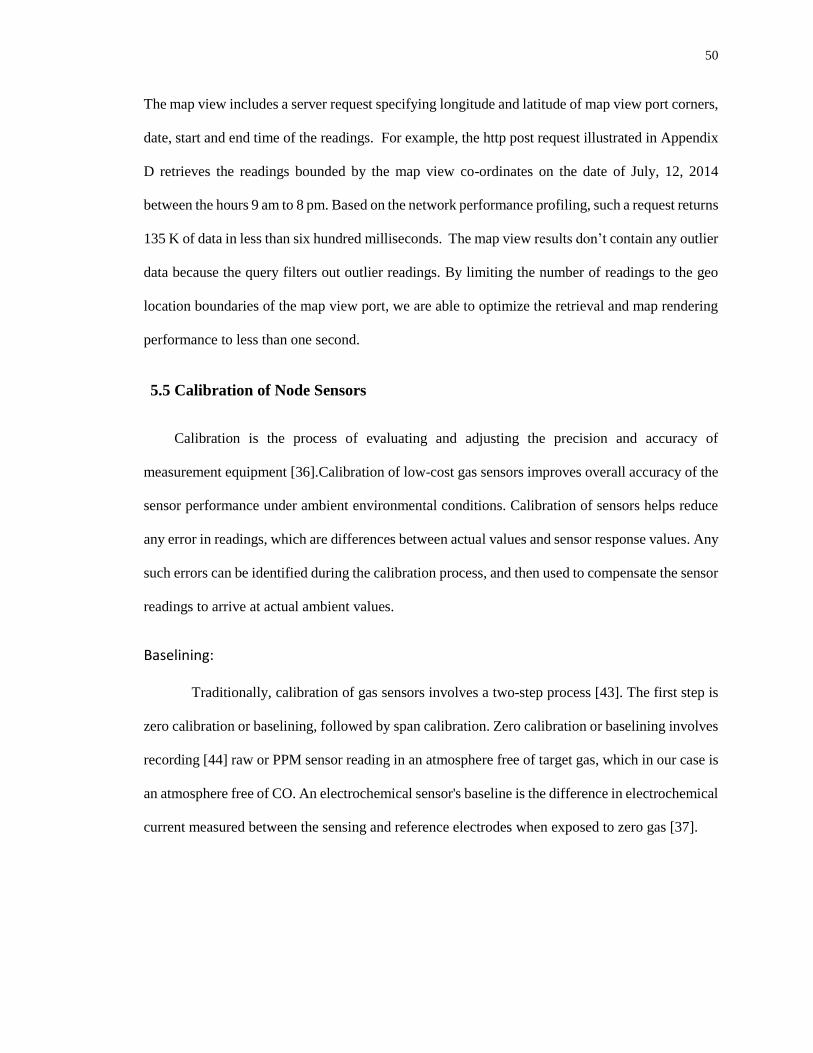
50
The map view includes a server request specifying longitude and latitude of map view port corners,
date, start and end time of the readings. For example, the http post request illustrated in Appendix
D retrieves the readings bounded by the map view co-ordinates on the date of July, 12, 2014
between the hours 9 am to 8 pm. Based on the network performance profiling, such a request returns
135 K of data in less than six hundred milliseconds. The map view results don’t contain any outlier
data because the query filters out outlier readings. By limiting the number of readings to the geo
location boundaries of the map view port, we are able to optimize the retrieval and map rendering
performance to less than one second.
5.5 Calibration of Node Sensors
Calibration is the process of evaluating and adjusting the precision and accuracy of
measurement equipment [36].Calibration of low-cost gas sensors improves overall accuracy of the
sensor performance under ambient environmental conditions. Calibration of sensors helps reduce
any error in readings, which are differences between actual values and sensor response values. Any
such errors can be identified during the calibration process, and then used to compensate the sensor
readings to arrive at actual ambient values.
Baselining:
Traditionally, calibration of gas sensors involves a two-step process [43]. The first step is
zero calibration or baselining, followed by span calibration. Zero calibration or baselining involves
recording [44] raw or PPM sensor reading in an atmosphere free of target gas, which in our case is
an atmosphere free of CO. An electrochemical sensor's baseline is the difference in electrochemical
current measured between the sensing and reference electrodes when exposed to zero gas [37].

51
Figure 5-0-4 Lab Setup for Baselining of Nodes
In Rutgers Environmental Science lab, a sealed container with valves, to ensure constant
pressure within the enclosure, was used for the experiment. A CO free environment was created
within the container by introducing argon gas for approximately fifteen minutes. This simulated a
0 ppm of CO environment. The raw values measured by the CO sensor in this simulated 0 ppm
environment were noted, using the Node+OXA application, as the baseline, as shown in Fig 5-0-5.
This same experiment was performed across six available Node sensors and was repeated seven
times for each of the Nodes. Node sensor stores the baseline raw value in its memory so that it can
be retrieved using Node API interface for PPM calculations in the mobile app. We also derived
method detection limit, as shown in Appendix E, to ensure that the readings were not due to sensor
noise and to establish the lowest CO concentration that can be measured using Node sensors.

52
Figure 5-0-5 N+Oxa app for Baselining
Calibration:
The next step in calibration is span calibration, in which premixed calibrated gases are
exposed to sensor and statistical methods in calibration are applied. In our study, six baselined
Node sensors were used for the span calibration. We conducted the calibration experiments in EPA
(Environment Protection Agency) lab in Edison, NJ. The baselined Nodes ensured that the sensors
were capturing the most precise CO readings in ppm. Another larger enclosure to contain the Node
sensors was used for this experiment. Different concentrations of CO gas were introduced into this
chamber through a multigas calibrator- Environics Series 6100 Computerized Multi-Gas
Calibration System and allowed to stand for 20 minutes. The calibration set up is shown in Fig 5-
0-6 and Fig 5-0-7. The values captured from weBreathe application for CO level in ppm,
temperature and humidity were recorded and regression analysis was performed.[39] (As shown
in fig 5-0-8).
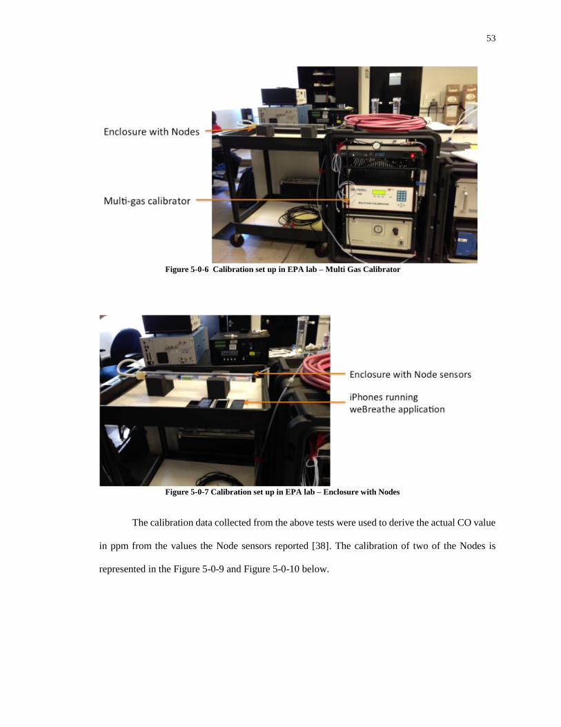
53
Figure 5-0-6 Calibration set up in EPA lab – Multi Gas Calibrator
Figure 5-0-7 Calibration set up in EPA lab – Enclosure with Nodes
The calibration data collected from the above tests were used to derive the actual CO value
in ppm from the values the Node sensors reported [38]. The calibration of two of the Nodes is
represented in the Figure 5-0-9 and Figure 5-0-10 below.

54
Figure 5-0-8 Regression Analysis of Calibration Data
Figure 5-0-9 Linear regression Node 472A55E8BD60

55
Figure 5-0-10 Linear regression Node C4CFF5431C24
Measurements gathered from Node devices were corrected by the inverse of the calibration
curve. From plotting the data and applying linear regression statistics, the calibration equation (i.e.,
the gradient and the intercept) is used to estimate the concentration of CO in field studies [40].
Applying the calibration curve on values collected from Node sensor eliminates instrument
bias provides accurate values when the sensor is deployed in the field. The actual values of CO in
ppm derived for two of the Node sensors were as follows, from inversing the calibration graph:
NODE-472A55E8BD60 : actual_value = (Node reading - 0.3472)/1.0774
NODE-C4CFF5431C24 : actual_value = (Node reading + 0.2674)/1.1596
5.6 Study of Mobile Sensing Model Data in Comparison to Stationary Central
Monitor
The calibrated Nodes were used for a field study conducted to compare our mobile pollution
sensing model with existing central air pollution monitors. The objective of our field study is to

56
demonstrate spatial granularity of pollution data along the roadways. As part of this analysis, we
conducted a field study of pollution data collection using Node sensors inside a car, windows
closed, as a typical commuter would do, driving along the road ways. We compared our results to
pollution levels reported by a certified stationary monitor.
The Department of Environmental Protection in New Jersey (NJ DEP) has various central
monitoring stations located across the state of NJ to monitor and predict air quality. These central
monitoring stations have sensors for monitoring pollutants such as CO, O3, SO2, NO2 and PM
2.5[41]. The reports from these stations are available for public consumption via email, website or
mobile application.
For our study, we chose the stationary monitoring station located at Newark Firehouse at
Newark, NJ since it has a CO monitor that we could compare against and the location was easily
accessible.
The primary goals of the study are
1. Compare central monitoring station data with data gathered from mobile pollution sensing
social model.
2. Evaluate the precision and accuracy of data collected from mobile pollution sensing social
model, using statistical analysis
3. Analyze spatial granularity of data at various distances at and around the stationary
monitoring station.
Our study procedure involves collection of data at various roadways near the stationary
monitor, apply calibration error correction to derive true CO concentration and analyze the data
using statistical tools.
The first step in our study was to visit the NJ DEP Newark Firehouse monitoring station and collect
readings by:
- Standing right next to the NJ DEP monitoring station with 3 Nodes and 3 iPhones running

57
Figure 5-0-11 NJ DEP Newark Firehouse Monitoring Station
weBreathe application
- Driving along the streets adjacent to the NJ DEP monitoring stations with two Nodes placed
near vent inside car using weBreathe application on two iPhones
- Driving along streets that were approximately 0.5 miles away from the NJ DEP monitoring
station with two Nodes placed near vent inside car using weBreathe application on two iPhones
- Driving along streets that were approximately 2 miles away from the NJ DEP monitoring
stations with two Nodes placed near the vent inside car using weBreathe application on two
iPhones.
The next steps for evaluation of data collected were (represented in Fig 5-0-13, Fig 5-0-14,
Fig 5-0-15 and Fig 5-0-16 below):
- Applying calibration function on data collected from Nodes.

58
- Splitting data collected into segments of 60 second intervals so there were greater than thirty
Figure 5-0-12 weBreathe iOS app Displaying Pollution Levels Around NJ DEP Station
samples in each segment across three Nodes(if sample size is large (n>=30), then the sample
standard deviations can be used to estimate the population standard deviation)[42]. This enables us
to study the distribution of pollution data among monitors and distribution across distance.
- Calculating the mean CO level for each segment of data
- Calculating standard deviation and margin of error for each set of data, averaged over a time
period of 60 seconds and over the same distance from central monitor
- Plotting the NJ DEP monitor CO level to compare against the pollution data captured from
mobile pollution sensing model

59
Figure 5-0-13 Mobile Pollution Sensing Data at NJ DEP Monitoring Station
Figure 5-0-14 Mobile Pollution Sensing Data at Immediate Vicinity of NJ DEP Monitoring Station

60
Figure 5-0-15 Mobile Pollution Sensing Data at 0.5 mile Distance from NJ DEP Monitoring Station
Figure 5-0-16 Mobile Pollution Sensing Data at 2 mile Distance from NJ DEP Monitoring Station
Conclusions from field study:
- Calibration against standard gases and linear regression analysis applied to data
demonstrates accuracy of data collected
- Data collected from mobile pollution sensing model demonstrates spatial granularity of air
pollution along roadways

61
Figure 5-0-17 Map summarizing spatial granularity of pollution data
- Mobile pollution sensing model effectively captures the spatial granularity of pollution
data and provides timely representation of air pollution to commuters.

62
Chapter 6
Future Directions
In this chapter, we present several areas of further research that can be explored in order to
expand the work proposed by this thesis. We first discuss how we need to device appropriate sensor
maintenance techniques to ensure the quality of data. We then discuss how we can apply some
mechanisms to address privacy concerns of users sharing pollution data. This is followed by
discussion of the various enhancements and optimizations that could be incorporated into the iOS
application and backend server to personalize usage of the app as well as adding additional features
to improve the efficiency and effectiveness of the data provided to users. Subsequently, we present
how this model can be effectively used as the means to conduct various studies related to air
pollution. We then discuss how the mobile pollution sensing model could lay a foundation for
cleaner route guidance as well as eventually be incorporated in the larger scope of vehicular
networks.
6.1 Sensor Maintenance
The calibration techniques mentioned in section 5.5 will ensure the quality of data
measured using the mobile pollution-sensing model. But subsequent periodic calibrations are
required to ensure quality of measured data using the mobile platform[48] . We need to arrive at
techniques to enable members of the mobile pollution sensing social community to periodically
calibrate their devices against a reference-calibrated device. Sensor decay, where the sensor
degrades with time, is another issue to be addressed. We could use techniques where the mobile
app will runs regular checks to ensure that the sensor is performing accurately and give alerts when
recalibration of sensor or replacement of sensor is required.
6.2 User Privacy
Since our model involves sharing the air quality information along the streets on a map, we

63
need to address any privacy concerns of users participating in our model. This would be addressed
as the amount of data coverage is improved by high level of participation from the members since
it will be difficult to track the routes of any particular participant collecting pollution data. Applying
techniques such as removing the first and the last mile in the readings gathered will ensure that
even if there are few users collecting pollution data in a certain location, it will not be feasible to
see the precise locations that the user travelled.
6.3 iOS Application and Backend Improvements
Cumulative exposure alert: The application could be improved by the calculation of
cumulative pollutant exposure of user in a day. As per the EPA standard, 36 FR 8186[10] CO
exposure standards were set at 9 parts per million (ppm), as an eight hour average, and 35 ppm, as
a one hour average, neither to be exceeded more than once per year. The average driver is not aware
of the extent of cumulative exposure to air pollutants. Especially, for a user that spends a lot of time
travelling on the roads, this would prove to be very valuable information. The application could
calculate the cumulative exposure of the user and alert users.
Social networks integration: Social network integration could be added to the iPhone
application enabling the user to share pollution data or pollution map snapshot posting over
Facebook or Twitter like applications. This would not only motivate the users to collect more data,
but also encourage friends and followers on these social networking sites to connect, collaborate
and share air quality data.
Multiple device support: Currently our social model and iOS application supports the use
of Node sensors. This can be easily expanded to enable usage of multiple gas sensors from different
vendors. The app could be customized based on the sensor device that it is paired with.
Redundant data elimination: On the backend server, we could implement further
optimization by tracking multiple users collecting data on the same road segment within the same
time frame and enable push notifications to the devices from the server to stop collecting duplicate
data. When it is detected that the user has moved to a new road segment, the monitoring could be

64
restarted. These optimizations would further reduce redundant data usage and also conserve energy.
Multiple reading: A different approach that could be taken to handle multiple data points
from the same road segment would be to utilize the multiple readings to arrive at the most accurate
pollution level for that region. Removal of outliers from readings for same region would verify the
accuracy of the pollution data.
Archive historic data: Another possible optimization on the server database would be to
archive any stale data. Say all the readings that are more than a day old could be compressed and
archived. Also, an eight hour average of pollutant level could be extracted from historic data and
used to demonstrate pollution trends for various road segments.
Incorporate EPA data: The data presenting in the application is the pollution data collected
from participating users of the social community alone. Incorporating data collected from various
other air pollution monitoring systems can broaden the coverage. The EPA, for instance, maintains
a repository of ambient air quality data in the Air Quality System (AQS). We could include a
backend service to regularly pull the AQS data incorporate it with the data collected from the social
community. The weBreathe app can then display the data from AQS for regions where no
participating users have collected air quality data.
6.4 Data Studies
Using the mobile pollution-sensing model presented in this thesis, air pollution data could
be collected for various studies. How air quality is affected by meteorological factors such as wind
speed, temperature, humidity, pressure and climatic factors could help in creating prediction models
for air pollution. Further studies could be conducted to find correlation between traffic patterns,
vehicle speed and air pollution. Studies could be conducted to model the pollution propagation
from point of emission and distribution to nearby locations. An interesting study could be
conducted to compare the pollution levels inside the car with the ambient pollution level just outside
the car.
Machine learning techniques could be applied to predict future pollution levels based on

65
historic data collected using the mobile pollution-sensing model. Such predictive models can be
used to make future city and roadway grid planning decisions. A user study can be conducted to
analyze how the air quality information provided by our model impacts the behavior of users. It
would be interesting to note how many commuters actually take alternate clean routes at the cost
of additional travel times.
6.5 Green Routing
The launch of solutions such as Car-Play by Apple is a clear indicator of how connected
vehicles would be in the near future. The addition of air pollutant sensors incorporated within motor
vehicles does not seem a distant possibility. The vehicles in-built sensor technology combined with
solutions such as Car-Play and ubiquitous Internet connectivity would enable us to provide highly
accurate, real-time air pollution data with extensive coverage. We would be able to easily assimilate
the air quality data over traffic maps to enable route guidance based on cleaner routes. An
interesting study could be conducted on human behavior to analyze how often commuters actually
choose to take a cleaner route by compromising travel time. Another approach to available pollution
data is that altruistic citizens might even avoid heavily polluted streets so they can avoid causing
higher pollution.

66
Chapter 7
Conclusion
In this thesis, we introduced the design and implementation of a mobile pollution sensing
social community to enable the gathering and sharing of air quality data. We proposed a model that
overcomes the shortcomings of current pollution monitoring methodologies. The design of the
model involved selection of an appropriate device to measure pollutant levels and interfacing it
with a smart phone application. By connecting a cloud service to a mobile application, we presented
the feasibility of a real time pollution collection and sharing social model. By applying various
optimization techniques at the application and web service level, we were able to make the model
highly efficient and cost effective.
The key conclusions of this thesis are:
Real time pollution information sharing is practical with adoption of mobile-cloud
integration
Highly efficient location data management can be achieved with the aid of spatial data
model
Optimized use of mobile battery energy is feasible with data compression and efficient
location based data exchange
We could use the model to collect data for both internal and external to motor vehicles
Simple online social community model can be realized with two groups of members,
consumers and producers.
Mobile pollution sensing model captures spatial granularity of pollution data.
In this current day and age, smartphones are an integral part of our lives and put immense
computing power and connectivity in the hands of users, thereby opening up a world of
opportunities. Leveraging this technology to connect citizens with the common interest of air

67
pollution awareness provides a highly practical solution to gather fine-grained air quality data.
The increased adoption rate of this social community would translate into making the pollution
data highly accurate and precise.
The applications of the data collected from our model is innumerous, starting from users
utilizing it to guide their travels every day, to sensitive commuters avoiding more polluted
routes. On a larger scale, the data could prove valuable in making informed decisions even for
establishing schools or residential communities. This model opens the doors for exploring
innovative opportunities to create a cleaner world.

68
Appendix A
Server Logs Indicating Outlier Detection

69
Appendix B
Phone Logs Illustrating Sensor Data Capture and
Transmission
2014-07-01-09:19:10 Current Sense interval = 100.000000 2014-07-01-09:19:10 Current Batch size = 10
2014-07-01-09:19:10 Internet connection 3G available
2014-07-01-09:19:10 Internet connection 3G available 2014-07-01-09:19:10 Internet connection not available
2014-07-01-09:19:10 Internet connection 3G available
2014-07-01-09:19:10 notifiedThatNodeDeviceIsReady 2014-07-01-09:19:12 nodeDeviceIsReadyForCommunication
2014-07-01-09:19:13 nodeDeviceDidUpdateModuleSubTypes called
2014-07-01-09:19:13 OXA baseline = 0.199435 2014-07-01-09:19:13 nodeDeviceDidUpdateModuleSubTypes called
2014-07-01-09:19:13 OXA baseline = 0.199435
2014-07-01-09:19:14 Before Monitor Battery level 95.00 2014-07-01-09:19:14 Speed on location update= 1.88
2014-07-01-09:20:37 Raw reading = 0.199976
2014-07-01-09:20:37 ppm = 1.723120
2014-07-01-09:20:38 Raw reading = 0.199806
2014-07-01-09:20:38 ppm = 1.622736
2014-07-01-09:20:39 Raw reading = 0.200707
2014-07-01-09:20:39 ppm = 1.707382
2014-07-01-09:20:40 Raw reading = 0.200215
2014-07-01-09:20:40 ppm = 1.687971
2014-07-01-09:20:41 Raw reading = 0.200369
2014-07-01-09:20:41 ppm = 1.700468
2014-07-01-09:20:42 Raw reading = 0.200198 2014-07-01-09:20:42 ppm = 1.678569
2014-07-01-09:20:43 Raw reading = 0.200218 2014-07-01-09:20:43 ppm = 1.662803
2014-07-01-09:20:44 Raw reading = 0.199210 2014-07-01-09:20:44 ppm = 1.452895
2014-07-01-09:20:45 Raw reading = 0.199921 2014-07-01-09:20:45 ppm = 1.401922
2014-07-01-09:20:46 Raw reading = 0.200202 2014-07-01-09:20:46 ppm = 1.410717
2014-07-01-09:20:46 Original Payload = [{"environment_Light":0,"reading_PPM":1.72312,"reading_interior_exterior_flag":"E","reading_travelling_vehicle_type":
"car","device_ID":"5DD8F0C0-49BD-67AA-B895-BBDAA916CE2D","gps_Longitude":-
74.360055,"reading_ID":"0","environment_Temperature":0,"gps_Latitude":40.512153,"gas_Type":"CO","environment_Atmospheric_Pressure":0,"device_Name":"NODE-
472A55E8BD60","reading_travelling_flag":"y","username":"[email protected]","reading_Raw":0.200323,"reading_Time":"0
9:20:37","aqi":19.580906,"environment_humidity":0,"gps_Speed":1.88,"reading_Date":"2014-07-01 09:20:37"},{"environment_Light":0,"reading_PPM":1.622736,"reading_interior_exterior_flag":"E","reading_travelling_ve
hicle_type":"car","device_ID":"5DD8F0C0-49BD-67AA-B895-BBDAA916CE2D","gps_Longitude":-
74.360055,"reading_ID":"0","environment_Temperature":0,"gps_Latitude":40.512153,"gas_Type":"CO","environment_Atmospheric_Pressure":0,"device_Name":"NODE-
472A55E8BD60","reading_travelling_flag":"y","username":"[email protected]","reading_Raw":0.200271,"reading_Time":"0
9:20:38","aqi":18.440187,"environment_humidity":0,"gps_Speed":1.88,"reading_Date":"2014-07-01 09:20:38"},{"environment_Light":0,"reading_PPM":1.707382,"reading_interior_exterior_flag":"E","reading_travelling_ve
hicle_type":"car","device_ID":"5DD8F0C0-49BD-67AA-B895-BBDAA916CE2D","gps_Longitude":-
74.360055,"reading_ID":"0","environment_Temperature":0,"gps_Latitude":40.512153,"gas_Type":"CO","environment_At
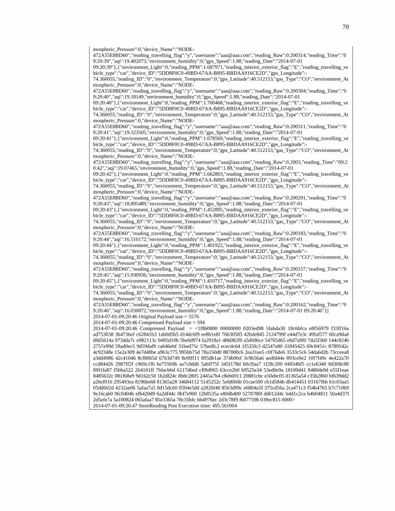
70
mospheric_Pressure":0,"device_Name":"NODE-
472A55E8BD60","reading_travelling_flag":"y","username":"[email protected]","reading_Raw":0.200314,"reading_Time":"09:20:39","aqi":19.402073,"environment_humidity":0,"gps_Speed":1.88,"reading_Date":"2014-07-01
09:20:39"},{"environment_Light":0,"reading_PPM":1.687971,"reading_interior_exterior_flag":"E","reading_travelling_ve
hicle_type":"car","device_ID":"5DD8F0C0-49BD-67AA-B895-BBDAA916CE2D","gps_Longitude":-74.360055,"reading_ID":"0","environment_Temperature":0,"gps_Latitude":40.512153,"gas_Type":"CO","environment_At
mospheric_Pressure":0,"device_Name":"NODE-
472A55E8BD60","reading_travelling_flag":"y","username":"[email protected]","reading_Raw":0.200304,"reading_Time":"09:20:40","aqi":19.18149,"environment_humidity":0,"gps_Speed":1.88,"reading_Date":"2014-07-01
09:20:40"},{"environment_Light":0,"reading_PPM":1.700468,"reading_interior_exterior_flag":"E","reading_travelling_ve
hicle_type":"car","device_ID":"5DD8F0C0-49BD-67AA-B895-BBDAA916CE2D","gps_Longitude":-74.360055,"reading_ID":"0","environment_Temperature":0,"gps_Latitude":40.512153,"gas_Type":"CO","environment_At
mospheric_Pressure":0,"device_Name":"NODE-
472A55E8BD60","reading_travelling_flag":"y","username":"[email protected]","reading_Raw":0.200311,"reading_Time":"09:20:41","aqi":19.323505,"environment_humidity":0,"gps_Speed":1.88,"reading_Date":"2014-07-01
09:20:41"},{"environment_Light":0,"reading_PPM":1.678569,"reading_interior_exterior_flag":"E","reading_travelling_ve
hicle_type":"car","device_ID":"5DD8F0C0-49BD-67AA-B895-BBDAA916CE2D","gps_Longitude":-74.360055,"reading_ID":"0","environment_Temperature":0,"gps_Latitude":40.512153,"gas_Type":"CO","environment_At
mospheric_Pressure":0,"device_Name":"NODE-
472A55E8BD60","reading_travelling_flag":"y","username":"[email protected]","reading_Raw":0.2003,"reading_Time":"09:2
0:42","aqi":19.07465,"environment_humidity":0,"gps_Speed":1.88,"reading_Date":"2014-07-01
09:20:42"},{"environment_Light":0,"reading_PPM":1.662803,"reading_interior_exterior_flag":"E","reading_travelling_ve
hicle_type":"car","device_ID":"5DD8F0C0-49BD-67AA-B895-BBDAA916CE2D","gps_Longitude":-74.360055,"reading_ID":"0","environment_Temperature":0,"gps_Latitude":40.512153,"gas_Type":"CO","environment_At
mospheric_Pressure":0,"device_Name":"NODE-
472A55E8BD60","reading_travelling_flag":"y","username":"[email protected]","reading_Raw":0.200291,"reading_Time":"09:20:43","aqi":18.895489,"environment_humidity":0,"gps_Speed":1.88,"reading_Date":"2014-07-01
09:20:43"},{"environment_Light":0,"reading_PPM":1.452895,"reading_interior_exterior_flag":"E","reading_travelling_vehicle_type":"car","device_ID":"5DD8F0C0-49BD-67AA-B895-BBDAA916CE2D","gps_Longitude":-
74.360055,"reading_ID":"0","environment_Temperature":0,"gps_Latitude":40.512153,"gas_Type":"CO","environment_At
mospheric_Pressure":0,"device_Name":"NODE-472A55E8BD60","reading_travelling_flag":"y","username":"[email protected]","reading_Raw":0.200183,"reading_Time":"0
9:20:44","aqi":16.510172,"environment_humidity":0,"gps_Speed":1.88,"reading_Date":"2014-07-01
09:20:44"},{"environment_Light":0,"reading_PPM":1.401922,"reading_interior_exterior_flag":"E","reading_travelling_vehicle_type":"car","device_ID":"5DD8F0C0-49BD-67AA-B895-BBDAA916CE2D","gps_Longitude":-
74.360055,"reading_ID":"0","environment_Temperature":0,"gps_Latitude":40.512153,"gas_Type":"CO","environment_At
mospheric_Pressure":0,"device_Name":"NODE-472A55E8BD60","reading_travelling_flag":"y","username":"[email protected]","reading_Raw":0.200157,"reading_Time":"0
9:20:45","aqi":15.930936,"environment_humidity":0,"gps_Speed":1.88,"reading_Date":"2014-07-01
09:20:45"},{"environment_Light":0,"reading_PPM":1.410717,"reading_interior_exterior_flag":"E","reading_travelling_vehicle_type":"car","device_ID":"5DD8F0C0-49BD-67AA-B895-BBDAA916CE2D","gps_Longitude":-
74.360055,"reading_ID":"0","environment_Temperature":0,"gps_Latitude":40.512153,"gas_Type":"CO","environment_At
mospheric_Pressure":0,"device_Name":"NODE-472A55E8BD60","reading_travelling_flag":"y","username":"[email protected]","reading_Raw":0.200162,"reading_Time":"0
9:20:46","aqi":16.030872,"environment_humidity":0,"gps_Speed":1.88,"reading_Date":"2014-07-01 09:20:46"}]
2014-07-01-09:20:46 Original Payload size = 5576 2014-07-01-09:20:46 Compressed Payload size = 594
2014-07-01-09:20:46 Compressed Payload = <1f8b0800 00000000 0203ed98 5fabda30 18c6bfca e8f56979 f33ff16a
ad753038 3b4736ef c62841b3 1ab0d5b5 d14dc6f9 ee8b1e8f 76630585 42bde845 2124799f e44d7e3c 49faf577 60ca9dad d665614a 973dda7c e982113c 0495d10b 5be6d974 fa2918a1 486082f0 a5d696ce 54765d65 e6d7a9f0 7da5f360 144c824b
2757e99d 59ad0ec5 9d59daf9 ca646ebf 31bed75c 57bedfc2 ececdc64 1f535fc3 d2547e80 31845425 69c8451c 8789542c
4c92348e 15e2e309 4e7d48be a9b3c775 995bb75d 78a150d0 887000c6 2ea31ee5 c0f76de6 3533c5c6 54da6d2b 73cceea8 a3dd4986 42c41046 8cf8065d 67b3d749 8e9fff11 895db1ae 374b9fef 3c9b56a6 aedfd44e 893ce9e2 10f7f49c 4e422a70
ccd84426 2987ff2f c969c1f6 be755b9b aa7c0dd6 5abff75f 345f178d b0cffaa7 1f28c200 04934bf5 cc1e6340 8d308c88
f001fa87 f5bba522 264101ff 7bfacb6d 6117d6ed cf0bf065 63cce2b0 b9525e34 53ed0e9a 18100d41 8480de9d e55f1eae 8485632c 081f68e9 9d162c50 1b2df24c 8b8c2805 2445a7b4 c8eb6911 20881cbc e50ebc05 d1365a54 c35b2860 bf639dd2
a26ef016 295493ea 8196be68 81365a28 34684112 51d5252c 5efd066b 01cae500 cb1d584b db414451 03167fbb 61c03aa5
05dd602d 4232ae06 5afaa7a5 8d15dc60 0504e5dd a2826f40 8563d99c e6804a5f 375cd56a 2ca471c3 f54b4765 b7c710b9 9e16cab0 9fc0404b efb420d9 6a2df44c 0bf7e900 12b8535a e80db400 5278780f dd012d4c b4d1c2ce b4b04811 50a4d37f
2d5efe7a 5a100824 065afaa7 85e3365a 78c35bfc bb4976ec 2d3c78f9 f607759b 039ec815 0000>
2014-07-01-09:20:47 StoreReading Post Execution time: 495.561004

71
Appendix C
Server Logs Illustrating Response Time

72
Appendix D
Map View Request http://165.230.44.85:8080/Sensor_ReadingsService/UserManagerServlet?action=gmviewreadings &minlon=-74.2440043975464&minlat=40.70013456990322&maxlon=-74.17096248165285&maxlat=40.72622295425412
&readingdate=07-12-2014&starthour=9&endhour=20
[{"gas":"CO","ppm":"2.824876070022583","aqi":"32.10086441040039","
longitude":"-74.24118041992188","latitude":"40.70498275756836"},{"gas":" CO","ppm":"7.760548114776611","aqi":"83.60547637939453","longitude":"-74
.23893737792969","latitude":"40.70518112182617"},{"gas":"CO","ppm":"2.
8160240650177","aqi":"32.00027084350586","longitude":"-74.23956298828125 ","latitude":"40.70512008666992"},{"gas":"CO","ppm":"7.0171051025390625"
,"aqi":"76.1710433959961","longitude":"-74.23731994628906","latitude":"
40.70551300048828"},{"gas":"CO","ppm":"5.920352935791016","aqi":"65. 20352935791016","longitude":"-74.23735046386719","latitude":"40.
70552444458008"},{"gas":"CO","ppm":"5.655942916870117","aqi":"62.
55942916870117","longitude":"-74.23636627197266","latitude":"40.
70577621459961"},…]

73
Appendix E
Method Detection Limit BlueRadios119268 B04C05A4400B C4CFF5431C24 CA6151F81433 472A55E8BD60 CA6151F81031
0.199496 0.202128 0.199137 0.200871 0.199807 0.200649
0.199679 0.202134 0.199135 0.200893 0.199979 0.200738
0.199587 0.202121 0.199057 0.201023 0.199823 0.200634
0.199612 0.202281 0.199468 0.200851 0.199727 0.200763
0.199425 0.202198 0.199176 0.200929 0.199633 0.200792
0.199479 0.202089 0.199054 0.200903 0.199565 0.200678
0.199493 0.202096 0.19894 0.200837 0.199435 0.200659
7.97E-09 4.61E-09 2.72E-08 3.87E-09 3.29E-08 3.83E-09
sum of variances above: 8.03772857142846 × 10^-8
pooled variance: 1.3396214285705 × 10^-8
pooled standard deviation: 0.000115742
T value at 5 degrees of freedom and a=.01: 3.365
calculated MDL: *0.00038947188410109
*rounded at the end of all calculations
Steps to Calculate the MDL
The formula is:

74
References
[1] State motor vehicle registrations Retrieved from
http://www.census.gov/compendia/statab/cats/transportation/motor_vehicle_registrations_alternati
ve_fueled_vehicles.html
[2] Clarke, R. (1998). A driver’s exposure to traffic pollution (Master’s Thesis). Retrieved from
http://etheses.nottingham.ac.uk/3664/1/Thesis_All.pdf
[3] Highway statistics, 2012 Retrieved from http://www.fhwa.dot.gov/policyinformation/statistics/2012/hm12.cfm
[4] The global burden of disease: Generating evidence, guiding policy (2012). Retrieved from
http://www.healthmetricsandevaluation.org/sites/default/files/policy_report/2011/GBD_Generatin
g%20Evidence_Guiding%20Policy%20FINAL.pdf
[5] Monitoring and analysis of Carbon Monoxide and traffic characteristics at Oakbrook (1974).Retrieved from
http://nepis.epa.gov/Adobe/PDF/20015DSE.PDF
[6] National ambient air quality standards(NAAQS) Retrieved from http://www.epa.gov/air/criteria.html
[7] Global Burden of Diseases, Injuries, and Risk Factors Study 2010 (GBD 2010) Retrieved from
http://www.healthmetricsandevaluation.org/gbd/research/project/global-burden-diseases-injuries-
and-risk-factors-study-2010
[8] Air Quality Index (AQI) - A guide to air quality and your health Retrieved from
http://airnow.gov/index.cfm?action=aqibasics.aqi
[9] Sullivan, M. (2012) 3G and 4G Wireless Speed Showdown: Which Networks Are Fastest? Retrieved from
http://www.pcworld.com/article/253808/3g_and_4g_wireless_speed_showdown_which_networks
_are_fastest_.html
[10] Review of National Ambient Air Quality Standards for Carbon Monoxide; Final Rule (2011) Retrieved from
http://www.gpo.gov/fdsys/pkg/FR-2011-08-31/html/2011-21359.htm
[11] NODE Wireless Sensor for Smart Devices(2013) Retrieved from http://variableinc.com
[12] Karl Aberer, Saket Sathe, Dipanjan Chakraborty, Alcherio Martinoli, Guillermo Barrenetxea, Boi Faltings, and
Lothar Thiele. 2010. OpenSense: open community driven sensing of environment. In Proceedings of the ACM
SIGSPATIAL International Workshop on GeoStreaming (IWGS '10), Mohamed Ali, Erik Hoel, and Cyrus
Shahabi (Eds.).ACM, New York, NY, USA, 39-42. DOI=http://doi.acm.org/10.1145/1878500.1878509
[13] AIR: Area’s Immediate Reading (September 2006) Retrieved May 2013 from http://www.pm-air.net
[14] Al-Ali, A. R.; Zualkernan, I.; Aloul, F., "A Mobile GPRS-Sensors Array for Air Pollution Monitoring," Sensors
Journal, IEEE, vol.10, no.10, pp.1666, 1671, Oct. 2010. DOI=http://dx.doi.org/10.1109/JSEN.2010.2045890
[15] Budde, M.; Berning, M.; Busse, M.; Miyaki, T.; Beigl, M., "The TECO Envboard: A mobile sensor platform
for accurate urban sensing — And more," Networked Sensing Systems (INSS), 2012 Ninth International
Conference on, vol., no., pp.1, 2, 11-14 June 2012. DOI= http://dx.doi.org/10.1109/INSS.2012.62405 (2013)
N-Smarts available at http://www.paulos.net/papers/2008/NSDR08.pdf

75
[16] S. Choi, N. Kim, H. Cha, and R. Ha. Micro sensor node for air pollutant monitoring: Hardware and software
issues. In Sensors MEMS, 2009. DOI=www.mdpi.com/1424-8220/9/10/7970/pdf
[17] Wan-Young Chung, Sung-Ju Oh, Remote monitoring system with wireless sensors module for room
environment, Sensors and Actuators B: Chemical, Volume 113, Issue 1, 17 January 2006, Pages 64-70, ISSN
0925-4005, 10.1016/j.snb.2005.02.023.
[18] Prakash Doraiswamy, Wayne T. Davis, Terry L. Miller, Joshua S. Fu and Yun-Fat Lam. 2005. Measuring Air
Pollution Inside And Outside of Diesel Truck Cabs. Report prepared for US EPA by University of Tennessee,
Knoxville, TN.http://www.epa.gov/smartway/documents/publications/incabairquality-110405.pdf
[19] Tsow, F.; Forzani, E.; Rai, A.; Rui Wang; Tsui, R.; Mastroianni, S.; Knobbe, C.; Gandolfi, A.J.; Tao, N.J., "A
Wearable and Wireless Sensor System for Real-Time Monitoring of Toxic Environmental Volatile Organic
Compounds," Sensors Journal, IEEE , vol.9, no.12, pp.1734,1740, Dec. 2009. DOI=
10.1109/JSEN.2009.2030747
[20] Richard Honicky, Eric A. Brewer, Eric Paulos, and Richard White. 2008. N-smarts: networked suite of mobile
atmospheric real-time sensors. In Proceedings of the second ACM SIGCOMM workshop on Networked
systems for developing regions (NSDR '08). ACM, New York, NY, USA, 25-30.
DOI=http://doi.acm.org/10.1145/1397705.1397713
[21] A. Joki, J. Burke, and D. Estrin. Campaignr-a framework for participatory data collection on mobile phones.
Technical report, CENS, UCLA, 2007
[22] Shilton, K., Burke J., Estrin D., Hansen M., Gorvindan R., and Kang J. 2009. Designing the Personal Data
Stream: Enabling Participatory Privacy in Mobile Personal Sensing. The 37th Research Conference on
Communication, Information and Internet Policy (TPRC). DOI=http://escholarship.org/uc/item/4sn741ns
[23] Predrag Klasnja, Sunny Consolvo, Tanzeem Choudhury, Richard Beckwith, and Jeffrey Hightower. 2009.
Exploring Privacy Concerns about Personal Sensing. In Proceedings of the 7th International Conference on
Pervasive Computing (Pervasive '09). DOI=http://dx.doi.org/10.1007/978-3-642-01516-8_13
[24] Gianfranco Manes, Giovanni Collodi, Rosanna Fusco, Leonardo Gelpi, and Antonio Manes. 2012. A Wireless
Sensor Network for Precise Volatile Organic Compound Monitoring. International Journal of Distributed
Sensor Networks Volume 2012, Article ID 820716, 13 pages DOI= 10.1155/2012/820716
[25] Gina M. Solomon, Todd R. Campbell, Gail Ruderman Feuer, Julie Masters, Artineh Samkian, Kavita Ann
Paul. 2001. NO BREATHING IN THE AISLES, Diesel Exhaust Inside School Buses. Report prepared by the
Natural Resources Defense Council and Coalition for Clean Air.
http://www.nrdc.org/air/transportation/schoolbus/schoolbus.pdf
[26] Yu Zheng, et al. U-Air: When Urban Air Quality Inference Meets Big Data. 19th KDD 2013.
[27] Air Quality Egg – http://airqualityegg.com
[28] In Car Air Pollution (2000) Retrieved from http://cn.gasgoo.com/Upload/Define/20131023165452Upfile.pdf
[29] User’s guide to Mobile 3(1984) from EPA Retrieved from
http://nepis.epa.gov/Exe/ZyNET.exe/2000D8NO.TXT?ZyActionD=ZyDocument&Client=EPA&Index=1981
+Thru+1985&Docs=&Query=&Time=&EndTime=&SearchMethod=1&TocRestrict=n&Toc=&TocEntry=&
QField=&QFieldYear=&QFieldMonth=&QFieldDay=&IntQFieldOp=0&ExtQFieldOp=0&XmlQuery=

76
[30] The Report on Diesel Exhaust(1998) Retrieved from http://www.arb.ca.gov/toxics/dieseltac/de-fnds.htm
[31] Jonathan I Levy, Jonathan J Buonocore and Katherine von Stackelberg.1991. Evaluation of the public health
impacts of traffic congestion: a health risk assessment, Retrieved from http://www.ehjournal.net/content/9/1/65
[32] Wayne R. Ott, Anne C. Steinemann, Lance A. Wallace (2007). Exposure Analysis. Boca Raton, FL: Taylor
and Francis Group
[33] Chou Jack(1999) Hazardous Gas Monitors: A Practical Guide to Selection, Operation, and Applications, NY:
McGraw-Hill Professional
[34] Social media. (n.d.). In Wikipedia. Retrieved September 12, 2014, from
http://en.wikipedia.org/wiki/Social_media
[35] Wu Michael. (2012, September 14). Community vs social network. Retrieved Sept 2014 from
http://community.lithium.com/t5/Science-of-Social-blog/Community-vs-Social-Network/ba-p/5283
[36] ChemWiki. Instrument calibration. Retrieved Sept 2014 from
http://chemwiki.ucdavis.edu/Analytical_Chemistry/Data_Analysis/Instrument_Calibration_over_a_regime
[37] Emission measurement technical information center conditional test method (May 1995). Retrieved from
http://www.epa.gov/ttnemc01/ctm/ctm-022.pdf
[38] Worksheets for analytical calibration curves (Sept 2014). Retrieved from
http://terpconnect.umd.edu/~toh/models/CalibrationCurve.html
[39] NIST/SEMATECH e-Handbook of Statistical Methods, http://www.itl.nist.gov/div898/handbook , Sept 2014
[40] Preparation of calibration curves. A guide to best practice (Sept 2003). Retrieved from
http://www.nmschembio.org.uk/dm_documents/lgcvam2003032_xsjgl.pdf
[41] NJ air monitoring stations, New Jersey Department of Environmental Protection. Retrieved from
http://www.njaqinow.net
[42] Confidence intervals. Retrieved Sept 2014 from http://sphweb.bumc.bu.edu/otlt/MPH-
Modules/BS/BS704_Confidence_Intervals/BS704_Confidence_Intervals_print.html
[43] Sensor calibration. Retreived Dec 2014 from
http://www.hantech.com/support/video/gas0308/cd/pdfs/GasSensorCalibration.pdf
[44] Gas sensor calibration. Retrieved Dec 2014 from http://www.permapure.com/wp-
content/uploads/2013/01/calibration.pdf
[45] Ramer Douglas Peucker Algorithm (n.d.) In Wikipedia. Retrieved Dec , 2014 from
http://en.wikipedia.org/wiki/Ramer%E2%80%93Douglas%E2%80%93Peucker_algorithm
[46] Charvenet’s Criterion (n.d) In Wikipedia. Retrieved Dec, 2014, from
http://en.wikipedia.org/wiki/Chauvenet%27s_criterion
[47] Howard Tharon(2009) Design to Thrive : Morgan Kaufmann

77
[48] Air Sensor Handbook. Retrieved Dec 2014 from http://www.epa.gov/airscience/docs/air-sensor-guidebook.pdf