microgrid: modelling and control - murdoch university · microgrid, such as a master controller, is...
TRANSCRIPT

Microgrid: Modelling and Control
A thesis report submitted in partial fulfillment of the requirements for the degree of Bachelor of Engineering to the School of Engineering and Energy
at Murdoch University, Australia
December, 2010
Mohammad Alotibe (30690406)
Supervisor: Dr. Gregory Crebbin

Acknowledgment
Firstly, I would like to express my sincere gratitude to my supervisor, Dr. Gregory Crebbin,
for his valuable comments, guidance, and constant encouragement and for the confidence
he continuously gave me throughout the course of this project. Gregory was always there to
listen and to give advices with patience and smile on his face, despite his busy schedule.
I would also like to send my deep appreciation and respect to all my relatives and friends at
home, for their care, continuous support and encouragement throughout years I lived in
Australia.

ii
Abstract
This thesis presents a complete model of a typical microgrid, together with identification of
the required control strategies in order to operate this new type of power system. More
specifically, it involves the modelling of PV systems, inverters, Phase Locked Loops (PLLs),
loads and utility distribution networks, which can be then combined together to form a
microgrid. The proposed microgrid control strategies in this thesis consider different
operation conditions of a microgrid. For islanded operation, control techniques similar to
those in conventional power systems are adopted and modified to regulate the microgrid
operation. For grid-connected operation, constant current control and P-Q control schemes
are used to control output powers of the sources within a microgrid. After examining the
simulation results, it has been concluded that the designed microgrid model is adequate in
its representation and it behaved in a way similar to real integrated power systems.
Furthermore, proposed control strategies have proven their robustness and effectiveness in
controlling the operation of microgrid while maintaining system stability.
The contents of this thesis lay a groundwork that allows for further investigation and
development in the areas of microgrid control and microgrid modelling. In this report
detailed descriptions on the modelling of typical microgrid components are provided,
followed by control techniques demonstrations, and then simulation results for discussion
and investigation.

iii
Contents
Abstract ......................................................................................................... ii
1. Introduction ................................................................................................................ 1
1.1 Definition of Microgrids .......................................................................................................... 1
1.2 Literature Review .................................................................................................................... 2
1.3 Thesis Objectives ..................................................................................................................... 4
1.4 Report Outline ........................................................................................................................ 5
2. Background.................................................................................................................. 6
2.1 Microgrid Concept .................................................................................................................. 6
2.2 The Need for a Microgrid ........................................................................................................ 6
2.3 Microgrid Structure and Components .................................................................................... 7
2.3.1 Microsources .................................................................................................................................... 8
2.3.2 Microgrid Loads ................................................................................................................................ 9
2.3.3 Immediate Storage Devices .............................................................................................................. 9
2.3.4 Control systems .............................................................................................................................. 10
2.3.5 Point of Common Coupling (PCC) ................................................................................................... 10
2.4 Microgrid Configuration ........................................................................................................ 11
2.4.1 Unit Power Control Configuration .................................................................................................. 11
2.4.2 Feeder Flow Control Configuration ................................................................................................ 12
2.4.3 Mixed control Configuration .......................................................................................................... 13
3. System Modelling .................................................................................................... 14
3.1 Microsource .......................................................................................................................... 14
3.1.1 PV system ........................................................................................................................................ 14
3.1.2 Three Phase Inverter ...................................................................................................................... 19
3.2 Microgrid Loads .................................................................................................................... 25
3.3 Utility Grid ............................................................................................................................. 25
3.4 Point of Common Coupling (PPC) ......................................................................................... 26
3.5 Phase Locked Loop (PLL) ....................................................................................................... 27
3.5.1 PLL Principles of Operation ............................................................................................................. 27
4. Proposed Control Strategies for Microgrid Operation ................................. 29
4.1 Microgrid Control during Grid-connected Mode .................................................................. 30
4.1.1 Constant Current Control ............................................................................................................... 30
4.1.2 P-Q Control ..................................................................................................................................... 32
4.2 Microgrid Control during Islanded Operation ...................................................................... 34

iv
4.2.1 P and Q Calculations ....................................................................................................................... 39
4.2.2 Real Power versus Frequency Droop .............................................................................................. 40
4.2.3 Reactive Power versus Voltage Droop ............................................................................................ 43
5. Simulation Platform ................................................................................................ 46
5.1 Matlab Simulink .................................................................................................................... 46
5.2 Tested Microgrid Structure ................................................................................................... 46
5.3 Implementation in Simulink .................................................................................................. 49
6. Simulation Results ................................................................................................... 53
A. Microgrid Operates in Grid-Connected Mode with UPCC ........................................................ 53
B. Microgrid Operates in Grid-Connected Mode with a Mixed Configuration ............................. 57
C. Microgrid Switches from Grid-Connected Mode to Islanded Mode ........................................ 60
D. Microgrid Operates in Islanded Mode ...................................................................................... 63
7. Conclusion and Suggestions for Future Work ................................................. 68
7.1 Thesis Conclusion .................................................................................................................. 68
7.2 Suggestions for Future Work ................................................................................................ 69
8. References ................................................................................................................. 71
9. Appendices ................................................................................................................ 74
9.1 Appendix A ............................................................................................................................ 74
9.2 Appendix B ............................................................................................................................ 77
9.3 Appendix C ............................................................................................................................ 79
9.4 Appendix D ............................................................................................................................ 81
9.5 Appendix E ............................................................................................................................ 84
9.6 Appendix F ............................................................................................................................ 86
v
List of Figures
FIGURE 2.1: TYPICAL MICROGRID STRUCTURE ............................................................................................................................ 8
FIGURE 2.2: UNIT POWER CONTROL MODE ............................................................................................................................. 12
FIGURE 2.3: FEEDER FLOW CONTROL CONFIGURATION ............................................................................................................... 13
FIGURE 3.1: EQUIVALENT CIRCUIT FOR A PV CELL ..................................................................................................................... 14
FIGURE 3.3: I-V CURVES AT CONSTANT G=1000 𝑊/𝑚2 ......................................................................................................... 17
FIGURE 3.4: P-V CURVES AT CONSTANT G=1000 𝑊/𝑚2 ........................................................................................................ 17
FIGURE 3.5: I-V CURVES FOR TWO DIFFERENT IRRADIANCE LEVELS AT A CONSTANT TEMPERATURE, T=25 C ......................................... 18
FIGURE 3.6: P-V CURVES FOR TWO DIFFERENT IRRADIANCE LEVESLS AT A CONSTANT TEMPERATURE, T=25 C ...................................... 18
FIGURE 3.7: THREE PHASE VOLTAGE SOURCE INVERTER .............................................................................................................. 19
FIGURE 3.8: PULSE WIDTH MODULATION ................................................................................................................................ 22
FIGURE 3.10: LOAD MODEL .................................................................................................................................................. 25
FIGURE 3.11: UTILITY GRID MODEL. ...................................................................................................................................... 26
FIGURE 3.12: TIME- BASED CIRCUIT BREAKER. .......................................................................................................................... 26
FIGURE 3.13: 3 PHASE PLL BLOCK DIAGRAM ........................................................................................................................... 27
FIGURE 4.1: CONSTANT CURRENT CONTROL BLOCK DIAGRAM ...................................................................................................... 31
FIGURE 4.2: DETAILS OF THE CONTROLLER BLOCK ..................................................................................................................... 31
FIGURE4.3: BLOCK DIAGRAM FOR P-Q CONTROL ...................................................................................................................... 33
FIGURE 4.4: BLOCK DIAGRAM OF A MICROSOURCE CONTROLLER .................................................................................................. 36
FIGURE 4.5: INVERTER SUPPLYING A LOAD VIA A DISTRIBUTION CABLE ............................................................................................ 37
FIGURE 4.6: A MODIFIED VERSION OF THE CONTROL TECHNIQUE IN .............................................................................................. 38
FIGURE 4.7: P AND Q CALCULATION BLOCKS ............................................................................................................................ 39
FIGURE 4.8: P VS F CHARACTERISTICS FOR THREE UNITS ............................................................................................................. 41
FIGURE 4.9: BLOCK DIAGRAM OF THE ACTIVE POWER DROOP ....................................................................................................... 43
FIGURE 4.10: EXPANDED Q VERSUS V BLOCK ........................................................................................................................... 44
FIGURE 4.11: REACTIVE POWER VS VOLTAGE DROOP CHARACTERISTICS FOR 3 UNITS ........................................................................ 45
FIGURE 5.1: TESTED MICROGRID STRUCTURE ............................................................................................................................ 47
FIGURE 5.2: DC-LINK CAPACITOR POWER BALANCE ................................................................................................................... 49
FIGURE 5.3: DYNAMIC MODEL OF A DC-LINK .......................................................................................................................... 50
FIGURE 5.4: MICROSOURCE MODEL REPRESENTED BY ITS CONTROL FUNCTIONS ............................................................................... 51
FIGURE 6.1: SIMULATION RESULTS FOR SCENARIO A .................................................................................................................. 55
FIGURE 6.2: SIMULATION RESULTS FOR SCENARIO A .................................................................................................................. 57
FIGURE 6.3: SIMULATION RESULTS FOR SCENARIO B .................................................................................................................. 58
FIGURE 6.4: MS2 TERMINAL VOLTAGES .................................................................................................................................. 59
FIGURE 6.5: SIMULATION RESULTS FOR SCENARIO C ................................................................................................................... 62
FIGURE 6.6: SIMULATION RESULTS FOR SCENARIO D . ................................................................................................................ 66
FIGUREA.1: PV MODULE STRUCTURE IN SIMULINK. ................................................................................................................... 76
FIGURE B.1: INVERTER SYSTEM STRUCTURE IN SIMULINK ............................................................................................................ 77
FIGURE B.2: INVERTER SIMULATION RESULTS. ........................................................................................................................... 78
FIGURE B.3: INVERTER LINE CURRENT AND THD. ...................................................................................................................... 78
FIGURE E.1: TESTED MICROGRID STRUCTURE IN SIMULINK .......................................................................................................... 84
FIGURE E.2: COMPLETE CONTROL SCHEME FOR EACH MICROSOURCE ............................................................................................. 85
List of Tables
TABLE 3.2: 80W PHOTOWATT PANEL PWZ750 PARAMETERS AT STC ..................................................................................... 16
TABLE 3.9: INVERTER SYSTEM DETAILS .................................................................................................................................... 24
TABLE D.1: TRANSFORMER PARAMETERS ................................................................................................................................ 83
TABLE F.1: SIMULATION PARAMETERS DURING AUTONOMOUS MODE ............................................................................................ 86
TABLE F.2 : CONTROL PARAMETERS FOR GRID-CONNECTED OPERATION ......................................................................................... 87

1
Chapter 1
1. Introduction
1.1 Definition of Microgrids
Microgrids can be defined as low voltage networks with micro-generation sources
(microsources), together with local storage devices and interconnected loads. Microgrid
systems are usually small scale power supply networks with total installed capacities around
a few hundred kilowatts. The aim of designing such systems is to provide uninterruptible
high quality power to sensitive loads in a certain area. The feature that makes microgrid a
unique power system is that, although it operates most of the time in parallel with the grid,
it can be automatically transferred to island mode whenever its control system detects a
fault or disturbance in power quality from the upstream network. When the fault is cleared
or the disturbance disappears, the microgrid can be resynchronized with the main network,
after assuring that its sensitive loads are continuously secured.

2
1.2 Literature Review
A lot of researches have been undertaken in the area of microgrid technology. In general,
such researches can be classified into two categories- informative and technical. Researches
in the first group mainly address the benefits of this technology on either the environment,
power systems in general, or the economy. They might also address some technical details
in the form of words only, without the support of equations or simulation results. These
researches can be found in magazines that concern technology or in non-engineering books.
On the other hand, technical researches always validate the provided assumptions and
equations by either simulation results or experimental results. The key individual writer in
this field is believed to be Robert H. Lasseter. Dr. Robert has written many technical
documents addressing microgrid operation and control. Most of the contents in his
documents have focused on autonomous control of microgrids. On group basis, it was found
that The Consortium for Electric Reliability Technology Solutions (CERTS) group has the most
interest in this field. Their model is based on two concepts- the peer to peer concept and
the plug and play concept. The peer to peer concept insures that no component in the
microgrid, such as a master controller, is critical for the operation of microgrid. This implies
that the microgrid has to continuously operate even with the loss of any component or
generation unit, and therefore, a control system has to be a part of each source in a
microgrid. The plug and play concept, on the other hand, implies that a generation unit can
be placed at any point within the microgrid without a need for engineering re-design. This
model and its concepts are widely discussed and adopted in individual and group
researches. It has also been adopted in this thesis studies.
It has been noticed that around 95% of these documents assume renewable energy sources
as the prime movers in microgrid systems. Thus, most of the contents are dealing with the
control system designing and dynamic studies of low inertia electronics devices such as
inverters. Although most of the researches are adopting similar control principles to those
used in conventional power systems to develop control schemes for inverter operation,
some researchers have published technical papers to criticize this practice. Their argument
is that the nature of a microgrid system and its sources is completely different to that of a

3
rigid power system, and this at some points of operation may affect the microgrid stability.
The response to that is, inverters are AC power supplies and therefore their responses to
load demand and load variations would be similar to that of conventional generators if their
prime movers (renewable energy systems) are independently controlled. Frequency and
voltage at the inverter terminals can be also controlled by using a PWM technique that can
be utilized in the control system to receive commands for voltage and frequency references
and then operate accordingly. Nevertheless, the major difference between a microgrid
system and a grid system is the means of power distribution. Due to the long distances that
power travels from one location to another location in conventional power systems,
resistance in distribution and transmission lines has a minor effect on the power flow
regulation. Microgrid systems, on the other hand, are usually installed in narrow areas to
serve nearby loads, and due to the short distances, cables used to transmit the power
usually have from moderate to high resistance to reactance (R/X) ratios. The problem
associated with this is the strong coupling between active and reactive power and this in
turn can affect the stability of a microgrid since any change in the real power will trigger a
change in reactive power, and vice versa. In order to solve this problem, some means of
decoupling need to be included in the microgrid’s control system. See section 4.2 for more
details.
Microgrid models in reviewed documents vary in their complexity from highly sophisticated
models to basic ones. Although the researches of the first group give a better understanding
of how microgrids behave, their contents are sometimes not easy to follow and need strong
background in mathematics and control systems. In general, it is a common practice among
the authors of these papers to include the models for inverters, loads and the main grid in
their studies and to use Matlab/Simulink for their designed models simulation.

4
1.3 Thesis Objectives
Existing studies on microgrids always deal with only one of many aspects in their
simulation or experimental demonstrations. These aspects include power sharing
methods between microsources, microgrid control during grid-connected mode,
microgrid control during islanded mode, and microgrid stability enhancement. The work
defined for this thesis aims to study all aspects in the microgrid operations area and
combine them into one analytical framework in order to gain a full understanding of
how microgrids behave under various loading and operational conditions. Overall, the
objectives of this thesis can be summarized as follows:
To model the essential components in a three phase microgrid. This includes
renewable energy systems (specifically PV systems) , 3 phase inverters, 3 phase
Phase Locked Loop (PLL), and balanced 3 phase loads.
To define, develop and demonstrate control strategies based on local measurements
that will ensure reliable and efficient operation of a balanced 3 phase low-voltage
microgrid during both grid-connected and islanded modes.
To enhance load sharing techniques between microsources based on their rated
powers.
To simulate the complete model in Matlab/Simulink in order to verify the
effectiveness of the proposed control strategies and examine load sharing methods.

5
1.4 Report Outline
Chapter 2 gives background information on microgrid concept and its needs. It also contains
some descriptions on typical microgrid structures and components. Different microgrid
configurations found in several researches are also discussed in this chapter.
Chapter 3 includes detailed descriptions of all dynamic models used in the simulation.
Chapter 4 focuses on control strategies needed for grid-connected and islanded operations
of a microgrid. Various control techniques are explained in this chapter.
Chapter 5 shows tested microgrid structure and its implementation in Simulink.
Chapter 6 shows and discusses the simulation results of four typical operational scenarios.
Chapter 7 highlights and summarizes the main outcomes of the thesis project and gives
some suggestions for future work.

6
Chapter 2
2. Background
2.1 Microgrid Concept
Power systems around the world are experiencing a rapid growth in the connection of small
and medium scale distributed generators (DGs). These DGs are usually powered by
renewable/ non-conventional generators such as fuel cells, wind turbines, and photovoltaic
systems [1, 2]. They are employed to share the peak generation with the utility grid during
peak load hours when there is a shortfall in power supply and to provide standby generation
during system outages if permitted. A more recent concept comes to exist which groups a
cluster of loads and parallel DG systems in one certain area to form a microgrid. This system
represents a new approach to integrating distribution generation units, particularly small
generators, into power distribution systems. The traditional approach for a small power unit
integration focuses on the impacts on grid performance of one, two, or a small number of
individually interconnected microgenerators [2]. This approach ensures that interconnected
generators will shut down automatically when power disappears in the grid network [2]. In
contrast, a microgrid is designed to automatically disconnect itself and to independently
serve its local load when a problem is detected in the utility grid, and then to reconnect with
the grid once the problem is solved.
2.2 The Need for a Microgrid
There are several factors driving the gradual development and integration of microgrids.
They are always addressed in areas of environmental concerns, economic benefits, and
reliability requirements and can be summarized as follows:

7
1. Reduction in environment pollution: by using low or zero emission microsources
within the microgrid networks.
2. Utility grid support: Microgrids usually operate in parallel with the utility grid to feed
a certain load. This prevents the grid being overloaded during peak load periods,
which may consequently result in blackouts.
3. Reduction in the transmission losses (economic benefit)[2]: Power delivered to areas
where microgrids are installed are lower and losses on the lines are lower too. This
decreases the consumption of fossil fuel by the conventional generators
4. System reliability: microgrids can operate in both grid-connected and autonomous
mode. This ensures that the uninterruptable and high quality power is delivered to
the loads, particularly critical loads.
5. Thermal energy savings when Combined Heat and Power (CHP) is employed [2]:
There are no technical difficulties associated with the location of a microsource in a
microgrid. Thus, microsources can be placed near thermal and electrical loads to
maximize energy efficiency and utilize the otherwise wasted heat.
2.3 Microgrid Structure and Components
A schematic diagram of a typical microgrid is shown in Figure 2.1 [3]. The microgrid in the
power systems frame can be seen as a part of an electrical power distribution system that is
located downstream of the distribution substation, and incorporates a variety of
microsources and different types of loads [3]. It is connected to low voltage points at the
distribution network through a point of common coupling (PCC), which is the point where
the microgrid is isolated or reconnected to the utility. As it can be seen in Figure2.1, a
typical microgrid incorporates five major components. These are microsources (power
sources), loads, storage devices, control systems and the point of common coupling.
Description on each component is provided below.

8
Figure 2.1: Typical microgrid structure [3]
2.3.1 Microsources
Microsource units in a microgrid can be either conventional generators, such as
synchronous and induction generators, or renewable energy units. They are usually small
sources located near the point of use [4]. In addition to the electrical power provided, some
types of microsources can also be used to provide thermal energy by recovering some of the
waste generated during the operation. By doing so, the overall efficiency of the microsource
unit will significantly increase and will benefit both the end-user and the power utility.
The input power to the microgenerators from the source side can be either AC at fixed or
variable frequency or DC. Therefore, most of the DGs powered by renewable energy sources
require a power electronics interface in order to convert the power into a form needed by
the grid. These converters may involve both rectifiers and inverters or just inverter devices

9
[4]. The output frequency and voltage of the electronics interfaces must be similar to those
of the grid, and therefore in all cases output power filters are needed.
In terms of power flow control, microsources can be classified as dispatchable or
nondispatchable units [3]. The output power of dispatchable units can be regulated and
controlled externally by the supervisory control system, which defines the set points of the
unit operation. Such control can be found in synchronous generators and other
conventional units. In contrast, the output power of the nondispatchable units is only
regulated based on the optimal output power of the primary energy source, such as the
maximum power point tracker in photovoltaic systems. In general, DG units that use
renewable energy sources are often nondispatchable.[3]
2.3.2 Microgrid Loads
Microgrid loads can be classified into sensitive loads and non-sensitive loads. Each class can
also contain either electrical loads, thermal loads or both. When the microgrid is in grid-
connected mode, the loads are serviced from both the utility and the microgrids at the same
time. At the time when the microgrid operates autonomously, load shedding is often
required to maintain the power balance and to make sure that voltage and frequency are
under control within the microgrid.[3]. In this case, the operation strategies always suggest
that the sensitive loads receive the priority in the microsources available power.
2.3.3 Immediate Storage Devices
Immediate storage devices are used in microgrid applications where the available
generation from microsources and loads cannot be exactly matched [4]. Their primary aim is
to help the system balance the power between the loads and generation units by releasing
the energy whenever the microsource units have insufficient energy to power the load.
Similar to the prime movers in renewable energy systems, storage devices need power
electronics interfaces to interconnect with the microgrid. They are bi-directional converters

10
that allow energy to be either stored or removed from these devices. Some of the backup
energy storage devices that may be equipped in typical microgrids are [4]
1- Storage batteries
2- Flywheels.
3- Ultra capacitors.
2.3.4 Control systems
The control systems in microgrids are designed to securely regulate the operation of the
system in grid-connected and autonomous modes. If there are physical communications
between microsources, then the control system is based on one central controller for all
microsources, otherwise the control system is a part of each microsource. In either case,
the objective of the control system is to control the local voltage and frequency in the
microgrid whenever the microgrid is disconnected from the utility, and ensure that these
parameters remain within the acceptable limits. It also resynchronizes the microsource
voltages with the grid voltage at the times of reconnection and regulates the output power
from these sources based on defined set points for active and reactive power
injecting/absorbing.
2.3.5 Point of Common Coupling (PCC)
The point of common coupling is not more than a static switch that operates to isolate the
microgrid from the utility grid if a power disturbance takes place in the main grid and to
reconnect the microgrid if the cause of the disturbance is no longer present. The static
switch, thus, plays a very important role as an interface between the microgrid and the grid.
Its main job is to protect the sensitive loads within the microgrid from the poor power
quality delivered from the grid. There are at least four conditions that may cause
disconnection and intentional islanding [5]:

11
1- Voltage sags in the utility grid that lasts for a period more than the sensitive load can
tolerate
2- Frequency in the grid lines is not within the acceptable limits
3- High current in the system resulted from a fault
4- Poor voltage quality from the grid.
2.4 Microgrid Configuration
The microsources in a microgrid can be set up with various control configurations by which
the microsources control their output powers based on input signals. Detailed descriptions
on these configurations can be found in [5, 6, and 7].
2.4.1 Unit Power Control Configuration
In this configuration all microsources are controlled to regulate the voltage and the power
at the connection points to the feeder [6]. The voltage at the connection points is basically
the synchronized voltage from the grid, which is regulated by the Phase-Locked-Loop (PLL)
(see section 3.5 for more details). The set points of the power are predefined in the
supervisory controller and are adjusted based on the optimal operational scenarios, in most
cases 100%. This power control can be accomplished by measuring the voltage at the
connection point and the current that the microsource is injecting, see Figure 2.2 [7], then
performing the necessary calculations for measuring the instantaneous power. The
comparison between the instantaneous power and predefined power comes next in order
to correct the error if it exists. Therefore, with this configuration any increase in the load will
be picked up by the utility power, since the microsources inject a constant power regardless
of the load variation.

12
When the microgrid turns to islanded mode, the droop control method takes over to assure
that the voltages and frequencies of all microsources are the same in order maintain system
stability. This is because any difference in voltage magnitudes will result in high reactive
current circulation between the units and any deviation in frequency may also lead to active
power being absorbed by some units. (See section 4.2 for more details.)
Figure 2.2: Unit power control mode [7]
2.4.2 Feeder Flow Control Configuration
As for the unit power control configuration, microsources in feeder flow control
configuration regulate the voltage at the connection points using PLLs during grid-connected
mode, but they differ in their power control mode. The feeder that includes the
microsources is monitored by each unit and when the load increases, the microsource
increases its output power such that the power flowing in the feeder is kept constant. This
configuration is shown in Figure 2.3 [7]. Thus, the output of the microsources depends on
the load variation and will increase whenever the load increases. This makes the microgrid
seen from the utility side as a dispatchable system with fully controllable load. Again, when
the microgrid transfers to islanded mode, the droop controller takes over.

13
Figure 2.3: Feeder flow control configuration [7]
2.4.3 Mixed control Configuration
In this configuration, the two different arrangements described above are applied in the
microgrid [6]. Some of the microsources control their output power while some others
regulate the power flow in the feeder. The benefit of this configuration is that besides the
microgrid being fully dispatchable, it maximizes the overall efficiency of some units by
utilizing their associated output heat.

14
Chapter 3
3. System Modelling
In this chapter details on the modelling of the typical microgrid components is described.
3.1 Microsource
As stated in the objectives section, the modelling of a microsource will only cover PV
systems and 3 phase inverters.
3.1.1 PV system
PV system models given in the literature vary in complexity from highly advanced to basic
models. The aim of the modeling in this project is to gain insight into the performance of the
PV system in response only to two parameters: ambient temperature and irradiance.
Therefore, models with moderate complexity have been reviewed and adopted in the
project. Such models can be found in [8- 10].
A basic solar cell can be symbolized by an electrical equivalent circuit with one diode model
[8]. The cell circuit is shown in Figure 3.1 [8,9].
Figure 3.1: Equivalent circuit for a PV cell [8-9]

15
The PV cell can be modeled as a diode in parallel with a current constant source, 𝐼𝑝ℎ . Rs in
the circuit represents the resistance in each solar cell and the connection between them.
Therefore, the net current generated by this cell can be calculated as [8]:
𝐼 = 𝐼𝑝ℎ − 𝐼𝐷
= 𝐼𝑝ℎ − 𝐼𝑜 exp
𝑒 𝑉 + 𝐼𝑅𝑠
𝑚𝐾𝑇𝐶− 1 (3.1)
where
𝑚 Idealizing factor
𝐾 Boltzmann’s constant (1.38 ∗ 10−23𝐽/𝐾)
𝑇𝐶 Absolute temperature of the cell in Kelvin
e Electronic charge (1.602 ∗ 10−19𝐶)
V The imposed voltage across the cell
𝐼𝑜 The Dark saturation current
PV cells are grouped together to form modules. The open circuit voltage value and short
circuit current value of a module proportionally depend on the number of cells in series and
number of cells in parallel respectively. Environmental conditions, such as irradiance and
ambient temperature, also have a great impact on the voltage and current values. In
summary, a PV module current can be found using the following equation [8] :
𝐼𝑚 = 𝑁𝑃𝐼𝑆𝐶𝑐 [1 − exp(
𝑉𝑚−𝑁𝑆 𝑉𝑂𝐶𝑐 +
𝐼𝑚 𝑅𝑆𝑐
𝑁𝑃
𝑁𝑆𝑉𝑡𝑐) ] (3.2)
where
𝐼𝑚 Module current
𝑉𝑚 Module voltage
𝑁𝑃 Number of cells in parallel

16
𝑁𝑆 Number of cells in Series
𝐼𝑆𝐶𝑐 Cell short circuit current
𝑉𝑂𝐶𝑐 Cell open circuit voltage
𝑉𝑡𝑐 Cell thermal voltage, 𝑉𝑡𝑐 =𝑚𝐾𝑇𝑐
𝑒
The induced voltage across the module can be also calculated as:
𝑉𝑚 = ln((1 −
𝐼𝑚
𝑁𝑃 )𝑁𝑠𝑉𝑡𝑐) + 𝑁𝑠𝑉𝑂𝐶
𝐶 − 𝐼𝑚𝑅𝑠𝑐𝑁𝑠
𝑁𝑃 (3.3)
The correlations between the short circuit current and the solar radiation and voltage Vs
temperature are listed in Appendix A.
The parameters of a simulated PV panel are taken from [10] and listed in Table 3.2 below.
Parameter Value
Maximum Power Point, (Pmpp) 80W
Minimum Power Point, (Pminpp) 75.1W
Current at maximum power point,(Impp) 4.6A
Voltage at maximum power point ,(Vmpp) 17.3V
Short Circuit Current,(ISCR) 5A
Open Circuit Voltage,(Voc) 21.9V
Short circuit current temperature coefficient -1.57mA/C
Open circuit voltage temperature coefficient -78.2mV/C
NOCT (Normal Operating Cell Temperature) 45C
Ga=0.8KW/m2, Ta=20C, wind speed=1m/s
Table 3.2: 80W PHOTOWATT panel PWZ750 parameters at STC[10]
This PV panel has been implemented in Matlab/Simulink in order to obtain the I-V curves for
various environmental conditions. Figures 3.3 and 3.4 show the characteristics of this PV
panel at a constant Irradiance, G=1000 𝑊/𝑚2, and different ambient temperatures.

17
Figure 3.3: I-V curves at constant G=1000 𝑊/𝑚2
Figure 3.4: P-V curves at constant G=1000 𝑊/𝑚2
As can be seen from the Figures, the ambient temperature of the PV panel has a great effect
on the open circuit voltage, which consequently leads to a significant variation in the
maximum power point of the PV panel. The value of short circuit is slightly affected since it
insignificantly depends on the thermal voltage, which in turn has a linear relationship with
the operation temperature as given in equation (3.1).
0
1
2
3
4
5
60
.0
1.0
2.0
3.0
4.0
5.0
6.0
7.0
8.0
9.0
10
.0
11
.0
12
.0
13
.0
14
.0
15
.0
16
.0
17
.0
18
.0
19
.0
20
.0
21
.0
22
.0
23
.0
Cu
rre
nt
(A)
Voltage (V)
I-V Characteristic
At 10 C
At 25 C
At 35 C
At 50 C
0102030405060708090
100
0.0
1.0
2.0
3.0
4.0
5.0
6.0
7.0
8.0
9.0
10
.0
11
.0
12
.0
13
.0
14
.0
15
.0
16
.0
17
.0
18
.0
19
.0
20
.0
21
.0
22
.0
23
.0
Po
we
r (W
)
Voltage (V)
P-V Curves
10 C
25 C
35 C
50 C

18
Short circuit current is the only parameter that has a linear dependency with the solar
radiation. Any increase or decrease in the irradiance level will proportionally change the
value of the short circuit current, and as a result the output power will respond almost in
the same manner, except for the fact that the open circuit voltage will be slightly different
at different irradiance levels, if the temperature is kept constant. This is illustrated in Figures
3.5 and 3.6 below.
Figure 3.5: I-V curves for two different irradiance levels at a constant temperature, T=25 C
Figure 3.6: P-V curves for two different irradiance levesls at a constant temperature, T=25 C
0
1
2
3
4
5
6
0.0
1.1
2.2
3.2
4.3
5.4
6.5
7.6
8.6
9.7
10
.8
11
.9
13
.0
14
.0
15
.1
16
.2
17
.3
18
.4
19
.4
20
.5
21
.6
Cu
rre
nt
(A)
Voltage (V)
I-V Characteristic
1000 W/m^2
400 w/m^2
0
20
40
60
80
100
0.0
1.1
2.2
3.4
4.5
5.6
6.7
7.8
9.0
10
.1
11
.2
12
.3
13
.4
14
.6
15
.7
16
.8
17
.9
19
.0
20
.2
21
.3
Po
we
r (w
)
Voltage (V)
P-V curves
1000 W/m^2
400 w/m^2

19
3.1.2 Three Phase Inverter
The inverter is an electrical device used to converter DC power into AC power with required
frequency and voltage magnitude. In microgrids, an inverter interfaces the DC source of a
renewable energy system to AC systems where the loads and utility grid are coupled.
Technically, the inverter is the key component in the microgrid by which the voltage,
frequency, active and reactive power can be controlled and stabilized. Therefore, a proper
understanding of inverter control ensures stable micro-generator operation and
consequently microgrid operation.
The circuit model of a typical three-phase voltage source inverter is shown in Figure 3.7[11].
Figure 3.7: Three phase voltage source inverter [11]
The circuit model shown in the Figure is simply an arrangement of three single phase
inverters connected in parallel. It operates exactly like a single phase inverter but with 120
delay in the gating signals of each arm with respect to each other, in order to obtain three
phase balanced voltage [12]. This can be done by controlling the operation of the six
transistors and six diodes in the inverter circuit, provided that the two switches in one arm

20
are not switched ON or OFF simultaneously. The space vector for this type of inverter can be
defined as [13]:
𝑉 =
2
3 𝑉𝑎 + 𝑎𝑉𝑏 + 𝑎2 𝑉𝑐 (3.4)
where 𝑎 = exp(𝑗2
3 )
This space vector representation can be applied to both Delta and Star connected loads.
Assuming a star load, the sum of the phase voltages at the star load for both balanced and
unbalanced conditions is zero:
𝑉𝑎 + 𝑉𝑏 + 𝑉𝑐 = 0 (3.5)
The phase voltage at the load can be defined as [14]:
𝑉𝑖 = 𝑉𝑗 − 𝑉𝑛𝑁 (3.6)
where 𝑖 = 𝑎, 𝑏, 𝑐 , 𝑗 = 𝐴, 𝐵, 𝐶
n is the neutral point at the load
N is the negative rail of the dc bus in the inverter
Now, from equations 3.5 and 3.6, 𝑉𝑛𝑁 can be expressed in terms of voltages at A, B and C
as:
𝑉𝑎 + 𝑉𝑏 + 𝑉𝑐 = 0 = 𝑉𝐴 − 𝑉𝑛𝑁 + 𝑉𝐵 − 𝑉𝑛𝑁 + 𝑉𝐶 − 𝑉𝑛𝑁
𝑉𝑛𝑁 =1
3 𝑉𝐴 + 𝑉𝐵 + 𝑉𝐶 (3.7)

21
From equation 3.6 and 3.7 phase to neutral voltage at the load can be represented in the
form:
𝑉𝑎 =
2
3𝑉𝐴 + (−
1
3𝑉𝐵−
1
3𝑉𝐶)
𝑉𝑏 =2
3𝑉𝐵 + (−
1
3𝑉𝐶−
1
3𝑉𝐴)
𝑉𝑐 =2
3𝑉𝐶 + (−
1
3𝑉𝐵−
1
3𝑉𝐴)
(3.8)
From [ 7], 𝑉𝑛𝑁 can be expressed in terms of the switch states as :
𝑉𝑛𝑁 =
𝑉𝑑𝑐
3 𝑎∗ + 𝑏∗ + 𝑐∗ (3.9)
Therefore, the relationship between the switching variable vectors 𝑎∗, 𝑏∗, 𝑐∗ and phase to
neutral output voltage vector will be in the following form:
𝑉𝑎𝑉𝑏
𝑉𝑐
=𝑉𝑑𝑐
3
2 −1 −1−1 2 −1−1 −1 2
𝑎𝑏𝑐 (3.10)
The phase to phase voltage is approximately equal to 3 𝑉𝑝ℎ in magnitude and 30 out of
phase. Thus, the relationship between the switching variable vectors and the phase to
phase voltage are :
𝑉𝑎𝑏
𝑉𝑏𝑐
𝑉𝑐𝑎
= 𝑉𝑑𝑐 1 −1 00 1 −1−1 0 0
𝑎𝑏𝑐 (3.11)
3.1.2.1 Voltage and frequency control of three phase inverter
There are several techniques that can be used to control the voltage of a three-phase
inverter. The most common techniques currently in use are sinusoidal PWM, Third-
harmonic PWM, 60 PWM and space vector modulation [12]. In this section, only sinusoidal
PWM is described.
“ The objective in pulse-width-modulated three-phase inverters is to shape and control the
three-phase output voltages in magnitude and frequency with an essentially constant input
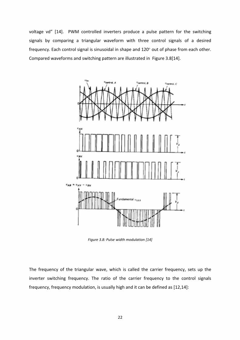
22
voltage vd” [14]. PWM controlled inverters produce a pulse pattern for the switching
signals by comparing a triangular waveform with three control signals of a desired
frequency. Each control signal is sinusoidal in shape and 120 out of phase from each other.
Compared waveforms and switching pattern are illustrated in Figure 3.8[14].
Figure 3.8: Pulse width modulation [14]
The frequency of the triangular wave, which is called the carrier frequency, sets up the
inverter switching frequency. The ratio of the carrier frequency to the control signals
frequency, frequency modulation, is usually high and it can be defined as [12,14]:
23
𝑚𝑓 =
𝑓𝑠
𝑓1 (3.12)
The output voltage of the inverter has the shape of pulses and will be rich in multiple
harmonics of the fundamental frequency. The ratio of the control signal amplitude to the
carrier signal amplitude, called the amplitude modulation ratio, can be used to predict the
RMS value of the output line to line voltage of the inverter. The amplitude modulation ratio
is defined as [12,14]
𝑚𝑎 =
𝑉𝑝 ,𝑐𝑜𝑛𝑡𝑟𝑜𝑙
𝑉𝑝 ,𝑡𝑟𝑖 (3.13)
This ratio is usually set equal to or less than 1. With this range, the line-to-line RMS voltage
across the load at the fundamental frequency can be obtained as [14]:
𝑉𝐿𝐿1 =
3
2 2𝑚𝑎𝑉𝑑𝑐 (3.14)
3.1.2.2 PWM inverter Simulation
The purpose of PWM simulation is to verify the equations listed in section 3.1.2.1. The
complete model of the inverter system has been developed using some of the existing
power electronics blocks available in the Power Library in Simulink. This includes a 3-phase
PWM IGBT inverter and a Discrete PWM Pulse Generator.
The rated power of the simulated inverter is 10 KVA and its input is an ideal DC source set at
750 V. The inverter is feeding a 9.8 KW 3 phase balanced load. Each phase of the filter
passes through a second-order, LC, low-pass filter whose parameters have been calculated
such that the cut-off frequency lies between the control signal frequency and the switching
frequency. The frequency modulation, on the other hand, was chosen to be a multiple of 3,
in order to cancel out most of the dominant harmonics in the line to line voltage as
suggested in [14]. See Table 3.9 for more details.

24
Parameter Value
Inverter rated power 10 KVA
DC source 750 V
Load voltage (L-L) 415 V RMS
Load Power 8 KW
System frequency 50 Hz
Filter Inductor ,L 2mH
Filter Capacitor, C 442 F
Carrier frequency 3000 Hz
Table 3.9: Inverter system details
In order to test the effectiveness of the designed filter system, a Total Harmonic Distortion
(THD) measurement block, which is available in Simulink, was employed to measure THD in
the inverter current. This is to ensure that the inverter complies with the requirement of
THD in Section 4.5 of Australian Standard, AS4777.2 (2005), which states that the THD of the
current shall be less than 5%. The measurement was not individually performed for single
harmonics as in Table 1 and 2 in the Standard but rather for the total harmonic [15]. The
equation used to calculate the Total Harmonic Distortion of the current is given by [16]
(THD) = IH/IF (3.15)
The numerator in equation (3.15) computes the root mean square (RMS) of the total
harmonics in the current signal as:
𝐼𝐻 = 𝐼22 + 𝐼3
2 + 𝐼42 + ⋯ + 𝐼𝑛2
Then, the obtained number is divided by the RMS value of the fundamental harmonic, 𝐼𝐹 ,
which in this case is 50 Hz. (see Appendix B for the simulation results)
Overall, the output results in Appendix B show that the inverter has been functioning as
expected i.e. the value of the amplitude modulation in Figure B.2 is exactly as calculated
from equation (3.14). The plot of THD of the current signal also confirms that the values of

25
the filter components with respect to the specified switching frequency were within the
optimal range.
3.2 Microgrid Loads
Load models consist of simple 3 phase series RL branches with constant impedances as
shown in Figure 3.10. Throughout this report it will be assumed that all loads are balanced
and in Star-grounded configuration. Loads in grid side will be disconnected by a controllable
switch when the microgrid is islanded.
Figure 3.10: Load model
3.3 Utility Grid
During the simulation of the microgrid in grid-connected mode, the grid side can be
modelled as a 3 phase power source, that is connected through distribution lines to a step-
down transformer. See Figure 3.11. The parameters of the source, transformer and
distribution lines are similar to the ones used in [17].

26
Figure 3.11: Utility grid Model.
3.4 Point of Common Coupling (PPC)
The point of common coupling can be modelled as a controllable 3 phase circuit breaker as
shown in Figure 3.12. This breaker is a time-based controllable switch that opens and closes
its contacts according to defined operation times. The reason for choosing a time-based
breaker rather than a controllable static switch, is because Simulink does not have the tools
needed to simulate the conditions described in section 2.3.5. However, the main purpose of
the switch is to simulate a transition event, and this can be achieved in either case.
Figure 3.12: Time- based circuit breaker.

27
3.5 Phase Locked Loop (PLL)
A phase locked loop is a device that generates an output signal whose phase is matched
with the phase of the input signal [5]. It is an important device used to synchronize the
microsource voltages with the grid voltage during grid-connected mode in order to prevent
the system from becoming unstable due to phase differences. During the simulation, each
microsource is equipped with a 3 phase PPL. The model of this device is available in the
power library in Simulink and it will be used frequently during the system studies. A similar
structure of this device was also found in [18]. The main components of the 3 phase PLL are
a Loop Filter (LF) and a Voltage Controlled Oscillator (VCO) as shown in Figure 3.13 [18].
Figure 3.13: 3 phase PLL block diagram [18]
3.5.1 PLL Principles of Operation
When a PLL receives the three phases voltages a, b, and c, it transforms them to the Clarke
model (see Appendix C) and then to a quadrature signal by multiplying them with internal
signals as in [18]:
Ed =E sin + E cos (3.16)

28
Inside the PLL a reference signal, 𝐸𝑑∗ , is kept at zero and compared with the synchronous
voltage component obtained in equation (3.16). The error signal is then fed to the loop
filter, which is a PI controller whose transfer function is given by:
𝐻 𝑠 = 𝐾𝑃 +
𝐾𝑖
𝑡𝑖𝑠 (3.17)
where
𝐾𝑃 proportional gain of the PI controller
𝐾𝑖 Integral gain of the PI controller
After a few loops the synchronous voltage Ed is minimized and thereby the PLL will remain
locked to the input voltages E and E and will generate a rotating reference angle, ,
synchronized with the input voltages. The Voltage Controlled Oscillator in this loop is simply
an integrator, which can be described by [18]:
H(s) = 1/s (3.18)

29
Chapter 4
4. Proposed Control Strategies for Microgrid
Operation
There are several items research carried out in the area of microgrid operation control [1,
3,7,20-25]. The control strategies for power sources within a microgrid are usually
proposed based on the required functions and the operational scenarios and they are
distinguished in their implementations between renewable energy units (non-dispatchable)
units and conventional units (dispatchable units)[3]. The focus in this chapter is only on
renewable energy sources that use power inverters to interface with AC systems. In this
case, inverters are the key components that need to be controlled in order to ensure a
stable operation of a microgrid. This can be achieved by designing a proper control scheme
that is capable of controlling the voltage, frequency and active and reactive power supplied
by the inverters. It has been also assumed that the control scheme does not rely on physical
communications between the power units. Therefore, control systems have to be designed
as a part of each microsource and independent from the other units. In general, the
appropriate control for such interfaces can be divided into two types:
- PQ inverter control
- Voltage source inverter control
The PQ inverter control can only be employed during the parallel operation of a microgrid
with the utility grid. The controller in this configuration enforces all the micro-generators to
inject a certain amount of their available power into the AC system. The set point of the
injected power for each micro-generator is pre-defined in the controller and in most cases is
100%. While the microsources inject the specified active and reactive power, PQ control
employs the voltage and frequency of the main grid as references to regulate the
microsources. The other type of control is voltage source control. This control concept is
usually implemented when the utility grid is disconnected by the monitoring controller due
to any type of power disturbances. The function of the controller in this situation is to keep
30
the voltage and the frequency of the system within the acceptable limits. It also uses the
Voltage-Reactive Power droop and Frequency-Active Power droop, that is defined in each
microsource control unit, to adjust the power sharing amongst the microsources, based on
their rated power.
4.1 Microgrid Control during Grid-connected Mode
When the microgrid is operating in parallel with the utility grid, three quantities need to be
properly controlled and maintained. They are the frequency within the microgrid, the
voltage amplitude at the connection points of the inverters to the feeder, and the power
supplied by microsources. The voltage amplitude can be simply adjusted internally by using
the PWM technique as described in section 3.1.2.1. The control system in this case uses the
amplitude of the grid voltage as a reference and generates instantaneous voltages
accordingly. The frequency of the microgrid, on the other hand, can be maintained by using
a phase looked loop (PLL) technique that synchronizes the microgrid with the utility grid.
This is done by adjusting the voltage phase angle of each inverter phase to the
corresponding phase in the grid. Therefore, the voltage and the frequency of the inverter
are indirectly controlled by the grid.
Microsources in this mode are controlled to provide specified amounts of real and reactive
power depending on the rating of the units and the energy management. Their control
schemes are designed such that units in power control configuration are operated by a
constant current controller, and units in feeder flow configuration are operated by a P-Q
controller.
4.1.1 Constant Current Control
In this type of control, the microsource unit is forced to supply a constant current output.
The control block diagram for this type is shown in Figure 4.1[17] and the details of the
controller block are shown in Figure 4.2.

31
Figure 4.1: Constant current control block diagram [17]
Figure 4.2: Details of the controller block [17]
The constant current control measures the load voltage Vabc and the inverter current Iabc
and transfers them to a DQ frame(see appendix C for the mathematical transformations ).
The PLL is used to estimate the phase angle at the microsource connection point and
generates a signal, θ (t), that rotates synchronously with the grid. The current quantities Id
and Iq are then compared with reference DC quantities Id, ref (active power set point) and Iq,ref

32
(reactive power set point) to obtain error signals. The error signals are then applied to
proportional-integral controllers to correct the errors and define the reference voltage
signals Vd,ref and Vq,ref.. Overall, this process forces the inverter to inject the defined currents
and at the same time it regulates the voltage at the connection point as measured from the
grid side. It also compensates for the voltage drops in the cable by adding their value into
the amplitude of the inverter output voltages, so that the voltage at the load is held to its
specified value.
4.1.2 P-Q Control
The block diagram of P-Q control is shown in Figure 4.3 [25]. The control structure of this
type is quite similar to the constant current control. The only difference between the two
controls is the regulated parameters, though they reach to the same conclusion, which is
output power control. In this control type, the regulated parameters are the active and
reactive powers instead of the current. Active and reactive powers are measured at the
output terminal of the inverter and then compared with the reference values to obtain the
errors. These error signals are then applied to two PI controllers in order to obtain Id, ref and
Iq,ref [25].The rest of the process is similar to the constant power technique shown earlier in
Figure 4.2.
The authors in [25] propose this control scheme to be only used for constant active and
reactive power supply. However, its implementation can be altered and it can be used for
power flow regulation in the feeder. In other words, the reference power can be defined as
the set point plus the deviation in the load demand. This is applicable for both active and
reactive power. The equations that describe the reference active and reactive power can be
written as:
𝑃𝑟𝑒𝑓 = 𝑃0 + 𝑝 ,𝑙𝑜𝑎𝑑 (4.1)
𝑄𝑟𝑒𝑓 = 𝑄0 + 𝑄,𝑙𝑜𝑎𝑑 (4.2)

33
where
𝑃0 Active power set point in the microsource control
𝑄0 Reactive power set point in the microsource control
𝑝 ,𝑙𝑜𝑎𝑑 Variation in the load active power
𝑄,𝑙𝑜𝑎𝑑 Variation in the load reactive power
Figure4.3: block diagram for P-Q control [25]
Source units that incorporate this control configuration monitor the power flow in the
feeder while supplying the set point of their active and reactive powers and if the load

34
demand increases or decreases, these units will proportionally respond by either increasing
or decreasing their supply. For instance, if a 100 KVA microsource in a typical microgrid is
controlled to inject 50% of its rated power as active power (50 KW) and 20% as reactive
power (20KVAr) and the feeder monitor detects that the active power flow is being reduced
say from 60KW to 40 KW and reactive power increased from 40 KVAr to 50 KVar, then the
regulator unit will change the output powers as follow:
𝑃𝑛𝑒𝑤 = 50𝐾𝑊 + (40𝐾𝑊 − 60𝐾𝑊)
𝑃 = 30 𝐾𝑊
𝑄𝑛𝑒𝑤 = 20 𝐾𝑉𝐴𝑟 + (50𝐾𝑉𝐴𝑟 − 40𝐾𝑉𝐴𝑟)
𝑄 = 30𝐾𝑉𝐴𝑟
By doing this, the microgrid that incorporates some microsources with similar control
configuration will be seen as fully dispatchable network since it can internally handle the
load variation without external support from the main grid.
4.2 Microgrid Control during Islanded Operation
The islanded mode of operation requires a control system that differs in its principles from
those of the grid connected mode. In this mode the microgrid has already been
disconnected from the main grid; consequently the voltage and the frequency are no longer
regulated by the grid and have to be internally controlled. In this situation, the control
system needs to accurately regulate the voltage and the frequency of the local loads. One
way to achieve this is to employ a master controller whose function is to gather and analyse
the data from both the load and the static switch and then send commands to the power
sources to adjust their powers accordingly. However, this type of controls requires physical
communications between the sources and complex software implementations. It also

35
greatly endangers the system security since a failure in the master controller will result in a
complete shutdown or an unstable operation of a microgrid. These factors, in addition to
the expensive hardware and software setup, combined to make this type of control
unattractive and imperfect to securely and reliably operate a microgrid.
The other technique is to install a control system in each microsource. The job of the
microsource controller now is to respond autonomously to system changes without
requiring any data from local loads, static switches or the other microsources. This
technique enhances the security of the system by providing back-up energy to the loads
from various microsources in case of one or more sources in the microgrid fail down. More
details on advanced developed techniques for islanded operation can be found in [1, 5, 21-
24]. Overall, the principles of the control techniques in these papers are based on the power
generators control in conventional power systems with some minor modifications. The
original design is basically a control scheme in which the value of the frequency and the
voltage are determined from what is known “voltage and frequency droop methods”. Since
the inverters are the power sources in most of the renewable energy units, their responses
to the power regulations are quite similar to conventional generators, and therefore the
conventional methods can still be used in islanded operations.
The authors in [5] propose a control method for autonomous operation of inverters which is
similar to that used in conventional power systems, see Figure 4.4. As can be seen from the
block diagram, two main blocks are used to calculate instantaneous active and reactive
powers injected by the inverter. The signals then pass through low-pass filters in order to
cancel out the higher order harmonics. After filtering the signals, the voltage and the
frequency values are determined from the Reactive Power-Voltage Droop control and the
Active Power-Frequency droop control, respectively. The voltage control block in the
diagram is simply a P-I controller that uses the stationary frame (DQ frame) quantities to
adjust the reference voltage sent to the inverter, based on the error between the measured
voltage and the desired voltage value from the Q-V characteristics.

36
Figure 4.4: Block diagram of a microsource controller [5]
This controller can function perfectly in a microgrid system where the distribution cables are
mainly inductive. In reality, such cables comprise a resistive part as well as an inductive part.
The ratio of the resistance to the inductance varies from cable to cable and it mainly
depends on the length and cross sectional area. Now consider the circuit diagram in Figure
4.5, where an inverter is supplying a load through a distribution cable. The resistance and
inductance in the cable are denoted R and L respectively. In the arrangement the active
power delivered to the load can be calculated as[22]:
𝑃 =
1
2𝜔𝐿 2+𝑅2 𝑅𝐸2 − 𝑅𝐸𝑉 cos 𝛿 + 2𝜔𝐿 𝐸𝑉 sin 𝛿 (4.3)
The supplied reactive power can also be calculated as[22]:
𝑄 =
1
2𝜔𝐿 2+𝑅2((2𝜔𝐿)𝐸2 − (2𝜔𝐿)𝐸𝑉 cos 𝛿 + 𝑅𝐸𝑉 sin 𝛿) (4.4)
where
𝜔 The angular frequency of the system in rad/s

37
𝛿 The angle power ( the angle difference between E and V)
It is clear from the previous equations that the coupling in the power flow between the
active and reactive power actually exists since the resistance and inductance values appear
in both approximations. The level of coupling can be considered as low, moderate or strong
and it is primarily determined by the R/X ratio. This makes the independent regulation of
the either active or reactive power impracticable without using decoupling techniques. One
way to avoid this is to add a virtual inductor at the interfacing inverter output as proposed
in [22]. This virtual inductance can effectively prevent the coupling between the active and
reactive power by introducing a mainly inductive impedance. The control system will then
estimate the impedance voltage drops and improve the reactive power control and sharing
accuracy without affecting the similar process for real power flow. This method can
precisely solve the power decoupling problem but at the same time it creates another
problem. In distribution cables where the ratio R/X is high, the value of the virtual
impedance has to be high as well in order to maximize the dependency of the reactive
power control on the voltage difference. By doing this, higher voltage drops will occur in the
cables and this will increase the losses in the cables, and thereby lower the performance of
the system.
E
R
Load
L
Inverter
Cable1
V
Figure 4.5: Inverter supplying a load via a distribution cable

38
Now the remaining straightforward and less complicated method is to add delay devices
whose function is to delay the instantaneous measurement of the powers. These devices
can be installed after the measurement centres of both reactive and active power and
operate by holding-up the received signals for a defined constant time. This delay can
decouple the time dependency of these parameters on each other and enhance
independent and proper control algorithms.
A modified version of the control technique in Figure 4.4 is shown in Figure 4.6. Notice that
the low pass-filters and the voltage control blocks are abandoned in the new control
version. This is to simplify the control structure and reduce the complexity of the
implementations. It is assumed that each inverter is equipped with a well designed filter
that is able to filter out all unwanted harmonics and produce pure sinusoidal waves at
specified frequency. Measurement devices were also assumed to be perfect in their
measurements and have no noise effects. The voltage control block in the original design
has an extra advantage of forcing the inverter to operate with a voltage value specified by
the P-I controller. This desired value can be actually taken directly from the reactive power-
voltage block since the inverter has to adjust its output voltage based on this frame in all
cases. Therefore, voltage control can be also neglected. Extra details for this technique can
be found in section 4.2.3.
Figure 4.6: A modified version of the control technique in [5]

39
Now with the new control scheme, the electrical parameters are measured and regulated in
their instantaneous forms and do not require the extra step of being converted to the
stationary frame components. This simplifies the equations and the overall process of the
control system.
4.2.1 P and Q Calculations
The blocks that calculate the real and reactive power use the knowledge of the
instantaneous values for the line current of the inverter and line-to-line voltage or phase
voltage at the load [5]. Under balanced and unbalanced conditions, the voltages at two
phases can be measured and the third phase will be predicated, since the sum of the three
phases is zero in all cases. This principle can also be applied to the line currents, but only
under balanced conditions.
Figure 4.7: P and Q calculation blocks
If the sensing equipments are to be kept at a minimum, so that only two phases are to be
measured, then the following equations can be used to calculate the instantaneous three
phase real and reactive powers [5]:

40
𝑃3𝑝ℎ = 𝑉𝑏𝑐 𝐼𝑐 − 𝑉𝑎𝑏 𝐼𝑎 (4.5)
𝑄3𝑝ℎ = −
𝑉𝑏𝑐 2𝐼𝑎+𝐼𝑏 +𝑉𝑐𝑎 (2𝐼𝑏+𝐼𝑎 )
3 (4.6)
If each phase is measured separately, then the following equations can be used:
𝑃3𝑝ℎ = 𝑉𝑎𝐼𝑎 + 𝑉𝑏𝐼𝑏 + 𝑉𝑐𝐼𝐶 (4.7)
𝑄3𝑝ℎ =
𝑉𝑏𝑐 𝐼𝑎 + 𝑉𝑐𝑎 𝐼𝑏+𝑉𝑎𝑏 𝐼𝑐
3 (4.8)
4.2.2 Real Power versus Frequency Droop
The Real Power Vs Frequency method to be discussed in this section is based on the
traditional control of power generators in conventional power systems. It allows
microsources to redispatch their output real power to match the load demand during the
islanded operation mode. It also performs proper sharing of real power between the units,
based on their rated powers. Figure 4.8 shows the characteristics of the real power versus
frequency droop for three power source units.

41
Figure 4.8: P Vs F characteristics for three units
From Figure 4.8, it can be noticed that each microsource has a constant negative slope
droop on the P−𝜔 plane. The coefficient of the slope is chosen to allow the frequency to
drop by a given amount as the power extends from one point to another point. When the
microgrid system operates in grid-connected mode, unit 1, 2, and 3 inject a set point of their
real power, which are denoted as P0,1 , P0,2 and P0,3 respectively. When the microgrid
system transfers to islanded mode, Ohm’s law demands larger currents from the power
sources and that will increase their measure of the output power, and as consequence of
the droop plane , the microsource will operate at a frequency slightly below the nominal
value [5]. The new power values in islanded mode are shown as Pn,1, Pn,2 and Pn,3 for units
1, 2 and 3 respectively. Now, it is clear from the graph that the characteristics of each unit
allow the real power to increase as the frequency decreases. This can be mathematically
expressed as:

42
𝑛𝑒𝑤 ,𝑖 = 0 − 𝑚𝑝 ,𝑖(𝑃𝑛𝑒𝑤 ,𝑖 − 𝑃0,𝑖)
𝑚𝑝 =
𝑃𝑚𝑎𝑥 ,𝑖 .
(4.9)
where
𝑖 Microsource unit 1,2 or 3.
0 The angular frequency of the unit when the system is connected to the grid.
𝑛𝑒𝑤 The angular frequency of the unit when the system is in islanded mode.
𝑃0 The real power supplied by the unit when the system is in grid-connected mode.
𝑃𝑛𝑒𝑤 The real power supplied by the unit when the system is in islanded mode.
𝑚𝑝 The slope of the droop characteristics.
The difference in the frequency between grid connected operation and the minimum
allowable frequency.
𝑃𝑚𝑎𝑥 Maximum power available from the unit.
Now, since the three units have the same slope constant, this method ensures that the
three units share the total real power load proportionally according to their power ratings,
while maintaining the frequency at one level.
The control block that represents the droop is shown in Figure 4.9. The block receives three
inputs: instantaneous measured power, desired power in grid-connected mode, and the
nominal frequency and it then produces the desired angle of the voltage, 𝛿𝑣 , at the inverter
bus, that is needed by the pulse generator to process the gate pulses. This angle can be
obtained by integrating the instantaneous variable 𝜔 between the limits π and –π, which in
continuous operation will have a saw tooth waveform.
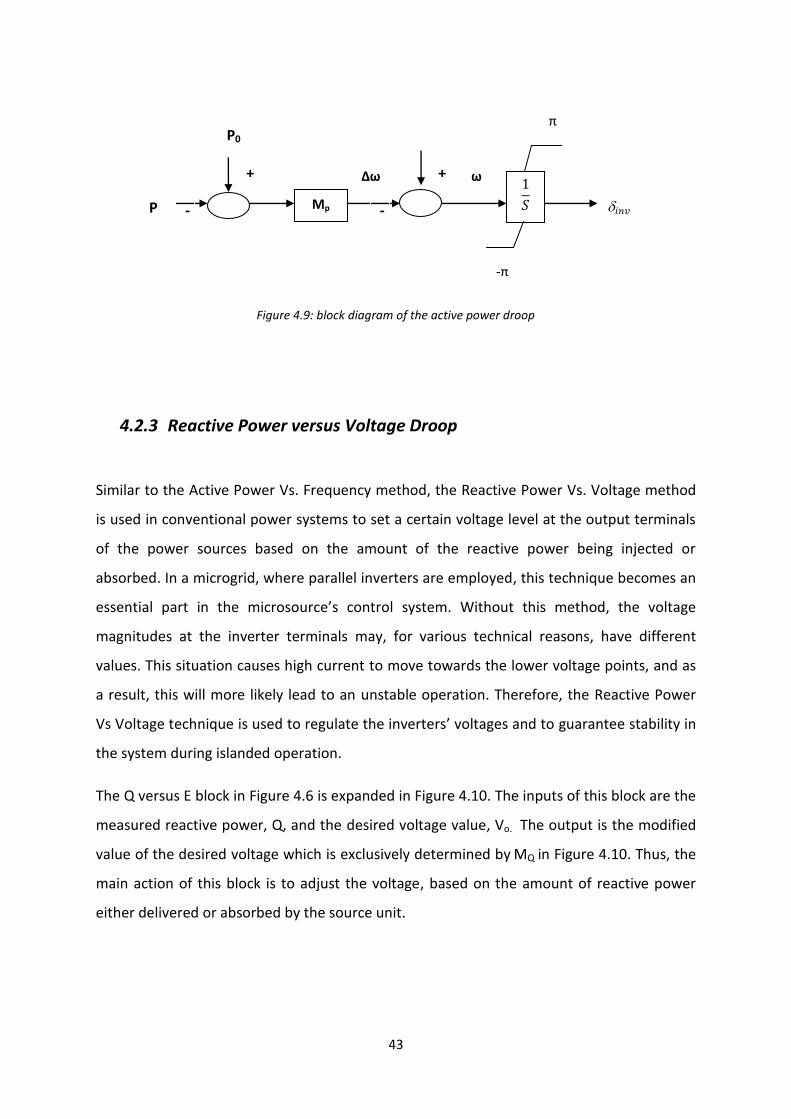
43
Figure 4.9: block diagram of the active power droop
4.2.3 Reactive Power versus Voltage Droop
Similar to the Active Power Vs. Frequency method, the Reactive Power Vs. Voltage method
is used in conventional power systems to set a certain voltage level at the output terminals
of the power sources based on the amount of the reactive power being injected or
absorbed. In a microgrid, where parallel inverters are employed, this technique becomes an
essential part in the microsource’s control system. Without this method, the voltage
magnitudes at the inverter terminals may, for various technical reasons, have different
values. This situation causes high current to move towards the lower voltage points, and as
a result, this will more likely lead to an unstable operation. Therefore, the Reactive Power
Vs Voltage technique is used to regulate the inverters’ voltages and to guarantee stability in
the system during islanded operation.
The Q versus E block in Figure 4.6 is expanded in Figure 4.10. The inputs of this block are the
measured reactive power, Q, and the desired voltage value, Vo. The output is the modified
value of the desired voltage which is exclusively determined by MQ in Figure 4.10. Thus, the
main action of this block is to adjust the voltage, based on the amount of reactive power
either delivered or absorbed by the source unit.
Mp
+
-
π
-
ω ∆ω 1
𝑆
-π
𝑖𝑛𝑣
+
P0
P
0

44
Figure 4.10: Expanded Q versus V block
Now consider a microgrid that has multiple inverters operating in parallel. The Reactive
Power Vs Voltage droop characteristic of each unit must be designed in a way that creates a
modified voltage whose set point is equal to the set points of other units in the system.
Again, this is to avoid differences in voltage magnitudes with its associated problems. Now,
since it is assumed that there is no communications between inverters, the only way to
achieve this is to place all the droop characteristics on one plane whose y-axis is
represented by the voltage and x-axis by the reactive power. This is illustrated in Figure 4.11
for three power units. On this plane maximum and minimum operating voltages are defined
based on the linear relationship between the voltage and reactive power. Each unit droop is
scaled such that the maximum reactive power injected from the unit correspond to the
minimum allowable operating voltage and the maximum reactive power absorbed by the
unit correspond to the maximum allowable operating voltage. In order to match the
voltages of different rated power units, rated power values have to be included in their
coefficients, MQ. From the plane in Figure 4.11, the operating voltage can be expressed as:
𝑉𝑖 = 𝑉0,𝑖 − 𝑚𝑄,𝑖𝑄𝑖 𝑚𝑝 =
𝑃𝑚𝑎𝑥 ,𝑖 .
𝑚𝑄 =∆V
𝑄𝑚𝑎𝑥 ,𝑖 .
(4.10)
where
𝑖 Microsource unit 1,2 or 3.
𝑉 Operating voltage .
MQ
Q E
-
+ ∆V
V0

45
𝑉𝑜 Nominal voltage value.
𝑄 The reactive power injected or absorbed by the microsource (negative value if the unit is
absorbing reactive power).
𝑚𝑄 The slope of the droop characteristics.
∆𝑉 The difference in the voltage between the nominal value and the maximum/minimum
value.
𝑄𝑚𝑎𝑥 Maximum reactive power from the microsource.
Notice that in equation 4.10 the operating voltage will be equal to the requested nominal
voltage if the unit is neither injecting nor absorbing reactive power. However, in a situation
where the unit is injecting reactive power, the operating voltage will be less than the
nominal voltage and it will be higher if the reactive power is being absorbed. It can also be
observed that the regulation of the voltage requires variation in the reactive power supply,
since the voltage and the reactive power have a linear relationship. For multi sized power
units, this variation is proportional to the size of the unit, and consequently the reactive
power of the load will be shared evenly between the power units according to their sizes.
Figure 4.11: Reactive power Vs voltage droop characteristics for 3 units
46
Chapter 5
5. Simulation Platform
5.1 Matlab Simulink
Matlab Simulink is a powerful package for modelling, simulating and analysing an
extraordinarily wide range of physical and mathematical systems. These systems include
linear and non-linear systems, and in the Simulink environment they can be modelled in
continuous or discrete times. What makes Simulink an attractive and relatively easy
software tool is that it provides the users with a series of graphical block diagramming tools
and a set of block libraries that help in completely designing and testing a wide range of
time-varying systems. It also allows the integration of dynamic blocks, which require a set of
defined transfer functions and differential equations, alongside with the electrical
component blocks within the same frame.
5.2 Tested Microgrid Structure
For the purpose of study and investigation of the proposed control schemes and strategies,
a low voltage microgrid system which represents a small power supply network in
residential areas has been designed. The single line diagram of this system is shown in
Figure 5.1.

47
Figure 5.1: Tested microgrid structure
In this system all the microsources and loads are in 3-phase Y-g configuration. Two of the
loads are sensitive and must be continuously supplied even after the loss of the main grid.
The third load is non-critical and therefore will ride through the disconnection event.
Throughout the investigation, loads will be treated as 3 phase balanced loads, and therefore
there is no need for a phase voltage compensator. For the operating voltage and frequency,
the tolerated ranges will be 2405% for the phase voltage and 501 Hz for the system
frequency. In reality, the constraint on the limits may vary in some situations due to a
number of technical and economic factors, but, in the simulation stage, the voltage and

48
frequency will be restricted within the defined ranges as stated in [15] for the inverter
requirements.
The circuit breaker (CB) in the system will operate to isolate or reconnect the microgrid
when it is required. The conditions that trigger isolation can be defined as any situation in
which voltage, frequency or current in the main grid goes beyond the acceptable limits.
However, due to the difficulties in simulating such situations in Simulink, the circuit breaker
is modelled as a time-based isolator which gives the user the full control to isolate or
reconnect the microgrid from the main grid at any specified times.
The proposed microgrid system incorporates three microsources with different rated
powers. The reason for including three microsources in the structure is to study the load
sharing principles, since the control techniques in the previous chapter were described for a
variable number of microsources and loads. The biggest microsource is a PV unit that
interfaces with the system through an inverter whose rated power is 50 KVA. The second
and third units are also PV systems and their inverters are sized 25 KVA and 10 KVA
respectively. Each microsource is connected to the common bus through a cable with a
unity X/R ratio, since it is assumed that the cable length is a few hundred meters. The actual
size of the inductance and resistance in the cables is derived from the size of the inverter to
which the cable is connected. This is suggested in [5] for better operation performance. P
and Q plane capability with constant voltage and impedance analysis had been performed in
that report, and it was found that each value of cable inductance defines a certain region
that limits the delivery of active and reactive power. Cable impedance with 0.2 pu was
realized to be the best region over which the supplied powers can reach P=1 p.u and Q=0.75
p.u with an inverter voltage of 1.12 p.u and a power angle of 10 degrees.
The main utility grid is represented by a 20 kV distribution network model using a simple R-L
equivalent for the distribution lines, Ls and Rs. The microgrid is integrated into the grid via a
100 kVA, three-phase, 50Hz, 20/0.415 kV -Yg transformer. More details for the system
parameters and cable calculations can be found in Appendix D.

49
5.3 Implementation in Simulink
The implementation of the microgrid structure in Simulink is shown in Figure E.1 in
Appendix E. All the elements of the single line diagram in Figure 5.1 were replaced by their
corresponding dynamic models. The models for all standard electrical components like
transformers, voltage sources, and loads were adopted from the Powerlib toolbox in
Simulink. The other blocks, which include transfer functions and integrators, were obtained
from the main library.
The PV system and the inverter, that were modelled in chapter 3, can be combined with the
control system to form a complete model for a microsource. However, when simulating a PV
system with an inverter, the DC-link voltage of the prime mover needs to be considered
[26]. This voltage has to be maintained at specified value in order to obtain a reference
power delivered to the inverter from the PV system side. The configuration is illustrated in
Figure 5.2.
Figure 5.2: DC-link capacitor power balance
Assuming that the capacitor is ideal, the power balance in the capacitor of the DC-link can
be instantaneously calculated by subtracting the power delivered by the PV system, PPV, and
the power received from the inverter, Pinv. The relationship can be mathematically expressed
as:
𝑃𝐶 = 𝑃𝑃𝑉 − 𝑃𝑖𝑛𝑣 (5.1)
The power delivered by the capacitor in the DC-link can also be expressed as:

50
𝑃𝐶 = 𝑉𝐷𝐶 ∗ 𝐼𝐷𝐶
∗ (5.2)
where 𝑉𝐷𝐶 is the capacitor voltage and 𝐼𝐷𝐶
∗ is the capacitor current. Now, from equation (5.2)
it is clear that the DC-link can be maintained at a specified reference by regulating the
power balance in the DC-link. Combining equation (5.1) and (5.2), to give:
𝑉𝐷𝐶 ∗ 𝐼𝐷𝐶
∗ = 𝑃𝑃𝑉 − 𝑃𝑖𝑛𝑣 (5.3)
The relationship between the capacitor voltage and the capacitor current is given by
𝑉𝐷𝐶 =
1
𝐶 𝐼𝐷𝐶
∗ 𝑑𝑡 (5.4)
where C is the capacitance value in the DC-link. Again, combining equation (5.2) and (5.4)
and taking the Laplace transform of both sides, the DC -link can be modelled as shown in
Figure 5.3 [26].
Figure 5.3: Dynamic model of a DC-link [26]
The model obtained for the DC-link can be placed between the PV system and the inverter
to define a set point for the microsource power based on the reference current and the
capacitance value. It is a relatively simple technique that does not require complicated
blocks in its implementation. However, the simulation time associated with this model and
the inverter model can sometimes be extremely long. It is an aim that the simulation time

51
span does not exceed one minute per run, but with the detailed microsource in Simulink this
will take several minutes. It is also suggested in [27] that the detailed inverter modelling
should be avoided when analysing the dynamic behaviour of a microgrid and it is better to
represent the inverters’ long term dynamic models by their control functions. This means
that the transients related to the communication of solid-state switches in the inverters are
not considered. Additionally, this technique assumes that the AC power injected from the
inverters is without harmonics, distortions or losses. If the inverter transient is to be
studied, then full modelling is required.
Since the study objectives in this thesis ask only for analysis of the overall microgrid dynamic
behaviour and not for the microsource in particular, the microsource can be simplified to a
model that responds to the commands from the controllers based on their control functions
as suggested in [27]. The variables in these functions are only power, voltage, and
frequency. The new model for the microsource is shown in Figure 5.4.
Figure 5.4: Microsource model represented by its control functions
𝑆𝑖𝑛 𝑢
𝑆𝑖𝑛 𝑢 −2𝜋
3
𝑆𝑖𝑛 𝑢 +2𝜋
3
×
×
×
From Q Vs V droop
From P Vs ω droop
Ua
V,max
Ub
Uc
δinv

52
Now, all microsource models in Figure 5.1 only consist of an inverter model similar to the
one in Figure 5.4 and a control system. The complete control scheme for both autonomous
and grid-connected modes is given in Figure E.2 of appendix E.

53
Chapter 6
6. Simulation Results
In order to evaluate the performance of the proposed power control strategies, a significant
number of simulated experiments have been carried out in Matlab/Simulink. The simulation
was performed on the 3 phase low-voltage microgrid given in Figure 5.1. The simulation
parameters for this system can be found in Tables F.1 and F.2 in Appendix F. In this chapter,
four typical operational scenarios are considered. These are as follows:
Scenario A): the microgrid operates in parallel with the main grid and the three
microsources are in unit power control configuration (UPC configuration).
Scenario B): the microgrid operates in parallel with the main grid and the
microsources are in a mixed configuration.
Scenario C): the microgrid switches from grid-connected mode to islanded mode .
Scenario D): the microgrid operates in islanded mode.
A. Microgrid Operates in Grid-Connected Mode with UPCC
In this scenario, it is assumed that the transfer switch at the PCC is closed and all
microsources are in UPC configuration. The initial power references for all microsources
were set at 0.8 p.u in the form of active power only; the load reactive power demand is
supplied by the main grid ( Idref set to 0.8 and Iqref set to 0). Notice that the set point of the
reference power can vary from 0 to a maximum of 1 p.u for both active and reactive power,
since the control systems were designed to operate the microsource at any power level, but
with a condition that the combined powers (active and reactive) do not exceed the rated
power of the microsource. Therefore, power set points and load values in this section and
later sections were randomly chosen in order to only examine the designed control system
responses i.e. they are not based on energy management studies.

54
While the microsources inject 80% of their available power as real power, the total load,
including the non-sensitive load, was initially set at 40KW and 15 KVAr. At time 0.1s the load
variation is applied and the load increased by 60KW and 20 KVAr. Figure 6.1 shows the
microsource power outputs, load demands, feeder flows in the grid side, and system
frequency over a period of 0.3 s.
(a)
(b)
(c)
0 0.05 0.1 0.15 0.2 0.25 0.3
0
0.5
1
1.5
2
2.5
3
3.5
4
4.5
x 10
4
0 0.05 0.1 0.15 0.2 0.25 0.3-1
-0.5
0
0.5
1
1.5x 10
4
0 0.05 0.1 0.15 0.2 0.25 0.3
-11
-10
-9
-8
-7
-6
-5
-4
-3
-2
-1
x 10
4
P (
W)
Q (
VA
r)
Load
(P
,Q)
P1
P2
Q1=Q2=Q3=0
Load Q
Load P
P3

55
(d)
(e)
Figure 6.1: Simulation results for scenario A – all microsources operate in UPC mode. (a) Real power output of
each microsource. (b) Reactive power output of each microsource. (c) Load active and reactive power demands.
(d)Total power flow in the grid feeder. (e) System frequency
As can be seen in Figure 6.1(a) and 6.1(b), the microsources output powers tracked the
reference values very well. They injected the desired real power and left the reactive power
of the load supplied by the grid. It can also be noticed that the microsource powers
remained constant throughout the simulation, despite the variation of the load. The
variations of the load in both active and reactive powers were totally compensated by the
grid. This proves that the designed control system for the grid-connected mode is capable of
totally dispatching the inverter currents independently from the load demand.
0 0.05 0.1 0.15 0.2 0.25 0.3
-5
-4
-3
-2
-1
0
1
2
3
4
x 10
4
0 0.05 0.1 0.15 0.2 0.25 0.349.975
49.98
49.985
49.99
49.995
50
50.005
50.01
50.015
FL(P
,Q) Q flow
P flow
F (H
z)

56
The structure of the tested microgrid system allows the power exchange between the main
grid and the microgrid. At time before 0.1s the total real power generated by the
microsources exceeds the load’s need, and as a result, the extra real power was transferred
from the microgrid to the main grid. Power flows in the grid feeder are shown in 6.1(d),
where the negative sign implies that the grid is receiving power from the microgrid. This
demonstrates one of the microgrid benefits on the utility grid, i.e. when the generated
power exceeds the local load, the microgrid can act as an active power system which may
help the main grid to share external loads during peak times.
As mentioned in chapter 4, voltage and frequency during the grid-connected mode are
controlled by the grid. From the result in Figure 6.1 (e), it can be said that the PLL
implemented in Simulink was successful in synchronizing the microgrid system with the
main grid. The common bus voltages in p.u and a phase voltage in (V) are shown in Figure
6.2.
(a)
0 0.05 0.1 0.15 0.2 0.25 0.3
-1.5
-1
-0.5
0
0.5
1
1.5
2
Vab
c (p
.u)

57
(b)
Figure 6.2: Simulation results for scenario A – all microsources operate in UPC mode. (a) Instantaneous
voltages in p.u at the common bus. (b) Load phase voltage in V at the common bus
B. Microgrid Operates in Grid-Connected Mode with a Mixed
Configuration
In this scenario, the microgrid is still in grid-connected mode but with a mixed configuration.
Microsource1 (MS1) and microsource3 (MS3) are employed to regulate their output power
(installed in unit power control configuration) whereas microusource2 (MS2) is used to
monitor and regulate the power flow in the feeder (installed in feeder flow control
configuration). The power references of the microsources at this time were set at 1 p.u for
MS1 and MS3, again as real power only. The set point of MS2 was initially put at 0.45 p.u.
However, since MS2 is installed in feeder flow control configuration, its output power is
variable and it depends on the power flow in the feeder. The purpose of this microsource is
to adjust its operation according to the variation in the load, such that the power in the
feeder stays constant. This can be achieved by either increasing its output if the load
increases or reducing the power if the load decreases.
In order to simulate this situation and test whether MS2 can track load variation, the total
load was initially set at 70 KW and 20 KVAr. At time 0.1s the load was increased by 10 KW
and 0.1s after this is increased by 5 KVAr. It was then changed and settled at 60 KW and
0 0.05 0.1 0.15 0.2 0.25 0.3-400
-300
-200
-100
0
100
200
300
400
Va
(v)

58
15KVAr at t=0.3s. Simulated results for microsource powers and feeder powers are given in
Figure 6.3.
(a)
(b)
(c)
Figure 6.3: Simulation results for scenario B. (a) Real power output of each microsource. (b) Reactive power
output of each microsource. (c) Power flows in the grid feeder.
The simulation results indicate that MS2 responded well to the step changes in load active
and reactive powers. When the load increased by 10 KW at 0.1s, MS2 detected a change in
the power flow in the feeder and reacted very quickly to compensate the load. Similarly,
0 0.05 0.1 0.15 0.2 0.25 0.3 0.35 0.4-1
0
1
2
3
4
5
6x 10
4
0 0.05 0.1 0.15 0.2 0.25 0.3 0.35 0.4
-1.5
-1
-0.5
0
0.5
1
x 10
4
0 0.05 0.1 0.15 0.2 0.25 0.3 0.35 0.4
0.5
1
1.5
2
2.5
3
3.5
x 10
4
P1
P2
P3
Q2
P (
W)
Q (
VA
r)
FL(Q) FL(P) FL(P
,Q)
Q1=Q3=0

59
when the load reactive power increased at time 0.2s, the extra demand was picked up by
MS2. At time 0.3s when both load active and reactive power changed, MS2 again adjusted
its output powers accordingly. It reduced its output active power to minimum and started
absorbing reactive power in order to balance the power flows in the feeder. The controller
of MS2 in this situation uses the voltage magnitude and the phase angle at the inverter
output terminals to regulate the power flows from or into the inverter. In reactive power
regulation, for example, the controller forces a certain value of voltage magnitude at the
inverter terminal in order to satisfy the set point, which is the difference in the reactive
power flow in the feeder. To illustrate this, the 3 phase voltages at the MS2 output terminal
are zoomed and pasted in Figure 6.4 below. It can be seen that at the time when MS2 was
requested to inject reactive power, the controller raises the inverter voltage magnitude to a
point that allows it to inject the commanded set point of the reactive power. On the other
hand, when the MS2 was required to absorb reactive power, the controller decreased the
inverter voltage magnitude, and therefore made it seem like a reactive power load to the
grid.
Figure 6.4: MS2 terminal voltages
Overall, microgrids with microsources having mixed configurations can offer the best
solution to the grid in the area of significant load variation problems. That is, besides
reducing the load on the utility by serving their local loads, microgrids ensure that the
0 0.05 0.1 0.15 0.2 0.25 0.3 0.35334
336
338
340
342
344
346
348
350
352
Vo
ltag
e (V
)
Q=0
Injecting Q
Absorbing Q

60
power from the grid stays constant under changing load conditions. This arrangement
makes the microgrid a truly dispatchable load as seen from the utility side.
C. Microgrid Switches from Grid-Connected Mode to Islanded
Mode
Initially the transfer switch was closed, and all the microsources were operating in UPC
configuration. During grid-connected mode, their output powers were controlled to be 0.5
p.u in the form of real power and 0.2 p.u in the form of reactive power. At time 0.1s, the
transfer switch turned ON to isolate the microgrid from the grid, and then these
microsources were operating in islanded mode. After 0.1s from the disconnection, the
system was reconnected back to the grid. The total of the two sensitive loads was set at 60
KW and 30 KVAr, and the non-sensitive load was set at 40 KW and 15 KVAr. It is obvious that
the total load inside the system is higher than the available power from all microsources,
and therefore load shedding on the non-sensitive load was applied when the system
transferred to islanded mode. Figure 6.5 shows the simulation results for the microsource
output powers, MS1 currents in p.u, load shedding, grid powers, and the system frequency.
(a)
0 0.1 0.2 0.3 0.4 0.5 0.6 0.7 0.8 0.9 1
-3
-2
-1
0
1
2
3
4
5
6
x 10
4
P(w
)
P1
P2 P3
P2

61
(b)
(c)
(d)
0 0.1 0.2 0.3 0.4 0.5 0.6 0.7 0.8 0.9 1-2
-1
0
1
2
3
4
5x 10
4
0 0.05 0.1 0.15 0.2 0.25 0.3
-1
-0.5
0
0.5
1
0 0.1 0.2 0.3 0.4 0.5 0.6 0.7 0.8 0.9 1-12
-10
-8
-6
-4
-2
0x 10
4
Q(V
Ar)
C
urr
ent
(p.u
) Lo
ad p
ow
er (
P,Q
)
Q1 Q2 Q3
Load P (W)
Load Q (VAr) L3 reconnection L3 shedding

62
(e)
(f)
Figure 6.5: simulation results for scenario C – all microsources operate in UPC mode. (a) real power output of
each microsource. (b) reactive power output of each microsource. (c) MS2 current in p.u. (d) load powers. (e)
grid powers. (f) system frequency.
Simulation results show that during grid-connected modes the MS’s pursued their
references as specified for both active and reactive power and extra load demand was
supplied by the grid. When the microgrid transferred to islanded mode, the load sharing
between MS’s was achieved and all MS’s increased their powers to match the load demand.
The output changes, as expected, almost in proportion to their ratings. The system
frequency in this mode dropped and settled at 49.3 Hz. This is not shown in Figure 6.5 (f)
0 0.1 0.2 0.3 0.4 0.5 0.6 0.7 0.8 0.9 1
-4
-2
0
2
4
6
8
10
12
14
x 10
4
0 0.1 0.2 0.3 0.4 0.5 0.6 0.7 0.8 0.9 1
49.5
49.6
49.7
49.8
49.9
50
50.1
50.2
Gri
d p
ow
er (
P,Q
) F
(Hz)
Grid P (W)
Grid Q (VAr)

63
since the system did not have the time to reach steady state. On the other hand, during the
grid-connected modes, the PLL was precisely able to synchronize the microgrid with the grid
at 50 Hz.
The significant oscillations that appear on the power plots, particularly in islanded mode, are
due to the snubber circuit in the transfer switch. In Simulink, such circuit have to be defined
in the power switches if the switches are connected in series with inductive circuits. It
simply consists of a resistor and a capacitor in series, connected in parallel with the switch.
Its job is to suppress overshot in the voltage when the inductive load is disconnected from
the power supply. However, due to its arrangement with the system, this circuit creates a
moderate resonance level in the microgrid, which is caused mainly by the effect of charging
and discharging of reactive power between the snubber capacitor and the inductive load.
D. Microgrid Operates in Islanded Mode
The response of proper sharing controller in accordance with load changes in islanded mode
will be investigated in this scenario. It was assumed that the microgrid is operating in steady
state and the total sensitive load is 40 KW and 25 KVAr. The grid model, transfer switch, and
non sensitive load were removed from the system to speed up the simulation time and
eliminate the resonance effects. At time 1s the real power and reactive power of the load
increased by 20 KW and 5 KVAr respectively. MS’s powers, load demands, MS1 current in A,
the voltage at the common bus, and the system frequency are shown in Figure 6.6.

64
(a)
(b)
0 0.5 1 1.5 2 2.5 30
0.5
1
1.5
2
2.5
3
3.5
x 10
4
0 0.5 1 1.5 2 2.5 30
2000
4000
6000
8000
10000
12000
14000
16000
18000
P(W
) Q
(VA
r)
P2
P1
P3
Q1
Q2
Q3

65
(c)
(d)
0 0.5 1 1.5 2 2.5 3-6
-5
-4
-3
-2
-1
0x 10
4
0 0.5 1 1.5 2 2.5 30.95
0.955
0.96
0.965
0.97
0.975
0.98
0.985
0.99
0.995
1
Load
(P,Q
) V
olt
age
(p.u
)
LoadP (W)
Load Q (VAr)
0.968 p.u
0.961 p.u

66
(e)
(f)
Figure 6.6: Simulation results for scenario D – all microsources operate in islanded mode. (a) real power output
of each microsource. (b) reactive power output of each microsource. (c) load demands. (d) common bus
voltage in p.u. (e) MS1 phase current in A. (f) system frequency.
As noticed in the simulation results of this scenario, the droop techniques perfectly
distributed the load powers between the microsources according to their ratings. At time
before 1s real power delivered was 24KW, 12.5KW, and 5KW from MS1, MS2, and MS3 and
the reactive power was 14.5KVAr, 7.3KVAr and 3KVAr from MS1, MS2 and MS3
0 0.5 1 1.5 2 2.5 3-80
-60
-40
-20
0
20
40
60
80
0 0.5 1 1.5 2 2.5 349.2
49.3
49.4
49.5
49.6
49.7
49.8
49.9
50
Cu
rren
t (A
) F(
Hz)

67
respectively. When the load increased by 20 KW and 5KVAr at time 0.2s, the microsources
increased their output powers and picked up the extra load in a proportional manner.
Unlike the controller in grid-connected mode, the controller in this mode allows for voltage
variation and frequency deviation at the load as explained in section 4.2. The variation of
the voltage from nominal value is based on the amount of reactive power being delivered or
absorbed from microsources. In the case when the microgrid is serving a capacitive load, the
voltage at the common bus will be higher than the nominal value and it will be lower when
the load is inductive. The latter case is illustrated in Figure 6.6(d). The steady state voltage at
the common bus was around 0.968 p.u when load demanded 25KVAr and eventually settled
at 0.961 p.u when the total reactive power was set at 30 KVAr. On the other hand, the
system frequency had been greatly affected by the variation in the load real power. Initially,
the load real power was almost half the total of microsource ratings and according to the
designed P-w plane, the system frequency has to be in the middle of the defined allowable
limits. From Figure 6.6 (f), the initial value of system frequency was 49.49 Hz which is close
to the theoretical value calculated using equations in section 4.2 i.e. 49.53 Hz. The reason
for such discrepancy between simulation result and calculated value is that the
microsources had to inject more power than what was needed from the load to compensate
for losses in the system cables, and this would slightly lower the frequency operating point
on the plane. Overall, it can be noticed that both voltage and frequency cannot exceed their
allowable ranges, since they were defined with the maximum rating of each microsource
and they will reach the edge of their limits only in a the case where the microsources
operate at their rate powers.
68
Chapter 7
7. Conclusion and Suggestions for Future Work
In this final chapter the importance and the main outcomes of the thesis research are
highlighted and summarized. It also contains some suggestions for future work in both the
area of microgrid control and the area of microgrid modelling.
7.1 Thesis Conclusion
This thesis intended to examine the microgrid concept and to suggest control strategies that
can reliably and efficiently operate a balanced 3 phase low-voltage microgrid in grid -
connected and islanded modes. At the first stage of this thesis, and in order to study and
analyse the behaviour of a microgrid, the essential components in a typical microgrid
system were modelled. Although some of the components were not fully modelled, the
operation of combined components gave a useful insight into the dynamic behaviour of a
full microgrid under various load conditions, particularly when implementing control
strategies. Furthermore, control strategies that are needed for microgrid islanded and grid-
connected operations, with an assumption that there is no communication between the
microsources, were also described and evaluated in this report. The technique used to
control the microgrid during islanded mode was based on the conventional system
approaches for voltage and frequency regulation in addition to load sharing enhancement
between generators. From the analysis performed on the simulation results, it can be said
that the conventional droop methods can be effectively employed to control the operation
of parallel inverters coupled by low R/X cables, since they have proven their robustness and
effectiveness in regulating frequency and voltage during islanded operation. Their power
sharing principles were also examined, and the simulation results indicated that all

69
microsources in the tested system shared the proper amount of power via these methods,
while keeping the voltage and the frequency within the acceptable limits. For the operation
of a microgrid during grid-connected mode, constant current control and P-Q control
schemes were introduced and explained. These two schemes have proven their robustness
in regulating the output powers from all microsources as specified in the references and the
Phase Locked Loop was always able to accurately synchronize the microgrid with the grid.
Additionally, these two schemes have also successfully achieved a pure decoupling between
real power and reactive power when the microgrid was operating in grid-connected mode,
as shown in the simulation results. The microsource configurations linked with these two
control types were also tested in this thesis. It was found that a microgrid with mixed
configuration makes the best operational state in which the overall efficiency of the
microgrid is maximized and the load variation impact on the grid is minimized.
7.2 Suggestions for Future Work
As mentioned previously, one of the thesis objectives was to model a complete microgrid
system. The goal was to study its behaviour in a bigger picture without getting involved with
detailed dynamic modelling. This approach achieved the objective very well. However, the
suggestion for the next step is to include full dynamic details for all components, particularly
the prime movers and inverters, in order to validate the results and investigate the
interaction between the sources on one side and between the sources and the grid on the
other side. It is also recommended to extend the range of the microsources by including
various renewable energy systems (e.g. wind turbines, fuel cells) and then study how they
react with each other.
It is must be pointed out that only control strategies for balanced systems were addressed
in this project. Unbalanced voltages can greatly affect the stability and the operation of a
microgrid. Furthermore, other phenomena, such as voltage sags and harmonic distortion
associated with inverters, can impact the microgrid operations as well. Thus, further studies
in these areas are highly recommended.

70
Storage devices are one of the essential parts in a typical microgrid. These devices were not
considered in this project. It is suggested to include their models in future work in order to
study their benefits as back-up sources and to examine their operation when working in
parallel with microsources, as well as investigating their charging/discharging phenomena.
Since inductance and resistance values in transmission cables determine the level of
coupling between active and reactive powers, system stability analysis over a wide range of
R/X ratios is strongly recommended. This may sometimes require a modification to the
droop methods and an accurate P-I controller tuning.
Finally, a hardware laboratory setup for a small scale microgrid is needed in order to
disprove or confirm the simulation results.
71
8. References
1. Li, Yunwei, Mahinda Vilathgamuwa, and Poh Chiang Loh. 2004. Design, Analysis and
Real-Time Testing of a Controller for Multibus Microgrid System . IEEE Transactions
on Power Electronics, VOL. 19, NO.5. September (2004): 1195-1203.
2. S. Chowdhury, S.P. Chowdhury, and P. Crossley. 2009. Microgrids and Active
Distribution Newtwork . London: Institution Of Engineering And Technology.
3. Katriraei, Farid , Reza Iravani, Nikos Hatziargyriou, and Aris Dimeas.2008. Microgrids
Management: Control and Operation Aspects of Microgrids. IEEE power and energy
magazine, May /June 2008. Pages: 54-65
4. Kroposki, Benjamin , Robert Lasseter, Toshifumi Ise, Satoshi Morozumi, Stavros
Papathanassiou, and Nikos Hatziargyriou. 2008. Making Microgrids Work. IIEEE
power & energy magazine, May /June 2008. Pages: 40-53
5. Robert H. Lasseter and Paolo Piagi. 2006. Control and Design of Microgrid
Components. University of Wisconsin-Madison.
6. Piagi, Paolo , and Robert H. Lasseter.2006. Autonomous Control of Microgrids. IEEE
PES Meeting, Montreal, 2006.
7. Ahn, Seon-Ju , Jin-Woo Park, Il-Yop Chung, Seung-Il Moon, Sang-Hee Kang, and
Soon-Ryul Nam. 2010. Power-Sharing Method of Multiple Distributed Considering
Control Methods and Configurations of a Microgrid. IEEE TRANSACTIONS ON POWER
DELIVERY, VOL. 25, NO. 3, JULY (2010): 2007-2016.
8. Anca D. Hansen, Poul Sorensen, Lars H. Hansen, and Henrik Bindner. 2000. Models
for a Stand-alone PV System. Roskilde: Riso National Laboratory.
9. R. Sudharshan Kaarthik, Nayan Kumar Dalei, R. Vigneshwaran and Rabinarayan
Das. 2010. Modelling, Simulation and Implementations of Low Power Photovoltaic
Energy Conversion System. Bachelor Thesis, National Institude of Technology
Rourkela.
10. Faisal A. Mohamed. 2008. Microgrid Modelling and Online Management. PhD Diss.,
Helsinki University of Technology.
11. JIN-WOO JUNG. 2005. PROJECT #2 SPACE VECTOR PWM INVERTER. DEPARTMENT
OF ELECTRICAL AND COMPUTER ENGINEERING.

72
12. Muhammad H. Rashid. 2004. Power Electronics: Circuits, Devices and
Applications.3rd ed. Alexandria, VA: Prentice Hall.
13. Iqbal, Atif, Adoum Lamine, Imtiaz Ashra, and Mohibullah shaleh.2006.
Matlab/Simulink Model of Space Vector PWM for Three-Phase Voltage Source
Inverter. Universities Power Engineering Conference, UPEC '06. Proceedings of the
41st International (2006): 1096-1100.
14. Ned Mohan, Tore M. Undeland, and William P. Robbins. 2003. Power Electronics
converters application and design. 3rd ed. Hoboken: John Wiley & Sons, Inc.
15. Australian Standard 4777.1. 2005. Grid Connection of energy Systems Via Inverters:
Installation Requirements.
16. Measure Total Harmonic Distortion (THD),
http://www.mathworks.com/help/toolbox/physmod/powersys/ref/totalharmonicdi
stortion.html accessed on 10/09/2010
17. M. Popov, H. Karimi, H. Nikkhajoei and V. Terzija. Dynamic Model and Control of a
Microgrid with Passive Loads. http://www.ipst.org/techpapers/2009/papers/20.pdf
. Accessed on 22/08/2010
18. Rym Marouani and Abdelkader Mami. Voltage Oriented Control Applied to a Grid
Connected Photovoltaic System with Maximum Power Point Tracking Technique.
http://www.scipub.org/fulltext/ajas/ajas781168-1173.pdf, accessed on 13/08/2010.
19. Deng, Jiamei , Shuangbao Ma, and Yong Xue.2009. Power Flow Control of a
Distributed Generation Unit in Micro-Grid. Power Electronics and Motion Control
Conference, IPEMC '09. IEEE 6th International : 2122 - 2125 .
20. Basak, Prasenjit , A. K. Saha, S. Chowdhury, and S. P. Chowdhury. 2009. Microgrid:
Control Techniques and Modeling. Universities Power Engineering Conference
(UPEC), 2009 Proceedings of the 44th International : 1-5.
21. Hiskens, Ian A., and Eric M. Fleming. 2008. Control of Inverter-Connected Sources in
Autonomous Microgrids. American Control Conference (2008): 586 – 590
22. Wei Li, Yun , and ChingNan Kao.2009. An accurate power control strategy for
inverter based distributed generation units operating in a low voltage microgrid.
Energy Conversion Congress and Exposition, ECCE 2009 (2009): 3363 - 3370 .
23. I. VECHIU, A. LLARIA, O. CUREA1 and H. CAMBLONG. Control of Power Converters for
Microgrids”. http://cmrt.centrale-

73
marseille.fr/cpi/ever09/documents/papers/re4/EVER09-paper-181.pdf, accessed on
11/08/2010
24. Majumder, Ritwik, Farhad Shahnia, Arindam Ghosh, Gerard Ledwich, Michael
Wishart, and Firuz Zare. 2009. Operation and control of a microgrid containing
inertial and non-inertial micro sources. TENCON 2009 - 2009 IEEE REGION 10
CONFERENCE 44 (2009): 1 – 6
25. R. S. Alabri and E. F. El-Saadany. Interfacing Control of Inverter-based DG Units.
http://icccp.net/proceedings/2009/Papers/ICCCP09-076.pdf , accessed on
22/08/2010.
26. Carlos Coelho Leal Moreira. 2008. IDENTIFICATION AND DEVELOPMENT OF
MICROGRIDS EMERGENCY CONTROL PROCEDURES. PhD Diss., University of Porto,
2008.
27. A.P. Lopes, C.L. Moreira, and F.O. Resende. 2005. Microgrids black start and
islanded operation.
http://www.montefiore.ulg.ac.be/services/stochastic/pscc05/papers/fp69.pdf, accessed
on 13/10/2010

74
9. Appendices
9.1 Appendix A
PV Panel Modelling and Simulation
The following equations are taken from [8] and applied for the PV panel whose parameters
are in [10]
The net current generated by a PV cell can be calculated as:
𝐼 = 𝐼𝑝ℎ − 𝐼𝐷
= 𝐼𝑝ℎ − 𝐼𝑜 exp𝑒 𝑉+𝐼𝑅𝑠
𝑚𝐾𝑇𝐶− 1
where
𝑚 Idealizing factor
𝐾 Boltzmann’s constant (1.38 ∗ 10−23𝐽/𝐾)
𝑇𝐶 Absolute temperature of the cell
e Electronic charge (1.602 ∗ 10−19𝐶)
V The imposed voltage across the cell
𝐼𝑜 The Dark saturation current
Total current injected by a PV panel can is given by:
𝐼𝑚 = 𝑁𝑃𝐼𝑆𝐶𝑐 [1 − exp(
𝑉𝑚 − 𝑁𝑆 𝑉𝑂𝐶𝑐 +
𝐼𝑚𝑅𝑆𝑐
𝑁𝑃
𝑁𝑆𝑉𝑡𝑐)
where

75
𝐼𝑚 Module current
𝑉𝑚 Module voltage
𝑁𝑃 Number of cells in parallel
𝑁𝑆 Number of cells in Series
𝐼𝑆𝐶𝑐 Cell short circuit current
𝑉𝑂𝐶𝑐 Cell open circuit voltage
𝑉𝑡𝑐 Cell thermal voltage, 𝑉𝑡𝑐 =𝑚𝐾𝑇𝑐
𝑒
The short circuit current can be computed based on a linear dependency on the solar
radiation:
𝐼𝑠𝑐𝑐 = 𝐺𝑎
The open circuit voltage of the cell depends on the operating temperature:
𝑉𝑜𝑐𝑐 = 𝑉𝑜𝑐 ,𝑜
𝑐 + (𝑇𝑐 − 𝑇𝑐0)
where
𝑉𝑜𝑐𝑐 the open circuit voltage of a cell at a certain operating condition
Open circuit voltage temperature coefficient (= -78.2mV/C from Table 3.2)
𝑇𝑐 working temperature of the cell
𝑇𝑐0 cell temperature at the standard condition, 25 C.
The operating temperature of the cell, 𝑇𝑐 , can be computed using the following equation:
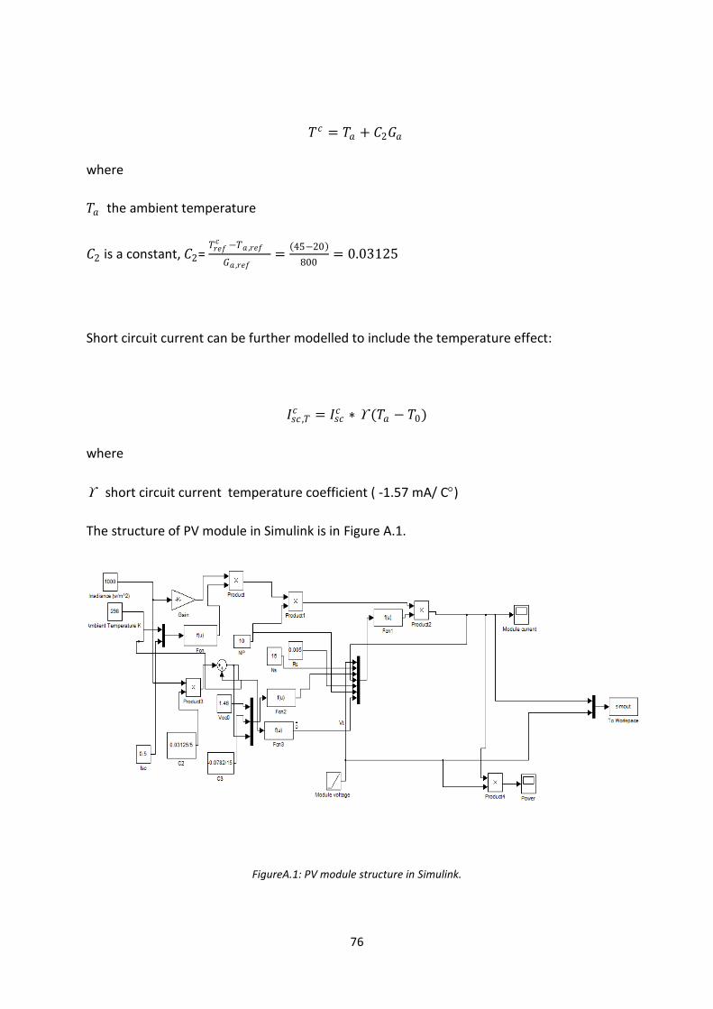
76
𝑇𝑐 = 𝑇𝑎 + 𝐶2𝐺𝑎
where
𝑇𝑎 the ambient temperature
𝐶2 is a constant, 𝐶2= 𝑇𝑟𝑒𝑓𝑐 −𝑇𝑎 ,𝑟𝑒𝑓
𝐺𝑎 ,𝑟𝑒𝑓 =
45−20
800= 0.03125
Short circuit current can be further modelled to include the temperature effect:
𝐼𝑠𝑐 ,𝑇𝑐 = 𝐼𝑠𝑐
𝑐 ∗ (𝑇𝑎 − 𝑇0)
where
short circuit current temperature coefficient ( -1.57 mA/ C)
The structure of PV module in Simulink is in Figure A.1.
FigureA.1: PV module structure in Simulink.

77
9.2 Appendix B
3- ph inverter simulation
The structure of the inverter system in Simulink is shown in Figure B.1.
Figure B.1: Inverter system structure in Simulink
Plots of DC voltage, inverter line to line voltage, Vabc of the load in per unit, Iabc of the
inverter in per unit, Phase b voltage of the load , and the modulation index over a period of
0.4 seconds are shown in Figure B.2.

78
Figure B.2: Inverter simulation results.
The line current of the inverter as well as its total harmonic distortion are shown in Figure
B.3.
Figure B.3: Inverter line current and THD.
Inverter line current (A)
THD in the inverter voltage

79
9.3 Appendix C
Mathematical Transformation
Voltage and current can be transformed from abc form to the stationary two-axis reference
frame (- frame) as follows, where X denotes either voltage or current
𝑋
𝑋
𝑋0
= 2
3
1 −
1
2−
1
2
0 3
2−
3
21
2
1
2
1
2
𝑋a
𝑋b
𝑋𝑐
And from stationary two-axis reference frame to rotating two-axis reference frame (DQ
frame) as follows:
𝑋d
𝑋q
𝑋0
= 2
3
cos 𝑤𝑡 sin 𝑤𝑡 0− sin 𝑤𝑡 cos 𝑤𝑡 0
0 0 1
𝑋
𝑋
𝑋0
Instantaneous quantities, abc, can be also transformed to DQ mode using the following
matrix:
𝑋d
𝑋q
𝑋0
= 2
3
cos 𝑤𝑡 cos(𝑤𝑡 −
2
3𝜋) cos(𝑤𝑡 +
2
3𝜋)
− sin 𝑤𝑡 −sin(𝑤𝑡 −2
3𝜋) −sin(𝑤𝑡 +
2
3𝜋)
1
2
1
2
1
2
𝑋a
𝑋b
𝑋𝑐

80
And from DQ model back to abc model using the inverse relationship which can be
expressed as:
𝑋a
𝑋b
𝑋𝑐
= 2
3
cos 𝑤𝑡 – sin 𝑤𝑡
1
2
cos(𝑤𝑡 −2
3𝜋) −sin(𝑤𝑡 −
2
3𝜋)
1
2
cos(𝑤𝑡 −2
3𝜋) −sin(𝑤𝑡 +
2
3𝜋)
1
2
𝑋d
𝑋q
𝑋0
Active power in DQ model can be calculated using the following equation:
𝑃 = 𝑉𝑑𝐼𝑑 + 𝑉𝑞𝐼𝑞
And the reactive power can be expressed as:
𝑄 = 𝑉𝑑𝐼𝑞 − 𝑉𝑞𝐼𝑑

81
9.4 Appendix D
Tested System Details
1. Cable inductance and resistance calculations
The equation for the base quantities can be written as:
𝑆𝑏𝑎𝑠𝑒 = 3 𝑉𝑏𝑎𝑠𝑒 𝐼𝑏𝑎𝑠𝑒
𝑍𝑏𝑎𝑠𝑒 =𝑉𝑏𝑎𝑠𝑒
𝐼𝑏𝑎𝑠𝑒 ∗ 3=
𝑉𝑏𝑎𝑠𝑒2
𝑆𝑏𝑎𝑠𝑒
Unit 1:
Inverter rated power, Sbase = 50 KVA
System base voltage, Vbase = 415 V L-L
𝑍𝑏𝑎𝑠𝑒 =415𝑉2
50𝐾𝑉𝐴= 3.445
Since the inductance and resistance values chosen to be 0.2 p.u, the inductance in the each
of the three cables can be obtained as:
𝐿1 = 0.2 ∗𝑍𝑏𝑎𝑠𝑒
3 ∗ (2𝜋𝑓)= 0.2 ∗
3.445
3 ∗ (2𝜋50)= 0.73 𝑚𝐻
The ratio of R/X is 1, therefore the value of the resistance will be :
𝑅1 = 0.2 ∗3.445
3= 0.229
Unit 2:
Inverter rated power, Sbase = 25 KVA
System base voltage, Vbase = 415 V L-L

82
𝑍𝑏𝑎𝑠𝑒 =415𝑉2
25𝐾𝑉𝐴= 6.889
With similar calculation performed for unit 1 , the inductance in these inverter’s cables will
be :
𝐿2 = 0.2 ∗6.889
3 ∗ (2𝜋50)= 1.462𝑚𝐻
And the resistance value is
𝑅2 = 0.2 ∗6.889
3= 0.46
Unit 3:
Inverter rated power, Sbase = 10 KVA
System base voltage, Vbase = 415 V L-L
𝑍𝑏𝑎𝑠𝑒 =415𝑉2
10𝐾𝑉𝐴= 17.22
The inductance value in the cables is :
𝐿3 = 0.2 ∗17.22
3 ∗ (2𝜋50)= 3.66 𝑚𝐻
And the resistance value is
𝑅3 = 0.2 ∗17.22
3= 1.148

83
2. Transformer Parameters
Parameter Value
Rated Power 100 KVA
Primary Winding
Rated Voltage 11 KV
Resistance 0.002 p.u
Inductance 0.09 P.u
Winding connection Secondary Winding
Rated Voltage 240 V
Resistance 0.002 p.u
Inductance 0.09 P.u
Winding connection Y-g
Magnetizing branch
Resistance 1700 p.u
Inductance 2000 p.u
Table D.1: Transformer parameters
Resistance and inductance values for a winding are given in p.u. based on the transformer
rated power and the rated voltage of that winding. Magnetizing branch values are referred
to the primary winding.

84
9.5 Appendix E
Implementation in Simulink
The implementation of the proposed microgrid system in Simulink is shown in Figure E1.
Figure E.1: Tested microgrid structure in Simulink
The complete control scheme for each microsource is shown in Figure E.2. Notice that the
upper control blocks, that include the droops coefficients, are for the islanded operation

85
and the lower blocks are for the grid-connected mode. The control for either operation is
brought to action by using the time based switches (TBSs) whose operation is controlled by
using external timer.
Figure E.2: complete control scheme for each microsource

86
9.6 Appendix F
Simulation Parameters
i. Simulation Parameters for Islanded operation control
Unit Parameter Value
Unit 1
Rated power (KVA) 50
Constant time of P decoupling (s)
0.1
Constant time of Q decoupling (s)
0.2
mP (rad/s/w) 1.256E-4
mQ (V/VAr) 2.4E-4
0 (rad/s) 314
V0 (Vrms) 240
Unit 2
Rated power (KVA) 25
Constant time of P decoupling (s)
0.1
Constant time of Q decoupling (s)
0.2
mP (rad/s/w) 2.512E-4
mQ (V/VAr) 4.8E-4
0 (rad/s) 314
V0 (Vrms) 240
Unit 3
Rated power (KVA) 10
Constant time of P decoupling (s)
0.1
Constant time of Q decoupling (s)
0.2
mP (rad/s/w) 6.28E-4
mQ (V/VAr) 1.2 E-3
0 (rad/s) 314
V0 (Vrms) 240
Table F.1: Simulation parameters during autonomous mode

87
ii. Simulation Parameters for Grid-Connected Control
The parameters listed in Table E.4 are same for all microsources control systems
Device Parameter Value
3-ph PLL Regulator gain (Kp) 10
Regulator gain (Ki) 100
PID controller for real power Proportional gain (Kp) 10
Integral gain (Ki) 20
Derivative gain (Kd) 0
PID controller for reactive power
Proportional gain (Kp) 10
Integral gain (Ki) 20
Derivative gain (Kd) 0
Table F.2 : Control parameters for grid-connected operation