methods to identify and prioritize deer locations.pdfdvc/mile to identify hotspots, ... gaps, the...

METHODS TO IDENTIFY AND PRIORITIZE DEER VEHICLE CRASH LOCATIONS – FINAL REPORT

Prepared for The Federal Highway Administration

1200 New Jersey Avenue, SE. Washington, D.C 20590

Prepared by NORMANDEAU ASSOCIATES, INC.

25 Nashua Road Bedford, NH 03110

R-19977.002

June 2011

Task 4 Final Report

TABLE OF CONTENTS

Table of Contents ................................................................................................................................. ii

List of Appendix C Figures................................................................................................................. iv

List of Tables......................................................................................................................................... v

1.0 Introduction...............................................................................................................................1

2.0 Background...............................................................................................................................2

3.0 Summary of Current Practice..................................................................................................3

4.0 Assessment Methods to Identify Hotspots............................................................................6

5.0 Data ............................................................................................................................................7 5.1 Data Sources ....................................................................................................................7 5.2 Data Processing ...............................................................................................................7

6.0 Methods .....................................................................................................................................8 6.1 Clustered or not Clustered?..............................................................................................8

6.1.1 Nearest Neighbor..................................................................................................8 6.1.2 Moran’s I ...............................................................................................................9

6.2 Where are the Hotspots?..................................................................................................9 6.2.1 Visual Analysis....................................................................................................10 6.2.2 Density-Based Analysis ......................................................................................11 6.2.3 Modeling .............................................................................................................12 6.2.4 Spatial Statistics .................................................................................................13 6.2.5 Expert Opinion ....................................................................................................14

7.0 Results.....................................................................................................................................15 7.1 Iowa I-35 .........................................................................................................................16 7.2 Iowa Route 65.................................................................................................................17 7.3 New York I-90 .................................................................................................................18 7.4 New York Route 28.........................................................................................................19

8.0 Comparison of Methods ........................................................................................................20 8.1 Underlying Distribution....................................................................................................20 8.2 Hotspot Methods.............................................................................................................20 8.3 Choosing a Method.........................................................................................................23

9.0 Predicting DVC Locations .....................................................................................................24

10.0 Conclusion and Recommendations .....................................................................................25

11.0 References ..............................................................................................................................26

Appendix A – Literature Review..........................................................................................................1

1.0 Introduction........................................................................................................................... A-5

2.0 Identifying DVC Hotspots .................................................................................................... A-5 2.1 Non-Quantitative Methods............................................................................................ A-6 2.3 Traditional Statistics...................................................................................................... A-8 2.3 Spatial Statistics ........................................................................................................... A-9

ii Normandeau Associates, Inc.

Task 4 Final Report

3.0 Methods to Examine the Relationship of DVCs to Roadway and Environmental Factors ................................................................................................. A-9

4.0 Factors Associated with DVC Hot Spots.......................................................................... A-10

5.0 Predicting DVC Locations ................................................................................................. A-12

6.0 Sources of Data for DVC Analysis .................................................................................... A-13

7.0 Literature Cited ................................................................................................................... A-15

Literature Review: Appendix A ..................................................................................................... A-17 Cited References Summarized in Tabular Format by Topic Area........................................ A-17

Appendix B – Summary of Current Practices................................................................................ B-1 Questions Asked During Interviews of Dot Safety and Environmental Personnel ................. B-5

Appendix C - Figures ....................................................................................................................... C-1

iii Normandeau Associates, Inc.

Task 4 Final Report

LIST OF APPENDIX C FIGURES

Appendix Figure C-1. Iowa Locus Map................................................................................................C-2

Appendix Figure C-2. New York Locus Map. ......................................................................................C-3

Appendix Figure C-3. Comparison of map types for visual analysis. .................................................C-4

Appendix Figure C-4. Density Based Analysis – comparing thresholds based on mean DVC/mile to identify hotspots, IA Rt 65...........................................................C-5

Appendix Figure C-5. Route 65 hotspots identified using a binomial model (95% CI) and a three-mile moving window based on the binomial model. .............................C-6

Appendix Figure C-6. CrimeStat Results – Route 65, illustrating variation in results based on number of DVC considered and size of search radius used. A color-coded visual analysis map is provided for comparison. .................................C-7

Appendix Figure C-7. Data (map) used for the expert analysis, Iowa Route 65................................C-8

Appendix Figure C-8. Iowa I-35 Results. Figure 8a segments are labeled by DVC count; all others are labeled by segment number. .........................................................C-9

Appendix Figure C-9. Iowa Route 65 Results. 9a segments are labeled by DVC count; all others are labeled by segment number. .......................................................C-10

Appendix Figure C-10. New York I-90 Results. 10a segments are labeled by DVC count; all others are labeled by segment number. .......................................................C-11

Appendix Figure C-11. NY Route 28 Result. 11a segments are labeled by DVC count; all others are labeled by segment number. .......................................................C-12

iv Normandeau Associates, Inc.

Task 4 Final Report

v Normandeau Associates, Inc.

LIST OF TABLES

Table 1. Summary of interview results relating to analysis of DVC hotspots. States are sorted by name of the DOT branch that conducts DVC hotspot analysis............................5

Table 2. Hotspot analysis methods assessed under Task 4...............................................................6

Table 3. Summary of data from each study area. ...............................................................................7

Table 4. Data needs and software used for each assessment method considered. .......................10

Table 5. Number and proportion of segments identified as hotspots by each method....................15

Table 6. Overlap of segments identified as hotspots.........................................................................15

Table 7. Comparison of analysis methods assessed under Task 4. ................................................22

Task 4 Final Report

1.0 INTRODUCTION

The Deer-Vehicle Crash Information and Research (DVCIR) Center is a multi-state pooled fund project which also includes the Federal Highway Administration (FHWA) as the lead agency. The State Departments of Transportation (DOTs) that fund the DVCIR Center activities are Connecticut, Iowa, Maryland, Minnesota, New Hampshire, New York, Ohio, Texas, and Wisconsin. In order to fill methodological knowledge gaps, the DVCIR commissioned the Investigation of Methods to Identify and Prioritize Deer-Vehicle Crash Locations of Concern. The over arching goal of the project is to help participating states evaluate and advance their deer vehicle crash (DVC)-related safety management system. To meet this goal, the main objectives of the investigation were to:

OBJECTIVES

Document and evaluate the existing crash analysis approaches, capabilities, and/or DVC-related databases along with best practices

Summarize the different approaches and tools

Evaluate the application of several selection/prioritization methodologies

Document and evaluate the existing crash analysis approaches, capabilities, and/or DVC-related databases of participating pooled fund states along with the “best practices” in these subject areas from throughout the United States, including any examples of DOT safety programs that systematically combined the use of roadway and land characteristic databases in their decision-making.

Summarize the different approaches and tools that could be used to identify and prioritize DVC hot spot locations and analyze DVC data.

Evaluate the application of several selection/prioritization methodologies at case study locations and describe their advantages and disadvantages.

DEFINED

DVC Hotspots: Locations where DVC are the most intensely clustered or where more DVCs occur than are expected by chance .

Additionally, the DVCIR was interested in the use of the identified methodologies and tools for predictive purposes. The typical approach to “hot spot” location identification is reactive in nature, i.e., crashes need to occur and be recorded before improvement. Examining the available analysis methods for use in a prediction/modeling or pro-active identification of new roadway segments that have the potential to be DVC hot spots is also in issue of interest.

To meet the main objectives of the project, the investigation was broken into three primary tasks:

Literature review – the primary goal of this task was to identify the full range of methods available to identify DVC hotspots. Additionally, the literature was examined to identify variables associated with DVC hotspots and any methods currently used to predict likely DVC hotspots, based on their association with these variables.

Survey Current practice – personnel from 24 DOTs were interviewed to identify the most common, as well as the range, of methods currently used to identify general vehicle crash and DVC hotspots for safety purposes. Additionally, interviewees were asked about data sets used to supplement and/or confirm non-roadway factors believed to impact DVCs, and if they were aware of any current practices documented to reduce DVCs and/or improve the efficiency and quality of DVC data collection.

Evaluate Methods and Tools – the goal of this task was to evaluate the advantages and disadvantages of methods currently available for use by state DOTs to locate and prioritize DVC hotspots, using a desktop analysis based on existing DVC data.

The third objective of the investigation is the main focus of this report. Results of the literature review are however incorporated in to the methodological assessment to provide context to the assessment decisions, and a brief overview of the current practice survey is also included. The complete results of these two tasks are provided in Appendices.

1 Normandeau Associates, Inc.

Task 4 Final Report

2.0 BACKGROUND

In many states DVCs are significant in number and widespread. Like other types of crashes, however, there are often particular roadway segments where clusters or “hot spots” of DVCs occur. These roadway segments need to be properly identified and prioritized in a systematic manner for effective and efficient implementation of potential DVC countermeasures. This is especially true because the area- or system-wide implementation of current DVC countermeasures is not generally considered to be economically feasible.

THE CHALLENGE

DVC “hotspots” need to be properly identified and prioritized in a systematic manner for effective and efficient implementation of potential DVC countermeasures.

DVC hotspots can be indentified using the methods that safety personnel use to identify locations where an excessive number of all types of crashes occur over time. DOT safety personnel have traditionally used density measures based on standard distributions, sometimes in combination with a sliding windows approach, to identify crash hotspots. However, this approach is prone to error, due to the inherent variability and non-normalcy of crash data (Persuad, 2001).

CURRENTLY

DOT safety personnel have traditionally used density measures based on standard distributions, sometimes combined with a sliding windows approach

Ecologists employed a variety of methods, some which are similar to those used by safety personnel, some which are novel.

Ecologists studying the interactions of deer with highways have also employed a variety of methods to identify DVC hotspots (Appendix A), some of which are the same or similar as those used by safety personnel, and some of which are novel. However, they have not generally used statistically rigorous or mathematically appropriate approaches to identify hotspots either. An additional issue that is also rarely addressed by either safety personnel or ecological researchers, is how best to chose the values of the user-specified criteria that are part of any analysis process. “User-specified criteria” include decisions about study area size and thresholds for a hotspot to be considered significant.

Approaches that are more mathematically correct for the type of data being analyzed, and that offer some degree of guidance for choosing the values of user specified criteria are available, and are being adopted for application by some DOTs. In addition to the programs initiated by a few individual states, the new SafetyAnalyst tool (2009) developed by the FHWA also uses a mathematically appropriate modeling approach to identify collision hotspots, and may be poised to become more widely used among DOTs for analysis of general collision hotspots. However, the results of the survey of current practice (Section 3; Appendix B) indicated the majority of DOTs do use more “traditional” approaches. Although there is no clear explanation for this finding, some historic reasons may include:

Safety personnel come from diverse backgrounds, and few appear to have a math/stat background.

Lack of tools (software) – until recently most software solutions required proficiency with complex statistical packages or advance programming skills. Many users may be unaware of the reasonably user friendly tools that are currently available.

Lack of computing power – modern desk top computers have largely solved this problem.

Although the diversity of background dealing with safety issues is unlikely to change, lack and computing power is no longer a problem. Easy to use of-the-shelf software tools are abundant, and many have the advantage of being open-source and cost-free to use. However, this does lead to the new problem of identifying the most appropriate tool for the question at hand. The results of this investigation provide guidance for solving this important issue.


Task 4 Final Report

3.0 SUMMARY OF CURRENT PRACTICE

For the survey of current practice, 24 states were chosen for a phone interview to gather information regarding if and how states currently identify DVC hotspots. The results of the surveys are summarized in Table 1, and the full report from this task is available in Appendix B.

SURVEY STATE BY STATE

24 states chosen for phone interview

16 have some type of DVC Hot spot analysis

Eight states do no formal DVC hotspot analysis

Of the states surveyed:

16 states did some type of DVC hotspot analysis. The responsibility for analysis was split between:

• Safety branches (eight states)

• Environmental branches (six states)

• Fish and Wildlife Departments (FWD; two states)

Environmental Branches/FWDs: States that gave the analysis responsibility to their Environmental branches or FWDs were predominantly located in the western US, where deer populations have well-defined migration routes.

• All the western states contacted for the surveys have developed or are developing state-wide wildlife and habitat linkage analyses, in cooperation with state natural resources agencies and environmental NGOs.

• The linkage maps created from these analyses provide the primary tool for identifying DVC hotspot locations in these states, augmented to varying degrees with crash data from the Safety branches, and carcass location data from various sources.

• In all cases, the analyses to identify DVC hotspots conducted by the Environmental branches were visually based, consisting of mapping the DVCs and/or carcasses, then overlying them with linkage maps. Project-specific analyses might also include expert opinion, and some consideration of traffic volume.

Safety Branches: Of the eight Safety branches that conducted analyses to identify DVC hotspots, Maine, Iowa, and Ohio had formal programs, while the remaining five conducted analysis informally and/or at the request of districts.

• A variety of analysis methods were used, including visual analysis of mapped data, and comparisons of frequency or rate over a section.

• Maine, Ohio, and Alabama used the same approach with DVC that they used with other types of crashes, but the other five states used a less rigorous approach with their DVC data, as compared to their general crash data.

• The contacts at Georgia, Iowa, and Nebraska all indicated that their analysis had revealed DVC to be largely random, and that it was difficult to identify DVC hotspots.

No Analysis: Seven states located in the East and Upper Midwest and Texas do no formal identification analysis for DVC hotspots (Table 1).

• Two of these states (Illinois, Wisconsin) remove deer crashes from their analysis of general crash hotspots because they believe DVC to be random.

• Additionally, informal analysis of DVC data conducted in North Carolina indicates that DVC appear to be randomly distributed.

• However, despite a belief that DVC occur randomly, all three of these states indicated that they do believe DVC are a significant safety issue.


Task 4 Final Report


• Two states (New Hampshire, Minnesota) noted that DVC may be identified as the primary contributor to a crash hotspot during general hotspot analysis.

Note: None of the states indicating that DVC appeared to be randomly distributed reported using statistical tests that formally define DVC distributions as random, even, or clustered. The value of implementing formal tests to identify patterns that meet the statistical definition of random or clustered is discussed in subsequent section s of this report.

In Summary

The DVC-related databases of the surveyed state were comprised primarily of DVC locations extracted from the general crash databases maintained by each DOT’s Safety Branch. Some DOTs augmented there crash data with carcass data (e.g., Colorado, Iowa, Utah, Washington,) or were developing carcass data bases for future use (e.g., New York). Maryland had the most developed carcass program, with enough spatially accurate carcass locations recorded to conduct reliable analyses of DVC distributions and hotspot locations. The only non-roadway data source used by DOTs in DVC hotspot analysis that was identified in the survey were the state-wide wildlife and habitat linkage maps, created in cooperation with state natural resources agencies and environmental NGOs in some western States (Arizona, California, Colorado, Idaho, Washington).

None of the States that were interviewed had assessed the effectiveness of either their DVC hotspot identification program or the countermeasure program in terms of DVC reduction. Maine is currently undertaking assessment of countermeasures, but sample sizes are still too small to draw conclusions. This lack of critical assessment makes it difficult to identify “best practices”. However, the programs in western states that had access to State-wide wildlife linkage maps and the programs with a formalized analysis approach (Maine, Iowa, Ohio) to conducting yearly state-wide assessment for DVC hotspots were also the programs that explicitly stated that DVC considerations were being incorporated in to their State’s roadway project planning and design. Linkage mapping efforts and formal DVC analysis programs appeared to either create or be a product of institutional acceptance that DVC considerations should be a part of project and safety planning.

Task 4 Final Report


Table 1. Summary of interview results relating to analysis of DVC hotspots. States are sorted by name of the DOT branch that conducts DVC hotspot analysis.

State* Who does

DVC Analysis?

DVC Hotspot Method In-house

Biologist?

Habitat Linkage

Program?

Non-Roadway Factors Considered?

Mitigation Program?

ID DNR Expert opinion No Yes Linkages Fencing, underpasses

WA DNR Visual Yes Yes Linkages Fencing, underpasses

AZ Enviro ? Yes Yes Linkages Fencing, underpasses

CA Enviro Visual, expert opinion Yes Yes Linkages Fencing, underpasses

CO Enviro Visual Yes Yes Topo, migration routes Fencing, underpasses

MD Enviro Visual No No Topo, vegetation Signage

NY Enviro Visual Yes No Food sources Awareness campaigns

UT Enviro Visual Yes Yes Migration routes Fencing, underpasses

CT NA NA No No NA Informal

FL NA NA No No NA No

IL NA NA No No NA No

MN NA NA No No NA Signage

NC NA NA No No NA Awareness campaigns

NH NA NA No No NA No

TX NA NA Yes No NA Signage

WI NA NA No No NA Awareness campaigns

AL Safety Frequency No No No Local

GA Safety Frequency No No No No

IA Safety Visual No No No Fencing

ME Safety Visual No No Wintering locations Various

NB Safety Frequency No No No Signage, veg control

OH Safety Rate, frequency, density No No Vegetation Awareness campaigns, veg control

PA Safety Rate No No No Fencing, awareness

VA Safety Visual No No No Signage

*States in Bold are Pooled Fund states.

Task 4 Final Report

4.0 ASSESSMENT METHODS TO IDENTIFY HOTSPOTS

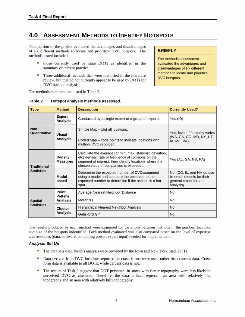
This portion of the project evaluated the advantages and disadvantages of six different methods to locate and prioritize DVC hotspots. The methods tested included:

BRIEFLY

The methods assessment evaluated the advantages and disadvantages of six different methods to locate and prioritize DVC hotspots.

those currently used by state DOTs as identified in the summary of current practice

Three additional methods that were identified in the literature review, but that do not currently appear to be used by DOTs for DVC hotspot analysis.

The methods compared are listed in Table 2.

Table 2. Hotspot analysis methods assessed.

Type Method Description Currently Used?

Expert Analysis

Conducted by a single expert or a group of experts. Yes (ID)

Non-Quantitative Visual

Analysis

Simple Map – plot all locations.

Coded Map – code points to indicate locations with multiple DVC recorded.

Yes, level of formality varies (WA, CA, CO, MD, NY, UT, IA, ME, VA)

Density Measures

Calculate the average (or min, max, standard deviation, etc) density, rate or frequency of collisions on the segment of interest, then identify locations where the chosen value of comparison is exceeded.

Yes (AL, GA, NB, PA)

Traditional Statistics

Model-based

Determine the expected number of DVCs/segment using a model and compare the observed to the expected number to determine if the section is a hot spot.

No (CO, IL, and NH do use binomial models for their general crash hotspot analysis)

Average Nearest Neighbor Distance No Point Pattern Analysis Moran’s I No

Hierarchical Nearest Neighbor Analysis No

Spatial Statistics

Cluster Analysis Getis-Ord Gi* No

The results produced by each method were examined for variations between methods in the number, location, and size of the hotspots indentified. Each method evaluated was also compared based on the level of expertise and resources (data, software, computing power, expert input) needed for implementation.

Analysis Set Up

The data sets used for this analysis were provided by the Iowa and New York State DOTs.

Data derived from DVC locations reported on crash forms were used rather than carcass data. Crash form data is available to all DOTs, while carcass data is not.

The results of Task 3 suggest that DOT personnel in states with flatter topography were less likely to perceived DVC as clustered. Therefore, the data utilized represent an area with relatively flat topography and an area with relatively hilly topography.


Task 4 Final Report

5.0 DATA

5.1 DATA SOURCES

DVC data were acquired from the Iowa and New York State DOTs, and are summarized in Table 3.

The data were provided in a GIS ready format, and each DVC in the data set had an x, y coordinate that allowed it to be located in space and mapped.

Both states provided GIS data layers that represented the roadway network where the DVC data had been collected. Two roadway segments, a limited access multi-lane highway and an unlimited access state highway, of about 50 miles each were chosen from both states for analysis.

Only the primary roadways were considered for analysis, no side roads or on/off ramps were included in the study areas.

Beyond the intentional inclusion of different highway and topography types, the locations and datasets chosen for analysis were not screened before hand for any particular attributes.

The two Iowa study areas covered a 48-mile long segment of I-35 and a 51-mile long segment of Rt 65 in Cerro Gordo and Franklin Counties (Figure C-1). The DVC data were collected from 2004 through 2009.

The two New York study areas covered a 50 mile stretch of I-90 and a 50-mile segment of Rt 28 in Oneida, Herkimer, and Hamilton Counties (Figure C-2). The DVC data were collected from 2000 through 2009.

Table 3. Summary of data from each study area.

State Road Study Area Size

(miles) Total DVC

Average DVC/Mile

Range Standard Deviation

I-35 48 287 5.98 0-16 3.52

Iowa Route 65 51 252 4.94 0-27 4.93

I-90 50 218 4.36 0-9 2.34

New York Route 28 50 122 2.44 0-6 1.86

5.2 DATA PROCESSING

The New York data were not provided with an attribute table that identified crashes by the year of occurrence. These data had to be analyzed as a 10-year data set, and for consistency, the Iowa data were not subdivided by year. ArcView was used to process the data into a usable format.

Each roadway line was buffered by 1000 meters to create a polygon that represented the road.

The polygon was segmented into multiple mile-long polygons or segments, and the number of DVC that occurred in each segment counted.

The DVC/segment count was added to the attribute table that represented the segment data layer.

The DVC/segment was then used to generate simple descriptive statistics for each study area (Table 3) and as the metric of comparison and feature value for the visual, density-based, and spatial analyses.


Task 4 Final Report

6.0 METHODS

Two Types of Analysis Methods Examined

1) Methods to examine how DVC are distributed along a roadway, i.e., are they randomly distributed, evenly distributed or clustered; and

2) Methods to identify DVC “hotspots,” i.e., locations where DVC are the most intensely clustered. ANALYSIS TASKS &

SOFTWARE

Process Data: ArcView

Create Maps: ArcView

Density- & Model-Based Cluster Calculations: Excel

Spatial Methods: ArcView, CrimeStat

Generate Input Parameters for the Model-Based Analysis: Matlab

As noted above, ArcView was used to process the data and also to create all maps.

Calculations for the density-based and model-based cluster analyses were conducted using Excel.

The spatial statistic capabilities in ArcView and CrimeStat were used for the spatial methods (Moran’s I, Getis-Ord GI*, and hierarchical nearest neighbor).

Matlab was used to generate input parameters for the model-based analysis.

The six methods examined, consisting of one approach to determine the underlying distribution of points in space and five approaches to identify hotspots, are describe briefly below.

6.1 CLUSTERED OR NOT CLUSTERED?

Objects, features, and events can be distributed in space evenly, randomly, or in clusters. Spatial statistics have been developed specifically to examine patterns among points distributed in space, and determine their underlying distribution. Spatial statistics can also be used to identify any patterns in the values associated with those points.

6.1.1 Nearest Neighbor This approach is offered by both ArcView and CrimeStat. For a nearest neighbor distance (NND) analysis, the distances between each point and its x nearest neighbors are measured and then all the distances are averaged. If the average distance is less than the average for the hypothetical random distribution, the distribution of the points being analyzed are considered clustered. If the average distance is greater than a hypothetical random distribution, the features are considered dispersed.

Software Limitations

Most software packages are designed to calculate a hypothetical random distance for points distributed across a two-dimensional area, not along a one-dimensional line, and are therefore not appropriate for DVC data. Instead, a linear nearest neighbor analysis must used, and this option does not appear to be available in most spatial statistics packages as spatial statistics have generally been developed to work with two-dimensional areas.

Software Solutions

Alternatively, using programming language and/or available extensions, it is possible to script a linear nearest neighbor routine in ArcView that will apply points randomly to a line, then measure the distance between points by following the line only, and calculate the average NND (Barnum 2003, Clevenger et al. 2008). This script can then be used as the basis for a Monte Carlo simulation (see Section 5.2.1) to determine an accurate average NND for the DVCs.

Other readily available “canned” software methods suitable for linear data are available to examine the inherent clustering and provide a less complex implementation. Assuming that most users would prefer “canned” approach, the NND approach was not a carried forward for this analysis.


Task 4 Final Report

6.1.2 Moran’s I Moran’s I evaluates whether the values associated with a collection of points are expressed in a clustered, dispersed, or random pattern (i.e., are high and low values clustered with like values, or are they mixed together in either a random or regular pattern?).

The test calculates the Moran's I index value for each location of interest, based on a user input search radius (distance band).

A Z-score and p-value are then calculated to express the significance of that index value.

Because the size of the search radius will affect the outcome, it is recommended that multiple distance bands be tested and the results inspected to determine at what scale, if any, clustering is most apparent.

The ArcView version of Moran’s I as a method that evaluates spatial autocorrelation based on the null hypothesis which is stated as “there is no spatial clustering of the values associated with the points of interest.” The Moran’s I test allows the user to input search radii of choice and compare the outcomes to determine at what scale, if any, clustering appears to be most intense. For this analysis, all study areas were evaluated for clustering using distance bands of 2, 4, 8, 12, and 16 miles. The results are discussed by study area in Section 6.0.

MORAN’S I

In statistics, Moran's I is a measure of spatial autocorrelation developed by Patrick A.P. Moran. Spatial autocorrelation is characterized by a correlation in a signal among nearby locations in space. Moran’s I evaluates whether the values associated with a collection of points are expressed in a clustered, dispersed, or random pattern.

6.2 WHERE ARE THE HOTSPOTS?

Identifying a hotspot is a complicated problem, as a ‘hotspot’ is based on perception and therefore has no objective definition. A metric of comparison can be objectively defined, e.g., a “spot” with more DVCs than average or, more DVC than expected. There is still the issue with defining the size of the area that should be considered for analysis. Any approach that is used must approximate how someone would define a reasonable area of analysis, and may therefore be subject to interpretation.

HOTSPOT CHALLENGES

A ‘hotspot’ is based on perception and therefore has no objective definition.

Any approach can only approximate how someone would perceive an area, and is therefore subject to interpretation.

The choice of segment length for a DVC hotspot analysis will have a profound effect on the results.

Choosing Segment Length

The choice of segment length for a DVC hotspot analysis will have a profound effect on the results. The issue of segment length choice applies to both the size of the study area and the size of the sub-area used to calculate the comparison metric. The study area size places inescapable boundary effects on any analysis.

Compensation Options

Spatial statistics and moving windows approaches can offer some compensation for sub-area size effects as both methods explicitly consider the values of neighboring sub-areas. Additionally, it is acceptable and even recommended to repeat spatial statistical tests at multiple scales to examine how patterns change as the area of consideration changes. ANALYSIS METHODS

Visual

Density Based

Model Based

Spatial Statistics

Expert Opinion

Taking Multiple Approaches

Numerous authors (e.g., Baily and Gatrell 1995, Fotheringham et al. 2000, Levine 2010) have expressed that there is not a single solution to the identification of hotspots. Different techniques may reveal different groupings and patterns among the features of interest. Because of this variability, using multiple approaches to identify locations that are consistently identified as hotspots is likely to be the best approach.


Task 4 Final Report

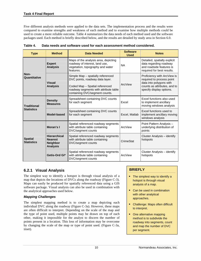
Five different analysis methods were applied to the data sets. The implementation process and the results were compared to examine strengths and weakness of each method and to examine how multiple methods could be used to create a more reliable outcome. Table 4 summarizes the data needs of each method used and the software packages used. Each method is briefly described below, and the results are detailed by study area in Section 6.0.

Table 4. Data needs and software used for each assessment method considered.

Type Method Data Needed Software

Used Notes

Expert Analysis

Maps of the analysis area, depicting roadway of interest, land use, vegetation, topography and water features.

NA

Detailed, spatially explicit data regarding roadway and roadside features is required for best results.

Non-Quantitative

Visual Analysis

Simple Map – spatially referenced DVC points, roadway data layer. Coded Map – Spatial referenced roadway segments with attribute table containing DVC/segment counts.

ArcView

Proficiency with ArcView is required to process point data into polygons with counts as attributes, and to specify display options.

Density Measures

Spreadsheet containing DVC counts for each segment Excel

Excel functions also used to implement ancillary moving windows analysis Traditional

Statistics

Model-based Spreadsheet containing DVC counts for each segment Excel, Matlab

Excel functions used to implement ancillary moving windows analysis

Moran’s I Spatial referenced roadway segments with attribute table containing DVC/segment counts

ArcView Point Pattern Analysis – underlying distribution of points

Hierarchical Nearest Neighbor Analysis

Spatial referenced roadway segments with attribute table containing DVC/segment counts

CrimeStat

Cluster Analysis – identify hotspots Spatial

Statistics

Getis-Ord Gi* Spatial referenced roadway segments with attribute table containing DVC/segment counts

ArcView Cluster Analysis – identify hotspots

BRIEFLY

The simplest way to identify a hotspot is through visual analysis of a map.

Can be used in combination with other analytical approaches.

Challenge: Maps often difficult to interpret.

One alternative mapping method is to subdivide the roadway into segments, count and map the number of DVC per segment.

6.2.1 Visual Analysis The simplest way to identify a hotspot is through visual analysis of a map that depicts the locations of DVCs along the roadway (Figure C-3). Maps can easily be produced for spatially referenced data using a GIS software package. Visual analysis can also be used in combination with the analytical approaches used below.

Mapping Challenges

The simplest mapping method is to create a map depicting each individual DVC along the roadway (Figure C-3a). However, these maps are often difficult to interpret. Depending on the scale of the map and the type of point used, multiple points may be drawn on top of each other, making it impossible for the analyst to discern the number of points present in a location. This loss of information may be overcome by changing the scale of the map or type of point used. (Figure C-3a, inset).


Task 4 Final Report

Mapping Alternatives

An alternative mapping method is to subdivide the roadway into segments, count the number of DVC per segment and create a map showing each segment labeled with the number of DVC in that segment (Figure C-3b). Mile-long segments are intuitive since most roads have mile markers. The ease of visual interpretation can be increased by color coding the segments to correspond a continuum of low, medium, and high DVC counts (Figure C-3c).

A segment or multiple segments were identified as a hotspot based on the context of the surrounding segment values, i.e.: “I know a hotspot when I see one.”

6.2.2 Density-Based Analysis DOTs have traditionally used density-based analyses to identify locations where crashes appear to be more common. After visual analysis, this type of analysis is the most common for identifying DVC hotspots. A variety of metrics can be used to compare the DVC occurrence between locations, including the average, minimum, maximum, or standard deviation of the density, rate, or frequency of collisions on the segment of interest. All these metrics require the study area to be segmented and number of DVC that occur in each segment to be counted.

BRIEFLY

The most common type of analysis to identify DVC hotspots after visual analysis.

Can use a variety of metrics.

Metrics require study area to be segmented and DVCs /segment counted. How it Works

A density-based analysis compares each segment’s DVC count to the mean number of DVC/segment across the study area. Potential thresholds to designate a segment as having an abnormally high density of DVCs include:

any segment with more than the average number of DVCs/mile,

segments that exceed the mean count by one, two, or three standard deviations, or

values above the 95% confidence interval (CI) to be significantly larger than the mean.

Figure C-4 illustrates how the number and location of the hotspots identified by each of these density-based thresholds may vary, using the I-35 study area as an example. For normally distributed data, values greater than the 95% CI or values greater than three standard deviations from the mean are most commonly used to define outliers. The 95% CI yielded identical results to the greater than the mean definition in this example, and was very liberal in identifying hotspots, while the latter threshold (three standard deviations from the mean ) was extremely strict, identifying only one segment as a hotspot in this example (and no hotspots at all in the remaining three study areas). The choice of threshold obviously will have a profound effect on the number and location of hotspots identified.

DEFINED

Mean: Obtained by adding several quantities together and dividing the sum by the number of quantities. Can be synonymous with “average.”

Standard Deviation: The average amount by which scores in a distribution differ from the mean. Defined as the square root of the variance.

Confidence Interval: A statistical measure of the likelihood that an experimental result is true and not the result of chance alone.

Lack of Normality and the 95% Confidence Interval

None of the data from the four study areas is normally distributed, a common occurrence with crash data. Because the interpretation of the outlier thresholds discussed above relies on an assumption of data normality, the reliability of using these methods to identify hotspots is questionable. However, as part of a comparative framework, this method was carried forward, using the 95% CI as the threshold value to identify hotspots. The 95% CI was chosen to as it is congruent with the threshold used in the model-based approach, providing a comparison with the results achieved when the true underlying distribution of the data is considered.


Task 4 Final Report

6.2.3 Modeling A definition of a hotspot is “a location where more DVCs occur than are expected by chance.” Using this definition requires constructing a model that estimates the expected number of DVC along a segment of road. A modeling approach used for many different types of questions is to first determine the underlying distribution of the data under consideration and then identify those values that exceed a chosen probability of occurrence, based on the curve of the distribution. This is the type of approach used in Empirical Bayes-based before/after analyses to determine the expected number of crashes along a highway segment undergoing safety improvements.

Making the Data Work

The data used for this study are considered static and therefore do not represent a before/after scenario, but the modeling approach used by the Empirical Bayes method to estimate the probability of DVC occurrence can still be employed. The Empirical Bayes method chooses between two distributions to describe the probability of an observed DVC/mile value.

If the mean DVC/mile > variance of DVC/mile for the road segment of interest, then a Poisson distribution should be used.

When the mean < variance, a negative binomial distribution is more appropriate.

The variance exceeded the mean in all four of the data sets considered for this project. The parameters for the negative binomial distribution were calculated for each data set in Matlab using the function nbinfit(). Although the data manipulations are simple, this method requires access to and familiarity with Matlab or similar software, and the user must correctly apply the parameters of the negative binomial function to determine the value of the chosen DVC/mile hotspot threshold.

For the purposes of this comparison, a conventional threshold, values with <5% probability of occurrence, was chosen and only a few, small hotspots were identified in each of the four study areas. In practice, a less strict threshold (e.g., <10% probability of occurrence) could be used, based on user preference and the goals of the analysis.

Moving Window Routine

Additionally, as a way of examining the influence of segment’s neighbors on hotspot identification, a moving windows routine was applied to the binomial model’s results using Excel. Figure C-5 illustrates how the size and location of identified hotspots varies between the unmanipulated <5% threshold and a three-mile moving window. The three-mile window considers a segment and its two immediate neighbors, and was carried forward for comparison with the spatial statics (see below) as an alternative approach to capturing the influence of each segment’s immediate neighbors.

DEFINED

Empirical Bayes Methods: A class of methods which use empirical data to evaluate / approximate the conditional probability distributions that arise from Bayes' theorem. These methods allow one to estimate quantities (probabilities, averages, etc.) about an individual member of a population by combining information from empirical measurements on the individual and on the entire population.

Poisson Distribution: A discrete probability distribution that expresses the probability of a number of events occurring in a fixed period of time if these events occur with a known average rate and independently of the time since the last event.

Binomial Distribution: A discrete probability distribution of the number of successes in a sequence of n independent yes/no experiments, each of which yields success with probability p.

The Poisson distribution resembles the binomial distribution if the probability of an event is very small.

DEFINED

Monte Carlo Simulation: A known or hypothetical population is sampled repeatedly, and the outcomes averaged to determine the average value. Monte Carlo methods are useful for modeling phenomena with significant uncertainty in inputs.

Monte Carlo Simulations

Note: Monte Carlo simulations could also be used to determine the expected number of DVC/ mile. As noted in Section 5.1.1, it is possible to script a routine in ArcView that will apply a given number of points randomly to a line, and then count the number of points that are assigned to each mile long segment. This script can then be used as the basis for a Monte Carlo simulation to determine an average number of DVC/mile. However, scripting skills are required, and running the


Task 4 Final Report

simulation may be time intensive, depending on the amount of computing power available. Even though the Bayesian-type modeling approach described above requires using ancillary software packages, it is overall a more straightforward approach.

6.2.4 Spatial Statistics Spatial statics were developed to explicitly address the relationship of features based on their distribution in space and the values associated with the features. Many different tests are available.

The ArcView and the CrimeStat software packages offer spatial statistic capabilities, and other packages are also available.

Arc View’s Getis-Ord Gi* statistic application and CrimeStat’s hierarchical nearest neighbor (HNN) technique were used to identify DVC clusters in the study area.

These two approaches use different data inputs (features with values vs. individual points) but both require the user to input a distance band which defines the search area used to identify clusters.

Getis-Ord Gi* Statistic

The Getis-Ord Gi* statistic examines the clustering of segments with many DVCs as compared to the clustering of segments with few DVCs. This approach looks at each feature in a data set within the context of neighboring features.

A feature with a high value is interesting, but may not be a statistically significant hotspot.

To be a significant, a feature will have a high (low) value and be surrounded by other features with high (low) values as well.

The local Gi* sum for a feature and its neighbors is compared proportionally to the sum of all features.

When the local sum is different (larger or smaller) than the expected local sum and that difference is calculated to be too large to be the result of random chance, that feature is designated as hotspot (or cold spot), depending on the magnitude of the difference.

ArcView acts as black box to undertake all the necessary calculations to identify hot and cold spots, calculate their statistical significance, and automatically displays the results graphically.

The Getis-Ord Gi* approach requires the user to input a distanced band to determine the size of the local neighborhood and hence the number of neighbors to consider. The results are somewhat sensitive to the size of radius chosen. A rule of thumb for this approach is to choose a distance band that includes eight neighbors, unless initial cluster analysis (e.g., Moran’s I) suggests clustering is pronounced at some other distance. Therefore, unless the result of the initial Moran’s I point pattern analysis test suggested another distance, a four mile radius was used to generate results to compare to the other methods under consideration.

Hierarchical Nearest Neighbor

The hierarchical nearest neighbor (HNN) approach tests for clustering by identifying groups of points that are spatially close based on user defined criteria. Point data, rather than segments with values, are required for this approach. The user specifies a search radius and minimum number of points needed to define a cluster, and these criteria are the used by the HNN routine to assign points to a cluster.

BRIEFLY

The Hierarchical Nearest Neighbor (HNN) form of clustering can be single-level or multi-level hierarchical (NNh) and is particularly applicable if the nearest neighbor distance is believed to influence the problem being considered.

The CrimeStat HNN routine takes a user-defined threshold distance and compares the threshold to the distances for all pairs of points.

Only points that are closer to one or more other points than the threshold distance are selected for clustering.

Only points that fit both criteria - closer than the threshold and belonging to a group having the minimum number of points, are defined as clustered at the first level (first-order clusters).


Task 4 Final Report

The routine then conducts subsequent clustering to produce a hierarchy of clusters.

• The first-order clusters are themselves clustered into second-order clusters. Again, only clusters that are spatially closer than a threshold distance (calculated anew for the second level) are included.

• The second-order clusters, in turn, are clustered into third-order clusters, and this re-clustering process is continued until either all clusters converge into a single cluster or, more likely, the clustering criteria fails (Levine 2010).

CrimeStat acts as black box to undertake all the necessary calculations to identify clusters that meet the input criteria and can store the results as a shapefile that can then be viewed using ArcView. Other viewing options are also available.

After hotspot locations have been identified, CrimeStat can determine the likelihood that the identified clusters were identified by chance. However, this simulation is based on the area of the minimum enclosing rectangle for the points under consideration and is therefore not appropriate for data distributed along a line (e.g., DVC on a road). Thus, for DVC data, this method has no statistical rigor and therefore is more appropriately considered another version of visual analysis. Like the maps suggested in Section 5.2.1 for visual analysis, the CrimeStat HNN graphical output can be inspected for location of the clusters identified, and the intensity of these clusters can be subjectively compared. The HNN method does not provide an objective basis for designating a hotspot. Instead, the users choice of minimum number of points to consider, search radius and professional judgment provide the basis to identify a hotspot.

The results are sensitive to both the user-input criteria, as illustrated in Figure C-6, and the CrimeStat documentation offers no theoretical basis for choosing these inputs. Instead, knowledge about the system being examined should guide the choice input.

Because a one-mile long segment was used as the basic unit of comparison for other approaches, a radius that would consider a comparable-sized area was chosen (radius = 0.5 mile).

The number of points considered for each study area was defined as the mean number of DVC/segment + 1 standard deviation for that study area.

6.2.5 Expert Opinion To identify DVC hotspots using expert analysis, collision data are not considered. Instead, deer biologists (experts) familiar with the characteristics of the landscape and roadway in the study area identify the locations where they believe deer are most likely to cross the road.

For this analysis, detailed information about the roadway characteristics was not available. Roadway characteristics such as variations in lanes/roadway width and location of barriers (e.g., guardrail, Jersey barrier, steep embankments) are known to influence crossing locations (Barnum 2003). Additionally, the information about the characteristics (vegetation, topography) of the surrounding habitat, also known to influence crossing locations (Barnum 2003), was relatively coarse.

Because of this lack of detailed data, only the Iowa study areas (Figure C-7) were considered as both the roadways and the surrounding landscape was perceived to have little variation and to be relatively well-described by the available data, as compared to the New York study areas. Three biologists undertook the analysis, working separately.

Segments designated as a crossing zone by two analysts were coded as a warm spot.

Segments designated as a crossing zone by all three analysts were coded as hotspots.

The results of expert opinion analysis compared favorably with the actual DVC data, and the other methods for both Iowa study areas.

In both study areas, all but one segment identified as warm/hot either overlapped with or was adjacent to segments with a higher than average number of actual DVCs.


Task 4 Final Report

The hotspots were located either in or adjacent to hotspot areas identified by the bulk of the other methods.

It should be noted that the biologists who undertook this exercise were not deer biology experts. It is likely that deer experts familiar with the biology of local herds and with true knowledge of local roadways and landscape would perform better.

7.0 RESULTS

All the methodologies discuss above were applied to all four study areas.

Additionally, a moving window routine using a three-mile window was applied the binomial model results.

The results of each method were mapped using ArcView, and are presented side-by side in the figure for each study area (Figures A-8 through A-11) for the reader to compare visually.

The number of segments identified as hot by each method, as well as the overlap among methods is summarized for each study area in Tables 4 and 5.

Table 5. Number and proportion of segments identified as hotspots by each method.

I-35 Route 65 I-90 Route 28

Method Count Proportion Count Proportion Count Proportion Count Proportion

Average 23 0.48 15 0.29 13 0.26 20 0.40

Binomial 5 0.10 3 0.06 7 0.14 5 0.10

3-Mile Window 2 0.04 4 0.08 0 0 0 0

Getis-Ord 2 0.04 7 0.14 12 0.24 17 0.34

HNN 8 na* 4 na* 8 na* 7 na*

Expert 11 0.23 11 0.22 na na

*The location of the hotspots identified by the HNN approach does not correspond to the segments used in by the other approaches, and therefore the proportion is not comparable.

Table 6. Overlap of segments identified as hotspots.

Overlap* I-35 Route 65 I-90 Route 28

Segments identified as hot by at least two methods

Segments 4, 6, 9, 34, 39, 41, and 45

Segments 12, 17, 18, 19, 20, 32, and 46-48

Segments 10, 20, 21, 35, 38, 39, 43, and

49

Segments 4-6, 15, and 16

Segments identified as hot by at least three methods

Segments 6, 34, 39 Segments 46 - 48 Segments 43, 49 Segments 4-

6, 15, 16

Segments identified as hot by all methods

None Segment 47 None None

*The location of the hotspots identified by the HNN approach does not correspond to the segments used in by the other approaches, and therefore this method is not included in this comparison.


Task 4 Final Report

7.1 IOWA I-35

The I-35 study area was 48 miles long, runs north-south and contained the most DVCs of the four study areas (287). The segments identified as hotspots by the six cluster analysis methods applied are depicted for comparison in Figure C-7, summarized in Table 4 and 5, and results are briefly summarized below.

BRIEFLY

48 miles long, runs north-south

Contained the most DVCs of the four study areas

Moran’s I results suggest that DVC are randomly distributed, rather than clustered

See Figure C-8

Point Pattern Analysis: The initial Moran’s I test for intensity of clustering of segments with high or low values indicated no clustering at any of the distance bands tested. This result suggests that the DVC along I-35 are randomly distributed. Despite this finding, the cluster analyses were conducted on these data for comparative purposes.

Visual Analysis: Based on the raw DVC/mile counts and the color coding scheme used on the map that depicts the raw counts, an area of high-count segments appears to be located from segments 3 through 9 and 49 through 41. However, this pattern appears weak, as high count segments are distributed throughout the study fairly evenly.

Density Based Comparison: The average number of DVC/mile for I-35 was 5.98, and the upper 95% CI cut-off is 6.96. Using this liberal definition of a hotspot, nearly half (23 of 51) of the segments were identified as a hotspot. This was the greatest number and proportion of segments to be identified as hotspots in any of the study areas (Table 4).

Binomial Model: The calculated hotspot threshold based on the binomial distribution for the I-35 data was 11 DVC/mile. Using this cutoff, five segments were identified as hotspots (4, 9, 35, 39, and 41).

Spatial Statistics: Because the initial Moran’s I test for clustering failed at all distance bands tested, there was no objective reason to chose any particular distance band for the Getis-Ord test. Based on the recommendation that at least eight neighbors should be considered by the test, the four-mile distance band was chosen for the analysis. Using the four-mile search radius, only a single, small weak hot spot (segments 6-7) was identified, and it is interesting to note that no hotspots were identified at the eight- and twelve-mile distance bands. This result suggests that although there are some segments with higher DVC/mile values, they are not exceptionally high relative to all other segments included in the analysis.

The HNN technique identified eight hotspots that corresponded generally to hotspot areas identified by the density-based analysis. The HNN graphical output provided a relatively concise hotspot pattern as compared to the visual and the density based analyses.

SUMMARY

Overall, the results of the cluster analysis are congruent with the initial Moran’s I finding of a random distribution of high and low value segments. A consistent pattern of hotspot distribution was not apparent across the seven methods compared.

Expert Analysis: The expert analysis identified 11 segments as warm or hot. The two segments identified as hot, 6 and 35, coincide with segments identified by Getis-Ord and the binomial model as hot, respectively. All but one segment identified as warm/hot either overlapped or with or were adjacent to segments with a higher than average number of actual DVCs (Figure C-7).The features that experts identified as attractive to deer do indeed appear to be associated with DVCs.


Task 4 Final Report

7.2 IOWA ROUTE 65

BRIEFLY

51 miles long, runs north south

Moran’s I results suggest strong clustering

See Figure C-9

The Route 65 study area was 51 miles long and runs north-south. The segments identified as hotspots by the six cluster analysis methods applied are depicted for comparison in Figure C-8 and summarized in Table 4 and 5, and results are briefly discussed below.

Point Pattern Analysis: The initial Moran’s I test for intensity of clustering of segments with high or low values indicated strong clustering at the two, four, and eight-mile distance bands. This result suggests that the DVC along Route 65 are not randomly distributed. Visual Analysis: Based on the raw DVC/mile counts and the color coding scheme used to the map that depicts the raw counts, there appear to be two hotspots in the Route 65 study area, consisting of segments 17 -22, and segments 46-49, respectively.

Density Based Comparison: The average number of DVC/mile for Route 65 was 4.94, and the upper 95% CI cut-off is 6.31. Using this liberal definition of a hotspot, 15 of the 51 segments were identified as a hotspot, including two hotspots four segments in length that corresponded with the hotspots from the visual analysis (segments 17-20, and segments 46-49).

SUMMARY

The results from all the cluster analysis methods for this study area were congruent, identifying a large, strong hotspot at the northern end of the study area, and either identifying or suggesting a weaker, less focused hotspot between segments 12 and 20. This is not surprising, as the DVC value for segment 47 is so much larger then the next nearest value (27 vs. 13) there is no question that it should be regarded as a hotspot, and the study area’s second highest DVC/segment value (16) is occurs in segment 18. These imbalances are immediately apparent upon visual inspection of the maps, and they drive results of all the mathematically based analyses as well.

Binomial Model: The calculated hotspot threshold based on the binomial distribution for the Route 65 data was 13 DVC/mile. Using this cutoff, three segments were identified as hotspots (17, 46, and 47). Under the 3-mile window moving windows scenario, the hotspot at segment 17 dropped out, but the hotspot at segments 46/47 expanded to include the segments from 46 through 49. These results correspond closely with both the visual analysis and the density-based comparison results.

Spatial Statistics: The Getis-Ord test identified a large, intense hotspot in the Route 65 study area from segment 45-50, and a small, weak hot spot consisting of segment 19. This result is consistent with the results from the other cluster analysis methods.

The HNN technique identified four hotspots that corresponded generally to hotspot areas identified by the density-based analysis and the expert analysis.

Expert Analysis: The expert analysis identified four segments as warm and seven as hot. Two of the segments identified as hot, 47 and 48, were also identified as hot by all other methods, while segment 17 was identified as hot by all other methods except the Getis-ord test and moving windows. All but one segment identified as warm/hot either overlapped or with or were adjacent to segments with a higher than average number of actual DVCs. The features that experts identified as attractive to deer do indeed appear to be associated with DVCs.


Task 4 Final Report

7.3 NEW YORK I-90

The I-90 study area is 50 miles long and runs east-west. The segments identified as hotspots by the six cluster analysis methods applied are depicted for comparison in Figure C-9, and summarized in Table 4 and 5, and results are briefly discussed below.

BRIEFLY

50 miles long, runs east-west

Moran’s I results suggest clustering at larger scales

See Figure C-10

Point Pattern Analysis: The initial Moran’s I test for intensity of clustering of segments with high or low values indicated a sharp increase in clustering at the eight-mile distance band. This result suggests that the DVC along I-90 are not randomly distributed, particularly at larger scales.

Visual Analysis: Based on the raw DVC/mile counts and the color coding scheme used on the map that depicts the raw counts, there appears to be a discrete hotspot at segments 20-21, and a cluster of higher value segments at the western end (segments 35-50) of the study area. However, the pattern of higher and lower value segments is mixed in this section, and does not clearly suggest that the entire section should be designated a hotspot or that only certain segments should be designated as hotspots. This portion of I-90 provided a good illustration of the limitations of visual analysis.

Density Based Comparison: The average number of DVC/mile for I-90 was 4.36, and the upper 95% CI cut-off is 5.01. Using this liberal definition of a hotspot, 13 of the 50 segments were identified as a hotspot. The pattern was very similar to the visual analysis, including segments 20 and 21, and similar mix of hot/not hot segments in the western end of the study area.

SUMMARY

Visual analysis, the density based comparison, the Getis-Ord test, and the HNN technique identify or strongly suggest the entire western as an extended hotspot. All approaches except the moving windows technique identify segments 20-21 as a hotspot, while the Getis-Ord test identified a cool spot at segment 19. This may suggest a focused area of crossing by deer in the 20-21 segments, potentially facilitated by specific habitat feature, such as an area that provides an exceptional food or shelter resource.

Binomial Model: The calculated hotspot threshold based on the binomial distribution for the I-90 data was 8 DVC/mile. Using this cutoff, seven segments were identified as hotspots (10, 20-21, 35, 38, 43, and 49). Under the 3-mile window moving windows scenario, no hotspots were identified.

Spatial Statistics: The Getis-Ord test identified a single, large hotspot area in western part of the I-90 study area, segments 39 - 50. The test also indentifies a large cool spot at segments 7-11.

The HNN technique identified eight hotspots that corresponded generally to hotspot areas identified by the density-based analysis and the model-based analysis.


Task 4 Final Report

7.4 NEW YORK ROUTE 28

The Route 28 study area is 50 miles long and runs roughly northeast-southwest. The segments identified as hotspots by the six cluster analysis methods applied are depicted for comparison in Figure C-10 and summarized in Table 4 and 5, and results are briefly discussed below.

BRIEFLY

50 miles long, runs NE- SW, and has a hilly topography

Moran’s I results suggest clustering

See Figure C-11

Point Pattern Analysis: The initial Moran’s I test for intensity of clustering of segments with high or low values indicated significant clustering at all distance bands. This result suggests that the DVC along Route 28 are not randomly distributed.

Visual Analysis: Based on the raw DVC/mile counts and the color coding scheme used on the map that depicts the raw counts, there appear to be distinct hotspots at segments 1, 6, 15-17, and 26-28.

Density Based Comparison: The average number of DVC/mile for Route 28 was 2.44, and the upper 95% CI cut-off is 2.96. Using this liberal definition of a hotspot, 20 of the 50 segments were identified as a hotspot. The pattern was similar to the visual analysis, and included all the segments identified as hotspots through that approach.

Binomial Model: The calculated hotspot threshold based on the binomial distribution for the Route 28 data was 5 DVC/mile. Using this cutoff, five segments were identified as hotspots (4, 6, 15-16). Under the 3-mile window moving windows scenario, no hotspots were identified.

Spatial Statistics: A 12-mile distance band was used for the Getis-Ord test, as this distance band generated the largest Z in the Moran’s I test (Z = 5.23, p = 0.01) The Getis-Ord test identified a large, contiguous warm to hotspot in the western end of the study area that encompasses segments 3-18, with the greatest intensity occurring from 14-18. The test also indentifies a large cool spot at segments 33-50.

SUMMARY

Visual analysis, the density based comparison, and the Getis-Ord tests identify or strongly suggest the entire western as an extended hotspot. The binomial model is more conservative, but the hotspots that it identifies are also in the western part of the study area.

The HNN technique identified seven hotspots that corresponded generally to hotspot areas identified by the density-based analysis. The HNN graphical output provided a relatively concise hotspot pattern as compared to the visual and the density based analyses.


Task 4 Final Report

8.0 COMPARISON OF METHODS

8.1 UNDERLYING DISTRIBUTION

We recommend beginning any analysis by determining if the underlying distribution of DVCs across the study area is random, even, or clustered. Although visual inspection of mapped DVCs can give some indication of the type of distribution, patterns that appear random may indeed be clustered at certain scales. Using a test like Moran’s I will identify if clustering is present, at what scale it is present, and provide a valuable guide as to if further analysis is warranted. As discussed in section 5.1.1, another approach to testing the underlying distribution of DVC data is to use a Monte Carlo to determine the hypothetical average nearest neighbor distance for the DVC in the sample for comparison to the actual average. Both approaches provided meaningful results, and Moran’s I has the advantage of off–the-shelf availability in a variety of software packages (including ArcView).

8.2 HOTSPOT METHODS

In general, visual analysis is useful as a starting point for identifying hotspots.

For some simple, clear-cut patterns, like those seen in the Route 65 study area, visual analysis my be sufficient. conducting additional quantitatively-based analyses may add only a limited amount of new information, and serve instead to confirm the initial impression.

For less clear cut patterns, like the other three study areas, additional mathematically-based analyses can bring greater confidence to the initial, visual impression of the location of significant DVC hotspots.

Advantages of visual analysis are its intuitive appeal and straightforward implementation. Disadvantages include a lack of clear-cut, objectively defined rules to identify hotspots.

Density-based measures that rely on an assumption of underlying data normality appear to be the least useful type of quantitative analysis, as crash data are generally not normal. While straight forward to implement with basic spreadsheet function and intuitively appealing, applying commonly-accepted thresholds to identify outliers appears ineffective. The 95% CI (incorrectly calculated on an assumption of normality) yielded results that appear substantially similar to visual analysis, while three standard deviations from the mean appeared to be overly strict. Because other quantitative methods do offer mathematically correct, objective methods to chose a threshold, density measures do not appear offer much value, except used as a stand-in for visual analysis.

BRIEFLY

Visual Analysis: Useful starting point

Density-Based Measures: Generally mathematically inappropriate.

Model-Based Analysis: Mathematically appropriate but may be complex to implement

Spatial Analysis Methods: Specifically designed to examine spatial relationships, such as clustering. Software packages widely available, but are generally developed for points distributed across an area, rather than along a line. User-specified criteria inserts an element of subjectivity.

Expert Opinion: Hotspots identified had good overlap with high DVC segments. May be particularly useful when a relatively extensive area has been identified as a hotspot, and a specific location within that area will be chosen for placement of an under- or overpass.

Model-based analysis has the advantage of being appropriate for non-normal data and generating an objective hotspot threshold. Disadvantages of this approach are that it is moderately complex to implement, and that the results at 95% probability of occurrence seem somewhat strict. However, as noted in Section 5.2.3, a more relaxed probability of occurrence (e.g., 90%) can be adopted if desired.

Spatial analysis methods such as average nearest neighbor, Getis-Ord, and HNN were specifically designed to examine spatial relationships, such as clustering, in an objective manner.


Task 4 Final Report

Software packages that offer spatial analysis options are widely available, a variety of analyses exist, and more are likely to be created as the relatively young field of spatial statistics continues to mature.

An advantage of these methods is that spatial analysis software packages include routines that calculate the statistical significance of the spatial patterns that they identify.

However, users must be aware that spatial analysis methods are generally developed for points distributed across an area, rather than along a line. The statistical significance tests used by some methods (e.g., nearest neighbor analyses) must be adapted to provide accurate results for spatially linear data. Although these adaptations may not be available of-the-shelf, they can readily be implemented by using the programming options offered by many software packages that offer spatial analysis capabilities.

As noted above, spatial analysis approaches have been designed to analyze spatial relationships using objective, quantitative methods. However, users must specify the criteria (e.g., study area size, search radius, number of points to consider, etc) that guide the quantitative analyses, and must be aware that the results are sensitive to the choice of these input parameters, to varying degrees. Choosing the values of these criteria is always a subjective process that requires knowledge of the system under study. For some approaches, subjectivity can be lessened by using ancillary tests.

Expert opinion appears to offer some value to the hotspot identification process. Even for this analysis, which relied on biologists who were not deer experts per se and who did not have access to the best data, the hotspots identified had good overlap with high DVC segments. The features that experts identified as attractive to deer do indeed appear to be associated with DVCs. Expert opinion may be particularly useful when a relatively extensive area has been identified as a hotspot, and a specific location within that area will be chosen for placement of an under- or overpass. Because of the expense of these structures, every effort should be made to place them in the most effective locations.

Table 7 provides a summary comparison of strengths and weaknesses of the five methods tested.


Task 4 Final Report

Table 7. Comparison of analysis methods assessed under Task 4.

Type Method Strengths Weaknesses

Expert Analysis

Conducted by a group of experts.

No DVC data required Sufficiently detail data may be lacking, especially about roadway features

Simple Map – plot all locations.

Intuitively appealing and maps are easily produced with GIS

Data loss and lack of objective thresholds to define a hotspots

Non-Quantitative

Visual Analysis Coded Map – code

segments to indicate locations with multiple DVC recorded.

Intuitively appealing; does require some expertise with GIS to create these maps

Difficult to create/apply objective criteria to define a hotspot

Density Measures

Average DVC/mile Intuitively appealing and easily calculated using standard spreadsheets

Most DVC data is non-normal; no inherent objective criteria to interpret resulting maps Traditional

Statistics

Model-based

Expected DVC/mile estimated from the binomial frequency

Appropriate for non-normal data; uses expected number of DVCs as a hotspot threshold.

Somewhat complex to implement; results may be conservative

Average Nearest Neighbor Distance (NND)

Intuitively appealing Off-the-shelf software unsuitable for linear NND applications

Point Pattern Analysis Moran’s I (ArcView) Output easily interpreted Black box functionality,

user defined inputs

Hierarchical Nearest Neighbor (HNN) Analysis (Crimestat)

Spatial analyses are designed specifically to identify cluster location.

Black box functionality; user defined inputs; off-the-shelf significance tests unsuitable for linear HNN applications

Spatial Statistics

Cluster Analysis

Getis-Ord Gi* (ArcView) Spatial statistics are designed specifically to analyze cluster location, and intensity.

Black box functionality; user defined inputs


Task 4 Final Report

8.3 CHOOSING A METHOD

The results of this comparison of methods do not suggest a basis for choosing a single “best” method to identify DVC hotspots. Model-based and spatial statistic methods do allow objectively based criteria to be applied, yielding greater confidence in the results. However, all methods require user in puts (e.g., size of study area, segment size, significance level, etc), and the value of these inputs must be justified based on familiarity with the area under study and the goals of the analysis.

In some cases the system under study may not provided any good theoretical basis for choosing the value of these inputs. Additionally, for the more quantitative approaches, the analyst must bear in mind that statistical significance may not equal biological significance.

Model-Based Approaches and Spatial Statistics

We recommend using model-based approaches and spatial statistics because they reduce subjectivity of interpretation to some degree. We also recommend applying multiple approaches, comparing the outcomes visually, (e.g., Figures A-8 through A-11) and looking for the locations that are repeatedly identified as a hotspot. This may consist of comparing two or more different approaches. Alternatively, the inputs of a single approach can be varied and compared. For example, the value of a CI for model-based approaches or the search radius of the Getis Ord test can be varied. Visually comparing these quantitative results to segmented visual analysis map or the clusters identified by HNN provides a useful “reality check” to the underlying data.

BRIEFLY

Use model-based approaches and spatial statistics because they reduce subjectivity of interpretation to some degree.

Apply multiple approaches, comparing the outcomes visually, and looking for the locations that are repeatedly identified as a hotspot.

Consider the goal of the analysis when choosing one the approach(es) to identify a hotpot.

Consider the Goal of the Analysis

We also recommend considering the goal of the analysis when choosing one the approach(es) to identify a hotpot. As an example of choosing a method that fits the goal of the analysis, consider that there are two main approaches to mitigating DVC known to be effective: fencing, and underpasses.

Fencing must be extensive to be effective. Methods that are not conservative (visual analysis, Getis-ord) and that work well over large areas may be best to identify longer highway segments that are good candidates for fencing.

Underpasses require a high degree of specificity, and a model-based approach with strict threshold may be the best approach to identify specific DVC hotspots. However, topography and roadway design heavily influence where an underpass can be placed, and the specific locations identified as DVC hotpots may not lend themselves to underpass construction. Using a less conservative method and then focusing in on the exact underpass locations in consultations with the road designers and a deer expert may be the best approach.


Task 4 Final Report

9.0 PREDICTING DVC LOCATIONS

Any approach used to identify the factors associated with existing DVC locations can also potentially be used to predict new DVC locations, either in response to changes in land use in the landscape around a roadway or, on planned and/or newly constructed roadway segments. All of the methods discussed in Section 6.2 could be used in this predictive fashion, as well as the additional approaches identified in the literature review. However, only two predictive applications were identified in the literature reviewed (discussed blow) and no predictive applications were identified in the DOT interviews.

In order to predict DVC locations (the dependent variable), at least one independent variable is required. Independent variables may come from the roadway (e.g., posted speed limit, traffic volume, number of lanes, location of bridges), roadside (e.g., location of guard rails, cuts, fills), and/or landscape (e.g., cover type, cover type heterogeneity, land uses, topography). The research reviewed in the literature review considered a myriad of factors that are known to influence habitat use by deer as well as factors known to influence collision rates. Broadly, these factors described to land use, habitat quality, topography, the roadway, and traffic. Table 2 in Appendix A summarizes variables determined to have a significant relationship with DVCs. Variables related either directly or indirectly to habitat quality were most likely to demonstrate trends. These variables indicate land uses incompatibly with deer habitat, or they describe the presence of forest/open habitat edges, which is the habitat type preferred by deer. Traffic speed and volume also clearly demonstrate an effect on the DVC rate. The relationship of topography and roadway geometry was less clear (Appendix A).

VARIABLES RELATED TO DVC

Land use

Habitat quality

Topography

The roadway

Traffic Two applications identified in the literature review were presented by the authors explicitly as predictive tools.

Expert Analysis Models

Hurly et al. (2009) present a formalized approach to developing an expert-based hotspot prediction model. For this type of model, one or more experts familiar with the biology of the species of interest are asked to identify the roadway and landscape variables that they feel are most likely to be associated with collisions. Locations along the roadway that most resemble the expert-described hotspots are then identified. Hurly et al. (2009) solicited and collected input from a group of experts, and then used GIS to combine the input and map the hotspot locations. They tested their approach using input from 10 moose experts to create a moose-vehicle collision (MVC) hotspot model, and determined the expert-based model to be in good agreement with known MVC locations. Based on these results, expert-based models appear to have utility in either identifying existing hotspots or predicting where new hotspots may occur. However, this approach depends on finding knowledgeable experts willing to participate in the process and also requires computational and software expertise to produce the expert-based model, making this approach at least as resource intensive as data-driven approaches.

STATISTICAL DISTANCE MODEL

Divides the roadway and surrounding landscape into cells.

Assign values based on spatial data attributes

Calculates the similarity distance of all mapped cells

Similarity distance of cell containing an event (e.g., a DVC) can be compared to all other cells; cells with small distances are potential event locations

Statistical Distance Models

A promising approach which relies on data from the landscape surrounding the roadway as well characteristics of the roadway is presented by Kolowoski and Nielsen (2008). Their approach uses a GIS-based statistical distance model to predict collision locations, using a data set of known bobcat roadkill locations. A GIS is used to divide the roadway and the surrounding landscape into cells, and assign values based on spatial data attributes (e.g., mean patch area, percent slope, traffic volume, number of houses, etc.) to each cell, and then calculates the similarity distance of all mapped cells to cells known to contain a bobcat roadkill. The similarity distance is calculated on the basis of the


Task 4 Final Report

similarity of spatial data attribute values between mapped cells. The cell size is user defined, based on the resolution of the available spatial data, as are the attributes considered for similarity measurements. A confidence interval of the expected similarity between cells can be constructed using a Monte Carlo simulation, and cells were similarity to the known roadkill locations exceed the upper bound of the chosen confidence interval are identified, designated as potential hotspots, and displayed graphically. Because spatial data that describes landscape attribute known to be related to DVC (Appendix A) is widely available, this approach can readily be implemented. It should be noted that the resolution of the data will dictate the resolution of the results, and although data is available, it may require manipulations before it can be used for this application.

10.0 CONCLUSION AND RECOMMENDATIONS

The literature examining DVC from an ecological perspective is reasonably well developed. Conversely, literature examining DVC from a safety perspective is sparse. The ecologically-based DVC literature provides a baseline from which to identify the factors most likely to be related to DVC locations, and which could reasonably be used to predict DVC locations when new roads are built, or when land use surrounding existing roads changes. However, theoretical examples of predictive applications are few, and no examples of real world use were identified. The use of predictive models is an area of DVC analysis that appears ripe for development.

A variety of approaches that can effectively identify DVC hotspots are available. The software and computing tools needed to implement these approaches are also widely available, including mapping tools that can effectively display the results for ease of interpretation. However, there is no objective basis for choosing a single best approach for DVC hotspot identification. The goal of the analysis influences which approach is most appropriate, and all methods are to a lesser or greater degree dependent on the user’s choice of study area extent and definition of a hotspot. Therefore, we recommend using multiple tests to identify hotspot locations and then compare results. Locations that are identified as hotspots by multiple methods or under varying criteria using a single method are likely to be the most significant hotspots in the area of study. Additionally, local knowledge of the system under study is required to make good decisions about which hot spots should be prioritized for countermeasures. There is no substitute for critical thinking when conducting these types of analyses.

IN SUMMARY

The knowledge and the tools to create predictive DVC models exist, but they have not yet been implemented

A variety of tools are available to identify DVC hotspots, and we recommend using and comparing the output of multiple methods

DVC hotspot identification should be more widely incorporated into roadway planning and design

While some states currently consider DVC hotspot locations as part of their roadway planning and design practice, and others are taking steps to improve their capabilities, DVC hotspot considerations are not universal. Because appropriate methods and tools to identify DVC hotspots are widely available and yield useful results, we recommend that DVC considerations be more widely incorporated into State’s roadway project planning and design, where DVC are indentified as a safety concern.


Task 4 Final Report


11.0 REFERENCES

Baily, T. C., Gatrell, A. C. 1995. Interactive Spatial Analysis. Pearson Education Limited. Essex, England. 413 pp.

Barnum, S. 2003. US Using Information About Wildlife Crossing Zones to Reduce Wildlife/Highway Conflicts. Doctoral Dissertation, University of Colorado at Denver. 142 pp.

Clevenger, A. P., Hardy, A., Gunson, K. 2008. Chapter 3.3 Hotspot Modeling in Evaluation of the Use and Effectiveness of Wildlife Crossings. NCHRP Report 615. Transportation Research Board.

Fotheringham, A. S., Brunsdon, C., Charlton, M. 2000. Quantitative Geography: Perspectives on Spatial Data Analysis. Sage Publications. London, England. 270 pp.

Ned Levine (2010). CrimeStat: A Spatial Statistics Program for the Analysis of Crime Incident Locations (v 3.3). Ned Levine & Associates, Houston, TX, and the National Institute of Justice, Washington, DC. July.

Task 4 Final Report

APPENDIX A – LITERATURE REVIEW

A-1 Normandeau Associates, Inc.

Literature Review


Task 2: Literature Review – Final Investigation of Methods to Identify and Prioritize

Deer-Vehicle Crash locations

February 2010

Literature Review

TABLE OF CONTENTS

1.0 Introduction........................................................................................................................... A-5

2.0 Identifying DVC Hotspots .................................................................................................... A-5

2.1 Non-Quantitative Methods................................................................................................... A-6

2.3 Traditional Statistics ............................................................................................................ A-8

2.3 Spatial Statistics................................................................................................................... A-9

3.0 Methods to Examine the relationship of DVCs to roadway and Environmental Factors......................................................................................................... A-9

4.0 Factors Associated with DVC Hot Spots.......................................................................... A-10

5.0 Predicting DVC Locations ................................................................................................. A-10

6.0 Sources of Data for DVC Analysis .................................................................................... A-10

7.0 Literature Cited ................................................................................................................... A-15

APPENDIX A:........CITED REFERENCES SUMMARIZED IN TABULAR FORMAT BY TOPIC AREA


Literature Review


LIST OF TABLES

Table 1. DVC hotspot identification methods.......................................................................................... A-7

Table 2. Variables determined to have a significant relationship with DVC locations, based on a review of 16 studies.*.............................................................................................................. A-11

Table 3. Data needed and generally available data sources for DVC hotspot identification and prediction................................................................................................................................. A-14

Appendix Table A1. Summary of cited hotspot methodology references............................................ A-18

Appendix Table A2. Summary of cited DVC/environmental factors methodology references............ A-20

Literature Review

1.0 INTRODUCTION

The following literature review provides an overview of: 1) the methods that can be used to identify deer-vehicle collisions (DVC) hotspots; 2) the variables that are associated with DVC hotspots; and 3) methods to predict likely DVC hotspots, based on their association with these variables. Additionally, sources of data to conduct DVC analyses are briefly reviewed. This review is an interim product that will provide background to the Final Report. The literature search focused on NCHRP publications to provide background on standard highway safety practices and peer-reviewed ecological journals to provide background on the study of deer–highway interactions. However, some grey literature reports were also available through various sources, and are included as well. Additional gray literature reports may be provided by DOT’s contacted for Task 3, and will be integrated into the final report, as appropriate.

There is a wealth of additional materials from the ecological literature that can also inform the study of DVCs. These unreviewed topics included moose-vehicle collision studies, general wildlife-vehicle collision studies, studies of how wildlife use habitat surrounding roads and investigations of where animals cross roads. Future investigations of DVC issues may gain additional insight by including these types of studies for consideration.

2.0 IDENTIFYING DVC HOTSPOTS

DVC hotspots can be indentified using any of the standard methods that safety personnel use to identify locations where an excessive number of all types of crashes occur over time. Additionally, ecologists studying the interactions of deer with highways have employed a variety of methods to identify DVC hotspots, some of which are the same or similar as those used by safety personnel, and some of which may be novel.

Department of Transportation (DOT) safety personnel have traditionally used density measures, often in combination with a sliding windows approach to identify crash hotspots. Persuad (2001) argues that much of the error that density measures are prone to, due to the inherent variability of crash data, can be overcome with the use of statistically-based modeling approaches. The new SafetyAnalyst tool (2009) developed by the FHWA uses a modeling approach to identify collision hotspots, and the use of this approach may therefore be poised to become more wide-spread among DOTs. To date, researchers interested in exploring the relationship of DVC hotspot locations to variables from the surrounding landscape and roadways have not generally used statistically rigorous approaches to identify hotspots either. In six of the studies reviewed (Appendix A, Table 1), the authors did not explicitly discuss the methods used to identify a hotspot, but they appear to have used some type of density measure. One study used a density measures-sliding windows approach (Singleton and Lehmkuhl 2000), one study used a formalized expert analysis (Hurley et al. 2009), and one study (Malo et al. 2004) used a modeling approach based on a statistical distribution. Additionally, DVC researchers have recently begun exploring and employing spatial statistics to identify hotspots (Clevenger et al 2008, Moutrhankis and Gunson, 2009).

All of the methods identified in this literature review are summarized in Table 1, and briefly discussed in the following text. The table includes a brief summary of each method, data needs, and its strengths and weaknesses. It is important to note that regardless of the method used, the results of all hotspot analyses are influenced by the measurement error as well as the temporal and spatial scale of the data used. No method can completely remove the limitations and biases inherent to the data set under consideration. The practitioner must apply some measure of professional judgment to ensure that the most appropriate data are used to answer the question being asked, and that the limitations of the results are understood by those who will use the results for decision making. Additionally, hotspot analysis requires a unit of comparison, i.e., a DVC hotspot only exists relative to some other location that has fewer DVCs. Although some methods may offer some theoretical guidance as to the appropriate length of the analysis unit along the roadway, this is another variable that must be chosen to some degree on the basis of professional judgment.


Literature Review


2.1 NON-QUANTITATIVE METHODS

Expert Opinion––Instead of looking at collision data, one or more experts familiar with the biology of deer are asked to identify the roadway and landscape variables that they feel are most likely to be associated with DVCs. Locations along the roadway that most resemble the expert-described hotspots are then identified. Hurly et al. (2009) present a formalized approach for soliciting and collecting input from a group of experts, and then used GIS to combine the input and map the hotspot locations. They tested their approach using input from 10 moose experts to create a moose-vehicle collision (MVC) hotspot model, and determined the expert-based model to be in good agreement with known MVC locations. Based on these results, expert-based models appear to have utility, and may be the only choice if collision data is unavailable. However, this approach depends on finding knowledgeable experts willing to participate in the process and computational and software expertise is required to produce the expert-based model, making this approach at least as resource intensive as data-driven approaches.

Visual Analysis––This approach simply requires plotting DVCs on a map of the road system under consideration and locations that appear to have a large number of DVC per unit distance are then identified visually. Visual analysis is intuitive and simple to implement, especially with the advent of GIS. However, the scale and type of display will have a substantial influence on the perceived location and size of hotspots, and the choice of display scale must be keyed to the density and distribution of the data under consideration to achieve reasonably accurate results. GIS platforms allow the user to change all these attributes with ease, and apply professional judgment to identify the best representation of the data under consideration. Locations with multiple DVCs will be obscured unless points are coded to represent multiple points. Using hollow, as opposed to filled, points to designate DVC locations is another approach for the observer to better perceive locations where points are stacked. Visual analysis can also be combined with density measures or modeling (see below) to produce maps of roadways coded to represent the chosen measures of comparison.

Literature Review

Table 1. DVC hotspot identification methods

Method Approach Description Data Needs Primary Strengths and Weaknesses

Expert Analysis

Conducted by a single expert or a group of experts

Characteristics of the landscape and habitat surrounding the roadway

Roadway characteristics

Can be used when no DVC data is available Only as good as the experts used

Simple Map – plot all locations DVC locations represented by a distance measurement or x, y coordinates

Easily implemented and intuitively understood Important information is obscured Results heavily dependent on scale of display

Non-Quantitative

Visual Analysis

Coded Map – code points to indicate locations with multiple DVC recorded

DVC locations represented by a distance measurement or x,y coordinates

Easily implemented and intuitively understood Codes can be based on simple counts, density measures, or model- based analysis

Results dependent on scale of display

Density Measures

Calculate the average (or min, max, standard deviation, etc) number, rate or frequency of collisions on the segment of interest, then identify locations where the chosen value of comparison is exceeded.

DVC counts for each segment of interest

Easily implemented and intuitively understood Results may be used alone or combined with ranking methods

Inherent variability of crash data can lead to errorsNo objective estimate of expected collision frequency

Traditional Statistics

Model-based Determine the expected number of DVCs along a segment using a model and compare the observed to the expected number to determine if the section is a hot spot

DVC counts for each segment of interest

Safety Performance Function (SPF) for some applications

Objective estimate of expected collision frequency

Results may be used alone or combined with ranking methods

Standard SPFs may be inappropriate for DVCs

Ripley’s K DVC locations represented by x, y coordinates

May be combined with objectively derived CIs to identify significant clusters

Identified hotspots ten dto be broad

Spatial Statistics

Cluster Analysis

Hierarchical Nearest Neighbor Analysis (Crimestat)

DVC locations represented by x, y coordinates

Easy to use User defined criteria and black box may lead to junk results; further investigation of the software is required


Literature Review


2.3 TRADITIONAL STATISTICS

Density Measures––Density measures are approaches which divide a road segment into sections, count the DVCs in each section, and then compare the sections by some measure of the DVCs. The measurement of comparison may be the raw DVC counts, densities, rates, or based on some descriptive statistic (e.g., minimum, maximum, average, standard deviation) of these measurements. Sections that exceed a chosen threshold are designated as hotspots. For density measures, the investigator must make an a priori decision regarding the size of the segment, the parameters of the comparison to be used, and the threshold of significance, based on professional judgment and familiarity with the system under consideration. Segment size should be based at least in part on the known measurement error associated with the DVC points used. Additionally, to accurately represent hotspots, the inherent variability of crash data and the influence of traffic factors on crash rates must be accounted to the extent possible. Using multiple years of data and appropriate correction factors may minimize some of these issues.

The use of density measures is relatively straightforward, and the computations required can be implemented with any spreadsheet package. Like visual analysis, with which it is easily combined using GIS platforms, it is also intuitively appealing. However, the significance of observed collision frequencies can only be accurately judged in relation to an objectively determined expected frequency of collisions (Hauer, 2002), which this approach does not provide.

Models––Modeling approaches use crash data and theoretical statistical distributions, sometimes in combination with a correction factor to account for characteristics of the roadway under consideration, to determine the expected number of crashes along a roadway. The expected number of crashes is then compared to the actual number to determine if more crashes have occurred than expected. Any location with more crashes then expected is then designated as a hotspot. Alternatively, a secondary ranking analysis (e.g., sliding windows, peak searching) can be applied to identify where deviant sections are grouped and only the groups which meet user-defined criteria are designated as hotspots (Hauer 2002). A wide variety of modeling approaches are potentially available, based on existing statistical theory and the near-universal access to the computing power required to generate the models. However, despite their obvious advantages over density measures, these approaches do not currently appear to be widely used. This literature search identified two examples, which are described below.

The Empirical Bayes (EB) technique has been used by various DOTs to evaluate the success of certain safety improvement projects (Persaud 2001). Because of its demonstrated utility to evaluate safety improvements, it is the basic analysis function available in the FHWA’s new SafetyAnalyst tool. EB can also be used to identify collision hotspots, i.e., to compare collision rates between user-defined road sections. The EB model calculates the expected number of crashes for the unit of roadway distance under consideration from roadway variables using multiple linear regression, in combination with an over dispersion parameter generated from the negative binomial distribution. This model of the expected collision rates is referred to as the Safety Performance Function (SPF), and appropriate SPF must be used for each type of roadway.

Although no examples were observed in this literature review, the EB technique could be used to identify DVC hotspots by simply applying it to DVC-only collision data sets. However, because using the correct SPF is essential to the method, the need to generate DVC-specific SPFs should be given some consideration. While the utility of using only roadway and traffic factors to estimate the expected number of non-DVC collisions is well established (e.g., Hauer 201, Powers and Carson 2004), it may be desirable to include some non-roadway factors in DVC-specific SPFs because deer movements are largely a function of landscape variables. Additionally, DVC may have a different relationship to the standard roadway variables used to calculate SPFs. For example, AADT is well known to influence both the general and the DVC collision rate in a non-linear manner, but the shape of this curve is likely different for the two types of accidents (Huijser et al. 2008), and the estimated regression parameters for AADT may differ for general versus DVC-specific SPF models.

One example of a modeling (Malo et al. 2004) approach to identify DVC hotspots was identified in the ecological literature. This technique did not include an SPF-like variable, but did use the Poisson

Literature Review


distribution to determine the expected distribution of DVC/km if collisions were non-clustered, then looking across the study area for sections of roadway where the Poisson-defined threshold was exceeded for at least 1000 m, using a moving window of 1 km.

2.3 SPATIAL STATISTICS

The advent of GIS has lead to growth in the field of spatial statistics, where the primary measure of interest is the spatial relationship of one data point to another. One of the most basic applications of spatial analysis is to identify clusters of data points in space, i.e., hotspots. Like the modeling discussed above, there is a wide variety of spatial approaches potentially available, based on existing spatial statistical theory and the near-universal access to the computing power these methods require. However, like models, these approaches also do not currently appear to be widely used. Two cluster analysis techniques that have been applied to DVC hotspot analysis are Ripley’s K-function, and CrimeStat, a black box software tool that uses hierarchical nearest neighbor approaches.

Ripley’s K-function––This technique was developed for two or three dimensional spaces, but can be adapted for use along a line which represents a roadway (Clevenger et al. 2008, Mountrankis and Gunson 2009). Ripley’s K examines how the spatial clustering or dispersion of points along a line changes when the distance of observation along the line changes. The user specifies the increment of change, and the analysis is repeated from a starting distance plus the increment of change until the total line length is included. At each increment the average K-function, which describes the average clustering or dispersion of points, is calculated. The expected K-function at each increment is calculated using repeated simulations of the same number of points under consideration distributed along a line of the same distance as the road segment under consideration. Locations which exceed the 95% confidence interval for clustering constructed from the simulation are considered to be hotspots, and graphical output of the results makes it easy to identify these locations. Results from both Clevenger et al. (2008) and Mountrankis and Gunson (2009) indicate that this technique efficiently identifies hotspots, but that the hotspots identified tend to be broad areas. Peaks in the graphical out put suggest it may be possible to identify locations with the greatest DVC intensity within the overall hotspot, but it is unclear if Ripley’s K could be combined with some type of ranking analysis to identify the “hottest” parts of the overall hotspot area. However, further investigation of this technique appears to be warranted.

Crimestat––This technique is a black box software tool that uses hierarchical spatial statistics to detect significant clustering at multiple scales. There are a number of hierarchical techniques available, all of which identify point clusters using a set of user-defined criteria. Once the criteria have been set, a nearest neighbor algorithm is used to assign points into a cluster until all the points are assigned to the same cluster or the clustering criterion fails. Crimestat® version III is a windows-based software tool that provides users access to a variety of hierarchical spatial statistical applications which are apparently suitable for use in one dimensional space (i.e., points along a roadway). Clevenger et al. (2006) used this software package to identify DVC hotspots, but did not specify which of the available analyses was used. Using a search radius based on the known error of the points within the DVC data set under analysis, the authors report the technique produced well-defined, discrete hotspot areas that would easily lend themselves to a GIS-based analysis of associated environmental factors. This technique appears easy to implement, and the graphical results are easily interpreted. However, the combination of user-defined criteria and a black box analysis may lead to junk results, especially since an understanding of spatial statistical theory is not widespread. However, if the software is well designed these problems should be minimal. Further investigation of hierarchical nearest neighbor analyses in general, and the Crimestat software specifically, are warranted.

3.0 METHODS TO EXAMINE THE RELATIONSHIP OF DVCS TO

ROADWAY AND ENVIRONMENTAL FACTORS

There are a variety of statistical techniques available to examine the relationship between an event and the variables that may be associated with that event. The type of data under consideration drives that choice of technique used, as all techniques have certain assumptions regarding the input data that must be met for the

Literature Review


results to be meaningful. The data used to examine the relationship between hotspots and factors from the roadway and surrounding landscape have two basic issues that must be addressed. First, if defining a location as either a hotspot or not a hotspot will be the outcome of the modeling exercise, a method that accommodates binary outcomes must be used. Second, the variable associated with DVC locations are often non-normally distributed, requiring that either these data be transformed to achieve normality, or that non-parametric techniques be used.

Regression approaches are the techniques most commonly used by ecologists investigating the relationship between DVC and factors from surrounding environment. The most commonly used approach is logistic regression, which produces a binary dependent variable (hotspot/not a hotspot), and can accommodate both continuous and binary independent variables. Of the DVC studies reviewed, half used logistic regression to identify variables related to DVC locations (Appendix A, Table A2)

When the dependent variable considered for analysis is continuous, other techniques may be applied. Examples of DVCs rendered as a continuous variables include using the number of DVC/area or DVC rate as the dependent variable. The approaches used to examine the variables associated with continuous DVC variables included other types of regression, correlation, factor analysis, PCA with regression, and ANOVA (Appendix A, Table A1). If the data assumptions for each of these techniques are met and the methods are otherwise correctly applied, all these methods should be efficacious in examining the relationship between DVCs and the variables that might influence them.

In a brief review of the methods that have utility for examining the relationship between general collision types and roadway factors, Persaud (2002) notes that linear regression models are used most commonly by safety personnel. However, he presents a list of alternatives that have also been successfully used. These alternatives included log-linear analysis, contingency table analysis, induced exposure/risk estimation, logit model, ordered probit models, logistic models, meta-analysis, factor analysis, and data imputation. An examination and comparison of all these methods is beyond the scope of the current literature review but will be included in the Final Report.

4.0 FACTORS ASSOCIATED WITH DVC HOT SPOTS

This review of factors associated with DVC hotspots is drawn from the ecological literature, based on a review of 16 studies that applied quantitative methods (Appendix A, Table A2). The summary of results presented below does not constitute a formal meta-analysis of these studies, and comparison of the results must be made cautiously as each of these studies was conducted under different conditions. Never-the-less, the results can be examined for trends and compared to what is commonly known about deer biology as to draw conclusions about the factors that are most likely to have a significant relationship with DVCs.

There was a great deal of variation in the approaches used in the reviewed studies. Ten of the studies reviewed used DVC data collected by safety personnel as part of standard accident reporting forms, and six studies used deer carcass locations as recorded by conservation officers, maintenance personnel, or researchers, to indicate where collisions occurred. Due to the variety of data sources used, the temporal and spatial extent of the data bases studied also varied, from a single season to over 10 years, and from roadway segments to entire states. The unit of investigation also varied. One study modeled the variables related to each individual DVC site in the study area (Ng et al. 2008), and three studies modeled the factors related to the number of DVC/county (Farrell and Tappe, 2007, Grovenberg 2008, Iverson and Iverson 1999). The remainder modeled the relationship of factors to DVC hotspots after identifying the hotspots present in their study areas, which varied in size from an eight-mile long roadway segment to the entire state highway system. Consequently, the analysis approaches varied to match the type of data being used to the approach’s data assumptions. The majority of authors clearly demonstrated that the independent variable data used were appropriately screened for auto correlation, and met the distribution assumptions of the methods used. Appendix A, Table 2 provides a brief review of the methods and results of the studies considered as part of this review.

A myriad of factors were considered by researchers investigating the variables associated with DVCs. Broadly, these factors are related to land use, habitat, topography, the roadway, and traffic. Table 2

Literature Review


summarizes variables determined to have a significant relationship with DVCs. The variables listed in the table did not have an equal chance of being found significant more than once as some variables were included in only a single model while others were included in multiple models. Nevertheless, the table does indicate some trends, which are discussed below.

Table 2. Variables determined to have a significant relationship with DVC locations, based on a review of 16 studies.*

Variable Scale** Positive NegativeNumber of buildings Local 1, 10, 13 Human population density/urbanization Landscape 5, 9, 11 Amount of public recreation land Landscape 6, 13

Land Use

Amount of crop land Landscape 9, 10, 15 Distance to/presence of forest cover Local 3, 6,10,15 1,16 Distance to/presence of open cover Local 1,2,12,14 Amount/contrast of habitat edges Landscape 5 Amount of forest cover Landscape 5, 10 7

Habitat

Habitat diversity Landscape 6, 10 Topography that slopes to the road Local 2, 3 16 Drainages/riparian corridors intersect the roadway

Local 6, 15

Number of drainages/bridges Landscape 8

Topography

Slope of adjacent land Landscape 16 Line of sight Local 1 Fencing – amount or type Local 1 ROW fence located near a forest edge Local 14 Guardrails/Jersey barrier Local 10, 16 Crossroad Local 10 Pavement width Local 16

Roadway

Roadway type (2-lane state highway) Landscape 7, 11 Traffic Volume Landscape 5, 11, 15 Traffic Posted speed limit Local 12, 15 1

* The numbers in the columns denoting a Positive or Negative association between a variable and the location of a DVC, correspond to the references listed below. A positive association means that DVC were more likely to be present when that variable was present, or when the value of that variable was larger. A negative association means that DVC were more likely to be present when that variable was not present, or when the value of that variable was smaller.

**Local scale - generally within 300-800 feet of the pavement’s edge; Landscape scale - generally from within 0.5 miles of the roadway up to the entire county which the roadway is situated in.

1. Bashore et al., 1985 2. Bellis and Graves, 1971 3. Biggs et al. 2004 4. Bissonette and Kassar 2008 5. Farrell and Tappe 2007 6. Finder et al., 1999 7. Grovenburg et al. 2004 8. Hubbard et al., 2000

9. Iverson and Iverson, 1999 10. Malo et al. 2004 11. McShea et al. 2008 12. Ng et al. 2008 13. Nielsen et al., 2003 14. Puglisi et al., 1974 15. Romin and Bissonette, 1996 16. Singleton and Lehmkuhl 2000

Variables related either directly or indirectly to habitat quality were most likely to demonstrate trends. All of the variables listed under Land Use and Habitat in Table 2 are related to habitat quality, either because they indicate human land uses incompatibly with deer habitat, or they describe the presence of forest/open habitat

Literature Review


edges, which is the habitat type preferred by deer. At the local scale, fewer DVC were associated with locations with greater numbers of buildings, but greater numbers of DVC were always associated with greater amounts of (sub)urbanization at the landscape. Suburban landscapes are generally rich in edges and ornamental plants often provide high quality browse for deer. The presence of, distance to, or amount of forest cover was commonly correlated with DVC hotspots, but the relationship varied. Forest cover variables from both the local and landscape scale were positively associated with DVC hotspots when the landscape was not predominantly forested or when cover types were patchy. When forested habitats are not dominant, deer must seek forest patches out for cover. The relationship of DVCs to small, open cover-type patches, which usually provide food, was usually positive at the local scale. However, the amount of open cropland at the landscape scale was negatively associated with DVC hotspots (i.e. DVCs tended to occur less frequently in large areas of cropland). Finally, the relationships of DVCs to variables that explicitly indicate the presence of edge habitats were always positive. DVC were positively associates with locations that had large amounts of habitat edges and high habitat diversity, which in turn indicates many edges are present.

Topographic variables are commonly included in models but are measured in different ways by different researchers and it is not clear if they are analogous from study to study. Their influence on deer habitat quality is also less clear. However, the studies which examined the presence of drainages/riparian zones/bridges to DVC hotspots (Finder et al. 1999, Hubbard et al. 2000, Romin and Bissonette 1996) all found a positive relationship. Roadway variables, including roadway geometry and line-of-sight are also commonly included in models, but like topography, they tend to be measured in different ways, and it is also unclear if they are analogous from study to study. Three studies (Biggs et al. 2004, Finder et al. 1999, Romin and Bissonett 1996) included variables that describe the road geometry in some way (e.g., curvature, straight away, etc) and none of these variables was found to be significant. Line-of-site variables were included in three (Bashore et al. 1985, Biggs et al. 2004, Malo et al. 2004) studies and found to be significant in only one case (Bashore et al. 1985). Two studies (Malo et al. 2004, Singleton and Lemkuhl 2000) considered the effect of guardrails or Jersey barrier, and both found a significant negative relationship.

Traffic volume and the posted speed limit are also commonly included in models. However, the resulting relationships with DVC hotspots, or lack there of, should be interpreted with care. The scale of DVC hotspots varies from study to study, from a few hundred meters in length along a roadway to entire segment of roadway many miles long. Traffic volume is typically measured for an entire segment, while posted speed limit may change repeatedly over the length of a segment. These inconsistencies between the scale of the DVC hotspots and traffic variables can create misleading results (Bisonnette and Kassar 2008, Huijser et al. 2008). Using the EB approach, where an SPF could explicitly match the traffic volume and posted speed limit to a DVC hotspot location is likely the best approach to overcome these issues.

Scale issues may have affected the results of other DVC/variable relationships as well. As noted above, the size of the unit of analysis varied widely. Likewise, explanatory variables can be classified as either from the local-scale (generally within 300-800 ft of the pavement’s edge), or the landscape (segment, county) scale. Landscape-scale factors may be measurements from within 0.5 miles of the roadway up to the entire county in which the roadway is situated. Although some authors do purposefully consider variables from both scales, the issue of scale is often not explicitly or even implicitly acknowledged. DOT personnel should consider both the unit of analysis (individual DVC, hotspot, or land area unit) and the scale of the explanatory variables when examining these results to inform their practice. For example, safety is likely to be influenced by variables from the local scale, e.g., DVCs occur where a drainage intersects the roadway, but landscape scale variables should not be ignored, e.g., a roadway located in a rapidly suburbanizing landscape may have a high rate of DVC regardless of the factors present at the roadside.

5.0 PREDICTING DVC LOCATIONS

Any approach used to identify the factors associated with existing DVC locations can also potentially be used to predict new DVC locations, either in response to environmental changes on and around a roadway or, on planned and/or newly constructed roadway segments. All of the methods discussed in Section 3.0

Literature Review


could be used in this predictive fashion. However, no such application was identified in the literature reviewed. Although some authors explicitly stated that the goal of modeling constructions was for predictive purposes (e.g., Malo et al. 2004), none of the models reviewed were tested using a data set from a different time period or location. In all cases, the performance of the reviewed models was tested by using a subset of the data used to generate the model which had been held aside for that purpose. Any gray literature reports of such a test that may be provided by DOT’s contacted for Task 3 will be integrated into the final report, as appropriate.

Two alternatives to the use of standard statistical methods to create a predictive model were identified and are described below. Both applications were presented by the authors explicitly as predictive tools. As discussed in Section 2, Hurly et al. (2009) present a formalized approach to developing an expert-based hotspot prediction model, and determined that expert-based models were in good agreement with the known MVC locations. Kolowoski and Nielsen (2008) demonstrate the use of a GIS-based statistical distance model to predict collision locations, using a data set of known bobcat roadkill locations. The model compares the similarity distance of all mapped cells to cells known to contain a bobcat roadkill. The similarity distance is calculated on the basis of the similarity of spatial data attributes (e.g., mean patch area, percent slope, traffic volume, number of houses, etc.) between mapped cells. The cell size is user defined, based on the resolution of the mapped data, as are the attributes considered for similarity measurements. A 95% confidence interval of the expected similarity between cells can be constructed using a Monte Carlo simulation, and cells were similarity to the known roadkill locations exceed the upper bound of the confidence interval are identified, designated as potential hotspots, and displayed graphically.

6.0 SOURCES OF DATA FOR DVC ANALYSIS

The data needed to identify DVC hotspots and the factors that contribute to them are generally already available. These types of data and their sources are listed in Table 3. In some cases data may need some degree of reprocessing to meet the goals of a DVC analysis, while other data sets may be used directly. Some data may need to be collected in the field, either because there are no other sources, or the sources are unwieldy. For example, some roadway variable data may only be available from the original paper plan sheets. It may be just as efficient to collect this data in the field using a hand held GPS data logger, as it is to convert the paper data to an electronic format. Note that National Land Cover Data (NLCD) layers and Digital Elevation Models (DEMs) are available from the US Geological Survey and often from State GIS date clearing houses as well. Additionally, most State GIS data sources offer an extensive selection of digital spatial data layers developed for the State. Some of these state-specific layers may also be useful to DVC analysis.

Literature Review


Table 3. Data needed and generally available data sources for DVC hotspot identification and prediction.

Task Data Needed Sub Type Sources Crash Data DOT Carcass data (some maintenance programs record carcass locations)

Identify DVC Hotspots

DVC Locations

NA

Carcass data collected by State Fish and Wildlife Depts.

Number of buildings Aerial photography, parcel maps, field data

Human population density/urbanization

Census data, National Land Cover Data

Amount of public recreation land Local or State generated land use and/or conservation land data layers

Land Use

Amount of crop land NLCD Habitat type NLCD Habitat diversity NLCD processed with

Fragstats* or similar applications

Habitat

Distance to habitat features Use GIS to process land use and topographic data layers or measure in field

Drainages/riparian corridors intersect the roadway

DEMs

Number of drainages DEMs, State hydrography layers

Topography

Slope/ruggedness of adjacent land

DEMs

Roadway design features, e.g., pavement width, location bridges

Plan sheets, straight line diagrams, or collect in field

Crossroad System maps Pavement width Plan sheets, straight line

diagrams, or collect in field

Roadway

Roadway type (e.g., functional class)

DOT Statewide system database

Traffic Volume DOT Statewide system database

Predicting DVC Hotspots

Traffic

Posted speed limit DOT Statewide system database

* McGarigal, et al. 2002. Fragstats is a spatial pattern analysis software program for categorical maps.

Literature Review


7.0 LITERATURE CITED

Allen, R. E., McCullough, D. R., 1976. Deer-Car accidents in Southern Michigan. J. Wildl. Manage., 40, 317-325.

Barnum, S. 2007. US Highway 2/State Highway 115 Wildlife Crossing Investigation Final Report. Prepared for the New Hampshire Fish and Game Commission and the New Hampshire Department of Transportation. 25 pp.

Bashore, T. L., Tzilkowski, W. M., Bellis, E. D., 1985. Analysis of deer-vehicle collision sites in Pennsylvania. J. Wildl. Manage. 49, 769-774.

Bellis, E. D., Graves, H. B., 1971. Deer mortality on a Pennsylvania interstate highway. J. Wildl. Manage. 35, 232-&.

Biggs, J., Sherwood, S., Michalak, S. Hansen, L., Bare, C. 2004. Animal-related vehicle accidents at the Los Alamos National Laboratory, New Mexico. Southwest. Nat. 49, 384-394.

Bissonette, J. A., Kassar, C. A. 2008. Locations of deer-vehicle collisions are unrelated to traffic volume or posted speed limit. Human-Wildl. Conf. 2, 122-130.

Clevenger, A. P., Chruszcz, B., Gunson, K., 2001. Spatial patterns and factors influencing small vertebrate fauna road-kill aggregations. Biol. Conserve. 109, 15-26.

Clevenger, A. P., Hardy, A., Gunson, K. 2008. Chapter 3.3 Hotspot Modeling in Evaluation of the Use and Effectiveness of Wildlife Crossings. NCHRP Report 615. Transportation Research Board.

Farrell, M. C., Tappe, P. A. 2006. County-level factors contributing to deer-vehicle collisions in Arkansas. J. Wildl. Manage. 71, 2727-2731.

Finder, R. A., Roseberry, J. L., Woolf, A., 1999. Site and landscape conditions at white-tailed deer vehicle collision locations in Illinois. Landsc. Urban Plann. 44, 77-85.

Grovenberg, T. W., Jenks, J. A., Klaver, R. W., Monteith, K. L., Galster, D. H., Schauer, R. J., Morlock, W. W., Delger, J. A. 2008. Factors affecting road mortality of white-tailed deer in eastern South Dakota. Human-Wildl. Confl. 2, 48-59.

Hauer, E. 2001. SafetyAnalyst: Software tools for safety management of specific highway sites. Task K. White paper for Model 1 – Network screening. GSA Contract No. GS-23F-0379K

Hubbard, M. W., Danielson, B. J., Schmitz, R. A., 2000. Factors influencing the location of deer-vehicle accidents in Iowa. J. Wildl. Manage. 64, 707-713.

Huijser, M P., McGowen, P., Fuller, J., Hardy A., Kociolek, A., Clevenger A. P. 2008.Wildlife-Vehicle Collision Reduction Study: Report to Congress. FHWA-HRT-08-034.

Hurley, M. V., Rapaport, E. K., Johnson, C. J. 2009. Utility of expert-based knowledge for predicting wildlife-vehicle collisions. J. Wildl. Manage. 73, 278-286.

Iverson, A. L., Iverson, L. R., 1999. Spatial and temporal trends of deer harvest and deer-vehicle accidents in Ohio. Ohio J. Sci., 99, 84-94.

Kassar, C., Bissonette, J.A. 2005. Deer-vehicle crash hotspots in Utah: data for effective mitigation. UTCFWRU Project Report No. 2005(1):1-128. Utah Cooperative Fish and Wildlife Research Unit, Utah State University, Logan Utah.

Kolowski, J. M., Nielsen, C. K. 2008. Using Penrose distance to identify potential risk of wildlife-vehicle collisions. Biol. Conserv. 141, 1119-1128.

Malo, J. E., Suares, F., Diez, a. 2004. Can we mitigate animal-vehicle accidents using predictive models? J. Appl. Ecolo. 41, 701-710.

Literature Review


McGarigal, K., S. A. Cushman, M. C. Neel, and E. Ene. 2002. FRAGSTATS: Spatial Pattern Analysis Program for Categorical Maps. Computer software program produced by the authors at the University of Massachusetts, Amherst. Available at the following web site: www.umass.edu/landeco/research/fragstats/fragstats.html

McShea, W. J., Stewart, C. M., Kearns, L. J., Liccioli, S., Kocka, D. 2008. Fctors affecting autumn deer-vehicle collisions in a rural Virginia county. Human-Wildl. Conf. 2, 110-121.

Mountrakis, G., Gunson, K. 2009. Multi-scale spatiotemporal analyses of moose-vehicle collisions: a case study in northern Vermont. Internat. J. Geograph. Info. Sci. 23, 1389-1412.

Nielsen, C. K., Anderson, R. G., Grund, M. D. 2003. Landscape influences on deer-vehicle accident areas in an urban environment. J. Wildl. Manage. 67, 46-51.

Ng, J. W., Nielsen, C., St. Clair, C.C. 2008. Landscape and traffic factors influencing deer-vehicle collisions in an urban environment. Human-Wildl. Conf. 34-47.

Persaud, B. 2002. Statistical Methods for Highway Safety Analysis: A Synthesis of Highway Practice. NCHRP Synthesis 295. Transportation Research Board.

Powers, M., Carson, J. 2004. Before-after crash analysis: a primer for using the Empirical Bayes method. A report prepared for the Montana Department of Transportation, contract No. Z3419.

Puglisi, M. J., Lindzey, J. S., Bellis, E. D., 1974. Factors associated with highway mortality of white-tailed deer. J. Wildl. Manage.38, 799-807.

Ramp, D.J., Caldwell, J., Edwards, K.A., Warton, D., Croft, D.B. 2005. Modeling of wildlife fatality hotspots along the snowy mountain highway in New South Wales, Australia. Biological Conservation, 126, pp. 474–490.

Romin, L. A., Bissonette, J. A., 1996. Temporal and spatial distribution of highway mortality of mule deer on newly constructed roads at Jordanelle Reservior, Utah. Great Basin Nat. 56, 1-12.

Singleton, P. H., Lehmkuhl, J. F., 2000. I-90 Snoqualmie Pass wildlife habitat linkage assessment. Final Report, USDA Forestry Sciences Lab Cooperative Agreement PNW-98-0513-CC. 97 pp.

Literature Review


LITERATURE REVIEW: APPENDIX A

CITED REFERENCES SUMMARIZED IN TABULAR FORMAT BY TOPIC AREA

Literature Review

Appendix Table A1. Summary of cited hotspot methodology references

Author Year Species Hotspot Method Summary of Methods Notes

Bashore et al.

1985 White-

tailed Deer a priori

Section of roadway with at least 4 DVC in the last year and 2 deer/year for 5 of the last 10 years

Length of roadway considered determined by distribution of DVC; paired control chosen within 100-1200 m of the hotspot

Biggs et al. 2004 Mule Deer GIS-based

density analysis

GIS nearest neighbor index (ESRI) using a 100 m search radius was used to determine that DVC were clustered

The description of the hotspot ID method is inadequate to determine how the method was implemented the results interpreted.

Clevenger et al.

2006 Mule Deer various

The authors describe and compare four methods for identifying hotspots: simple visual analysis, Crimestat, Ripley's K, density measures

Finder et al. 1999 White-


Locations with >15 DVC between 1989-1993 were defined as hotspots

Rational for cut point and segment length determination not discussed

Hubbard et al.

2000 White-


Sections with >13 DVC were designated as "high" DVC sites, due to natural break in the data

All mileposts buffered by one mile and the number if DVC counted

Hurley et al. 2009 Moose expert opinion

Formal approach to develop expert-based hotspot prediction model; compared output to known MVC locations using a quantitative approach

The expert-based models were in good agreement with known MVC locations.

Kassar and Bissonette

2005 Mule Deer a priori Used UDOT crash records form 1992-2002 and looked for 1 mile segments that had at least one DVC /year every year of the data set

No rationale is given for the criteria set

Nielsen et al. 2003 White-


DVC locations had > 2 DVC; no distance criteria between DVC given

100 m buffer applied to each DVC site to measure DVC areas, controls created by buffering randomly selected 500 m road segments.

Romin and Bissonette

1996 Mule Deer a priori Minimum 5 DVC/mile, hotspot ends when there is no DVC recorded for more then .10 miles

Authors collected the roadkill locations, and comparisons were made between entire roadkill zones and no kill zones, as well as between paired .10 mile segments.

Malo et al. 2004 Roe Deer, Red Deer (wild boar)

Contiguity analysis

The expected number of AVC/100m if AVC are random was determined based on a Poisson distribution and all segments where this number was exceeded for 1000 m or longer were designated as hot spots.

The methodology looks good, but is not explained in sufficient detail to really follow how it works. The reader is referred to an Appendix which does not appear to be available.


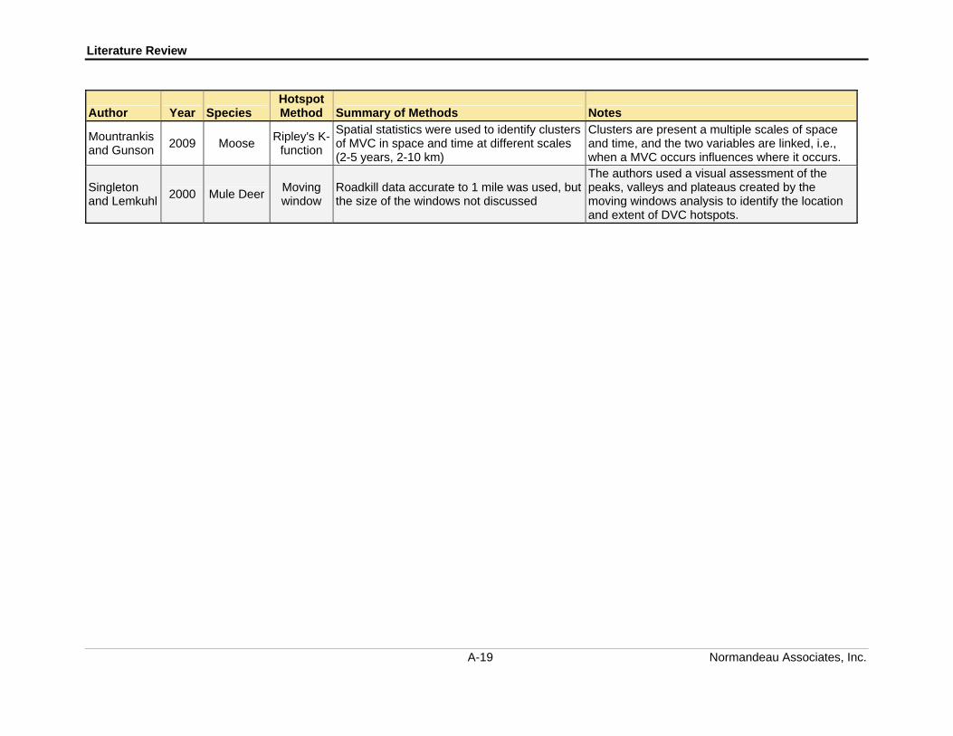
Literature Review

Hotspot Author Year Species

Method Summary of Methods Notes

Mountrankis and Gunson

2009 Moose Ripley's K-

function

Spatial statistics were used to identify clusters of MVC in space and time at different scales (2-5 years, 2-10 km)

Clusters are present a multiple scales of space and time, and the two variables are linked, i.e., when a MVC occurs influences where it occurs.

Singleton and Lemkuhl

2000 Mule Deer Moving window

Roadkill data accurate to 1 mile was used, but the size of the windows not discussed

The authors used a visual assessment of the peaks, valleys and plateaus created by the moving windows analysis to identify the location and extent of DVC hotspots.


Literature Review

Appendix Table A2. Summary of cited DVC/environmental factors methodology references

Author Year Independent

Variable Analysis Method Variables Tested Summary of Results

Species, Data

Source Location

Bashore et al. 1985 hot spot/not a

hot spot logistic

regression 19 variables form the habitat and highway

DVCs positively related to in-line visibility and non-wooded, negatively related to buildings, shortest visibility, speed limit, distance to woods, fencing

White-tail, roadkill

PA, four counties

Bellis and Graves

1971 kills/200 m correlation,

factor analysis

ROW size, veg quality and amount, topography; presence of fence or guardrails

DVC positively related to topography that funnels deer onto the road, and flat areas with good grazing


PA, 8 mile segment of I

80

Biggs et al. 2004 hot spot/not a

hot spot logistic

regression

veg charac, speed limit, road topo, lighting, length of guardrails, height of fence, slope, vis

No individual variable was significant, but slope + veg height fit the data well; taller woody veg and steeper slopes predict hotspots

Mule Deer, DVC

Los Alamos NL, NM

Bissonette and Kassar

2008 # DVC/road

segment regression

rate of DVC to posted speed, AADT

Authors found no relationship between DVCs, speed and AADT - suggest a relationship does exist, but that the scale of measurement between DVC and PSL, AADT was inappropriate

Mule Deer, DVC

UT, statewide

Farrell and Tappe

2007 DVC/County Principle

components, regression

29 landscape, land use, and highway variables reduced to 5 PCs

DVCs increase with increasing urbanization, high edge contrast, lots of edges, and higher deer densities.

White-tail, DVC

AR

Finder et al. 1999 hot spot/not a

hot spot logistic

regression 30 topographic and landscape metrics

DVCs positively related to forest cover, drainages, and public recreation areas; also habitat diversity index when only remotely senses variables considered

White-tail, DVC

IL, statewide

Grovenburg et al.

2008 DVC/County binomial

regression 17 independent varbs and 5 interaction varbs

DVCs positively correlated with secondary roads & hunter success rate; negatively to percent tree cover


eastern SD


Literature Review

Species, Independent Analysis Data

Author Year

Variable Method Variables Tested Summary of Results Source Location

Hubbard et al. 2000 hot spot/not a

hot spot logistic

regression

traffic volume, land cover, dist to city, number of bridge, number of lanes

DVCs associated with large cover-type blocks, drainages

White-tail, DVC

IA, statewide

Iverson and Iverson

1999 DVC/County correlation, regression

DVC to land use variables, human pop, roadway length

Number of DVC/county positively related to amount of urbanization, human population and length of roadway, negatively to amount of crop land

White-tail, DVC

OH, statewide

Malo et al. 2004 hot spot/not a

hot spot logistic

regression 28 habitat, roadway and traffic variables

Local scale: AVCs negatively associated with presence of crossroads, embankments, and guardrails; positively associated with distance to forest.

Roe deer, wild boar, elk, AVC

central Spain

Malo et al. 2004 hot spot/not a

hot spot logistic

regression

% of 8 cover type, ecotone length, habitat diversity

Landscape scale: AVC areas had high tree cover, high diversity and low/no buildings.

Roe deer, wild boar, elk, AVC

central Spain

McShea et al. 2008 DVC/500 m GLM AADT, PSL, road type, cover type, deer density, deer harvest,

DVC most common on two-lane state highways; positively associated with higher traffic volume, and higher housing density on county roads.


Clark County, VA

Ng et al. 2008 DVC site/not a

DVC site logistic

regression

% forested, % non-forested, road density, edge density, distance to forest, water, veg productivity, PSL, AADT

DVCs positively correlated to traffic speed and presence of food.

White-tail, DVC,

Edmonton Alberta

Edmonton, Alberta

Nielsen et al. 2003 hot spot/not a

hot spot logistic

regression 60 metrics describing land use and land cover

DVC areas contained fewer buildings, more patches and a higher proportion of forest cover, more public land patches, and a higher diversity index

White-tail, DVC

Bloomington, MN


Literature Review


Author Year Independent

Variable Analysis Method Variables Tested Summary of Results

Species, Data

Source Location

Puglisi et al. 1974 DVC/mile ANOVA type of fencing, land cover, fence location relative to forest cover

Fence type and location was most important; where no fence was present most DVCs occurred when one side of the highway was forested and the other open field.


PA, I-80

Romin and Bissonette

1996 hot spot/not a

hot spot descriptive, correlation

road topo, ROW width, veg charac, habitat type, traffic volume, traffic speed

DVC areas were positively related to traffic volume, traffic speed, the presence of drainages and the percent woody cover

Mule Deer, roadkill

UT, Wasatch County

Singleton and Lehmkuhl

2000

hotspot compared to

overall habitat availability

t-tests, chi square

median width, % cover, distance to cover, slope, elevation, road density, building density, median type, pavement width, topographic position

DVCs positively associated with lower percent cover, gentler slope, and narrower pavement, lower elevations than generally available and grassy medians. Negatively associated with hillsides and Jersey barrier in the median.

Mule Deer, roadkill

I-90 Snoqualmie Pass, WA

Task 4 Final Report

B-1 Normandeau Associates, Inc.

APPENDIX B – SUMMARY OF CURRENT PRACTICES

Appendix B


EV0103: Investigation of Methods to Identify and Prioritize Deer-Vehicle Crash Locations of Concern – Task 3

Appendix B

This report summarizes the progress of Task 3 of EV0103: Investigation of Methods to Identify and Prioritize Deer-Vehicle Crash Locations of Concern. The goal of Task 3 was to gather information directly from DOTs in order to:

Summarize how states use vehicle crash data to enhance safety

Identify any data sets that can be used to supplement and/or confirm the non-roadway factors believed to impact DVCs

Identify any current practices which are documented to reduce DVC and/or improve the efficiency and quality of DVC data collection

For Task 3, 24 states were chosen for contact in consultation with Mary Gray of the FHWA. These states are listed in Tables 1 and 2. As of June 29, 2010, all states but Arizona responded to requests for a phone interview. Repeated calls and e-mails to various personnel and programs at the Arizona DOT received no response, however information about Arizona’s Wildlife Linkages program was available from the Arizona DOT website. The questions used during the phone interview are attached, and a phone log of each interview conducted is available upon request. The results of the surveys are summarized in Tables 1 and 2.

The methods used by states to identify general crash hotspots along sections of highway are summarized in Table 1. In addition to the phone interviews with DOT personnel, information on analysis of general crash hotspots was gleaned from some state’s “5 Percent Reports” which are required by the FHWA’s Highway Safety Improvement Program. These reports detail the methodologies used to identify the top 5 percent locations in need of safety improvement in each state and are available at http://safety.fhwa.dot.gov/hsip/fivepercent.

Programs varied considerably in methodologies and sophistication. Three states identified high crash locations using a statistically-based modeling approach to determine the expected number of crashes over a given length of roadway. Two states used visual assessments in combination with assessments of rate and frequency, mapping all their crash locations using GIS. All other states used some type of rate, frequency, and/or density measures, often with weighting factors for severity (Table 1). It should be noted that “rate”, “density”, and “frequency” were defined and/or calculated in different ways by different states. Some states had well developed manuals and software written in-house to support their efforts; other states had no specific guidance and used an ad hoc approach. One state (NH) has adopted FHWA’s SafetyAnalyst software to identify its crash hotspots, and one additional state (OH) is currently considering adopting it.

In addition to summarizing the methods used to identify general crash hotspots, Table 1 lists which states conduct analysis to identify DVC hotspots and the type of data, i.e., DVC locations reported on the states’ standardized crash forms or carcass locations, considered to identify DVC hotspots. Most states rely primarily on DVC data from the standard crash form filed by the police responding to a crash (Table 1). The states that do consider carcass data, either alone or combination with DVC data, had a mix of formal and informal carcass recording programs. Maryland had the only fully-developed formal program to record carcass locations. All other formal carcass recording programs were still in the development/pilot phase

Of the 23 states responding, 16 did some type of DVC hotspot analysis, and the responsibility for analysis was split between the Safety (8 states) and the Environmental (6 states) branches, with two DOTs using hotspot analyses conducted by the States’ Fish and Wildlife Departments (Table 2). In all cases, the analyses to identify DVC hotspots conducted by the Environmental branches were visually based, consisting of mapping the DVCs and/or carcasses, then inspecting the maps for concentrations of DVCs. Maryland is part of this group and is noteworthy as it maps and visual analyzes data generated by its Large Animal Removal Reporting System (LARRS), and is the only state contacted that relies on carcass data as its primary data type.

Six of the eight states that gave the analysis responsibility to their Environmental branches or Fish and Wildlife Departments were located in the western US, where deer populations have well-defined migration routes. All the western states contacted for the surveys have developed or are developing state-wide wildlife and habitat linkage analyses, in cooperation with state natural resources agencies and environmental NGOs. The linkage maps created from these analyses provide the primary tool for identifying DVC hotspot locations in these states, augmented to varying degrees with crash data from the Safety branches, and carcass location data from various sources. Expert analysis and traffic volume may also be considered on a project specific basis by some of the western states. All the states which have a linkage analysis available are using deer fencing in combination with underpasses as their primary form of mitigation. Well-maintained fencing is widely accepted to essentially


http://safety.fhwa.dot.gov/hsip/fivepercent

Appendix B

eliminate DVCs, and none of these DOTs were conducting research to determine the efficacy of the mitigation from a safety perspective. Testing to determine the impacts of fencing on animal populations is ongoing.

The over-arching themes of the linkage-based programs appear to be that an ecological process (deer movements) has been acknowledged by these DOTs to cause a significant human safety issue. Once this acknowledgement occurs, the responsibility of understanding this ecological process has been handed off to professional biologists, who are then consulted on a project-specific basis in order to improve safety. This approach appears to have developed in western states due to:

Presence of migratory deer population

Topography that focuses deer movements

Well-developed Environmental branches, that often employ professional biologists

A strong perception by DOT personnel and the general public that deer movements are predictable in time and space, which creates support and demand for mitigation measures

Of the eight Safety branches that conducted the analyses to identify DVC hotspots, Maine, Iowa, and Ohio had formal programs (discussed briefly below), while the remaining five conducted analysis informally and/or at the request of districts. A variety of analysis methods were used, including visual analysis of mapped data, and comparisons of frequency or rate over a section. Maine, Ohio, and Alabama used the same approach with DVC that they used with other types of crashes, but the other five states used a less rigorous approach with their DVC data, as compared to their general crash data.

Of the eastern DOTs, Maine had the most developed DVC hotspot analysis program. DVC and moose-vehicle collision hotspots are identified in each region by season and time of day using the same map-based, visual techniques that the MDOT Safety Office uses for all its crash data. Once hotspots are identified, non-roadway factors, especially the location of deer wintering areas, are then considered to help develop the best mitigation approach. Mitigation approaches used by MDOT include passive and active signage, seasonal signage, wide striping to provide greater contrast for drivers to see deer against the dark roadway, mirrors angled to illuminate the roadside to help drivers see deer on the roadside, and rip-rap on the roadside to slow down and discourage passage by deer. Additionally, Maine has a well-developed DVC public awareness campaign, and fencing and underpasses are being considered for new construction and major reconstruction projects. MDOT is currently testing the efficacy of some of these methods. Results are mixed so far, due in part to small sample sizes.

The Ohio DOT Office of Systems Planning and Program Management examines its DVC data on a yearly basis, in the fall, to coincide with its annual DVC awareness campaign, which is timed to coincide with an increase in deer activity due to the rut. Like crashes in general, ODOT considers the rate and frequency of DVC over two mile sections to identify hotspots. However, ODOT is testing SafetyAnalyst this year and may make the switch if it compares favorably with its current methods. In addition to noting high-hazard location in awareness campaigns, ODOT also uses hotspot information to locate signage and focus vegetation management efforts. Hotspot locations are mapped using GIS and combined with high resolution aerial photography to identify habitat characteristic (e.g. sharp breaks in cover type from open to forest) to refine the placement of signs and focus the vegetation management efforts. ODOT does not doing any testing to determine the efficacy of its mitigation efforts.

The Iowa DOT maps all DVC and uses a visual analysis to identify hotspots, but uses a non-visual, density based analysis for hotspot analysis of general crashes. In addition to reported DVC, carcass data may also be considered to identify DVC hotspots. Fencing is the primary form of mitigation IDOT undertakes, using existing bridges and culverts to provide passage for deer across fenced sections. Although DVC hotspots can be identified, DVC in Iowa are very widespread. Choosing a location to install fencing is based primarily on a project-specific cost/benefit and the presence of land use or topographic features that give the fence logical termini. Before and after crash data from two recent fencing projects indicate an almost complete elimination of DVC along the fenced segments.

All of the seven states that did not do any formal analysis to identify the locations of DVC hotspots were located in the East or Upper Midwest (Table 1). Two of these states (IL, WI) remove deer crashes from their analysis of general crash hotspots because they believe DVC to be random. The contacts from Georgia, North Carolina, and Nebraska expressed that their informal analyses has not revealed a discernable pattern in DVCs, and that it was


Appendix B

difficult to identify DVC hotspots. However, despite a belief that DVC occur randomly, all states indicated that they do believe DVC are a significant safety issue, and the NC and WI DOTs do conduct DVC awareness campaigns annually during autumn. Aside from these two awareness campaigns, none of the other five states that do not conduct formal analysis of DVC hotspots had a formal program of countermeasures to reduce DVC. Two states (NH, MN) noted that DVC may be identified as the primary contributor to a crash hotspot during general hotspot analysis, and that signage or vegetation management might be implemented in these locations as countermeasures on an ad hoc basis.

In summary, the following primary trends were noted:

1. The most common method to identify the location of DVC hotspots was to map DVC locations and use a simple visual analysis.

2. No DOT’s interviewed were using model-based analyses or spatial statistics to identify the location of DVC hotspots.

3. Testing to determine the efficacy of DVC mitigation methods was uncommon.

4. Formal, well developed programs to identify DVC hotspots were most commonly conducted by a professional biologist located in either a DOT’s Environmental branch or the state’s Fish and Wildlife Department.

5. Formal, well developed programs to identify DVC hotspots were all associated with states where distinct season movements of deer and well defined topographic features combine to focus deer movements.

6. Habitat linkage models, developed by partnerships of State DOTs, Natural Resource Agencies, and NGOs, are the non-roadway data most commonly considered to help locate DVC hotspots.

7. Safety personnel rarely used non-roadway data to help identify DVC hotspots.

8. States that have analyzed data and have difficulty identifying DVC hotspots are predominantly southern and/or relatively flat. Lack of seasonal movements by deer, and topographic features to focus deer movements appears to result in a diffuse pattern of DVCs.

9. DVCs are perceived to be a safety hazard in all states, including those where the safety branch personnel feel that DVC hotspots can not readily be defined.

Questions Asked During Interviews of Dot Safety and Environmental Personnel

Describe How You Use Vehicle Crash Data to Enhance Safety

1. What Department or Group is responsible for analyzing crash data to identify locations in need of safety improvements?

2. Briefly describe how crash data is analyzed to identify locations in need of safety improvements.

3. Do you have specialized software or a write specific code for crash analysis?

4. Do you have a written protocol for hotspot ID? Can you send it to me?

5. How often do you look for hotspots and at what scale?

6. Do you have a specific threshold for recommending safety improvements?

7. Do you conduct analysis to determine if safety improvements have the desired effect?

8. What type of analysis do you use to determine if safety improvements have the desired effect?

9. Do you subdivide your accident data (e.g., motorcycles, pedestrians, animals) for analysis?

Questions for any States that analyze DVC separately from other accident types.

10. Do you collect DVC data from sources other than accident forms?

11. How do you identify DVC hotspots?


Appendix B


12. Do you use DVC hotspot analysis to make operational recommendations to improve safety? What sort of operational recommendations do you make? Signage, fencing, awareness campaigns, etc.

13. Have you/will you conducted any analysis to determine if these recommendations have the desired effect? What type of analysis will you use to determine if the recommendation have the desired effect?

14. Do you do any type of analysis to link DVC hotspots (or other hotspots) to non-roadway factors?

15. What type of data set do you use to represent the non-roadway factors?

Appendix B

Table 1. Summary of interview results relating to analysis of general crash hotspots and data collection. States are sorted by analysis

method used to identify general crash hotspots.

State* General Method Animal Check Box on Standard Crash

Form

Analyze DVC?

Who does DVC analysis?

Data used for DVC Analysis

Carcass Program

CO Binomial model Wild yes Enviro DVC, carcasses formal

IL Binomial model Deer no na na no

IA Density Animal yes Safety DVC formal

FL Frequency Animal no na na no

AL Frequency Animal yes Safety DVC no

AZ Frequency Animal, wild _____ yes Enviro ? ?

UT Frequency Wild yes Enviro DVC formal

NC Frequency, Density Animal no na na no

NB Frequency, Rate Animal yes Safety DVC no

TX Rate Animal no na na no

CT Rate Deer no na na no

CA Rate Animal _______ yes Enviro DVC, carcasses informal

ID Rate wild animal yes DNR carcasses informal

MD Rate Animal yes Enviro carcasses formal

NY Rate Deer yes Enviro DVC formal

PA Rate Deer yes Safety DVC no

WA Rate Deer yes DNR carcasses formal

NH SafetyAnalyst Deer no na na no

OH Various - density, rate, frequency Deer yes Safety DVC formal

MN Various - severity, rate, frequency Deer no na na no

WI Various - severity, rate, frequency Deer no na na formal

GA Various - severity, rate, frequency Animal yes Safety DVC no

ME Visual Deer yes Safety DVC informal

VA Visual Deer yes Safety DVC informal

*States in Bold are Pooled Fund States B-7 Normandeau Associates, Inc.

Appendix B


Table 2. Summary of interview results relating to analysis of DVC hotspots. States are sorted by name of the DOT branch that conducts

DVC hotspot analysis.

State Who does DVC

Analysis? DVC Hotspot

Method In-house

Biologist? Habitat Linkage

Program? Non-roadway Factors

Considered? Mitigation Program?

ID DNR Expert opinion No yes Linkages Fencing, underpasses

WA DNR Visual Yes yes Linkages Fencing, underpasses

AZ Enviro ? Yes yes Linkages Fencing, underpasses

CA Enviro Visual, expert

opinion Yes yes Linkages Fencing, underpasses

CO Enviro Visual Yes yes Topo, migration routes Fencing, underpasses

MD Enviro Visual No no Topo, vegetation Signage

NY Enviro Visual Yes no Food sources Awareness campaigns

UT Enviro Visual Yes yes Migration routes Fencing, underpasses

CT na na No no no Informal

FL na na No no no no

IL na na No no no no

MN na na No no no Signage

NC na na No no no Awareness campaigns

NH na na No no no no

TX na na yes no no no

WI na na No no no Awareness campaigns

AL Safety Frequency No no no local

GA Safety Frequency No no no no

IA Safety Visual No no no Fencing

ME Safety Visual No no Wintering locations Various

NB Safety Frequency No no no Signage, veg control

OH Safety Rate, frequency,

density No no Vegetation Awareness campaigns, veg control

PA Safety Rate No no no Fencing, awareness

VA Safety Visual No no no Signage

*States in Bold are Pooled Fund States

Task 4 Final Report

C-1 Normandeau Associates, Inc.

APPENDIX C - FIGURES

Appendix C

Appendix Figure C-1. Iowa Locus Map.


Appendix C


Appendix Figure C-2. New York Locus Map.

Appendix C


Appendix Figure C-3. Comparison of map types for visual analysis.

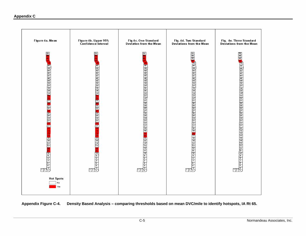
Appendix C


Appendix Figure C-4. Density Based Analysis – comparing thresholds based on mean DVC/mile to identify hotspots, IA Rt 65.

Appendix C


Appendix Figure C-5. Route 65 hotspots identified using a binomial model (95% CI) and a three-mile moving window based on the binomial model.

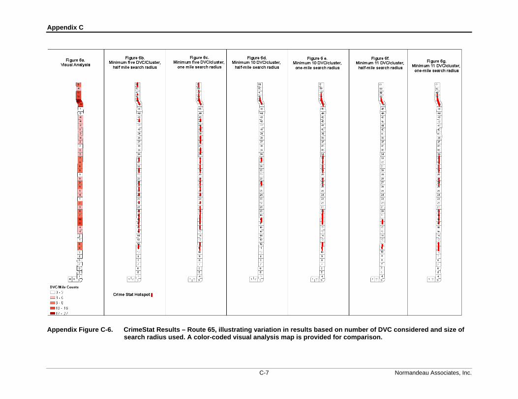
Appendix C


Appendix Figure C-6. CrimeStat Results – Route 65, illustrating variation in results based on number of DVC considered and size of search radius used. A color-coded visual analysis map is provided for comparison.

Appendix C

Appendix Figure C-7. Data (map) used for the expert analysis, Iowa Route 65.


Appendix C

Appendix Figure C-8. Iowa I-35 Results. Figure 8a segments are labeled by DVC count; all others are labeled by segment number.


Appendix C

Appendix Figure C-9. Iowa Route 65 Results. 9a segments are labeled by DVC count; all others are labeled by segment number.


Appendix C

Appendix Figure C-10. New York I-90 Results. 10a segments are labeled by DVC count; all others are labeled by segment number.


Appendix C


Appendix Figure C-11. NY Route 28 Result. 11a segments are labeled by DVC count; all others are labeled by segment number.

methods to identify and prioritize deer locations.pdfdvc/mile to identify hotspots, ... gaps, the...

Documents