methodology for estimating life expectancies of highway … 08-71... · i methodology for...
TRANSCRIPT

i
Methodology for
Estimating Life Expectancies of Highway Assets
DRAFT FINAL REPORT
Kevin M. Ford, Mohammad Arman, Samuel Labi, Kumares C. Sinha,
Arun Shirole, Paul Thompson, Zongzhi Li
School of Civil Engineering Purdue University
West Lafayette, IN 47907
June 10, 2011
NCHRP 08-71
Transportation Research Board NAS-NRC
Limited Use Document This document is for use by the National Highway Cooperative
Research Program. Dissemination of the information included therein must be approved by the NCHRP.

ii
ACKNOWLEDGMENTS
The research team acknowledges the valuable support and guidance of Dr. Andrew Lemer, the project manager and the entire NCHRP 08-71 Project Panel: Mark Nelson, Minnesota DOT (Panel Chair), Lacy Love, NCDOT (AASHTO Monitor), Gerardo Flintsch, Virginia Tech, Sheila Moore, TRB, Michael Plunkett, PowerPlan Consultants, Raymond Tritt, Caltrans, Nastaran Saadatmand, FHWA (FHWA Liaison), Nadarajah “Siva” Sivaneswaran, FHWA (FHWA Liaison), Don Clotfelters, Washington DOT, and Eric Pitts, Georgia DOT.
We also acknowledge the efforts of team member George Stamm of Om Popli Inc., and the following individuals who shared data and knowledge on state highway asset inventory and performance: Ocie Adams (AK), Gregory Lockshaw, Wes Lum, Ray Tritt, and Eric Uyeno (CA); Scott Neubauer (IA); Darcy Bullock (IN); Nancy Albright, Ted Swansegar, Jon Wilcoxson, and Jeff Wolfe (KY); John Smith and John Vance (MI); Thomas Martin, Mark Nelson, and Bonnie Peterson (MN); James Burke and Li Zhang (MS); Jane Berger (ND); James Bledsoe, Joseph Jones, and David Nichols (MO); John Dourgarian and David Kuhn (NJ); Lou Adams, Michael Fay, and Scott Lagace (NY); Ginger McGovern (OK); John Coplantz, Joel Fry, Laura Hansen, Bert Hartmann, Bill Link, Carol Newvine, Marina Orlando, Mark Wills (OR); Janice Arellano, Daniel Farley, David Kuniega, Michael Long, and John Van Sickle (PA); Jennifer Brandenburg, Steve Dewitt, and Kevin Lacy (NC); David Chan (NY); Paul Annarummo, Kazem Farhoumand, and Bob Rocchio (RI); Dave Huft (SD); Larry Buttler, Rick Collins, Brian Merrill, Steve Simmons, Bryan Stampley, Brian Stanford, and Tom Yarbrough (TX); Michael Fazio, Ahmad Jaber, and Brant Whiting (UT); Tanveer Chowdhury, Brack Dunn, and Raja Shekharan (VA); David Luhr (WA), and Martin Kidner (WY).
The contributions of Michelle Dojutrek and Eleni Bardaka, graduate research assistants at Purdue University, were very significant, particularly in the demonstration of pavement life expectancy estimation techniques and application of service life estimates in asset valuation.

iii
TABLE OF CONTENTS Page
CHAPTER 1 INTRODUCTION................................................................................... 1 1.1 Role of Highway Asset Life Expectancy in Business Processes............... 1
1.2 Rationale for Highway Asset Replacement and Retirement...................... 3 1.3 Uncertainty in Life Expectancy Estimation and Related Business Processes.................................................................................................. 4 1.4 Study Objectives........................................................................................ 7 1.5 Organization of the Report......................................................................... 7
CHAPTER 2 METHODOLOGIES FOR LIFE EXPECTANCY ESTIMAT ION........ 8
2.1 Literature Review of Life Expectancy Practices......................................... 8 2.1.1 Definitions and Measures of Asset Life Expectancy............................... 8 2.1.2 Measures of Asset Life………………....................................................... 9 2.1.3 Established Life Expectancy Values....................................................... 9 2.1.3.1 Bridge Life Estimates........................................................................... 10 2.1.3.2 Culvert Life Estimates.......................................................................... 11 2.1.3.3 Traffic Sign Life Estimates................................................................... 13 2.1.3.4 Pavement Marking Life Estimates....................................................... 14 2.1.3.5 Pavement Life Estimates..................................................................... 14 2.1.3.6 Traffic Signal Life Estimates................................................................ 15 2.1.3.7 Roadway Lighting Life Estimates......................................................... 16 2.1.4 Methods for Estimating Life Expectancy........... 17 2.1.4.1 Mechanistic Methods for Estimating Life Expectancy.......................... 17 2.1.4.2 Empirical Methods for Estimating Life Expectancy.............................. 22 2.2 Methodologies for Estimating Asset Life.................................................... 23 2.2.1 Identify Replacement Rationale.............................................................. 24 2.2.2 Define End-of-Life................................................................................... 24 2.2.3 Select General Approach........................................................................ 24 2.2.3.1 Expert Opinion or Published Life Expectancy Values.......................... 24 2.2.3.2 Condition-based Approach.................................................................. 24 2.2.3.3 Age-based Approach........................................................................... 25 2.2.3.4 Condition/Age-based Hybrid Approach................................................ 26 2.2.4 Select Modeling Technique..................................................................... 26 2.2.4.1 Regression Models.............................................................................. 27 2.2.4.2 Neural Networks.................................................................................. 28 2.2.4.3 Ordered Discrete Response Models.................................................... 29 2.2.4.4 Markov Chains..................................................................................... 31 2.2.4.5 Duration Models................................................................................... 32 2.2.4.6 Markov-based Duration Models........................................................... 36 2.2.5 Model Selection Recommendations....................................................... 38 2.2.6 Data Availability Assessment and Grouping of Data.............................. 38 2.2.7 Incorporating Maintenance Frequencies and Intensities into Life Expectancy Models................................................................... 39 2.3 Chapter Summary...................................................................................... 41

iv
Page
CHAPTER 3 APPLICATION OF THE METHODOLOGIES FOR LIFE EXPECTANCY ESTIMATION ....... ....................................................... 42
3.1 Introduction......................................................................................... 42 3.2 Data Collection.................................................. 42 3.2.1 Asset-specific Data................................................................................. 42 3.2.1.1 Bridge Data.......................................................................................... 42 3.2.1.2 Box Culvert Data.................................................................................. 44 3.2.1.3 Pipe Culvert Data................................................................................. 45 3.2.1.4 Pavement Data.................................................................................... 45 3.2.1.5 Traffic Sign Data.................................................................................. 45 3.2.1.6 Pavement Marking Data...................................................................... 46 3.2.1.7 Roadway Lighting Data........................................................................ 47 3.2.1.8 Traffic Signal Data............................................................................... 47 3.2.1.9 Flasher Data........................................................................................ 48 3.2.2 Environmental Data................................................................................ 48 3.3 Results........................................................................................................ 49 3.3.1 Bridges....................................................................................................... 49 3.3.2 Culverts...................................................................................................... 49 3.3.3 Box Culverts............................................................................................ 65 3.3.4 Pipe Culverts........................................................................................... 71 3.3.5 Traffic Signals............................................................................................ 72 3.3.6 Flashers..................................................................................................... 75 3.3.7 Roadway Lighting...................................................................................... 76 3.3.8 Traffic Signs............................................................................................... 77 3.3.9 Pavement Markings................................................................................... 78 3.3.10 Pavements................................................................................................. 78 3.4 Summary of Life Expectancy Estimates Calibrated to Collected Data........................................................................................................... 80
CHAPTER 4 INCORPORATING LIFE EXPECTANCY ESTIMATES I NTO ASSET MANAGEMENT FUNCTIONS........................ ......................... 83
4.1 Fundamental Life Expectancy Applications............................................... 83 4.1.1 Evaluating Replacement and Life Extension Activities Using LCCA...... 83 4.1.1.1 Brief History of LCCA........................................................................... 83 4.1.1.2 LCCA Analysis Period and Asset Life Expectancy Relationship......... 84 4.1.1.3 LCCA Techniques................................................................................ 88 4.1.1.4 Life Expectancy Applications in LCCA................................................. 89 4.1.1 Asset Valuation Based on Asset Life Expectancy.................................. 90 4.1.2 Ranking Replacement and Life Extension Activities Using Utility Theory........................................................................................... 91 4.1.3 Budgeting for Asset Replacement.......................................................... 93 4.2 Example Calculations Involving Asset Life Expectancy............................. 93 4.2.1 LCCA Calculations Involving Asset Life Expectancy.............................. 93 4.2.1.1 Example Calculations of Basic LCCA Measures................................. 94

v
Page 4.2.1.2 Example LCCA Calculations for Comparing Alternative Preservation Activities.......................................................................... 97 4.2.1.3 Example LCCA Calculations for Justifying Routine
Preventative Maintenance.................................................................... 98 4.2.1.4 Example LCCA Calculations for Identifying the Optimal
Replacement Interval........................................................................... 98 4.2.1.5 Example LCCA Calculations for Comparing Design Alternatives........ 100 4.2.1.6 Example LCCA Calculations for Comparing Life Extension
Alternatives.......................................................................................... 100 4.2.1.7 Example LCCA Calculations for Pricing Design and
Preservation Alternatives..................................................................... 102 4.2.1.8 Example LCCA Calculations for Synchronizing Replacements........... 103 4.2.1.9 Example LCCA Calculations for Assessing the Value of Life
Expectancy Information........................................................................ 104 4.2.2 Asset Valuation Based on Asset Life Expectancy.................................. 105 4.2.3 Utility Calculations Involving Asset Life Expectancy............................... 106 4.2.4 Budget Calculations Involving Asset Life Expectancy............................ 106 4.3 Summary of Life Expectancy Applications................................................. 106
CHAPTER 5 METHODS TO ACCOUNT FOR ASSET LIFE UNCERTA INTY IN ASSET
REPLACEMENT DECISIONS.............................. ................................ 107 5.1 Rationale for Incorporating Risk Into Long-term Planning......................... 107 5.2. Overview of Uncertainty Analysis............................................................. 108 5.2.1 Describing Values with Set Theory......................................................... 108 5.2.2 Uncertainty Types................................................................................... 109 5.2.3 Likelihood Representations..................................................................... 109 5.2.4 Distribution Fitting................................................................................... 110 5.2.5 Sampling Distributions............................................................................ 110 5.2.6 Representing Output Uncertainty............................................................ 114 5.2.7 Decision Making Under Uncertainty........................................................ 114 5.2.8 Review of Sensitivity Analysis................................................................. 115 5.2.9 Review of Risk Analysis.......................................................................... 118 5.3 Literature Review of Risk Studies in Transportation Engineering.............. 119 5.4 Methodology for Assessing the Risk of Uncertain Service Life Estimates in Long-Term Planning Decisions............................................. 112 5.4.1 Risk Identification.................................................................................... 112 5.4.1.1 Risk of Uncertain Future Climate......................................................... 123 5.4.1.2 Risk of Inaccurate Needs Assessment................................................ 124 5.4.2 Risk Assessment.................................................................................... 124 5.4.2.1 Predicting Life Expectancy Based on Uncertain Inputs....................... 124 5.4.2.2 Predicting Budget Needs Based on Uncertain Life Expectancy
Estimates............................................................................................. 125 5.4.2.3 Comparing Replacement Policies........................................................ 126 5.4.3 Risk Management................................................................................... 127 5.4.3.1 Mitigation Strategies............................................................................ 127 5.4.3.2 Setting Risk Tolerance......................................................................... 127 5.4.4 Risk Monitoring....................................................................................... 127 5.5 Summary of Uncertainty Assessments...................................................... 127
vi
Page
CHAPTER 7 INCORPORATING UNCERTAINTY IN ASSET REPLAC EMENT DECISIONS.................................................................................................... 128
6.1 Overview of Uncertainty Assessments on Developed Models................... 128 6.2 Sensitivity Analysis of Developed Models.................................................. 128 6.2.1 Sensitivity of Bridge Life Prediction......................................................... 128 6.2.2 Sensitivity of Box Culvert Life Prediction................................................ 137 6.2.3 Sensitivity of Pipe Culvert Life Prediction............................................... 141 6.2.4 Sensitivity of Traffic Signal Life Prediction.............................................. 142 6.2.5 Sensitivity of Flasher Life Prediction....................................................... 142 6.2.6 Sensitivity of Roadway Lighting Life Prediction...................................... 143 6.2.7 Summary of Sensitivity Analyses............................................................ 144 6.3 Risk Assessments of Highway Asset Replacement Decisions.................. 144 6.3.1 Risk of Uncertain Future Climate............................................................ 144 6.3.1.1 Risk Assessment of Uncertain Future Climate on Bridge Life............. 147 6.3.1.2 Risk Assessment of Uncertain Future Climate on Box Culvert Life..... 149 6.3.1.3 Risk Assessment of Uncertain Future Climate on Pipe Culvert Life.... 151 6.3.1.4 Risk Assessment of Uncertain Future Climate on Traffic Signal Life... 153 6.3.1.5 Risk Assessment of Uncertain Future Climate on Flasher Life............ 155 6.3.1.6 Risk Assessment of Uncertain Future Climate on Roadway
Lighting Life.......................................................................................... 157 6.3.2 Risk-based Needs Assessment.............................................................. 159 6.3.2.1 Hybrid Age/Condition-based, Probabilistic Needs Assessment........... 160 6.3.2.2 Condition-based, Probabilistic Needs Assessment............................. 163 6.3.2.3 Deterministic Needs Assessments...................................................... 170 6.3.2 Summary................................................................................................. 174
CHAPTER 7 SUMMARY AND CONCLUSIONS.................. .................................... 178
7.1 Study Overview.......................................................................................... 178 7.2 Life Expectancy Modeling.......................................................................... 178 7.3 Use of Life Expectancies in Highway Asset Management Decisions........ 178 7.4 Accounting for Uncertainties in Asset Replacement Decisions................. 178 7.5 Areas of Future Research.......................................................................... 180
LIST OF REFERENCES............................................................................................ 181 APPENDICES............................................................................................................ 216 A. Definitions of Life Expectancy Condition/Performance Measures....................... 217 B. Bridge Markov/Weibull Results by Element, Region, and ‘Failure Mechanism’.... 232 C. Box Culvert Markov/Weibull Results by State and ‘Failure Mechanism’............ 280 D. Interest Formulae for LCCA................................................................................ 292

vii
LIST OF TABLES Table Page 2-1: Survey Results for Culvert Life Expectancy Estimates for Pipe and Box Culverts (Markow, 2007).............................................................................. 12 2-2: 2003 Survey of Life Expectancy Estimates for Pipe Culverts (Perrin Jr. & Jhaveri, 2004)...................................................................................................... 12 2-3: Oregon Traffic Sign Service Life Estimates by Sign Sheeting and Retroreflectivity Thresholds (Kirk et al., 2001)..................................................... 13 2-4: Survey of Life Expectancy Estimates for Traffic Signals (Markow, 2007)........... 15 2-5: Survey of Life Expectancy Estimates for Roadway Lighting (Markow, 2007).................................................................................................... 16 2-6: Mechanistic Methods for Predicting the Life of Concrete Structures (Liang et al., 2002)............................................................................................... 17 2-7: Prediction of Corrosion Time Stages (Liang, Lin, & Liang, 2002)........................ 20 2-8: Representations of Probability............................................................................. 32 3-1: Data Statistics for Condition-based Bridge Life................................................... 44 3-2: Data Statistics for Inteval-based and Condition-based Box Culvert Life............. 45 3-3: Data Statistics for Assumed Pipe Culvert Life..................................................... 46 3-4: Data Statistics for Historical Roadway Lighting Life............................................ 47 3-5: Data Statistics for Historical Traffic Signal Life.................................................... 48 3-6: Data Statistics for Historical Flasher Life............................................................. 48 3-7: Weibull Regression Model of Bridge Service Life (End-of-life ≡ Age when Sufficiency Rating drops to or below 50%)......................................... 52 3-8: Bridge Deck Transition Matrices for All Observations......................................... 54 3-9: Bridge Superstructure Transition Matrices for All Observations.......................... 54 3.10: Bridge Substructure Transition Matrices for All Observations............................. 55 3-11: Bridge Deck Geometry Transition Matrices for All Observations........................ 56 3-12: Bridge Channel Protection Transition Matrices for All Observations................... 56 3-13: Bridge Scour Protection Transition Matrices for All Observations....................... 57 3-14: Number of Observations used in Developing Bridge Deck Transition Matrices............................................................................................................... 57 3-15: Number of Observations used in Developing Bridge Superstructure Transition Matrices............................................................................................. 57 3.16: Number of Observations used in Developing Bridge Substructure Transition Matrices............................................................................................ 58 3-17: Number of Observations used in Developing Bridge Deck Geometry Transition Matrices............................................................................................ 58 3-18: Number of Observations used in Developing Bridge Channel Protection Transition Matrices............................................................................................ 59 3.19: Number of Observations used in Developing Bridge Scour Protection Transition Matrices............................................................................................ 59 3-20: Markov/Weibull Model Predictions of Bridge Service Life by Failure Mechanism for All Observations........................................................................ 60 3-21: Markov/Weibull Model Predictions of Bridge Service Life by Failure Mechanism and SHRP-LTPP Region................................................................ 62 3.22: Weibull Regression Model of Box Culvert Service Life (End-of-life ≡ Historical Replacement Interval and Age when Culvert Condition Rating drops to or below 3)........................................................................................... 66

viii
Table Page 3-23: Box Culvert Condition Transition Matrices for All Observations........................ 67 3-24: Box Culvert Channel Protection Transition Matrices for All Observations......... 67 3-25: Number of Observations used in Developing Box Culvert Condition Transition Matrices............................................................................................. 68 3-26: Number of Observations used in Developing Box Culvert Channel Protection Transition Matrices........................................................................... 68 3-27: Markov/Weibull Model Predictions of Box Culvert Service Life by Failure Mechanism for All Observations....................................................... 69 3-28: Markov/Weibull Model Predictions of Box Culvert Service Life by Failure Mechanism and SHRP-LTPP Region.................................................... 70 3-29: Log-Logistic Regression Model of Pipe Culvert Service Life (End-of-life ≡ Age of Assets with Physical or Structural Condition Rating of 3, Flow rating of 2, or Roadway Deflection > 1”)........................................................... 72 3-30: Log-Logistic Regression Model of Traffic Signal Service Life (End-of-life ≡ Historical Replacement Interval)................................................... 73 3-31: Weibull Regression Model of Flasher Service Life (End-of-life ≡ Historical Replacement Interval)........................................................................ 74 3-32: Weibull Regression Model of Roadway Lighting Service Life (End-of-life ≡ Historical Replacement Interval)................................................... 77 3-33: Example Transition Matrix for Simple Markov Model, Traffic Signs ………..... 76 3-34: Markov Model for pavement Resurafcing ……………………………………… 80 3-35: Summary of Asset Service Life Model Predictions............................................ 81 3.36: Summary of Asset Life Model Statistics............................................................ 82 4-1: Example Comparison of Life-Cycle Activity Profiles in Evaluating the Benefit or Disbenefits of Conducting Routine Preventative Maintenance.......... 98 4-2: Example Data for Optimizing Replacement and Maintenance Activity Intervals. 99 4-3: Example Bridge Life Extension Alternatives........................................................ 101 4-4: Example data for synchronizing replacement intervals....................................... 103 4-5: Example ranked projects with associated utility and cost.................................... 105 4-6: Example Needs Assessment Data...................................................................... 106 5-1 Risk Assessment Methods (Ayyub, 2003)............................................................ 118 5-2: Classification of Past Risk Analyses.................................................................... 120 6-1: Range of Bridge Life Values for Covariate Model Sensitivity Analysis................ 128 6-2: Bridge Median Life Predictions by End-of-Life Definition and Data Segmentation....................................................................................................... 129 6-3: Range of Box Culvert Life Values for Covariate Model Sensitivity Analysis........ 137 6-4: Box Culvert Median Life Predictions by End-of-Life Definition and Data Segmentation....................................................................................... 138 6-5: Range of Pipe Culvert Life Values for Covariate Model Sensitivity Analysis....... 141 6-6: Range of Traffic Signal Life Values for Covariate Model Sensitivity Analysis..... 142 6-7: Range of Flasher Life Values for Covariate Model Sensitivity Analysis.............. 142 6-8: Range of Roadway Lighting Life Values for Covariate Model Sensitivity Analysis 143 6-9: Assumed Bridge Replacement Costs (Sinha et al., 2009)................................. 159 6-10: Correlation Matrix of Remaining Indiana Deck, Superstructure, and Substructure Life................................................................................................ 163 6-11: Assumed Deck Replacement, Superstructure Rehabilitation, and Substructure Rehabilitation Costs (Sinha et al., 2009)...................................... 167 6-12: Risk of Underestimating Long-term Fiscal Needs by Scenario if Assume 60 Year Life for All Structures............................................................................ 170

ix
Table Page 6-13: Summary of One-way Sensitivity Analysis of Climate Conditions for Typical Project-level Characteristics.................................................................. 174 6-14: Summary of Probabilistic Risk Analysis of Climate Conditions for Typical Project-level Characteristics............................................................................. 175 6-15: Comparison of Risk-based and Deterministic Needs Assessments for Indiana Bridges over 2009-2023 Planning Horizon........................................... 176 Appendix Tables 178

x
LIST OF FIGURES
Figure Page 1-1: Applications of Life Expectancy in Asset Management Processes........................ 2 1-2: Probabilistic Considerations at Various Phases of Asset Development................. 3 1-3: Role of Uncertainty in Long-range Planning (Thompson et al., 2011….................. 5 2-1: Illustration showing the Different Definitions of Asset Life........................................ 9 2-2: General Methodology for Estimating Highway Asset Life Expectancy.................... 23 2-3: Condition-based life expectancy (Conceptual Illustration) (Thompson et al., 2011)............................................................................................. 25 2-4: Age-based life expectancy (Conceptual Illustration)................................................ 25 2-5: Example of an Artificial Neural Network................................................................... 28 2-6: Example illustration of a 3-state ordered probit model (Washington et al., 2003) 30 2-7: Example Markov Chain Graph and Transition Matrix.............................................. 31 2-8: Asset Survival Curves using Different Performance Indicators and Performance Thresholds (Irfan et al., 2009)............................................................. 33 2-9: Censoring Types in Duration Modeling (Washington et al., 2003)........................... 35 2-10: General Procedure for Selection of Life Expectancy Model.................................. 38 2-11: Example Dendrogram developed using Cluster Analysis........................................ 39 2-12: Incorporating the Effect of Maintenance on Asset Performance (Labi, 2001)....... 40 3-1: United States Climate Divisions used by the NOAA (NOAA – Most Popular Products/Free Data)............................................................................ 49 3-2: SHRP-LTPP Climate Regions.................................................................................. 50 3-3: Non-parametric Validation of Weibull-distributed Bridge Life Covariate Model…… 51 3-4: Bridge Deck Median RSL by Age and Current Rating......................................... 62 3-5: Bridge Superstructure Median RSL by Age and Current Rating......................... 63 3-6: Bridge Substructure Median RSL by Age and Current Rating............................ 63 3-7: Bridge Deck Geometry Median RSL by Age and Current Rating........................ 64 3-8: Bridge Channel Protection Median RSL by Age and Current Rating.................. 64 3-9: Bridge Scour Protection Median RSL by Age and Current Rating...................... 65 3-10: Non-parametric Validation of Weibull-distributed Box Culvert Life Covariate Model................................................................................................... 66 3-11: Box Culvert Condition Median RSL by Age and Current Rating....................... 70 3-12: Box Culvert Channel Rating Median RSL by Age and Current Rating.............. 70 3-13: Non-parametric Validation of Log-Logistic-distributed Pipe Culvert Life Model.................................................................................................................. 71 3-14: Non-parametric Validation of Log-Logistic-distributed Traffic Signal Life Model 73 3-15: Non-parametric Validation of Weibull-distributed Flasher Life Model................ 74 3-16: Non-parametric Validation of Weibull-distributed Roadway Lightign Life Model 75 3-17: Example Life Expectancy Estimate of Traffic signs….…………………………… 77 3-18: Example life expectancy estimate of 1A: 2-yr Water-based Yellow Pavement
Marking ……………………………………………………………………………… 78 3-19: Survival Curve (Kaplan-Meier method) for hot-mix asphalt concrete pavements 78 3-20: Example life expectancy estimate of pavements treated with resurfacing……… 80 4-1: Analysis Period for Existing and New Assets...................................................... 85 4 2: Scenarios for Analysis Period Length relative to Overall Life, New Assets......... 86 4-3: Scenarios for Analysis Period Length relative to Remaining Life, Existing Assets.. 87 4-4: Perpetual Life-cycle Profile for a Typical Highway Asset.................................... 89 4-5: General Remaining Service Life Utility Curve (Li & Sinha, 2004)........................ 91

xi
4-6: Bridge Remaining Service Life Utility Curve (Sinha et al., 2009)........................ 92 4-7: Example Activity Profiles for Carbon Steel and Stainless Steel Options (Cope, 2009)......................................................................................................... 102 4-8: Example Asset Valuation using Highway Asset Life Expectancy........................ 105 5-1: Example of Classical (Crisp), Fuzzy, and Rough Values.................................... 109 5-2: Statistical Copula Correlation Patterns (Vose Software, 2007)........................... 113 5-3: Value Function using Prospect Theory (Kahneman & Tversky, 1979)................ 114 5-4: Defining Risk Value with Utility Curves (Sinha & Labi, 2007).............................. 115 5-5: Example of a Tornado Diagram (Molenaar et al., 2006)..................................... 116 5-6: Example of a Spider Diagram (van Dorp, 2009).................................................. 116 5-7: Monte Carlo Simulation Process (van Dorp, 2009)............................................. 119 5-8: Example Management System (Morcous et al., 2010)........................................ 120 5-9: General Methodology for Assessing Uncertainty................................................ 122 5-10: Multiple 2050 Temperature Change Projections Relative to Current Climate (Solomon, et al., 2007)............................................................. 123 5-11: Competing Risk Models (Peter e al., 2002)....................................................... 126 6-1: Tornado Diagram of Covariate Bridge Life Model............................................... 129 6-2: Sensitivity of Non-Covariate Indiana Bridge Deck Life Models......................... 131 6-3: Sensitivity of Non-Covariate Indiana Bridge Superstructure Life Models............ 133 6-4: Sensitivity of Non-Covariate Indiana Bridge Substructure Life Models............... 135 6-5: Sensitivity of Non-Covariate Indiana Bridge Channel Protection Life Models..... 136 6-6: Tornado Diagram of Covariate Box Culvert Life Model....................................... 137 6-7: Sensitivity of Non-Covariate Indiana Box Culvert Condition Life Models............ 139 6-8: Sensitivity of Non-Covariate Indiana Box Culvert Channel Protection Life Models.......................................................................................................... 141 6-9: Tornado Diagram of Covariate Pipe Culvert Life Model...................................... 141 6-10: Tornado Diagram of Covariate Traffic Signal Life Model................................... 142 6-11: Tornado Diagram of Covariate Flasher Life Model............................................ 143 6-12: Tornado Diagram of Covariate Roadway Lighting Life Model........................... 143 6-13: Probabilistic Forecast of Midwest Annual Temperature Change for 2010-2040 Normals (ICF International, 2009).................................................... 145 6-14: Probabilistic Forecast of Midwest Annual Precipitation Change for 2010-2040 Normals (ICF International, 2009).................................................... 145 6-15: Correlation Pattern of Average Annual Temperature and Precipitation over all U.S. Climate Divisions based on Current Normals................................ 146 6-16: Risk-based Median Bridge Life Prediction due to Climate Uncertainty............. 147 6-17: Risk-based Bridge Survival Curve due to Climate Uncertainty......................... 148 6-18: Risk-based Median Box Culvert Life Prediction due to Climate Uncertainty..... 149 6-19: Risk-based Box Culvert Survival Curve due to Climate Uncertainty................. 150 6-20: Risk-based Median Pipe Culvert Life Prediction due to Climate Uncertainty.... 151 6-21: Risk-based Pipe Culvert Survival Curve due to Climate Uncertainty................ 152 6-22: Risk-based Median Traffic Signal Life Prediction due to Climate Uncertainty... 153 6-23: Risk-based Traffic Signal Survival Curve due to Climate Uncertainty............... 154 6-24: Risk-based Median Flasher Life Prediction due to Climate............................... 155 6-25: Risk-based Flasher Survival Curve due to Climate Uncertainty........................ 156 6-26: Risk-based Median Roadway Lighting Life Prediction due to Climate.............. 157 6-27: Risk-based Roadway Lighting Survival Curve due to Climate Uncertainty....... 158 6-28: Histogram of Bridge Age for Indiana Stock as of 2009...................................... 160 6-29: Uncertainty in Present Worth of 15 Year Replacement Needs by Climate Conditions........................................................................................ 161

xii
Figure Page 6-30: Uncertainty in Number of Bridges Needing Replacement within Planning Horizon by Climate Conditions........................................................................... 162 6-31: Minimum Present Worth of Bridge Replacement Needs within Planning Horizon by Confidence Level and Climate Conditions........................................ 162 6-32: Uncertainty in Present Worth of 15 Year Total Bridge Replacement Needs Assuming Replacement Only Strategy.................................................... 164 6-33: Uncertainty in Number of Bridges Needing Total Replacement Assuming Replacement Only Strategy............................................................... 164 6-34: Uncertainty in Present Worth of 15 Year Bridge Deck Replacement Needs Assuming Replacement Only Strategy.................................................... 165 6-35: Uncertainty in Number of Bridge Deck Activities............................................... 165 6-36: Uncertainty in Present Worth of 15 Year Overall Bridge Replacement Needs Assuming Replacement Only Strategy.................................................... 166 6-37: Minimum Present Worth of Overall Replacement Needs within Planning Horizon by Confidence Level for Replacement Only Strategy.......................... 166 6-38: Uncertainty in Present Worth of 15 Year Total Bridge Replacement Needs Assuming Rehabilitation Strategy......................................................... 167 6-39: Uncertainty in Present Worth of 15 Year Bridge Deck Replacement Needs Assuming Rehabilitation Strategy......................................................... 168 6-40: Uncertainty in Number of Bridges Needing Total Replacement Assuming Rehabilitation Strategy...................................................................... 168 6-41: Uncertainty in Present Worth of 15 Year Overall Bridge Replacement Needs Assuming Rehabilitation Strategy........................................................... 169 6-42: Minimum Present Worth of Overall Replacement Needs within Planning Horizon by Confidence Level for Rehabilitation Strategy.................................. 169 6-43: Deterministic Needs Assessment of 15 year Indiana Bridge Replacements by Life Expectancy Estimate.............................................................................. 171 6-44: Number of Indiana Bridges Requiring Replacement within a 15 Year Planning Horizon................................................................................................ 171 6-45: Example of Under- and Over-estimation by Assuming Deterministic Life Estimates............................................................................................................ 172
ABBREVIATIONS
ADT Average Daily Traffic DOT Department of Transportation FHWA Federal Highway Administration IRI International Roughness Index ITS Intelligent Transportation Systems LCCA Life-Cycle Cost Analysis LTPP Long-Term Pavement Performance LRFD Load and Resistance Factor Design NBI National Bridge Inventory NCHRP National Cooperative Highway Research Program NOAA National Oceanic and Atmospheric Administration NRCS Natural Resources Conservation Service RSL Remaining Service Life SHRP Strategic Highway Research Program

xiii
EXECUTIVE SUMMARY
A vital aspect of cost-effective highway asset management is the estimation of asset life expectancies. With reliable estimates of asset service life, agencies can establish replacement intervals, plan physical and financial work, and identify designs best suited to a specific region with greater confidence. For purposes of asset life expectancy estimation, this report presents a review of the various approaches and methods, and presents a framework that can be implemented using empirical data. The framework presented in the report includes methods for identifying the influential factors of asset life expectancy as well as an assessment of the magnitude and direction of these factors. Recognizing that uncertainties surrounding asset life estimates can jeopardize the efficiency of the planning process, the report develops and demonstrates a methodology for incorporating asset life uncertainty into long-term planning decisions such as capital needs assessments. Thus, the framework also includes methods to conduct sensitivity and risk analyses, to show how the uncertainty in service life factors could affect the estimated service life and also to show how the uncertainty in the estimated service life could affect planning decisions. The report is accompanied by a Guidebook that is intended to facilitate implementation of the framework by highway agencies. The Guidebook demonstrates how agencies could not only establish life expectancy value for their physical highway assets, but also investigate the sensitivity of these life expectancies to the relevant influential factors of service life, and assess the impacts of asset life variability on their asset management processes.

1
CHAPTER 1 – INTRODUCTION
1.1 Role of Highway Asset Life Expectancy in Business Processes
The preservation of existing highway assets (pavements, bridges, culverts, traffic signals, pavement markings, signals, signs, flashers, noise barriers, and other assets) continues to be a critical issue facing highway agencies in ensuring acceptable performance in terms of facility condition, safety, security, mobility, reliability, and life cycle cost. Agencies are increasingly finding it difficult to maintain desired levels of asset condition/performance, safety, operational mobility and reliability, and life-cycle costs for system users. The problem is either caused by or exacerbated by increased demand, aging infrastructure, increasing user expectations, or limited funding sources.
In light of these trends, highway asset managers, as stewards of the infrastructure, have a fiduciary responsibility to identify and implement cost-effective life-cycle management strategies and practices that are in the best interest of taxpayers and highway users. The issue assumes greater importance with the realization that highway assets constitute the most valuable public-owned infrastructure in the United States. The practice of asset management involves a number of business processes such as asset valuation, scheduling of preservation actions, and budgeting to meet asset replacements needs. In business processes such as these, knowledge of asset life expectancy is critical. Thus, in order to identify and implement cost-effective life-cycle management strategies and practices for highway assets, among other tasks, the asset manager needs to have reliable estimates of asset life expectancy as well as a proper understanding of the factors that influence asset life.
There exist a number of issues associated with asset life expectancy that deserve mention. First, highway assets deteriorate with age due to the accumulated effects of traffic loadings, climatic conditions, deicing chemicals, etc. Thus, for asset life assessment, information on the rate of deterioration is pertinent. Second, the response of a structure to these loadings is based on factors such as the predominant asset material and structural design type, as well as applied preservation treatments. For example: the use of superior materials or could yield longer asset life; frequent freeze-thaw cycles or higher temperature extremes tend to shorten asset life; asset life can be extended by greater frequency and/or intensity of rehabilitation and maintenance activities. Thus, knowledge of the factors that influence asset life is of interest to asset managers.
Also in this report, a comparison is made for justifying the development of life expectancy models. With many agencies applying blanket replacements [e.g., Minnesota DOT for traffic signs – as referenced by Panel Member Mark Nelson] or relying on point estimates of asset life for planning purposes [e.g., Indiana Bridge Management System for bridges (Sinha et al., 2009)], there is a risk that the resulting fixed interval between assets replacements may lead to hastened or deferred replacements particularly when the influential factors of asset life (climate, traffic loading, etc.) are being experienced with lower or greater intensity than was expected. In other words, such replacement policies fail to account for the inherent randomness associated with asset service life, thus putting agencies at risk for replacing an asset too early (which is not cost-effective) or too late (which reduces user safety and convenience).
As illustrated in Figure 1-1, there are several roles of asset life-expectancy estimates in highway management. Life expectancy values can help establish the year in which asset replacement will be necessary; this can then serve as a basis for establishing short- or long-term physical and fiscal work plans. Also, using life expectancy estimation methodologies, agencies can ascertain the efficacy of new design, mew materials, or new preservation practices in terms of the extension of asset life.
Life expectancy models can be used to estimate the expected life of a highway asset corresponding to different maintenance treatments or long term strategies, and thus to:

2
determine optimal replacement intervals, frequency, timing, and scope of maintenance, and annual expenditures, compare design and material alternatives, synchronize work packages, rank projects, allocate funds, establish depreciation rates and carry out asset valuation, and to establish research priorities (Thompson et al., 2011). Examples for these applications are provided in the Guidebook that accompanies this report.
The life expectancy estimation methodologies presented in this report are applicable to any of the several asset classes and can be used by highway asset managers to establish the expected service lives of their assets. For each asset class, these results could be presented as a simple average value for each combination of factor levels, or as a life expectancy model which is a function of the various influential factors. The factors that were investigated in this report include material and structural types, climatic conditions, highway functional classes, traffic loadings, soil properties, and past preservation history, where data were available.
Figure 1-1: Applications of Life Expectancy in Asset Management Processes
Furthermore, this report demonstrates how, after establishing life expectancy models for
assets in their jurisdiction, asset managers could investigate the uncertainty of the asset life expectancy to changes in the levels of these factors. The report therefore includes a methodology by which agencies can carry out probabilistic assessments of asset service life on the basis of the variability of any factor of asset life (in this report, an illustration involving climatic conditions is presented as an example), and the propagation of such uncertainty in terms of business processes (long-term fiscal and physical needs under various end-of-life definitions and maintenance strategies are assessed as an example).
Using probabilistic techniques, more robust estimations of asset life could be obtained and used to quantitatively assess the influence of factor level uncertainties on asset life. Early in the project development process (before programming), if agencies apply an appropriate methodology that includes probabilistic asset life estimation, they can measure the variability of future needs for asset preservation. This way, they can set aside contingency funds, collect
Life
Expectancy
Estimate
Assessment of
Economic Feasibility
of New Designs or
Materials
Assessment of
Physical and Fiscal
Needs for Entire
Network
Ranking of
Projects for
Programming
Projects across
the Network
Timing
Replacement
Activities
Validation and/or
Development of Maintenance
Strategies for Individual Asset
Assessment of Economic
Feasibility of Alternative
Preservation Policies
Quantifying the Impact of
Physical Factors and Policy
Variables on Asset life
Carrying out Asset Valuation
for Investment Analysis and
Public Accounting

additional data, or incorporate lrehabilitation) in the long-term pla
It is envisaged that ultimately, agencies will move towards planning and programming processes that adequately account for the agencies would be better positioned to assess the likelihoodbusiness practices, plan for mitigation, and communicate needs more effectively to stakeholders. For example, probabilistic estimates of physical needs (e.g., asset life expectancy and life-extensions of maintenance treatments)life-cycle costs), project rankings (e.g., project utility/benefits), and programming (e.g., funding availability) can be used by asset managers to plan for various scenarios and prepare mitigation strategies (Figure 1-2).
Figure 1-2: Probabilistic Considerations at Various Phases of Asset Development
1.2 Rationale for Highway Asset Replacement and Retirement
Agencies seek to replace assets when they reach their service lives. As such, ilife expectancy of a highway asset, it is important to consider the primary reasons for which agencies replace or retire the asset. Various endin the calculation of the NBI sufficiency ratiterminology, assets may be considered at the end of their life with respect to structural adequacy and safety, serviceability and functional obsolescence, essentiality for popportunity for special reductions. Replacements due to structural adequacy and safety may be based on the goal of improving an asset’s structural performance that is beyond costrepair/rehabilitation (e.g., NBI substructure condistructural failure due to fatigue or extreme events (e.g., earthquakes), inability to repair/rehabilitate structural components (e.g., corrosion that is inaccessible under gusset plates), and accommodate increased loadings from heavier trucks rationale to replace structures based on serviceability and functional obsolescence may include an agency’s desire to improve an asset’s functional performance
Physical Needs
•Variability in Service Life due to changes in service life factors
•Human or machine error in performance measurement
Financial Needs
•Forseeen or unforsessen changes in project cost
Project Ranking
•Uncertainty on asset life due to varaibility in service life factors
•Project Utility/Benefits
•Changes in economic factors that influence life
Program-ming
•Uncertaities in levels of available funding
life extension treatments (preventative maintenance, repair, or term plan for the asset.
It is envisaged that ultimately, agencies will move towards planning and programming adequately account for the uncertain nature of asset service life
agencies would be better positioned to assess the likelihood of outcomes resulting from business practices, plan for mitigation, and communicate needs more effectively to stakeholders. For example, probabilistic estimates of physical needs (e.g., asset life
extensions of maintenance treatments), fiscal needs (e.g., project costs and cycle costs), project rankings (e.g., project utility/benefits), and programming (e.g., funding
availability) can be used by asset managers to plan for various scenarios and prepare mitigation
: Probabilistic Considerations at Various Phases of Asset Development
Rationale for Highway Asset Replacement and Retirement
Agencies seek to replace assets when they reach their service lives. As such, ilife expectancy of a highway asset, it is important to consider the primary reasons for which agencies replace or retire the asset. Various end-of-life definitions may be applied
calculation of the NBI sufficiency rating (FHWA), four rationale are considered;terminology, assets may be considered at the end of their life with respect to structural adequacy and safety, serviceability and functional obsolescence, essentiality for popportunity for special reductions. Replacements due to structural adequacy and safety may be based on the goal of improving an asset’s structural performance that is beyond costrepair/rehabilitation (e.g., NBI substructure condition rating), eliminating potential vulnerability to structural failure due to fatigue or extreme events (e.g., earthquakes), inability to repair/rehabilitate structural components (e.g., corrosion that is inaccessible under gusset
increased loadings from heavier trucks (Thompson et al., 2011)ationale to replace structures based on serviceability and functional obsolescence may include
an agency’s desire to improve an asset’s functional performance (e.g., IRI, retroreflectivi
Variability in Service Life due to changes in service life factors
Human or machine error in performance measurement
Forseeen or unforsessen changes in project cost
Uncertainty on asset life due to varaibility in service life factors
Project Utility/Benefits
Changes in economic factors that influence life-cycle user cost
Uncertaities in levels of available funding
3
ife extension treatments (preventative maintenance, repair, or
It is envisaged that ultimately, agencies will move towards planning and programming nature of asset service life. That way,
of outcomes resulting from business practices, plan for mitigation, and communicate needs more effectively to stakeholders. For example, probabilistic estimates of physical needs (e.g., asset life
, fiscal needs (e.g., project costs and cycle costs), project rankings (e.g., project utility/benefits), and programming (e.g., funding
availability) can be used by asset managers to plan for various scenarios and prepare mitigation
: Probabilistic Considerations at Various Phases of Asset Development
Rationale for Highway Asset Replacement and Retirement
Agencies seek to replace assets when they reach their service lives. As such, in assessing the life expectancy of a highway asset, it is important to consider the primary reasons for which
life definitions may be applied. For instance, , four rationale are considered; In the NBI
terminology, assets may be considered at the end of their life with respect to structural adequacy and safety, serviceability and functional obsolescence, essentiality for public use, and opportunity for special reductions. Replacements due to structural adequacy and safety may be based on the goal of improving an asset’s structural performance that is beyond cost-effective
tion rating), eliminating potential vulnerability to structural failure due to fatigue or extreme events (e.g., earthquakes), inability to repair/rehabilitate structural components (e.g., corrosion that is inaccessible under gusset
(Thompson et al., 2011). The ationale to replace structures based on serviceability and functional obsolescence may include
(e.g., IRI, retroreflectivity), that

4
is beyond cost-effective repair/rehabilitation keep up with new material, designs, or technologies (such as ITS), accommodate demands of higher traffic volume (e.g., widen bridge deck due to new economic development), increase bridge vertical clearances due to new truck or ship designs, and to meet regulatory changes that may be caused by poor alignment (Thompson et al., 2011). In terms of replacements due to essentiality for public use, changes in development patterns may render a road or structure to be needed no longer. Also, the life of an asset may be unintended: a sudden disaster event could cause an asset to fail [e.g., (Ghosn et al., 2003; Kacin, 2009)], Finally, assets may be replaced in order to reduce high life-cycle/maintenance costs associated with current design practices or due to funding restrictions.
In designing a new asset, agencies strive to account for these factors using the best techniques available at the time of design. However, many of these factors often change during the asset lifespan, particularly for long-lived highway assets such as bridges and culverts. For example, a bridge may have been designed to survive 50 years at a time when ADT was half of its current level. At age 25 years, this bridge may be structurally sufficient; however, due to increased traffic, a wider bridge may be needed. After an asset is put in service, the highway agency attempts to manage risk and deterioration through mitigation actions such as maintenance, repair, and rehabilitation.
Typically, these factors are assessed separately, thus making it imperative for agencies to develop an over-arching methodology to account for the variety of rationales for replacement or retirement. Any effort to estimate asset life must be preceded by recognition of the replacement rationales for the asset under investigation. The report presents methods for evaluating asset life for various end-of-life definitions, and combines the time until condition/performance-based metrics with historical replacement records, when available and prudent. Such records, however, often omit the reason for which the asset was reconstructed or reinstalled. In knowing the dominant rationale for the asset replacement, models based on historical records could be improved. For instance, for assets that do not require capacity expansion over the remainder of their service life, past records of the asset replacements that were driven by capacity expansion need could be excluded from the analysis. At most agencies, the rationale for replacement is generally driven by the asset condition/performance. As such, agencies typically monitor the asset so they can identify the time when a certain specified threshold condition state is reached, then weigh the possible options for life extension (preservation) interventions. In the applications provided to illustrate the methodologies developed in this report, the replacement time is measured on the basis of historical records that encompass all the possible rationales for replacement, or is measured on the basis of extrapolated performance/condition of the asset. Thus, the service life of assets in this study refers to the time at which an asset has historically been replaced or is estimated to reach an undesirable level of service, at which point maintenance activities are no longer financially feasible. The termination of this life is not the failure of the asset (e.g., bridge collapse). Therefore, loss of life is not considered in the risk analysis regarding highway asset life expectancies, despite its prominent place in more traditional applications of risk assessments [e.g., (Stein & Sedmera, 2006)].
1.3 Uncertainty in Life Expectancy Estimation and Related Business Processes
In asset life expectancy estimation, there exist uncertainties that propagate into the subsequent agency applications of the asset life estimates. For instance, consider the uncertainty of asset life surrounding a population of newly-installed traffic signs. Based on the median life expectancy for a cohort of signs, a deterministic estimate would indicate that no funding for replacement is needed during the 10-year program. However, when the uncertainty of the sign lives is considered, it is seen that 20% of the cohort will have reached their service life by the end of the 10-year period, implying that funding will in fact be needed (Figure 1-3). As such,

5
agencies that apply deterministic estimates of life risk having insufficient funds needed to maintain a network of serviceable assets.
Figure 1-3: Role of Uncertainty in Long-range Planning (Thompson et al., 2011)
In the context of highway asset life expectancy, sources of uncertainty may be classified as follows (Lin, 1995; Maskey, 1999; Val et al., 2000; Biondini et al., 2006; Anoop & Rao, 2007; Williamson et al., 2007; Ertekin et al., 2008):
• Errors in modeling techniques – there are errors created through the fitting of idealized mathematical models in an attempt to describe complex physical phenomena (e.g., assumption that the probability of a bridge surviving a period of time is governed by the Weibull distribution);
• Errors in inputs – inherent randomness of structural characteristics (e.g., material properties and strength), future loadings (e.g., traffic volume), environmental conditions (e.g., climatic conditions and soil characteristics), inaccurate inspection data (e.g., visual condition ratings), and structural dimensions (e.g., bridge length);
• Inaccuracies in parameters – inaccurate representation of the contribution of a factor towards asset deterioration processes, particularly due to limited observations or infrequent inspections;
• Impact of externalities – unforeseen causes that may surmount natural deterioration processes (e.g., extreme weather event, design/construction flaw, or malicious attacks).
To capture such uncertainties, agencies can apply relatively objective, probability-based techniques or relatively subjective techniques based on expert opinion regarding the fuzziness, plausibility, belief, or possibility of different inputs, parameters, or events. In this report, probability-based methods to describe uncertain inputs (such as climatic conditions) are examined. From the standpoint of robustness, these techniques represent an improvement over deterministic approaches because they provide a more stable description of asset life, while still allowing an appropriate level of precision by way of median estimates and varying levels of confidence. With an improved assessment of possible outcomes, agencies can better adapt to uncertainties.
With probabilistic models, the uncertainty regarding asset life can be quantified using sensitivity and risk analyses. In this report, both analysis types are presented; however, greater emphasis is placed on the use of probabilistic risk assessment (PRA). Case studies of PRA were applied in this report to assess the impacts of uncertainty of service life factors on asset service life and the subsequent propagation of the uncertainty of asset service life on long-term physical and fiscal needs.
Plate 1 illustrates a few classes of highway assets that were considered in the life expectancy analysis in the study.

Plate 1
Bridge
Traffic Signal
Crash Barrier
Guardrail
Plate 1: Highway Assets - Examples
Pavement Road Sign
Culvert
Pavement Marking
Pavement Light
6
Road Sign
Flasher
Pavement Light
Marker

7
1.4 Study Objectives
This report developed a framework for estimating highway asset life expectancies and incorporating such predictions into business-related processes in consideration of the effect of uncertainty on long-range planning. In addressing the primary objective, a number of secondary objectives were realized. These were:
1. Synthesize available literature on asset life expectancy estimation approaches and the influential factors of asset life;
2. Identify data collection requirements for highway agencies wishing to model the life expectancy of their assets using local data;
3. Demonstrate the methodologies using data collected at a national or state level 4. Show how agencies can incorporate asset life expectancy values into life-cycle cost
analysis and subsequently for preservation project life cycle costing, evaluation, programming, network-level needs assessment, and asset valuation;
5. Develop a methodology to quantify the uncertainty surrounding asset service life and subsequently on long-term planning decisions.
To facilitate the implementation of the developed techniques, a Guidebook that was
developed as part of this study. This resource can be used by agencies to address issues related to the primary objective and the specific objectives listed above.
The scope of the NCHRP project 08-71 was for all highway asset classes. However, data on only a few asset classes are available at state agency databases. As such, the developed methodologies were applied and demonstrated only for a few asset classes: bridges, box and pipe culverts, pavements, pavement markings, traffic signs, roadway lighting, traffic signals, and flashers.
1.5 Organization of this Report
This report first reviews life expectancy modeling techniques and factors in the literature and then synthesizes the existing practices into more generalized methodologies for estimating asset life (Chapter 2). In Chapter 3, the asset and environmental data collected to apply the developed methodologies is reviewed. Chapter 3 further details the models calibrated to the collected data according to the developed methodologies. A discussion of the applications of the asset life estimates, with an emphasis on life-cycle costing, is then provided in Chapter 4. A methodology for accounting for uncertainty, with a review of past techniques, is discussed in Chapter 5. Chapter 6 shows the sensitivity and risk analysis techniques for the developed models with case studies for uncertain future climatic conditions and probabilistic needs assessments based on uncertain asset life. A summary of the methodologies, results of the case studies based on the collected data, and recommendations for future research are then provided in Chapter 7.

8
CHAPTER 2 – METHODOLOGIES FOR LIFE EXPECTANCY ESTIM ATION
2.1 A Review of Existing Techniques for Life Expectancy Estimation
This chapter presents the definitions and measures of asset life expectancy, values of highway asset life expectancy that have been established in past research and practice, factors that can affect life expectancy, and statistical and econometric tools that have been used to predict service life.
2.1.1 Definitions of Asset Life Expectancy
Asset life in general refers to the time until an asset must be replaced due to substandard performance, technological obsolescence, regulatory changes, or changes in consumer behavior and values (Lemer, 1996). Asset life can be placed in a number of categories. Physical life refers to the time until structural failure or collapse due to accumulated wear and tear, and could be reached gradually or suddenly (through for example, fatigue failure or an external disaster event). The measurement of physical life has often been carried out through mechanistic models that incorporate stress and strength parameters associated with structural designs and materials. Functional life refers to the time until an asset must be replaced due to substandard functional (or operational) performance. Under certain circumstances, it is possible to derive a relationship between physical life and functional life of the asset: certain indicators of the asset’s functional or operational performance have a close link to its physical properties. An asset that has exceeded its service life may still have some physical life remaining, as it often the case for many historic bridges. On the other hand, a bridge that has no remaining physical life absolutely does not have service life remaining. In certain cases, the term service life is often used interchangeably with physical life.
Service life can be defined as the length of time that an asset is in service whether such service is satisfactory or whether it is unsatisfactory. As such, service life may refer to the physical life or the functional life the depending on the asset class and the purpose for which the life expectancy of the asset is being sought.
The physical or functional life of an asset may be extended by applying an appropriate treatment. For example, the physical life of a pavement may be extended by a structural overlay; and the functional life of a narrow bridge can be extended by widening. Thus, treatment life can be defined as time between the application of the treatment until the time taken for the physical condition or operational performance to revert to the pre-treatment condition or performance (Labi, 2001). Thus, the total service life of an asset can be the accumulation of multiple treatment lives.
For either physical of functional performance, an asset could have a design life and observed life . Designers of asset operations may specify a functional design life for a facility (for example, the number of years for v/c ratio to exceed a certain threshold); similarly, designers of asset physical structures may specify a physical design life for the facility (for example, the number of years for road sign retroreflectivity to fall below some threshold). Ideally, the service life will also match or exceed that of the design life. The term actual (or observed) life often refers to the asset age at the time of replacement; this term recognizes that an agency may replace an asset after its service life is reached but before it reaches its physical life. Also, ideally, the actual life should not exceed the physical or functional: that way, users will not suffer the consequences of continuing to use an asset that is operating at sub-standard level because it has exceeded its physical or functional life. In such a case, the asset would be operating within its residual life (the difference between the actual life and functional life). In either case of physical or functional performance, actual life may be different from the design life depending on the intensity of the factors of life expectancy or the occurrence of expected disaster.

9
In this study, the service life is taken as the physical life or the functional life, depending on which asset is being investigated, where data are available (Figure 1-4). In existing literature on the subject, risk analyses have traditionally focused on physical life solely such as (Al-Wazeer, 2007). However, in the present NCHRP 08-71 study, this is done using actual service life, that is, actual physical life and actual functional life, because these concepts are more relevant to asset planning and programming projects: identification of the year of asset replacement and the subsequent agency tasks of work planning and budgeting, is possible only when actual physical or functional lives are known with a satisfactory degree of confidence.
Figure 1-4: Illustration showing the Different Definitions of Asset Life
2.1.2 Measures of Asset Life Expectancy
A critical consideration in asset life expectancy analysis is the units in which asset life is to be expressed. The most common unit is the asset age in years. However, in recognition of the fact that age alone is not the only factor of deterioration, asset life can measured in other units such as accumulated levels of vehicular use (such as ADT or VMT), accumulated traffic loading (often used for pavements and pavement markings, bridges, and large culverts), and accumulated climatic effects (for all asset types) (Shekharan & Ostrom, 2002; McManus & Metcalf, 2003). Measures of life expectancy that involve the volume of usage or loading, or climatic effects generally allow for a more profound investigation of the impacts of these variables on asset longevity. In this report, asset life is expressed in terms of asset age (years) since its initial construction or last reconstruction. This is done with full recognition of the fact that other rationales may exist that motivated (and will continue to motivate) the need for replacing or reconstructing an asset.
2.1.3 Established Life Expectancy Values and Influential Factors
As a preview to the development of asset life expectancy models, a synthesis was carried out, as part of the current NCHRP 08-71 study, of the life values established in the literature for the different highway assets using a variety of modeling methods and techniques. As expected, asset life estimates vary significantly across highway agencies due to differences in environmental conditions, administrative and cultural practices, maintenance strategies and techniques, and other factors. As such, the following subsections present a review of published
Actual (Observed) Life
Physical Life
Functional Life
Construction
/Installation
Reconstruction/
Replacement
Functional
Failure
Would-be
Physical
Failure

10
literature on asset life expectancy values; these were either predicted using statistical models or subjectively estimated from surveys of asset managers.
Also, the influential factors of asset life can be categorized as asset characteristics (age, construction/design type, predominant material, geometrics, etc.), site characteristics (climate, weather, soil properties, etc.), traffic loading characteristics (traffic volume, percent trucks, etc.), and repair history (maintenance/rehabilitation intensities and frequencies, etc.). A review of such factors is herein presented for each asset class.
2.1.3.1 Bridges
Bridge Life Estimates
The life expectancy of bridges has been found to vary by condition threshold and maintenance/preservation intensity. Estes & Frangopol (2001) compiled bridge life expectancy estimates based on data and expert opinion and found that: reinforced concrete decks survive between 24-48 years or 29-58 years if threshold NBI condition ratings of 4 and 3 are applied, respectively; steel rails survive 37 years (NBI rating 3 threshold) to 44 years (NBI rating 4 threshold); and reinforced concrete substructures survive 23 to 42 years (NBI rating 4 threshold) and 27 to 50 years (NBI rating 3 threshold). In Indiana, concrete bridge deck life is approximated at 50 years (NBI rating 4 threshold) to 60 years (NBI rating 3 thresholds) (Jiang & Sinha, 1989).
In Indiana, it was further estimated that, assuming minor maintenance, concrete and steel bridges would survive 50 and 65 years, respectively (Gion et al., 1993). In Massachusetts, a typical bridge life, excluding major maintenance, of 60 years is reported (Massachusetts Infrastructure Investment Coalition, 2005). In Florida, concrete decks were found to survive a maximum of 146 years and steel decks were found to survive 37 years; reinforced concrete superstructures were found to survive 80 years (up to 335 years if prestressed) and steel superstructures to survive 46 years and substructures were found to survive 32 to 46 years depending on painting (Thompson, et al., 2010). In Colorado, median bridge life has been estimated at 56 years (mean life = 76 years) with the deck component surviving 19 years (Hearn & Xi, 2007). Bridges with less common designs may have different life estimates. For example, in Chicago, bascule bridges were found to have an estimated life of 75 to 100 years (Zhang et al., 2008). Bridge decks with stainless steel reinforcement can be expected to last for 75 to 120 years (NX Infrastructure, 2008).
Bridge service life is influenced by the maintenance and preservation history of a bridge. In Indiana, it was found that life can vary between 35 to 80 years depending on the maintenance/preservation activities performed (Cope, 2009; Sinha et al., 2009). For example, if a major repair (e.g., bridge rehabilitation) is done every 20 to 25 years, then a bridge life of 70 to 80 years can be expected in Indiana (Sinha et al., 2005). In Massachusetts, bridges were predicted to last 90 years with a preservation activity at year 35, or 110 years if rehabilitated at year 50 (Massachusetts Infrastructure Investment Coalition, 2005).
International estimates of bridge life as generally similar. In Sweden, bridges are predicted to survive 40 to 150 years with a typical minimum of 50 years assumed (Hallberg, 2005). Dutch bridges are typically designed to survive 80-100 years (van Noortwijk & Klatter, 2004). In Canada, bridge decks have been found to survive 38 to 45 years (Morcous, 2006).

11
Bridge Life Expectancy Factors
Typically, life expectancy and deterioration models have been calibrated separately for each predominant material type (such as, concrete and steel structures). Of the models calibrated for concrete structures, life expectancy factors have included: climatic conditions (including, freeze index and cumulative precipitation), geometrics (e.g., span length and number of spans), age (overall and since last treatment), construction technique, wearing surface type, bond strength of overlay with bridge deck, highway functional class, repair history, deck area and percent distressed area (based on spalling or delamination), evaluation methodologies, traffic volume, wheel locations, and accumulated truck loads (Chamberlin & Weyers, 1991; Adams et al., 2002; Testa & Yanev, 2002; Rodriguez et al., 2005; Chang & Garvin, 2006).
Deterioration of concrete bridges have also been linked to corrosion, fatigue, temperature, and/or collision causing changes in strength and stiffness (Lin, 1995). Primarily, concrete deterioration is caused by corrosion of reinforcement steel which in turn is a function of chloride concentration, diffusion coefficient, average depth of bar cover, size and spacing of reinforcement, concrete type, type of curing, amount of air entrainment, carbonation, and water-to-cement ratio (Estes & Frangopol, 2001; Adams et al., 2002; Kirkpatrick et al., 2002; Liang et al., 2002; Melhem & Cheng, 2003; Nowalk & Szerszen, 2004; Sohanghpurwala, 2006; Hearn & Xi, 2007; Oh et al., 2007; Wood & Dean, 2007; Daigle et al., 2008; Parameswaran et al., 2008). Chlorides reduce the alkalinity of water solutions, leading to rust which expands and causes a loss in reinforcement area, leading to distresses in the bridge deck. Chloride content is a function of concrete age, roadway functional class, and salt rate from either bodies of water or de-icing chemicals during winter maintenance (Adams et al., 2002). Chloride content is considered ‘low’ at concentrations less than 2.4 kg/m3, ‘moderate’ when between 2.4 and 4.7 kg/m3, ‘high’ when between 4.7 and 5.9 kg/m3, and ‘severe’ when above 5.9 kg/m3 (Liang et al., 2002). In the case of steel bridges, deterioration and life expectancy has been analyzed on the basis of bridge age, volume of truck traffic, truck size distributions and configuration, and weight, cumulative precipitation, freeze index, road classification, type of wearing surface, degradation of individual component, fatigue durability, span length, and number of hot days (Rodriguez et al., 2005; Lu & de Boer, 2006; Lund & Alampalli, 2004; Lipkus & Brasic, 2007). The main cause of deterioration in masonry arch bridges has been found to be axle loads (Narasinghe et al., 2006).
2.1.3.2 Culverts
Culvert Life Estimates
The design life of culverts and storm drains is typically 50 to 70 years (Wyant, 2002). For these structures, a 50-year life was determined on the basis of laboratory experiments on corrosion rates of controlled low-strength material (CLSM) fixtures (Halmen et al., 2008). A 2007 survey of agency estimates for culvert life expectancies indicate slightly lower values typically ranging from 30 to 50 years for pipe and box culverts (Table 2-1). A 2003 study, however, showed greater variability in culvert life estimates, with predictions ranging from under 40 years to over 100 years, but with most falling between 50 and 80 years (Table 2-2). In comparing state agency estimates of pipe culvert life, it can be inferred that geographically-related variations seem to have a significant effect on life. Wyoming DOT expert opinion estimates the life of pipe culverts in their arid climate at over 75 years (Kidner, 2009). In Florida’s wet and warm climatic conditions, metal and reinforced concrete culverts were estimated to survive 91 years and 208 years, respectively (Thompson & Sobanjo, 2010). In Oregon’s wet but cold climate, concrete culverts were found to have an expected life of 86 years (Hadiprono et al., 1988). In Missouri, culvert life was estimated at 45-50 years (Missouri Highway and Transportation Department,

12
1990). In New Jersey, culvert life estimates were found to vary greatly by material type: corrugated steel - 30 years; concrete, iron, and aluminum - 75 years, and brick/clay culverts - 150 years (Meegoda et al., 2008). In New York, steel pipe culvert life was found to range from 13 to 175 years depending on geographic region, pipe size, and coating (coating life extension - 25 to 35 years) (Wyant, 2002).
Table 2-1: Survey Results for Culvert Life Expectancy Estimates for Pipe and Box Culverts (Markow, 2007)
Pipe Culverts Box Culverts Material Number of
Responding Agencies
Median Life (years)
Material Number of Responding Agencies
Median Life (years)
Concrete 13 50 Reinforced concrete
15 50
Corrugated metal 16 35 Timber 3 30 Asphalt coated corrugated metal
5 50 Precast reinforced concrete
1 50
Small diameter plastic 7 50 Polyvinyl chloride 1 50 High-density polyethylene
1 50
Aluminum alloy 1 50
Table 2-2: 2003 Survey of Life Expectancy Estimates for Pipe Culverts (Perrin Jr. & Jhaveri, 2004)
No. of Responding Agencies Indicating Assumed Life Range by Pipe Type Life of Pipe
Culvert RCP NRCP CMP HDPE PVC
< 40 years 1 40 – 50 yrs 3 50 – 60 yrs 2 4 5 3 3 60 – 70 yrs 2 70 – 80 yrs 8 2 4 3 1 80 – 90 yrs 1 1 1 90 – 100 yrs ≥ 100 yrs 4 2 2 1
Total 17 8 13 9 6
From these studies, it can be generally inferred that culvert life is highly variable and depends on local conditions. In spite of such variability, there are relatively few guidelines for predicting culvert life. A survey by Wyant (2002) found that only 7 of 35 DOTs had guidelines for predicting the service life of culverts; also, FHWA (2007) reported that several agencies seek models to predict culvert life. As such, the framework provided in later chapters of this report and the accompanying Guidebook are expected to be valuable to agencies that seek to predict culvert life.
Culvert Life Expectancy Factors
In past studies, factors found to be significant have included culvert age, culvert material type, backfill material type, presence of any pipe protection coatings or systems, pipe flow conditions, pH and electrical resistivity of the backfill soil, as well as of the flowing water, chloride content, frequency and intensity of culvert inspections or maintenance, presence and type of culvert

13
coating, topography (flat vs. rolling), etc. (Beaton & Stratfull, 1962; Gabriel & Moran, 1998; California Department of Transportation, 1999; Sagues et al., 2001; Wyant, 2002; Halmen et al., 2008). Alternatively, culverts are sometimes closed/filled and left in the field due to blockages. Such blockages are directly influenced by opening size and flooding potential (Rigby et al., 2002). Mechanistic studies have found that significant life expectancy factors include the amount of fill, level of antioxidants in the soil, soil compaction, condition state of joints, gaskets, and connections, and deflection of the pipe system (Hsuan, 2010; Pluimer, 2010).
2.1.3.3 Traffic Signs
Traffic Sign Life Estimates
In the literature, the service life of traffic signs has been carried out from a standpoint of functional, rather than physical, performance. Specifically, service lives have been primary ascertained on the basis of measured retroreflectivity for different sheeting colors. In Oregon, ASTM, state, and FHWA standards were used to establish service life of traffic sign sheets (Table 2-3).
Table 2-3: Oregon Traffic Sign Service Life Estimates by Sign Sheeting and Retroreflectivity Thresholds (Kirk et al., 2001)
Sheeting Color Retroreflectivity Threshold (cd/lx/m 2)
Service Life Estimate (years)
White 200 – 250 30 – 70 Yellow 135 – 170 30 – 55 Green 35 – 45 5 – 7 Red 35 – 45 5 – 8
In North Carolina, traffic signs were found to just fall below the FHWA standards at 8 and 15 years and state minimums within 10 to 17 years (Immaneni et al., 2009).
Considering the high costs of measuring retroreflectivity, a number of agencies prefer to use assumed point estimates of the life of these assets. This has resulted in blanket replacements at fixed intervals. For instance, INDOT has a policy of replacing traffic signs every 10 years, pending no measured violation of the MUTCD retroreflectivity requirements (INDOT, 2008; INDOT). MNDOT replaces signs every 12 years (Nelson, 2011). Delaware, Kansas, Maine, and North Dakota DOTs assume a life of 10 to 12 years (Wolshon et al., 2002). Also, Indiana, Michigan, and North Carolina are considering moving to a 15-year replacement policy for beaded high-intensity materials (Wolshon et al., 2002).
Traffic Sign Life Expectancy Factors
For traffic sign structures, the life expectancy factors in past research have included the structure type (single or double mast-arm cantilevers, box-trusses, tri-chord, and monotube, etc.), natural wind loading characteristics (direction and strength of local winds), truck-induced wind gusts, nature of connections (welded, threaded, etc.); for traffic sign sheeting performance, considerations have included age, sheeting grade and type, sign size, roadway speed limit, color, precipitation, orientation to the sun and traffic, and proximity to the roadway (Black et al., 1991; Black et al., 1992; Paniati & Mace, 1993; Hawkins Jr. et al., 1996; Kirk et al., 2001; Hawkins Jr. & Carlson, 2001; Wolshon et al., 2002; AASHTO, 2003; Hildebrand, 2003).

14
2.1.3.4 Pavement Marking
Pavement Marking Life Estimates Similar to traffic signs, pavement marking life is often based on retroreflectivity, which varies by material type. One study found that paints have a service life of 6 to 12 months, and thermoplastics, 3 to 7 years (Abboud & Bowman, 2002). Generally, similar results were found using 100 to 120 mcd/m2/lux thresholds: 1 to 2 years was found for waterborne paints and 4 to 5 years for thermoplastics (Zhang & Wu, 2006).
Pavement Marking Life Expectancy Factors
Pavement marking life expectancy factors were found to include: material type, bead gradations, installation application rates and quality, color, pavement surface type, roadway position (centerline, edge), climatic conditions (such as, annual precipitation), frequency of snow plowing, sun exposure, traffic volume and vehicle class distribution, and traffic speed (e.g., life varies between constant sections and acceleration/deceleration sections) (Bowman et al., 1992; Fish, 1996; Harrison & Thamer, 1999; Henry et al., 1999; Migletz et al., 2001; Migletz & Graham, 2002; Parker, 2002; Parker & Meja, 2003; Kopf, 2004; Zhang & Wu, 2006; Jiang, 2008; Lee et al., 2008; Maurer & Bemanian, 2008; Sathyanarayanan et al., 2008).
2.1.3.5 Pavements
Pavement Life Estimates
Pavement life expectancy values vary by material type with rigid (Portland cement concrete) pavements typically expected to outlast flexible (asphaltic) pavements. An overall assessment of rigid, composite, and flexible pavements produced a range of service life values ranging from 6 to 20 years (Lee et al., 2002). Rigid pavements in particular have been found to have a life around 16 to 20 years based on joint faulting (0.1 inch threshold), slab cracking (12% cracked area threshold), and IRI (160 in/mi threshold) (Flom & Darter, 2005). Flexible pavements in Ohio were found to have an average service life of 9 years (Yu, 2005) or 12 to 15 years when a PCR threshold of 60 was assumed (Chou, Pulugurta, & Datta, 2008). Flexible pavements in Kansas were estimated to survive up to 8 years, with end-of-life determined by rutting, transverse cracking, and fatigue cracking levels (Gedafa et al., 2009).
Pavement Life Expectancy Factors
Pavement life expectancy factors have included surface type (rigid, flexible, and composite) and thickness, construction quality, traffic loading and speeds, structure and overlay age, accumulated climate effects, subgrade moisture conditions, and frequency and intensity of pavement maintenance and rehabilitation (Attoh-Okine & Roddis, 1994; Vepa et al., 1996; Baker et al., 1998; Gharaibeh & Darter, 2003). For pavements constructed using bituminous asphalt mixes, a number of factors related to fatigue failure have been identified to be influential to life expectancy (Coetzee & Connor, 1990; Breysse et al., 2005). Environmental effects such as temperature, temperature gradient in the asphalt, and timing and duration of wet base and subgrade conditions have similarly been found significant for flexible pavement life (Zuo et al., 2007). The life expectancy of pavements constructed using porous asphalt have been found to be influenced by mixture properties (Miradi & Molenaar, 2007). The quality and characteristics of aggregates, level of bonding, layer properties, and degree of compaction have also been found to significantly affect asphaltic service life (Witczak & Bell, 1978; Noureldin, 1997; Ziari &
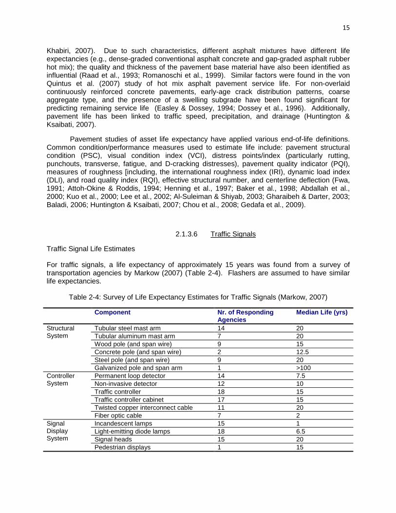
15
Khabiri, 2007). Due to such characteristics, different asphalt mixtures have different life expectancies (e.g., dense-graded conventional asphalt concrete and gap-graded asphalt rubber hot mix); the quality and thickness of the pavement base material have also been identified as influential (Raad et al., 1993; Romanoschi et al., 1999). Similar factors were found in the von Quintus et al. (2007) study of hot mix asphalt pavement service life. For non-overlaid continuously reinforced concrete pavements, early-age crack distribution patterns, coarse aggregate type, and the presence of a swelling subgrade have been found significant for predicting remaining service life (Easley & Dossey, 1994; Dossey et al., 1996). Additionally, pavement life has been linked to traffic speed, precipitation, and drainage (Huntington & Ksaibati, 2007).
Pavement studies of asset life expectancy have applied various end-of-life definitions. Common condition/performance measures used to estimate life include: pavement structural condition (PSC), visual condition index (VCI), distress points/index (particularly rutting, punchouts, transverse, fatigue, and D-cracking distresses), pavement quality indicator (PQI), measures of roughness [including, the international roughness index (IRI), dynamic load index (DLI), and road quality index (RQI), effective structural number, and centerline deflection (Fwa, 1991; Attoh-Okine & Roddis, 1994; Henning et al., 1997; Baker et al., 1998; Abdallah et al., 2000; Kuo et al., 2000; Lee et al., 2002; Al-Suleiman & Shiyab, 2003; Gharaibeh & Darter, 2003; Baladi, 2006; Huntington & Ksaibati, 2007; Chou et al., 2008; Gedafa et al., 2009).
2.1.3.6 Traffic Signals
Traffic Signal Life Estimates
For traffic signals, a life expectancy of approximately 15 years was found from a survey of transportation agencies by Markow (2007) (Table 2-4). Flashers are assumed to have similar life expectancies.
Table 2-4: Survey of Life Expectancy Estimates for Traffic Signals (Markow, 2007)
Component Nr. of Responding Agencies
Median Life (yrs)
Structural System
Tubular steel mast arm 14 20 Tubular aluminum mast arm 7 20 Wood pole (and span wire) 9 15 Concrete pole (and span wire) 2 12.5 Steel pole (and span wire) 9 20 Galvanized pole and span arm 1 >100
Controller System
Permanent loop detector 14 7.5 Non-invasive detector 12 10 Traffic controller 18 15 Traffic controller cabinet 17 15 Twisted copper interconnect cable 11 20 Fiber optic cable 7 2
Signal Display System
Incandescent lamps 15 1 Light-emitting diode lamps 18 6.5 Signal heads 15 20 Pedestrian displays 1 15

16
Review of Traffic Signal Life Expectancy Factors
Factors influencing traffic signal head life have been found to include: localized wind/gust strength, dominant wind direction with respect to the signal orientation, structure material type, type of structural connections, and climatic and weather factors (South, 1994; Chen et al., 2001; Kloos & Bugas-Schramm, 2005; Lucas & Cousins, 2005; Schrader & Bjorkman, 2006; Markow, 2007).
2.1.3.7 Roadway Lighting
Roadway Lighting Life Estimates
Markow (2007) surveyed agencies on roadway lighting structure life, and subsequently established typical estimates varying between 25 and 30 years (Table 2-5). As demonstrated later in the present NCHRP 08-71 study, far higher life estimates were found for roadway lighting structures, using historical data. The lower estimate from expert opinion is indicative of the need for recordkeeping and data analysis to replace expert opinion, or to revise expert opinion predictions.
Table 2-5: Survey of Life Expectancy Estimates for Roadway Lighting (Markow, 2007)
Component Nr. of Responding Agencies
Median Life (yrs)
Structural System
Tubular steel 12 25 Tubular aluminum 9 25 Cast metal 2 22.5 Wood posts 2 32.5 High mast or tower 11 30
Lamps Incandescent 3 1 Mercury vapor 6 4 High-pressure sodium 15 4 Low-pressure sodium 3 4 Metal halide 9 3 Fluorescent 1 5
Other Ballast 9 7.5 Photocells 11 5 Control panels 7 20 Luminaires 2 16.25
In addition to the surveyed agencies in Markow (2007), New Jersey and Ohio estimates lamp life at 2-5 years and 5-6 years, respectively (Zwahlen et al., 2003; Szary et al., 2005). In New Jersey, roadway lighting components have further been estimated to survive 8-10 years for batteries and 6-24 years for structural systems (Szary et al., 2005).
Roadway Lighting Life Expectancy Factors
Significant factors in roadway lighting life have included pole/bulb type, temperature extremes, and other environmental factors (Zwahlen et al., 2003; Szary et al., 2005).

17
2.1.4 Methods for Estimating Life Expectancy
Both empirical (statistical-evidence-based) and mechanistic (physical-based) models have been applied in the literature of life expectancy estimation. This report focuses on empirical models. However, for the sake of completeness of the information search, a brief review of mechanistic approaches is first provided.
2.1.4.1 Mechanistic Methods for Estimating Life Expectancy
Mechanistic methods generally involve the use of field or laboratory tests, which can be destructive or non-destructive, to measure a physical property such as corrosion, stress, or strain of an asset or component thereof. Theories regarding material behavior are then applied to extrapolate fatigue or physical life information. For concrete structures for example, mechanistic approaches and applications that have been used in past research for predicting the life of the asset or its structural components are described in Table 2-6.
Table 2-6: Mechanistic Methods for Predicting Concrete Structure Life (Liang et al., 2002)
Method Influence or Application References in (Liang et al., 2002)
Physical-mathematical model
Predicted time of tp and tcor Bazant (1979a,b)
Accelerated durability test method
Prediction of the service life of a structure depended on minimum load-carrying capacity, maximum acceptable deformation, and permeability
Fagerlund (1979)
Evaluation of parameters of deterioration
Use in formulating repair rehabilitation, replacement policy, underestimated value of tcor
Cady & Weyers (1984)
Accelerated test and mathematical model
Prediction of concrete service life Pommersheim & Clifton (1985)
Probabilistic view Prediction of service life of building materials and components
Sjostrom (1985)
Failure probability Design life and durability of concrete structures
Somerville (1986)
Survey data of bridge decks exposed to deicing salt, coastal buildings, and offshore structures
Predicted initiation time Guirguis (1987)
Systematic approach Service life prediction of building and construction materials
Masters (1987)
Unsteady-state dynamic analysis (using the semi-infinite solid approximation and the Laplace transform. method)
Service life prediction for external vertical walls of RC with external thermal insulations
Fukushima (1987)
Modified version of Bazant's model
Predicted time of tp Subramanian & Wheat (1989)

18
Table 2-6 Continued Method Influence or Application References
in (Liang et al., 2002)
Predictive service life test, aging test, and mathematical model
Service life prediction of building materials and components
Masters & Brandt (1989)
Experimental and field tests Prediction of corrosion depth in concrete Tsaur (1989)
Expanded and Bazant model Prediction of the tp time, the corrosion cracking time, the breaking time of bond between concrete and steel, and the steel area losing time
Liu & Mian (1990)
Allowable limit and the state of corrosion
Prediction of service lives of RC buildings, but the predicted results are always overestimated
Morinaga (1990)
Predictive service life tests and long term aging, and in-use conditions
Systematic methodology for the prediction of service life of building materials and components
Sjostrom & Brandt (1990)
Mathematical deterioration model expressed the property changing as a function of solar ultraviolet rays, heat, and degradation factors
Service life prediction system of building materials
Tomiita (1990)
Mathematical model consists of the assessment of the annual total damage ratio and the estimation of the service life
To estimate the service life of a bituminous glass-fibre-reinforced multiple waterproof roofing element
Ahoz & Akman (1990)
Probabilistic approach Service life prediction of ferrocement roof slabs
Quek et al. (1990)
Experience, deduction, accelerated testing, mathematical modeling, reliability, and stochastic concept
Predicting the service life of concrete Clifton (1990, 1991, 1993)
Measurement of the corrosion rate of reinforcing steel
Prediction of service lives of RC building Morinaga (1990)
Accelerated corrosion tests and field measurement
Measure the rate of steel corrosion in concrete
Harn et al. (1991)
Gray theory Predicts remaining service life of harbor structures
Li (1992)
Implementation of Tuntti's model [considers effect of temperature, chloride proportion, & humidity in concrete pores (resistivity)]
Influence of temperature on the service life of rebars
Lopez et al. (1993)
Time-dependent reliability Service life assessment of aging concrete structures
Mori & Ellingwood (1993)
Probability method Service life prediction of existing concrete bridges
Qu (1995)
Reliability approach Predicts service life of concrete structures exposed to chloride ions
Prezzi et al. (1996)
Fick's second law Predicts service life of existing concrete exposed to marine environments
Maage et al. (1996)
Testing, structural, and economic models
Service life of existing RC structures Henriksen (1996)

19
Table 2-6 Continued Method Influence or Application References in (Liang et
al., 2002) Generalization of Markov Chains based on time-dependent reliability theory
Prediction of bridge service life Ng and Moses (1996)
Long-term economic analysis Service life prediction of concrete road bridges
Brito & Branco (1996)
Calculation of prestressing cable forces from vibro-wire gauges embedded in bridges
Service life prediction of prestressed concrete cantilever bridge
Javor (1996)
Corrosion damage prediction using electrical potential surveys
Service life prediction of concrete bridge deck
Kriviak et al. (1996)
Utilization of measured stress spectra for predicting fatigue accumulation and crack propagation
Service life evaluation of steel or composite bridge; influence of the effective traffic loading on structures
Baumgartner et al. (1996)
Established a computer-integrated knowledge system
Predicting the service life of steel-RC exposed chloride ions
Bentz et al. (1996)
In situ permeability and strength testing Develop the durability-based design criteria for concrete and assess the remaining life of existing structures
Long & Rankin (1997)
Cumulative damage theory and accelerating the corrosion of rebar in concrete
Service life prediction of rebar-corroded RC structure
Ahmad et al. (1997)
Mathematical model for accelerated testing for concrete structures in chloride laden environments
Predicting the initiation time of concrete structures
Liang et al. (1997, 1999a)
Mathematical model combined Fick's second law with durability coefficient
Predicting the service life of existing RC bridges due to carbonation
Liang et al. (1998, 1999b)
Time-variant reliability method, Monte-Carlo simulation for finding the cumulative-time system failure probability
Service life prediction of deteriorating concrete bridges
Enright & Frangopol (1998)
Fick's second law incorporated surface environment, chloride transport, temperature of surrounding medium, seasonal effects, and construction variability
Predicting the service life of a RC structure in different environments
Amey et al. (1998)
FBECR (fusion-bonded epoxy-coated reinforcing steel) as a physical chloride barrier system
FBECR is not a cost-effective corrosion protection system when compared with bridge built with bare steel in Virginia, because they only provide corrosion protection for 5% of Virginia's bridge decks
Weyers et al. (1998)
Time-to-cracking model based on elasticity
Corrosion cracking model is dependent on the cover depth, properties of the concrete and steel/concrete interface, type of corrosion products, and the size of the reinforcing steel and is a function of the critical weight of rust products and corrosion rate
Weyers (1998), Liu & Weyers (1998)

20
Of the mechanistic-based methods in Table 2-6, service life is commonly predicted as a function of corrosion, particularly for assets, such as reinforced-concrete box culverts, that are susceptible to this mode of deterioration. Corrosion occurs in three stages (Liang et al., 2002):
1. Initiation time – The time for chloride ions to penetrate the concrete surface and onto the passive film surrounding the reinforcement;
2. Depassivation time – The time for the chlorides, transported to the steel by the alkaline hydrated cement matrix, to locally destroy the passive film leading to pitting corrosion; and
3. Propagation or corrosion time – The time when corrosion products form and cracking, spalling, or sufficient structural damage occurs.
Generally, the first two stages are modeled together and can jointly be considered as the initiation time. Attempts to model these time stages are shown in Table 2-7; the service life is then the sum of the two time periods.
Table 2-7: Prediction of Corrosion Time Stages (Liang, Lin, & Liang, 2002)
Time Prediction Method Formula
Reference in (Liang et al.,
2002)
Initiation Time, tp
Weyers ���, �� � �√� 1 � erf � �2������ Weyers (1998)
LZCL ���, �� � �� � ������ � ���erfc � �2���������
Liang et al. (2001)
Hookham
� � ��� �! � �"� Hookham (1992)
AJMF
���, �� � #� $�1 � �!2���� erfc � �2�����
� � ��%���� ��&'/)*+�, Amey et al. (1998) ���, �� � #√� $��&'/)*+�
� �√%�%���� erfc � �2�����,
Initiation Time, tp
Guirguis � � -.�� Guirguis (1987)
Bazant � � -12�� /0 -
1 � 1�2�345
!
Bazant (1979b)

21
Table 2-7: Continued
Time Prediction Method Formula
Reference in (Liang et al.,
2002)
Propagation time, tcor
Bazant ��67 � 8�67 �9 �2;7 , �2 � 2<=� -� >??
Bazant (1979b)
Modified Bazant ��67 � 8�67 �9 �2
;7 , Δ�2 � <=� @2 A-�B � 1C >?? Proposed
CW ��67 � 2~5 years Cady & Weyers (1984)
Liu
��67 � J�7��!2#?
J�7�� � 8�67 $% -<=�K L �M! � N!M! � N! � O�� � PQ� �
� J��8�� ,
#? � 0.098 1V %�W�677 , V � 0.57
Liu (1996)
Faraday’s Law
��67 � >8��YZ[W�677
Fontana (1987) Mangat & Elgarf (1999)
The more common techniques for predicting corrosion stage times is Fick’s law (Daigle et al., 2008) and the Weyers technique, as used in NCHRP Report 558 (Sohanghpurwala, 2006). To slow the ingress of chlorides in concrete structures, asset managers have used low-permeability concretes, polymer overlays, deck sealers, increased concrete cover depth, cathodic protection, and looked into alternative reinforcements (Kirkpatrick et al., 2002).
For steel structures, fatigue is more commonly used as a basis for estimating life. Previous experimental studies analyzing fatigue with accelerated loading have included the application of vibration theory, fatigue damage theory, fracture mechanics, the Palmgren-Miner linear damage equation, Miner’s hypothesis test, and finite element-based methods (Coetzee & Connor, 1990; South, 1994; Romanoschi et al., 1999; Lund & Alampalli, 2004; Breysse et al., 2005; Lu & de Boer, 2006; Lipkus & Brasic, 2007; Zuo et al., 2007; Samson & Marchand, 2008). One common method of assessing fatigue is the use of Miner’s Hypothesis [e.g., (Tanquist, 2002)]:
\ ]�̂� � ��
�_`
Where: n represents the accumulation of loads over cycle i, N represents the maximum allowable load cycles, and C represents the fractional life when C is assumed to be 1.

22
The fatigue life of steel bridges can also be calculated using the AASHTO Guide Specifications for Fatigue Evaluation of Existing Steel Bridges (AASHTO, 1990), which has been used to model the time until a failure mechanism occurs (Lund & Alampalli, 2004; Metzger & Huckelbridge Jr., 2006).
Another common technique in bridge life estimation is reliability analysis. This term is generally considered synonymous with the empirical techniques that involve survival analysis. However, in the bridge field, the term reliability pertains to some probabilistic, time-variant index based on the interplay between structural resistance (such as shear and moment strength, reinforcement strength, spacing, diffusivity), governed by the LRFD (AASHTO, 2010), on one hand, and demand (such as traffic volume or truck weights) on the other hand. The life of the asset is taken as the time until the index reaches a pre-specified target level. These indices can be applied to the overall structure or to multiple bridge components. Studies that examined bridge reliability, particularly with the incorporation of probabilistic material strengths, include Lin (1995), Deshmukh & Bernhardt (2000); Lounis (2000), Akgul & Frangopol (2004), Stewart et al. (2004), Biondini et al. (2006), Saber et al. (2006), Oh et al. (2007), and Strauss et al. (2008). Mechanistic models are typically calibrated using laboratory or field experiments under controlled and accelerated conditions that simulate the deterioration of long-lived assets [e.g., (Roesler et al., 1999)]. These tests, however, are limited to the accuracy of controlled representations of real-world conditions.
For purposes of asset management and network-level planning, empirical methodologies for life expectancy estimation can be considered more appropriate for the practice and consequently remained the focus of the investigation.
2.1.4.2 Empirical Methods for Estimating Life Expectancy
Empirical modeling techniques for estimating life either directly or via deterioration levels fall into four categories. Past studies that have utilized these categories for estimating asset life, as herein listed:
• Statistical regression o Bridges: Polynomial functional form (Agrawal & Kawaguchi, 2009); o Culverts: Linear, log-linear, and exponential functional forms (Hadiprono et al.,
1988; Kurdziel & Bealey, 1990; Halmen et al., 2008); o Traffic Signs: Linear, power, exponential, and power functional forms (Kirk et al.,
2001; Bischoff & Bullock, 2002; Immaneni et al., 2009); o Pavement Markings: Exponential and smoothing spline functional forms (Abboud
& Bowman, 2002; Zhang & Wu, 2006); o Pavements: Linear, polynomial, exponential, log-linear, power, and sigmoidal
functional forms: (Labi, 2001; Lee et al., 2002; McManus & Metcalf, 2003; Flom & Darter, 2005; Yu, 2005; Chou et al., 2008; Gedafa et al., 2009);
o Roadway Lighting: Exponential functional form (Szary et al., 2005). • Markov chains
o Bridges: (Jiang & Sinha, 1989; Ng & Moses, 1996; Estes & Frangopol, 2001; Zhang et al., 2003; Hallberg, 2005; Morcous, 2006; Ertekin et al., 2008; Robelin & Madanat, 2008);
o Pavements: (Chou et al., 2008). • Duration models

23
o Bridges: Weibull, Exponential, Rayleigh, and Gamma survival models (Ng & Moses, 1996; Klatter & Van Noortwijk, 2003; van Noortwijk & Klatter, 2004; Hearn & Xi, 2007; Nicolai, 2008; Agrawal & Kawaguchi, 2009);
o Pavement Markings: Weibull survival models (Sathyanarayanan et al., 2008); o Pavements: Kaplan-Meier estimate, Cox proportional hazards model, and normal,
lognormal, exponential, log-logistic, and Weibull survival distributions (Vepa et al., 1996; Colucci et al., 1997; Eltahan et al., 1999; Romanoschi et al., 1999; Shekharan & Ostrom, 2002; Gharaibeh & Darter, 2003; Bausano et al., 2004; Yu, 2005; Yang, 2007; Yu et al., 2008; Anastasopoulos, 2009; Irfan et al., 2009);
o Culverts: Normal and Weibull survival distributions (Halmen et al., 2008; Meegoda et al., 2008);
o Roadway Lighting: Kaplan-Meier estimate (Zwahlen et al., 2003). • Machine learning
o Bridges: k-nearest neighbor inference based learning, inductive learning, and artificial neural networks (Melhem & Cheng, 2003; Narasinghe et al., 2006);
o Traffic Signs: Artificial neural network (Swargam, 2004); o Pavements: Artificial neural network (Flintsch et al., 1997; Ferregut et al., 1999;
Abdallah et al., 2000). Generally, it was found that statistical regression has most commonly been applied for the prediction of performance for less-costly assets such as traffic signs, pavement markings, and pipe culverts. Markov chains have been mostly limited to pavements and bridges, likely because their calibration requires extensive inspection ratings. Various survival models have been applied to explain pavement service life while structural reliability analysis has been more commonly used for predicting bridge life. Of the survival models, the Weibull distribution is widely used across all asset classes. Machine learning has been applied primarily to bridges and pavements, but to a lesser extent than the other approaches, likely due to such estimates being considered to come from a ‘black box’. A more extensive treatment on the theory of the probabilistic approaches is provided in Section 2.2.4.
2.2 Methodology for Estimating Asset Life
In building on the literature, one of the goals of this study was to develop an overarching methodology that could be applied for a variety of asset classes in order to predict highway asset life expectancy. For the methodology used in this study (Figure 2-5), each step is discussed in subsequent subsections.
Figure 2-5: General Methodology for Estimating Highway Asset Life Expectancy
Identify Replacment
Rationale
Define End-of-Life
Select General
Approach
Select Modeling Technique
Fit Model to Data

24
2.2.1 Identify Replacement Rationale
The first step in the developed methodology for predicting asset life expectancy is to identify the rationale for the asset replacement. As discussed in a previous section of this report, such rationale may generally include: structural adequacy and safety, serviceability and functional obsolescence, essentiality for public use, and special reductions. For competing rationales, multiple life estimates can be established for purposes of comparison.
2.2.2 Define End-of-Life
On the basis of the selected rationale, the next step is to select a representative condition or performance measure that is pertinent to the asset replacement rationale under consideration. For bridge assets for example, structural adequacy and safety can be represented by the superstructure, substructure, channel, and scour condition ratings; serviceability and functional obsolescence can be represented by the deck condition rating and deck geometry rating; essentiality for public use can be represented by ADT; and special reductions can be evaluated based on annual maintenance costs. Given a quantitative measure of the rationale, a minimum acceptable threshold, or trigger, is needed. This threshold typically is chosen to reflect the point at which intermediate maintenance actions are no longer cost effective [e.g., (Saito & Sinha, 1989)].
2.2.3 Select General Approach
Three general life estimation approaches that are common in the literature are: (1) condition-based approach, and (2) age-based approach. For each of these two approaches, the data used could be from expert opinion surveys or data from in-service assets. Generally, it can be found that lesser studied asset life expectancies are determined based on expert opinion or manufacturer published values. These values are then commonly used to conduct blanket replacements. This strategy, however, puts agencies at risk for either foregoing remaining service life or allowing an asset to operate at unacceptable level of service.
2.2.3.1 Condition-based Approach
The condition-based approach has been commonly used for estimating the service life or physical life of higher-valued assets (i.e., bridges and pavements). These assets are periodically monitored/inspected with respect to their condition. As such, deterioration models can be readily developed. The life expectancy is then taken as the time from construction or last reconstruction until one or more performance measures trigger replacement. For instance, if an agency sets a minimum performance threshold for a pavement’s level of cracking or rutting, then the time when the threshold is first crossed (Figure 2-6).
Such condition-based life estimates could also be viewed with respect to the occurrence of an extreme event [e.g., (Sanchez-Silva & Rosowsky, 2008)].
The selection of the performance measure can vary based on the rationale for replacement to be considered. If replacement is being considered due to structural adequacy and safety, then for pavements an agency may wish to predict rutting, PCR, percent cracks; for bridges, predictions of discrete NBI ratings for decks, substructures, superstructures, structural evaluation, and scour can be made; for other assets, some visual rating of condition can be predicted. If replacement is being considered due to serviceability or functional obsolescence, then pavements can be modeled to predict IRI or PSR; for bridges, the NBI deck geometry or

25
waterway adequacy could be predicted; for culverts, percent blockage or channel erosion can be considered; for traffic signs and pavement markings, retroreflectivity can be measured; for traffic signals and roadway lighting, luminescence may be predicted. If ‘essentiality for public use’ requires replacement, then economic development considerations may be used. This could be modeled based on traffic forecasts. For special reductions, performance could be based on annual maintenance costs to keep the asset in a serviceable state. Multiple rationale can be considered within one prediction as well. For example, the NBI sufficiency rating for bridges consider all of the above mentioned replacement rationale. If one combined factor has not been agreed upon by an agency, then the minimum of a series of life values may be taken.
Figure 2-6: Condition-based life expectancy (Conceptual Illustration) (Thompson et al., 2011)
2.2.3.2 Age-based Approach
In the age-based approach, historical replacement records regarding the year of construction and year of demolition/reconstruction are assessed (Figure 2-7). The actual life is best quantified using this approach. In this approach, the asset life can be directly predicted and easily incorporated into replacement scheduling decisions.
Figure 2-7: Age-based life expectancy (Conceptual Illustration)
The accuracy of age-based predictions are highly dependent on data availability and
integrity. Many agencies lack complete historical records relating to the year built, maintenance strategies, traffic volumes, etc. Without sufficient archived information, the credibility of results may be brought into question. A key piece of information not available in the collected dataset for this study, was the rationale or motive behind the replacement of the assets considered. With such data, agencies could organize calibration datasets for only those rationales that are considered relevant. For instance, if bridge widening is no longer considered necessary, then agencies need only analyze the observed lifespan for alternative bridge replacement rationale. More generally, this approach assumes that the future will mimic the past which could be invalid
Service Life 1 Service Life 2
Time, t Construction Reconstruction 1 Reconstruction 2

26
in light of emerging materials, construction processes, contracting approaches, climate change, etc.
2.2.3.3 Condition/Age-based Hybrid Approach
Combining the two approaches may also be preferred, so as to directly make life predictions based on condition. For instance, the time until an inadequate sufficiency rating is obtained for a bridge can be predicted, as opposed to predicting sufficiency rating by age. Combining historical replacement records and observed times until a condition/performance threshold is reached can also be applied.
2.2.4 Select Modeling Technique
In selecting a modeling technique, agencies should consider three dimensions of analysis: the first dimension relates to the basic asset attributes (e.g., asset class, design/material type); the second dimension relates to the nature of the data (such as, if the data is cross-sectional, time-series or panel; if the dependent variable is discrete or continuous; if sufficient condition-based, age-based, or hybrid model data is available; geographic representation of the data; and if explanatory variables are available to be analyzed); and the third attribute relates to the modeling techniques (such as, if a deterministic or probabilistic model is preferred; the specific statistical technique that is to be used; and the measure of goodness-of-fit used to validate model results).
On the basis of the selections made at each level, different approaches in the following dimensions may be recommended. For instance, if the asset manager seeks to predict the service life of a steel box culvert (1st level), then a condition-based approach to predict a discrete visual condition rating may be applied given the lack of historical replacement data (2nd level), which would then suggest that a discrete choice model or Markov chain may be the most appropriate (3rd level).
Modeling can be used to avoid the inherent errors in assuming or transferring a life expectancy value that may not be representative of local conditions. In doing so, statistical evidence can be obtained using local data, as well as the additional benefit of identifying influential factors and assessing their sensitivity. In order to facilitate uncertainty analysis, probabilistic, empirical modeling techniques are recommended. However, agencies are recommended to select a modeling techniques based on the nature of the response or dependent variable and staff expertise. From the literature review and research team knowledge, six modeling techniques were identified for potential application:
• Linear and Non-linear Regression Models – continuous, deterministic model type with direct interpretations of model fit (R2) and parameter strength.
• Neural Networks – continuous, deterministic model type that relies on hidden relationships between sets of variables in order to make forecasts, but is often viewed as a ‘black box’.
• Discrete Outcome Models – discrete, probabilistic, and parametric model type that can be applied to ordered data to predict condition states.
• Markov Chains – discrete, probabilistic, and non-parametric model type that can predict the probability of being in any discrete state at any point in time.
• Duration Models – continuous, probabilistic model type that produces non-, semi-, or fully-parametric survival curves and allows for capturing covariate influences.
• Markov-based Duration Models – fits a continuous, probabilistic, fully-parametric survival curve to a Markov Chain estimate.

27
In choosing between the modeling techniques, agencies should consider the availability of data. Without a measure of condition/performance, duration models can be calibrated to observed, historical service life. When discrete condition/performance measures are routinely collected as part of an inspection, Markov-based models can be calibrated. When the data is not routinely collected or is of a continuous nature, a duration model can be fit to the time at which the threshold value is crossed.
A brief review of such model types is provided in the following subsections.
2.2.4.1 Regression Models
Linear and non-linear regression models are the most commonly applied by agencies due to their simplicity, clarity of results, and ability to be calibrated with widely available software such as MS Excel. Such models can be applied to predict a continuous performance measure (condition-based) as a function of age and other variables, or to directly predict service life as a function of explanatory variables (age-based). Latent variable and adaptive approaches can also be examined; that is, predict condition as a function of past performance and characteristics. Discrete/continuous models can also be estimated using a system of linear equations. Various model functional forms and types can be applied, including:
Polynomial
a � bQ � \ b���c�_`
If n =1, then Linear If n =2, then Quadratic If n =3, then Cubic Exponential/Logistic
a � dbQ � \ V�b�&ec
�_`f� for k � �1 or 1
If k = 1, then Exponential If k = –1, then Logistic Gompertz
a � \ i�V�jekec�_`
Where: Y represents a dependent variable ci, αi, and βi represent estimable parameters and xi represents an independent variable
For linear models, various model subtypes can be calibrated, including: ordinary, indirect, generalized, two-stage, and three-stage least squares, instrumental variables, limited and full information maximum likelihood, and seemingly unrelated regression. The most efficient and consistent of these models are the system equation methods commonly applied for simultaneous equations, as opposed to single equation methods: [i.e., ordinary least squares

(OLS), indirect least squares (ILS), instrumental variables (IV), twoand limited information maximum likelistage least squares (3SLS), seemingly unrelated regression estimation (SURE), and full information maximum likelihood (FIML). Such models are better suited for dealing with serial correlation problems (i.e., lack of independence among explanatory variables), heteroskedasticity (i.e., variables with noncreated by endogenous variables (i.e., variables where there is not a unidirectional causal relationship from the independent variable to the dependent variable)
In 3SLS, least squares regression is performed in three stages: (1) get 2SLS estimates of the model system, (2) use the 2SLS estimates to compute residuals to determiequation correlations, and (3) use generalized least squares (GLS) to estimate model parameters as similarly done in SURE multiple rounds of OLS to predict instrumentto be endogenous) which in turn predict the dependent variable. This process results in a more efficient and consistent linear regression model.
Of this set of model subtypes, the 3SLS approach is recommended. For panel datrandom effects can be added to account for correlation (e.g., multiple inspections for a single structure).
Despite their simplicity innumber of disadvantages for this general model type. Linear regression methods are only appropriate when the dependent variable has a linear explanatory variables, which may not necessarily be the case for highway asset performance behavior over time. Furthermore, such models are deterministicestimate that may not reflect the true On the other hands, for non-linear models, it is significant independent variablesdetermination (R2), they typically lack explanatory power due to thesignificant variables.
A second approach to consider is that of artificial neural networks. This nonmodel predicts conditions based on what it has ‘learned’ (pattern identification) from past data. Statistically, an artificial neural network is a nonpredicted to predict future events
Figure 2-8
(OLS), indirect least squares (ILS), instrumental variables (IV), two-stage least squares (2SLS), and limited information maximum likelihood (LIML)]. System equation methods include threestage least squares (3SLS), seemingly unrelated regression estimation (SURE), and full information maximum likelihood (FIML). Such models are better suited for dealing with serial
i.e., lack of independence among explanatory variables), heteroskedasticity (i.e., variables with non-constant standard deviations), and mitigating errors created by endogenous variables (i.e., variables where there is not a unidirectional causal
hip from the independent variable to the dependent variable) (Washington et al., 2003)
In 3SLS, least squares regression is performed in three stages: (1) get 2SLS estimates of the model system, (2) use the 2SLS estimates to compute residuals to determiequation correlations, and (3) use generalized least squares (GLS) to estimate model parameters as similarly done in SURE (Washington et al., 2003). In other words, multiple rounds of OLS to predict instrumental variables (that is, variables that are “suspected”
endogenous) which in turn predict the dependent variable. This process results in a more efficient and consistent linear regression model.
Of this set of model subtypes, the 3SLS approach is recommended. For panel datrandom effects can be added to account for correlation (e.g., multiple inspections for a single
in interpretation (particularly for linear regression), there this general model type. Linear regression methods are only
appropriate when the dependent variable has a linear or intrinsically linear relationship with the may not necessarily be the case for highway asset performance
Furthermore, such models are deterministic, and thus yield not reflect the true value of condition or service life that could be expected
linear models, it is generally far more difficult to develop a set of significant independent variables; while these models may yield higher coefficients of
), they typically lack explanatory power due to their composition
2.2.4.2 Neural Networks
pproach to consider is that of artificial neural networks. This nonmodel predicts conditions based on what it has ‘learned’ (pattern identification) from past data. Statistically, an artificial neural network is a non-linear form of 3SLS, where instruments are predicted to predict future events (Figure 2-8).
8: Example of an Artificial Neural Network
28
stage least squares (2SLS), . System equation methods include three-
stage least squares (3SLS), seemingly unrelated regression estimation (SURE), and full information maximum likelihood (FIML). Such models are better suited for dealing with serial
i.e., lack of independence among explanatory variables), constant standard deviations), and mitigating errors
created by endogenous variables (i.e., variables where there is not a unidirectional causal (Washington et al., 2003).
In 3SLS, least squares regression is performed in three stages: (1) get 2SLS estimates of the model system, (2) use the 2SLS estimates to compute residuals to determine cross-equation correlations, and (3) use generalized least squares (GLS) to estimate model
In other words, 3SLS relies on variables that are “suspected”
endogenous) which in turn predict the dependent variable. This process results in a more
Of this set of model subtypes, the 3SLS approach is recommended. For panel data, random effects can be added to account for correlation (e.g., multiple inspections for a single
(particularly for linear regression), there exist a this general model type. Linear regression methods are only
relationship with the may not necessarily be the case for highway asset performance
and thus yield only a point value of condition or service life that could be expected.
fficult to develop a set of higher coefficients of
ir composition of fewer
pproach to consider is that of artificial neural networks. This non-linear, adaptive model predicts conditions based on what it has ‘learned’ (pattern identification) from past data.
S, where instruments are

29
To facilitate learning, such models are typically Bayesian-based. This approach updates estimates (i.e., posterior means) by applying weighted averages based on previous estimates (i.e., prior means). Typically, these weights are based on the number of observations. Activation functions within the network have included hyperbolic tangent, log-sigmoid, and bipolar-sigmoid functions. Such approaches have been found to work well with noisy data and are relatively quick; however, such techniques are better suited for smaller databases (Melhem & Cheng, 2003). These models require more sophisticated software to develop (e.g., Palisade’s @Risk Neural Tools, NeuroXL) and can sometimes be used as a ‘black box’ (i.e., prediction process unknown but assumed appropriate). However, the ability to ‘learn’ makes these models particularly useful to asset managers.
2.2.4.3 Ordered Discrete Response Models
Given the use of discrete condition ratings and functional classifications, it is considered more appropriate to apply discrete outcome models. Based on an assumed distribution, these models can be used to calculate the probability of an asset being in any condition state. For instance, the probability of a bridge being in any condition state of the NBI rating scale (0-worst to 9-best) in any future year can be calculated using these models. Such models also simplify sensitivity analysis, through the analysis of marginal effects (i.e., how probability of a condition state changes given a unit change in one of the inputs), and can be used for panel, ordered, and/or nested data.
Model subtypes are typically of the probit or logit form, and can be modified as follows:
• ordered (e.g., NBI condition rating) or unordered (e.g., bridge status – functionally obsolete, structurally deficient, satisfactory condition),
• nested (e.g., predict status of all concretes bridge at first level, then predict status of pre-tensioned concrete bridges and post-tensioned concrete bridges at the second nest level), or
• incorporate mixed, fixed, or random effects (to account for asset heterogeneity) for panel data.
Probit models assume normally distributed variates, whereas logit models assume extreme value distributions. Depending on the data, similar results may be obtained.
Probit
l�a�� � m Ab���c � b�n`���n`�co B � 1√2% p Kql A� 12 r!B Prje&es�jetu&�etu�sv�∞
Logit
l�a�� � Kql �b����∑ Kql �b����c�_`
For ordered models, threshold parameters are calibrated to indicate the probability of a condition state. For example, the probability that an asset is in any of three condition states can be computed from an ordered probit model by comparing the model sum (∑ b�) to the threshold parameters (µ) (Figure 2-9). Mathematically, the exact probability of such an asset being in any condition state follows the cumulative standard normal distribution with the variable X taking the following forms:

30
l��x]PW�Wx] ��M�� � 0� � y� \ b�z ~^�0,1�
l��x]PW�Wx] ��M�� � 1� � y{` � \ b�z ~^�0,1� � y� \ b�z ~^�0,1�
l��x]PW�Wx] ��M�� � 2� � y{! � \ b�z ~^�0,1� � y{` � \ b�z ~^�0,1�
l��x]PW�Wx] ��M�� � 3� � 1 � y{! � \ b�z ~^�0,1�
Where: x represents the set of independent variables, age, material type, etc.; β represents the set of parameter estimates; µ represents the threshold parameters, which in comparison to parameter estimates and variable values, indicate the likelihood of being in a given condition state: X = [µ - ∑ β x] and Y � }�~ "c3�"c�"7� * ��"��6c
N(0,1) represents the cumulative standard normal distribution with mean = 0 and standard deviation = 1
Figure 2-9: Example illustration of a 3-state ordered probit model (Washington et al., 2003)
These models, however, are only appropriate if the assumed distribution accurately reflects the data. Furthermore, with discrete models in general there is a potential for aggregation bias. That is, two culverts may each have a condition rating of say 4 but one may
P(CR=1) P(CR=2) P(CR=3)
P(CR=0)
{` � \ b� � \ b� {! � \ b�

31
be nearly in a condition state of rating 3 while the other is nearly in a condition state of rating 5. This loss of generality may cause some errors in model calibration.
2.2.4.4 Markov Chains
Markov chains are commonly applied for estimating bridge deterioration curves. A Markov chain is a memoryless (i.e., transition probability based solely on the present state and not on past states), stochastic process with a finite, integer number of possible, non-negative states, that is used to predict the probability of being in any state after a period of time. These chains are commonly visualized in terms of a ‘graph’ showing all of the nodes (e.g., condition states) and possible paths (i.e., transitions). Calculations, based on the graph, are carried out using via matrix multiplication (Figure 2-10).
Markov Transition Matrix
State Today State Probability in One Year
Good Fair Poor
Good 95.3 4.6 0.1
Fair 0 93.2 3.9
Poor 0 0 100.0
Figure 2-10: Example Markov Chain Graph and Transition Matrix
The transition matrix corresponds to the probability of transitioning after a period of time (with discrete or continuous time intervals), which can be taken on an annual basis or based on inspection frequencies. When modeling deterioration, transitions to an improved state are considered impossible and assigned a transition probability of zero; likewise transitioning to a non-subsequent state may be assigned zero probability by some agencies.
Transition probabilities, represented by, ��� � Pr�Y�n` � j|Y� � i�, can be found via expert opinion, optimization (Jiang & Sinha, 1989), statistical modeling, simulation (Robelin & Madanat, 2008), based on observed frequencies (methodology used in this study), or approximated using pairs of inspections (Thompson et al., 2011). To correct for the fact that deterioration rates are not homogenous throughout the life of an asset, multiple transition matrices are typically established for several age ranges [e.g., (Jiang & Sinha, 1989)]. Also,
Good Fair Poor
P GG=95.3
P GF=4.6
PGP =0.1
P FF=93.2 PPP =100.0
PFP =3.9

32
Bayesian techniques could be used to update transition probabilities as well. Predictions at various points in time can be derived from the Chapman-Kolmogorov equation [e.g., (Weisstein)] to yield:
���� � ����� � l�c�
Where: p(ti) represents the initial state, i, probability vector (e.g., [1, 0, 0] for a new traffic sign on a ‘good’, ‘fair’, ‘poor’ rating system starting at time 0); P represents the transition matrix; n represents the size of the age group interval.
2.2.4.5 Duration Models
Duration (sometimes labeled as reliability or survival) analysis is a probabilistic approach for predicting the likelihood of a continuous dependent variable passing beyond or ‘surviving’ at any given unit of time. The survival curve is just one representation of probability which can be applied to asset life (Table 2-8).
Table 2-8: Representations of Probability
Representation Relationship Life Expectancy Interpretation
Density Function <��� � PZ���P� Area under the curve represents the
probability between two life values
Cumulative Function Z��� � \ <�����e�� ‘Failure’ probability at any point in time
Survival Function ���� � 1 � Z��� Probability of surviving beyond any point in
time
Hazard Function ���� � <������� ‘Failure’ rate which is inversely related to
survival
As shown in Figure 2-11, survival curves can be produced for multiple performance measures or replacement rationale. The leftmost curves are the stochastically dominating functions in a life prediction.
Duration models can be non-parametric, semi-parametric, or fully-parametric. Non-parametric methods (e.g., Kaplan-Meier/product-limit estimator or life tables) are less commonly applied in transportation (more common in medical fields) because they do not retain the parametric assumption of the covariate influence; however they may be appropriate when there is little knowledge of the functional form of the hazard or if a small number of observations is obtained (Washington et al., 2003). The most common non-parametric estimator is the Kaplan-Meier estimate:
���� � � ]� � P�P��e��
Where: n represents the number of assets available at the start of the time period less censored cases (such as, assets that have left the analysis without a conclusive end value); d represents the number of assets ‘failed’ by the end of the time period.

33
Figure 2-11: Asset Survival Curves using Different Performance Indicators and Performance Thresholds (Irfan et al., 2009)
For the lower (L) and upper (U) bounds of a desired confidence level for a non-parametric model, such as the Kaplan-Meier, the following equations are recommended (Newcombe, 1998):
- � 2]� � �! � 1 � �1�! � 2 � 1] � 4��]� � 1�2�] � �!�
� � 2]� � �! � 1 � �1�! � 2 � 1] � 4��]� � 1�2�] � �!�
Where: n is the number of observations; p is the point estimate of probability (i.e., S(t) for Kaplan-Meier); q is taken as 1-p; z is the Normal distribution test statistic at the desired confidence level.
Semi-parametric models (e.g., Cox proportional-hazards), which account for covariate influence and are appropriate when the underlying distribution of the data is unknown, are considered more flexible without the constraint of a fully parametric form. The Cox model approach takes the following form:

34
���� � ����� 2 Kql dbQ � \ b���c
�_`f
Where: ����� represents a fully parametric, survival curve.
Fully-parametric models (e.g., gamma, exponential/Markov, Weibull, log-logistic, log-normal, Gompertz), are generally recommended in studies of this nature due to the benefits in model efficiency and in reducing bias, but they are influenced by the extent to which the assigned distribution fits the data. As found in the literature review, the Weibull survival curve is one of the most commonly applied distributions [e.g., (van Noortwijk & Klatter, 2004)]:
���� � Kql �1 2 A� � �V Bj� Where: α represents the scaling factor (stretches curve laterally); β represents the shape factor
(stretches curve vertically); γ represents the location factor (shifts curve horizontally by representing value at which 100% survival probability occurs).
The Weibull distribution is a more generalized form of the exponential distribution (β=1) that allows for a more flexible means of capturing duration dependence. Explanatory factors can also be incorporated to develop a fully-parametric survival curves with V � Kql�bQ �∑ b���c�_` �. The hazard function of the Weibull distribution is monotonic, indicating that the hazard never decreases over time (if β>1).
For distributions with non-monotonic hazard functions, log-logistic models can be applied (Washington et al., 2003). The model form for this distribution is:
���� � 1 � 1 � A b� � �B���`
A difficulty arises, however, when the location factor is effectively changing throughout the life of an asset. Just varying the location factor does not account for the changing hazard rate associated with the parametric specification (Ng & Moses, 1996). As such, the survival probability of in-service structures can be updated using conditional probability (Bayesian) theory:
���|� � �� � ��� � � � ������ � ��������
Where: T represents the age an asset is known to have survived.
To compare distributions, chi-squared test statistics can be computed based on the family of the distribution. The test statistic for functions in the same family can be approximated by (Washington et al., 2003):
�! � �2�--�b�� � --�b��� Where: χ2 represents the chi-squared test statistic; LL(βA,B) represents the log-likelihood of
distributions A and B (e.g., Exponential and Weibull distributions).

35
In the special case of the Exponential and Weibull distributions, a second technique is to calculate a modified t-statistic, which compares how significantly different the shape factors are.
�xPW<W�P � � 9�M�W9�Wi � b � 1�K
Where: β represents the parameter estimate; SE represents the standard error.
If the shape factor is significantly different from 1, then the Weibull distribution may be considered justified, else the Exponential distribution may be considered a better fit.
When comparing distributions from alternative families, an individual chi-squared test statistic should be calculated for each distribution (Washington et al., 2003):
�! � �2�--�0� � --�b��� Where: LL(0) represents the restricted log-likelihood function; LL(βC) represents the log-
likelihood function at convergence.
Using these test statistics, the Gamma, Weibull, Gompertz, Exponential, Log-Logistic, F, and Lognormal parametric duration models were tested in this study.
Finally, to validate the use of a distribution, the Kaplan-Meier survival curve can be compared to the baseline ancillary survival factors.
A further consideration in calibrating duration models, is the inclusion of censored data (Figure 2-12).
Figure 2-12: Censoring Types in Duration Modeling (Washington et al., 2003)
Data can be either left-censored, right-censored, both left and right censored, not captured, or completely captured over the period of observation. From interpreting Figure 2-12 in terms of asset life expectancies, the censored data types are: left-censored data (i.e., t4) indicate that the actual initial construction or reconstruction year is not observed but the time of replacement is; right-censored data (i.e., t5) indicate that the asset construction year is known but it has not been replaced during the time of observation; both types of censoring represent data (i.e., t2) where neither the construction/reconstruction year and year of replacement is observed; data not captured (i.e., t1) are those in which neither construction or replacement data is available;
Observation 1
Time a b
t1
t2
t3
t4 t5
Observational Period
(period for which data are available)
Observation 5
Observation 3
Observation 4
Observation 2

36
and the completely captured data would represent those assets for which knowledge of both the years of construction and replacement are known (i.e., t3).
Censored data can be problematic in that they can lead to more biased estimates, yet helpful in modifying predictions to account for observations that may have dissimilar properties from uncensored data. When more than half of a dataset is censored, the observed average time to failure is no longer predicted by the model and tail probability estimates are inaccurate (Kim, 1999; Ho & Silva, 2006). To help control bias from censoring, parametric models, or Bayesian inference when the distribution is unknown, are recommended (Kim, 1999). However, when dealing with long-term assets, such as infrastructure, right censored observations are particularly important to account for more modern designs (Klatter & Van Noortwijk, 2003). Such designs are less likely to have failed within the observational period, resulting in a prediction that does not capture the life expectancies of improved designs. Therefore, in this study, a 50/50 censoring split is assumed appropriate for predicting asset life.
2.2.4.6 Markov-based Duration Models
Markov-based duration models are a technique for fitting a parametric model estimate to a non-homogenous Markov chain with an absorbing state. In doing so, a parametric form, known to better represent life, can be calibrated to readily available inspection data and ease the correlated simulation required in uncertainty analysis. In this sense, the Markovian survival curve is analogous to the Kaplan-Meier estimate with probabilities found via matrix multiplication. That is, the Kaplan-Meier estimate is essentially a binary Markov chain with possible states being ‘failed’ or ‘survived’ (Hosgood, 2002). As such, the goal of fitting a parametric model (or multiple parametric models for intermediate transitions) is to minimize the difference to the non-parametric survival function (Perez-Ocon et al., 2001).
Homogenous Markovian probabilities are inherently exponentially distributed (multiplying by one transition matrix n number of times). However, if the duration in each state is non-exponential and data for a duration model is unavailable, then an alternative is needed. While, this may be sufficiently mitigated by using multiple transition matrices (i.e., piecewise exponential distributions), another technique is to fit a parametric survival curve to the Markovian survival curve.
Semi-Markov processes, commonly applied in power system analysis, have been used to convert back and forth between Markov chain models and generalized survival (typically Weibull) functions (Ng & Moses, 1996; van Casteren, 2001; Thompson et al., 2011). One such technique for this conversion, is the equivalent age technique, shown for a Markov/Weibull model (Thompson et al., 2011):
i. Estimate Markov transition matrix ii. Convert each row of the matrix to a median transition time
�� � �x��0.5��x�����
iii. Allocate a portion of asset life to each condition state, in proportion to transition time, to develop weights
r� � 1∑ ��� \ ��¡
�_�

37
iv. Compute a condition index using Markov predictions and weights which in turn approximates the Weibull survival probability �¢ � \ r����
v. Use the inverse of the Weibull survival model to calculate equivalent age
� � V 2 ���]��¢��j̀ vi. Optimize to maximize goodness-of-fit between the actual age corresponding to the
Markov prediction and the equivalent age Maximize ^x£¤M� -x� -W#��W�xxP� �0.5 2 �]�2%� � 0.5 2 �]�o!� � 0.5
2 ∑ �[�� x< �M£#xO l£�PWi�Wx]� � K�¥WOM��]� [���!c� o!
Subject to �M£#xO ��PWM] -W<� � ¢]O�£9� J�WN¥�� ��PWM] -W<�
b � 1 �M99¥¤W]� W]i£�M9W]�, ¤x]x�x]Wi �M�M£P�
By changing o, V, b This technique, however is more commonly applied when dealing with a time-homogenous Markov chain. For non-homogenous Markov chains, this study recommends an alternative approach that minimizes the root mean square error (RMSE) between the Weibull survival function and Markov chain survival curve by changing the Weibull scaling and shape factors, while maintaining the median life prediction. Markov/Weibull models are particularly useful for infrastructure where deterioration is initially slow and then accelerates with time.
For in-service assets, the same techniques can be applied to calibrate Markov/Beta models. The use of a Beta distribution has been recommended in past research for estimating remaining asset life (Li & Sinha, 2004) due to its flexibility in accounting for various hazard rates (e.g., change in hazard rate due to maintenance activity). The survival function of the Beta distribution is represented by:
���� � 1 � ¦ �§u¨u�`���§'¨u��©¨ª«ª¬¨ª« ¦ �§u¨u�`���§'¨u��u , V`, V! � 0
Where: �® represents the lower bound location factor; �¯ represents the upper bound location factor; V`, V! represent non-negative shape factors.
Advantages of Markov-based models include a probabilistic estimate, sole dependence on current conditions (i.e., minimal data needs if transition probabilities known), flexibility in modifying state duration, and efficiency for dealing with larger networks; disadvantages include the discrete nature, deterioration of components are described in visual terms only, assumption of constant inspection periods, lack of consideration of system condition, and independence from past data (if a first order Markov-chain is used) (Morcous, 2006; van Noortwijk & Frangopol, 2004). To overcome the assumption of constant inspection periods, Bayesian techniques can be applied (Morcous, 2006).
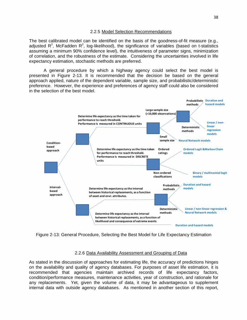
38
2.2.5 Model Selection Recommendations
The best calibrated model can be identified on the basis of the goodness-of-fit measure (e.g., adjusted R2, McFadden R2, log-likelihood), the significance of variables (based on t-statistics assuming a minimum 90% confidence level), the intuitiveness of parameter signs, minimization of correlation, and the robustness of the estimate. Considering the uncertainties involved in life expectancy estimation, stochastic methods are preferred.
A general procedure by which a highway agency could select the best model is presented in Figure 2-13. It is recommended that the decision be based on the general approach applied, nature of the dependent variable, sample size, and probabilistic/deterministic preference. However, the experience and preferences of agency staff could also be considered in the selection of the best model.
Figure 2-13: General Procedure, Selecting the Best Model for Life Expectancy Estimation
2.2.6 Data Availability Assessment and Grouping of Data
As stated in the discussion of approaches for estimating life, the accuracy of predictions hinges on the availability and quality of agency databases. For purposes of asset life estimation, it is recommended that agencies maintain archived records of life expectancy factors, condition/performance measures, maintenance activities, year of construction, and rationale for any replacements. Yet, given the volume of data, it may be advantageous to supplement internal data with outside agency databases. As mentioned in another section of this report,
Condition-
based
approach
Interval-
based
approach
Determine life expectancy as the time taken for
performance to reach threshold.
Performance is measured in CONTINUOUS units
Determine life expectancy as the interval
between historical replacements, as a function
of asset and envr. attributes.
Linear / non-
linear
regression
models
Large sample size
(>10,000 observations)
Small
sample size Neural Network models
Duration and
hazard modelsProbabilistic
methods
Deterministic
methods
Ordered
ratings
Non-ordered
classifications
Ordered Logit &Markov Chain
models
Binary / multinomial logit
models
Duration and hazard models
Linear / non-linear regression &
Neural Network models
Probabilistic
methods
Deterministic
methods
Duration and hazard
models
Determine life expectancy as the time taken
for performance to reach threshold.
Performance is measured in DISCRETE
units
Determine life expectancy as the interval
between historical replacements, as a function of
likelihood and consequence of extreme events

data from the National Oceanic and Atmospheric Administration (NOAA) can be used to assess climate factors and the National Resources Conservation Service (NRCS) can be used to assess soil factors. Such information can be combined with agency databases or overlaid into ageographic information system (GIS) data were collected at the climate division level in order to calibrate parameter estimates.
In analyzing such data, various groupings of assets should be considered, particularly for any non-covariate approach. If data segmentation is not applied, a biased estimate may result that is not descriptive of either data segment (e.g., Group A life = 5but if not segmented would predict Group A and B life = 70 years). As such, proper groupings of data can lead to more efficient statistical/econometric models and further allow agencies to analyze assets sharing similar corganized by districts, climate regions, material types, structural types, traffic volumes, repair histories etc. The stratification of data should be arranged such that theach group is minimized and the heterogeneity between the groups is maximized, in order to reduce external effects. For agencies that may seek to establish different groupings, clustering and Delphi techniques can be used. groupings of regions of similar climate, developed using SPSS. climate regions were used.
Figure 2-14: Example Dendrogram developed using Cluster Analysis
2.2.7 Incorporating Maintenance Frequencies and Intensities into Life Expectancy
Through the condition-based approach, of assets. If the effectiveness of a maintenance activity is known, it is possible to extrapolate how the performance curve will be modified beyond the preservation year and hence the effect on service life (Figure 2-15) (Lytton, 1987instance, as shown in Figure 2captured in terms of a performance jump (for nonreduced rate of deterioration (i.e., change in slope of the deterioration curve). With knowledge
Code Numbers for
A Measure of the
Relative Similarity or
“Distance” between
Units
tional Oceanic and Atmospheric Administration (NOAA) can be used to assess climate factors and the National Resources Conservation Service (NRCS) can be used to assess soil factors. Such information can be combined with agency databases or overlaid into ageographic information system (GIS) (Chase et al., 2000). In this study, both NOAA and NRCS data were collected at the climate division level in order to calibrate parameter estimates.
In analyzing such data, various groupings of assets should be considered, particularly for any covariate approach. If data segmentation is not applied, a biased estimate may result that
is not descriptive of either data segment (e.g., Group A life = 50 years, Group B life = 90 years, but if not segmented would predict Group A and B life = 70 years). As such, proper groupings of data can lead to more efficient statistical/econometric models and further allow agencies to analyze assets sharing similar characteristics (Hanna, 1994). These groupings can be organized by districts, climate regions, material types, structural types, traffic volumes, repair histories etc. The stratification of data should be arranged such that the heterogeneity within each group is minimized and the heterogeneity between the groups is maximized, in order to reduce external effects. For agencies that may seek to establish different groupings, clustering and Delphi techniques can be used. Figure 2-14 shows an example dendrogram for statistical groupings of regions of similar climate, developed using SPSS. In this study, SHRP
: Example Dendrogram developed using Cluster Analysis
Incorporating Maintenance Frequencies and Intensities into Life Expectancy Models
based approach, performance curves are calibrated for individual or sets of assets. If the effectiveness of a maintenance activity is known, it is possible to extrapolate how the performance curve will be modified beyond the preservation year and hence the effect
(Lytton, 1987; Markow, 1991; Mamlouk & Zaniewski, 1998)Figure 2-15(a), the effectiveness of a maintenance activity can be
captured in terms of a performance jump (for non-increasing performance indicatorsreduced rate of deterioration (i.e., change in slope of the deterioration curve). With knowledge
Code Numbers for Regions or Units being placed into Climate Clusters
39
tional Oceanic and Atmospheric Administration (NOAA) can be used to assess climate factors and the National Resources Conservation Service (NRCS) can be used to assess soil factors. Such information can be combined with agency databases or overlaid into a
. In this study, both NOAA and NRCS data were collected at the climate division level in order to calibrate parameter estimates.
In analyzing such data, various groupings of assets should be considered, particularly for any covariate approach. If data segmentation is not applied, a biased estimate may result that
0 years, Group B life = 90 years, but if not segmented would predict Group A and B life = 70 years). As such, proper groupings of data can lead to more efficient statistical/econometric models and further allow agencies to
. These groupings can be organized by districts, climate regions, material types, structural types, traffic volumes, repair
e heterogeneity within each group is minimized and the heterogeneity between the groups is maximized, in order to reduce external effects. For agencies that may seek to establish different groupings, clustering
shows an example dendrogram for statistical In this study, SHRP-LTPP
: Example Dendrogram developed using Cluster Analysis
Incorporating Maintenance Frequencies and Intensities into Life Expectancy
performance curves are calibrated for individual or sets of assets. If the effectiveness of a maintenance activity is known, it is possible to extrapolate how the performance curve will be modified beyond the preservation year and hence the effect
Mamlouk & Zaniewski, 1998). For (a), the effectiveness of a maintenance activity can be
increasing performance indicators) and/or a reduced rate of deterioration (i.e., change in slope of the deterioration curve). With knowledge
Regions or Units being placed into Climate Clusters

of the jump and/or change in deterioration rate, the service life extension can be calculated (i.e., service life with maintenance activity the effectiveness can be captured based on the intensity of the activity. As seen in 15(b), more intense activities such as asset rehabilitation or reconstruction can lead to greater reductions in deterioration rates as opposed to minor routine maintenance activities.
The timing of this preservation activity could then be scheduled on the basis of the assumption that the agency wishes to minimize lifecosts associated with extending asset life). A further discussion of incorporating asset life expectancy into scheduling maintenance activities as well as performing lifeis provided in Chapter 4. Prior to such example applications,survival models fitted to the data
(a) Different Forms of the Sensitivity of Asset Longevity to a Preservation
(b) Effects of Different Levels of Asset Preservation [Close Up of the Jump in (iii)]
Figure 2-15: Incorporating the Effect of Maintenance on Asset Performance
(i) No jump, Reduced rate of
deterioration
SLE
Asset
Perf.
of the jump and/or change in deterioration rate, the service life extension can be calculated (i.e., service life with maintenance activity – service life without maintenance activity). Furthermore, the effectiveness can be captured based on the intensity of the activity. As seen in
(b), more intense activities such as asset rehabilitation or reconstruction can lead to greater in deterioration rates as opposed to minor routine maintenance activities.
The timing of this preservation activity could then be scheduled on the basis of the assumption that the agency wishes to minimize life-cycle costs (e.g., present or annual worth ocosts associated with extending asset life). A further discussion of incorporating asset life expectancy into scheduling maintenance activities as well as performing life-cycle cost analysis
. Prior to such example applications, a demonstration of the best fitting survival models fitted to the data is presented in Chapter 3.
Different Forms of the Sensitivity of Asset Longevity to a Preservation Action (SLE is Service Life Extension)
(b) Effects of Different Levels of Asset Preservation [Close Up of the Jump in (iii)]
: Incorporating the Effect of Maintenance on Asset Performance
(iii) Jump, Reduced rate
of deterioration
(ii) Jump, Same rate of
deterioration
SLE SLE
Time or Age
40
of the jump and/or change in deterioration rate, the service life extension can be calculated (i.e., ce life without maintenance activity). Furthermore,
the effectiveness can be captured based on the intensity of the activity. As seen in Figure 2-(b), more intense activities such as asset rehabilitation or reconstruction can lead to greater
in deterioration rates as opposed to minor routine maintenance activities.
The timing of this preservation activity could then be scheduled on the basis of the cycle costs (e.g., present or annual worth of
costs associated with extending asset life). A further discussion of incorporating asset life cycle cost analysis
a demonstration of the best fitting
Different Forms of the Sensitivity of Asset Longevity to a Preservation
(b) Effects of Different Levels of Asset Preservation [Close Up of the Jump in (iii)]
: Incorporating the Effect of Maintenance on Asset Performance (Labi, 2001)
(iii) Jump, Reduced rate
SLE
Time

41
2.3 Chapter Summary
A review of the literature and the development of an overarching methodology for estimating highway asset life were provided in this chapter.
From the literature, it was found that references to asset life can more generally be broken down as: physical, functional, service, treatment, design, residual, and actual (or observed) life. These life-spans are typically quantified by a temporal metric, however, as discussed, some practitioners prefer the use of a maximum number of accumulated loadings to represent life. Past estimates of life were detailed by asset class with the typical average values found as follows: overall bridge life = 50-60 years, bridge deck life = 25-45 years, culvert life = 30-50 years, traffic sign life = 10-20 years, pavement markings life = 1-5 years, pavement life = 10-20 years, traffic signal life = 15-20 years, and roadway lighting life = 25-30 years. These estimates were found to be highly variable and subject to the end-of-life definition used, climatic conditions, material/design types, and maintenance/preservation intensity. Techniques to model highway asset life have included both mechanistic (e.g., corrosion time models, Miner’s hypothesis test, finite-element models) and empirical (e.g., statistical regression, Markov chains, duration models, machine learning) methods. Factors used for data segmentation or as inputs into the models generally included: asset characteristics (e.g., age, construction/design type, predominant material, geometrics, etc.), site characteristics (e.g., climate, weather, soil properties), traffic loading characteristics (e.g., traffic volume, percent trucks), and repair history (e.g., maintenance/rehabilitation intensities and frequencies).
In learning from the literature, a general methodology was proposed in this chapter. The steps in the proposed framework included: (1) identify replacement rationale, (2) define end-of-life, (3) select general approach, (4) select modeling technique, and (5) fit model to data. Replacement rationale were noted to possible include structural adequacy and safety, serviceability and functional obsolescence, essentiality for public use, and special reductions. In defining end-of-life, it was recommended to select a performance measure for the selected replacement rationale, and define life as the time until that metric drops below a pre-determined threshold. This threshold could represent a minimum level of service or the time at which maintenance activities are no longer financially viable. Three general approaches were recommended based on agency preference and data availability: age-based (life predicted based on historical records of fully observed life), condition-based (condition predicted as a function of time with life inferred from threshold), and hybrid-based (time until condition threshold is reached) approaches. Based on the preference for probabilistic models, two empirical techniques were recommended. These included the calibration of covariate, duration models (e.g., Weibull or Log-logistic functional forms) and non-covariate, Markov-based duration models (e.g., Markov/Weibull or Markov/Beta). Empirical techniques were applied in this study due to the general lack of network-wide data pertaining to mechanistic factors (likely due to high data collection costs), exclusiveness to a deterioration-based rationale, and lack of ease to incorporate into an asset management framework (Yu, 2005). Yet, such techniques are considered appropriate at project-level for a refined estimate of life. The final proposed step in the framework deals with the fitting of a model. The best calibration was considered to be the model that maximized a goodness-of-fit measure, had intuitive parameter signs, and could be validated with past estimates of life or non-parametric analyses of the data.
Furthermore, in this chapter, a discussion of how to segment data was incorporated for disaggregating estimates of highway asset life. Given that asset life is highly dependent on maintenance activities, additional details were provided on how agencies can augment their predictions given different preservation strategies.

42
CHAPTER 3 – APPLICATION OF THE METHODOLOGIES FOR LI FE EXPECTANCY ESTIMATION
3.1 Introduction
In demonstration of the methodologies detailed in the previous chapter, the models developed based on the data collected for the various assets. This chapter describes the best fitting model for each asset class based on the collected data. The empirical techniques presented in the previous chapter were applied, including the covariate-based Weibull and Log-logistic duration models and non-covariate-based Markov chain, Markov/Weibull, Markov/Beta, and Kaplan-Meier models. The uncertainties surrounding selected models are discussed in the next chapter. The results are limited to the accuracy and representative nature of the collected data, and are presented purely to show how these models could be applied. More detailed applications of the methodologies are provided in the Guidebook that accompanies this report.
3.2 Data Collection
Data sources for this study included state transportation agencies, the National Bridge Inventory (NBI) database, the National Oceanic and Atmospheric Administration (NOAA), for climate data, and the Natural Resources Conservation Service (NRCS) for soil data. The quest for data included sources such as online databases. State highway agencies were requested for records of historical asset replacement and/or databases with asset age and a measure of condition/performance. Throughout this process, it soon became apparent that while agencies commonly maintain condition databases for bridges and pavements, condition data for less-costly assets are not generally collected. Instead, mere inventory databases with geographical reference are all that is typically available for assets such as traffic signals, roadway lighting, crash barriers, etc. Furthermore, archives of databases showing historical condition are even more rare, as most agencies seem to overwrite the past recorded condition of current assets after receiving new condition data each year. For recording the age of longer-lived assets, such as certain pipe culverts, agencies often relied on approximations of age due to a lack of clear historical records. Finally, those assets with historical records sometimes lacked consistency in terms of what constitutes a lifespan and rationale(s) for replacement/removal. Future studies can build upon the results of this study by increasing the quantity and improving the quality of data collection for less studied assets. In doing so, agencies can realize potential cost savings in terms of more accurate assessments of asset life and reduced uncertainty that will enhance planning and programming of asset replacements.
3.2.1 Data Collected and Descriptive Statistics
Two general types of data were collected and collated: asset-specific data and environmental data. For each asset class, the following sections detail the availability of life expectancy factors and a preliminary analysis of fully observed life values for various end-of-life definitions. Environmental data sources are additionally described with respect to climatic conditions and soil characteristics.
Bridge Data
Given the immense capital investment and key role in transportation connectivity and safety, bridge data is often required (1968 Federal-Aid Highway Act) to be collected and therefore

43
readily available as state agencies vie for federal funding. The data analyzed in this study are from the FHWA’s National Bridge Inventory (NBI). However, future analyses may benefit from the FHWA’s current development of the Long-Term Bridge Performance (LTBP) program (FHWA). The NBI database contains inspection data from all 50 states and Puerto Rico with data available online from 1992. Inspections are typically conducted biannually, pending special exemptions or critical status. Various performance measures exist in the NBI database that can be used in service life determination. These measures include ‘Sufficiency Rating’, ‘Inventory Rating’, ‘Structural Evaluation’, ‘Deck Geometry’, ‘Bridge Posting’, ‘Scour Critical Bridges’, ‘Deck’, ‘Substructure’, or ‘Superstructure’ (FHWA, 1995). Various end-of-life definitions are considered in this study to describe bridge service life. For the covariate model, bridge life is defined as the age when the NBI Sufficiency Rating first drops to or below 50% on a scale from 100% (entirely sufficient bridge) to 0% (deficient bridge). This represents the maximum qualifying sufficiency rating for federal funds under the Highway Bridge Replacement and Rehabilitation Program (HBRRP) and considers the various rationale outlined in the previous section. For the non-covariate models, bridge life was defined as the age when either the superstructure, substructure, or channel protection rating reaches condition state 4, the deck geometry rating reaches condition state 3, or the scour rating reaches condition state 2. Similarly, bridge deck life was modeled with respect to end-of-life being reached at condition state 5. These condition ratings are on a scale of 0-must replace to 9-like new, except scour ratings are on a 0-5 condition scale. Both sets of models produced similar results.
In reality, replacement intervals may exceed the findings, representing those agencies that delayed replacement due to limited funds or made policy decisions based on alternative end-of-life definitions. Further details on the calculation of a bridge’s Sufficiency Rating are provided in Appendix A. While historical construction and reconstruction dates are provided in the NBI, a number of bridge experts do not view such data as completely reliable. Specifically, many agencies consider the ‘Year Reconstructed’ field to represent the year when the deck was last replaced, while other agencies use the field to track the time at which the entire substructure and superstructure was replaced. As such, the median life of bridges based on all distinct, NBI replacement intervals (‘Year Reconstructed’ less ‘Year Built’) over the last seventeen years of inspections, was found to be a mere 34 years. In reality, expert opinion places bridge life closer to at least 50 years. Therefore, these historical data were excluded in the data analysis. To conduct the analysis, seventeen years of NBI inspections were sorted by state, ‘structure number’, and ‘inspection date’. Repeat inspections for each state and ‘structure number’ were removed for those assets with inspection frequencies longer than one year. The age (year of inspection less ‘Year Reconstructed’) at which the Sufficiency Rating dropped to or below 50% was included in the analysis as an observed service life. Based on these observed service lives, the basic data statistics in Table 3-1 were obtained for various data segmentations.
Generally, it can be seen that concrete bridges relative to steel, NHS bridges relative to non-NHS bridges, and slab bridges relative to beam bridges all have longer service lives (+4 years on average). Rural bridges were found to survive an additional 3 years compared to urban bridges. Bridges in areas of freezing (Northern areas) survived longer than their counterparts (possibly due to more conservative designs), and bridges in wet climates, regardless of freezing possibility, tended to have shorter life expectancies. Overall, based on the uncensored (completely observed – inspection year and year reconstructed or built known) observations, a national average life of 42 years was found.

44
Table 3-1: Data Statistics for Condition-based Bridge Life
Asset Classification Median Life (years)
Standard Deviation
(years)
Number of Observations
Highway System Classification NHS 42 22 69,717
Non-NHS 38 17 7,806 Material Type
Concrete 46 20 22,612 Steel 42 21 37,492
Structural Type Beam 40 20 60,204
Slab 44 19 9,651 Geographic Region
Urban 39 21 12,581 Rural 42 21 65,071
SHRP Climate Region Northeast (Wet Freeze) 44 23 37,615 Northwest (Dry Freeze) 45 19 10,735
Southeast (Wet Non-Freeze) 37 17 23,650 Southwest (Dry Non-Freeze) 41 20 5,658
All Bridges 42 21 77,658 Such results, however, are limited without consideration of censored (partially observed – either year built or year reconstructed is known while the other is not) observations. These observations generally include more modern designs that have not been observed to reach the end-of-life threshold yet. As such, longer life estimates are expected with the inclusion of censoring. To explain life expectancies, after inclusion of censored observations, various factors in the NBI database were analyzed in the modeling process, generally including: geometrics (e.g., structure length, deck width), geographic data (e.g., county, state, rural, urban), highway functional class (e.g., NHS, interstate), material type (e.g., concrete, steel), ownership (e.g., state, federal, local), structural type (e.g., beam, slab), and traffic loadings (e.g., ADT, % truck traffic).
Box Culvert Data
The NBI database contains similar information for large box culverts that carry vehicular traffic as it does for bridges.
Due to the general lack of information needed to calculate the Sufficiency Rating, life expectancy values in this study was taken as a combination of historical records and a condition-based approach where life was defined as the age at which the culvert condition rating drops below 4. Historically, box culverts have been replaced on average every 31 years; the time until the condition-based life is reached was found to be 39 years. This indicates, that either alternative rationale were used in the replacement of the structure, a different condition-based threshold was applied, or designs have improved leading to longer service life.
The data statistics in Table 3-2, suggest that NHS box culverts have a lower life expectancy by 3 years; steel structures survive 1 year longer than concrete structures; rural structures survive, on average, 4 years longer than urban structures; life predictions were fairly consistent across the climate regions with more variability in the North; and culverts in the Southwest tend to have a lower median life.

45
Table 3-2: Data Statistics for Inteval-based and Condition-based Box Culvert Life
Asset Classification Median Life (years)
Standard Deviation
(years)
Number of Observations
Highway System Classification NHS 29 17 7,421
Non-NHS 32 19 16,611 Material Type
Concrete 31 18 21,073 Steel 32 20 2,272
Geographic Region Urban 28 19 5,029 Rural 32 19 19,021
SHRP Climate Region Northeast (Wet Freeze) 33 21 7,024 Northwest (Dry Freeze) 33 19 2,439
Southeast (Wet Non-Freeze) 33 18 5,959 Southwest (Dry Non-Freeze) 28 16 8,634
Measure of Life Historical Record 31 18 22,198
Condition-based (CR<4) 39 22 1,858 All Box Culverts 31 19 24,056
Pipe Culvert Data
Data for pipe culverts were found to be less commonly collected relative to other asset types. For this asset class, the data analyzed was obtained from the Pennsylvania DOT. Data on Minnesota and Vermont pipe culverts were also collected; however, these databases generally lacked information pertaining to asset age resulting in insufficient sample sizes. Historical replacement and inspection records were unavailable, therefore, the life of cross-pipes for this study was taken as the age of assets with either extensive deterioration [physical condition rating 3 on a scale of 0(best)-3(worst)], completely deteriorated, collapsed, or failed [structural condition rating 3 on a scale of 0(best)-3(worst)], severe flow restriction [flow condition rating 2 on a scale of 0(best)-2(worst)], or a roadway deflection of 1 inch or greater (Pennsylvania DOT, 2008). Complete definitions for the life definition of pipe culverts can be found in Appendix A. Based on this definition of life, the basic data statistics in Table 3-3 are obtained. Longer life was observed for less restrictive definitions of life. Overall, it can be seen that the dataset has a high degree of uncertainty resulting in large standard deviations. As such, a greater sample size of observations may be needed to reduce the volatility of life expectancy estimates. The large variability of the data is likely due to the use of varying end-of-life conditions. For instance, it was found that structures had a life of 10 to 30 years based on the flow restriction definition of life. If only physical and structural considerations were considered applicable, then life estimates of 50 to 80 years were found to be more typical.
Based on preliminary analysis, it can be seen that concrete pipe culverts in Pennsylvania survive an additional 10 years on average compared to metal culverts and an additional 21 years compared to plastic culverts; the ellipsoid structural type life expectancy far exceed that of circular pipe culverts on average. Overall, based on assets with an observed

46
end-of-life, an average life of 12 years was found. As this estimate is less than most experts would predict, the additional use of censored observations are considered essential for forecasting more realistic life expectancies. To explain the life expectancies, various factors in the PennDOT database were analyzed, generally including: geometrics (e.g., height, width, length), inlet/outlet type (e.g., drop, ditch), material type (e.g., concrete, metal, plastic), protective coating (e.g., none, asphaltic, epoxy, polymer), and structural type (e.g., circular, ellipsoid, arch).
Table 3-3: Data Statistics for Assumed Pipe Culvert Life
Asset Classification Median Life
(years)
Standard Deviation (years)
Number of Observations
Material Type Concrete 27 47 5,636
Metal 17 47 4,934 Plastic 6 30 2,219
Structural Type Circular 12 46 12,228 Ellipsoid 104 49 480
All Pipe Culverts 12 46 13,115
Pavement Data
Data for pavement service life were collected from the Long-Term Pavement Performance (LTPP) database, as well as agency data from the Indiana and Washington state DOTs. The latter data were of primary use in assessing the service life of functional overlay and resurfacing treatments. Data for new asphalt pavements came from the General Pavement Study – 1 (GPS-1) of LTPP database (FHWA 2009). Pavement sections in this experiment included a hot-mix asphalt concrete (HMAC) surface layer with or without other HMAC layers (total HMAC layers thickness ~ 4-8 inches), placed over a granular base. By using data from GPS-1, the underlying pavement deterioration process (controlled so as to not be influenced from possible preservation treatments), as only seal coats or porous friction courses (not in combination) were allowed on the surface. Service Life of flexible pavement rehabilitation treatments was modeled using data from the specific performance study # 5 (SPS-5) of LTPP’s western region. SPS-5 has nine test sections in each participating state, and the requisite data were obtained for all the sections at all five states in the SHRP-LTPP western regions. Data included test site location, rehabilitation year, condition (in terms of IRI), climate, and treatment characteristics (such as thickness of new layer, level of surface preparation and mix type). Data from Washington state were utilized to model the performance of resurfacing on existing flexible pavements. The reported performance indicator, International Roughness Index (IRI) was used to categorize the pavements into 5 groups – ‘very good’ (5) for IRI=<60, ‘good’ (4) for 60<IRI<94, ‘fair’ (3) for 94<IRI<170, ‘mediocre’ (2) for 170<IRI<220, and ‘poor’ for IRI=>220. The end-of-life was defined as the time when IRI equals 220.

47
Traffic Sign Data Inspection data were obtained from in-field assets that were analyzed as part of the National Transportation Product Evaluation Program (NTPEP). Data items included sign sheeting retroreflectivity, visual ratings of ‘good’ to ‘fair’ and ultimately ‘poor’, location, and color. The model in this study was developed using traffic sign inspection data from Wisconsin. Data collection was primarily concentrated in Ozaukee County, located in southeastern Wisconsin. Pavement Marking Data The life expectancy of pavement markings varies with respect to different factors such as color and marking material type. Data for developing the service life models corresponding to pavement marking were collected from existing test decks run as part of the National Transportation Product Evaluation Program (NTPEP). Among various types of pavement marking materials, ‘1A: 2-year Waterborne yellow markings’ were analyzed for an example application for the developed framework.
Roadway Lighting Data
The Missouri DOT has begun the process of maintaining historical records of the installation and replacement dates for roadway lighting fixtures. As such, a small sample size of replacements have been observed and analyzed in this study. Of those assets with a fully observed (uncensored) life, the median life was found to be 74 years (Table 3-4). Considering other states have experienced a life expectancy closer to 30 years (e.g., Minnesota), this dataset may require further validation before a model could reasonably be applied. To calibrate the model, the factors analyzed in the Missouri DOT database include mounting type, highway functional class, height, and material type.
Table 3-4: Data Statistics for Historical Roadway Lighting Life
Asset Classification Median Life
(years)
Standard Deviation (years)
Number of Observations
Highway Functional Class Interstate 74 17 85
Non-Interstate 78 33 30 Mounting Type
Wooden Pole 74 18 60 All Roadway Lighting 74 23 115
Traffic Signal Data
Historical data for the life expectancy of traffic signal controllers were obtained from three DOTs: Missouri, Pennsylvania, and Oregon. Installation and replacement dates were compared producing an overall median life of 13 years, prior to the consideration of censoring. Data statistics (Table 3-5) indicate that controllers on lower functional classes have longer life expectancies, however wider ranges in life were observed; signals controlled in isolation have longer lives on average; and more Northern states were found to have longer life expectancies. Factors for analysis in the databases included the number of controllers, signal control method (e.g., pre-timed, semi-actuated, fully-actuated), system control type (e.g., distributed, isolated), highway functional class, and presence of preemption technology for emergency vehicles.

48
Table 3-5: Data Statistics for Historical Traffic Signal Life
Asset Classification Median Life
(years) Standard
Deviation (years) Number of
Observations Highway Functional Class
U.S. Route or Interstate Ramp 10 5 545 State Route 12 13 882 Local Route 20 16 389
Mounting Type Mast Arm 12 8 129
Pole 16 11 47 System Control
Distributed 16 14 100 Isolated 26 17 160
State Missouri 9 5 976
Pennsylvania 20 16 840 Oregon 18 11 368
All Traffic Signals 13 13 2,184
Flasher Data
Similarly to traffic signals, Missouri and Pennsylvania additionally maintain historical records for flashers, along with information on highway functional class and mounting location. Data statistics (Table 3-6) for the collected dataset show an uncensored median life of 16 years. Flashers mounted over intersections and particularly of U.S. routes or Interstate ramps were found to have the longest life expectancies, as compared to those mounted on poles within school zones, barricades, or signs.
Table 3-6: Data Statistics for Historical Flasher Life
Asset Classification Median Life
(years) Standard
Deviation (years) Number of
Observations Highway Functional Class
U.S. Route or Interstate Ramp 22 15 117 State Route 15 12 51 Local Route 14 11 35
Mounting Location School Zone 12 9 39 Intersection 32 15 81
Barricade 17 12 34 Sign 10 11 29
State Missouri 19 14 160
Pennsylvania 14 10 45 All Flashers 16 14 205
Environmental Data
Using the data on asset location (county) provided by the state and national asset databases, climate and soil data from the National Oceanic and Atmospheric Administration (NOAA) and the National Resources Conservation Service (NRCS) data platforms, respectively, were

49
obtained. From the NOAA database, annual normals (long-term averages) for temperature and precipitation were obtained at the climate divisional level (Figure 3-1). Annual average wind speeds were also collected and assigned to assets based on proximity to the measurement location. In addition, using daily station normals from the NOAA data platform, the average number of freeze-thaw cycles for each climate division were calculated.
The number of cycles is taken as the number of times the temperature moves from below freezing (<32°F) to above freezing, and are t ypically measured in days by comparing the high and low temperatures from one day to the next or within the same day.
From the NRCS database, various soil properties are available at the soil survey area level (each area is approximately represented by a county). Soil properties analyzed in this study include soil pH, liquid limit, plasticity index, soil erodibility, salinity, sodium absorption, cation exchange capacity, percent calcium carbonate, gypsum, sand, silt, and clay, potential for frost action, risk of corrosion of steel structures or rebar, and ponding and flooding durations and frequencies. The average soil conditions for each climate division was used for analysis, as asset-level soil conditions were unavailable.
Figure 3-1: U.S. Climate Divisions (NOAA, 2008)
3.3 Results of the Life Expectancy Models
3.3.1 Bridges
For the prediction of bridge life, both covariate and non-covariate models were calibrated. The covariate model was used to identify significant factors influencing bridge life and to predict a composite measure encompassing multiple replacement rationale. The non-covariate technique was applied to predict the life due to multiple rationale or ‘failure mechanisms’.
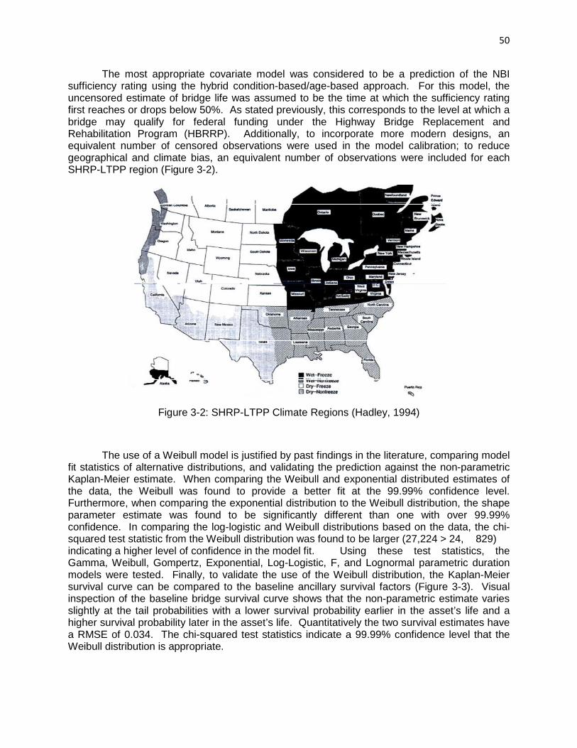
50
The most appropriate covariate model was considered to be a prediction of the NBI sufficiency rating using the hybrid condition-based/age-based approach. For this model, the uncensored estimate of bridge life was assumed to be the time at which the sufficiency rating first reaches or drops below 50%. As stated previously, this corresponds to the level at which a bridge may qualify for federal funding under the Highway Bridge Replacement and Rehabilitation Program (HBRRP). Additionally, to incorporate more modern designs, an equivalent number of censored observations were used in the model calibration; to reduce geographical and climate bias, an equivalent number of observations were included for each SHRP-LTPP region (Figure 3-2).
Figure 3-2: SHRP-LTPP Climate Regions (Hadley, 1994)
The use of a Weibull model is justified by past findings in the literature, comparing model fit statistics of alternative distributions, and validating the prediction against the non-parametric Kaplan-Meier estimate. When comparing the Weibull and exponential distributed estimates of the data, the Weibull was found to provide a better fit at the 99.99% confidence level. Furthermore, when comparing the exponential distribution to the Weibull distribution, the shape parameter estimate was found to be significantly different than one with over 99.99% confidence. In comparing the log-logistic and Weibull distributions based on the data, the chi-squared test statistic from the Weibull distribution was found to be larger (27,224 > 24, 829) indicating a higher level of confidence in the model fit. Using these test statistics, the Gamma, Weibull, Gompertz, Exponential, Log-Logistic, F, and Lognormal parametric duration models were tested. Finally, to validate the use of the Weibull distribution, the Kaplan-Meier survival curve can be compared to the baseline ancillary survival factors (Figure 3-3). Visual inspection of the baseline bridge survival curve shows that the non-parametric estimate varies slightly at the tail probabilities with a lower survival probability earlier in the asset’s life and a higher survival probability later in the asset’s life. Quantitatively the two survival estimates have a RMSE of 0.034. The chi-squared test statistics indicate a 99.99% confidence level that the Weibull distribution is appropriate.

51
Figure 3-3: Non-parametric Validation of Weibull-distributed Bridge Life Covariate Model
Given the strong fit of the Weibull distribution in describing the likelihood of bridge life, the baseline parameters and covariate influence found using maximum likelihood estimation are considered representative. The model (Table 3-7) estimates a baseline median life of 60 years with a 90% confidence interval of [22, 105]. All life expectancy factors included in the model were found to be significant at or above the 90% confidence level.
Of the significant covariates, only the indicator fur rural bridges was found to have a positive influence on bridge life. The life expectancy factors found to have a negative influence on bridge life included: warmer temperatures, increased precipitation, on the NHS, in a corrosive soil environment, steel structures, and longer structure lengths. The influences of each are considered mostly intuitive, considering:
• Warmer temperatures may lead to additional expansion forces and weaker soil strength, hence lowering asset life;
• Increased precipitation likely increases corrosion rates and disperses de-icing chemicals and other roadway by-products to the structure;
• Rural structures experience less traffic loading and congestion (factor in replacement due to insufficient bridge width) resulting in longer life;
• NHS structures accommodate more traffic loadings and higher percentages of trucks leading to potential structural problems as well as congestion which may require roadway widening. However, the data statistics suggested that NHS structures may be longer lived, possibly due to more stringent designs;
• Corrosive soils likely cause shorter substructure life; • Steel structures may be more susceptible to climate than concrete if not properly
maintained (e.g., painted); • Longer structures indicating more potential for cracking at span connections,
substructure exposure to water for over-water bridges, increased moments of forces depending on the number of spans, and potential for higher traffic volumes;
0.0
0.1
0.2
0.3
0.4
0.5
0.6
0.7
0.8
0.9
1.0
0 20 40 60 80 100
Su
rviv
al
Pro
ba
bil
ity
Age (years)
K-M
Weibull

52
Table 3-7: Weibull Regression Model of Bridge Service Life (End-of-life ≡ Age when Sufficiency Rating drops to or below 50%)
Life Expectancy Factor Parameter Estimate, β t-Statistic
Constant 4.669 218.699 Normal Annual Temperature (°F) -0.628E-2 -17.199 Normal Annual Precipitation (in.) -0.167E-2 -8.674 Geographical classification indicator (1 if rural, 0 otherwise)
0.459E-1 6.474
NHS indicator (1 if on NHS, 0 otherwise) -0.697E-1 -8.138 Corrosive soil indicator (1 if in area where average soil is classified as highly corrosive to steel or concrete by the NRCS, 0 otherwise)
-0.614E-1 -11.126
Material type indicator (1 if steel, 0 otherwise) -0.357E-1 -6.549 Structure length in decimeters -0.765E-5 -6.035
Baseline Ancillary Factors Parameter Estimate, β
t-Statistic
Shape Factor, β 2.623 185.168 Scaling Factor, α 68.871 363.000
Model Statistics Number of Observations 42,902 Log-likelihood Function at Convergence -26,785.79 Restricted Log-likelihood Function -40,397.73
Further analysis of this model is presented in Chapter 5, specifically in consideration of the sensitivity and risk of uncertain inputs.
In addition to the covariate-based model, non-covariate models were calibrated using the Markov/Weibull and Markov/Beta modeling techniques for multiple replacement rationale or ‘failure mechanisms’. This approach is considered more preferable when an agency lacks historical information but does maintain inspection records, wishes to update service life predictions based on an asset’s current age and condition rating, and seeks to identify life extension activities that can be tailored to prolonging the dominant failure mechanism.
Similar to the validation of the baseline survival curve to the Kaplan Meier, this approach compares parametric survival curves to the Markov Chain estimate. Having validated the use of the Weibull distribution, Markov/Weibull models were used to predict the overall service life of newly constructed assets. To predict the remaining service life, however, the Beta distribution was found to be more flexible and representative. Li & Sinha (2004) similarly found the Beta distribution to best represent remaining service life, particularly after a treatment.
Given a time-series of inspections, the frequency approach was used to estimate the transition probabilities for each failure mechanism. All pairs of annual and biannual NBI inspections from 1992 to 2009 were analyzed for the estimation of Markov transition probabilities on a state-by-state basis as well as for all 50 states combined. With the assumption of a one-step deterioration (i.e., only negative, unit changes in condition-state per unit time – valid assumption for ~98% of data observations), discrete-time Markov chain, the annual transition probabilities were calculated for each age range (transition matrices calibrated for each 6 years of life) by:

53
l�� � M�� � �N�� 2 °�[� � °�
Where: aii represents the number of annual inspection pairs staying in state i from one year to the next; bii represents the number of biannual inspection pairs where no condition state change was observed; Ai represents the number of annual inspection pairs starting in state I; Bi represents the number of biannual inspection pairs starting in state i.
This simplified equation represents the weighted transition probabilities based on the number of annual and biannual inspections. The paired transition probability is then l�� � 1 � l��. Using the transition matrix, the Markov/Weibull and Markov/Beta models was then calibrated by minimizing the RMSE while holding the median life prediction constant and changing the baseline ancillary survival factors. When no observations were available, a 100% transition probability was assumed. Models were fit to the following set of discrete ratings included in the NBI (full descriptions in Appendix A):
• Deck Condition Rating – represents condition state of deck on a 0-9 scale; • Superstructure Condition Rating – represents condition state of superstructure on a 0-9
scale ; • Substructure Condition Rating – represents condition state of substructure on a 0-9
scale; • Deck Geometry Rating – represents functional acceptability based on roadway width,
traffic volume, and vertical clearance on a 0-9 scale. The Markov transitions for this rating pertain to the change in traffic volume levels;
• Channel Protection Rating – represents condition state of channel/embankment on a 0-9 scale;
• Scour Protection Rating – represents condition state of structures susceptible to scour on a 0-5 scale (ratings above 5 indicate a bridge is either not susceptible, already repaired, or not investigated)
The results of the analysis are limited to the data quality and number of available observations and can be updated based on the preferred transition probabilities. For instance, far fewer observations are available for assessing deterioration due to scour than other ratings, therefore the Weibull parameters and life predictions for this failure mechanism are considered less reflective of actual conditions than the models calibrated based on the other ratings.
Using the previously described approach, the transition matrices from Table 3-8 through Table 3-13 were used to calibrate the Weibull parameters and predict the median life estimates. In order to update future transition probabilities, the number of observations for each model are also provided in Table 3-14 through Table 3-19. Markov/Weibull transition matrices, number of observations, and Weibull predictions and factors for each U.S. state were obtained (e.g., see Indiana data analyzed later in this study in Appendix B). The average life based on all observations for each failure mechanism and sorted by threshold are summarized in Table 3-20.

54
Table 3-8: Bridge Deck Transition Matrices for All Observations
Age Group Annual Transition Probabilities
9 → 8 8 → 7 7 → 6 6 → 5 5 → 4 4 → 3 0 → 6 years 23.04 11.02 4.65 5.03 3.31 4.69 7 → 12 yrs 17.44 10.19 4.94 5.53 4.90 6.22 13 → 18 yrs 16.43 9.98 5.33 5.61 5.36 4.84 19 → 24 yrs 22.26 11.79 6.18 6.18 5.46 4.79 25 → 30 yrs 32.23 13.50 6.97 6.33 5.62 4.49 31 → 36 yrs 36.35 15.33 7.49 6.25 5.95 4.50 37 → 42 yrs 38.95 15.80 7.74 6.24 5.84 4.24 43 → 48 yrs 36.84 17.66 8.14 6.66 5.50 4.76 49 → 54 yrs 33.08 18.00 8.92 7.09 5.29 4.57 55 → 60 yrs 30.69 17.88 10.64 7.90 5.40 4.66 61 → 66 yrs 36.51 18.93 10.41 7.75 5.44 4.31 67 → 72 yrs 39.12 18.36 10.84 7.71 5.42 4.36 73 → 78 yrs 46.86 20.40 11.37 8.20 5.51 4.54 79 → 84 yrs 27.02 21.85 13.49 9.72 6.51 4.86 85 → 90 yrs 38.78 25.40 15.75 12.42 7.74 5.17 91 → 96 yrs 36.97 22.84 16.23 12.64 7.88 6.12 97 → 102 yrs 33.20 19.73 13.42 11.24 8.67 6.90 103 → 108 yrs 17.49 16.36 12.45 10.39 6.67 5.73 109 → 114 yrs 33.33 29.50 11.97 14.70 9.16 12.61 115 → 120 yrs 59.76 24.33 18.29 10.19 8.57 5.52
Table 3-9: Bridge Superstructure Transition Matrices for All Observations
Age Group Annual Transition Probabilities
9 → 8 8 → 7 7 → 6 6 → 5 5 → 4 4 → 3 0 → 6 years 20.08 6.43 4.73 4.58 4.03 4.86 7 → 12 yrs 15.55 6.85 4.57 5.19 4.95 6.10 13 → 18 yrs 15.36 7.29 4.80 5.56 5.53 6.01 19 → 24 yrs 19.59 8.74 5.25 5.82 5.48 5.93 25 → 30 yrs 29.61 10.54 5.65 5.80 5.47 5.96 31 → 36 yrs 30.73 12.34 6.07 5.77 5.35 5.34 37 → 42 yrs 32.96 13.81 6.39 5.79 5.42 4.98 43 → 48 yrs 31.82 15.67 7.23 6.10 5.44 5.51 49 → 54 yrs 27.81 16.27 8.14 6.72 5.64 5.18 55 → 60 yrs 34.31 16.60 9.55 7.15 5.85 4.77 61 → 66 yrs 34.61 16.56 9.30 7.35 5.72 4.60 67 → 72 yrs 33.87 15.65 9.84 7.43 5.85 4.63 73 → 78 yrs 37.74 16.92 9.83 7.55 6.02 4.96 79 → 84 yrs 21.51 17.26 10.98 8.89 6.52 5.68 85 → 90 yrs 37.04 18.81 12.88 10.65 7.28 6.54 91 → 96 yrs 33.39 18.93 14.98 11.39 9.02 7.03 97 → 102 yrs 30.14 19.25 12.53 10.56 8.22 7.10 103 → 108 yrs 15.94 14.80 11.35 8.78 7.52 6.31 109 → 114 yrs 20.00 31.82 12.18 13.25 8.58 4.83 115 → 120 yrs 0.00 8.33 16.45 10.77 10.93 7.82
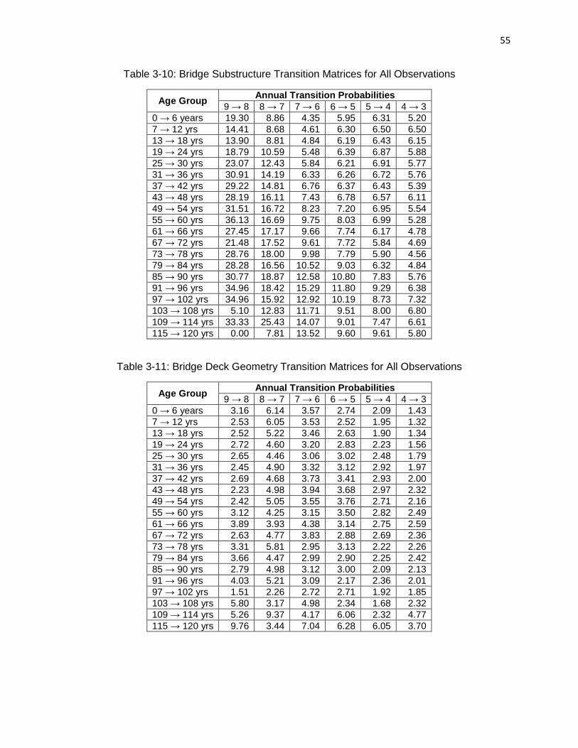
55
Table 3-10: Bridge Substructure Transition Matrices for All Observations
Age Group Annual Transition Probabilities
9 → 8 8 → 7 7 → 6 6 → 5 5 → 4 4 → 3 0 → 6 years 19.30 8.86 4.35 5.95 6.31 5.20 7 → 12 yrs 14.41 8.68 4.61 6.30 6.50 6.50 13 → 18 yrs 13.90 8.81 4.84 6.19 6.43 6.15 19 → 24 yrs 18.79 10.59 5.48 6.39 6.87 5.88 25 → 30 yrs 23.07 12.43 5.84 6.21 6.91 5.77 31 → 36 yrs 30.91 14.19 6.33 6.26 6.72 5.76 37 → 42 yrs 29.22 14.81 6.76 6.37 6.43 5.39 43 → 48 yrs 28.19 16.11 7.43 6.78 6.57 6.11 49 → 54 yrs 31.51 16.72 8.23 7.20 6.95 5.54 55 → 60 yrs 36.13 16.69 9.75 8.03 6.99 5.28 61 → 66 yrs 27.45 17.17 9.66 7.74 6.17 4.78 67 → 72 yrs 21.48 17.52 9.61 7.72 5.84 4.69 73 → 78 yrs 28.76 18.00 9.98 7.79 5.90 4.56 79 → 84 yrs 28.28 16.56 10.52 9.03 6.32 4.84 85 → 90 yrs 30.77 18.87 12.58 10.80 7.83 5.76 91 → 96 yrs 34.96 18.42 15.29 11.80 9.29 6.38 97 → 102 yrs 34.96 15.92 12.92 10.19 8.73 7.32 103 → 108 yrs 5.10 12.83 11.71 9.51 8.00 6.80 109 → 114 yrs 33.33 25.43 14.07 9.01 7.47 6.61 115 → 120 yrs 0.00 7.81 13.52 9.60 9.61 5.80
Table 3-11: Bridge Deck Geometry Transition Matrices for All Observations
Age Group Annual Transition Probabilities
9 → 8 8 → 7 7 → 6 6 → 5 5 → 4 4 → 3 0 → 6 years 3.16 6.14 3.57 2.74 2.09 1.43 7 → 12 yrs 2.53 6.05 3.53 2.52 1.95 1.32 13 → 18 yrs 2.52 5.22 3.46 2.63 1.90 1.34 19 → 24 yrs 2.72 4.60 3.20 2.83 2.23 1.56 25 → 30 yrs 2.65 4.46 3.06 3.02 2.48 1.79 31 → 36 yrs 2.45 4.90 3.32 3.12 2.92 1.97 37 → 42 yrs 2.69 4.68 3.73 3.41 2.93 2.00 43 → 48 yrs 2.23 4.98 3.94 3.68 2.97 2.32 49 → 54 yrs 2.42 5.05 3.55 3.76 2.71 2.16 55 → 60 yrs 3.12 4.25 3.15 3.50 2.82 2.49 61 → 66 yrs 3.89 3.93 4.38 3.14 2.75 2.59 67 → 72 yrs 2.63 4.77 3.83 2.88 2.69 2.36 73 → 78 yrs 3.31 5.81 2.95 3.13 2.22 2.26 79 → 84 yrs 3.66 4.47 2.99 2.90 2.25 2.42 85 → 90 yrs 2.79 4.98 3.12 3.00 2.09 2.13 91 → 96 yrs 4.03 5.21 3.09 2.17 2.36 2.01 97 → 102 yrs 1.51 2.26 2.72 2.71 1.92 1.85 103 → 108 yrs 5.80 3.17 4.98 2.34 1.68 2.32 109 → 114 yrs 5.26 9.37 4.17 6.06 2.32 4.77 115 → 120 yrs 9.76 3.44 7.04 6.28 6.05 3.70

56
Table 3-12: Bridge Channel Protection Transition Matrices for All Observations
Age Group Annual Transition Probabilities
9 → 8 8 → 7 7 → 6 6 → 5 5 → 4 4 → 3 0 → 6 years 18.76 8.04 6.29 4.23 2.96 2.42 7 → 12 yrs 10.87 7.83 6.13 4.33 3.23 1.91 13 → 18 yrs 10.88 7.58 5.94 4.14 3.31 1.99 19 → 24 yrs 11.41 7.81 6.15 4.03 3.25 1.95 25 → 30 yrs 8.96 8.10 6.04 3.99 3.26 1.90 31 → 36 yrs 8.72 8.51 6.19 4.11 3.03 2.20 37 → 42 yrs 9.59 8.66 6.16 4.08 3.12 1.95 43 → 48 yrs 8.73 8.63 6.35 4.14 2.99 1.71 49 → 54 yrs 9.89 9.62 7.06 4.37 3.26 1.63 55 → 60 yrs 10.62 9.82 7.43 4.72 3.19 1.43 61 → 66 yrs 12.17 10.30 7.67 4.88 3.30 1.55 67 → 72 yrs 12.45 9.60 7.44 4.96 3.27 1.27 73 → 78 yrs 8.68 9.20 7.79 5.20 3.31 1.62 79 → 84 yrs 8.31 9.79 8.09 5.34 3.48 1.71 85 → 90 yrs 14.10 10.79 9.32 5.81 3.45 2.13 91 → 96 yrs 16.59 15.82 12.96 6.60 3.87 3.28 97 → 102 yrs 26.10 13.11 10.53 6.73 3.99 3.16 103 → 108 yrs 18.47 10.79 10.12 4.74 3.62 2.94 109 → 114 yrs 12.50 9.52 8.43 6.66 2.34 2.16 115 → 120 yrs 100.00 12.29 8.90 4.82 6.98 1.74
Table 3-13: Bridge Scour Protection Transition Matrices for All Observations
Age Group Annual Transition Probabilities
5 → 4 4 → 3 3 → 2 0 → 6 years 0.01 0.19 0.04 7 → 12 yrs 0.02 0.07 0.01 13 → 18 yrs 0.01 0.14 0.03 19 → 24 yrs 0.01 0.23 0.01 25 → 30 yrs 0.01 0.16 0.01 31 → 36 yrs 0.01 0.09 0.01 37 → 42 yrs 0.02 0.07 0.01 43 → 48 yrs 0.02 0.10 0.01 49 → 54 yrs 0.03 0.14 0.01 55 → 60 yrs 0.05 0.16 0.04 61 → 66 yrs 0.04 0.16 0.02 67 → 72 yrs 0.05 0.17 0.01 73 → 78 yrs 0.09 0.06 0.02 79 → 84 yrs 0.06 0.28 0.13 85 → 90 yrs 0.18 0.36 0.04 91 → 96 yrs 0.09 0.15 0.09 97 → 102 yrs 0.05 0.14 0.11 103 → 108 yrs 0.28 1.43 0.11 109 → 114 yrs 0.61 3.31 0.06 115 → 120 yrs 0.33 0.45 0.60
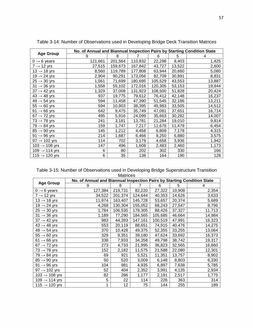
57
Table 3-14: Number of Observations used in Developing Bridge Deck Transition Matrices
Age Group No. of Annual and Biannual Inspection Pairs by Star ting Condition State
9 8 7 6 5 4 0 → 6 years 121,661 201,564 110,832 22,298 8,403 1,425 7 → 12 yrs 27,515 159,673 167,842 43,727 13,522 2,600 13 → 18 yrs 8,560 119,789 177,808 63,944 20,660 5,080 19 → 24 yrs 2,904 90,291 173,056 82,709 30,891 8,831 25 → 30 yrs 1,561 71,699 180,695 105,529 43,553 13,887 31 → 36 yrs 1,558 55,102 172,016 120,305 53,153 19,944 37 → 42 yrs 1,329 37,008 131,923 108,500 51,828 20,424 43 → 48 yrs 937 19,775 79,612 76,412 42,148 16,237 49 → 54 yrs 594 11,458 47,390 51,545 32,186 13,211 55 → 60 yrs 594 10,903 38,395 45,983 33,505 14,512 61 → 66 yrs 642 9,475 35,749 47,081 37,651 16,714 67 → 72 yrs 495 5,916 24,099 35,663 30,282 14,007 73 → 78 yrs 241 3,181 13,781 21,284 19,010 9,814 79 → 84 yrs 159 1,747 7,217 11,676 11,479 6,454 85 → 90 yrs 145 1,212 4,458 6,808 7,178 4,315 91 → 96 yrs 214 1,687 6,466 8,250 6,880 3,575 97 → 102 yrs 114 702 3,179 4,658 3,936 1,942 103 → 108 yrs 147 496 1,608 2,483 2,460 1,173 109 → 114 yrs 6 80 202 302 330 166 115 → 120 yrs 6 35 138 164 190 128
Table 3-15: Number of Observations used in Developing Bridge Superstructure Transition Matrices
Age Group No. of Annual and Biannual Inspection Pairs by Star ting Condition State
9 8 7 6 5 4 0 → 6 years 127,384 219,731 82,220 27,322 10,908 2,354 7 → 12 yrs 34,522 201,374 124,644 40,353 14,626 3,633 13 → 18 yrs 11,974 163,407 145,728 53,657 20,374 5,689 19 → 24 yrs 4,268 130,304 155,052 68,243 27,547 8,796 25 → 30 yrs 1,784 106,535 178,305 88,426 37,327 11,713 31 → 36 yrs 1,189 77,290 184,565 105,685 46,664 14,984 37 → 42 yrs 983 44,393 147,161 100,519 47,991 16,323 43 → 48 yrs 553 20,119 88,651 74,915 40,476 14,275 49 → 54 yrs 370 10,428 49,375 52,355 33,255 13,064 55 → 60 yrs 329 9,351 39,180 47,624 33,692 16,373 61 → 66 yrs 338 7,933 34,358 49,798 38,742 19,317 67 → 72 yrs 273 4,733 21,995 36,823 32,565 16,860 73 → 78 yrs 152 2,182 11,575 21,588 22,080 12,301 79 → 84 yrs 69 921 5,521 11,351 13,757 8,902 85 → 90 yrs 50 520 3,009 6,148 8,803 6,330 91 → 96 yrs 104 981 4,935 6,897 7,638 5,785 97 → 102 yrs 52 404 2,352 3,991 4,135 2,934 103 → 108 yrs 82 286 1,177 2,191 2,517 1,775 109 → 114 yrs 5 22 114 226 363 314 115 → 120 yrs 1 12 75 144 255 189
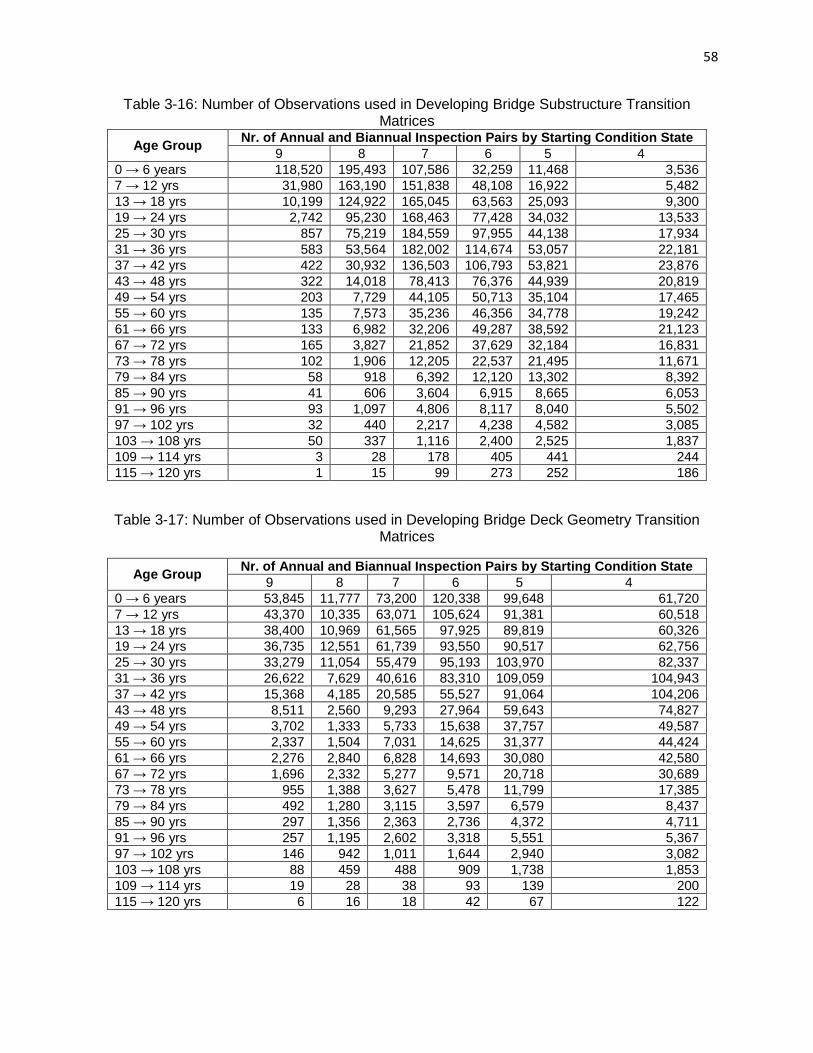
58
Table 3-16: Number of Observations used in Developing Bridge Substructure Transition Matrices
Age Group Nr. of Annual and Biannual Inspection Pairs by Starting Condition State
9 8 7 6 5 4 0 → 6 years 118,520 195,493 107,586 32,259 11,468 3,536 7 → 12 yrs 31,980 163,190 151,838 48,108 16,922 5,482 13 → 18 yrs 10,199 124,922 165,045 63,563 25,093 9,300 19 → 24 yrs 2,742 95,230 168,463 77,428 34,032 13,533 25 → 30 yrs 857 75,219 184,559 97,955 44,138 17,934 31 → 36 yrs 583 53,564 182,002 114,674 53,057 22,181 37 → 42 yrs 422 30,932 136,503 106,793 53,821 23,876 43 → 48 yrs 322 14,018 78,413 76,376 44,939 20,819 49 → 54 yrs 203 7,729 44,105 50,713 35,104 17,465 55 → 60 yrs 135 7,573 35,236 46,356 34,778 19,242 61 → 66 yrs 133 6,982 32,206 49,287 38,592 21,123 67 → 72 yrs 165 3,827 21,852 37,629 32,184 16,831 73 → 78 yrs 102 1,906 12,205 22,537 21,495 11,671 79 → 84 yrs 58 918 6,392 12,120 13,302 8,392 85 → 90 yrs 41 606 3,604 6,915 8,665 6,053 91 → 96 yrs 93 1,097 4,806 8,117 8,040 5,502 97 → 102 yrs 32 440 2,217 4,238 4,582 3,085 103 → 108 yrs 50 337 1,116 2,400 2,525 1,837 109 → 114 yrs 3 28 178 405 441 244 115 → 120 yrs 1 15 99 273 252 186
Table 3-17: Number of Observations used in Developing Bridge Deck Geometry Transition Matrices
Age Group Nr. of Annual and Biannual Inspection Pairs by Starti ng Condition State
9 8 7 6 5 4 0 → 6 years 53,845 11,777 73,200 120,338 99,648 61,720 7 → 12 yrs 43,370 10,335 63,071 105,624 91,381 60,518 13 → 18 yrs 38,400 10,969 61,565 97,925 89,819 60,326 19 → 24 yrs 36,735 12,551 61,739 93,550 90,517 62,756 25 → 30 yrs 33,279 11,054 55,479 95,193 103,970 82,337 31 → 36 yrs 26,622 7,629 40,616 83,310 109,059 104,943 37 → 42 yrs 15,368 4,185 20,585 55,527 91,064 104,206 43 → 48 yrs 8,511 2,560 9,293 27,964 59,643 74,827 49 → 54 yrs 3,702 1,333 5,733 15,638 37,757 49,587 55 → 60 yrs 2,337 1,504 7,031 14,625 31,377 44,424 61 → 66 yrs 2,276 2,840 6,828 14,693 30,080 42,580 67 → 72 yrs 1,696 2,332 5,277 9,571 20,718 30,689 73 → 78 yrs 955 1,388 3,627 5,478 11,799 17,385 79 → 84 yrs 492 1,280 3,115 3,597 6,579 8,437 85 → 90 yrs 297 1,356 2,363 2,736 4,372 4,711 91 → 96 yrs 257 1,195 2,602 3,318 5,551 5,367 97 → 102 yrs 146 942 1,011 1,644 2,940 3,082 103 → 108 yrs 88 459 488 909 1,738 1,853 109 → 114 yrs 19 28 38 93 139 200 115 → 120 yrs 6 16 18 42 67 122

59
Table 3-18: Number of Observations used in Developing Bridge Channel Protection Transition Matrices
Age Group No. of Annual and Biannual Inspection Pairs by Star ting Condition State
9 8 7 6 5 4 0 → 6 years 51,391 158,989 97,624 41,327 10,725 2,305 7 → 12 yrs 15,693 120,078 109,857 55,537 15,719 3,730 13 → 18 yrs 7,366 97,674 109,966 65,519 20,596 5,272 19 → 24 yrs 4,122 83,035 104,530 69,587 24,046 6,681 25 → 30 yrs 3,484 79,840 107,015 75,216 26,764 7,407 31 → 36 yrs 3,580 75,240 109,946 80,298 30,006 8,257 37 → 42 yrs 2,854 60,928 97,378 75,868 29,507 8,243 43 → 48 yrs 1,882 38,335 69,749 60,928 25,277 7,006 49 → 54 yrs 1,080 25,631 48,046 45,833 20,428 6,102 55 → 60 yrs 841 23,844 42,954 44,270 22,425 7,788 61 → 66 yrs 739 23,453 42,494 47,636 24,376 8,424 67 → 72 yrs 597 16,214 30,682 36,903 20,353 6,888 73 → 78 yrs 352 9,301 18,485 23,592 13,699 4,728 79 → 84 yrs 217 5,537 10,558 13,816 8,895 3,219 85 → 90 yrs 128 3,386 6,553 8,601 5,980 2,220 91 → 96 yrs 169 3,441 8,577 9,388 5,127 1,778 97 → 102 yrs 98 1,418 3,988 5,456 3,276 912 103 → 108 yrs 84 897 2,032 3,145 1,921 631 109 → 114 yrs 8 225 417 445 218 97 115 → 120 yrs 1 121 266 304 139 60
Table 3-19: Number of Observations used in Developing Bridge Scour Protection Transition Matrices
Age Group No. of Annual and Biannual Inspection Pairs by Starting Condition State
5 4 3 0 → 6 years 31,935 5,263 2,931 7 → 12 yrs 32,094 5,594 4,250 13 → 18 yrs 33,380 5,894 6,184 19 → 24 yrs 33,642 5,516 7,289 25 → 30 yrs 34,946 5,744 8,461 31 → 36 yrs 36,688 6,185 9,142 37 → 42 yrs 32,855 5,930 10,801 43 → 48 yrs 24,053 5,253 10,014 49 → 54 yrs 15,083 4,058 6,584 55 → 60 yrs 10,663 4,188 4,296 61 → 66 yrs 12,236 5,271 5,583 67 → 72 yrs 11,821 4,514 6,001 73 → 78 yrs 8,882 2,791 3,973 79 → 84 yrs 5,332 1,470 2,024 85 → 90 yrs 3,864 915 1,231 91 → 96 yrs 3,669 896 836 97 → 102 yrs 3,458 543 564 103 → 108 yrs 2,095 327 263 109 → 114 yrs 149 43 81 115 → 120 yrs 77 34 63

60
Table 3-20: Markov/Weibull Model Predictions of Bridge Service Life by Failure Mechanism for All Observations
Failure Mechanism
End-of-Life Threshold
Average Life
(years)
90% Confidence
Interval
Weibull Scaling
Factor, α
Weibull Shape
Factor, β
Deck Condition Rating
5 42 [15,75] 48.62 2.50 4 58 [22,100] 66.44 2.70 3 79 [36,123] 88.33 3.28
Superstructure Condition Rating
5 48 [18,83] 55.03 2.68 4 64 [27,104] 72.26 3.02 3 83 [40,125] 91.97 3.57
Substructure Condition Rating
5 45 [16,79] 51.84 2.59 4 59 [23,100] 67.36 2.77 3 78 [34,124] 87.62 3.15
Deck Geometry Rating
5 >120* N/A N/A N/A 4 >120* N/A N/A N/A 3 110 [35,209] 129.24 2.27
Channel Protection Rating
5 53 [17,100] 62.20 2.29 4 81 [31,139] 92.77 2.70 3 120 [56,183] 133.43 3.45
Scour Protection Rating
4 >120* N/A N/A N/A 3 >120* N/A N/A N/A 2 >120* N/A N/A N/A
*Insufficient observations for predictions of Asset Life beyond 120 years
It was found that on average that decks tend to have a service life varying from 42 to 79 years, threshold dependent. Given the general lack of inspection pairs beginning at a state equal to or below 5 (only 9.27% of paired observations), a threshold of 5 is considered appropriate. The 42 year life corresponding to this threshold compares well with the life expectancy values in the literature (~25 to 50 year average deck life expectancy). A root mean square error (RMSE) of 0.99 was calculated in comparing the Markov prediction to the Weibull model for the identified threshold.
For superstructures, average service life estimates varied from 48 to 83 years, depending on the threshold. Again with 6.70% of the paired observations having a starting condition rating of below 4, this threshold is considered appropriate. This prediction of 64 years compares favorably to the literature (~50 to 80 year average superstructure life expectancy). A RMSE value of 0.76 was found.
Substructures on average were found to survive between 45 and 78 years depending on the threshold. The 59 year prediction corresponding to threshold 4 was found to be within the range of estimates in the literature (~25 to 80 year average substructure life expectancy). A RMSE of 1.21 was calculated for the corresponding threshold.
Service life based on the deck geometry rating were significantly higher than the life predictions for the bridge elements. With average life values over 110 years, this replacement rationale is not considered likely to dominate. Only 10% of inspection pairs had an initial value below a condition state of 3, therefore a threshold of 3 was assumed.

61
Observed transition probabilities for the channel ratings suggest an average life varying from 53 to 120 years. With only 3.69% of inspection pairs beginning at a condition state of 4 or lower, a threshold of 4 is considered appropriate. This threshold corresponds to a life prediction of 81 years on average, with a RMSE of 0.85.
Similar to deck geometry ratings, the life prediction based on scour were found to be well above that of the element condition ratings. With the limited number of observations, relative to the other ratings, average life was estimated at over 120 years. A threshold of 2 is assumed given that only 9.47 percent of inspection pairs start in an equal or worse condition state.
Combining all the possible replacement rationale and identified thresholds, it can be seen that decks on average survive 42 years, while the entire bridge structure has a life of 59 years based on the dominating substructure rating. This estimate is nearly identical to that of the covariate model, which predicted an overall, average bridge life of 60 years.
A comparison of predictions by SHRP-LTPP region was similarly completed using the identified thresholds (Table 3-21). Insufficient observations were available for estimating life based on scour at this geographic level. Overall, it was found that bridges in the Northeast region had a median life of 56 years; Northwestern bridges had a median life of 70 years; bridges in the Southeast had an average life of 58 years; and the median life of bridges in the Southwest was found to be 65 years. This finding suggests that eastern bridges, coinciding with wetter climates, have a shorter overall life by approximately 7 to 14 years than their northern and southern counterparts. Minor differences in life were found between northern and southern geographic splits, indicating that freezing climatic conditions may not significantly affect bridge life.
The dominating failure mechanism for each SHRP-LTPP region was the substructure rating. This would suggest that life extension activities for the substructure would likely be needed for longer-lived superstructures (e.g., stainless steel reinforcement). The bridges in the Northeast region had the lowest substructure life, which was consistent with all other failure mechanisms except deck geometry. The longest-lived substructures and superstructures, on average, were found in the Northwest; the longest-lived decks and channels were found in the Southeast.
One of the benefits of the Markov technique is the ability to adjust life predictions based on the current asset age and condition state. If the assumption of new construction in condition state 9 (or 5 for scour protection) is relaxed, then the median life predictions for the identified thresholds and for each failure mechanism using all observations are obtained (Figure 3-4 through Figure 3-9). The uptick at later ages from the Markovian prediction are the result of a lack of observations in the later age groups. Individual Beta distributions can be created for each combination of condition states and age.
Using the developed figures, it can be seen for instance that a 60 year old asset with deck rating = 6, superstructure rating = 6, substructure rating = 5, deck geometry rating = 6, channel protection rating = 6, and not susceptible to scour, would be estimated to have the following median remaining service life (RSL) deck - 9 years, superstructure - 25 years, substructure - 12 years, deck geometry - 82 years, and channel protection - 39 years. As such the agency can see that some activity to extend the deck life 3 years may be needed in order to replace the entire bridge in 12 years based on an inadequate substructure. Similar applications will be discussed in the following chapter in more detail.

62
Table 3-21: Markov/Weibull Model Predictions of Bridge Service Life by Failure Mechanism and SHRP-LTPP Region
Failure Mechanism and
Threshold
SHRP-LTPP Region
Average Life
(years)
90% Confidence
Interval
Weibull Scaling
Factor, α
Weibull Shape
Factor, β
Deck Condition Rating = 5
NE 37 [13,66] 42.73 2.54 NW 49 [19,84] 56.02 2.74 SE 50 [20,85] 57.04 2.78 SW 39 [10,83] 47.06 1.95
Superstructure Condition Rating = 4
NE 57 [23,95] 64.76 2.87 NW 80 [42,115] 87.66 4.01 SE 69 [33,105] 76.71 3.46 SW 78 [37,120] 86.80 3.43
Substructure Condition Rating = 4
NE 56 [22,95] 63.90 2.78 NW 70 [31,110] 78.42 3.23 SE 58 [23,97] 65.90 2.87 SW 65 [21,123] 76.32 2.28
Deck Geometry Condition Rating = 3
NE >120 N/A N/A N/A NW >120 N/A N/A N/A SE 112 [97,122] 114.33 17.80 SW >120 N/A N/A N/A
Channel Protection Condition Rating = 4
NE 65 [23,118] 75.46 2.46 NW 108 [54,159] 118/93 3.80 SE 109 [47,175] 122.66 3.10 SW 94 [33,169] 108.82 2.50
Scour Protection Condition Rating = 2
NE >120 N/A N/A N/A NW >120 N/A N/A N/A SE >100 N/A N/A N/A SW >100 N/A N/A N/A
Figure 3-4: Bridge Deck Median RSL by Age and Current Rating
0
5
10
15
20
25
30
35
40
45
0 20 40 60 80 100 120
RS
L in
Ye
ars
Age in Years
Current State = 9
Current State = 8
Current State = 7
Current State = 6

63
Figure 3-5: Bridge Superstructure Median RSL by Age and Current Rating
Figure 3-6: Bridge Substructure Median RSL by Age and Current Rating
0
10
20
30
40
50
60
70
0 20 40 60 80 100 120
RS
L in
Ye
ars
Age in Years
Current State = 9
Current State = 8
Current State = 7
Current State = 6
Current State = 5
0
10
20
30
40
50
60
70
0 20 40 60 80 100 120
RS
L in
Ye
ars
Age in Years
Current State = 9
Current State = 8
Current State = 7
Current State = 6
Current State = 5

64
Figure 3-7: Bridge Deck Geometry Median RSL by Age and Current Rating
Figure 3-8: Bridge Channel Protection Median RSL by Age and Current Rating
0
20
40
60
80
100
120
140
160
0 20 40 60 80 100 120
RS
L in
Ye
ars
Age in Years
Current State = 9
Current State = 8
Current State = 7
Current State = 6
Current State = 5
Current State = 4
0
10
20
30
40
50
60
70
80
90
0 20 40 60 80 100 120
RS
L in
Ye
ars
Age in Years
Current State = 9
Current State = 8
Current State = 7
Current State = 6
Current State = 5

65
Figure 3-9: Bridge Scour Protection Median RSL by Age and Current Rating
3.3.2 Box Culverts
Given the variety of structures labeled as ‘culverts’, the data was analyzed within two distinctive classifications: (1) large (> 20 feet road length), typically concrete box culverts in the NBI database, and (2) small, typically plastic or metal pipe culverts, found in DOT in-house databases. As with the analysis of bridges, both covariate and non-covariate models were calibrated for the prediction of box culvert life using the NBI database. The covariate model was used to identify significant life expectancy factors and to predict the structural service life of box culverts. The non-covariate technique was applied to predict the life due to multiple rationale or ‘failure mechanisms’.
For box culverts, insufficient data is available for the calculation of the NBI sufficiency rating (i.e., deck geometry), therefore the culvert condition rating was estimated using the hybrid condition-based/age-based method. For this model, the uncensored estimates of culvert life were assumed to be (i) historical replacement record (‘year of reconstruction’ NBI data field – ‘year built’ NBI data field) and (ii) the time at which the culvert condition rating first reaches or drops below condition state 3. An equivalent number of censored observations were used in the model calibration as well as an equivalent number of observations from each SHRP-LTPP region. Similar checks as in the previous section were completed, with all results indicating that the Weibull distribution is the most appropriate model form for the data (>99.99% confidence). The fit of the model is slightly worse than that as for bridges with a RMSE of 0.096 (Figure 3-10). The covariate model (Table 3-22), calculated with maximum likelihood methods, indicates a median life of 55 years with a 90% confidence interval of [21, 94].
Factors with a significant, positive effect on life were found to include: precipitation, rural geographic setting, concrete material type, state maintenance responsibility, and structure length. Factors with a negative effect included: temperature, NHS status, Interstate classification, and soil acidity. The intuitiveness of these factors is relatively strong and consistent with the covariate bridge life model. The most surprising result was the positive influence of precipitation on culvert life, which seemingly contradicts the effect assessed for bridges. Considering that culverts are inherently hydraulic structures, the negative consequences normally associated precipitation may be mitigated by improved removal of harmful runoff. Otherwise, the finding that lower traffic volumes (i.e., rural, non-NHS, non-Interstate) have longer life estimates is not surprising, nor the negative effect of soil acidity.
0
100
200
300
400
500
0 20 40 60 80 100 120
RS
L in
Ye
ars
Age in Years
Current State = 5
Current State = 4
Current State = 3

66
While concrete structures (the predominate box culvert material type) have a higher capacity for heat retention, buckling, in part caused by the lack of soil moisture, is likely the reason that a negative effect for temperature was found (Committee on Climate Change and U.S. Transportation, National Research Council, 2008).
Figure 3-10: Non-parametric Validation of Weibull-distributed Box Culvert Life Covariate Model
Table 3-22: Weibull Regression Model of Box Culvert Service Life
Life Expectancy Factor Parameter Estimate, β t-Statistic
Constant 4.016 286.844 Normal Annual Temperature (°F) -0.323E-2 -9.760 Normal Annual Precipitation (in.) 0.322E-2 9.672
Geographical classification indicator (1 if rural, 0 otherwise) 0.843E-1
9.032
NHS indicator (1 if on NHS, 0 otherwise) -0.168E-2 -1.647 Functional class indicator (1 if on interstate, 0 otherwise) -0.250 -14.691 Maintenance responsibility indicator (1 if state responsible, 0 otherwise) 0.333E-1 4.000 Corrosive soil indicator (1 if in area where average soil is classified as highly corrosive to steel or concrete by the NRCS, 0 otherwise)
-0.853E-1 -10.944
Acidic soil indicator (1 if in area with average soil of pH < 6.5 according to NCRS, 0 otherwise)
-0.723E-1 -8.517
Material type indicator (1 if concrete, 0 otherwise) 0.270 29.887 Structure length in decimeters 0.140E-4 2.086
Baseline Ancillary Factors Parameter Estimate, β t-Statistic
Shape Factor, β 2.728 133.200 Scaling Factor, α 63.211 263.833
Model Statistics Number of Observations 19,512 Log-likelihood Function at Convergence -10,384.79 Restricted Log-likelihood Function -19,790.65 (End-of-life ≡ Historical Replacement Interval and Age when Culvert Condition Rating drops to or below 3)
As with the bridge data, Markov/Weibull and Markov/Beta models were additionally fit to the box culvert data. Due to the lack of observations for deck geometry and scour, models for the culvert condition rating and channel protection rating were analyzed. The transition matrices
0.0
0.1
0.2
0.3
0.4
0.5
0.6
0.7
0.8
0.9
1.0
0 20 40 60 80 100
Su
rviv
al
Pro
ba
bil
ity
Age (years)
K-M
Weibull

67
for the culvert condition rating and channel protection rating are provided in Table 3-23 and Table 3-24, respectively. Again, to further update the transition matrices, the number of observations is presented in Table 3-25 and Table 3-26, respectively.
Table 3-23: Box Culvert Condition Transition Matrices for All Observations
Age Group Annual Transition Probabilities
9 → 8 8 → 7 7 → 6 6 → 5 5 → 4 4 → 3 0 → 6 years 18.85 9.29 3.64 3.06 4.22 5.94 7 → 12 yrs 13.53 8.15 3.58 2.99 4.57 2.83 13 → 18 yrs 14.18 7.49 3.82 3.11 4.34 5.29 19 → 24 yrs 16.18 8.85 4.55 3.34 4.25 5.47 25 → 30 yrs 20.58 10.16 4.92 3.71 4.43 4.31 31 → 36 yrs 23.29 11.07 5.16 3.52 4.18 3.89 37 → 42 yrs 25.98 11.09 5.06 2.93 3.56 4.22 43 → 48 yrs 31.09 10.43 5.09 2.88 3.44 4.65 49 → 54 yrs 37.07 10.40 5.25 3.31 3.31 4.65 55 → 60 yrs 35.25 13.63 5.99 3.62 3.29 3.06 61 → 66 yrs 34.79 11.50 5.89 3.69 3.50 2.79 67 → 72 yrs 31.49 10.87 5.26 3.03 3.25 3.10 73 → 78 yrs 71.92 10.72 5.26 3.98 3.37 2.73 79 → 84 yrs 39.64 12.83 8.51 6.88 5.58 4.53 85 → 90 yrs 50.00 10.87 11.34 6.96 7.60 5.75 91 → 96 yrs 62.16 18.21 6.92 7.73 5.00 4.55 97 → 102 yrs 14.42 12.60 5.03 5.93 5.12 5.19 103 → 108 yrs 0.00 10.40 5.68 5.89 4.77 1.87 109 → 114 yrs 100.00 0.00 100.00 0.00 100.00 11.11 115 → 120 yrs 100.00 0.00 0.00 9.69 25.00 0.00
Table 3-24: Box Culvert Channel Protection Transition Matrices for All Observations
Age Group Annual Transition Probabilities
9 → 8 8 → 7 7 → 6 6 → 5 5 → 4 4 → 3 0 → 6 years 20.62 9.71 6.35 4.20 3.05 2.47 7 → 12 yrs 11.00 8.87 5.90 3.79 2.73 1.04 13 → 18 yrs 9.36 8.62 5.59 3.69 2.25 1.16 19 → 24 yrs 9.70 8.84 6.06 3.83 2.68 1.12 25 → 30 yrs 6.88 10.04 5.87 4.05 2.83 1.54 31 → 36 yrs 5.90 10.48 6.18 3.75 2.76 1.35 37 → 42 yrs 8.71 10.85 5.97 3.66 2.55 1.57 43 → 48 yrs 9.90 10.02 5.55 3.35 2.25 1.10 49 → 54 yrs 12.17 10.62 5.53 3.44 2.31 1.29 55 → 60 yrs 19.45 11.22 6.36 3.72 2.45 1.67 61 → 66 yrs 18.42 10.05 6.11 3.58 2.40 1.42 67 → 72 yrs 15.03 8.53 5.31 3.25 2.61 1.38 73 → 78 yrs 12.81 8.43 5.63 3.17 2.09 2.07 79 → 84 yrs 15.15 10.57 7.10 4.18 2.00 1.64 85 → 90 yrs 36.23 11.57 8.20 4.85 6.62 2.03 91 → 96 yrs 23.61 14.86 9.25 4.89 2.57 2.23 97 → 102 yrs 7.93 8.67 7.09 3.14 3.37 2.07 103 → 108 yrs 0.00 5.71 4.73 4.32 0.20 1.97 109 → 114 yrs 100.00 0.00 0.00 0.00 0.00 0.00 115 → 120 yrs 100.00 0.00 0.00 0.00 0.00 100.00

68
Table 3-25: Nr. of Observations used in Developing Box Culvert Condition Transition Matrices
Age Group No. of Annual and Biannual Inspection Pairs by
Starting Condition State 9 8 7 6 5 4
0 → 6 years 32,774 48,836 27,139 5,671 923 217 7 → 12 yrs 7,759 40,176 39,666 10,679 1,864 527 13 → 18 yrs 2,660 32,304 42,715 15,332 3,234 994 19 → 24 yrs 822 23,075 39,656 17,721 4,410 1,375 25 → 30 yrs 340 18,188 39,218 20,798 5,704 1,757 31 → 36 yrs 186 14,583 41,783 24,657 6,991 2,067 37 → 42 yrs 109 11,127 38,955 25,350 7,132 2,079 43 → 48 yrs 80 7,075 28,702 21,033 6,218 1,649 49 → 54 yrs 43 4,885 18,717 14,388 4,638 1,304 55 → 60 yrs 54 3,964 14,399 11,335 4,265 1,342 61 → 66 yrs 41 3,646 13,096 11,463 4,536 1,518 67 → 72 yrs 34 1,947 8,121 8,639 3,413 1,175 73 → 78 yrs 13 781 3,322 4,181 1,909 742 79 → 84 yrs 4 235 844 1,103 746 435 85 → 90 yrs 6 114 333 377 349 203 91 → 96 yrs 22 253 793 727 477 214 97 → 102 yrs 11 86 461 497 376 146 103 → 108 yrs 1 65 334 365 272 108 109 → 114 yrs 0 1 0 14 0 9 115 → 120 yrs 0 1 1 16 8 6
Table 3-26: Nr. of Observations used in Developing Box Culvert Channel Protection Transition Matrices
Age Group No. of Annual and Biannual Inspection Pairs by Star ting
Condition State 9 8 7 6 5 4
0 → 6 years 18,845 49,036 30,227 10,840 2,310 443 7 → 12 yrs 4,418 33,887 34,675 17,876 4,844 1,089 13 → 18 yrs 2,053 26,798 34,760 21,379 6,660 1,520 19 → 24 yrs 1,115 20,803 31,439 21,457 7,097 1,664 25 → 30 yrs 1,007 18,754 30,997 22,540 7,513 1,864 31 → 36 yrs 889 17,208 33,211 24,427 8,720 2,165 37 → 42 yrs 769 14,493 31,687 24,341 8,484 2,181 43 → 48 yrs 498 9,848 24,546 19,431 7,010 1,796 49 → 54 yrs 220 6,780 16,224 13,325 4,924 1,407 55 → 60 yrs 138 5,515 12,681 11,195 4,311 1,272 61 → 66 yrs 100 4,713 11,993 11,076 4,447 1,418 67 → 72 yrs 90 2,901 7,981 7,637 3,182 991 73 → 78 yrs 30 1,336 3,569 3,767 1,648 417 79 → 84 yrs 14 498 1,092 1,128 536 159 85 → 90 yrs 7 242 376 405 238 101 91 → 96 yrs 30 354 727 753 411 120 97 → 102 yrs 20 154 446 545 331 75 103 → 108 yrs 10 116 302 411 245 52 109 → 114 yrs 0 5 5 10 1 1 115 → 120 yrs 0 4 10 17 2 0

69
The median life predictions from the transition matrices for new construction or reconstruction were found to vary from 61 to 103 years with respect to the culvert condition rating and a channel life varying from 55 to 115 years (Table 3-26). The covariate median life estimate of 55 years falls at the lower end of this range with both being within the range of expert opinion (i.e., 50 to 80 years).
Table 3-26: Markov/Weibull Model Predictions of Box Culvert Service Life by Failure Mechanism for All Observations
Failure Mechanism
End-of-Life Threshold
Average Life
(years)
90% Confidence
Interval
Weibull Scaling
Factor, α
Weibull Shape
Factor, β
Culvert Condition Rating
5 61 [22,109] 70.62 2.50 4 85 [43,125] 93.69 3.77 3 103 [56,146] 112.35 4.22
Channel Protection Rating
5 55 [15,116] 66.28 1.96 4 88 [30,161] 102.40 2.42 3 115 [72,150] 122.95 5.48
The culvert condition threshold of 3, used in the calibration of the covariate model, had a median life of 61 years after excluding historical records and accounting for censored observations. This estimate is far less than the 103 years predicted by the Markov/Weibull technique. Considering that only 1,858 observations of a culvert condition rating of 3 first being observed were available in the NBI database, additional observations are needed to select between the two techniques. Instead, the condition state 4 threshold is considered more appropriate in representing the life expectancy values of box culverts using the Markov/Weibull technique. Life predictions based on the channel protection rating were found similar to that of bridge structures. Channel life was found to vary from 55 to 115 years depending on the threshold. In combining the possible end-of-life rationale, it was found that box culverts can be expected to have a median life of 85 years with the culvert condition rating dominating by 3 years (Culvert rating = 4 life vs. Channel rating = 4 life).
As with the bridge data, further analysis was carried out on the basis of the geographic setting of the data. Overall life predictions were 71 years in the Northeast, 109 years in the Northwest, 104 years in the Southeast and 97 years in the Southwest (Table 3-27). The channel rating was found to be a dominant factor in the Northeast, while the culvert condition rating was found dominant in the Southeast. The other regions were found to have similar life prediction for both replacement rationales. As was the case for bridge assets, the lowest culvert life was observed in the Northeast. There seemed to be no significant distinction between Eastern and Western box culverts, or Southern and Northern box culverts. The Markov/Weibull predictions for box culverts for each state are presented in Appendix C.
In a final analysis of box culvert life, the remaining service life using the Markov predictions was carried out (Figure 3-11 and Figure 3-12). Due to the lack of adequate data, shorter age ranges at each condition rating were available for analysis of box culvert channel protection.

70
Table 3-27: Markov/Weibull Model Predictions of Box Culvert Service Life by Failure Mechanism and SHRP-LTPP Region
Failure Mechanism and Threshold
SHRP-LTPP Region
Average Life
(years)
90% Confidence
Interval
Weibull Scaling
Factor, α
Weibull Shape
Factor, β
Culvert Condition Rating = 4
NE 74 [32,119] 83.27 3.77 NW 109 [42,186] 124.61 2.74 SE 104 [48,161] 116.11 3.33 SW 97 [35,173] 112.04 2.54
Channel Protection Condition Rating = 4
NE 71 [30,161] 81.83 2.58 NW 109 [26,125] 119.08 4.14 SE >120 N/A N/A N/A SW 97 [28,194] 115.35 2.12
Figure 3-11: Box Culvert Condition Median RSL by Age and Current Rating
Figure 3-12: Box Culvert Channel Rating Median RSL by Age and Current Rating
0
10
20
30
40
50
60
70
80
90
0 20 40 60 80 100 120
RS
L in
Ye
ars
Age in Years
Current State = 9
Current State = 8
Current State = 7
Current State = 6
Current State = 5
0
20
40
60
80
100
0 20 40 60 80 100
RS
L in
Ye
ars
Age in Years
Current State = 9
Current State = 8
Current State = 7
Current State = 6
Current State = 5

71
3.3.3 Pipe Culverts
For pipe culverts, relatively far less data were available in the estimation of service life compared to box culverts. In the latter case where archives of annual or biannual inspections were available, only a cross-sectional database of Pennsylvania cross-pipes was available for pipe culverts. Therefore, Markovian approaches were deemed inappropriate; instead duration modeling was carried out under the assumption that assets are replaced as soon as the end-of-life thresholds were reached. That is, the cross-section of assets in a ‘failed’ state are considered uncensored and all others to be censored observations. As a result, the estimates are expected to represent an underestimation of the true service life of pipe culverts.
The end-of-life conditions for the modeling, included:
• extensive deterioration [physical condition rating 3 on a scale of 0 (best) - 3 (worst)]; • completely deteriorated, collapsed, or failed [structural condition rating 3 on a scale of 0
(best) – 3 (worst)]; • severe flow restriction [flow condition rating 2 on a scale of 0 (best) – 2 (worst)]; or • deflection of the roadway just above the culvert of 1 inch or greater.
Two cohorts were clear in the analysis, obviously a result of the application of blanket replacements: 63% of uncensored asset life below 30 years and 33% of uncensored asset life over 100 years. Therefore, the results of this analysis could be greatly improved with additional deterioration data in the missing age range. Nevertheless, a covariate duration model was calibrated.
The use of the log-logistic regression was justified after calculating log-likelihood statistics to assess the influence of covariates. In fitting the baseline log-logistic survival curve to the Kaplan-Meier estimate, however, a poor fit is observed (RMSE=0.234) (Figure 3-13). The average model estimate of pipe culvert life was found to be 30 years (Table 3-28). This estimate is slightly lower than that of the most recent survey of expert opinion discussed in the previous chapter. As such, an alternative end-of-life rationale may be used to provide a more practical representation of culvert service life.
Figure 3-13: Non-parametric Validation of Log-Logistic-distributed Pipe Culvert Life Model
0.0
0.1
0.2
0.3
0.4
0.5
0.6
0.7
0.8
0.9
1.0
0 20 40 60 80 100 120
Su
rviv
al
Pro
ba
bil
ity
Age (years)
K-M
Log-Logistic

72
Table 3-28: Log-Logistic Regression Model of Pipe Culvert Service Life
Life Expectancy Factor Parameter Estimate, β t-Statistic
Constant 1.346 3.424 Normal Annual Temperature (°F) 0.273 46.854 Normal Annual Precipitation (in.) -0.160 -25.041 Normal Annual Freeze-Thaw Cycles (days) -0.276E-1 -38.311 Material indicator (1 if plastic, 0 otherwise) -0.958 -37.029 Material indicator (1 if metal, 0 otherwise) 0.288 11.097 Coating indicator (1 if coating applied, 0 otherwise) 0.150 4.338 Approximate area opening [height (in.) * width (in.)] -0.363E-3 -22.221 Plasticity Index of average soil in NRCS survey area -0.138 -45.694
Baseline Ancillary Factors Parameter Estimate, β t-Statistic
Shape Factor, β 1.256 139.766 Scaling Factor, α 30.414 93.943
Model Statistics Number of Observations 26,230 Log-likelihood Function at Convergence -29,736.22 Restricted Log-likelihood Function -47,715.90
(End-of-life ≡ Age of Assets with Physical or Structural Condition Rating of 3, Flow rating of 2, or Roadway Deflection > 1”)
Factors with a significant influence on asset life were found to be soil, material, structural, climate, and geometric properties. Of these, it was found that assets in warmer temperatures, of metal material, and with a protective coating layer applied exhibited longer life. Culverts with large openings, made of plastic, and in soils with a high plasticity index had a lower service life.
The intuitiveness and parameter estimates corresponding to these factors is limited by the left-censored nature of the dependent variable, the assumption of immediate replacement, lack of mid-life observations, and fact that the dataset was rather parochial in its scope (data were from Pennsylvania only). As such, the climatic effects were found to be contrary to that of box culverts. Also, the implication that metal culverts have a longer lifespan is rather unintuitive, as expert opinion suggests that metal culverts have shorter life.
3.3.4 Traffic Signals
Traffic signal condition data is rarely collected and were not available for this analysis. Instead, signals are commonly replaced due to blanket replacement policies, technological improvements, or fatigue. As such, only historical replacement intervals were made available for this study, with data obtained from Missouri, Oregon, and Pennsylvania.
The Log-logistic distribution was found to be the most appropriate model form with 99.99% confidence and a RMSE of 0.046 when compared to the non-parametric Kaplan-Meier estimate (Figure 3-14).

73
Figure 3-14: Non-parametric Validation of Log-Logistic-distributed Traffic Signal Life Model
The model estimates an average life of 19 years (Table 3-30), which falls within the typical life range of 15 to 20 years estimated by experts.
Table 3-30: Log-Logistic Regression Model of Traffic Signal Service Life (End-of-life ≡ Historical Replacement Interval)
Life Expectancy Factor Parameter Estimate, β t-Statistic
Constant 2.877 76.249 Normal Annual Temperature (°F) -0.149E-1 -5.299 Normal Annual Precipitation (in.) 0.155E-1 5.468 Functional class indicator (1 if controlling city or county roads, 0 otherwise) 0.377 8.121
Baseline Ancillary Factors Parameter Estimate, β t-Statistic
Shape Factor, β 1.633 42.721 Scaling Factor, α 19.179 39.500
Model Statistics Number of Observations 2,207 Log-likelihood Function at Convergence -2,291.08 Restricted Log-likelihood Function -3,189.00
Significant factors included climate and the functional class of the road being controlled. The traffic control signals in warmer climates were found to have a shorter life; while those in higher precipitation areas were found to have longer life. The climate factors may indicate correlation with different administrative practices across the states - this is an area for further study. Furthermore, it was found that signals that serve less travelled minor arterials are likely to have longer lives, likely because such “lives” actually were a reflection of actual (observed) lives and not the lives associated with functional obsolescence typically seen or tolerated at roads of lower classes.
0.0
0.1
0.2
0.3
0.4
0.5
0.6
0.7
0.8
0.9
1.0
0 20 40 60 80 100
Su
rviv
al
Pro
ba
bil
ity
Age (years)
K-M
Log-Logistic
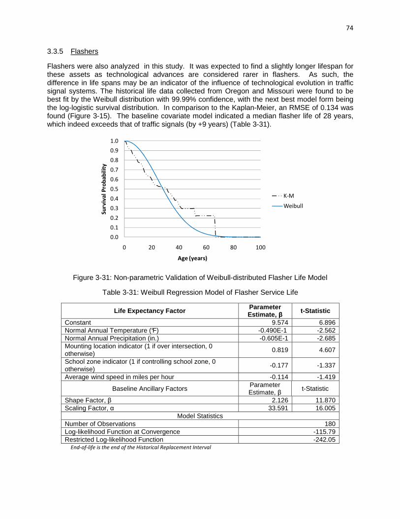
74
3.3.5 Flashers
Flashers were also analyzed in this study. It was expected to find a slightly longer lifespan for these assets as technological advances are considered rarer in flashers. As such, the difference in life spans may be an indicator of the influence of technological evolution in traffic signal systems. The historical life data collected from Oregon and Missouri were found to be best fit by the Weibull distribution with 99.99% confidence, with the next best model form being the log-logistic survival distribution. In comparison to the Kaplan-Meier, an RMSE of 0.134 was found (Figure 3-15). The baseline covariate model indicated a median flasher life of 28 years, which indeed exceeds that of traffic signals (by +9 years) (Table 3-31).
Figure 3-31: Non-parametric Validation of Weibull-distributed Flasher Life Model
Table 3-31: Weibull Regression Model of Flasher Service Life
Life Expectancy Factor Parameter Estimate, β t-Statistic
Constant 9.574 6.896 Normal Annual Temperature (°F) -0.490E-1 -2.562 Normal Annual Precipitation (in.) -0.605E-1 -2.685 Mounting location indicator (1 if over intersection, 0 otherwise)
0.819 4.607
School zone indicator (1 if controlling school zone, 0 otherwise)
-0.177 -1.337
Average wind speed in miles per hour -0.114 -1.419
Baseline Ancillary Factors Parameter Estimate, β
t-Statistic
Shape Factor, β 2.126 11.870 Scaling Factor, α 33.591 16.005
Model Statistics Number of Observations 180 Log-likelihood Function at Convergence -115.79 Restricted Log-likelihood Function -242.05
End-of-life is the end of the Historical Replacement Interval
0.0
0.1
0.2
0.3
0.4
0.5
0.6
0.7
0.8
0.9
1.0
0 20 40 60 80 100
Su
rviv
al
Pro
ba
bil
ity
Age (years)
K-M
Weibull

75
Similar to traffic signals, flasher life was found to be significant affected by climate and the mounting location. Flashers serving intersection traffic (i.e., blinking red stop light) were found to have longer service life. Climatic conditions including temperature, precipitation, and wind speed had a negative relationship with historical service life. Also of significance is the more frequent replacement of flashers over school zones; such frequency may be reflective of the criticality and sensitivity of the service area, thus the high priority assigned to assets in such areas.
3.3.6 Roadway Lighting
Of all the assets studied, roadway lighting had the fewest observations available. As such, more data is needed, in the future, to justify the parametric form used to describe service life. Data that was available included historical replacement intervals and basic information regarding the material type and location of Missouri assets.
With the limited data collected, the Weibull distribution was found to be appropriate with 99.99% confidence. The fit to the Kaplan-Meier estimate had a RMSE of 0.168 (Figure 3-16), largely due an abundance of observations over age 75. With expert opinion placing life closer to 30 years, the integrity of the dataset could be enhanced in the future.
Figure 3-16: Non-parametric Validation of Weibull-distributed Roadway Lighting Life Model
The best fitting Weibull regression model, estimated with the maximum likelihood technique, indicates an average life of 100 years (Table 3-31). This estimate far exceeds that of life estimates in the literature, suggesting that additional observations are needed for modeling life.
0.0
0.1
0.2
0.3
0.4
0.5
0.6
0.7
0.8
0.9
1.0
0 25 50 75 100 125 150 175 200
Su
rviv
al
Pro
ba
bil
ity
Age (years)
K-M
Weibull

76
Table 3-32: Weibull Regression Model of Roadway Lighting Service Life (End-of-life ≡ Historical Replacement Interval)
Life Expectancy Factor Parameter Estimate, β t-Statistic
Constant -4.674 -1.479 Normal Annual Temperature (°F) 0.172 2.933 Material type indicator (1 if metal pole, 0 otherwise) -1.023 -7.964 Mounting location indicator (1 if on sign, 0 otherwise) 1.069 3.113 Functional class indicator (1 if on interstate, 0 otherwise) 0.437 3.440 Fixture height indicator (1 if less than 30 feet, 0 otherwise) -0.350 -1.391
Baseline Ancillary Factors Parameter Estimate, β
t-Statistic
Shape Factor, β 1.764 14.201 Scaling Factor, α 123.609 10.372
Model Statistics Number of Observations 229 Log-likelihood Function at Convergence -177.88 Restricted Log-likelihood Function -328.68
Life expectancy factors that were found to be statistically significant include climate, material type, functional class of roadway, mounting type, and fixture height. Factor levels that were found to be associated with longer life of this asset class include: warmer climates, sign mounting, and interstate service. Tall roadway lighting assets and metal poles tended to have shorter life.
3.3.7 Traffic Signs
The performance of traffic signs can be modeled using an appropriate performance indicator such as the retroreflectivity of the sign sheeting materials (a continuous variable). In addition, a Markov chain can be calibrated to estimate the transition probability of traffic signs progressing from a subjective rating of ‘good’ to ‘fair’ and ultimately ‘poor’. The Markov model in Table 3-32 considers the ‘poor’ stage as the end-of-life condition, while the ‘good’ stage is the initial condition.
Table 3-33. Example transition matrix for simple Markov model of traffic signs
To condition state: From condition state
Good Fair Poor
Good 0.8949 0.1051 0
Fair 0 0.8277 0.1723
Poor 0 0 1.0000
The transition matrix for this asset class was calibrated by optimizing the Markov chain
to a non-linear representation of the average deterioration curve, based on a regression of asset age against condition state. The survival curve in Figure 3-17 suggests that the average life of the traffic signs is about 12 years and that similar signs are unlikely to last beyond 30 years.

77
Figure 3-17. Example Life Expectancy Estimate of Traffic Signs
3.3.8 Pavement Markings
From the literature, it is well established that the life expectancy of pavement markings varies with respect to different factors such as color and marking material type. The following example illustrates the Weibull-distributed survival probability model that was developed on the basis of “1A: 2-year Waterborne yellow markings” data from existing test decks run by National Transportation Product Evaluation Program (NTPEP). The skip-retroreflectivity value of 65 mcd/sq.m/lux was taken as the end-of-life performance threshold.
( )( )βα/0.1exp)( ttS ×−=
where t ≡ the age at which the survival probability is sought, in months. β = shape parameter, 3.87, and the scaling parameter is given by:
α = exp (1.1 – 0.58 * Orientation (1 if longitudinal, 0 if transverse) – 0.01* Initial etroreflectivity value – 0.29 * Road surface type (1 if asphalt, 0 if concrete))
The percentiles of survival distribution can be plotted to give an indication of life expectancy. In this case, the plot suggests that 25% of the markings have a service life of approximately 45 months or more while 75% of the markings have a service life of at least 18 months. On average, the calibrated model indicates an average life of 26 months (Figure 3-18).
The marking performance can also be rated using a discrete subjective rating process which may enable the modeler to apply alternative estimation methods such as Markov chains or ordered probit models. A rating scale may be more appropriate than the current continuous rating based on retroreflectivity only since markings can deteriorate due to various reasons such as abrasion, lack of durability, and lack of contrast.
0.0
0.1
0.2
0.3
0.4
0.5
0.6
0.7
0.8
0.9
1.0
0 10 20 30 40 50 60
Su
rviv
al
Pro
ba
bil
ity
Age in YearsAverage Life 12 yrs

78
Figure 3-18. Example life expectancy estimate of 1A: 2-yr Water-based Yellow Pavement Marking
3.3.9 Pavements
Service Life of New Asphalt Pavements
A non-parametric survival analysis (Kaplan-Meier method) was conducted to estimate the actual probability of survival of a pavement section in relation to pavement age. It was considered that a pavement section has failed when IRI>150. Having chosen this threshold value, the estimated service life represents the age at which a new pavement section will need rehabilitation for the first time. The survival curve of the GPS-1 pavement sections is shown in Figure 3-19. It can be seen that the average service life of new asphalt pavement is approximately 25 years.
Figure 3-19. Survival Curve (Kaplan-Meier method) for hot-mix asphalt concrete pavements
Durat i on
. 20
. 40
. 60
. 80
1. 00
. 005 10 15 20 25 30 35 400
Est i mat ed Survi val Funct i on f or LTI ME
Surv
ival
0
0.1
0.2
0.3
0.4
0.5
0.6
0.7
0.8
0.9
1
0 5 10 15 20 25 30 35 40 45
Pro
ba
bil
ity
of
Su
rviv
al
Age (years)
Average Life 26 months

79
Service Life of Rehabilitation Treatments
An age-based model was developed to determine service life of different rehabilitation techniques as found in LTPP SPS-5 study. The number of observations is 493 and the resulting model is:
ln(IRI)= 0.035 + 0.049*(AGE) – 0.12*(LTHICK) – 0.19*(SPREP); R2=0.52
Where: ln(IRI) = the natural log of IRI of a treated pavement section in given year in m/km; AGE = Time elapsed since rehab treatments, in years; LTHICK = Indicator variable for thickness of rehabilitation treatment (1 if 5 inches and 0 if 2 inches); SPREP = indicator variable for surface preparation of rehabilitation treatment (1 if intensive and 0 if minimal). Service Life of Functional AC Overlay
Functional AC overlay is a common rehabilitation treatment for AC pavements. The following model was developed using data from interstates in Indiana. The regression model that was found to best describe functional AC overlay performance is:
51.37 2.18 log( _ ) 0.3 10 0.03PRE IRI AGE TRAADT PRECIPIRI e−− + × + × × × + ×= ,
2 0.59R =
Where PRE_IRI =IRI before the implementation of the treatment; AGE = Treatment age; TRAADT = Truck annual average daily traffic; PRECIP= Annual average precipitation
Making AGE the subject of the equation, and assuming that when IRI reaches the threshold value, treatment age can be found which is equal to the treatment service life, tSL.
�3® � ln�¢³¢´µ7 �µ6¶�� � 1.37 � 2.18 · [O��log�l³K¹º¹�� � 0.03 · [O��l³K�¢l�0.3 · 10�» · [O���³[[���
The functional AC overlay average service life can be estimated in years. For instance, using the average values in the model the following result was obtained:
5
ln( ) 1.37 2.18 [log( _ )] 0.03 ( )15.5
0.3 10 ( )Threshold
SL
IRI Avg PRE IRI Avg PRECIPt
Avg TRAADT−
+ − × − ×= =× ×
The functional AC overlay average service life was estimated at 15.5 years. As can be seen in the above equation, the average values of the independent variables are used in order to estimate the average service life.
Service life of resurfacing treatment on flexible pavement
Data from Washington State were used to model the performance of resurfacing treatment on flexible pavements. The performance indicator, International Roughness Index (IRI) was used to categorize the pavements into 5 groups – ‘very good’ (5) for IRI=<60, ‘good’ (4) for 60<IRI<94, ‘fair’ (3) for 94<IRI<170, ‘mediocre’ (2) for 170<IRI<220, and ‘poor’ for IRI=>220. The end-of-life criterion was considered to be the state when IRI equals 220. A simple Markov chain model was developed, with a transition matrix as shown in Table 3-33. It was calibrated according to the average deterioration curve, a quadratic curve of the average ages in each condition state.

80
Table 3-34. Markov model of pavement resurfacing
To condition state: From condition state
5 4 3 2 1
5 0.8176 0.1824 0 0 0 4 0 0.7408 0.2592 0 0 3 0 0 0.6230 0.3770 0
2 0 0 0 0.4361 0.5639 1 0 0 0 0 1.0000
The resulting survival curve in Figure 3-20 suggests that the resurfaced pavements have a median life of 12 years.
Figure 3-20. Example life expectancy estimate of pavements treated with resurfacing
3.4 Summary of Life Expectancy Estimates Calibrated to Collected Data
In demonstrating the methodologies presented in the previous chapter, numerical examples for predicting life were provided by defining end-of-life, selecting an age-based, condition-based, or hybrid-based approach, and applying an appropriate modeling technique. The end-of-life definitions used in this chapter varied between actual, observed life and the time until a threshold was triggered for some measure of performance or condition. The approach used to estimate life coincided with the end-of-life definition. When only historical replacement interval data was available, the age-based approach was used; when condition data was available both a hybrid-based approach (Weibull or Log-logistic regression) and a condition-based approach (Markov/Weibull or Markov/Beta) was used. Of the modeling techniques, emphasis was placed on probabilistic estimates produced from Weibull or Log-logistic regression and Markov/Weibull or Markov/Beta models. The use of such techniques were justified through a study of past research, comparing model fit statistics, and assessing the error between the estimated model and non-parametric estimates. The covariate, Weibull and Log-logistic regression approach allowed for the identification of significant life expectancy factors and the ability to further refine life predictions based on disaggregate data. The non-covariate, Weibull/Markov and Weibull/Beta approaches allowed for the comparison of multiple ‘failure mechanisms’ and the
0.0
0.1
0.2
0.3
0.4
0.5
0.6
0.7
0.8
0.9
1.0
0 10 20 30 40 50
Su
rviv
al
Pro
ba
bil
ity
Age in YearsAverage Life 12 years

81
flexibility of comparing different end-of-life thresholds and updating predictions based on current conditions.
To summarize the predictions, the baseline, average service lives and 90% confidence levels from the developed models are presented in Table 3-34. The model factors and statistic are summarized in Table 3-35. Considering the case-by-case nature of the Markov/Beta models, the corresponding parameters are not presented. From the model calibrations, several significant factors were identified, generally including: climatic conditions, soil properties, asset geometrics, functional class characteristics, and maintenance responsibility. In comparing this list to the literature, additional factors that were unavailable at the time of analysis but should be assessed include the repair history (frequency and intensity), construction quality, and deicing chemical applications. In comparing ‘failure mechanisms’, it was seen that element condition ratings generally are the predominant rationale for replacement, excluding extreme events and rationale not modeled. For bridges, besides deck replacements, the substructure was found to be the dominating condition-based rationale.
By following the methodologies and applying the techniques described in the previous chapter, similar analyses can be carried out by agencies to better predict the behavior of their population of assets. Before discussing the uncertainty in such models, the following chapter will discuss how life expectancy predictions can be applied in common business practices. Primarily the estimation of life is useful for assessing life-cycle costs which can be used to evaluate various policies and design selections.
Table 3-34: Summary of Asset Service Life Model Predictions
Asset Class End-of-Life Definition Median Life (years) 90% C.I.
Bridges
Sufficiency Rating ≤ 50% 60 [22, 105] Deck Rating ≤ 5 42 [15,75] Superstructure Rating ≤ 4 64 [27,104] Substructure Rating ≤ 4 59 [23,100] Deck Geometry Rating ≤ 3 >120 N/A Channel Protection Rating ≤ 4 81 [31,139] Scour Protection Rating ≤ 2 >120 N/A
Box Culverts
Historical Replacement Interval or Culvert Rating ≤ 3
55 [21,94]
Culvert Condition Rating ≤ 4 85 [43,125] Channel Protection Rating ≤ 4 88 [30,161]
Pipe Culverts Physical or Structural Rating =3, Flow Rating = 2, or Roadway Deflection ≥ 1 inch
30 [3,317]
Traffic Signals Historical Replacement Interval 19 [3,116] Flashers Historical Replacement Interval 28 [8,56] Roadway Lighting Historical Replacement Interval 100 [23,230] Traffic Signs Condition Rating = ‘Poor’ 12 N/A Pavement Markings (1A: 2-yr water based yellow)
Retroreflectivity < 65 mcd/sq.m/lux 2.17 N/A
Pavement (New construction)
IRI Threshold = 150 in/mile 24 N/A
Pavement (AC Overlay) IRI Threshold = 100 in/mile 15.5 N/A

82
Table 3-35: Summary of Asset Life Model Statistics
Asset Class End-of-Life Definition RMSE* Model
Type Survival Factors
Bridges
Sufficiency Rating ≤ 50% 0.034 Weibull α = 68.87 β = 2.62
Deck Rating ≤ 5 0.986 Markov/ Weibull
α = 48.62 β = 2.50
Superstructure Rating ≤ 4 0.757 Markov/ Weibull
α = 72.26 β = 3.02
Substructure Rating ≤ 4 1.211 Markov/ Weibull
α = 67.36 β = 2.77
Channel Protection Rating ≤ 4 0.847 Markov/ Weibull
α = 92.77 β = 2.70
Box Culverts
Historical Replacement Interval or Culvert Rating ≤ 3
0.096 Weibull α = 63.21 β = 2.73
Culvert Condition Rating ≤ 4 3.683 Markov/ Weibull
α = 93.69 β = 3.77
Channel Protection Rating ≤ 4 3.204 Markov/ Weibull
α = 102.40 β = 2.42
Pipe Culverts
Physical or Structural Rating = 3, Flow Rating = 2, or Deflection ≥ 1“
0.234 Log-Logistic
α = 30.41 β = 1.26
Traffic Signals
Historical Replacement Interval 0.046 Log-Logistic
α = 19.18 β = 1.63
Flashers Historical Replacement Interval 0.134 Weibull α = 33.59 β = 2.13
Roadway Lighting
Historical Replacement Interval 0.168 Weibull α = 123.61 β = 1.76
*RMSE refers to relative fit to Kaplan-Meier estimates for Survival Regression Models and to Markov estimates for Markov/Weibull Models

83
CHAPTER 4 – INCORPORATING LIFE EXPECTANCY ESTIMATES INTO ASSET MANAGEMENT FUNCTIONS
4.1 Fundamental Life Expectancy Applications
Life expectancy estimates are important for the evaluating, ranking, valuing, and budgeting of asset replacement and life extending maintenance/preservation activities. This chapter discusses the issues associated with such decisions and presents a number of numerical examples to show how the life expectancy estimates could be applied in the practice. The Guidebook that accompanies this report describes the contexts of the related asset management decision-making process at highway agencies and also provides an extended range of demonstrations on how asset life expectancy estimates could be incorporated into asset management functions.
4.1.1 Evaluating Replacement and Life Extension Activities Using LCCA
Life Cycle Cost Analysis (LCCA) allows for the economic-based evaluation of competing alternatives over an analysis period, in consideration of monetized benefits and costs (AASHTO, 1993). For LCCA to be appropriate to a given problem at hand, the analysis period is typically equivalent to the life expectancy of the asset. In the asset management task of preservation treatment or strategy identification, the strategy that minimizes life cycle costs (over the asset life cycle) at a specified level of benefits or maximizing life cycle benefits under given cost constraints, or maximizes some function of life cycle benefits and costs under benefit and/or cost constraints, is deemed the optimal treatment or strategy.
4.1.1.1 Brief History of LCCA
The Federal Highway Administration (FHWA) has championed the use of LCCA in analyzing major investment decisions where such analyses are likely to increase the efficiency and effectiveness of investment decisions (FHWA, 1994; FHWA, 1996; FHWA, 2002). As such, recent legislation has required the use of life-cycle costing in highway design, engineering, and management (FHWA, 1998):
• 1991 Intermodal Surface Transportation Efficiency Act (ISTEA 1991) - required the consideration of life-cycle costing in highway design and engineering;
• 1995 National Highway System Designation Act (NHS Act of 1995) - required states to conduct LCCA and Value Engineering Analysis on NHS projects whose costs exceeded a certain threshold; and
• 1998 Transportation Equity Act for the 21st Century (TEA-21) - removed LCCA requirements established in the NHS Act of 1995 but required the development of LCCA procedures on NHS projects.
To aid in the management of infrastructure assets, the Governmental Accounting Standards Board (GASB) released a statement (GASB 34) which established new financial reporting requirements so as to ensure the appropriate use of public resources and allow for increased operational accountability (GASB, 1999). Furthermore, domestic and international studies have found that cost-effective long-term investment decisions in highway asset

84
management could be made at lower costs if LCCA were adopted properly (Al-Mansour & Sinha, 1994).
The following subsections detail life-cycle techniques with an emphasis on the benefits and applications of increased knowledge concerning asset life expectancy. Both LCCA of new and in-service assets is discussed. Numerical examples of how to incorporate life expectancies into LCCA to enhance operational, tactical, and strategic management functions are provided in subsection 4.2.1.
4.1.1.2 LCCA Analysis Period and Asset Life Expectancy Relationship
Past research has shown that the validity of economic decisions is hinged upon the sufficient length of the selected analysis period (Walls III & Smith, 1998). While incremental changes beyond a sufficient length have been found inconsequential (Walls III & Smith, 1998), the life expectancy estimate allows for a proper basis for the period selection.
The analysis period (also known as the planning horizon, planning period, or payment period) is the timeframe over which economic costs and benefits are compared. This length is typically expressed in years and varies depending on whether an agency is considering an existing or proposed asset and can be either less than, equal to, or more than the asset service life. For a new or proposed asset, the analysis period is often taken with respect to the overall life expectancy of the asset; for an existing asset, the analysis period is often taken as the remaining fraction of life (Figure 4-1). The LCCA is then classified as a full-life LCCA for the former case and a partial-life or remaining-life LCCA for the latter.
The analysis period for LCCA can be set as less than, equal to, or more than the life expectancy estimate (Figure 4-2 and Figure 4-3). The former case (Analysis period < life expectancy) is used for the evaluation of short-term or medium term impacts of some intervention. A more valid comparison would be to compare the economic costs and benefits over the entire life expectancy, so as to weigh both construction and replacement costs. For agencies that do not replace the asset at the culmination of service life, a residual period can be included in the analysis period.
In subsequent sections and chapters of this report, the term analysis period is used synonymously with service life.

85
Figure 4-1: Analysis Period for Existing and New Assets
Asset
Performance
Time or Asset Age
Years already elapsed
Scenario 2:
New or Proposed Asset
Asset
Performance
Time or
Asset Age
Performance
Threshold
Analysis Period ≈ Remaining
Life of the Asset
Scenario 1:
Existing Asset
“Current”
Time
Overall Asset Life
“Current” Time
Performance
Threshold
Analysis Period ≈ Overall Life
of the Asset

86
Figure 4-2: Scenarios for Analysis Period Length relative to Overall Life, New Assets
Asset
Performance
Time or
Asset Age
Performance
Threshold
Analysis Period
Asset Life Expectancy
Scenario 1:
Analysis period is less
than the life expectancy
Asset
Performance
Time or Asset Age
Performance
Threshold
Analysis Period = Asset
Life Expectancy
Scenario 2:
Analysis period is equal to the life expectancy
Asset
Performance
Time or Asset Age
Performance
Threshold
Analysis Period
Asset Life Expectancy
Scenario 3:
Analysis period exceeds the life expectancy

87
Figure 4-3: Scenarios for Analysis Period Length relative to Remaining Life, Existing Assets
Asset
Performance
Time or
Years already elapsed
Analysis Period
“Current”
Time
Overall Asset Life
Performance
Threshold
Scenario 1:
Analysis period is less
Asset
Performance
Time or
Years already elapsed
Analysis Period =
Remaining Life of the Asset
Overall Asset Life
Performance
Threshold
Scenario 2:
Analysis period is equal
Remaining Life of the Asset
“Current”
Time
Asset
Performance
Time or
Years already elapsed
Analysis Period Overall Asset Life
Performance
Threshold
Scenario 3:
Analysis period exceeds
the remaining life
Remaining Life of the Asset

88
4.1.1.3 Basic LCCA Concepts
The fundamental interest formulae (also known as equivalence equations) that drive LCCA are used to transform amounts or series of amounts of money from one time period to another in due cognizance of the time value of money. Five variables are related in these formulae (Appendix D): an “initial” amount, a “future” amount, a “periodic” (typically annual) amount, an effective interest rate, and an analysis period. As discussed in the previous subsection, the life expectancy estimate can be used as an effective analysis period. To compare alternatives, seven methods using the interest formulae are used as follows.
(a) Present Worth of Costs (PWC)
This method is used when comparing alternative preservation options with equivalent service life (or lowest common multiple of life) and benefits. The approach converts all costs into an equivalent single cost assumed to occur at the beginning of the analysis period.
(b) Net Present Value (NPV)
To account for the present worth of benefits, the NPV method is used. The NPV represents the present worth of benefits less the present worth of costs. As with the PWC, the NPV reflects the value of the asset preservation option at the time of the base year of the analysis and can be used to compare alternatives with equivalent analysis periods. Of the competing highway asset preservation alternatives, that with the highest NPV is considered the most economically efficient.
(c) Equivalent Uniform Annual Cost (EUAC)
The EUAC method converts all initial and life-cycle costs into an equivalent annual cost over the analysis period. As such, this method is useful for comparing asset preservation options with different service lives but the same levels of benefits.
(d) Equivalent Uniform Annual Return (EUAR)
Similar to NPV, the EUAR method combines all costs and benefits or returns associated with a highway asset preservation option into a single annual value of return (benefits less costs) over a given analysis period. This method can be used when the alternatives have different life expectancies.
(e) Internal Rate of Return (IRR)
Another measure commonly used to justify investment is that of IRR. This method compares the net rate of return [interest rate at NPV equilibration point (i.e., NPV = 0 due to PWB = PWC)] against the minimum attractive rate of return (MARR). If the IRR exceeds the MARR, then a sufficient net profit is anticipated by the end of the analysis period.
(f) Benefit-Cost Ratio Method (BCR)
The benefit-cost ratio (BCR) is a ratio of the NPV or EUAR of all benefits to that of all costs incurred over the analysis period. A preservation option with a BCR exceeding 1 is considered to be economically feasible, and the alternative with the highest BCR value is considered the best alternative.
(g) Incremental Benefit-Cost Ratio Method

89
Similar to the BCR method, the incremental approach relies on a pairwise comparison between alternatives. That is if the following ratio is greater than 0 then alternative x is preferred, else alternative y is preferred.
°} � °¼�} � �¼
Any of the LCCA methods can be used to evaluate the economic efficiency of alternatives.
Another concept in LCCA is the consideration of highway infrastructure that are continuously being reconstructed, as soon as a replacement rationale has been triggered. For such assets, life-cycle costs can be evaluated in perpetuity. For example, the present worth in perpetuity can be evaluated through a single compounded amount R based on a recurring service life of N using the following formula (Sinha & Labi, 2007):
The perpetual life-cycle, however, assumes a recurring service life period (Figure 4-4). In reality, the service life can be variable due to inherent randomness in life expectancy as well as changing environments in terms of climate, design advances, technological developments etc..
Figure 4-4: Perpetual Life-cycle Profile for a Typical Highway Asset
4.1.1.4 Life Expectancy Applications in LCCA
The applications of life expectancy estimates into life-cycle cost analysis can be categorized as operational, tactical, or strategic, with increasing degrees of sophistication. Operational applications refer to the use of an asset life expectancy value to carry out fundamental calculations via the interest formulae. For instance, the calculation of annual costs of new or in-service assets. Tactical applications, which draw upon the results of operational applications, refer to the use of asset life expectancy values to establish life-cycle profiles at the project-level for comparing various strategies. Strategic decisions can then be made based on such applications, examples include:
- Life-cycle Scheduling, Programming, and Budgeting o Trade-off analysis between user cost and asset service life vs. agency
expenditure (Wu & Flintsch, 2009).
- Life-cycle Assessment of Innovations in Asset Management
R
0 N 2N 3Nn* =
Rn*
=
R R
4N N1 N3 N4
Infinity
P’
N2 N1=N2=N3=N4...= N∞
1)1('
−++=
Ni
RP...
)1()1()1('
32, ++
++
++
+=∞ NNNR i
R
i
R
i
RPPW

90
o Life-cycle analysis of the longevity and cost-effectiveness of bridge decks constructed using stainless steel, FRP etc. (Xi et al., 2004; Cope, 2009);
o Cost-effectiveness of warranty contracts on the basis of product life (Shober et al., 1996; Singh et al., 2007).
- Timing of Specific Treatments for Asset Preservation o Quantifying the consequences of delayed or hastened asset preservation actions
(Sharaf et al., 1988; Bilal et al., 2010).
- Life-cycle Impacts of Rehabilitation and Maintenance Treatments o Assessing the service life of asset preservation treatments (Lemer, 1996; Migletz
et al., 2001; Gharaibeh & Darter, 2003; Labi & Sinha, 2003; Lamptey et al., 2005; Labi et al., 2006; Ong et al., 2010);
o Ratio of effectiveness (service life) to cost, for individual alternative preservation treatments (Morian et al., 2003; Irfan et al., 2009);
o Establishing the effectiveness of the asset in terms of the average performance over its service life or the area bounded by the asset’s performance curve (Labi et al., 2006). Both these measures of effectiveness are derived on the basis of the increase in asset life expectancy due to the intervention;
o Quantifying the effectiveness (and given the cost model, the cost-effectiveness) of an intervention that the asset receives.
Strategic applications draw on the results of tactical applications to make high level decisions which include:
- Establishing the optimal application threshold for individual asset preservation treatments (Bilal et al., 2010; Pasupathy et al., 2007);
- Determining the feasibility of a given preservation treatment, material type, etc.; - Identifying the most cost-effective treatment to apply to the asset at a given time; - Identifying optimal rehabilitation & maintenance treatment types and timings over asset
life cycle (Abaza, 2002; Markow & Balta, 1985; Tsunokawa & Schofer, 1994); - Ranking/prioritizing the selection of assets that are most deserving of some preservation
action at a given year and within budgetary constraints.
In addition to assigning an economic worth to alternatives, life expectancy estimates can be used for financial accounting.
4.1.2 Asset Valuation Based on Asset Life Expectancy
Transportation asset valuation is an area of financial accounting that takes into account the depreciating worth of a deteriorating asset with a finite lifespan (Johnson, 2003; Baladi, 2006; Dojutrek, 2011). Techniques commonly applied to estimating the book value of an asset include straight-line and sum-of-years depreciation. These techniques take into account the service life of the asset along with a cost value (construction cost, replacement cost, worth-as-is, and discounted (willing-to-pay):
��£MW��� � �W]� ���£�iWM�Wx] � [99�� �x9� � �M�OM�� ½M�¥���£OWi� -W<�

91
�¥¤ � x< � ¾�M£9 ���£�iWM�Wx] � �[99�� �x9� � �M�OM�� ½M�¥�� 2 ³�¤MW]W]� ��£OWi� -W<�∑ [���3 7��� ®�L �_`
Considering that assets may survive beyond the estimated service life, an alternative valuation technique may be applied. For instance, by using the survival curve, the asset value can be evaluated using: [99�� ½M�¥� � [99�� �x9� 2 ����. Such values can be updated based on the programming of asset maintenance, preservation, or replacement projects.
4.1.3 Ranking Replacement and Life Extension Activities Using Utility Theory
When dealing with multiple attributes, and particularly non-monetary performance measures, the application of utility functions is one technique for ranking investment priorities. Utility is typically defined as a unitless, measure of ‘happiness’ or ‘satisfaction’. Past studies have sought to develop utility curves for a variety of measures including the general areas of agency cost, user cost, mobility, safety, environment, condition, and remaining service life (Li & Sinha, 2004; Sinha et al., 2009). Of interest in this study, is the utility of remaining life which has been developed using expert opinion for all assets (Figure 4-5) as well as that for bridges (Figure 4-6).
� � 1.1659 2 �1 � Kql��0.0195 2 ³�-!��
Figure 4-5: General Remaining Service Life Utility Curve (Li & Sinha, 2004)
0
0.1
0.2
0.3
0.4
0.5
0.6
0.7
0.8
0.9
1
0 2 4 6 8 10
Uti
lity
Remaining Service Life in Years

92
W< ³�- À 5, � � 0
W< 5 Á ³�- Á 15, � � 0.1 2 ³�- � 0.5, ��9�, � � 1
Figure 4-6: Bridge Remaining Service Life Utility Curve (Sinha et al., 2009)
From the two presented utility curves, it can be seen that utility has been assigned a generally, linear relationship has been assigned to remaining service life (RSL), with a lack of concern over structures with a RSL over 15 years (beyond most programming horizons). As such, assets with a low predicted RSL will have the highest priority when it comes to replacement projects. However, as discussed in the next chapter, if the RSL is uncertain, then consequently the utility and ranking will be uncertain as well. The selection of ranked projects, however, is constrained to the available budget, which is in itself related to life expectancies.
4.1.4 Budgeting for Asset Replacement
In budgeting, agencies seek to compare anticipated financial needs over a planning horizon against projected funds. The length of the planning horizon can vary based on the length of the improvement plan, typically 3, 5, or 10 years, or incorporated into more long-term planning, typically 25 years. While many agencies are in a state of ‘worst-first’ activity planning, long-term life expectancy forecasts can be used to minimize life-cycle costs and identify needs prior to there being a potential shortage of funds. If replacement is the most viable option for an asset within the planning horizon, then the replacement cost directly contributes to the budget needs. The summation of replacement costs for all such assets are then used to assess the needed budget for replacement projects.
To demonstrate the use of life expectancy into the various business applications, the following section will provide sample calculations.
0
0.1
0.2
0.3
0.4
0.5
0.6
0.7
0.8
0.9
1
0 5 10 15 20
Uti
lity
Remaining Service Life in Years

93
4.2 Example Calculations Involving Asset Life Expectancy
In demonstration of the business applications, numerical examples of life-cycle cost analysis, ranking projects by utility, and budgeting over various planning horizons are presented in the following subsections.
4.2.1 LCCA Calculations Involving Asset Life Expectancy
The basic concepts of economic analysis, as discussed in preceding sections, form a basis for carrying out LCCA-based evaluation of alternative actions to preserve existing or new highway assets. In this subsection, various applications that may benefit highway agencies are presented from basic calculations of LCCA measures to comparing alternative preservation activities, justifying routine preventative maintenance, identifying the optimal replacement interval, comparing design alternatives, comparing life extension alternatives, pricing design and preservation activities, synchronizing replacements, and assessing the value of life expectancy information [note: presented LCCA examples are adapted from Thompson et al., (2011)].
4.2.1.1 Example Calculations of Basic LCCA Measures
Standard economic texts provide formulae (Appendix D) for basic calculations in engineering economics that serve as the basis for life-cycle cost analysis. In engineering economic analysis, six essential cases can be assessed (note inflation is assumed to be accounted for):
Case 1: Finding the future amount (F) corresponding to a certain initial amount (P) at the end of a given analysis period.
For example, assume it has been estimated from life expectancy models that the remaining service life of a certain large road sign is 5 years. The current price is $20,000. The equivalent cost of replacement when that activity is due can be calculated using the SPCAF, (1+ i)N, where N is the analysis period (in this case, the remaining service life = 5 years). Assume a 5% interest rate, F = P [(1+ i)N] = 20,000[(1+ 0.05)5] = 25,526. The cost of replacement 5 years from now, is then $25,526.
Case 2: Finding the initial amount (P) that would yield a future amount (F) at the end of a given period.
For example, five years from now (2010), a certain highway agency has determined that a certain box culvert will reach the end of its service life and will need to be replaced at an estimated cost of $50,000 at that year. How much should the firm put away now in order to be able to pay for the culvert replacement in 2016? Using the Single Payment Present Worth Factor (SPPWF) and assuming a 5% interest rate, P = F/(1+i)N = 50,000/(1+0.05)5 = 39,176. Therefore, the firm should set aside $39,176 now in order to be able to construct the box culvert 5 years from now (in 2015).
Case 3: Finding the amount of uniform annual payments (A) that would yield a certain future amount (F) at the end of a given period.
If, in case 2, the highway agency is setting aside uniform amounts every year to construct the box culvert when it is due for constructed in 2016 at a cost of $50,000 at that year.

94
The amount that needs to be set aside annually can be calculated using the Sinking Fund Deposit Factor (SFDF) in other words, we seek A given F. Assuming a 5% interest rate, A = F{i/[(1+i)N -1]} = 50,000{0.05/[(1+0.05)5 - 1]} = 9,049. Therefore, the agency should set aside $9,049 each year from now in order to be able to finance the construction of the culvert in 2015.
Case 4: Finding the final compounded amount (F) at the end of a given period due to uniform annual payments (A).
Results of life expectancy modeling suggest that the street light system on a certain city’s main street is due for replacement 8 years from now. The city engineer’s office has in place a revenue generation scheme that provides $9,000 per year. The engineer’s office seeks to ascertain the amount to be generated when the street lights are due for replacement. This is a Uniform Series Compounded Amount Factor (USCAF) problem: we seek F given A. Assume a 5% interest rate, F = A{[(1+i)N -1]/i} = 9,000{[(1+0.05)8 - 1]/0.05} = 85,942. Therefore, at the end of the service life of street lights, the local agency would have raised $85,942.
Case 5: Finding the initial amount (P) that is equivalent to specified uniform future amounts (A) over a given analysis period.
For example, a certain highway agency seeks how much to set aside at the current time (say, year 2010), that would be equivalent to $2,100 annual amounts for routine maintenance of its road flasher assets over the remaining 12 years of their service life. Assume that all the flashers in question were installed at the same year. This is a Uniform Series Present Worth Factor (USPWF) problem: we seek P given A. Assume 4% interest rate, P = A{[(1+i)N -1]/[i(1+i)N]} = 2,100{[(1+0.04)12 -1]/[0.04(1+0.04)12]} = 19,709. Therefore, $19,709 needs to be procured at the current time to yield the required annual maintenance amount over the remaining service life of the road flasher assets.
Case 6: Finding the amount uniform annual payments (A) over a given period, that is equivalent to an initial amount (P).
A state highway agency seeks to finance the replacement of its aging road signs that were constructed in the early seventies. In December 2010, the agency receives a loan of $200,000 to carry out the project, to be repaid over a 10-year period. From life expectancy models, the expected service life of the new assets is 10years. How much will the agency need to pay back to the bank every year (starting December 2011) until December 2021? It may be noted here that in this particular example, the analysis period is less than the life expectancy of the new asset. This is a Uniform Series Capital Recovery Factor (USCRF) problem. In other words, we seek A given P. Assume 3% interest rate, A = P{[i(1+i)N]/[(1+i)N -1] } = 200,000{[0.03(1+0.03)10]/[(1+0.03)10 -1]} = 23,446. Therefore, $23,446 needs to be paid back every year.
4.2.1.2 Example LCCA Calculations for Comparing Alternative Preservation Activities
As described previously, seven methods of evaluating life-cycle costs can be applied. Examples of each relating to asset life expectancy are provided.
(a) Present Worth of Costs (PWC)

95
For example, consider a bridge replacement is proposed by an agency. The initial cost of design type A is $50M, average annual maintenance cost is $0.25M, and the bridge has a salvage value of $8M. For design type B, the initial cost is $30M, average annual maintenance cost is $0.75M, and salvage value is $2M. From life expectancy model, it has been determined that both designs have a useful life of 75 years. The present worth of design A, PWCA (in millions) = 50 + 0.25× USPWF(7%, 75) – 8× SPPWF(7%, 75) = $53.50M. PWCB (in millions) = 30 + 0.75× USPWF(7%, 75) – 2× SPPWF(7%, 75) = $40.63M. Thus, Alternative B is more economically attractive, from a life-cycle viewpoint.
(b) Net Present Value (NPV)
For example, in the problem in (c), the net present value for each alternative can be determined as follows, using the lowest common multiple (35 years) as the analysis period (see section 3.3.2 for a discussion of analyzing assets with different service lives):
NPVA (in millions) = (0.07 – 0.08)× USCRF(4%, 35) – 2× [1 + SPPWF(4%, 5) + SPPWF(4%,10) + ... SPPWF(4%,35) = -$9.08M
NPVB (in millions) = (0.05 – 0.09)× USCRF(4%, 35) – 1.75× [1 + SPPWF(4%, 3.5) + SPPWF(4%,7) + ... SPPWF(4%,35) = -$11.38M
Thus, Alternative A is more desirable [confirming the result in (c)].
(c) Equivalent Uniform Annual Cost (EUAC)
For example, consider a case where road lighting can be provided satisfactorily using any one of two alternative pole types, A or B that differ in both material and design configuration. Type A has an initial cost of $10,000, annual maintenance and operating costs of $800 and $2,000 salvage value. Type B has an initial cost of $7,500, annual maintenance and operating costs of $1,200 and $1,000 salvage value. From life expectancy modeling, the estimated remaining service lives of the pole types A and B are 16 and 12 years, respectively. Assuming a 6% interest rate, the EUAC of each alternative is calculated as follows:
EUAC of Alternative A (in thousands) = 10× USCRF(6%, 16) + 0.8 – 2× SFDF(6%, 16) = $1.71k
EUAC for Alternative B (in thousands) = 7.5× CRF(6%, 12) + 1.2 – 1× SFDF(6%, 12) = $2.04k
Clearly, Alternative A is more desirable, from the life-cycle cost viewpoint.
(d) Equivalent Uniform Annual Return (EUAR)
For example, two alternative materials are being considered for road pavement markings at Interstate highway 999. Alternative A involves an initial project cost of $2M, an estimated design life of 5 years, annual maintenance costs of $0.08M, and $0.07M worth of annual benefits in terms of monetized savings due to enhanced safety. Assume that both alternatives will yield similar levels of performance and have no salvage value. Alternative B has an initial project cost of $1.75M, an estimated life of 3.5 years, annual maintenance and operating costs of $0.09M, and $0.05M worth of annual benefits in terms of safety enhancement. The agency can identify the superior alternative as follows: Assume a 4% interest rate.
EUARA (in millions) = 0.07 – [2 *USCRF(4%,5) + 0.08] = -$0.46M
EUARB (in millions) = 0.05 – [1.75*USCRF (4%,3.5) + 0.05] = -$0.66M

96
Thus, pavement marking material type A is more desirable, from a life-cycle perspective.
(e) Internal Rate of Return (IRR)
For example, a county road agency is considering the construction of a culvert to provide accessibility to a remote area of a certain state. The $30,000 culvert will reduce travel time by eliminating the need for lengthy detours. However, given the acidity of the soil, the estimated life of the culvert is only 40 years, after which time the value of culvert will be $15,000. The expected travel time savings per year is $5,000 per year, and the average annual maintenance cost is $2,000. Is the project economically more desirable? Or should the agency just do nothing? The minimum attractive rate of return is 5%.
Equating the net cash flow on both sides, yields:
5,000× USPWF(i%,40) + 15,000× SPPWF(i%,40) = 30,000 + 2000× USPWF(i%,40)
Solving this equation by trial and error yields: i = 9.88% > 5% so it is economically more efficient to undertake the project than the do-nothing alternative.
(f) Benefit-Cost Ratio Method (BCR)
For the problem in (c), determine the benefit-cost ratio for each alternative.
For Alternative A: Benefits (in millions) = $0.07M
Cost = (in millions) = 2× USCRF(4%, 5) + 0.08 = $0.53M; BCRA = 0.07/0.53 = 0.13
For Alternative B: Benefits (in millions) = $0.05M ; Costs (in millions) = 1.75× USCRF(4%, 3.5) + 0.09 = $0.71M; BCRB = 0.05/0.71 = 0.07
BCRA > BCRB. Thus, Alternative A is more desirable.
(g) Incremental Benefit-Cost Ratio Method
Consider a new subset of alternatives with the following benefits and costs:
Alternative X: Benefits = $2M, Cost = $0.8M;
Alternative Y: Benefits = $3M, Cost = $1.5M;
Alternative Z: Benefits = $9M, Cost = $4M;
Determine the best alternative using the incremental benefit-cost ratio method.
First compare Alternatives X and Y:
°} � °¼�} � �¼ � $2� � $3�$0.8� � $1.5� � 1.43 à [���£]M�WO� q
Next compare Alternatives X and Z:
°} � °Ä�} � �Ä � $2� � $9�$0.8� � $4� � 2.19 à [���£]M�WO� q
The best alternative is therefore alternative X.

97
In addition to evaluating projects with a finite analysis period, agencies can also assess life-cycle costs in perpetuity. For example, consider the following case for a large reinforced box culvert is slated for reconstruction.
Assume a reconstruction cost is $600,000. During its replacement cycle, the culvert will require two rehabilitations, each with a cost of $200,000, at the 20th and 40th year, and the average annual cost of maintenance is $5,000. From life expectancy models, the estimated service life is 60 years. At the end of the replacement cycle, the bridge will again be reconstructed and the entire cycle is assumed to repeat in perpetuity. Find the capitalized costs to perpetuity. Assume 5% interest rate. Assume P’ (the starting non-recurring cost = 0)
The compounded life-cycle cost, R, is determined as follows: 600,000SPCAF(5%, 60) + 200,000SPCAF(5%, 40) + 200,000SPCAF(5%, 20) + 5,000USCAF(5%, 60) = $14,914,087.
Then the present worth of R, taken to perpetuity, is:
lJ∞ � ³�1 � W�¡ � 1 � $14,914,087�1 � 0.05�ÆQ � 1 � $843,596
4.2.1.3 Example LCCA Calculations for Justifying Routine Preventative Maintenance
A common maintenance planning issue is the question of whether to start routine programs of crew activities that might have life extension benefits. Common examples are sealing of pavement cracks; washing of bridges, signs, pavements, and guiderails; spot painting of steel structures; and concrete patching. To evaluate the merit of such strategies, consider the following example, which compares a preventive maintenance scenario against the do-nothing scenario.
Through the application of preventative maintenance, the two scenarios will likely have different service lives. For comparing asset alternatives that have different service lives, there are at least three approaches for each alternative: (i) convert all costs and benefits into EUAC, (ii) compute life cycle cost over a service life that is a lowest common denominator of the separate life expectancy estimates, or (iii) find the present worth of periodic payments to perpetuity
Consider, for example, the use of the EUAC approach for comparing the two strategies in a pavement management system (Table ). For the routine preventive maintenance strategy, assume crack sealing is performed every 4 years at $400 per lane-mile resulting in a overall life extension of 4 years; for the do-nothing option, assume only reconstruction is performed at a cost of $30k per lane-mile for both alternatives. Assume an interest rate of 4%.

98
Table 4-1: Example Comparison of Life-Cycle Activity Profiles in Evaluating the Benefit or Disbenefits of Conducting Routine Preventative Maintenance
Cost per lane -mile by strategy Year Routine Preventative
Maintenance Do-Nothing
4 $400 8 $400
12 $400 16 $400 20 $400 $30,000 24 $30,000
The EUAC of the two alternatives can be compared as follows:
l½º6Ç��c È7 � c��� ~"�c� c"c� � $400 @ 1�1 � 0.04�) � 1�1 � 0.04�É � Ê 1�1 � 0.04�!QC � $20,000 @ 1�1 � 0.04�!)C = $12,984/lane-mile
K�[�º6Ç��c È7 � c��� ~"�c� c"c� � $12,984 0.04�1 � 0.04�!)�1 � 0.04�!) � 1�
= $852/lane-mile
K�[�*6�¡6�µ�cË � $30,000 @ 0.04�1 � 0.04�!Q � 1C = $1,007/lane-mile
With these assumptions, the agency could reduce annual costs by $156 per lane-mile if routine preventive maintenance is completed.
4.2.1.4 Example LCCA Calculations for Identifying the Optimal Replacement Interval
Certain types of assets may have a variety of service life alternatives, depending on different strategies for maintenance and life extension. The optimal service life would be the life cycle activity profile that can be sustained at a minimum life cycle cost.
For example, consider the alternative profiles in Table for a railway bridge. Assuming an interest rate of 5%, the present worth of all bridge agency costs in perpetuity are to be compared against. The option that minimizes the present worth at perpetuity is to be selected.

99
Table 4-2: Example Data for Optimizing Replacement and Maintenance Activity Intervals
Option 1 Option 2 Option 3 Option 4
Replacement Cost $600k $600k $600k $600k
Rehabilitation Cost $200k $200k $200k $200k
Annual Maintenance Cost $5k $5k $5k $5k
Estimated Service Life (years)
50 60 70 80
Rehabilitation Year 1 25 25 25 20
Rehabilitation Year 2 40 45 45 40
Rehabilitation Year 3 -- -- 55 60
Option 1 (Rehabilitate at years 25 and 40 � Service Life = 50 years)
lJÌ?��6c ` � $600# @ 1�1 � 0.05�»QC � $200# @ 1�1 � 0.05�!» � 1�1 � 0.05�)QC� $5# �1 � 0.05�»Q � 10.05 2 �1 � 0.05�»Q�
= $231,072
lJ∞Ì?��6c ` � $231,072�1 � 0.05�»Q � 1 � $22,075
Option 2 (Rehabilitate at years 25 and 45 � Service Life = 60 years)
lJÌ?��6c ! � $600# @ 1�1 � 0.05�ÆQC � $200# @ 1�1 � 0.05�!» � 1�1 � 0.05�)»C� $5# �1 � 0.05�ÆQ � 10.05 2 �1 � 0.05�ÆQ�
= $208,088
lJ∞Ì?��6c ! � $208,088�1 � 0.05�ÆQ � 1 � $11,770
Option 3 (Rehabilitate at years 25, 45 and 55 � Service Life = 70 years)
lJÌ?��6c Í � $600# @ 1�1 � 0.05�ÎQC � $200# @ 1�1 � 0.05�!» � 1�1 � 0.05�)» � 1�1 � 0.05�»»C� $5# �1 � 0.05�ÎQ � 10.05 2 �1 � 0.05�ÎQ�
= $197,753
lJ∞Ì?��6c Í � $197,753�1 � 0.05�ÎQ � 1 � $6,720

100
Option 4 (Rehabilitate at years 20, 40 and 60 � Service Life = 80 years)
lJÌ?��6c ) � $600# @ 1�1 � 0.05�ÉQC � $200# @ 1�1 � 0.05�!Q � 1�1 � 0.05�)Q � 1�1 � 0.05�ÆQC� $5# �1 � 0.05�ÉQ � 10.05 2 �1 � 0.05�ÉQ�
= $213,876
lJ∞Ì?��6c ) � $213,876�1 � 0.05�ÉQ � 1 � $4,404
Using the assumed costs, Option 4 was found to minimize life cycle cost in perpetuity. Therefore, it is recommended to pursue rehabilitation activities in years 20, 40, and 60 and replace the structure in year 80.
4.2.1.5 Example LCCA Calculations for Comparing Design Alternatives
Asset managers consistently must choose between competing designs and material types, each with a unique life expectancy. To decide between designs, life-cycle costs can be evaluated. For example, consider the decision of applying a protective coating to a pipe culvert. Suppose that without the coating, the pipe culvert is expected to survive 50 years with a construction cost of $1000. With coating, the pipe culvert that is expected to survive 56 years with a construction cost of $1200. As discussed in section 5.3.1, three possible ways of making this comparison would be an annual cost basis using Equivalent Uniform Annual Cost; a least common multiple analysis period consisting of multiple replacement cycles; or a perpetuity of replacement cycles. For this example, a perpetuity is assumed, with a 4% interest rate. The present value of the two options in perpetuity are:
l½∞c6 �6"��cË � $1,000 · Ï1 � `�`nQ.Q)�Ð�`Ñ = $ 1,164
l½∞�6"��cË � $1,200 · Ï1 � `�`nQ.Q)�ÐÒ�`Ñ = $ 1,350
Therefore, the uncoated design option is preferred.
4.2.1.6 Example LCCA Calculations for Comparing Life Extension Alternatives
Another life expectancy application faced by asset managers, is the need to compare two or more life extension alternatives with different costs and levels of effectiveness. Consider the set of alternatives presented in Table , for a bridge having a service life of 50 years (before maintenance), a replacement cost of $500k, and interest an rate of 4%.

101
Table 4-3: Example Bridge Life Extension Alternatives
Activity Frequency Life Extension of Activity at Applied Frequency
Activity Cost
Deck overlay Every 20 years 7 $15k Deck patching Every year 3 $500 Joint replacement Every year 2 $300 Deck overlay & joint replacement
Overlay every 20 years & joint replacement every year
9 $15k for overlay and $100 for joint
replacement Deck patching & joint replacement
Every year 5 $700
Deck rehabilitation Once at year 35 30 $200k
In a bridge management system, these types of strategies are typically compared on a net present value basis, and more than one of them may be selected. For the current example, EUAC is used as the selection criterion.
EUAC of Deck Overlay � @$15k 2 A 1�1 � 0.04�!Q � 1�1 � 0.04�)QB � $500k 2 A 1�1 � 0.04�»QnÎBC2 0.04�1 � 0.04�»QnÎ
�1 � 0.04�»QnÎ � 1
= $2.84k
EUAC of Deck Patching � $500 � @$500k 2 A 1�1 � 0.04�»QnÍBC 2 0.04�1 � 0.04�»QnÍ�1 � 0.04�»QnÍ � 1
= $3.36k
EUAC of Joint Replacement � $300 � @$500k 2 A 1�1 � 0.04�»Qn!BC 2 0.04�1 � 0.04�»Qn!�1 � 0.04�»Qn! � 1
= $3.29k EUAC of Deck Overlay and Joint Replacement � $100 � @$15k 2 A 1�1 � 0.04�!Q � 1�1 � 0.04�)QB � $500k 2 A 1�1 � 0.04�»QnáBC2 0.04�1 � 0.04�»Qná
�1 � 0.04�»Qná � 1
= $2.74k EUAC of Deck Patching and Joint Replacement � $700 � @$500k 2 A 1�1 � 0.04�»Qn»BC 2 0.04�1 � 0.04�»Qn»
�1 � 0.04�»Qn» � 1
= $3.32k EUAC of Deck Rehabilitation � @$200k 2 A 1�1 � 0.04�Í»B � $500k 2 A 1�1 � 0.04�»QnÍQBC 2 0.04�1 � 0.04�»QnÍQ
�1 � 0.04�»QnÍQ � 1
= $3.32k
EUAC of Do Nothing � $500k 2 A 0.04�1 � 0.04�»Q � 1B
= $3.28k

102
From this array of activity options, the improvement strategy that minimizes cost under these assumptions is annual deck overlay and joint replacement. It can also be seen that the life extensions from patching, joint replacement, and rehabilitation under these assumptions are not cost effective (relative to do-nothing option).
4.2.1.7 Example LCCA Calculations for Pricing Design and Preservation Alternatives
Many agencies invest in research and development programs in an attempt to produce practical, cost effective designs and materials. The primary concern with innovations, however, are the reliability, life extension benefits, and cost of application. To ease decisions on whether to apply a new design, agencies often assess break-even points (point at which an alternative design becomes less costly).
For instance, consider an agency that wishes to assess the feasibility of switching from traditional carbon steel reinforcement bars to solid stainless steel reinforcement bars. If the service lives of these bridges are 75 years and 100 years, respectively, with the activity profiles in Figure 4-7, at what price is the stainless steel alternative preferred? Assume a bridge with initial construction cost (traditional carbon steel) = $200k; rehabilitation cost = $25k; deck replacement cost = $75k.
Figure 4-7: Example Activity Profiles for Carbon Steel and Stainless Steel Options (Cope, 2009)
EUAC of Carbon Steel� @$200k � 25k 2 A 1�1 � 0.04�ÍQ � 1�1 � 0.04�ÆQB � 75k 2 A 1�1 � 0.04�)»BC2 0.04�1 � 0.04�λ
�1 � 0.04�λ � 1
= $9.41k
EUAC of Stainless Steel � @�$200k � �� � 25k 2 A 1�1 � 0.04�»QBC 2 0.04�1 � 0.04�`QQ�1 � 0.04�`QQ � 1
� �$203.5k � �� 2 0.0408
Solving for cost that would equate costs of carbon steel and stainless steel
• Year 0: Initial Construction
• Year 30: Rehabilitation
• Year 45: Deck Replacement
• Year 60: Rehabilitation
• Year 75:End of Service Life
Carbon Steel
• Year 0: Initial Construction
• Year 50: Rehabilitation
• Year 100: End of Service Life
Stainless
Steel

103
$9.41# � �$203.5k � �� 2 0.042 � � $27.2#
Therefore, for an additional construction cost of z ≤ $27.2k, the stainless steel option is preferred.
4.2.1.8 Example LCCA Calculations for Synchronizing Replacements
Maintenance interventions can be costly and disruptive, as such, agencies often wish to synchronize work within a corridor. Therefore, knowledge of the remaining life of all assets in a corridor would assist the manager in timing replacement and/or maintenance activities. For example, consider a small system of assets located along the same roadway (Table 4-4). If the location costs (i.e., mobilization, traffic control, and user costs) are estimated to be $7,000 per construction set-up, then what are the optimal replacement times so as to minimize the present value of costs in perpetuity? Assume assets are to be replaced no later than their remaining service life.
Table 4-4: Example data for synchronizing replacement intervals
Asset New Construction
Service Life
Remaining
Service Life
Replacement Cost
Pavement Markings 5 3 $200
Traffic Sign 10 4 $300
Traffic Signal 15 5 $500
The objective of this problem is to minimize the total life cycle cost, computed as follows:
l½ � \ []]¥M� ³���Mi�¤�]� �x9� 2 A 11 � WBc�c"¶å��� È 7�6�c_`
Where: []]¥M� ³���Mi�¤�]� �x9� � Location Cost 2 ∑ xÍèééêë_` èééêë Replacement Costèééêë; x ≡ binary decision variable indicating replacement, 1=replace, 0=do-nothing; n ≡ year of potential replacement.
The only constraint is that remaining service life must be greater than zero, ³�- ì 0 ∀n.
This optimization problem can be solved using a solver software package, although it is simple enough to solve by inspection, recognizing that an agency would ideally like to coordinate replacements so as to minimize cost and that the new construction service life estimates have a common multiple of 5 years. Therefore, the optimal solution can be seen to be:
• Replace all assets in year 3.
• Replace pavement markings every 5 years thereafter (i.e., years 8, 13, 18, 23, 28, 33).
• Replace traffic signs every 10 years thereafter (i.e., years 13, 23, 33).
• Replace traffic signals every 15 years thereafter (i.e., years 18, 33). This produces the same life-cycle profile every 30 years with a present value of $26k.

104
Alternatively, if an agency did not coordinate replacement schedules, and replaced assets at the time each asset’s full service life is reached:
• Replace pavement markings in year 3 and every 5 years thereafter (i.e., years 3, 8, ... 33).
• Replace traffic signs in year 4 and every 10 years thereafter (i.e., years 4, 14, 24, 34).
• Replace traffic signals in year 5 and every 15 years thereafter (i.e., years 5, 20, 35). Then a common life-cycle profile every 30 years with a present value of $80k is obtained.
This example shows that the strategy of sacrificing 1 year of traffic sign life and 2 years of traffic signal life initially, so as to synchronize replacements, ultimately lowers the present value of costs by $54k ($80k-$26k).
4.2.1.9 Example LCCA Calculations for Assessing the Value of Life Expectancy Information
To justify the development of asset management systems for less studied asset types (i.e., non-bridges and non-pavements), a comparison of expert opinion to statistically-based life expectancy estimates can be used to evaluate the benefits of additional data collection used in model development. For example, suppose a life expectancy model predicts a box culvert life of 60 years. If an asset is 45 years old and expert opinion puts the service life at 50 years, then a replacement project is likely to be programmed within 5 years. However, statistical evidence would suggest this project should not be programmed for another 15 years. The consequences of this can be quantified via life-cycle analysis. Assume the cost of replacement is $100k at an interest rate of 4%.
Remaining EUAC of replacement, as scheduled by expert opinion:
$100k 2 Q.Q)�`nQ.Q)��` = $18.46k
Remaining EUAC of replacement, as scheduled by life expectancy modeling:
$100k 2 Q.Q)�`nQ.Q)�u�` = $4.99k
Based on this analysis, reliance on expert opinion may cost an additional $13.47k over the asset’s life depending on the accuracy of the life expectancy model. Reliable life estimates can benefit agencies in setting financial needs and effectively spending taxpayer funds.
4.2.2 Asset Valuation Based on Asset Life Expectancy
To demonstrate the application of asset valuation techniques, assume an urban, concrete box culvert is to be constructed on a non-NHS, non-interstate roadway maintained by a state agency with the following characteristics and environmental conditions: opening width = 19.2m, structure length = 11.5m, opening area = 5.33m. normal annual temperature = 50.4°F, normal annual precipitation = 39.4 inches, and a soil classified as highly corrosive with a pH above 6.5. Given these conditions, assumption of a cost of $3,770 per lineal square foot given the opening area (Sinha et al., 2009), and the covariate model in a previous section, the asset value as a function of time is projected (Figure 4-8).

105
Figure 4-8: Example Asset Valuation using Highway Asset Life Expectancy
Standard, straight-line depreciation techniques can be seen to underestimate asset value relative to the survival-based depreciation (by $72k at median life estimate). This demonstrates the risk of underestimating asset life and that the current infrastructure system may be more valuable than predicted in considering that half of the assets will survive longer than the deterministic life estimate.
4.2.3 Utility Calculations Involving Asset Life Expectancy
Project selection is often based on the ranking of various alternatives using utility theory. The set of projects that maximizes utility while constrained to a budget, is then programmed. The utility of projects is often in part based on remaining service life estimates, with higher utility associated with longer service life. For example, assume an agency has calculated the utility for a set of projects with respect to life expectancy, deterioration, life cycle cost, and estimated project cost (Table 4-5). Assume a budget of $2.75M.
Table 4-5: Example ranked projects with associated utility and cost
Activity Utility Cost
Bridge A replacement 100 $2400k
Bridge B rehabilitation 75 $250k
Box Culvert A replacement 55 $100k
Pipe Culvert A replacement 35 $5k
Bridge C deck patching 32 $20k
To select a set of projects, optimization techniques can be applied to the problem:
$0
$20,000
$40,000
$60,000
$80,000
$100,000
$120,000
$140,000
0 20 40 60 80 100 120
Ass
et
Val
ue
Age in Years
Sum-of-Years
Survival Based
Straight Line
Life Estimate

106
�M�W¤W�� l£x�£M¤ ��W�W�¾ � \ ����W�W�¾�î�
�¥N;�i� �x l£x�£M¤ �x9� Á \ ���x9��î�
Where: x ≡ binary decision variable with 1 = program, 0 = do not program; m ≡ number of potential projects.
This simple example can be readily solved in Excel for a small sample size. In this case, the optimal solution would be to replace bridge A, rehab bridge B, replace pipe culvert A, and patch bridge C yielding a total utility of 242 at a cost of $2.675M. The remaining $75k could be carried over to the next programming cycle.
4.2.4 Budget Calculations Involving Asset Life Expectancy
The calculation of budget needs is irrespective of utility. For instance, with the data in Table 4-6, a budget of $20k is needed for a 5 year horizon (Bridge C project), $120k is needed for a 10 year planning horizon (Box Culvert A and Bridge C projects), and $2.52M for a 15 year planning horizon (Bridges A and C and Box Culvert A projects).
Table 4-6: Example Needs Assessment Data
Activity RSL Cost Bridge A replacement 15 $2400k Bridge B replacement 30 $250k Box Culvert A replacement 9 $100k Pipe Culvert A replacement 21 $5k Bridge C deck replacement 5 $20k
4.3 Summary of Life Expectancy Applications
As shown in this chapter, life expectancy estimates are critical for the evaluation of alternatives via life-cycle cost, programming of projects via utility, and assessing budget needs. Building on the life expectancy prediction and the business applications, the following chapter will focus on incorporating uncertainty. Primarily, the risk of making less than optimal business decisions based on uncertain asset life is examined.

107
CHAPTER 5 – METHODS TO ACCOUNT FOR ASSET LIFE UNCER TAINTY IN ASSET REPLACEMENT DECISIONS
5.1 Rationale for Incorporating Risk Into Long-term Planning
As shown in the previous chapter, life expectancy estimates are critical for cost-effective asset management. Asset life, however, is an uncertain quantity which can lead to less than optimal decisions. An inaccurate life estimate puts an agency at risk for not having the available funds on-hand to replace the ‘failed’ asset, resulting in inadequate levels of performance, a biased alternative selection, and an errant project prioritization. Risk-informed decisions can allow agencies to compare levels of confidence against costs.
The uncertainty of the life estimate, as listed in a previous section, is a result of (Lin, 1995; Maskey, 1999):
• Modeling Techniques – error created through idealized mathematical modeling attempting to describe complex physical phenomena (e.g., assume normality of errors);
• Inputs – inherent randomness of structural characteristics (e.g., material properties and strength), future loadings (e.g., traffic volume), environmental conditions (e.g., climatic conditions and soil characteristics), and inaccurate inspection data (e.g., visual condition ratings);
• Parameters – inaccurate representation of the contribution of a factor towards asset deterioration processes; and
• Externalities – unforeseen causes that may surmount natural deterioration processes (e.g., extreme weather event, design/construction flaw, or terrorist attack)
In this chapter, two types of propagating uncertainties are examined. First, using the developed covariate models, the uncertainty surrounding future climatic conditions is assessed. In dealing with climate change, researchers have focused on either mitigation or adaptation. The latter of which is examined with respect to adapting towards new asset life expectancies given the uncertain future climate. Specifically with temperature, precipitation, and freeze-thaw cycles found to be significant life expectancy factors, the uncertainty surrounding such values will compound the uncertainty of asset life and consequently planning decisions.
Second, using the non-covariate models, the uncertainty surrounding the ‘failure mechanism’ and overall life is quantified. As a result, the methodology presented will be of use for asset managers to assign confidence levels to typical planning decisions and to prepare mitigation strategies.
Techniques to quantify such uncertainties are detailed in the following section. After which a comprehensive review of risk analysis in transportation is presented. To build on this literature, a methodology and case study assessments of risk are provided.

108
5.2 Overview of Uncertainty Analysis
The two basic methods of assessing uncertainty can be classified as sensitivity (deterministic) analysis or risk (stochastic) assessment, a part of the larger concept of risk analysis. More detailed methodologies of both analysis types are detailed in sections 5.2.8 and 5.2.9, respectively.
Sensitivity (or What if?) analysis generally refers to the analysis of how the output varies given a systematic, typically unit, change in inputs and/or parameters across their respective sets. This analysis is commonly done for one input at a time, however a multivariate sensitivity analysis is possible if the correlation between inputs is relatively known. Alternatively, sensitivity analysis may also encompass the study of how much an input or parameter may change without having an effect on the output.
Instead of systematic changes, a risk assessment can track how the output changes given a random sampling of input and/or parameter values from a distribution. This approach is more commonly applied for random variables that have a known distribution and for dealing with multiple random variables.
Prior to conducting sensitivity analysis or risk assessment, it is first critical to understand the set of potential values that are being varied or sampled.
5.2.1 Describing Values with Set Theory
Sets (i.e., all possible values for a given input, parameter, or output) are typically described using (Isukapalli, 1999; Ayyub & Klir, 2006):
• Classical (Crisp) Set Theory – Set of mutually exclusive values o e.g., set A = {x1, x2, x3}
• Fuzzy Set Theory (Zadeh, 1965) – Set of vague/imprecise values that can have partial membership in various subsets. o e.g., set A = {x1/M(x1), x2/M(x2), x3/M(x3)}
• Rough Set Theory (Pawlak, 1982) – A coarse, interval set of values defined by approximated lower and upper bounds that can be crisp or fuzzy.
o e.g., set A = { [ R (x1), (x1) ], [ R (x2), R (x2) ], [ R (x3), (x3) ] }
A graphical representation of classical (crisp), fuzzy, and rough values is presented in Figure 5-1. For example, if a bridge condition rating is said to be either in one state or another, then the set of condition ratings is classical. If the bridge condition rating is said to be partially in more than one state, then the set is fuzzy. If the bridge condition rating is definitely (crisp) or partially (fuzzy) between one state and another across some range, then a rough set is used.
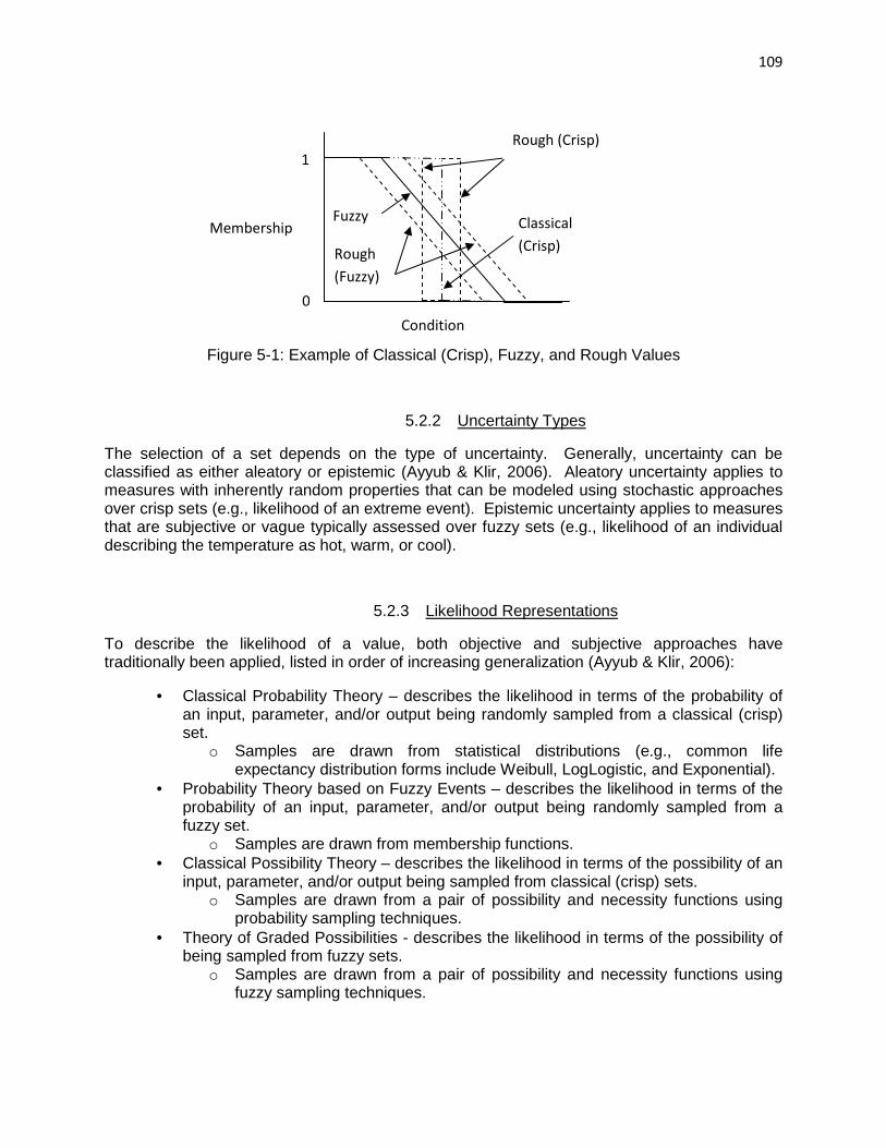
109
Figure 5-1: Example of Classical (Crisp), Fuzzy, and Rough Values
5.2.2 Uncertainty Types
The selection of a set depends on the type of uncertainty. Generally, uncertainty can be classified as either aleatory or epistemic (Ayyub & Klir, 2006). Aleatory uncertainty applies to measures with inherently random properties that can be modeled using stochastic approaches over crisp sets (e.g., likelihood of an extreme event). Epistemic uncertainty applies to measures that are subjective or vague typically assessed over fuzzy sets (e.g., likelihood of an individual describing the temperature as hot, warm, or cool).
5.2.3 Likelihood Representations
To describe the likelihood of a value, both objective and subjective approaches have traditionally been applied, listed in order of increasing generalization (Ayyub & Klir, 2006):
• Classical Probability Theory – describes the likelihood in terms of the probability of an input, parameter, and/or output being randomly sampled from a classical (crisp) set.
o Samples are drawn from statistical distributions (e.g., common life expectancy distribution forms include Weibull, LogLogistic, and Exponential).
• Probability Theory based on Fuzzy Events – describes the likelihood in terms of the probability of an input, parameter, and/or output being randomly sampled from a fuzzy set.
o Samples are drawn from membership functions. • Classical Possibility Theory – describes the likelihood in terms of the possibility of an
input, parameter, and/or output being sampled from classical (crisp) sets. o Samples are drawn from a pair of possibility and necessity functions using
probability sampling techniques. • Theory of Graded Possibilities - describes the likelihood in terms of the possibility of
being sampled from fuzzy sets. o Samples are drawn from a pair of possibility and necessity functions using
fuzzy sampling techniques.
Classical
(Crisp)
Rough (Crisp)
Fuzzy
Rough
(Fuzzy)
1
0
Membership
Condition

110
• Dempster-Shafer Theory of Evidence (DSTE) – describes the likelihood in terms of a higher and lower approximation of belief drawing input, parameter, and/or output samples from classical (crisp) sets.
o Samples are drawn from a pair of belief and plausibility functions using probability sampling techniques.
• Fuzzified DSTE - describes the likelihood in terms of a higher and lower approximation of belief drawing input, parameter, and/or output samples from fuzzy sets.
o Samples are drawn from a pair of belief and plausibility functions using fuzzy sampling techniques.
• Theory based on Feasible Interval-Valued Probability Distributions (FIPD) – describes the likelihood in terms of a range of probabilities randomly sampled from rough (crisp) sets.
o Samples are drawn from interval probability distributions using probability sampling techniques.
• Fuzzified FIPD – describes the likelihood in terms of a range of probabilities randomly sampled from rough (fuzzy) sets.
o Samples are drawn from interval membership functions using fuzzy sampling techniques.
• Other Theories include the use of λ measures, probability boxes, decomposable fuzzy measures, and ρ-additive measures
5.2.4 Distribution Fitting
To build a distribution, statistical analysis and expert opinion are used. In statistical analysis, distributions with parameters optimized to match a set of data or simulated data [e.g., based on resampling methods such as the jackknife, bootstrap, permutation test, and cross-validation techniques (Efron, 1982)] are compared using goodness-of-fit measures such as the Anderson-Darling, Kolmogorov-Smirnov, and Chi-Squared Tests.
When data is unavailable, expert opinion can be relied upon to construct a distribution. Such techniques have included the use of the Extended Pearson Tukey Method, Four Point Bracket Method, reference lotteries, and paired comparisons of situations (Clemen & Reilly, 2001). Although, caution most be taken to remove biases in the estimates.
5.2.5 Sampling Distributions
To sample from the distributions for a risk assessment, the following techniques can be applied (Isukapalli, 1999; Abebe et al., 2000):
• Conventional Probability Sampling Techniques – Monte Carlo Simulation (slower convergence but flexible for joint probability sampling) or Latin Hypercube Sampling (faster convergence but not suited for joint probability sampling),
• Unconventional Probability Sampling Techniques – Fourier Amplitude Sensitivity Test (FAST), Reliability-Based Methods (FORM and SORM) and Response Surface Methods, and
• Fuzzy Sampling Techniques - α-cuts based on the fuzzy extension principle.

111
The main difficulty in simulation arises when dealing with multiple, correlated covariates. Techniques for simulating correlated, normally distributed covariates are well documented and commonly applied. Such techniques typically involve the use of a Cholesky decomposition of the covariance matrix which is then multiplied to a sample of individually simulated variables.
When dealing with non-normally distributed covariates, more advanced techniques are needed. It may be possible to theoretically derive the joint distribution function, however, the complexity quickly becomes unmanageable when dealing with multiple random variables [e.g., complex derivation of the joint distribution function for a bivariate Weibull (Yacoub et al., 2005)]. A second technique is to simulate the correlation using the rank order correlation technique [e.g., (Azam, 2011)]. In this technique, the correlation matrix is built around the relative ranking of each observation in its respective distribution. While this approach maintains the independent distributions of the random variables, the correlation matrix is deterministic. A third approach is to simulate one random variable and use the value as an independent variable to predict another random value [i.e., the envelope method, e.g. (Kokkaew & Chiara, 2010)], or via lookup tables and/or Boolean logic developed by expert opinion. A final technique that has been applied extensively in the financial and insurance risk fields is that of modifying random values by way of statistical copulas.
A copula is a joint probability distribution that accounts for correlations by converting various probabilistic dependency structures into uniform random variables while not modifying the individual marginal distributions. These uniform random values are then utilized in the simulation of the individual marginal distributions, which may be of different functional forms. The existence of a copula is often proven by way of Sklar’s Theorem (Sklar, 1959), which has been translated by (Weisstein):
“Let H be a two-dimensional distribution function with marginal distribution functions F and G. Then there exists a copula C such that
ï��, ¾� � ��Z���, ð�¾�� Conversely, for any univariate distribution functions F and G and any copula C, the function H is a two-dimensional distribution function with marginals Fand G. Furthermore, if F and G are continuous, then C is unique.”
This theorem can similarly be expanded for a multivariate copula.
Two general families of copulas exist: Archimedean and Elliptical (Figure 5-2). Archimedean copulas are of a closed-form which eases the incorporation of multivariate random variables (Sener et al., 2010). Archimedean copulas include the Clayton, Gumbel, and Frank functional forms:
Clayton – stronger correlation at low end values
Copula: ����, ¾� � ¤M�ñ���� � ¾�� � 1��`/�, 0ò With V � !ó`�ó ; V ô ��1, ∞� where õ is the Kendall’s tau
Generating Function: ö���� � �̀ ���� � 1�

112
Gumbel – asymmetric, strong correlation at extrema with tightest fit at the maxima tail
Copula: ����, ¾� � ���÷�����] ��� � ���] ¾���`/�ø
With V � ``�ó ; V ô �1, ∞�
Generating Function: ö���� � �� ln ���
Frank – symmetric, weak correlation from tail to tail
Copula: ����, ¾� � � �̀ �] Ï1 � � ¨§k�`�� ¨§ù�`� ¨§�` Ñ
With *u����`� � `�ó) ; V ô ��∞, ∞� where �`�V� � �̀ ¦ � ©�` P��Q
Generating Function: ö���� � ��] Ï &?������` &?�����` Ñ
Elliptical copulas include the Normal(Gaussian) and T-distribution functional forms:
Normal (Gaussian) – Elliptical-shaped correlation with strong correlation at tails
Copula: �ú��, ¾� � ¦ ¦ `!û�`�ú'�u/' ��� Ï� &'�!ú&ånå'!�`�ú'� Ñ P�P¾ü¨u�å��ýü¨u�&��ý
With 8��, ¾� � 9W] Ïû! õÑ where 8 is the Pearson’s product moment correlation coefficient
T-distribution – Star-shaped correlation that approximates the Normal copula at high values of nu (ν<30)
Copula: �ú,þ��, ¾� � ¦ ¦ `!û�`�ú'�u/' Ï1 � &'�!ú&ånå'þ�`�ú'� Ñ��þn!�/! P�P¾ë�¨u�å��ýë�¨u�&��ý
With 8��, ¾� � 9W] Ïû! õÑ where 8 is the Pearson’s product moment correlation coefficient

113
(a) Archimedean Copulas
(b) Elliptical Copulas
Figure 5-2: Statistical Copula Correlation Patterns (Vose Software, 2007)
The selection of a copula can be made based on various information criterion, with the general goal of minimizing one or all of the following:
Schwarz Information Criterion (SIC) or Bayesian Information Criterion (BIC)
�¢� � �]�]�# � 2�]�-î"&�
Akaike Information Criterion (AIC)
[¢� � A 2]] � # � 1B # � 2�]�-î"&�
Hannan-Quinn Information Criterion (HQIC)
ï�¢� � 2�]��]�]��# � 2�]�-î"&� Where: n represents the number of observations; k represents the number of parameters to be
estimated; Lmax represents the maximum log-likelihood function value.

114
5.2.6 Representing Output Uncertainty
To evaluate the resulting range of outputs, various representations are used in order to apply decision rules. Generic representations, discussed further in the next sections, include:
• Sensitivity Analysis o Tornado diagrams o Elasticity plots o Spider diagrams,
• Risk Analysis o Risk matrices o Decision trees o Influence diagrams
5.2.7 Decision Making Under Uncertainty
From these representations of uncertainty, decisions can be made through the application of a variety of theories:
• Expert Opinion – simple approach for assigning strategies based on risk value; • Expected Utility Theory (EUT) – traditional approach that places an average level of
‘satisfaction’ or ‘happiness’, based on a probabilistic outcome, with pursuing a strategy; • Prospect Theory – alternative approach to EUT that consists of (1) framing/editing - a
concave function for gains, convex function for losses, with the loss function being steeper than the gain function (Figure 5-3) and (2) valuation - a non-linear transformation of the probability scale making small probabilities larger and moderate to large probabilities smaller (Kahneman & Tversky, 1979; Tversky & Kahneman, 1992);
• Regret (Rejoice) Theory – alternative that assesses the emotional difference between the actual payoff from the strategy chosen and the expected payoff from an alternative strategy (Loomes & Sugden, 1982);
• Salience Theory – similar to prospect theory but does not assume the curvature of the functions and replaces true probabilities with probabilistic weights (Bordalo et al., 2010).
Figure 5-3: Value Function using Prospect Theory (Kahneman & Tversky, 1979)

115
The selection between strategies ultimately comes down to the risk attitude of the decision-maker. This attitude can be inferred from the shape (i.e., convexity or concavity) of the value or utility curve associated with an outcome. For instance, a convex value function indicates a risk-taker persona because more satisfaction is obtained at increasingly higher stakes. Likewise, a risk-averse persona makes decisions based on a concave value function, indicating that less satisfaction is obtained with increasing stakes. A risk-neutral persona has both a convex and concave value function (Figure 5-4).
010
0
)X(U, Utility
UtilityMaximum
UtilityMinimum
bestX worstX
Risk Taker Laterbut Averse RiskInitially
)X (CriterionLevel of
Risk Neutral
Risk Averse
Risk Taker
Performance
Figure 5-4: Defining Risk Value with Utility Curves (Sinha & Labi, 2007)
To assess uncertainty in this study, both sensitivity and risk analyses are conducted based on the nature of the uncertainty. That is, discrete indicator variables with known crisp sets can be assessed via sensitivity analysis. Continuous variables with aleatory uncertainty described by probability theory are assessed via risk analysis. Both techniques are reviewed in the following subsections.
5.2.8 Review of Sensitivity Analysis
In this study, sensitivity analysis varied based on the nature of the model. For covariate models, a one-way sensitivity analysis was conducted with the life expectancy factors systematically varied within a classical (crisp) set from the minimum value to the maximum value. For non-covariate methods, varied groupings of data were applied with the change in life prediction analyzed.
Interpretations of sensitivity vary based on the selected model type. For covariate models, the parameter estimate indicates the sensitivity of factors. For linear regression models, the sensitivity of life expectancy factors can be interpreted directly on the basis of the estimated parameter (coefficient). In this case, with every unit change in the input, the output varies by the magnitude of the coefficient (β). For survival models, the output varies based on an acceleration parameter [exp(β)], where the survival curve shifts according to ��n∆ � �� 2����b�∆ . For covariate, ordered discrete models, this change is commonly represented by way

116
of marginal effects. That is, the change in probability of some discrete state occurring given some unit change in an explanatory variable.
The sensitivity of non-covariate models is assessed by the modeling of different groupings of data. For example, a survival curve fit to NHS bridge data can be compared to a survival curve fit to non-NHS bridge data.
Representations of sensitivity analysis are typically represented by two general types of sensitivity plots. These being, Tornado diagrams(Figure 5-5) and spider diagrams, which are similar to elasticity plots (Figure 5-6).
Figure 5-5: Example of a Tornado Diagram (Molenaar et al., 2006)
Figure 5-6: Example of a Spider Diagram (van Dorp, 2009)
Variable 1 Variable 1
Variable 2
.
.
.
.
.
.
Variable n
Range of Outcomes
Percent Change in
Input Value
Output Value

117
Tornado and spider diagrams are typically constructed through the use of a one-way sensitivity analysis (i.e., vary one input and assess the change in the output when all other inputs are set at their respective average values). The tornado diagram, in particular, further identifies the factors that have either a positive or negative effect on the outcome. Those variables with the largest range of outputs are considered the most influential.
5.2.9 Review of Risk Analysis
The probabilistic statistical techniques applied in this study were recommended, in part, to account for inherent uncertainties in life expectancy analysis. The calibrated survival curves describe the probability of an asset reaching a given age while maintaining an acceptable level of performance.
As such, using the developed models a probabilistic risk analysis can be incorporated into asset management through four steps (Ford, 2009; Governmental Accountability Office, 2009; Molenaar et al., 2010):
1. Risk Identification – describe the consequences and the conditions that may influence the likelihood of the risk (e.g., risk of non-representative needs assessment due to uncertain climate)
2. Risk Assessment – quantify the consequences and likelihood of the risk (e.g., consequence = shortage in funds; and likelihood = probability of needing a certain level of funding)
3. Risk Management – decide on a mitigation strategy based on the consequences and likelihood of the risk (e.g., add contingency funds)
4. Risk Monitoring – measure the effectiveness of the mitigation strategy (e.g., were funds sufficient?)
To identify risks, techniques generally rely on expert opinion of future events or past experience. The assessment of risk is then completed by way of qualitative (e.g., fault tree analysis) or quantitative means (e.g., probabilistic risk analysis) (Table 5-1).
For this study, emphasis is placed on conducting a probabilistic risk assessment (PRA) based on the ability to fit probabilistic distributions to uncertainties.
This approach involves two statistical techniques: distribution fitting and Monte Carlo simulation (Molenaar et al., 2006). Distributions can be fit using software [e.g., (Mathwave Technologies, 2004; Vose Software, 2007)] or by manually conducting various goodness-of-fit tests (e.g., Kolmogorov-Smirnov, Anderson Darling, Chi-squared). With distributions of inputs, it is then possible, by way of simulation techniques, to generate random combinations of the input factors on the basis of their probability distribution functions and dependency structures to determine the nature of the output.

118
Table 5-1 Risk Assessment Methods (Ayyub, 2003)
Method Scope
Safety / Review Audit Identifies equipment conditions or operating procedures that could lead to a
casualty or result in property damage or environmental impacts.
Checklist
Ensures that organizations are complying with standard practices.
What If / Then Identifies hazards, hazardous situations, or specific accident events that could
result in undesirable consequences.
Hazard and Operability Study
(HAZOP)
Identifies system deviations and their causes that can lead to undesirable
consequences and determine recommended actions to reduce the frequency
and/or consequences of the deviations.
Preliminary Hazard Analysis (PrHA)
Identifies and prioritizes hazards leading to undesirable consequences early
in the life of a system. It determines recommended actions to reduce the
frequency and / or consequences of the prioritized hazards. This is an
inductive modeling approach.
Probabilistic Risk
Analysis/Assessment (PRA)
Is a methodology for quantitative risk assessment developed by the nuclear
engineering community for risk assessment. This comprehensive process
may use a combination of risk assessment methods.
Failure Modes and Effects Analysis
(FMEA)
Identifies the component (equipment) failure modes and impacts on the
surrounding components and the system. This is an inductive Modeling
approach.
Fault-Tree Analysis (FTA) Identifies combinations of equipment failures and human errors that can
result in an accident. This is a deductive modeling approach.
Event-Tree Analysis (ETA) Identifies various sequences of events, both failures and successes that can
lead to an accident. This is an inductive modeling approach.
Delphi Technique
Assists in reaching the consensus of experts on a subject such as project risk
while maintaining anonymity by soliciting ideas about the important project
risks which are collected and circulated to the experts for further comment.
Consensus on the main project risks may be reached in a few rounds of this
process.
Interviewing
Identifies risk events based on experienced project managers or subject-
matter experts. The interviewees identify risk events based on experience
and project information.
Experience-Based Identification Identifies risk events based on experience, including implicit assumptions.
Brainstorming Identifies risk events using facilitated sessions with stakeholders, project
team members, and infrastructure support staff.

119
Figure 5-7: Monte Carlo Simulation Process (van Dorp, 2009)
As such, the risk of obtaining an input with varying degrees of confidence can be assessed.
To mitigate risk, four strategies are commonly pursued (Ford, 2009):
• Avoid (generally applied for risks with high consequence and high likelihood) – Do not pursue an alternative with inherent risk(s);
• Reduce (generally applied for risks with low consequence and high likelihood) – Pursue an alternative while taking steps to reduce the likelihood or consequence of the risk;
• Retain (generally applied for risks with low consequence and low likelihood) – Accept the outcome if the risk is realized or not;
• Transfer (generally applied for risks with high consequence and low likelihood) – Purse an alternative granted an insurance policy can be purchased so as to reduce individual agency consequence.
The selection of a strategy depends on the risk tolerance of the agency.
Finally, the effectiveness of the mitigation strategy is recorded as part of an ex-poste evaluation [e.g., (Bhargava et al., 2009)].
5.3 Literature Review of Risk Studies in Transportation Engineering
While risk analysis is a burgeoning field in transportation research, project-level and consequence-side risk studies have dominated the literature (Table 5-2).
O Z
Y
X

120
Table 5-2 Classification of Past Risk Analyses
Likelihood -side Risk Studies
Consequence -side Risk Studies
Project-Level
Cost overrun, inaccurate benefit/cost analysis, and schedule slippage [e.g., (Risk Management Tool for Managing the Planning / Environmental Phases of Prospective Major Projects; Li & Madanu, 2009; Olumide Jr., 2009; Bhargava et al., 2009; Molenaar et al., 2010)]
Structural failure and reliability & crash risk and liability [e.g., (Gifford, 2004; Stein & Sedmera, 2006; Agent, 2010)]]
Network-Level
Errant needs assessment and project programming [e.g., (Ford, 2009)]
Network resiliency to extreme events [e.g.,(Sanchez-Silva & Rosowsky, 2008; Arman, 2012)].
As such, this report focuses on the gap in the literature with regard to the more likely, but less consequential network-level risks. Past work in this area by the have included assessments of the risk of inaccurate congestion-relief programming due to uncertain socio-economic characteristics used in travel demand modeling (Ford, 2009). In this study, the risk of an inaccurate needs assessment based on uncertain service life estimates is assessed. The idea being that the propagating uncertainty may be mitigated by managing risk earlier in the decision-making process (Figure 5-8).
Figure 5-8: Example Management System (Morcous et al., 2010)
Proposed
Timing of Initial
Risk Analysis

121
Considering the classical definition of risk: Risk = Likelihood * Consequence, consequence-side risks can be considered just as risky as likelihood-side hazards. That is, the likelihood of a structural failure or environmental disaster are low, but the consequences in terms of economic and human losses are high. Alternatively, the likelihood of inaccurate cost estimates or needs assessment are high, but the consequences in terms of economic losses are relatively low. Assuming similarly inverse proportions, then similar risk values are obtained for each hazard.
Yet, given human psychology, these hazards are not given the same credence. That is, people tend to be more risk averse when dealing with consequence-side hazards and more risk neutral when dealing with likelihood-side hazards. For instance, consider public opinion surrounding transportation safety. People tend to be far more fearful of airplane crashes (consequence-side hazard – not likely but deadly) than automobile crashes (likelihood-side hazard – more likely but not necessarily deadly). As such, management techniques and research have skewed towards consequence-side hazards.
While, likelihood-side risks have been given recent attention at the project-level, a substantial gap in the literature exists at the network-level. This may in part be due to the disconnect between transportation asset managers and long-term planners. Asset managers, traditionally, are primarily concerned with programming the most ‘deserving’ projects given a budget. Yet, this budget is often influenced by the long-term planning needs assessment submitted to elected officials. There is no guarantee that full funding will be made available, as may be attested to by several agencies. Such requests may be considered ineffectual for a host of reasons, but primarily is one of the lack of a clear quantitative assessment of risk. That is, if an agency could provide elected officials with probabilistic assessments of average network performance/condition, life cycle costs, and an enumeration of assets forced to persist beyond their service life, then budget requests may be strengthened. Furthermore, to make the most of a limited budget, agencies may assess the risk of various network-level programming policies.
Risk-informed decisions can then be made so as to mitigate the risk. For instance, past risk-based mitigation strategies have included contingency setting for project cost overrun [e.g., (Olumide Jr., 2009)], evacuation planning for extreme events [e.g., (Wolshon B. , 2002; Kalafatas, 2005)], and stochastic optimization of maintenance decisions to preserve reliability for structural failure or serviceability [e.g., (Lounis, 2006; Robelin & Madanat, 2007)]. Such decision are best made in an uncertainty-based asset management framework where what if? analyses and tradeoffs could be incorporated [e.g., (Dicdican et al., 2004); Krugler, et al., 2007; Bai et al., 2008; Bai & Labi, 2009)].
Other general uncertainty assessments in the literature have included fuzzy assessments of parameter uncertainty (Abebe et al., 2000), bridge condition ratings (Pan, 2007), inspection timing (Li & Burgueño, 2010), and bridge costs and work packages (Sadeghi et al., 2010).
To tie uncertain events together, copula dependence modeling has been used for spatial correlation to model physical activity (Bhat & Sener, 2009), vehicle ownership prediction (Rashidi & Mohammadian, 2011), routing decisions based on travel time estimation (Wan & Kornhauser, 2010), estimating vehicle type choice and miles travelled (Spissu et al., 2009), collision type and crash severity (Rana et al., 2010), commuter mode choice and number of non-work stops (Portoghese et al., 2011), and live load estimation due to uncertain axle weights (Srinivas et al., 2006)

122
5.4 Methodology for Assessing the Risk of Uncertain Service Life Estimates in Long-Term Planning Decisions
Probabilistic risk assessment (PRA) techniques are used in this chapter to quantify the lost remaining service life caused by uncertain climatic conditions, inaccurate capital needs assessments caused by uncertain remaining service life estimates, and effect of deterministic (pre-timed) asset replacement programs on fiscal and physical needs.
The methodology for this approach is summarized in Figure 5-9. The first step in any uncertainty assessment is to identify what is uncertain. In this case, that uncertainty being the highway asset life expectancy estimate and the factors used to produce that estimate. Aa description of the likelihood of the uncertainty is needed. Given the nature of the inherent randomness of the uncertainty, probabilistic distributions can be fit to describe the uncertainty of an event. Via these distributions, the uncertainty can be simulated with respect to the dependency structure, which in this study is represented by the best fitting copula. Then, the uncertain values are inserted into the model, so as to predict the outcome. For uncertain climate, this model being the life expectancy model, and for uncertain life, this model being described by the life-cycle cost formulae. Finally, confidence can be placed on the outcomes, allowing agencies to make risk-informed decisions.
Figure 5-9: General Methodology for Assessing Uncertainty
5.4.1 Risk Identification
The first step in any risk analysis is to identify potential problems before they come to fruition. Asset managers should first focus on what factors are used in the decision-making process. Next, the level of uncertainty regarding these factors, and any variables used in the estimation process, should be noted. At this point, expert opinion can be used to approximate the impact of the uncertainty. If the impact is considered to be problematic, then a formal risk assessment should be conducted.
For example, following this approach it was noted that life expectancy estimates are often used as part of the decision making process. The uncertainty surrounding the estimate and the life expectancy factors (e.g., climate) can be significant. Considering that life estimates are critical in life-cycle cost analysis, budgeting for replacement projects, and prioritizing projects, the impact is deemed worthy of a formal risk assessment. In demonstration of such
Identify Uncertainty
Describe Likelihood of
Uncertain Event(s)
Simulate Unvertainty
with Respect to Correlation Structure
Quantify Consequence
for Each Simulation
Make Decisions Based on
Confidence in Consequential
Outcomes

123
risk assessments, this study focuses on the risk of uncertain future climate at the project-level, which propagates into a risk of an inaccurate needs assessment at the network-level, which varies by replacement policy.
5.4.1.1 Risk of Uncertain Future Climate
As found discussed earlier, climate factors, such as temperature, precipitation, and freeze-thaw cycles, have a significant effect on asset life. The future climatic conditions are highly uncertain with experts estimating anywhere from 0 to 5 degree Fahrenheit increases in annual temperature and annual precipitation going up or down by up to 15-20% in the short-term (next 30 years) (ICF International, 2009). Estimates over a 50 year period produce more variability (e.g., Figure 5-10).
Figure 5-10: Multiple 2050 Temperature Change Projections Relative to Current Climate (Solomon, et al., 2007)
Such changes will affect the soil and material behaviors of highway infrastructure, causing higher costs particularly to longer lived assets such as bridges that will resultantly have a shorter service life without retrofitting or replacements (Mills & Andrey, 2002; Walters, 2009). In addition to changing annual averages, climate scientists expect sea level rise, longer heat waves, reduced fresh water availability, increased storm intensity, and stronger hurricanes [e.g., (Backus, et al., 2009; Schwartz, 2010)]. As such, adaptive risk analyses have been widely recommended to quantify the climate uncertainty and its effects on infrastructure [e.g., (Committee on Climate Change and U.S. Transportation, National Research Council, 2008; Lowe et al., 2009; Lindquist, 2010; Yohe, 2010)]. Such quantifications of impact on life, however, are lacking, resulting in a major gap in the literature. In this study, empirical evidence is used to assess the risk of uncertain climate averages on life estimates which propagate through business decisions. To assess this risk, correlated simulation techniques of distributions

124
built on expert opinion can be applied to the developed life expectancy models, with simulated estimates in turn used for needs assessment.
5.4.1.2 Risk of Inaccurate Needs Assessment
With the propagation of asset life uncertainty, it is clear that an agency’s long-term financial needs are inherently random. To assess fiscal needs, an age-based approach has been recommended in the literature (Sinha et al., 2005). In this approach, a point estimate of life is compared to the current asset’s age. If the remaining life of the asset is within the planning horizon, then present worth of the replacement cost is included within the financial needs for that horizon. For an indefinite horizon, the value needed to maintain the system perpetually can likewise be analyzed (Sinha et al., 2009). Oftentimes, agencies will apply blanket replacement at the point estimate of life, particularly for less costly assets such as traffic signs.
The life estimate used in this analysis is typically assumed to be the design life or material manufacturer estimate. Some of which are based on decades-old nomographs [e.g., pipe culvert service life prediction - (Wyant, 2002)]. More sophisticated management systems utilize models to predict service life, some of which are probabilistic in nature. Yet even probabilistic models are often used deterministically [e.g., (van Noortwijk & Klatter, 2004; Abaza & Murad, 2010)]. That is, all planning decisions are based on the median or expected value. As such the true uncertainty of decisions are lost. Therefore, it is recommended that agencies take full advantage of the information available from probabilistic models and use them in a stochastic, risk-based needs assessment.
Network-level stochastic needs assessments have been more commonly applied by transit agencies [e.g., (Lord, 1977; Molenaar et al., 2010)] and in the utility industry [e.g., (Long Island Power Authority, 2009)]. The general concept being that a probability distribution can be fit to the uncertain needs, allowing the governing body to assign a level of confidence with various funding or power availability levels. A point estimate of median life, based on a model, only corresponds to the 50% confidence level. Therefore, to avoid the risk of having insufficient funds, this section will assess the likelihood of such an event and the consequence with respect to various point estimates.
5.4.2 Risk Assessment
Two types of risk assessments are proposed in this study with respect to estimating long-term fiscal needs based on the use of covariate, hybrid- or age-based approach or the non-covariate, condition-based approach.
5.4.2.1 Predicting Life Expectancy Based on Uncertain Inputs
For the covariate models, the propagating risk of uncertain inputs can be assessed by:
i. Fit probability distributions to uncertain inputs (e.g., temperature, precipitation) by expert opinion or maximizing goodness-of-fit measure if past uncertainty considered indicative of future uncertainty;

125
ii. Test correlation between observed values of uncertain input sample (e.g., Pearson Moment-Correlation Coefficient);
8&,å � ∑ ��� � ����¾� � ¾��c�_`�∑ ��� � ���!c�_` �∑ �¾� � ¾��!c�_`
iii. If significant correlation (~8&,å>|0.3|), fit statistical copula by the minimization of -AIC, -SAIC, and –HQIC, else simulate independently;
iv. Use Monte Carlo Simulation with uncertainty parameter derived from copula for correlated covariates or without parameter for independent covariates;
v. Insert randomly sampled inputs into life expectancy survival model to develop a random survival curve;
At the project-level, changes in life estimates can be evaluated at this point by randomly sampling from the curve under various sets of inputs.
5.4.2.2 Predicting Budget Needs Based on Uncertain Life Expectancy Estimates
At the network-level, the propagation of this uncertainty across the network can be assessed by continuing with a fiscal needs assessment;
vi. Simulate life of stock: if active asset is no longer serviceable, then the remaining service life (RSL) = 0, else randomly sample life value from curve for new assets or from conditional survival curve for in-service assets. Note samples should be shifted to the year of analysis in case of non-annual inspections or a planning gap and according to current age;
vii. For assets with a RSL within the planning horizon, simulate multiple new life values to estimate the replacement needs in the off-chance of multiple replacements being needed at a location within the planning horizon.
viii. Calculate the present worth of funding needs and the number of bridge locations requiring replacement. For assets with a RSL outside the planning horizon, assume no funds needing for replacement, else apply present worth formula with n = RSL, an assumed interest rate (4% used in study), and a planning-level cost estimate;
ix. Fit probability distribution to the set of random outputs to assess confidence levels or base confidence on percentile analysis of dataset. Contingency values can be assigned based on preferred confidence level relative to the median value.
For the non-covariate models, a slightly different approach is required due to the competing nature of the risks. Competing risk models can be classified as unconditional or conditional (Figure 5-11).
The unconditional competing risk model is applied for independent risks at which the minimum random life value is assumed to dominate. For the conditional model, a correlated random life estimate can be sampled from the survival models. However, when dealing with correlated multivariate duration models, a generalized approach may be more appropriate [e.g., (Bhat, 1996)]. For non-covariate duration models, copulas have been used, primarily in medical statistics, to model the correlation between competing risks [e.g., (Georges, et al., 2001; Escarela & Carriere, 2003; Shemyakin & Youn, 2006; Simon et al., 2010)].

126
Figure 5-11: Competing Risk Models (Peter e al., 2002)
With respect to the competing risks of failure for highway assets and assuming no maintenance actions over the remaining life, slight modifications to the previously outlined approach are needed:
• Step i: Correlation should now be tested with respect to median remaining life estimates given the current age and observed condition state;
• Step v: Can be removed as the model does not utilize covariates; • Step vi: Models are already calibrated conditionally to current serviceability therefore the
distribution can be sampled directly with the copula.
To assess the RSL under the assumption that maintenance actions are completed according to an outlined strategy, then:
• Step vi: Simulated duration values are no longer RSL but instead the time until a strategic action is implemented. RSL can then be simulated based on a distribution fit to the updated Markov estimate (e.g., same age but improved condition state).
By following the non-covariate, competing risk approach, the present worth of needs over the planning horizon can be compared to other strategies such as the do-nothing approach. However, comparisons to the covariate estimate are limited as the previous approach only estimated budget needs for replacement projects under the current maintenance strategy.

127
5.4.2.3 Comparing Replacement Policies
To assess the risk of the current replacement policies, the probabilistic needs assessments can be compared to deterministic estimates. In this study, comparison are made based on having to replace assets at an assumed point estimate of life.
5.4.3 Risk Management
For the risks described in this framework, two mitigation strategies are recommended: reduce and transfer.
5.4.3.1 Mitigation Strategies
To reduce the risk, either the likelihood or consequence can be lowered. The likelihood can be lowered by collecting and maintaining historical condition and replacement data and refining the life expectancy estimates. To lower the consequence of climate impacts, improved designs or structural retrofitting can be performed; to lower the consequence of in terms of fiscal risk, contingency funds can be set aside [e.g., (Olumide Jr., 2009)]. To transfer the risk, public private partnerships of replacement projects can be sought.
5.4.3.2 Setting Risk Tolerance
To select between mitigation strategies or levels of mitigation (e.g., contingency setting), an agency should decide upon a risk tolerance level. Common techniques for doing so include developing utility curves via subjective techniques (e.g., swinging value lotteries) (Clemen & Reilly, 2001). For instance, if the risk is deemed relatively low, the transferring strategy can be applied, if high then reduction strategies are recommended, or to diversify the risk both can be applied.
5.4.4 Risk Monitoring
Improvements to risk mitigation strategy selections can be accomplished through the use of ex-post evaluation [e.g., (Bhargava, Labi, & Sinha, 2009)]. By logging the effectiveness of the strategy, risk tolerance levels can be refined.
5.5 Summary of Uncertainty Assessments
In this chapter, an overview of uncertainty assessments was provided detailing sensitivity and risk analysis techniques. A framework for assessing, managing, and monitoring the risks of inaccurate life estimates due to uncertain climate and inaccurate needs assessment were presented based on the use of a covariate or non-covariate modeling technique. To demonstrate the uses of uncertainty assessments, the next chapter presents a sensitivity analysis and risk assessment of uncertain climate at the project-level, along with a thorough network-level probabilistic needs assessment based on uncertain life estimates.

128
CHAPTER 6 – APPLICATION OF DEMONSTRATION OF UNCERTA INTY ASSESSMENT TECHNIQUES IN ASSET REPLACEMENT DECISIONS
6.1 Overview of Uncertainty Assessments on Developed Models
To demonstrate the uncertainty in life expectancy estimation, this chapter presents a sensitivity analysis and probabilistic risk assessment of each developed model. In the sensitivity analysis section, ranges of possible life expectancy factor values were examined with respect to the life expectancy estimate for each developed model. In the risk assessment section, probabilistic estimates of life due to climate uncertainty and long-term fiscal needs due to uncertain service life are evaluated. Furthermore, in assessing risk, probabilistic estimates are used to compare estimates to standard practices and alternative maintenance strategies, and to set contingency amounts for varying levels of confidence.
6.2 Sensitivity Analysis of Developed Models
As described in the previous chapter, sensitivity analysis is a technique for quantifying uncertainty. Sensitivity analyses are quicker than risk assessments and of particular use when little knowledge is known about the probability distribution. Using this technique, agencies can identify which uncertainty or what-if scenario represents the greatest influence on the output. Furthermore, the validity of the developed model can be assessed based on the reasonableness of the range of outputs. To demonstrate the technique, sensitivity analyses of the developed models are presented for each asset class in the following sections.
6.1.1 Sensitivity of Bridge Life Prediction
A sensitivity analysis of the developed bridge covariate model was developed over the assumed ranges for each life expectancy factor (Table 6-1):
Table 6-1: Range of Bridge Life Values for Covariate Model Sensitivity Analysis
Life Expectancy Factor Minimum Value
Assumed Value
Maximum Value
Normal Annual Temperature (°F) 50 51 53 Normal Annual Precipitation (in.) 38 43 51 Geographical classification indicator (1 if rural, 0 otherwise)
0 0 1
NHS indicator (1 if on NHS, 0 otherwise) 0 1 1 Corrosive soil indicator (1 if in area where average soil is classified as highly corrosive to steel or concrete by the NRCS, 0 otherwise)
0 0 1
Material type indicator (1 if steel, 0 otherwise) 0 1 1 Structure length in decimeters 490 500 510
The resulting tornado diagram (Figure 6-1) from a one-way sensitivity analysis over the assumed values indicates that a NHS structure in the same conditions would, on average, have 4.05 years less of useful life; all else equal, a bridge in corrosive soil would, on average, have a

129
shorter life of 3.34 years; steel structures in the same conditions would survive 2.04 years less, the uncertainty in precipitation will result in a life estimate that varies by 1.22 years and 1.04 years with respect to temperature by; length uncertainty has a negative effect of only 3 days; and ceteris paribus, a rural bridge would survive 2.64 years longer. The most influential negative and overall factor was found to be the NHS status; the most influential positive factor was found to be the rural status.
Figure 6-1: Tornado Diagram of Covariate Bridge Life Model
A sensitivity analysis of the non-covariate, Indiana bridge models were conducted by varying data segmentations. Scour was excluded from analysis given the relative lack of scour concern for Indiana bridges. For instance, it was found, as presented in Table 6-2, that:
• NHS status resulted in shorter life by 3 years for Indiana decks and longer life by 7 to 22 years longer life for Indiana superstructures, substructures, and channels;
• Concrete structures, as compared to steel structures, were found to have a longer life in Indiana by 3 to 7 years;
• Beam bridge median life dropped by 2 to 11 years relative to slab bridges; • Urban structure life was found to be less than rural structure life by 1 to 10 yrs for decks,
substructures, and superstructures, but a higher life by 8 yrs for channel protection.
Table 6-2: Bridge Median Life Predictions by End-of-Life Definition and Data Segmentation
Deck Rating ≤ 5
Superstructure Rating ≤ 4
Substructure Rating ≤ 4
Channel Protection Rating ≤ 4
NHS 36 yrs 69 80 85
Non-NHS 39 62 64 63
Concrete 40 64 68 64
Steel 33 59 61 61
Beam 38 60 62 61
Slab 40 66 73 69
Urban 30 54 64 71
Rural 40 63 65 63
All IN Bridges 38 62 65 63
Length, -8.59E-03Temperature, -1.04
Precipitation, -1.22Steel, -2.04
Corrosive Soil, -3.34NHS, -4.05
Rural, 2.64
-6 -4 -2 0 2 4
Change in Service Life (years)
Life
Exp
ect
ancy
Fac
tor

130
A visual of the change in the non-homogenous Markov survival curves for the various data segmentations are provided in Figures 6-2 to 6-5, for each bridge macro-element.
(a) NHS Status
(b) Material Type
0.0
0.1
0.2
0.3
0.4
0.5
0.6
0.7
0.8
0.9
1.0
0 10 20 30 40 50 60 70 80 90 100 110 120
Su
rviv
al
Pro
bab
ility
Age in Years
All
NHS
Non-NHS
0.0
0.1
0.2
0.3
0.4
0.5
0.6
0.7
0.8
0.9
1.0
0 10 20 30 40 50 60 70 80 90 100 110 120
Su
rviv
al
Pro
ba
bili
ty
Age in Years
All
Concrete
Steel

131
(c) Structural Type
(d) Geographic Region
Figure 6-2: Sensitivity of Non-Covariate Indiana Bridge Deck Life Models
0.0
0.1
0.2
0.3
0.4
0.5
0.6
0.7
0.8
0.9
1.0
0 10 20 30 40 50 60 70 80 90 100 110 120
Surv
ival
Pro
ba
bil
ity
Age in Years
All
Beam
Slab
0.0
0.1
0.2
0.3
0.4
0.5
0.6
0.7
0.8
0.9
1.0
0 10 20 30 40 50 60 70 80 90 100 110 120
Surv
ival
Pro
bab
ility
Age in Years
All
Urban
Rural
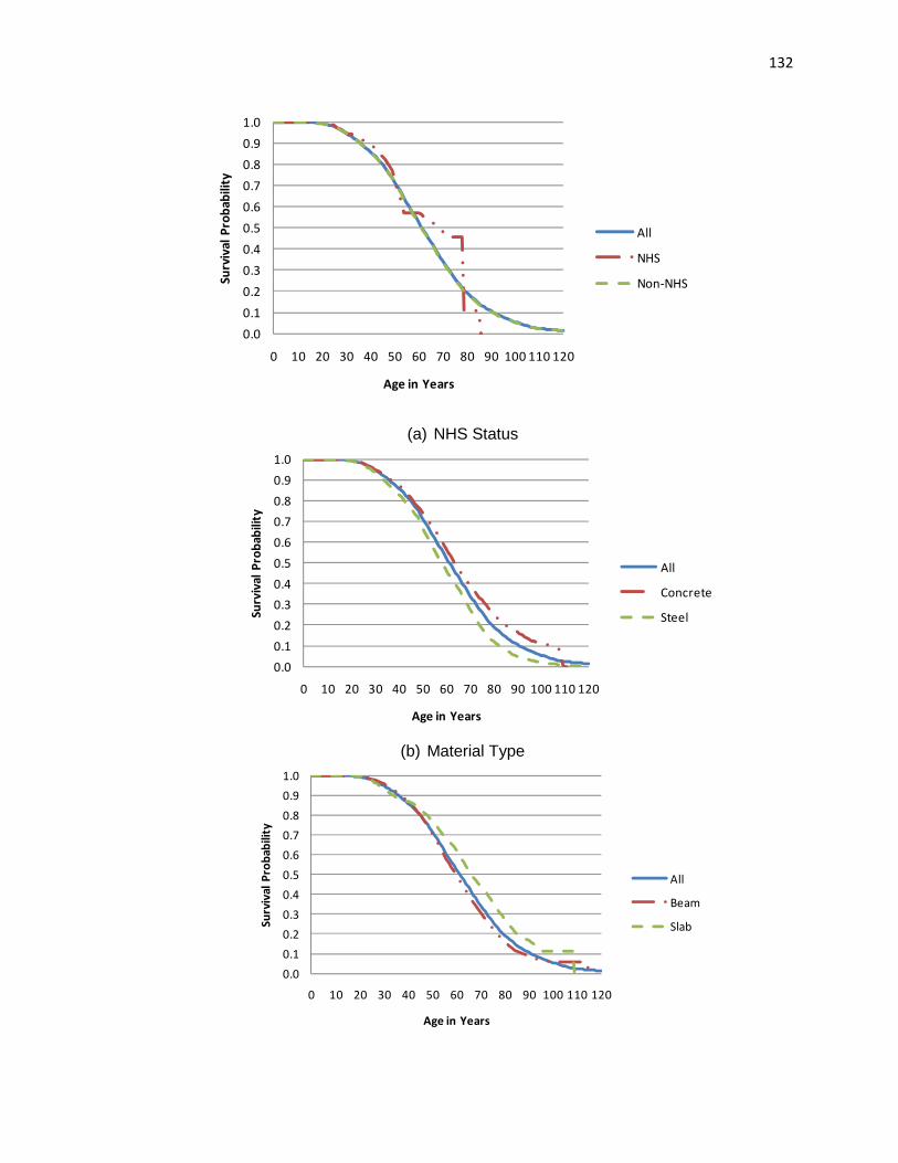
132
(a) NHS Status
(b) Material Type
0.0
0.1
0.2
0.3
0.4
0.5
0.6
0.7
0.8
0.9
1.0
0 10 20 30 40 50 60 70 80 90 100 110 120
Su
rviv
al
Pro
ba
bil
ity
Age in Years
All
NHS
Non-NHS
0.0
0.1
0.2
0.3
0.4
0.5
0.6
0.7
0.8
0.9
1.0
0 10 20 30 40 50 60 70 80 90 100 110 120
Surv
ival
Pro
bab
ility
Age in Years
All
Concrete
Steel
0.0
0.1
0.2
0.3
0.4
0.5
0.6
0.7
0.8
0.9
1.0
0 10 20 30 40 50 60 70 80 90 100 110 120
Su
rviv
al P
rob
abil
ity
Age in Years
All
Beam
Slab

133
(c) Structural Type
(d) Geographic Region
Figure 6-3: Sensitivity of Non-Covariate Indiana Bridge Superstructure Life Models
(a) NHS Status
0.0
0.1
0.2
0.3
0.4
0.5
0.6
0.7
0.8
0.9
1.0
0 10 20 30 40 50 60 70 80 90 100 110 120
Su
rviv
al P
rob
abil
ity
Age in Years
All
Urban
Rural
0.0
0.1
0.2
0.3
0.4
0.5
0.6
0.7
0.8
0.9
1.0
0 10 20 30 40 50 60 70 80 90 100 110 120
Surv
ival
Pro
bab
ility
Age in Years
All
NHS
Non-NHS
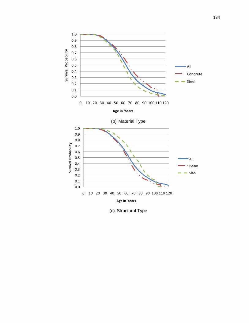
134
(b) Material Type
(c) Structural Type
0.0
0.1
0.2
0.3
0.4
0.5
0.6
0.7
0.8
0.9
1.0
0 10 20 30 40 50 60 70 80 90 100 110 120
Su
rviv
al
Pro
ba
bil
ity
Age in Years
All
Concrete
Steel
0.0
0.1
0.2
0.3
0.4
0.5
0.6
0.7
0.8
0.9
1.0
0 10 20 30 40 50 60 70 80 90 100 110 120
Su
rviv
al P
rob
abil
ity
Age in Years
All
Beam
Slab

135
(d) Geographic Region
Figure 6-4: Sensitivity of Non-Covariate Indiana Bridge Substructure Life Models
(a) NHS Status
0.0
0.1
0.2
0.3
0.4
0.5
0.6
0.7
0.8
0.9
1.0
0 10 20 30 40 50 60 70 80 90 100 110 120
Surv
ival
Pro
bab
ility
Age in Years
All
Urban
Rural
0.0
0.1
0.2
0.3
0.4
0.5
0.6
0.7
0.8
0.9
1.0
0 10 20 30 40 50 60 70 80 90 100 110 120
Su
rviv
al
Pro
ba
bil
ity
Age in Years
All
NHS
Non-NHS

136
(b) Material Type
(c) Structural Type
(d) Geographic Region
Figure 6-5: Sensitivity of Non-Covariate Indiana Bridge Channel Protection Life Models
0.0
0.1
0.2
0.3
0.4
0.5
0.6
0.7
0.8
0.9
1.0
0 10 20 30 40 50 60 70 80 90 100 110 120
Surv
ival
Pro
ba
bili
ty
Age in Years
All
Concrete
Steel
0.0
0.1
0.2
0.3
0.4
0.5
0.6
0.7
0.8
0.9
1.0
0 10 20 30 40 50 60 70 80 90 100 110 120
Surv
ival
Pro
bab
ility
Age in Years
All
Beam
Slab
0.0
0.1
0.2
0.3
0.4
0.5
0.6
0.7
0.8
0.9
1.0
0 10 20 30 40 50 60 70 80 90 100 110 120
Su
rviv
al P
rob
abil
ity
Age in Years
All
Urban
Rural

137
6.2.2 Sensitivity of Box Culvert Life Prediction
In assessing the box culvert covariate life model, the most influential factor, From the attributes shown in Table 6-3, was found to be the interstate indicator, which had a negative effect of 14 years (Figure 6-6). The most influential positive factor was found to be the use of concrete which extended life by 12 years. For the uncertainty surrounding climate, likely temperature changes will produce a range of median life estimates varying up to 1 year and precipitation up to 2 years.
Table 6-3: Range of Box Culvert Life Values for Covariate Model Sensitivity Analysis
Life Expectancy Factor Minimum Value
Assumed Value
Maximum Value
Normal Annual Temperature (°F) 50 51 53
Normal Annual Precipitation (in.) 38 43 51
Geographical classification indicator (1 if rural, 0 otherwise)
0 0 1
NHS indicator (1 if on NHS, 0 otherwise) 0 1 1
Functional class indicator (1 if on interstate, 0 otherwise)
0 1 1
Maintenance responsibility indicator (1 if state responsible, 0 otherwise)
0 1 1
Corrosive soil indicator (1 if in area where average soil is classified as highly corrosive to steel or concrete by the NRCS, 0 otherwise)
0 0 1
Acidic soil indicator (1 if in area with average soil of pH < 6.5 according to NCRS, 0 otherwise)
0 0 1
Material type indicator (1 if concrete, 0 otherwise) 0 1 1
Structure length in decimeters 140 150 160
Figure 6-6: Tornado Diagram of Covariate Box Culvert Life Model
NHS, -0.08Temperature, -0.48
Acidic pH, -3.48Corrosive Soil, -4.08
Interstate, -14.16
Length, 0.01State Maint., 1.63
Precipitation, 2.10Rural, 4.38
Concrete, 11.80
-22 -20 -18 -16 -14 -12 -10 -8 -6 -4 -2 0 2 4 6 8 10 12 14 16 18
Change in Service Life (years)
Life
Exp
ect
ancy
Fac
tor

138
Analysis of the non-covariate, Indiana box culvert life sensitivity produced the following results in Table 6-4.
• NHS box culverts had a five year longer life relative to the culvert condition rating but a seven year shorter median life as pertaining to the channel protection rating;
• Concrete structures had median life estimates ranging from 27 to 32 years in life extensions as compared to steel;
• Urban structure life was found to be longer by 6 to 11 years.
Table 6-4: Box Culvert Median Life Predictions by End-of-Life Definition and Data Segmentation
Culvert Rating ≤ 4 Channel Protection Rating ≤ 4
NHS 78 75
Non-NHS 73 82
Concrete 83 88
Steel 51 61
Urban 80 91
Rural 74 80
All IN Bridges 75 84
The non-homogenous Markov chains for the Indiana box culvert are shown in Figures 6-7 and 6-8.
(a) NHS Status
0.0
0.1
0.2
0.3
0.4
0.5
0.6
0.7
0.8
0.9
1.0
0 10 20 30 40 50 60 70 80 90 100 110 120
Su
rviv
al
Pro
ba
bil
ity
Age in Years
All
NHS
Non-NHS

139
(b) Material Type
(c) Geographic Region
Figure 6-7: Sensitivity of Non-Covariate Indiana Box Culvert Condition Life Models
0.0
0.1
0.2
0.3
0.4
0.5
0.6
0.7
0.8
0.9
1.0
0 10 20 30 40 50 60 70 80 90 100 110 120
Surv
ival
Pro
bab
ility
Age in Years
All
Concrete
Steel
0.0
0.1
0.2
0.3
0.4
0.5
0.6
0.7
0.8
0.9
1.0
0 10 20 30 40 50 60 70 80 90 100 110 120
Su
rviv
al P
rob
abili
ty
Age in Years
All
Urban
Rural

140
(a) NHS Status
(b) Material Type
(c) Geographic Region
Figure 6-8: Sensitivity of Non-Covariate Indiana Box Culvert Channel Protection Life Models
0.0
0.1
0.2
0.3
0.4
0.5
0.6
0.7
0.8
0.9
1.0
0 10 20 30 40 50 60 70 80 90 100 110 120
Surv
ival
Pro
bab
ility
Age in Years
All
NHS
Non-NHS
0.0
0.1
0.2
0.3
0.4
0.5
0.6
0.7
0.8
0.9
1.0
0 10 20 30 40 50 60 70 80 90 100 110 120
Su
rviv
al P
rob
abil
ity
Age in Years
All
Concrete
Steel
0.0
0.1
0.2
0.3
0.4
0.5
0.6
0.7
0.8
0.9
1.0
0 10 20 30 40 50 60 70 80 90 100 110 120
Su
rviv
al
Pro
bab
ilit
y
Age in Years
All
Urban
Rural

141
6.2.3 Sensitivity of Pipe Culvert Life Prediction
From the results that assess the pipe culvert model sensitivity to the characteristics shown in Table 6-5, it is clear that further enhancements to the prediction is required. Climate uncertainty (i.e., temperature, precipitation, freeze-thaw cycles) accounted for a 7-60 year wide ranges in median life predictions indicating that the parameter estimates are likely errant (Figure 6-9). As such, it is recommended to collect further data that may mitigate the heterogeneity associated with these parameters. Other factors found to significantly affect life included an extra 8 years of life for metal culverts, an extra 3 years for coating protection, and a loss of 3 years based on the soil plasticity.
Table 6-5: Range of Pipe Culvert Life Values for Covariate Model Sensitivity Analysis
Life Expectancy Factor Minimum
Value Assumed
Value Maximum
Value Normal Annual Temperature (°F) 46 47 49 Normal Annual Precipitation (in.) 40 46 54 Normal Annual Freeze-Thaw Cycles (days) 95 100 105 Material indicator (1 if plastic, 0 otherwise) 0 1 1 Material indicator (1 if metal, 0 otherwise) 0 0 1 Coating indicator (1 if coating applied, 0 otherwise) 0 1 1 Approximate area opening [height (in.) * width (in.)] 143 144 145 Plasticity Index of average soil in NRCS survey area 0 0 1
Figure 6-9: Tornado Diagram of Covariate Pipe Culvert Life Model
Opening Area, -0.02Plasticity, -3.15
F-T Cycles, -6.77Plastic, -39.28
Precip., -57.06
Coating, 3.41Metal, 8.16
Temp., 23.60
-80 -75 -70 -65 -60 -55 -50 -45 -40 -35 -30 -25 -20 -15 -10 -5 0 5 10 15 20 25 30 35 40 45 50 55
Change in Service Life (years)
Life
Exp
ect
ancy
Fac
tor
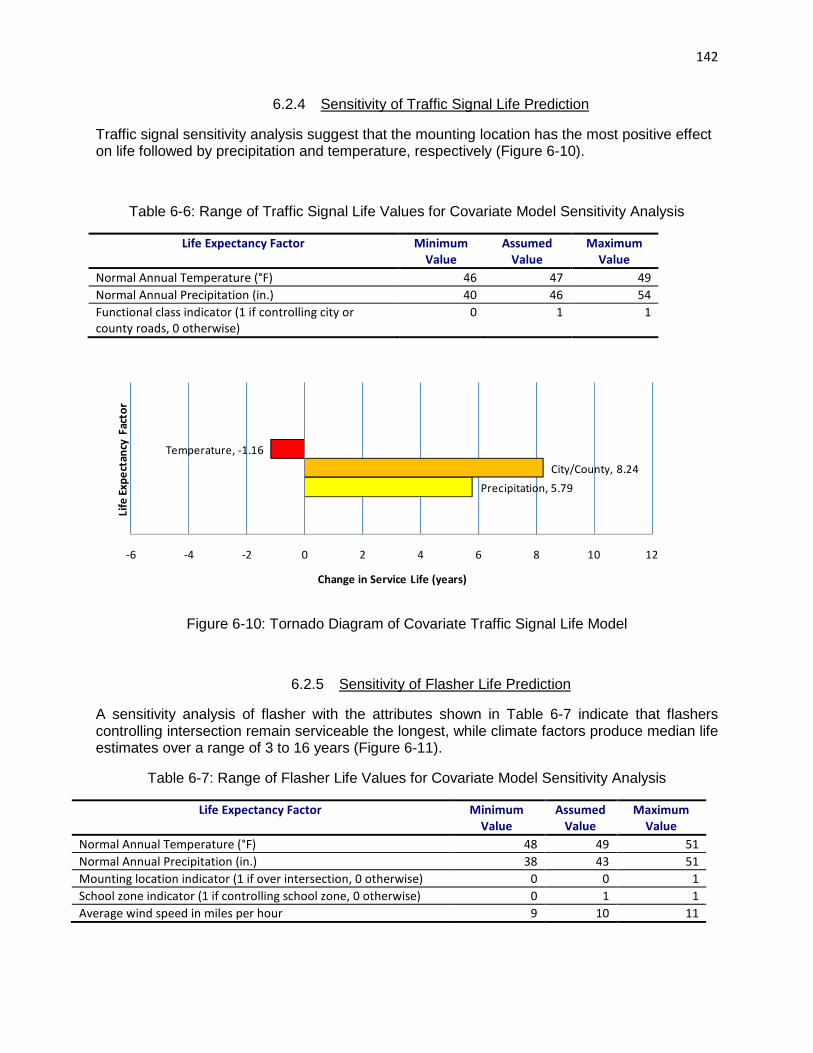
142
6.2.4 Sensitivity of Traffic Signal Life Prediction
Traffic signal sensitivity analysis suggest that the mounting location has the most positive effect on life followed by precipitation and temperature, respectively (Figure 6-10).
Table 6-6: Range of Traffic Signal Life Values for Covariate Model Sensitivity Analysis
Life Expectancy Factor Minimum
Value
Assumed
Value
Maximum
Value
Normal Annual Temperature (°F) 46 47 49
Normal Annual Precipitation (in.) 40 46 54
Functional class indicator (1 if controlling city or
county roads, 0 otherwise)
0 1 1
Figure 6-10: Tornado Diagram of Covariate Traffic Signal Life Model
6.2.5 Sensitivity of Flasher Life Prediction
A sensitivity analysis of flasher with the attributes shown in Table 6-7 indicate that flashers controlling intersection remain serviceable the longest, while climate factors produce median life estimates over a range of 3 to 16 years (Figure 6-11).
Table 6-7: Range of Flasher Life Values for Covariate Model Sensitivity Analysis
Life Expectancy Factor Minimum
Value
Assumed
Value
Maximum
Value
Normal Annual Temperature (°F) 48 49 51
Normal Annual Precipitation (in.) 38 43 51
Mounting location indicator (1 if over intersection, 0 otherwise) 0 0 1
School zone indicator (1 if controlling school zone, 0 otherwise) 0 1 1
Average wind speed in miles per hour 9 10 11
Temperature, -1.16
Precipitation, 5.79
City/County, 8.24
-6 -4 -2 0 2 4 6 8 10 12
Change in Service Life (years)
Life
Exp
ect
ancy
Fac
tor

143
Figure 6-11: Tornado Diagram of Covariate Flasher Life Model
6.2.6 Sensitivity of Roadway Lighting Life Prediction
Roadway lighting life was found to be most sensitive to the material type and mounting location (Figure 6-12). Metal poles were found to have significantly lower life estimates compared to those mounted on signs (largest positive effect).
Table 6-8: Range of Roadway Lighting Life Values for Covariate Model Sensitivity Analysis
Life Expectancy Factor Minimum
Value
Assumed
Value
Maximum
Value
Normal Annual Temperature (°F) 48 49 51
Material type indicator (1 if metal pole, 0 otherwise) 0 1 1
Mounting location indicator (1 if on sign, 0 otherwise) 0 0 1
Functional class indicator (1 if on interstate, 0 otherwise) 0 1 1
Fixture height indicator (1 if less than 30 feet, 0 otherwise) 0 0 1
Figure 6-12: Tornado Diagram of Covariate Roadway Lighting Life Model
Temperature, -3.13
School Zone, -4.22
Wind Speed, -4.98
Precipitation, -16.07
Intersection, 27.65
-35 -30 -25 -20 -15 -10 -5 0 5 10 15 20 25 30 35 40
Change in Service Life (years)
Lif
e E
xp
ect
an
cy F
act
or
Fixture Height, -5.70
Metal Pole, -34.39
Interstate, 6.83
Temperature, 10.98
Sign Mount, 36.92
-55 -50 -45 -40 -35 -30 -25 -20 -15 -10 -5 0 5 10 15 20 25 30 35 40 45 50 55
Change in Service Life (years)
Life
Exp
ect
an
cy F
acto
r

144
6.2.7 Summary of Sensitivity Analyses
In analyzing the sensitivity of the developed covariate models to various ranges of life expectancy factors, it was found that:
• Bridge life most affected by NHS status; • Box culvert life most influenced by Interstate status; • Pipe culvert life heavily dependent upon precipitation levels; • Traffic signal life influenced most by roadway functional class; • Flasher life affected primarily by mounting location; • Roadway lighting life most significantly influenced by mounting type;
Analysis of the non-covariate, constrained to the condition states of Indiana bridges and box culverts produced similar findings to the covariate sensitivity analyses. It was found that Indiana bridges were most sensitive to NHS status, while box culverts were most influenced by material type.
Furthermore, it was found that the collected data, empirically suggests that a temperature range of 3 degrees can affect bridge life by -1 year, box culvert life by -6 months, pipe culvert life by +24 years, traffic signal life by -1 year, flasher life by -3 years, and roadway lighting life by +11 years. A range of annual precipitation values varying by roughly -12% to +15% was found to influence bridge life by -1 year, box culvert life by +2 years, pipe culvert life by -57 years, traffic signal life by +6 years, and flasher life by -16 years (roadway lighting was found to not be significantly influenced by precipitation. While the extent of the influence of climate requires further study (particularly with pipe culverts), it is readily apparent that climate significantly affects infrastructure life and given the uncertainty can be analyzed further by risk assessments.
6.3 Risk Assessments of Highway Asset Replacement Decisions
For the remainder of this study, emphasis will be placed on assessing the risk of highway asset replacement decisions. First, the risk posed by uncertain climate is assessed at the project level with respect to life predictions and annual life cycle costs. Secondly, the risk of uncertain life is assessed with respect to a network-level needs assessment. This latter analysis will focus on (i) propagating the uncertain climate effects found to significantly affect the covariate model life predictions and (ii) assess the risk posed by correlated, competing ‘failure mechanisms’ via the non-covariate models. Both methods will be demonstrated using the Indiana NBI bridge database, however, similar studies can be completed for other assets contingent upon model improvement and agency preference.
6.3.1 Risk of Uncertain Future Climate
As shown in the sensitivity analyses, uncertain climate poses a risk to infrastructure life. To assess the likelihood of asset life predictions, expert opinion of probabilistic estimates of future climatic conditions were obtained for two scenarios: (i) low emissions – assuming significant action taken to reduce greenhouse gases and (ii) moderately high emissions – assuming no action taken (Figure and Figure ). Normal distributions were assumed with the standard deviation taken as the range of values experts felt were likely. In ICF International (2009),

145
emission policies had a marginal effect on short-term climate, with the moderately high emissions scenario corresponding to slightly less uncertainty and slightly higher estimates. For agencies wishing to replicate the analysis, any distribution can be used in the place of those provided.
Figure 6-13: Probabilistic Forecast of Midwest Annual Temperature Change for 2010-2040 Normals (ICF International, 2009)
Figure 6-14: Probabilistic Forecast of Midwest Annual Precipitation Change for 2010-2040 Normals (ICF International, 2009)
0.0
0.1
0.2
0.3
0.4
0.5
0.6
0.7
0 2 4 6
Pro
ba
bil
ity
Δ in Temperature (°F)
Low Emissions
~N(2.6, 0.7)
Moderately High
Emissions
~N(2.7, 0.6)
0.00
0.01
0.02
0.03
0.04
0.05
0.06
0.07
-15 -10 -5 0 5 10 15 20
Pro
bab
ility
Δ in Precipitation (in.)
Low Emissions
~N(4, 6)
Moderately High
Emissions
~N(5,7)

146
To model the dependency structure, the correlation between the random variables was evaluated over the normal annual values for every climate division in the United States over the last 30 years. With this sample, a Pearson product-moment correlation coefficient of 0.50 was found indicating the need for correlated simulation. Overall, a positive relationship was found which is consistent with the higher moisture capacity of warmer air (Figure 6-15).
Figure 6-15: Correlation Pattern of Average Annual Temperature and Precipitation over all U.S. Climate Divisions based on Current Normals
To simulate this correlation pattern, a statistical copula was fit to the data. The best fitting copula was found to be the normal copula with covariance = 0.5643 which corresponded to a -SIC of 96.96, -AIC of 100.86, and -HQIC of 99.31, using maximum likelihood estimation.
In the case of pipe culverts, additional correlation tests were conducted with respect to freeze-thaw cycles. A negative, but insignificant Pearson product moment correlation factor was found, suggesting that freeze-thaw cycles could be modeled independently. To approximate future freeze-thaw cycles, a probability distribution was fit to values obtained by randomly sampling seasonal temperature distributions for each emissions scenario from (ICF International, 2009). The resulting distribution was found to be Normal with a standard deviation of 1.66 surrounding the deterministic estimate.
Ten thousand trials were conducted for each asset class assuming the characteristics presented in the sensitivity analysis section. The change in median life values, survival curves, equivalent annual cost, and utility associated with replacing the structure for various ages were quantified.
0
20
40
60
80
100
120
140
0 10 20 30 40 50 60 70 80 90
Av
era
ge
An
nu
al
Pre
cip
ita
tio
n (
in.)
Average Annual Temperature (F)
ρ = 0.50

147
6.3.1.1 Risk Assessment of Uncertain Future Climate on Bridge Life
From the correlated simulation of temperature and precipitation and subsequent incorporation into the covariate life expectancy model, the probability of life predictions were quantified with respect to the median estimate and the overall survival curve.
In terms of the median estimate, the low emissions scenario produced a median value of 55.77 years with a 90% confidence interval of [55.06, 56.50] and the moderately high emissions scenarios produced a median value of 55.70 years with a 90% confidence interval of [55.00, 56.40] (Figure 6-16). Under the current climatic conditions (annual average temperature = 49°F and annual average precipitation = 43 in.) an estimate of 56.86 years was predicted. As such, a loss of 1.09 years and 1.16 years for the two scenarios, respectively, can be concluded the most probable. The likelihood that bridge life will be reduced, assuming the validity of the model, is 99.31% and 99.47% for the two scenarios, respectively.
Figure 6-16: Risk-based Median Bridge Life Prediction due to Climate Uncertainty
With respect to the overall survival curve, minimal changes are observable without zooming in on a percentile (Figure 6-17).
0.0
0.1
0.2
0.3
0.4
0.5
0.6
0.7
0.8
0.9
1.0
54 55 56 57
Pro
ba
bili
ty D
en
sity
Fu
nct
ion
Median Life (years)
Low Emissions
Moderately High
Emissions
Current

148
(a) Low Emissions Scenario
(b) Moderately High Emissions Scenario
Figure 6-17: Risk-based Bridge Survival Curve due to Climate Uncertainty
0.0
0.1
0.2
0.3
0.4
0.5
0.6
0.7
0.8
0.9
1.0
0 20 40 60 80 100
Pro
bab
ility
Age in years
90% Confidence
Interval
Expected
0.0
0.1
0.2
0.3
0.4
0.5
0.6
0.7
0.8
0.9
1.0
0 20 40 60 80 100
Pro
ba
bili
ty
Age in years
90% Confidence
Interval
Expected
Figure
Figure

149
6.3.1.2 Risk Assessment of Uncertain Future Climate on Box Culvert Life
With the box culvert covariate model, empirical evidence suggested that culverts in warmer climates had a significantly shorter life, while those in wet climates had significantly longer life-spans. As such, the overall effect on life with the changing climate was found to be more balanced than the effects on bridge life. In a correlated simulation of future climatic conditions with the characteristics presented previously, the effect on median life (Figure 6-18) and overall survival probabilities (Figure 6-19) were assessed.
Figure 6-18: Risk-based Median Box Culvert Life Prediction due to Climate Uncertainty
0.0
0.2
0.4
0.6
0.8
1.0
1.2
48 49 50 51 52
Pro
bab
ilit
y D
en
sity
Fu
nct
ion
Median Life (years)
Low Emissions
Moderately High
Emissions
Current

150
(a) Low Emissions Scenario
(b) Moderately High Emissions Scenario
Figure 6-19: Risk-based Box Culvert Survival Curve due to Climate Uncertainty
0.0
0.1
0.2
0.3
0.4
0.5
0.6
0.7
0.8
0.9
1.0
0 20 40 60 80 100
Pro
bab
ility
Age in years
90% Confidence
Interval
Expected
0.0
0.1
0.2
0.3
0.4
0.5
0.6
0.7
0.8
0.9
1.0
0 20 40 60 80 100
Pro
bab
ility
Age in years
90% Confidence
Interval
Expected
Figure
Figure

151
As a result of the analysis, it was found that the median estimate in the low emissions scenario produced a value of 50.03 years with a 90% confidence interval of [49.42, 50.64] and the moderately high emissions scenarios yielded a value of 50.09 years with a 90% confidence interval of [49.39, 50.81] (Figure 6-18). Under the current climatic conditions (annual average temperature = 49°F and annual average precipitation = 43 in.) an estimate of 50.18 years was predicted. As such, a loss of 1.80 months and 1.08 months for the two scenarios, respectively, can be concluded the most probable. The likelihood that box culvert life will be reduced, assuming the validity of the model, is 65.57% and 58.71% for the two scenarios, respectively.
6.3.1.3 Risk Assessment of Uncertain Future Climate on Pipe Culvert Life
In the analysis of pipe culverts, it was found that temperature had a positive impact on asset life while precipitation values and freeze-thaw cycles had a negative effect. With wide variability in precipitation and greater influence of temperature on asset life than freeze-thaw cycles, it was found that the uncertain climate will likely lead to longer culvert service life. Median life estimates were found to vary from 35.58 years (90% C.I. = [16.11, 78.45]) in the low emissions scenario, 34.48 years (90% C.I. = [14.25, 84.14]) in the moderately high emissions scenario, and 18.26 years under the current climatic conditions (annual temperature = 47°F, annual precipitation = 46 in. (Figure 6-20). In the low emissions scenario a longer life of 17.32 years was found, as compared to a 16.22 year life extension in the moderately high emissions scenario. From the risk assessment, there was found to be an 8.30% chance of a reduced median life in the low emissions scenario, and 11.88% reduced life in the moderately high emissions scenario.
Figure 6-20: Risk-based Median Pipe Culvert Life Prediction due to Climate Uncertainty
0.000
0.005
0.010
0.015
0.020
0.025
0.030
0 20 40 60 80 100
Pro
bab
ilit
y D
en
sity
Fu
nct
ion
Median Life (years)
Low Emissions
Moderately High
Emissions
Current

152
The wide variability in life predictions can further be seen in Figure 6-21, indicating that an improved model is needed.
(a) Low Emissions Scenario
(b) Moderately High Emissions Scenario
Figure 6-21: Risk-based Pipe Culvert Survival Curve due to Climate Uncertainty
0.0
0.1
0.2
0.3
0.4
0.5
0.6
0.7
0.8
0.9
1.0
0 20 40 60 80 100
Pro
ba
bili
ty
Age in years
90% Confidence
Interval
Expected
0.0
0.1
0.2
0.3
0.4
0.5
0.6
0.7
0.8
0.9
1.0
0 20 40 60 80 100
Pro
bab
ility
Age in Years
90% Confidence
Interval
Expected
Figure
Figure

153
6.3.1.4 Risk Assessment of Uncertain Future Climate on Traffic Signal Life
A probabilistic risk assessment of traffic signal life due to uncertain climate produced the range of median life estimates in Figure 6-22. With both temperature and precipitation found to have positive influences on life, it was found that the future median life estimate will be extended with over 99.99% confidence with a median life extension of 4.98 years for the low emissions scenario and 5.14 years for the moderately high emissions scenario. The current median life prediction (annual temperature = 47°F, annual preci pitation = 46 in.) was found to be 20.95 years, 25.93 years (90% C.I. = [24.14, 27.86]) for the low emissions scenario, and 26.09 years (90% C.I. = [24.03, 28.30]) for the moderately high emissions scenario.
Figure 6-22: Risk-based Median Traffic Signal Life Prediction due to Climate Uncertainty
The survival curves were found to be most uncertain between ages 26 and 31 years (Figure 6-23).
0.00
0.05
0.10
0.15
0.20
0.25
0.30
0.35
0.40
20 25 30 35
Pro
bab
ility
De
nsi
ty F
un
ctio
n
Median Life (years)
Low Emissions
Moderately High
Emissions
Current

154
(a) Low Emissions Scenario
(b) Moderately High Emissions Scenario
Figure 0-8: Risk-based Traffic Signal Survival Curve due to Climate Uncertainty
0.0
0.1
0.2
0.3
0.4
0.5
0.6
0.7
0.8
0.9
1.0
0 20 40 60 80 100
Pro
bab
ility
Age in years
90% Confidence
Interval
Expected
0.0
0.1
0.2
0.3
0.4
0.5
0.6
0.7
0.8
0.9
1.0
0 20 40 60 80 100
Pro
ba
bili
ty
Age in years
90% Confidence
Interval
Expected
Figure
Figure

155
6.3.1.5 Risk Assessment of Uncertain Future Climate on Flasher Life
Flasher life was found to be negatively influenced by both temperature and precipitation. However, given the uncertainty in future precipitation there was found to be a 9.94% chance of a longer median life under the low emissions scenario and 9.68% chance of longer life under the moderately high emissions scenario. The median predictions, for the characteristics defined in the sensitivity analysis, were found to be 21.80 years with current climatic conditions (annual temperature = 49°F, annual precipitation = 43 in.), 17.30 years (90% C.I. = [12.99, 23.24]) with the low emissions scenario, and 16.77 years with the moderately high emissions scenario (90% C.I. = [12.35, 23.31]) (Figure 6-24). These findings equate to an average life shortened by 4.50 and 5.03 years respectively.
Figure 6-24. Risk-based Median Flasher Life Prediction due to Climate
In assessing the survival curves, greater uncertainty occurs as the asset ages (Figure ).
0.00
0.02
0.04
0.06
0.08
0.10
0.12
0.14
5 10 15 20 25 30
Pro
bab
ility
De
nsi
ty F
un
ctio
n
Median Life (years)
Low Emissions
Moderately High
Emissions
Current

156
(a) Low Emissions Scenario
(b) Moderately High Emissions Scenario
Figure 6-25: Risk-based Flasher Survival Curve due to Climate Uncertainty
0.0
0.1
0.2
0.3
0.4
0.5
0.6
0.7
0.8
0.9
1.0
0 20 40 60 80 100
Pro
bab
ilit
y
Age in years
90% Confidence
Interval
Expected
0.0
0.1
0.2
0.3
0.4
0.5
0.6
0.7
0.8
0.9
1.0
0 20 40 60 80 100
Pro
ba
bili
ty
Age in years
90% Confidence
Interval
Expected
Figure
Figure

157
6.3.1.6 Risk Assessment of Uncertain Future Climate on Roadway Lighting Life
In the risk assessment of roadway lighting life, based on the characteristics described in the sensitivity analysis, longer life-spans were found. This corresponds to the finding of assets with significantly longer lives in warmer climates. With precipitation not found to have a significant effect on life, a non-correlated Monte Carlo simulation was conducted. From the analysis, it was found that the median life prediction varied from 30.19 years (90% C.I. = [24.97, 36.6]) to 30.71 years (90% C.I. = [25.86, 36.43]) in the two emissions scenarios (Figure 6-26). These estimates were found to be 10.89 and 11.41 years longer than the 19.3 years of median life under the current climate scenario (annual temperature = 49°F).
Figure 6-26: Risk-based Median Roadway Lighting Life Prediction due to Climate
As with the flashers, upon analyzing the survival curves, the uncertainty was found to propagate with age (Figure 6-27).
0.00
0.02
0.04
0.06
0.08
0.10
0.12
0.14
15 20 25 30 35 40 45
Pro
bab
ilit
y D
en
sity
Fu
nct
ion
Age in years
Low Emissions
Moderately High
Emissions
Current

158
(a) Low Emissions Scenario
(b) Moderately High Emissions Scenario
Figure 6-27: Risk-based Roadway Lighting Survival Curve due to Climate Uncertainty
0.0
0.1
0.2
0.3
0.4
0.5
0.6
0.7
0.8
0.9
1.0
0 20 40 60 80 100
Pro
ba
bil
ity
Age in years
90% Confidence
Interval
Expected
0.0
0.1
0.2
0.3
0.4
0.5
0.6
0.7
0.8
0.9
1.0
0 20 40 60 80 100
Pro
ba
bil
ity
Age in years
90% Confidence
Interval
Expected
Figure
Figure

159
6.3.2 Risk-based Needs Assessment
Given the uncertainty of asset life, the fiscal and physical long-term needs of an agency are inherently uncertain. To demonstrate how to quantify this uncertainty, probabilistic risk assessments of various scenarios are examined and compared using the 2009 Indiana bridge database. Three general variations of risk-based needs assessments were analyzed over a 15 year planning horizon:
1) Hybrid age/condition-based, probabilistic assessment of replacement needs given recently observed climatic conditions and uncertain future climatic conditions;
2) Condition-based, probabilistic assessment of replacement needs for varying and maintenance strategies;
3) Deterministic assessments of replacement needs for varying estimates of life and modeling techniques.
The first scenario utilizes the developed covariate model to assess the risk of uncertain climate on budget needs. Scenario 2 compares the uncertain budget needs based on varying definitions of what constitutes a serviceable bridge (e.g., Substructure Rating ≥ 4, Substructure and Superstructure rating ≥ 4, Substructure, Superstructure, and Channel rating ≥ 4 and Deck Geometry rating ≥ 3) and what maintenance strategies are pursued during the remainder of the life estimate (e.g., rehab superstructure at rating = 5 and substructure at rating = 5, do nothing). Scenario 3 can be compared to each of the other scenarios to assess the risk of not developing a probabilistic life expectancy model.
The cost of replacement for each bridge was assumed to be the sum of the Cobb-Douglas functions in Table 6-9, which were applied over the entire Indiana 2009 bridge stock (Figure 6-28).
Table 6-9 Assumed Bridge Replacement Costs (Sinha et al., 2009)
Cost Component Bridge Type ��� � 2 �� 2 �
Superstructure
Replacement
Reinforced Concrete Slab a = 0.0488; b =0.899; c = 1
Concrete Beam/Girder a = 0.0513; b = 0.979; c = 0.828
Steel Beam/Girder a = 0.123; b = 1; c = 0.519
Other a = 0.0885; b = 0.906; c = 0.747
Substructure
Replacement
Reinforced Concrete Slab a = 0.120; b = 0.727; c = 0.602
Other a = 0.028; b = 0.936; c = 0.983
Approach (L=500) a = 0.769; b = 0.823; c = 0
Other a = 0.721; b = 0.696; c = 0.932

160
Figure 6-28: Histogram of Bridge Age for Indiana Stock as of 2009
For each scenario, the total budget needs in present worth (assuming an interest rate of 4%) over a 15 year planning horizon were analyzed. Likewise, the number and percentage of assets expected to need one or more replacements within the planning horizon were noted.
6.3.2.1 Hybrid Age/Condition-based, Probabilistic Needs Assessment
In Scenario 1, three risk analyses were conducted on the covariate bridge life model that predicted the time until the NBI sufficiency rating dropped to or below 50%, in order to assess the present worth of replacement needs from 2009-2023:
A) Simulation of bridge life using current climate inputs; B) Simulation of bridge life using uncertain future climate inputs under the low emissions
scenario; C) Simulation of bridge life using uncertain future climate inputs under the moderately high
emissions scenario.
In Scenario 1A, a Weibull distributed random variable was sampled from the conditional survival probability curve unless the sufficiency rating was already below 50%, indicating zero remaining life. For active assets not inspected in 2009, the time between the year of inspection and 2009 was subtracted from the random life variable, with a minimum possible remaining life value bounded by zero. Likewise, a planning gap can be subtracted from the random value based on agency preferences (e.g., probabilistic delay in replacement applied in (van Noortwijk & Klatter, 2004) using renewal theory). For structures that had a remaining service life within the planning horizon, a second life prediction was simulated using the unconditional survival model. Likewise, in the off chance of failing more than twice within the planning horizon, five life predictions were contingently estimated. However, in the simulations only 0.2% of active structures required more than one replacement. If the remaining life extended beyond the planning horizon, then no costs were added to the needs assessment, else the present worth of the replacement cost was added to the fiscal needs. Each structure was assumed to have an
0
0.1
0.2
0.3
0.4
0.5
0.6
0.7
0.8
0.9
1
0
50
100
150
200
250
300
0 10 20 30 40 50 60 70 80 90 100110120130140150
Cu
mu
lati
ve F
req
ue
ncy
Nu
mb
er
of
Ind
ian
a B
rid
ges
Age in Years

161
independent service life estimate, however future studies may add to the literature by assessing potential spatial correlation effects. This simulation was conducted over 10,000 trials.
In following this approach for the current climate, it was found that on average $1.749 billion was needed for 3,620 bridges (22.5% of stock) in 2009 to meet the replacement needs under this life definition. Of the trials, it was found that for 90% confidence, a minimum of $1.800 billion was needed and that 3,554 (22.0%) to 3,686 (22.9%) structures would need replacement. As such, to improve confidence from 50% to 90%, a contingency fund of $51 million should have been set aside in 2009. For 99.99% confidence a contingency of $123 million is needed.
In Scenarios 1B and 1C, the analysis was repeated with the addition of random temperature and precipitation values, with dependencies drawn from the copula described in a previous section.
The probabilistic needs assessment was then conducted over 10,000 trials with the correlated simulation of temperature and precipitation inputted into the life expectancy model for each emissions scenario. The random simulation of the uncertain life was then conducted as in Scenario 1A. The resulting probabilistic needs assessment indicated an average value of $1.798 billion and 3,712 (23.1%) ‘failed’ structures under the low emissions scenario and $1.801 billion and 3,720 (23.1%) ‘failed’ structures under the moderately high emissions scenario. For 90% confidence a minimum value of $1.855 billion and 3,784 (23.5%) ‘failed’ structures was found to be needed for the low emissions scenario and $1.859 billion and 3,790 (23.5%) ‘failed’ structures for the moderately higher emissions scenario. This suggests that to increase confidence to 90%, a contingency of $57 million is needed under the low emission scenario and $58 million is needed under the moderately high emissions scenario. For 99.99% confidence, $176 million and $178 million are needed for the low and moderately high emission scenarios, respectively.
In comparing the estimates, it was found that on average, the uncertain climate will result in an additional $49 million and $52 million over the next 15 years for replacement projects given the low and moderately high emission scenarios, respectively (Figure 6-29).
Figure 6-29: Uncertainty in Present Worth of 15 Year Replacement Needs by Climate Conditions
0.0E+00
2.0E-09
4.0E-09
6.0E-09
8.0E-09
1.0E-08
1.2E-08
$1.60 $1.70 $1.80 $1.90 $2.00
Pro
bab
ility
De
nsi
ty F
un
ctio
n
Present Worth of 15 year Bridge Replacement Needs ($ Billions)
Current
Low Emissions
Moderately High
Emissions

162
In terms of the number of structures needing replacement it was found that on average an additional 92 to 100 replacements (0.6% of the stock) were required (Figure 6-30).
.
Figure 6-30: Uncertainty in Number of Bridges Needing Replacement within Planning Horizon by Climate Conditions
The minimum amount needed with respect to varying confidence levels describe the stochastic dominance of the moderately high emission scenario to the low emission scenario and the current climate scenario respectively (Figure 6-31).
Figure 6-31: Minimum Present Worth of Bridge Replacement Needs within Planning Horizon by Confidence Level and Climate Conditions
0
0.001
0.002
0.003
0.004
0.005
0.006
0.007
0.008
0.009
3,400 3,600 3,800 4,000
Pro
bab
ilit
y D
en
sity
Fu
nct
ion
No.of Bridges Needing Replacement in 15 Year Planning Horizon
Current
Low Emissions
Moderately High
Emissions
0%
10%
20%
30%
40%
50%
60%
70%
80%
90%
100%
$1.65 $1.75 $1.85 $1.95
Co
nfi
de
nce
Le
vel
Minimum PW of 15 Year Bridge Replacement Needs ($Billions)
Current
Low Emissions
Moderately High
Emissions

163
6.3.2.2 Condition-based, Probabilistic Needs Assessment
While age-based models are more commonly used for fiscal analysis, a condition-based needs prediction was also assessed for the remaining life of the current asset stock in order to better accommodate varying maintenance activity decisions. Two risk assessments were completed with varying definitions of life and varying maintenance strategies:
A) Simulation of bridge life, with respect to superstructure, and substructure condition, assuming no remaining major maintenance activities other than deck replacements;
B) Simulation of bridge life, with respect to superstructure and substructure condition, assuming superstructure and substructure rehabilitation activities (assume life extensions beyond remaining time within planning horizon) at the time of deck replacement;
This method is advantageous when dealing with assets that have unique life profiles, agencies wish to assess different life thresholds, evaluate different condition-based strategies, and when an agency is interested in the dominating ‘failure mechanism’ (e.g., if believe substructure will dominate then may mitigate by applying a substructure rehabilitation activity). The main disadvantages of this approach are the inability to directly adjust for climate covariates, unless sufficient data is available to model transition probabilities as a function of such independent factors. However, the acceleration parameters found for the covariate models can be used to scale the condition-based survival curves.
To predict the remaining life of models, a Beta distribution was fit to the remaining life according to the Markov chain with an initial state vector corresponding to the current age and respective condition state. To simulate multiple, correlated life estimates based on each ‘failure mechanism’, a copula was fit based on the current median life predictions of the current Indiana NBI stock.
The correlation matrix (Table 6-10) between remaining deck, superstructure, and substructure life showed a strong correlation between the remaining life of bridge elements.
Table 6-10: Correlation Matrix of Remaining Indiana Deck, Superstructure, & Substructure Life
Deck RSL Superstructure RSL Substructure RSL
Deck RSL 1 0.74 0.70
Superstructure RSL 0.74 1 0.81
Substructure RSL 0.70 0.81 1
To probabilistically model this dependence, a multivariate copula was fit to represent the correlation between deck life, superstructure life, and substructure life. The best fitting copula was found to be of the Clayton form (α=3.758) with -SIC = 16,272.87, -AIC = 16,280.67, and -HQIC = 16,278.11.
By randomly sampling the dependency from the copula and the remaining service life for decks, superstructures, and substructures from the Beta distributions for every asset in the active Indiana bridge stock, the total present worth of replacement needs were quantified.
In Scenario 2A, it was found that in 2009, the median present worth of fiscal replacement needs was $1.962 billion with 3,884 bridges (24.12% of stock) requiring total replacement

164
(Figures 6-32 and 6-33) and $850 million (Figure 6-34) over 5,466 decks for deck replacements (Figure 6-35 - same for scenario 2B except quantifies deck replacement and rehabilitation activities). This corresponds to an overall fiscal need, excluding minor maintenance/preservation activities, of $2.811 billion (Figure 6-36). For 90% confidence, it was found that a minimum of $2.865 billion was needed (Figure 6-37) over 3,821 (23.73% of stock) to 3,944 (24.50% of stock) structures would need total replacement and 5,386 (33.45% of stock) to 5,545 (34.44% of stock) would need a deck replacement. As such, to improve confidence from 50% to 90%, an overall contingency fund of $54 million should have been set aside in 2009. For 99.99% confidence a contingency of $175 million is needed.
Figure 6-32: Uncertainty in Present Worth of 15 Year Total Bridge Replacement Needs Assuming Replacement Only Strategy
Figure 6-33: Uncertainty in Number of Bridges Needing Total Replacement Assuming Replacement Only Strategy
0.0E+00
2.0E-09
4.0E-09
6.0E-09
8.0E-09
1.0E-08
1.2E-08
1.4E-08
$1.80 $1.85 $1.90 $1.95 $2.00 $2.05 $2.10 $2.15
Pro
bab
ilit
y D
en
sity
Fu
nct
ion
Present Worth of 15 year Total Replacement Needs ($ Billions)
0.000
0.001
0.002
0.003
0.004
0.005
0.006
0.007
0.008
0.009
0.010
0.011
3,725 3,775 3,825 3,875 3,925 3,975 4,025
Pro
ba
bil
ity
De
nsi
ty F
un
ctio
n
No. of Bridges Needing Total Repl. in 15 year Planning Horizon

165
Figure 6-34: Uncertainty in Present Worth of 15 Year Bridge Deck Replacement Needs Assuming Replacement Only Strategy
Figure 6-35: Uncertainty in Number of Bridge Deck Activities
0.0E+00
4.0E-09
8.0E-09
1.2E-08
1.6E-08
2.0E-08
2.4E-08
2.8E-08
$775 $800 $825 $850 $875 $900 $925
Pro
ba
bil
ity
De
nsi
ty F
un
ctio
n
Present Worth of 15 year Deck Replacement Needs ($ Millions)
0.000
0.001
0.002
0.003
0.004
0.005
0.006
0.007
0.008
0.009
5,300 5,350 5,400 5,450 5,500 5,550 5,600 5,650
Pro
bab
ility
De
nsi
ty F
un
ctio
n
No. of Bridges Needing Deck Activity in 15 year Planning Horizon

166
Figure 6-36: Uncertainty in Present Worth of 15 Year Overall Bridge Replacement Needs Assuming Replacement Only Strategy
Figure 6-37: Minimum Present Worth of Overall Replacement Needs within Planning Horizon by Confidence Level for Replacement Only Strategy
In Scenario 2B, with the same copula dependency and Beta distributions, a correlated Monte Carlo simulation was performed. If the remaining superstructure or substructure service life dominated the remaining deck service life and occurs within the next 15 years, then the full replacement cost was added to the needs assessment. If the remaining deck life dominates and occurs within the next 15 years, then the sum of costs in Table 6-11 were added to the needs assessment:
0.0E+00
2.0E-09
4.0E-09
6.0E-09
8.0E-09
1.0E-08
1.2E-08
$2.65 $2.70 $2.75 $2.80 $2.85 $2.90 $2.95 $3.00
Pro
bab
ility
De
nsi
ty F
un
ctio
n
Present Worth of 15 year Overall Replacement Needs ($ Billions)
0%
10%
20%
30%
40%
50%
60%
70%
80%
90%
100%
$2.70 $2.75 $2.80 $2.85 $2.90 $2.95 $3.00
Co
nfi
de
nce
Le
vel
Minimum PW of 15 year Overall Replacement Needs ($ Billions)

167
Table 6-11: Assumed Deck Replacement, Superstructure Rehabilitation, and Substructure Rehabilitation Costs (Sinha et al., 2009)
Cost Component ��� � 2 �� 2 � Deck Replacement a = 0.035; b =1; c = 1 Superstructure Rehabilitation a = 0.0035; b = 1; c = 1 Substructure Rehabilitation a = 0.010; b = 1; c = 1
The life extension of the rehabilitation activities were assumed to extend beyond the remaining time within the planning horizon. This is considered reasonable with life extension estimates of 25 years for superstructure life and 20 years for substructure life (Sinha et al., 2009). Probabilistic estimates of the treatment life can be incorporated in future research.
Following this approach, it was found that on average $1.181 billion would be needed for bridge replacement (Figure 6-38) and $1.143 billion for deck replacement, superstructure rehabilitation, and substructure rehabilitation (Figure 6-39). In applying this maintenance strategy, 2,149 bridges (90% C.I. = [2,115, 2,185]) required total replacement (Figure 6-40). Overall, this corresponds to $2.324 billion in present worth fiscal needs (Figure 6-41). For 90% confidence, it was found that at least $2.363 billion was needed for overall replacement needs. These findings would suggest that contingency funds, relative to the median, for 90% confidence should be $38 million and $122 million for 99.99% confidence.
Figure 6-38: Uncertainty in Present Worth of 15 Year Total Bridge Replacement Needs Assuming Rehabilitation Strategy
0.0E+00
2.0E-09
4.0E-09
6.0E-09
8.0E-09
1.0E-08
1.2E-08
1.4E-08
1.6E-08
1.8E-08
$1.05 $1.10 $1.15 $1.20 $1.25 $1.30
Pro
ba
bili
ty D
en
sity
Fu
nct
ion
Present Worth of 15 year Total Replacement Needs ($ Billions)

168
Figure 6-39: Uncertainty in Present Worth of 15 Year Bridge Deck Replacement Needs Assuming Rehabilitation Strategy
Figure 6-40: Uncertainty in Number of Bridges Needing Total Replacement Assuming Rehabilitation Strategy
0.0E+00
2.0E-09
4.0E-09
6.0E-09
8.0E-09
1.0E-08
1.2E-08
1.4E-08
1.6E-08
1.8E-08
2.0E-08
$1.05 $1.10 $1.15 $1.20 $1.25
Pro
bab
ilit
y D
en
sity
Fu
nct
ion
Present Worth of 15 year Deck Repl. & Rehab. Needs ($ Billions)
0.000
0.002
0.004
0.006
0.008
0.010
0.012
0.014
0.016
0.018
0.020
2,050 2,100 2,150 2,200 2,250
Pro
bab
ility
De
nsi
ty F
un
ctio
n
No. of Bridges Needing Total Repl. in 15 year Planning Horizon

169
Figure 6-41: Uncertainty in Present Worth of 15 Year Overall Bridge Replacement Needs Assuming Rehabilitation Strategy
Figure 0-9: Minimum Present Worth of Overall Replacement Needs within Planning Horizon by Confidence Level for Rehabilitation Strategy
In comparing the needs of the replacement only option and the strategy of doing rehabilitation work at the time of deck replacements, an overall, average benefit of $487 million was found to be saved in applying the rehabilitation strategy. This corresponds to a $781 reduction in total bridge replacement costs while deck replacement costs went up $293 million with the addition of rehabilitation actions.
0.0E+00
2.0E-09
4.0E-09
6.0E-09
8.0E-09
1.0E-08
1.2E-08
1.4E-08
1.6E-08
$2.20 $2.25 $2.30 $2.35 $2.40 $2.45 $2.50
Pro
ba
bil
ity
De
nsi
ty F
un
ctio
n
Present Worth of 15 year Overall Replacement Needs ($ Billions)
0%
10%
20%
30%
40%
50%
60%
70%
80%
90%
100%
$2.25 $2.30 $2.35 $2.40 $2.45
Co
nfi
de
nce
Le
vel
Minimum PW of 15 year Overall Replacement Needs ($ Billions)

170
With respect to the age-based approach, the replacement costs of the replacement only strategy were 12% greater and the replacement costs of the selected strategy were 48% lower over the next 15 years. This suggests, that sufficiency ratings are a less restrictive measure than the applied condition-based definition of life and that the maintenance strategy is an improvement over those that led to the sufficiency-based survival time.
6.3.2.3 Deterministic Needs Assessments
Oftentimes, expert opinion is used for fiscal needs assessments with agencies assuming that blanket replacements will be applied at a certain point in time or that all structures will survive to a point estimate of life. As such, the risk of assuming any point estimate of life can be assessed in comparison to probabilistic estimates of needs. To demonstrate this approach, a deterministic needs assessment was conducted under six scenarios:
A) Single point estimate of asset life B) Deterministic application of Scenario 1A; C) Deterministic application of Scenario 1B; D) Deterministic application of Scenario 1C; E) Deterministic application of Scenario 2A; F) Deterministic application of Scenario 2B.
In Scenario 3A, a needs assessment was conducted assuming various point estimates of life (Figures 6-43 and 6-44). For instance, if the life is assumed to be 60 years then $760 million over 2,303 bridge replacements (14.3% of stock) is needed. However, as demonstrated in the previous sections, this estimate significantly underestimates fiscal needs. As such the use of a 60 year point estimate would put an agency at risk, on average, for an underestimation of $421 million to $1.202 billion in fiscal needs and underestimating total replacements in physical needs by 1,581 to overestimating needs by 154 structures (Table 6-12).
Table 6-12: Risk of Underestimating Long-term Fiscal Needs by Scenario if Assume 60 Year Life for All Structures
Scenario Fiscal Under(Over) -estimation Relative to Median Value
Physical Under(Over) -estimation Relative to Median Value
1A $989 million 1,317 structures 1B $1.038 billion 1,409 structures 1C $1.041 billion 1,417 structures 2A $1.202 billion 1,581 structures 2B $421 million (154) structures

171
Figure 6-43: Deterministic Needs Assessment of 15 year Indiana Bridge Replacements by Life Expectancy Estimate
Figure 6-44: Number of Indiana Bridges Requiring Replacement within a 15 Year Planning Horizon
For the remaining sub-scenarios, the deterministic application of the developed models was assessed. This approach, considered to be the most commonly applied, along with historical projections based on previous expenditures, (Sinha et al., 2005), assumes that all structures will survive to their median life estimate. Intuitively, this technique makes sense on a project-level, however the odds of an entire network converging to their respective median value is highly improbable. In reality, the full survival curve should be considered. Consider a set of 10 bridge assets that are predicted to have a survival probability of 60% over the next 15 years
$0
$1
$2
$3
$4
$5
$6
$7
$8
$9
$10
20 30 40 50 60 70 80 90 100 110 120
Pre
sen
t W
ort
h o
f 1
5 y
ea
r B
rid
ge
Re
pla
cem
en
t N
ee
ds
($B
illio
ns)
Point Estimate of Life Expectancy in Years
0
2,000
4,000
6,000
8,000
10,000
12,000
14,000
16,000
20 30 40 50 60 70 80 90 100 110 120
Nu
mb
er
of
Bri
dg
e R
ep
lace
me
nts
Ne
ed
ed
in 1
5 Y
ear
Ho
rizo
n
Point Estimate of Life Expectancy in Years
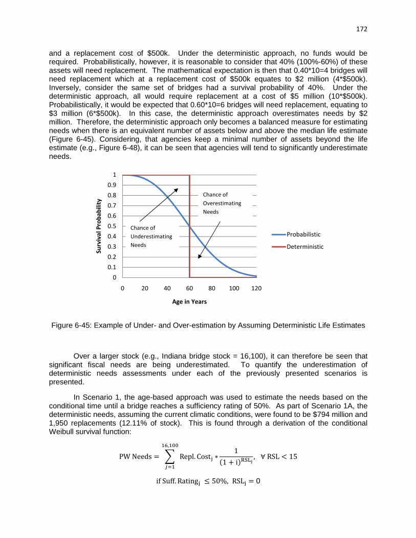
172
and a replacement cost of $500k. Under the deterministic approach, no funds would be required. Probabilistically, however, it is reasonable to consider that 40% (100%-60%) of these assets will need replacement. The mathematical expectation is then that 0.40*10=4 bridges will need replacement which at a replacement cost of $500k equates to $2 million (4*$500k). Inversely, consider the same set of bridges had a survival probability of 40%. Under the deterministic approach, all would require replacement at a cost of $5 million (10*$500k). Probabilistically, it would be expected that 0.60*10=6 bridges will need replacement, equating to $3 million (6*$500k). In this case, the deterministic approach overestimates needs by $2 million. Therefore, the deterministic approach only becomes a balanced measure for estimating needs when there is an equivalent number of assets below and above the median life estimate (Figure 6-45). Considering, that agencies keep a minimal number of assets beyond the life estimate (e.g., Figure 6-48), it can be seen that agencies will tend to significantly underestimate needs.
Figure 6-45: Example of Under- and Over-estimation by Assuming Deterministic Life Estimates
Over a larger stock (e.g., Indiana bridge stock = 16,100), it can therefore be seen that significant fiscal needs are being underestimated. To quantify the underestimation of deterministic needs assessments under each of the previously presented scenarios is presented.
In Scenario 1, the age-based approach was used to estimate the needs based on the conditional time until a bridge reaches a sufficiency rating of 50%. As part of Scenario 1A, the deterministic needs, assuming the current climatic conditions, were found to be $794 million and 1,950 replacements (12.11% of stock). This is found through a derivation of the conditional Weibull survival function:
PW Needs � \ Repl. Cost� 2`Æ,`QQ�_`
1�1 � i����� , ∀ RSL À 15
if Suff. Rating� Á 50%, RSL� � 0
0
0.1
0.2
0.3
0.4
0.5
0.6
0.7
0.8
0.9
1
0 20 40 60 80 100 120
Su
rviv
al
Pro
ba
bil
ity
Age in Years
Probabilistic
Deterministic
Chance of
Underestimating
Needs
Chance of
Overestimating
Needs

173
else, RSL� � b� ���] d0.5 2 ��A�Ë �j� B§f§ � [���
If conditional survival was not considered, it was found the needs would have been estimated at $1.154 billion and 2,803 replacements (17.41% of stock); which demonstrates the importance of updating survival probabilities. The deterministic, conditional survival estimate would put an agency at risk for underestimating fiscal needs by $955 million and physical needs by 1,670 replacements.
For Scenarios 1B and 1C the same calculation was performed using the estimated future climatic conditions for the two emission scenarios, resulting in new βj values. Under Scenario 1B, with an expected temperature change of 2.6 and precipitation change of +4%, the deterministic fiscal needs were evaluated at $803 million and 1,999 replacements (12.42% of stock) for the low emissions scenario. Under Scenario 1C, with an expected temperature change of 2.7 and precipitation change of +5%, the same deterministic estimates of fiscal and physical needs were found for the moderately high emissions scenario due to insignificant changes in expected climatic conditions between the emissions scenarios.
Finally, a deterministic application of remaining service life using the condition-based approaches under varying maintenance strategies were assessed. In the case of no rehabilitation activities, a deterministic fiscal and physical estimate of $1.566 billion and 3,526 of the active bridges requiring total replacement (21.90% of stock with 76.34% ‘failing’ due to the superstructure end-of-life measure) were obtained, respectively. This corresponds to an additional $775 million and 5,644 bridge decks (35.06% of stock) requiring replacement throughout the total structure life, resulting in an overall fiscal needs of $2.342 billion. As a result, an agency would be at risk for underestimating fiscal needs by $469 million and physical needs by 358 active bridge requiring replacement, along with an overestimation of 178 active decks requiring replacement.
When the designated maintenance strategy was applied, fiscal needs were found to be $450 million for bridge replacement and $1.267 billion for rehabilitation and deck replacement activities; physical needs were found to be 985 replacements (6.12% of stock) and 6,615 maintenance activities (41.09% of stock). Overall fiscal needs of this approach result in an estimate of $1.717 billion, a savings of $625 million compared to the replacement only strategy. The resulting risk of deterministically applying this approach was found to be underestimating fiscal needs by $731 million and physical needs by 1,164 active bridge requiring total replacement, and an overestimation by 1,153 active decks requiring replacement.
As demonstrated in this section, agencies that do not consider the uncertainty in service life estimates are at great risk for underestimating, and sometimes overestimating, fiscal and physical needs. A deterministic estimate of life across a network does not translate into an appropriate estimate of needs. Instead, it is recommended to conduct probabilistic risk assessments of life, or at the very least to calculate sum of expected needs across the network [e.g., (van Noortwijk & Klatter, 2004)]. This approximation is done using the conditional survival curve by:
K�ZW9iM� ^��P9� � ∑ �x9�� 2 ����� � l�M]]W]� ïx£W�x]�c�_`

174
6.3.3 Summary
In this chapter, uncertainty assessments were conducted to quantify the effects of uncertain climate on asset life and the propagating risk of uncertain asset life on fiscal and physical needs assessments.
Sensitivity analysis techniques were demonstrated at the project-level assuming typical characteristics for a variety of asset classes. Findings included:
• Bridge life most affected by NHS status; • Box culvert life most influenced by Interstate status, followed closely by material type; • Pipe culvert life is heavily dependent upon precipitation levels; • Traffic signal life influenced most by roadway functional class; • Flasher life affected primarily by mounting location; • Roadway lighting life most significantly influenced by mounting type;
In terms of one-way sensitivity to uncertain annual temperature and precipitation values, the life extensions and reductions for a range of 3°F and a range of -12% to +15% change in precipitation (in.) were assessed (Table 6-13). It was found that climate will have a significant effect on life, worthy of further study. As such, risk assessments of life were conducted to simulate the correlated future climatic conditions.
Table 6-13: Summary of One-way Sensitivity Analysis of Climate Conditions for Typical Project-level Characteristics
Asset Class Range of Median Life
Estimates Based on Uncertain Temperature
Range of Median Life Estimates Based on Uncertain
Precipitation Bridges -1 year -1 year Box Culverts -6 months +2 yrs Pipe Culverts +24 yrs -57 yrs Traffic Signals -1 yr +6 yrs Flashers -3 yrs -16 yrs Roadway Lighting +11 yrs --
Project-level risk assessments were conducted to further evaluate the joint effects of uncertain climate under two emissions scenarios (Table 6-14). Given the parameter estimates for the climate variables and the set of project-level characteristics used in the sensitivity analysis, it was found that bridges, box culverts, and flashers were likely to have shorter life as a result of uncertain climate. Pipe culverts, traffic signals, and roadway lighting were found to have increased life in the new climate due to either model error or varying reactions to temperature and precipitation.

175
Table 6-14 Summary of Probabilistic Risk Analysis of Climate Conditions for Typical Project-level Characteristics
(a) Low Emissions Scenario
Asset Class Average Change in Median Life
Estimate Probability of Lower Future
Median Life Bridges -1.09 years 99.31% Box Culverts -1.80 months 65.57% Pipe Culverts +17.32 yrs 8.30% Traffic Signals +4.98 yrs <0.01% Flashers -4.50 yrs 90.06% Roadway Lighting +10.89 yrs <0.01%
(b) Moderately High Emissions Scenario
Asset Class Average Change in Median Life
Estimate Probability of Lower Future
Median Life Bridges -1.16 years 99.47% Box Culverts -1.08 months 58.71% Pipe Culverts +16.22 yrs 11.88% Traffic Signals +5.14 yrs <0.01% Flashers -5.03 yrs 90.32% Roadway Lighting +11.41 yrs <0.01%
Having demonstrated project-level risk assessments, network-level risk assessments were conducted to quantify the influence of uncertain life on long-term fiscal and physical needs. Multiple scenarios were examined with respect to the Indiana bridge stock using the developed covariate and non-covariate models (Table 6-15):
• Scenario 1A: Age-based, probabilistic assessment of replacement needs assuming no change in climatic conditions;
• Scenario 1B: Age-based, probabilistic assessment of replacement needs assuming uncertain climatic conditions under the low emissions case;
• Scenario 1C: Age-based, probabilistic assessment of replacement needs assuming uncertain climatic conditions under the moderately high emissions case;
• Scenario 2A: Condition-based, probabilistic assessment of replacement needs assuming no remaining major maintenance activities;
• Scenario 2B: Condition-based, probabilistic assessment of replacement needs assuming a strategy of rehabilitating the superstructure and substructure at the time of deck replacements;
• Scenario 3A: Expert-opinion-based, deterministic assessment of replacement needs based on a single point estimate of life for all bridges;
• Scenario 3B: Deterministic assessment of replacement needs based on a median value from Scenario 1A;

176
• Scenario 3C: Deterministic assessment of replacement needs based on a median value from Scenario 1B;
• Scenario 3D: Deterministic assessment of replacement needs based on a median value from Scenario 1C;
• Scenario 3E: Deterministic assessment of replacement needs based on a median value from Scenario 2A;
• Scenario 3F: Deterministic assessment of replacement needs based on a median value from Scenario 2B;
Table 6-15: Comparison of Risk-based and Deterministic Needs Assessments for Indiana Bridges over 2009-2023 Planning Horizon
Scenario
Median Fiscal Total
Replacement Needs ($billion)
Contingency Needed for 90%
Confidence ($million)
Median Physical Needs (# of
Bridges Requiring Replacement)
90% Confidence Interval of
Physical Needs
1A $1.749 $51 3,620 [3,554, 3,686] 1B $1.798 $57 3,712 [3,622, 3,805] 1C $1.801 $58 3,720 [3,628, 3,811] 2A $1.962 $44 3,884 [3,821, 3,944] 2B $1.181 $30 2,149 [2,115, 2,185] 3A (Assumed 60 yr life)
$0.760 -- 2,303 --
3B $0.794 -- 1,950 -- 3C $0.803 -- 1,999 -- 3D $0.803 -- 1,999 -- 3E $1.566 -- 3,526 -- 3F $0.450 -- 985 --
In comparing the hybrid condition/age-based needs assessments, it was found that the uncertain climate will likely cause in increase in 15 year bridge replacement fiscal needs by $49 to $52 million and physical needs by an additional 92 to 100 active bridges needing replacement, depending on emission levels.
In comparing the condition-based needs assessments, it was found that fiscal, overall replacement needs could be lowered by $487 million and physical, total replacement needs by 1,735 structures by pursuing the strategy of rehabilitating the superstructure and substructure at the time of deck replacements.
Deterministic life estimates were found to put an agency at great risk for underestimating long-term needs. If expert opinion placed bridge life at 60 years, the estimate would underestimate fiscal needs by $421 million to $1.202 billion and physical needs by 1,581, while potentially overestimating needs by 154 structures, based on the definition of life, climatic conditions, and maintenance strategies. A deterministic application of the developed models were found to underestimate fiscal needs by $396 million to $998 million and physical needs by 358 to 1,721 structures.

177
Given such risks, it was recommended to (i) avoid deterministic estimates of life and (ii) add contingency funds to improve confidence. The latter was demonstrated by taking the needs based on a confidence level less the median value.
In demonstrating the methodologies for uncertainty assessments the sensitivity of life expectancy factors and subsequent risk on life and needs assessments were quantified. By following this approach, agencies can improve decision-making and mitigate potential risks through probabilistic estimates. The remaining chapter will further summarize the benefits of estimating life expectancy and quantifying the inherent uncertainty within the estimate.

178
CHAPTER 7 – SUMMARY AND CONCLUSIONS
7.1 Study Overview
In this study, a thorough synthesis of highway asset life estimation, along with methodologies for estimating asset service life and quantifying uncertainty were provided. With many agencies incorporating deterministic estimates of life, and often times expert opinion-based, into their planning decisions, the goal of this study was to (i) suggest probabilistic statistical techniques that could be incorporated into asset management systems and (ii) propose a method for quantifying the effects of this uncertainty on planning decisions. To demonstrate the proposed methods, statistical models were developed for a variety of asset classes with a sensitivity analysis of each model. Furthermore, to demonstrate the risk involved with long-term planning decisions, a probabilistic risk analysis of the bridge asset class was demonstrated with respect to uncertain climatic conditions and the propagating risk of inaccurate fiscal and physical needs assessments.
7.2 Life Expectancy Modeling
To provide a statistical basis for highway asset life expectancy estimates, the following general methodology was proposed: (i) identify replacement rationale, (ii) define end-of-life, (iii) select general approach (i.e., age-based, condition-based, or hybrid-based), (iv) select modeling technique (i.e., duration model, Markov-based duration models), and (iv) fit model to data.
In demonstrating the methodology on the collected dataset, median life estimates of 60 years for bridges, 55 to 90 years for box culverts, 30 years for pipe culverts, 19 years for traffic signals, 28 years for flashers, and 100 years for roadway lighting were obtained for the given end-of-life definition.
7.3 Use of Life Expectancies in Highway Asset Management Decisions
Operational, tactical, and strategic applications of life estimates were then detailed, with an emphasis on the use of service life estimates in life-cycle cost analysis, project prioritization, and needs assessments. Numerical examples included: basic calculations of LCCA measures to compare alternative preservation activities, justify routine preventative maintenance, identify the optimal replacement interval, compare design alternatives, compare life extension alternatives, price design and preservation activities, synchronize replacements, and assess the value of life expectancy information. Additionally, examples of ranking projects based on the utility of remaining life and budgeting long-term needs were presented.
7.4 Accounting for Uncertainties in Asset Replacement Decisions
Given such wide applications of life estimates in planning practices and the inherent uncertainties in service life, a methodology was proposed and demonstrated for quantifying the effect of the uncertainty via sensitivity and risk analysis. The proposed methodology was to (i) identify uncertainty (e.g., climatic conditions, asset life), (ii) describe the likelihood of uncertain

179
event(s) (i.e., expert opinion or fit probability distributions to uncertainty), (iii) simulate uncertainty with respect to correlation structure (e.g., probabilistic copula dependency structures). (iv) quantify consequence for each simulation (e.g., change in asset life prediction, change in long-term fiscal and physical needs predictions), and (v) make decisions based on confidence in consequential outcomes (e.g., set contingency or reduce risk by data collection and/or model improvements).
This methodology was demonstrated by applying sensitivity analysis and project-level probabilistic risk analysis to the developed models and by presenting a case study for conducting a network-level probabilistic risk analysis on the developed bridge life models.
Through sensitivity analysis, it was found that:
• Bridge life most affected by NHS status; • Box culvert life most influenced by Interstate status, closely followed by material type; • Pipe culvert life is heavily dependent upon precipitation levels; • Traffic signal life influenced most by roadway functional class; • Flasher life affected primarily by mounting location; • Roadway lighting life most significantly influenced by mounting type;
In addition, it was found that climate effects could impact significantly impact asset life, resulting in the need for probabilistic risk analysis techniques. A project-level risk analysis of climate by emissions scenario for the asset classes showed median life estimates to vary by: -1.09 to -1.16 years for bridges, -1.80 to -1.08 months for box culverts, +17.32 to +16.22 years for pipe culverts, +4.98 to +5.14 years for traffic signals, -4.50 to -5.03 years for flashers, and +10.89 to +11.41 years for roadway lighting.
At the network level, various end-of-life definitions, climatic conditions, modeling techniques, and maintenance strategy scenarios were examined to assess the risk of uncertain life on long-term fiscal and physical needs for the Indiana bridge stock. As a result of these scenarios, it was found that:
• Uncertain climatic conditions, on average, will put an agency at risk for an additional $49 to $52 million and 92 to 100 bridge replacements over a 15 year planning horizon;
• For 90% confidence in total bridge replacement needs, a contingency fund of $30 to $58 million is needed depending on the climatic conditions estimate, maintenance strategy, and end-of-life definition;
• A maintenance strategy of rehabilitating superstructures and substructures at the time of deck replacements was found to save, on average, $487 million, relative to the replacement only strategy;
• If expert opinion, places bridge life at 60 years and this value is used deterministically, then fiscal needs would be underestimated by $421 million to $1.202 billion and physical needs by 1,581 structures, with a chance of overestimating physical needs by 154 structures, based on the definition of life, climatic conditions, and maintenance strategies;
• A deterministic application of the developed models were found to underestimate fiscal needs by $396 million to $998 million and physical needs by 358 to 1,721 structures.
To ensure that agencies have sufficient funds for keeping assets in service, the probabilistic risk analyses conducted herein can be incorporated in asset management practices.

180
7.5 Areas of Future Research
As demonstrated in this study, it is considered imperative that agencies begin to move away from deterministic practices. Instead, future research is needed to move towards a probabilistic, risk-based decision making process. As a result, agencies will benefit from the ability to make decisions based on varying levels of confidence and the ability to capture more realistic dependencies. Many researchers have contributed towards this movement towards probabilistic analysis of uncertain inspection timings, uncertain planning gaps, uncertain project-level costs, uncertain extreme events, and as presented herein, uncertain service life and fiscal and physical needs. The goal should now be to incorporate these probabilistic processes together.
For instance, to build on the work presented in this study with respect to life expectancy estimation the following five areas have been identified for further study:
1) Probabilistic quantification of maintenance activity effectiveness on service life; 2) Assigning confidence to design and programming decisions via comparison of
probabilistic life-cycle costs given the uncertain asset life; 3) Further analysis of climate effects on asset life; 4) Assess spatial (e.g., bridge lives along same roadway with same ADT) and temporal
correlation (e.g., life of consecutive bridges in a single location) of asset service life; 5) Detail the effects of having improved data collection procedures with respect to model
development and overall planning decisions.
Overall, this study has attempted to convince agencies of the need to statistically estimate highway asset life and the furthermore to use these estimates in a probabilistic analysis to quantify the risk posed to basic planning decisions.

181
LIST OF REFERENCES
AASHTO. (1993). Guide for Design of Pavement Structures Part 1 . Chapter 3: Life Cycle Cost Analysis for Pavements, Washington, D.C.
AASHTO. (1990). Guide Specifications for Fatigue Evaluation of Existing Steel Bridges. Washington, D.C.: American Association of State Highway Transportation Officials.
AASHTO. (2010). LRFD Bridge Construction Specifications. Washington, D.C.: American Association of State Highway Officials.
AASHTO. (2003). Manual on Uniform Traffic Control Devices. Washington, D.C.: AASHTO.
Abaza, K. A. (2002). Optimum Flexible Pavement Life-cycle Analysis Model. ASCE Journal of Transportation Engineering , 128 (6), 542-549.
Abaza, K. A., & Murad, M. M. (2010). Pavement Rehabilitation Project Ranking Approach Using Probabilistic Long-term Performance Indicators. Transportation Research Record , 2153, 3-12.
Abboud, N., & Bowman, B. L. (2002). Cost- and Longevity-based Scheduling of Paint and Thermoplastic Striping. Transportation Research Record , 1794, 55-62.
Abdallah, I., Ferregut, C., Nazarian, S., & Lucero, O. M. (2000). Prediction of Remaining Life of Flexible Pavements with Artificial Neural Networks. Proceedings of the Symposium on Nondestructive Testing of Pavements and Backcalculation of Moduli (pp. 484-498). Seattle, WA: American Society of Testing and Materials.
Abebe, A. J., Guinot, V., & Solomatine, D. P. (2000). Fuzzy Alpha-Cut vs. Monte Carlo Techniques in Assessing Uncertainty in Model Parameters. Proceedings of the 4th International Conference on Hydroinformatics. Iowa City, IA.
Adams, T. M., Pincheira, J. A., & Huang, Y. H. (2002). Assessment and Rehabilitation Strategies/Guidelines to Maximize the Service Life of Concrete Structures. Prepared for the Wisconsin DOT, Report No. WHRP 02-003, University of Wisconsin/Wisconsin Highway Research Program, Madison, WI.
Agent, K. R. (2010). Roadway Related Tort Liability and Risk Management. Lexington, KY: Kentucky Transportation Center.
Agrawal, A. K., & Kawaguchi, A. (2009). Bridge Element Deterioration Rates. Prepared for the New York State DOT, Report No. C-01-51, The City College of New York, New York, NY.
Akgul, F., & Frangopol, D. M. (2004). Bridge Rating and Reliability Correlation: Comprehensive Study for Different Bridge Types. ASCE Journal of Structural Engineering , 130 (7), 1063-1074.
Al-Mansour, A. I., & Sinha, K. C. (1994). Economic Analysis of Effectiveness of Pavement Preventive Maintenance. Transportation Research Record , 1442.
Al-Suleiman, T. I., & Shiyab, A. M. (2003). Prediction of Pavement Remaining Service Life Using Roughness Data - Case Study in Dubai. International Journal of Pavement Engineering , 4 (2), 121-129.
Al-Wazeer, A. A.-R. (2007). Risk-Based Bridge Maintenance Strategies. Ph.D. Thesis, University of Maryland, Civil and Environmental Engineering, College Park, MD.

182
Anastasopoulos, P. (2009). Infrastructure Asset Management: A Case Study on Pavement Rehabilitation. Ph.D. Thesis, Purdue University, School of Civil Engineering, West Lafayette, IN.
Anderson, R. (1993). NCHRP 349: Maintenance Considerations in Highway Design. Washington, D.C.: National Academy of Sciences.
Anoop, M. B., & Rao, K. B. (2007). Application of Fuzzy Sets for Remaining Life Assessment of Corrosion Affected Reinforced Concrete Bridge Girders. ASCE Journal of Performance of Cosntructed Facilities , 21 (2), 166-171.
Arman, M. H. (2012). Ph.D. Thesis, Purdue University, School of Civil Engineering, West Lafayette, IN.
Attoh-Okine, N. O., & Roddis, W. M. (1994). Pavement Thickness Variability and its Effect on Determination of Moduli and Remaining Life. Transportation Research Record , 1449, 39-45.
Aven, T. (2008). Risk Analysis in Maintenance. In K. A. Kobbacy, D. P. Murthy, & H. Pham (Ed.), Complex System Maintenance Handbook (Springer Series in Reliability Engineering ed., Vol. Part E, pp. 437-458). London: Springer London.
Ayyub, B. M. (2003). Risk Analysis in Engineering and Economics. Boca Raton, FL: Chapman & Hall/CRC Press, LLC.
Ayyub, B. M., & Klir, G. J. (2006). Uncertainty Modeling and Analysis in Engineering and the Sciences. Boca Raton, FL: Chapman & Hall/CRC Press, LLC.
Ayyub, B. M., & McCuen, R. H. (2003). Probability, Statistics, and Reliability for Engineers and Scientists, 2nd Edition. Boca Raton, FL: Chapman & Hall/CRC Press, LLC.
Azam, S. (2011). Sample Selection Problems in Injury Data with Linked Hospital Record. Ph.D. Thesis, Purdue University, School of Civil Engineering, West Lafayette, IN.
Backus, G. T., Lowry, D., Warren, M., Ehlen, G., Klise, V., Loose, L., et al. (2009). Climate Uncertainty and Implications for U.S. State-level Risk Assessment Through 2050. Albuquerque, NM: Sandia National Laboratories.
Bai, Q., & Labi, S. (2009). Uncertainty-based Tradeoff Analysis Methodology for Integrated Transportation Investment Decision-Making. West Lafayette, IN: Nextrans.
Bai, Q., Labi, S., & Li, Z. (2008). Trade-off Analysis Methodology for Asset Management. Prepared for the Indiana DOT by the Joint Transportation Research Program, Report No. FHWA/IN/JTRP/31, West Lafayette, IN.
Baker, M. J., Mahoney, J. P., & Sivaneswaran, N. (1998). Engineering Application of Washington State's Pavement Management System. Transportation Research Record , 1643, 25-33.
Baladi, G. Y. (2006). Distress Points, Distress Index, and Remaining Service Life Versus Asset Values. Proceedings of the 85th Annual Meeting of the Transportation Research Board. Washington, D.C.
Bausano, J. P., Chatti, K., & Williams, R. C. (2004). Determining Life Expectancy of Preventive Maintenance Fixes for Asphalt-surfaced Pavements. Transportation Research Record , 1866, 1-8.

183
Beaton, J. L., & Stratfull, R. F. (1962). Field Test for Estimating Service Life of Corrugated Metal Pipe Culverts. Proceedings of the Highway Research Board , 41, 252-272.
Bhargava, A., Labi, S., & Sinha, K. C. (2009). Development of a Framework for Ex-poste Evaluation of Highway Project Costs in Indiana. West Lafayette, IN: Prepared for the Indiana DOT by the Joint Transportation Research Progarm.
Bhat, C. R. (1996). A Generalized Multiple Durations Proportional Hazard Model With an Application to Activity Behavior During the Evening Work-to-Home Commute. (F. L. Mannering, Ed.) Transportation Research Part B: Methodological , 30 (6), 465-480.
Bhat, C. R., & Sener, N. I. (2009). A copula-based closed-form binary logit choice model for accommodating spatial correlation across observational units. Journal of Geographical Systems , 11 (3), 243-272.
Bilal, M. K., Irfan, M., & Labi, S. (2010). Establishment of Optimal Performance Thresholds for Highway Asset Interventions - A Framework and Case Study. Proceedings of the 89th Annual Meeting of the Transportation Research Board. Washington, D.C.
Biondini, F., Bontempi, F., Frangopol, D. M., & Malerba, P. G. (2006). Probabilistic Service Life Assessment and Maintenance Planning of Concrete Structures. ASCE Journal of Structural Engineering , 132 (5), 810-825.
Bischoff, A., & Bullock, D. (2002). Sign Retroreflectivity Study. Prepared for the Indiana DOT, Report No. FHWA/IN/JTRP-2002/22, Purdue University/Joint Transportation Research Program, West Lafayette, IN.
Black, K. L., Hussain, S. F., & Paniati, J. F. (1992). Deterioration of Retroreflective Traffic Signs. ITE Journal , 62 (7), 16-22.
Black, K. L., McGee, H. W., Hussain, S. F., & Rennilson, J. J. (1991). Service Life of Retroreflective Signs. Prepared for the FHWA, Report No. FHWA-RD-90-101, FHWA, Washington, D.C.
Bordalo, P., Gennaioli, N., & Shleifer, A. (2010). Salience Theory of Choice Under Risk. National Bureau of Economic Research, Inc.
Bowman, B. L., Kowshik, R. R., & Konda, S. (1992). Determining the Longevity and Service Life of Pavement Marking Materials. Prepared for the Alabama DOT, Report No. IR-92-01, Auburn University, Auburn, AL.
Breysse, D., Domec, V., Yotte, S., & Roche, C. D. (2005). Better Assessment of Bituminous Materials Lifetime Accounting for the Influence of Rest Periods. Road Materials and Pavement Design , 6 (2), 175-195.
California Department of Transportation. (1999). Materials Engineering and Testing Services. Retrieved May 28, 2009, from California Department of Transportation: http://www.dot.ca.gov/hq/esc/ctms/pdf/CT_643.pdf
Chamberlin, W. P., & Weyers, R. E. (1991). Protection and Rehabilitation Treatmens for Concrete Bridge Components: Status and Service Life Opinions of Highway Agencies. Transportation Research Record , 1304, 114-121.

184
Chang, J., & Garvin, M. J. (2006). A Conceptual Model of Bridge Service Life. Bridge Structures: Assesment, Design, and Construction , 2 (2), 107-116.
Chase, S. B., Small, E. P., & Nutakor, C. (2000). An In-depth Analysis of the National Bridge Inventory Database Utilizing Data Mining, GIS, and Advanced Statistical Methods. Proceedings of the 8th International Bridge Management Conference. Denver, CO.
Chen, G., Wu, J., Yu, J., Dharani, L. R., & Barker, M. (2001). Fatigue Assessment of Traffic Signal Mast Arms Based on Field Test Data Under Natural Wind Gusts. Transportation Research Record , 1770, 188-194.
Chou, E. Y., Pulugurta, H., & Datta, D. (2008). Pavement Forecasting Models. Prepared for the Ohio DOT, Report No. FHWA/OH-2008/3, University of Toledo, Toledo, OH.
Clemen, R. T., & Reilly, T. (2001). Making Hard Decisions with DecisionTools®. Australia: South-Western CENGAGE Learning.
Coetzee, N. F., & Connor, B. G. (1990). Fatigue Characteristics of Alaskan Pavement Mixes. Transportation Research Record , 1269, 168-175.
Colucci, B., Ramirez-Beltran, N., & Rodriguez-Dosal, F. (1997). Methodology for Developing Generic Performance Curves for Flexible Pavements in Puerto Rico Using Clustering Techniques. Transportation Research Record , 1592, 116-124.
Committee on Climate Change and U.S. Transportation, National Research Council. (2008). Potential Impacts of Climate Change on U.S. Transportation: Special Report 290. Washington, D.C.: Transportation Research Board, National Academy of Sciences.
Cope, A. (2009). Multiple-Criteria Life-Cycle Evaluation of Alternative Bridge Deck Reinforcement Materials Using Rank Matrix Analysis. M.S. Thesis, Purdue University, School of Civil Engineering, West Lafayette.
Daigle, L., Cusson, D., & Lounis, Z. (2008). Extending Service Life of High Performance Concrete Bridge Decks with Internal Curing. Proceedings of the 8th International Conference on Creep, Shrinkage, and Durability of Concrete and Concrete Structures. ISE-Shima, Japan.
Dekelbab, W., Al-Wazeer, A., & Harris, B. (2008, May/June). History Lessons From the National Bridge Inventory. Public Roads , 71 (6).
Deshmukh, P., & Sanford Bernhardt, K. L. (2000). Quantifying Uncertainty in Bridge Condition Assessment Data. Proceedings of the Mid-continent Transportation Symposium. Ames, IA.
Dicdican, R. Y., Haimes, Y. Y., & Lambert, J. H. (2004). Risk-Based Asset Management Methodology for Highway Infrastructure Systems. Prepared for the Virginia DOT, Report No. VTRC 04-CR11, University of Virginia/Virginia Transportation Research Council, Charlottesville, VA.
Dojutrek, M. S. (2011). Study of Asset Valuation Methods on Indiana Interstate Bridges & Application into Decision Making. M.S. Thesis, Purdue University, School of Civil Engineering, West Lafayette, IN.
Dossey, T., Easley, S., & McCullough, B. F. (1996). Methodology for Estimating Remaining Life of Continuously Reinforced Concrete Pavements. Transportation Research Record , 1525, 83-90.

185
Easley, S., & Dossey, T. (1994). A Method for Estimating the Remaining Life of Continuously Reinforced Concrete Pavements. Prepared for the Texas DOT, Report No. FHWA/TX-95-1244-12, Austin, TX.
Efron, B. (1982). The Jackknife, the Bootstrap, and Other Resampling Plans (CBMS-NSF Regional Conference Series in Applied Mathematics) (Vol. 38). Philadelphia, PA: The Society for Industrial and Applied Mathematics.
Eltahan, A. A., Daleidan, J. F., & Simpson, A. L. (1999). Effectiveness of Maintenance Treatments on Flexible Pavements. Transportation Research Record , 1680, 18-25.
Ertekin, A. O., Nassif, H. H., & Ozbay, K. (2008). Life-cycle Cost Analysis Algorithm for Bridges: Comprehensive Approach. Proceedings of the 87th Annual Meeting of the Transportation Research Board. Washington, D.C.
Escarela, G., & Carriere, J. F. (2003). Fitting Competing Risk With an Assumed Copula. Statistical Methods in Medical Research , 12 (4), 333-349.
Estes, A. C., & Frangopol, D. M. (2001). Bridge Lifetime System Reliability Under Multiple Limit States. ASCE Journal of Bridge Engineering , 6 (6), 523-528.
Ferregut, C., Abdallah, I., Melchor, O., & Nazarian, S. (1999). Artificial Neural Network-based Methodologies for Rational Assessment of Remaining Life of Existing Pavements. Prepared for the Texas DOT, Report No. TX-991711-1, University of Texas, El Paso, TX.
FHWA. (2007). Culvert Management Systems: Alabama, Maryland, Minnesota, and Shelby County. Washington, D.C.: Federal Highway Administration.
FHWA. (2008, November 12). Highway Bridge Program (HBP) - Bridge Technology - FHWA. Retrieved August 31, 2010, from Federal Highway Administration: Home: http://www.fhwa.dot.gov/bridge/hbrrp.htm
FHWA. (1994). Life Cycle Cost Analysis. Proceedings of the 12th FHWA Life Cycle Cost Symposium: Searching for Solutions: A Policy Discussion Series. Washington, D.C.: Federal Highway Administration.
FHWA. (1998). Life Cycle Cost Analysis in Pavement Design: In Search of Better Investment Decisions. Washington, D.C.: Federal Highway Administration.
FHWA. (1996). Life Cycle Cost Final Policy Statement. Federal Register , 61 (182).
FHWA. (2002). Life-Cycle Cost Analysis Primer. Washington, D.C.: U.S. Department of Transportation.
FHWA. (n.d.). LTBP: Long-Term Bridge Performance Program. Retrieved February 15, 2011, from http://www.ibrc.fhwa.dot.gov/research/tfhrc/programs/infrastructure/structures/ltbp/index.cfm
FHWA. (n.d.). National Bridge Inventory. Retrieved February 15, 2011, from http://www.fhwa.dot.gov/bridge/nbi.htm
FHWA. (1995). Recording and Coding Guide for the Structure Inventory and Appraisal of the Nation's Bridges. Report No. FHWA-PD-96-001, Office of Engineering - Bridge Division, Washington, D.C.

186
Fish, J. K. (1996). Evaluation of All-weather Pavement Markings: Report on Two Years of Progress. Proceedings at Semisequiventennial Transportation Conference. Ames, IA.
Flintsch, G. W., Zaniewski, J. P., & Medina, A. (1997). Remaining Service Life Analysis - Implementation in the ADOT Pavement Management System. Proceedings of the Infrastructure Condition Assessment: Art, Science, and Practice Conference, (pp. 131-140). Boston, MA.
Flom, E. R., & Darter, M. I. (2005). Remaining Service Life of Concrete Pavements. Proceedings of the 8th International Conference on Concrete Pavements. Colorado Springs, CO: International Society of Concrete.
Ford, K. (2009). Uncertainty and Risk Management in Travel Demand Modeling. M.S. Thesis, Purdue University, School of Civil Engineering, West Lafayette, IN.
Fwa, T. F. (1991). Remaining Life Consideration in Overlay Design. ASCE Journal of Transportation Engineering , 117 (6), 585-601.
Gabriel, L. H., & Moran, E. T. (1998). NCHRP Synthesis 254: Service Life of Drainage Pipe. Washington, D.C.: Transportation Research Board.
GASB. (1999). GASB Statement 34: Basic Financial Statements and Management's Discussion and Analysis for State and Local Governments. Norwalk, CT: Governmental Accounting Standards Board.
Gedafa, D. S., Hossain, M., Miller, R., & Van, T. (2009). Estimation of Remaining Service Life of Flexible Pavements from Surface Deflections. Proceedings of the 88th Annual Meeting of the Transportation Research Board. Washington, D.C.
Georges, P., Lamy, A.-G., Nicolas, E., Quibel, G., & Roncalli, T. (2001). Multivariate Survival Modelling: A Unified Approach with Copulas. Working Paper, Credit Lyonnais, Groupe de Recherche Operationnelle, Lyon, FR.
Gharaibeh, N. G., & Darter, M. I. (2003). Probabilistic Analysis of Highway Pavement Life for Illinois. Transportation Research Record , 1823, 111-120.
Ghosn, M., Moses, F., & Wang, J. (2003). NCHRP Report 489: Design of Highway Bridges for Extreme Events. Washington, D.C.: Transportation Research Board.
Gifford, W. D. (2004). Risk Analysis and the Acceptable Probability of Failure. International Association for Bridge and Structural Engineers: British Group.
Gion, L. C., Gough, J., Sinha, K. C., & Woods, R. E. (1993). Implementation of the Indiana Bridge. Prepared for the Indiana DOT, Report No. 3-4-13, Purdue University/Joint Transportation Research Program, West Lafayette, IN.
Governmental Accountability Office. (2009). Tranportation Security: Comprehensive Risk Assessments and Stronger Internal Controls Needed to Help Inform TSA Resource Allocation. Washington, D.C.: United States Governmental Accountability Office.
Hadiprono, F. C., Larew, R. E., & Lee, O. Y. (1988). Service Life Assessment of Concrete Pipe Culverts. ASCE Journal of Transportation Engineering , 114 (2), 209-220.

187
Hadley, W. O. (1994). SHRP-LTPP Data Analysis Studies: Five-Year Report. Washington, D.C.:
Strategic Highway Research Program.
Hallberg, D. (2005). Development and Adaptation of a Life-cycle Management System for Constructed Work. Licentiate Thesis, KTH, Civil and Architectural Engineering, Gavle, Sweden.
Halmen, C., Trejo, D., & Folliard, K. J. (2008). Service Life of Corroding Galvanized Culverts Embedded in Controlled Low-strength Materials. ASCE Journal of Materials in Civil Engineering , 20 (5), 366-374.
Hanna, A. N. (1994). SHRP-LTPP Specific Pavement Studies: Five Year Report. Washington, D.C.: Stategic Highway Research Program, National Research Council.
Harrison, T., & Thamer, G. (1999). Joint Study of Roadmarking Retroreflectivity and Highway Paint Durability. Prepared for Alberta Infrastructure, Report No. ABTR/RD/TM-99/02, Lafrentz Road Services Ltd., Edmonton, AB.
Hawk, H. (2003). NCHRP Report 483: Bridge Life-Cycle Cost Analysis. Washington, D.C.: Transportation Research Board.
Hawkins Jr., H. G., & Carlson, P. J. (2001). Sign Retroreflectivity: Comparing Results of Nighttime Visual Inspections with Applications. Transportation Research Record , 1754, 11-20.
Hawkins Jr., H. G., Carlson, P. J., McCaleb, J. B., & Mcllroy, C. R. (1996). Impact of Minimum Retroreflectivity Values on Sign Replacement Practices. Prepared for the Texas DOT, Report No. FHWA/TX-97/1275-1F, Texas Transportation Institute, Austin, TX.
Hearn, G., & Xi, Y. (2007). Service Life and Cost Comparisons for Four Types of CDOT Bridge Decks. Prepared for the Colorado DOT, Report No. CDOT-2007-2, University of Colorado, Boulder, CO.
Henning, T., Mahoney, J., Sadzik, E., & Jackson, N. (1997). Comparison of Two Implemented Pavement Management Systems in the Republic of South Africa and the United States. Proceedings of the 4th International Conference on Managing Pavements. Durban, South Africa.
Henry, J. J., Antle, C. A., & Carroll, J. L. (1999). Service Life and Cost of Pavement Marking Materials. NCHRP Project 4-16, Pennsylvania Transportation Institute.
Hildebrand, E. D. (2003). Reductions in Traffic Sign Retroreflectivity Caused by Frost and Dew. Transportation Research Record , 1844, 79-84.
Ho, L. L., & Silva, A. F. (2006). Unbiased Estimators for Mean Time to Failure and Percentiles in a Weibull Regression Model. The International Journal of Quality and Reliability Management , 23 (3), 323-339.
Hosgood, G. L. (2002). Markov Models to Estimate and Describe Survival Time and Experience in Cohorts with High Euthanasia Frequency. Ph.D. Thesis, Louisiana State University, Veterinary Medicine Sciences, Baton Rouge, LA.
Hsuan, Y. G. (2010). Methodology to Evaluate Oxidation Degradation of HDPE Corrugated Pipe Resin. Proceedings of the 89th Annual Meeting of the Transportation Research Board. Washington, D.C.
188
Huntington, G., & Ksaibati, K. (2007). Gravel Roads Surface Performance Modeling. Proceedings of the 86th Annual Meeting of the Transportation Research Board. Washington, D.C.
ICF International. (2009). Literature Review: Climate Change Vulnerability Assessment, Risk Assessment, and Adaptation. Washington, D.C.: Prepared for the Federal Highway Adminsitration.
Immaneni, V. P., Hummer, J. E., Harris, E. A., Yeom, C., & Rasdorf, W. J. (2009). Synthesis of Sign Deterioration Rates Across the United States. ASCE Journal of Transportation Engineering , 135 (3), 94-103.
INDOT. (2008). Indiana Manual on Uniform Traffic Control Devices for Streets and Highways. Indianapolis, IN: INDOT.
INDOT. (n.d.). Sign Replacement FAQ Sheet. Retrieved 5 26, 2011, from INDOT: Home: http://www.in.gov/indot/files/SignReplacementFAQSheet.pdf
Irfan, M., Kurshid, M. B., & Labi, S. (2009). Determining the Service Life of Thin Hot-Mix Asphalt Overlay by Means of Different Performance Indicators. Transportation Research Record , 2108, 37-45.
Isukapalli, S. S. (1999). Uncertainty Analysis of Transport-Transformation Models. Ph.D. Thesis, Rutgers, The State University of New Jersey, Chemical and Biochemical Engineering, New Brunswick, NJ.
Jamison, K. D. (1998). Modeling Uncertainty Using Probabilistic-Based Possibility Theory With Applications to Optimization. Ph.D. Thesis, University of Colorado at Denver, Applied Mathematics, Denver, CO.
Jiang, Y. (2008). Durability and Retro-Reflectivity of Pavement Markings. Prepared for the Indiana DOT, Report No. FHWA/IN/JTRP-2007/11, Purdue University/Joint Transportation Research Program, West Lafayette, IN.
Jiang, Y., & Sinha, K. C. (1989). Bridge Service Life Prediction Model Using Markov Chain. Transportation Research Record , 1223, 24-30.
Johnson, M. B. (2003). Condition-Based Bridge Asset Valuation. Proceedings of the 9th International Bridge Management Conference. Orlando, FL: Transportation Research Board.
Kacin, J. A. (2009). Fatigue Estimation of a Highway Sign Structure. M.S. Thesis, University of Pittsburgh, Civil and Environmental Engineering, Pittsburgh.
Kahneman, D., & Tversky, A. (1979). Prospect Theory: An Analysis of Decision Under Risk. Econometrica , 47:2 (3), 263-291.
Kalafatas, G. (2005). Network Design for Evacuation Planning. M.S. Thesis, Purdue University, School of Civil Engineering, West Lafayette, IN.
Kidner, M. (2009, November 13). State Planning Engineer. (K. M. Ford, Interviewer)
Kilgore, R., & Thompson, D. B. (2011). Estimating Joint Flow Probabilities at Stream Confluences Using Copulas. Proceedings of the 90th Annual Meeting of the Transportation Research Board. Washington, D.C.

189
Kim, Y. (1999, March 22). CiteSeerX - Bayesian Inference for Censored Observations: Posterior Inconsistency and Remedy. Retrieved 3 18, 2011, from CiteSeerX: http://citeseerx.ist.psu.edu/
Kirk, A. R., Hunt, E. A., & Brooks, E. W. (2001). Factors Affecting Sign Retroreflectivity. Prepared for the Oregon DOT, Report No. OR-RD-01-09, ODOT Transportation Development Division, Salem, OR.
Kirkpatrick, T. J., Weyers, R. E., Anderson-Cook, C., Sprinkel, M. M., & Brown, M. C. (2002). A Model to Predict the Impact of Specification Changes on Chloride-induced Corrosion Service Life of Virginia Bridge Decks. Prepared for the Virginia DOT, Report No. FHWA/VTRC 03-CR4, Virginia Tech/Virginia Transportation Research Council, Blacksburg, VA.
Klatter, H. E., & Van Noortwijk, J. M. (2003). Life-Cycle Cost Approach to Bridge Management in the Netherlands. Proceedings of the 9th International Bridge Management Conference. Orlando, FL: Transportation Research Board.
Kloos, W. C., & Bugas-Schramm, P. (2005). Applying Asset Management Strategies to Traffic Signal and Street Lighing Systems in Portland, Oregon, USA. ITE Annual Meeting and Exhibit Compendium of Technical Papers.
Kokkaew, N., & Chiara, N. (2010). Modelling Completion Risk using Stochastic Critical Path-Envelope Method: A BOT Highway Project Application. Construction Management and Economics , 28 (12), 1239-1254.
Kopf, G. (2004). Reflectivity of Pavement Markings: Analysis of Retroreflectivity Degradation Curves. Prepared for the Washington State DOT, Report No. WA-RD 592.1, University of Washington/Washington State Transportation Center, Seattle, WA.
Krugler, P. E., Chang-Albitres, C. M., Pickett, K. W., Smith, R. E., Hicks, I. V., Feldman, R. M., et al. (2007). Asset Management Literature Review and Potential Applications of Simulation, Optimization, and Decision Analysis Techniques for Right-of-Way and Transportation Planning and Programming. Prepared for the Texas DOT, Report No. FHWA/TX-07/0-5534-1, Texas A&M University, College Station, TX.
(2007). Probabilistic Risk Assessment: PRA. In H. Kumamoto, & H. Pham (Ed.), Satisfying Safety Goals by Probabilistic Risk Assessment (Springer Series in Reliability Engineering ed., pp. 113-143). London: Springer London.
Kuo, S. S., Hoffman, L. L., Kong, F., & Gianesini, G. (2000). Flexible Pavement Performance Prediction Model on the Basis of Pavement Condition Data. Prepared for the Florida DOT, Report No. WPI 403703, University of Central Florida, Orlando, FL.
Kurdziel, J. M., & Bealey, M. (1990). Discussion of "Service Life Assessment of Concrete Pipe Culverts" by Hadiprono, F.C., Larew, R.E., and Lee, O.Y. (March 1988, Vol. 114, No. 2). ASCE Journal of Transportation Engineering , 116 (2), 252-253.
Labi, S. (2001). Impact Evaluation of Highway Pavement Maintenance Activities. Ph.D. Thesis, Purdue University, School of Civil Engineering, West Lafayette, IN.
Labi, S., & Sinha, K. C. (2003). Life-cycle Evaluation of Highway Pavement Preventive Maintenance. Proceedings of the 82nd Annual Meeting of the Transportation Research Board. Washington, D.C.: Transportation Research Board, National Research Council.

190
Labi, S., Hwee, K. S., Lamptey, G., & Nunoo, C. (2006). Long-term Benefits of Microsurfacing Applications in Indiana - Methodology and Case Study. Proceedings of the 85th Annual Meeting of the Transportation Research Board. Washington, D.C.: Transportation Research Board, National Research Council.
Lamptey, G., Ahmad, M., Labi, S., & Sinha, K. C. (2005). Life Cycle Cost Analysis for INDOT Pavement Design Procedures. West Lafayette, IN: Joint Transportation Research Program.
Lee, D., Chatti, K., & Baladi, G. Y. (2002). Development of Roughness Thresholds for Preventive Maintenance Action Aimed at Reducing Dynamic Loads. Transportation Research Record , 1816, 26-33.
Lee, Y. J., Karri, G., & Reed, R. (2008). Retroreflectivity and Life Cycle Study of Waterborne Paint Pavement Markings: Case Study for the State of Maryland. Proceedings of the 87th Annual Meeting of the Transportation Research Board. Washington, D.C.
Lemer, A. C. (1996). Infrastructure Obsolescence and Design Service Life. ASCE Journal of Infrastructure Systems , 2 (4), 153-161.
Li, Z., & Burgueño, R. (2010). Using Soft Computing to Analyze Inspection Results. Journal of Bridge Engineering , 15 (4), 430-438.
Li, Z., & Madanu, S. (2009). Highway Project Level Life-Cycle Benefit/Cost Analysis under Certainty, Risk, and Uncertainty: Methodology with Case Study. Journal of Transportation Engineering , 135 (8), 516-526.
Li, Z., & Sinha, K. C. (2004). Multicriteria Highway Programming Incorporating Risk and Uncertainty: A Methodology for Highway Asset Management System. West Lafayette, IN: Joint Transportation Program.
Liang, M. T., Lin, L. H., & Liang, C. H. (2002). Service Life Prediction of Existing Reinforced Concrete Bridges Exposed to Chloride Environment. ASCE Journal of Infrastructure Systems , 8 (3), 76-85.
Lin, K.-Y. (1995). Reliability-Based Minimum Life-Cycle Cost Design of Reinforced Concrete Girder Bridges Exposed to Chloride Environment. Ph.D. Thesis, University of Colorado, Civil, Environment, and Architectural Engineering, Boulder, CO.
Lindquist, E. (2010). Transportation Planning, Policy, and Climate Change: Making the Long-term Connection. Report No. UTCM 07-03, Texas A&M University, College Station, TX.
Lipkus, S., & Brasic, S. (2007). Estimating Remaining Fatigue Life of 'Cut-short' Stiffeners in Steel Box Girder Bridges. Bridge Structures: Assessment, Design, and Construction , 3 (1), 21-34.
Long Island Power Authority. (2009). Draft Electric Resource Plan: 2009-2018. Final Report, Long Island, NY.
Loomes, G., & Sugden, R. (1982). Regret Theory: An Alternative Theory of Rational Choice Under Uncertainty. The Economic Journal , 92 (368), 805-824.

191
Lord, R. J. (1977). Probabilistic Budgeting: One Practical Experience. Proceedings of the 9th Conference on Winter Simulation.
Lounis, Z. (2000). Reliability-based Life Prediction of Aging Concrete Bridge Decks. Proceedings of the International RILEM Worshop on Life Prediction and Aging Management of Concrete Structures. Cannes, France.
Lounis, Z. (2006). Risk-based Maintenance Optimization of Aging Highway Bridge Decks. Proceedings of an International Conference on Advances in Engineering Structures, Mechanics, & Construction. Waterloo, CA.
Lowe, A., Foster, J., & Winkelman, S. (2009). Ask the Climate Question: Adapting to Climate Change Impacts in Urban Regions. Center for Clean Air Policy.
Lu, L., & de Boer, A. (2006). Remaining Life of Orthotropic Steel Bridge Decks. Proceedings of the 4th International Conference on Current and Future Trends in Bridge Design, Construction, and Maintenance, (pp. 438-449). Stuttgart, Germany.
Lucas, J. L., & Cousins, T. E. (2005). Determinatino of Remaining Fatigue Life of Welded Stud Details on Overhead Aluminum Sign Panels in Virginia. Prepared for the Virginia DOT, Report No. VTRC 05-CR10, Virginia Tech/Virginia Transportation Research Council.
Lund, R., & Alampalli, S. (2004). Estimating Fatigue Life of Patroon Island Bridge Using Strain Measurements. Prepared for the New York DOT, Report No. FHWA/NY/SR-04/142, NYSDOT Transportation and Research Development Bureau, New York, NY.
Lytton, R. L. (1987). Concepts of Pavement Performance Prediction and Modeling. Proceedings of the 2nd North American Conference on Managing Pavements. Toronto, Canada.
Mamlouk, M. S., & Zaniewski, J. P. (1998). Pavement Preventive Maintenance: Description, Effectiveness, and Treatments. (P. S. Kartdhal, & M. Stroup-Gardiner, Eds.) STP-1348 Flexible Pavement Rehabilitation and Maintenance .
Markow, M. J. (1991). Life-cycle Costs Evaluations of Effects of PAvement Maintenance. Transportation Research Record , 1276.
Markow, M. J. (2007). NCHRP Synthesis 371: Managing Selected Transportation Assets: Signals, Lighting, Signs, Pavement Markings, Culverts, and Sidewalks. Washington, D.C.: Transportation Research Board of the National Academies.
Markow, M., & Balta, W. (1985). Optimal Rehabilitation Frequencies for Highway Pavements. Transportation Research Record , 1035.
Maskey, S. (1999). Modelling Uncertainty in Flood Forecasting Systems. Ph.D. Thesis, Delft University of Technology, Hydroinformatics, Netherlands.
Massachusetts Infrastructure Investment Coalition. (2005). Infrastructure Status Report: Massachusetts Bridges. Boston, MA: The Engineering Center.
Mathwave Technologies. (2004). EasyFit.
Maurer, G., & Bemanian, S. (2008). Advancing Durable Pavement Marking Materials in Nevada. Prepared for the Nevada DOT, Report No. RDT 06-01, Nevada DOT, Carson City, NV.

192
McCulloch, B. (1991). Repair/Rehabilitation of Deterioriated Drainage Pipe. West Lafayette, IN: Joint Highway Research Project.
McManus, K. J., & Metcalf, J. B. (2003). Analysis of Deterioration Models for Lightly Loaded Thin Flexible Pavements. Transportation Research Record , 1819, 294-298.
Meegoda, J. N., Juliano, T. M., & Wadhawan, S. (2008). Estimation of the Remaining Service Life of Culverts. Proceedings of the 87th Annual Meeting of the Transportation Board. Washington, D.C.
Melhem, H. G., & Cheng, Y. (2003). Prediction of Remaining Service Life of Bridge Decks Using Machine Learning. ASCE Journal of Computing in Civil Engineering , 17 (1), 1-9.
Metzger, A. T., & Huckelbridge Jr., A. A. (2006). Predicting Residual Fatigue Life from Short Duration Field Observations. Proceedings of the 1st International Conference on Fatigue and Fracture in the Infratstucture: Bridges and Structures of the 21st Century. Bethlehem, PA.
Migletz, J., & Graham, J. (2002). NCHRP Synthesis 306: Long Term Pavement Marking Practice. Washington, D.C.: Transportation Research Board.
Migletz, J., Graham, J. L., Harwood, D. W., & Bauer, K. M. (2001). Service Life of Durable Pavement Markings. Transportation Research Record , 1749, 13-21.
Mills, B., & Andrey, J. (2002). Climate Change and Transportation: Potential Interactions and Impacts. Proceedings of the Potential Impacts of Climate Change on Transportation Research Workshop (pp. 77-90). Washington, D.C.: U.S. DOT Center for Climate Change and Environmental Forecasting.
Miradi, M., & Molenaar, A. A. (2007). Neural Network Models for Porous Asphalt (PA) Lifespan. Proceedings of the 86th Annual Meeting of the Transportation Research Board. Washington, D.C.
Misra, K. B. (2008). Risk Analysis and Management: An Introduction. In K. B. Misra, Handbook of Performability Engineering (pp. 667-681). London: Springer London.
Missouri Highway and Transportation Department. (1990). Life Expectancy Determination of Zinc-coated Corrugated Steel and Reinforced Concrete Pipe used in Missouri. Report No. MR91-1, Division of Materials and Research, Jefferson City, MO.
Molenaar, K. R., Diekmann, J. E., & Ashley, D. B. (2006). Risk Assessment and Allocation for Highway Construction Management. Prepared for the FHWA and the AASHTO, Report No. FHWA-PL-06-032, American Trade Initiatives, Alexandria, VA.
Molenaar, K., Anderson, S., & Schexnayder, C. (2010). NCHRP Report 658: Guidebook on Risk Analysis Tools and Management Practices to Control Transportation Project Costs. Washington, D.C.: Transportation Research Board.
Morcous, G. (2006). Performance Prediction of Bridge Deck Systems Using Markov Chains. ASCE Journal of Performance of Constructed Facilities , 20 (2), 146-155.
Morcous, G., Lounis, Z., & Cho, Y. (2010). An Integrated System for Bridge Management Using Probabilistic Mechanistic Determination Models: Application to Bridge Decks. KSCE Journal of Civil Engineering , 14 (4), 527-537.

193
Morian, D. A., Coleman, L., Frith, D. J., Stoffels, S. M., & Dawood, D. (2003). Pennsylvania SPS-6 Performance at 10 Years: Evaluation of Concrete Pavement Rehabilitation Strategies. Transportation Research Record , 1823, 28-38.
Narasinghe, S. B., Karunananda, P. A., & Dissanayake, P. B. (2006). Service Life Prediction of Masonry Arch Bridges Using Artificial Neural Networks. Proceedings of the Concrete Bridge Conference: HPC: Build Fast, Build to Last. Reno, NV: National Concrete Bridge Council.
Nelson, M. (2011, March 10). Program Coordinator, Statewide Planning and Performance Measurement. (K. M. Ford, Interviewer) Washington, D.C.
Newcombe, R. G. (1998). Two-sided Confidence Intervals for the Single Proportion: Comparison of Seven Methods. Statistics in Medicine , 17, 857-872.
Ng, S.-K., & Moses, F. (1996). Prediction of Bridge Service Life Using Time-Dependent Reliability Analysis. In J. E. Harding, G. A. Parke, & M. J. Ryall (Ed.), Proceedings of the 3rd International Conference on Bridge Management: Inspection, Maintenance, Assessment, and Repair (pp. 26-33). Oxon, OX: Taylor & Francis.
Nicolai, R. P. (2008). Maintenance Models for Systems Subject to Measurable Deterioration. Ph.D. Thesis, Erasmus Universiteit Rotterdam, Rotterdam, Netherlands.
NOAA - Most Popular Products/Free Data. (n.d.). Retrieved 5 24, 2011, from NOAA - National Oceanic and Atmospheric Administration: http://www.ncdc.noaa.gov/oa/mpp/freedata.html
Noureldin, A. S. (1997). Quantifying the Impact of Construction Specification on Asphalt Pavement Performance Life. Proceedings of the 8th International Conference on Asphalt Pavements. Seattle, WA.
Nowalk, A. S., & Szerszen, M. M. (2004). Life-cycle Deterioration Models for Concrete Deck Slabs. (D. M. Frangopol, E. Bruhwiler, M. H. Faber, & B. Adey, Eds.) ASCE Life-cycle Performance of Deteriorating Structures: Assessment, Design, and Management , 133-140.
NX Infrastructure. (2008). Stainless Steel Clad Rebar. United Kingdom.
Oh, B. H., Lew, Y., & Choi, Y. C. (2007). Realistic Assessment for Safety and Service Life of Reinforced Concrete Decks in Girder Bridges. ASCE Journal of Bridge Engineering , 12 (4), 410-418.
Olumide Jr., A. O. (2009). Sliding Scale Contingencies for the Highway Construction Project Development Process. M.S. Thesis, Texas A&M University, School of Civil Engineering, College Station, TX.
Ong, G. P., Nantung, T., & Sinha, K. C. (2010). Indiana Pavement Preservation Program. West Lafayette, IN: Joint Transportation Research Program.
Pan, N.-F. (2007). Forecasting Bridge Deck Conditions Using Fuzzy Regression Analysis. Journal of the Chinese Institute of Engineers , 30 (4), 593-603.
Paniati, J. F., & Mace, D. J. (1993). Minimum Retroreflectivity Requirements for Traffic Signs. Prepared for the FHWA, Report No. FHWA-RD-93-077, FHWA, Washington, D.C.
Parameswaran, L., Kumar, R., & Sahu, G. K. (2008). Effect of Carbonation on Concrete Bridge Service Life. ASCE Journal of Bridge Engineering , 13 (1), 75-82.

194
Parker, N. A. (2002). Evaluation of the Performance of Permanent Pavement Markers and Retroreflectors in Snow-plowable Raised Pavement Markers. Prepared for the New Jersey DOT, Report No. 55657-01-13, City University of New York, New York, NY.
Parker, N. A., & Meja, M. S. (2003). Evaluation of Performance of Permanent Pavement Markings. Transportation Research Record , 1824, 123-132.
Pasupathy, R., Labi, S., & Sinha, K. C. (2007). Optimal Reconstruction Periods for Stochastically-Deteriorating Infrastructures. Computer-Aided Civil and Infrastructure Engineering , 22 (6), 389-399.
Pawlak, Z. (1982). Rough Sets. International Journal of Computer and Information Sciences , 11, 341-356.
Pennsylvania DOT. (2008). Drainage Condition Survey Field Manual.
Perez-Ocon, R., Ruiz-Castro, J. E., & Gamiz-Perez, M. L. (2001). Non-homogenous Markov Models in the Analysis of Survival After Breast Cancer. Journal of the Royal Statistical Society: Series C , 50 (1), 111-124.
Perrin Jr., J., & Jhaveri, C. S. (2004). The Economic Costs of Culvert Failures. Proceedings of the 83rd Annual Meeting of the Transportation Research Board. Washington, D.C.
Peter, T. L., Popkowski, L., & Timmermans, H. (2002). Unconditional and Conditional Competing Risk Models of Activity Duration and Activity Sequencing Decisions: An Empirical Comparison. Journal of Geographical Systems , 4, 157-170.
Pluimer, M. (2010). Service Life Assessment of Corrugated HDPE Drainage Pipe. Proceedings of the 89th Annual Meeting of the Transportation Research Board. Washington, D.C.
Portoghese, A., Spissu, E., Bhat, C. R., Eluru, N., & Meloni, I. (2011). Copula-based Joint Model of Commute Mode Choice and Number of Nonwork Stops During the Commute. Poster Presentation at the 90th Annual Meeting of the Transportation Research Board. Washington, D.C.
Raad, L., Saboundjian, S., & Corcoran, J. (1993). Remaining Fatigue Life Analysis: Comparison Between Dense-graded Conventional Asphalt Concrete and Gap-graded Asphalt Rubber Hot Mix. Transportation Research Record , 1388, 97-107.
Rana, T. A., Sikder, S., & Pinjari, A. R. (2010). Copula-based Method for Addressing Endogeneity in Models of Severity of Traffic Crash Injuries: Application to Two-Vehicle Crashes. Transportation Research Record , 2147, 75-87.
Rashidi, T. H., & Mohammadian, A. (2011). Application of Gumbel Multivariate Distribution in a Competing Duration Hazard-based Vehicle Transaction Decision. Proceedings of the 90th Annual Meeting of the Transportation Research Board. Washington, D.C.
Rigby, E. H., Boyd, M. J., Roso, S., Silveri, P., & Davis, A. (2002). Causes and Effects of Culvert Blockage During Large Storms. In E. W. Strecker, & W. C. Huber (Ed.), Proceedings of the 9th International Conference on Urban Drainage. Global Solutions for Urban Drainage. Portland, Oregon: Urban Water Resources Research Council, Environmental Water Resources Institute

195
of the American Society of Civil Engineers, The International Association for Hydraulic Research and The International Water Association, Joint Committee on Urban Drainage.
Risk Management Tool for Managing the Planning / Environmental Phases of Prospective Major Projects. (n.d.). Retrieved 4 27, 2011, from FHWA Office of Innovative Program Delivery: Project Delivery: http://www.fhwa.dot.gov/ipd/project_delivery/resources/risk_management/risk_management_tools.htm
Robelin, C. A., & Madanat, S. M. (2008). History-Dependent Bridge Deck Maintenance and Replacement Optimization with Markov-Decision Processes. Journal of Infrastructure Systems , 13, 195-201.
Robelin, C. A., & Madanat, S. M. (2007). Network-Level Reliability-Based Bridge Inspection, Maintenance and Replacement Optimization Model. Jordan Journal of Civil Engineering , 1, 59-72.
Rodriguez, M., Gkritza, K., Labi, S., & Sinha, K. C. (2005). Factors Affecting Bridge Deck Deterioration in Indiana. Proceedings of the 84th Annual Meeting of the Transportation Research Board. Washington, D.C.
Roesler, J. R., Hung, D., Harvey, J., du Plessis, L., & Bush, D. (1999). Evaluation of Longer-Life Concrete Pavements for California using Accelerated Pavement Testing. Proccedings of the International Conference on Accelerated Pavmeent Testing. Reno, NV.
Romanoschi, S. A., Metcalf, J. B., Li, Y., & Rasoulian, M. (1999). Assessment of Pavement Life at First Full-Scale Accelerated PAvement Test in Louisiana. Transportation Research Record , 1655, 219-226.
Saber, A., Roberts, F. L., Zhou, X., & Alaywan, W. R. (2006). Impact of Higher Truck Loads on Remaining Safe Life of Louisiana Bridge Decks. Proceedings of the 9th International Conference on Applications of Advanced Technology in Transportation, (pp. 214-219). Chicago, IL.
Sadeghi, N., Fayek, A. R., & Pedrycz, W. (2010). Fuzzy Monte Carlo Simulation and Risk Assessment in Construction. Computer-Aided Civil and Infrastructure Engineering , 238-252.
Sagues, A. A., Pena, J., Cotrim, C., Pech-Canul, M., & Urdaneta, I. (2001). Corrosion Resistance and Service Life of Drainage Culverts. Prepared for the Florida DOT, Report No. WPI 0510756, University of South Florida, Tampa, FL.
Saito, M., & Sinha, K. C. (1989). The Development of Optimal Strategies for Maintenance, Rehabilitation, and Replacement of Highway Bridges, Final Report Vol. 4: Cost Analysis. West Lafayette, IN: Prepared for the Indiana DOT by the Joint Highway Research Project.
Samson, E., & Marchand, J. (2008). Extending the Service Life of an Existing Bridge Structure Using a Predictive Modeling Software. Proceedings of the Concrete Bridge Conference. St. Louis, MO: National Concrete Bridge Council.

196
Sanchez-Silva, M., & Rosowsky, D. V. (2008). A Systems Approach to Risk Reduction of Transportation Infrastructure Networks Subject to Multiple Hazards. College Station, TX: Prepared for the U.S. DOT by the University Transportation Center for Mobility.
Sathyanarayanan, S., Shankar, V., & Donnell, E. T. (2008). Weibull Analysis of Pavement Marking Retroreflectivity Inspection Data. Proceedings of the 85th Annual Meeting of the Transportation Research Board. Washington, D.C.
Schrader, M. H., & Bjorkman, D. J. (2006). Methodology for Prioritizing Signal Structural Assembly Replacement. Proceedings of the 85th Annual Meeting of the Transportation Research Board. Washington, D.C.
Schwartz, J. H. (2010, Fall). The Bridge: Linking Engineering and Society. (R. W. Fri, Ed.) Adaptation to the Impacts of Climate Change on Transportation , 40 (3), pp. 7-15.
Sener, I. N., Eluru, N., & Bhat, C. R. (2010). On Jointly Analyzing the Physical Activity Participation Levels of Individuals in a Family Unit Using a Multivariate Copula Framework. Journal of Choice Modelling , 3 (3).
Sharaf, E. A., Shahin, M. Y., & Sinha, K. C. (1988). Analysis of the Effect of Deferring Pavement Maintenance. Transportation Research Record 1205 .
Shekharan, R. A., & Ostrom, B. K. (2002). Effect of Traffic Load Estimates on Pavement Design. Transportation Research Record , 1809, 105-109.
Shemyakin, A. E., & Youn, H. (2006). Copula Models of Joint Last Survivor Analysis. Applied Stochastic Models in Business and Industry - Bayesian Models in Business and Industry , 22 (2).
Shober, S. F., Whited, G. C., & McMullen, K. W. (1996). Wisconsin Department of Transportation's Asphalt Pavement Warranties. Transportation Research Record 1543 .
Simon, M. S., Lo, S., & Wilke, R. A. (2010). A Copula Model for Dependent Competing Risks. Journal of the Royal Statistical Society Series C , 59 (2), 359-376.
Singh, P., Oh, J., Labi, S., & Sinha, K. C. (2007). Cost-effectiveness of Warranty Projects in Indiana. ASCE Journal of Construction Engineering and Management , 133 (3), 217-224.
Sinha, K. C., & Labi, S. (2007). Transportation Decision-Making: Principles of Project Evaluation and Programming. Hoboken, NJ: John Wiley & Sons.
Sinha, K. C., Labi, S., McCulloch, B. G., Bhargava, A., & Bai, Q. (2009). Updating and Enhancing the Indiana Bridge Management System (IBMS) - Volume 1 (Technical Manual). Prepared for the Indiana DOT, Report No. SPR-3013, Purdue University/Joint Transportation Research Program, West Lafayette, IN.
Sinha, K. C., Labi, S., Rodriguez, M., Tine, G., & Dutta, R. (2005). Procedures for the Estimation of Pavement and Bridge Preservation Costs for Fiscal Planning. Prepared for the Indiana DOT, Report No. SPR-2810, Purdue University/Joint Transportation Research Program, West Lafayette, IN.
Sklar, A. (1959). Fonctions de Répartition à n Dimensions et Leurs Marges. Journal de la Société de Statistique de Paris , 8, 229-231.

197
Sohanghpurwala, A. A. (2006). NCHRP Report 558: Service Life of Corrosion-damaged Reinforced Concrete Bridge Superstructure Elements. Washington, D.C.: Transportation Research Board.
Solomon, S., Qin, D., Manning, M., Chen, Z., Marquis, M., Averyt, K. B., et al. (2007). Contribution of Working Group 1 to the Fourth Assessment Report of the Intergovernemntal Panel on Climate Change. Cambridge, UK: Cambridge University Press.
South, J. M. (1994). Fatigue Analysis of Overhead Sign and Signal Structures. Prepared for the Illinois DOT, Report No. PRR-115, Illinois DOT, Springfield, IL.
Spissu, E., Pinjari, A. R., Pendyala, R. M., & Bhat, C. R. (2009). Copula-based Joint Multinomial Discrete-Continuous Model of Vehicle Type Choice and Miles of Travel. Proceedings of the 88th Annual Meeting of the Transportation Research Board. Washington, D.C.
Srinivas, S., Menon, D., & Prasad, A. M. (2006). Multivariate Simulation and Multimodal Dependence Modeling of Vehicle Axle Weights with Copulas. Journal of Transportation Engineering , 132 (12), 945-955.
Stam, A., McNeil, S., & Attoh-Okine, N. (2006). An Exploratory Analysis of NBI Data. Oklahoma State University/University of Delaware, Stillwater, OK/Newark, DE.
Stein, S., & Sedmera, K. (2006). NCHRP Web Document 107: Risk-based Management Guidelines for Scour at Bridges with Unknown Foundations. Washington, D.C.: National Academy of Sciences.
Stewart, M. G., Estes, A. C., & Frangopol, D. M. (2004). Bridge Deck Replacement for Minimum Expected Cost Under Multiple Reliability Constraints. Journal of Structural Engineering , 130 (9), 1414-1419.
Strauss, A., Bergmeister, K., Hoffman, S., Pukl, R., & Novak, D. (2008). Advanced Life-cycle Analysis of Existing Concrete Bridges. ASCE Journal of Materials in Civil Engineering , 20 (1), 9-19.
Swargam, N. (2004). Development of a Neural Network Approach for the Assessment of the Performance of Traffic Sign Retroreflectivity. M.S. Thesis, Lousiana State University, Civil and Environmental Engineering, Baton Rouge, LA.
Szary, P. J., Maher, A., Stirzki, M., & Moini, N. (2005). Use of LED or Other New Technology to Replace Standard Overhead and Sign Lighting (Mercury and/or Sodium). Prepared for the New Jersey DOT, Report No. FHWA-NJ-2005-029, Rutgers University, New Brunswick, NJ.
Tanquist, B. A. (2002). Development of a Quick Reliability Method for Mechanistic-Empirical Asphalt Pavement Design. Proceedings of the 81st Annual Meeting of the Transprotation Research Board. Washington, D.C.
Testa, R. B., & Yanev, B. S. (2002). Bridge Maintenance Level Assessment. Computer-aided Civil and Infrastructure Engineering , 17 (5), 358-367.
Thompson, P. D., & Sobanjo, J. O. (2010). Estimation of Enhanced Pontis Deterioration Models in Florida. Proceedings of the 5th International Conference on Bridge Maintenance, Safety, and Management. Philadelphia.

198
Thompson, P. D., Labi, S., Ford, K. M., Arman, M. H., Shirole, A., & Sinha, K. C. (2011). Draft Guide for Estimating Life Expectancies of Highway Assets. Washington, D.C.: National Cooperative Highway Research Program.
Tsunokawa, K., & Schofer, J. L. (1994). Trend Curve Optimal Control Model for Highway Pavement Maintenance: Case Study and Evaluation. Transportation Research, Part A , 28.
Tversky, A., & Kahneman, D. (1992). Advances in Prospect Theory: Cumulative Representation of Uncertainty. Journal of Risk and Uncertainty , 5, 297-323.
U.S. Government Accountability Office. (2009). Transportation Security: Comprehensive Risk Assessments and Stronger Internal Controls Needed to Help Inform TSA Resource Allocation. Washington, D.C.: Report to the Chairman, Committee on Homeland Security, House of Representatives.
Val, D. V., Stewart, M. G., & Melchers, R. E. (2000). Life Cycle Performance of RC Bridges: Probabilistic Approach. Computer-aided Civil and Infrastructure Engienering , 15 (1), 14-25.
van Casteren, J. (2001). Power System Reliability Assessment Using the Weibull-Markov Model. Licentiate Thesis, Chalmers University of Technology, Electric Power Engineering, Göteberg, Sweden.
van Dorp, J. R. (2009). George Washington University Faculty Home Page - Rene van Dorp. Retrieved 4 16, 2011, from Course Notes, Engineering Management and Systems Engineering: http://www.seas.gwu.edu/~dorpj
van Noortwijk, J. M., & Frangopol, D. M. (2004). Deterioration and Maintenance Models for Insuring Safety of Civil Infrastructures at the Lowest Cost. (D. M. Frangopol, E. Bruhwiler, M. H. Faber, & B. Adey, Eds.) Life-cycle Performance of Deteriorating Structures: Assessment, Design, and Management , 384-391.
van Noortwijk, J. M., & Klatter, H. E. (2004). The Use of Lifetime Distributions in Bridge Maintenance and Replacement Modelling. Computers and Structures , 82, 1091-1099.
Vepa, T. S., George, K. P., & Shekharan, A. R. (1996). Prediction of Pavement Remaining Life. Transportation Research Record , 1524, 137-144.
Verzuh, E. (2005). The Fast Forward MBA in Project Management, 2nd Edition. Hoboken, NJ: John Wiley & Sons, Inc.
von Quintus, H. L., Mallela, J., Jiang, J., & Buncher, M. (2007). Expected Service Life of Hot-Mix Asphalt Pavements in Long-term Pavement Performance Program. Transportation Research Record , 1990, 102-110.
Vose Software. (2007). ModelRisk.
Walls III, J., & Smith, M. R. (1998). Life-Cycle Cost Analysis in Pavement Design - Interim Technical Bulletin. Washington, D.C.: Federal Highway Administratino.
Walters, C. (2009). The Effect of Climate Change on 3CAP's Highway Network Policies and Standards. The 3 Counties Alliance Partnership (3CAP). Derbyshire, Leicestershire, and Nottinghamshire, UK: Scott Wilson Ltd.

199
Wan, K., & Kornhauser, A. L. (2010). Turn-by-Turn Routing Decision Based on Copula Travel Time Estimation with Observable Floating-Car Data. Proceedings of the 89th Annual Meeting of the Transportation Research Board. Washington, D.C.
Washington, S. P., Karlaftis, M. G., & Mannering, F. L. (2003). Statistical and Econometric Methods for Transportation Data Analysis. Boca Raton, FL: Chapman & Hall, a CRC Press Company.
Weisstein, E. W. (n.d.). Chapman-Kolmogorov Equation. Retrieved May 26, 2011, from MathWorld: http://mathworld.wolfram.com/Chapman-KolmogorovEquation.html
Weisstein, E. W. (n.d.). Sklar's Theorem. Retrieved 4 15, 2011, from MathWorld--A Wolfram Web Resource: http://mathworld.wolfram.com/SklarsTheorem.html
Williamson, G. S., Weyers, R. E., Brown, M. C., & Sprinkel, M. M. (2007). Bridge Deck Service Life Prediction and Costs. Prepared for the Virginia DOT by the Virginia Transportation Research Council, Report No. VTRC 08-CR4, Charlottesville, VA.
Witczak, M. W., & Bell, K. R. (1978). Remaining Life Analysis of Flexible Pavements. Proceedings of the Association of Asphalt Paving Technologists, (pp. 229-269).
Wolshon, B. (2002). Planning for the Evacuation of New Orleans. ITE Journal , 2, 44-49.
Wolshon, B., Degeyter, R., & Swargam, J. (2002). Analysis and Predictive Modeling of Road Sign Retroreflectivity Performance. Proceedings of the 16th Biennial Symposium on Visibility and Simulation. Iowa City, IA: University of Iowa.
Wood, S. L., & Dean, P. K. (2007). Methodology for the Quantitative Evaluation of the Remaining Fatigue Life of Fracture Critical Bridges. Prepared for the Texas DOT, Report No. FHWA/TX-07/0-4096-2, University of Texas, Austin, TX.
Wu, Z., & Flintsch, G. W. (2009). Pavement Preservation Optimization Considering Multiple Objectives and Budget Variability. Journal of Transportation Engineering , 135 (5), 305-315.
Wyant, D. C. (2002). NCHRP Synthesis 303: Assessment and Rehabilitation of Existing Culverts. Washington, D.C.: Transportation Research Board.
Xi, Y., Abu-Hejleh, N., Asiz, A., & Suwito, A. (2004). A Performance Evaluation of Various Corrosion Protection Systems of Bridges in Colorado. Prepared for the Colorado DOT, Report No. CDOT-DTD-R-2004-1, Denver, CO.
Yacoub, M. D., Benevides da Costa, D., Dias, U. S., & Fraidenraich, G. (2005). Joint Statistics for Two Correlated Weibull Variates. IEEE Antennas and Wireless Propagation Letters , 4, 129-132.
Yanev, B., Testa, R. B., & Garvin, M. (2003). Maintenance Strategy to Minimize Bridge Life-Cycle Costs. Proceedings of the 9th International Bridge Management Conference. Orlando, FL: Transportation Research Board.
Yang, J. (2007). Estimation of Pavement Lifespan Using Stochastic Duration Models. Proceedings of the 85th Annual Meeting of the Transportation Research Board. Washington, D.C.

200
Yohe, G. (2010, Fall). The Bridge: Linking Engineering and Society. (R. W. Fri, Ed.) Risk Assessment and Risk Management for Infrastructure Planning and Investment , 40 (3), pp. 16-23.
Yu, J. (2005). Pavement Service Life Estimation and Condition Prediction. Ph.D. Thesis, The University of Toledo, College of Engineering, Toledo, OH.
Yu, J., Chou, E. Y., & Yau, J.-T. (2008). Estimation of the Effects of Influential Factors on Pavement Service Life with Cox-Proportional Hazards Method. Journal of Infrastructure Systems , 14 (4), 275-282.
Zadeh, L. (1965). Fuzzy Sets. Information and Control , 8, 338-353.
Zhang, Y., & Wu, D. (2006). Methodologies to Predict Service Lives of Pavement Marking Materials. Journal of the Transportation Research Forum , 45 (3), 5-18.
Zhang, Y., Novick, D. A., Hadavi, A., & Krizek, R. J. (2008). Whole Life-cycle Cost for Chicago Type Bascule Bridges. Cost Engineering , 50 (4), 28-32.
Zhang, Z., Sun, X., & Wang, X. (2003). Determination of Bridge Deterioration Matrices with State National Bridge Inventory Data. Proceedings of the 9th International Bridge Management Conference of the Transportation Research Board, (pp. 207-218). Orlando, FL.
Ziari, H., & Khabiri, M. M. (2007). Interface Condition Influence on Prediction of Flexible Pavement Life. Journal of Civil Engineering and Management , 13 (1), 71-76.
Zuo, G., Drumm, E. C., & Meier, R. W. (2007). Environmental Effects on the Predicted Service Life of Flexible Pavements. ASCE Journal of Transportation Engineering , 133 (1), 47-56.
Zwahlen, H. T., Russ, A., & Vatan, S. (2003). Evaluation of CTCLS Series Traffic Signal Load Switches in the Field - Bulb Life Determinations and Development of a Group Relamping Model. Prepared for the Ohio DOT, Report No. FHWA/OH-2003/011, Ohio University, Athens, OH.

201
APPENDICES
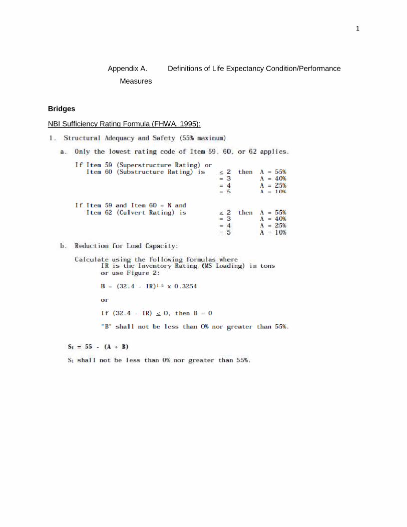
1
Appendix A. Definitions of Life Expectancy Condition/Performance
Measures
Bridges
NBI Sufficiency Rating Formula (FHWA, 1995):

2

3

4

5

6
NBI Deck, Superstructure, and Substructure Ratings (FHWA, 1995):
Code Description N NOT APPLICABLE 9 EXCELLENT CONDITION 8 VERY GOOD CONDITION - no problems noted. 7 GOOD CONDITION - some minor problems. 6 SATISFACTORY CONDITION - structural elements show some minor deterioration. 5 FAIR CONDITION - all primary structural elements are sound but may have minor
section loss, cracking, spalling or scour. 4 POOR CONDITION - advanced section loss, deterioration, spalling or scour. 3 SERIOUS CONDITION - loss of section, deterioration, spalling or scour have seriously
affected primary structural components. Local failures are possible. Fatigue cracks in steel or shear cracks in concrete may be present.
2 CRITICAL CONDITION - advanced deterioration of primary structural elements. Fatigue cracks in steel or shear cracks in concrete may be present or scour may have removed substructure support. Unless closely monitored it may be necessary to close the bridge until corrective action is taken.
1 "IMMINENT" FAILURE CONDITION - major deterioration or section loss present in critical structural components or obvious vertical or horizontal movement affecting structure stability. Bridge is closed to traffic but corrective action may put back in light service.
0 FAILED CONDITION - out of service - beyond corrective action.
NBI Channel/Channel Protection Rating (FHWA, 1995):
Code Description N Not applicable. Use when bridge is not over a waterway (channel). 9 There are no noticeable or noteworthy deficiencies which affect the condition of the
channel. 8 Banks are protected or well vegetated. River control devices such as spur dikes and
embankment protection are not required or are in a stable condition. 7 Bank protection is in need of minor repairs. River control devices and embankment
protection have a little minor damage. Banks and/or channel have minor amounts of drift.
6 Bank is beginning to slump. River control devices and embankment protection have widespread minor damage. There is minor stream bed movement evident. Debris is restricting the channel slightly.
5 Bank protection is being eroded. River control devices and/or embankment have major damage. Trees and brush restrict the channel.
4 Bank and embankment protection is severely undermined. River control devices have severe damage. Large deposits of debris are in the channel.
3 Bank protection has failed. River control devices have been destroyed. Stream bed aggradation, degradation or lateral movement has changed the channel to now threaten the bridge and/or approach roadway.
2 The channel has changed to the extent the bridge is near a state of collapse. 1 Bridge closed because of channel failure. Corrective action may put back in light service. 0 Bridge closed because of channel failure. Replacement necessary.

7
NBI Deck Geometry Rating (FHWA, 1995):
Rating taken as minimum of Table A-1 through Table A-3.
Table A-1: Deck Geometry Rating by Comparison of ADT to Bridge Roadway Width, Curb-to-Curb
Code
Bridge Roadway Width 2 Lanes: 2 Way Traffic
Bridge Roadway Width
1 Lane: 2-way Traffic
ADT (both directions) ADT (both directions)
0-100 101-400 401-1000 1001-2000 2001-5000 >5000 0-100 >100 9 >9.8 >11.0 >12.2 >13.4 >13.4 >13.4 -- -- 8 9.8 11.0 12.2 13.4 13.4 13.4 >4.9 -- 7 8.5 9.8 11.0 12.2 13.4 13.4 4.6 -- 6 7.3 8.5 9.1 10.4 12.2 13.4 4.3 -- 5 6.1 7.3 7.9 8.5 10.4 11.6 4.0 -- 4 5.5 6.1 6.7 7.3 8.5 9.8 (8.5)* 3.7 -- 3 4.9 5.5 6.1 6.7 7.9 9.1 (7.9)* 3.4 <4.9 2 Any width less than required for a rating code of 3 and structure is open 0 Bridge closed
*Use value in parenthesis for bridges longer than 60 meters
Table A-2: Deck Geometry Rating by Comparison of Number of Lanes to Bridge Roadway Width, Curb-to-Curb
Code
Bridge Roadway Width 2 or More Lanes
Bridge Roadway Width 1-way Traffic
Interstate and Other Divided Freeways Other Multilane Divided Facilities Ramps Only
2 Lanes 1-way 3 or more Lanes 2 Lanes 1-
way 3 or more Lanes 1 Lane 2 or more Lanes
9 >12.8 >3.7N+7.3 >12.8 >3.7N+5.5 >7.9 >3.7N+3.7 8 12.8 3.7N+7.3 12.8 3.7N+5.5 7.9 3.7N+3.7 7 12.2 3.7N+6.1 11.6 3.7N+4.6 7.3 3.7N+3.0 6 11.6 3.7N+4.9 11.0 3.7N+3.7 6.7 3.7N+2.4 5 11.0 3.7N+4.3 10.1 3.4N+3.0 6.1 3.7N+1.8
4 10.4 (8.8)* 3.4N+3.7 (3.4N+2.1)* 9.1 3.4N+1.8 5.5 3.7N+1.2
3 10.1 (8.5)* 3.4N+3.4
(3.4N+1.8)* 8.2 3.4N+1.5 4.9 3.7N+0.6
2 Any width less than required for a rating code of 3 and structure is open 0 Bridge closed
*Use value in parenthesis for bridges longer than 60 meters N = Total number of lanes of traffic on the structure.

8
Table A-3: Deck Geometry Rating by Comparison of Functional Class to Bridge Roadway Width, Curb-to-Curb
Code
Minimum Vertical Clearance Functional Class
Interstate and Other Freeway
Other Principal and Minor Arterial
Major and Minor Collectors and Locals
9 >5.18 >5.02 >5.02 8 5.18 5.02 5.02 7 5.10 4.72 4.72 6 5.02 4.41 4.41 5 4.80 4.34 4.34 4 4.57 4.26 4.26
3 Vertical clearance less than value in rating code of 4 and requiring corrective action.
2 Vertical clearance less than value in rating code of 4 and requiring replacement. 0 Bridge closed.
NBI Scour Protection Rating (FHWA, 1995):
Code Description N Bridge not over waterway. U Bridge with "unknown" foundation that has not been evaluated for scour. Since risk
cannot be determined, flag for monitoring during flood events and, if appropriate, closure.
T Bridge over "tidal" waters that has not been evaluated for scour, but considered low risk. Bridge will be monitored with regular inspection cycle and with appropriate underwater inspections. ("Unknown" foundations in "tidal" waters should be coded U.)
9 Bridge foundations (including piles) on dry land well above flood water elevations. 8 Bridge foundations determined to be stable for assessed or calculated scour conditions;
calculated scour is above top of footing. (Example A) 7 Countermeasures have been installed to correct a previously existing problem with
scour. Bridge is no longer scour critical. 6 Scour calculation/evaluation has not been made. (Use only to describe case where
bridge has not yet been evaluated for scour potential.) 5 Bridge foundations determined to be stable for calculated scour conditions; scour within
limits of footing or piles. (Example B) 4 Bridge foundations determined to be stable for calculated scour conditions; field review
indicates action is required to protect exposed foundations from effects of additional erosion and corrosion.
3 Bridge is scour critical; bridge foundations determined to be unstable for calculated scour conditions: - Scour within limits of footing or piles. (Example B) - Scour below spread-footing base or pile tips. (Example C)
2 Bridge is scour critical; field review indicates that extensive scour has occurred at bridge foundations. Immediate action is required to provide scour countermeasures.
1 Bridge is scour critical; field review indicates that failure of piers/abutments is imminent. Bridge is closed to traffic.
0 Bridge is scour critical. Bridge has failed and is closed to traffic.

9
EXAMPLES CALCULATED SCOUR DEPTH ACTION NEEDED

10
Box Culverts
NBI Culvert Rating (FHWA, 1995):
Code Description N Not applicable. Use if structure is not a culvert. 9 No deficiencies. 8 No noticeable or noteworthy deficiencies which affect the condition of the culvert.
Insignificant scrape marks caused by drift. 7 Shrinkage cracks, light scaling, and insignificant spalling which does not expose
reinforcing steel. Insignificant damage caused by drift with no misalignment and not requiring corrective action. Some minor scouring has occurred near curtain walls, wingwalls, or pipes. Metal culverts have a smooth symmetrical curvature with superficial corrosion and no pitting.
6 Deterioration or initial disintegration, minor chloride contamination, cracking with some leaching, or spalls on concrete or masonry walls and slabs. Local minor scouring at curtain walls, wingwalls, or pipes. Metal culverts have a smooth curvature, non-symmetrical shape, significant corrosion or moderate pitting.
5 Moderate to major deterioration or disintegration, extensive cracking and leaching, or spalls on concrete or masonry walls and slabs. Minor settlement or misalignment. Noticeable scouring or erosion at curtain walls, wingwalls, or pipes. Metal culverts have significant distortion and deflection in one section, significant corrosion or deep pitting.
4 Large spalls, heavy scaling, wide cracks, considerable efflorescence, or opened construction joint permitting loss of backfill. Considerable settlement or misalignment. Considerable scouring or erosion at curtain walls, wingwalls or pipes. Metal culverts have significant distortion and deflection throughout, extensive corrosion or deep pitting.
3 Any condition described in Code 4 but which is excessive in scope. Severe movement or differential settlement of the segments, or loss of fill. Holes may exist in walls or slabs. Integral wingwalls nearly severed from culvert. Severe scour or erosion at curtain walls, wingwalls or pipes. Metal culverts have extreme distortion and deflection in one section, extensive corrosion, or deep pitting with scattered perforations.
2 Integral wingwalls collapsed, severe settlement of roadway due to loss of fill. Section of culvert may have failed and can no longer support embankment. Complete undermining at curtain walls and pipes. Corrective action required to maintain traffic. Metal culverts have extreme distortion and deflection throughout with extensive perforations due to corrosion.
1 Culvert closed. Corrective action may put back in light service. 0 Culvert closed. Replacement necessary.

11
NBI Channel/Channel Protection Rating (FHWA, 1995):
Code Description N Not applicable. Use when box culvert is not over a waterway (channel). 9 There are no noticeable or noteworthy deficiencies which affect the condition of the
channel. 8 Banks are protected or well vegetated. River control devices such as spur dikes and
embankment protection are not required or are in a stable condition. 7 Bank protection is in need of minor repairs. River control devices and embankment
protection have a little minor damage. Banks and/or channel have minor amounts of drift.
6 Bank is beginning to slump. River control devices and embankment protection have widespread minor damage. There is minor stream bed movement evident. Debris is restricting the channel slightly.
5 Bank protection is being eroded. River control devices and/or embankment have major damage. Trees and brush restrict the channel.
4 Bank and embankment protection is severely undermined. River control devices have severe damage. Large deposits of debris are in the channel.
3 Bank protection has failed. River control devices have been destroyed. Stream bed aggradation, degradation or lateral movement has changed the channel to now threaten the box culvert and/or approach roadway.
2 The channel has changed to the extent the box culvert is near a state of collapse. 1 Box culvert closed because of channel failure. Corrective action may put back in light
service. 0 Box culvert closed because of channel failure. Replacement necessary.

12
Pipe Culverts
Pennsylvania DOT Pipe Culvert Physical Rating:
Code Description 0 Approaching original condition – like new, no defects 1 Discoloration, slight spalling of mortar, minor surface rust or scale which could include
minor pitting, slight loss of interior protection. 2 Moderate spalling and loss of mortar and/or aggregate, moderate to heavy rust and
pitting, significant loss of interior protection, weathered joints. 3 Extensive deterioration, rotted, perforated to completely deteriorated bottom, loss of
invert.
Pennsylvania DOT Pipe Culvert Structural Rating:
Code Description 0 No displacement, as installed, good condition. 1 Pipe sag or structural components displaced <20°. 2 Pipe sag or structural components displaced ≥20° joint separation, scouring. 3 Completely deteriorated, collapsed or failed.
Pennsylvania DOT Pipe Culvert Structural Rating:
Code Description 0 Open, no restriction of flow. 1 Minor flow restriction. Pipes or other structures are less than half clogged. Ditches have
minor siltation or clogging with stones or debris to less than half the cross-section. 2 Severe flow restriction. Pipes or structures are more than half to completely clogged.
Ditches are 50% or more filled with dirt, stones, debris or any other condition which causes the ditch to be non-functional due to inadequate slope.
3 Undetermined. Flow condition of pipe, structure or ditch cannot be determined due to excess vegetation.
4 Undetermined. Flow condition of pipe, structure or ditch cannot be determined due to inaccessibility.
5 Same as condition 0 with possible illicit discharge. 6 Same as condition 1 with possible illicit discharge. 7 Same as condition 2 with possible illicit discharge. 8 Same as condition 3 with possible illicit discharge. 9 Same as condition 4 with possible illicit discharge.

13
Appendix B. Bridge Markov/Weibull Results by Element, Region, and ‘Failure Mechanism’
Table B-1: Bridge Deck Element Markov/Weibull Results (End-of-Life Threshold: Deck Condition Rating = 3)
Region
Weibull Scaling
Factor, α
Weibull Shape
Factor, β
Median Service
Life
90% Confidence
Interval RMSE
Alabama 89.97 3.12 80 [35, 128] 6.40 Alaska 72.62 4.55 67 [38, 92] 10.20 Arizona 83.08 2.83 73 [29, 122] 5.55 Arkansas 100.46 10.46 97 [76, 112] 9.86 California 85.38 2.83 75 [30, 126] 4.43 Colorado 115.13 3.29 103 [47, 161] 10.02 Connecticut 97.59 5.24 91 [55, 120] 4.54 Delaware 60.81 5.67 57 [36, 74] 3.25 Florida 87.01 15.68 85 [72, 93] 7.97 Georgia 131.29 2.96 116 [48, 190] 5.82 Hawaii 110.47 27.27 109 [99, 115] 8.67 Idaho 92.49 5.04 86 [51, 115] 6.83 Illinois 109.67 2.98 97 [41, 158] 1.84 Indiana 88.95 3.46 80 [38, 122] 1.95 Iowa 89.75 3.57 81 [39, 122] 2.62 Kansas 104.13 5.17 97 [59, 129] 1.85 Kentucky 67.77 3.01 60 [25, 98] 3.31 Louisiana 104.20 5.12 97 [58, 129] 8.03 Maine 76.88 3.39 69 [32, 106] 2.38 Maryland 85.10 14.67 83 [70, 92] 21.15 Massachusetts 67.34 3.17 60 [26, 95] 3.29 Michigan 73.32 3.04 65 [28, 105] 1.56 Minnesota 80.97 14.88 79 [66, 87] 16.24 Mississippi 109.57 4.01 100 [52, 144] 7.51 Missouri 91.07 2.83 80 [32, 134] 3.77 Montana 96.11 3.68 87 [43, 129] 5.15 Nebraska 109.05 7.73 104 [74, 126] 2.35 Nevada 75.66 5.77 71 [45, 92] 5.41 New Hampshire 83.70 2.98 74 [31, 121] 5.31 New Jersey 113.43 9.21 109 [82, 128] 11.01

14
Table B-1: Continued
Region
Weibull Scaling
Factor, α
Weibull Shape
Factor, β
Median Service
Life
90% Confidence
Interval RMSE
New Mexico 86.05 3.73 78 [39, 115] 5.73 New York 81.57 3.30 73 [33, 114] 0.89 North Carolina 93.09 31.02 92 [85, 96] 7.49 North Dakota N/A N/A >120 N/A N/A Ohio 57.75 2.95 51 [21, 84] 1.15 Oklahoma 54.86 3.24 49 [22, 77] 3.29 Oregon 80.97 14.88 79 [66, 87] 14.75 Pennsylvania 84.68 3.39 76 [35, 117] 1.96 Rhode Island 77.76 2.73 68 [26, 116] 3.33 South Carolina 100.16 4.31 92 [50, 129] 7.24 South Dakota 69.64 3.15 62 [27, 99] 3.20 Tennessee 109.07 19.17 107 [93, 115] 4.61 Texas 105.19 2.97 93 [39, 152] 5.97 Utah 77.96 14.36 76 [63, 84] 20.14 Vermont 65.67 2.95 58 [24, 95] 1.75 Virginia 108.53 3.99 99 [52, 143] 5.30 Washington 114.18 3.56 103 [50, 155] 7.21 West Virginia 86.67 3.10 77 [33, 124] 2.69 Wisconsin 72.66 2.89 64 [26, 106] 4.46 Wyoming 61.12 2.96 54 [22, 89] 1.99
Entire U.S. 88.33 3.28 79 [36, 123] 0.89 Northeast U.S. 81.22 3.04 72 [31, 117] 1.09 Northwest U.S. 102.86 4.61 95 [54, 130] 3.29 Southeast U.S. 92.60 4.28 85 [46, 120] 3.01 Southwest U.S. 93.37 3.47 84 [40, 128] 4.98
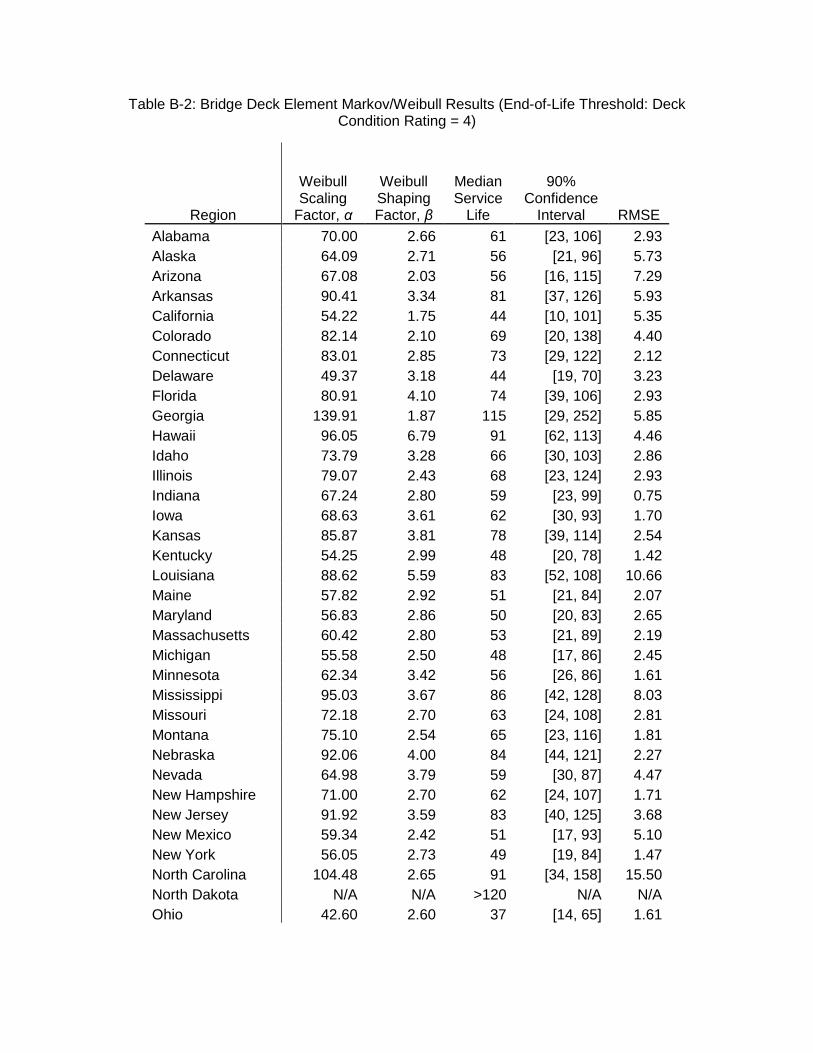
15
Table B-2: Bridge Deck Element Markov/Weibull Results (End-of-Life Threshold: Deck Condition Rating = 4)
Region
Weibull Scaling
Factor, α
Weibull Shaping Factor, β
Median Service
Life
90% Confidence
Interval RMSE
Alabama 70.00 2.66 61 [23, 106] 2.93 Alaska 64.09 2.71 56 [21, 96] 5.73 Arizona 67.08 2.03 56 [16, 115] 7.29 Arkansas 90.41 3.34 81 [37, 126] 5.93 California 54.22 1.75 44 [10, 101] 5.35 Colorado 82.14 2.10 69 [20, 138] 4.40 Connecticut 83.01 2.85 73 [29, 122] 2.12 Delaware 49.37 3.18 44 [19, 70] 3.23 Florida 80.91 4.10 74 [39, 106] 2.93 Georgia 139.91 1.87 115 [29, 252] 5.85 Hawaii 96.05 6.79 91 [62, 113] 4.46 Idaho 73.79 3.28 66 [30, 103] 2.86 Illinois 79.07 2.43 68 [23, 124] 2.93 Indiana 67.24 2.80 59 [23, 99] 0.75 Iowa 68.63 3.61 62 [30, 93] 1.70 Kansas 85.87 3.81 78 [39, 114] 2.54 Kentucky 54.25 2.99 48 [20, 78] 1.42 Louisiana 88.62 5.59 83 [52, 108] 10.66 Maine 57.82 2.92 51 [21, 84] 2.07 Maryland 56.83 2.86 50 [20, 83] 2.65 Massachusetts 60.42 2.80 53 [21, 89] 2.19 Michigan 55.58 2.50 48 [17, 86] 2.45 Minnesota 62.34 3.42 56 [26, 86] 1.61 Mississippi 95.03 3.67 86 [42, 128] 8.03 Missouri 72.18 2.70 63 [24, 108] 2.81 Montana 75.10 2.54 65 [23, 116] 1.81 Nebraska 92.06 4.00 84 [44, 121] 2.27 Nevada 64.98 3.79 59 [30, 87] 4.47 New Hampshire 71.00 2.70 62 [24, 107] 1.71 New Jersey 91.92 3.59 83 [40, 125] 3.68 New Mexico 59.34 2.42 51 [17, 93] 5.10 New York 56.05 2.73 49 [19, 84] 1.47 North Carolina 104.48 2.65 91 [34, 158] 15.50 North Dakota N/A N/A >120 N/A N/A Ohio 42.60 2.60 37 [14, 65] 1.61

16
Table B-2: Continued
Region
Weibull Scaling
Factor, α
Weibull Shaping Factor, β
Median Service
Life
90% Confidence
Interval RMSE
Oklahoma 43.91 3.09 39 [17, 63] 2.87 Oregon 70.41 3.30 63 [29, 98] 1.75 Pennsylvania 61.12 2.57 53 [19, 94] 1.05 Rhode Island 54.37 2.52 47 [17, 84] 2.13 South Carolina 82.09 14.19 80 [67, 89] 22.13 South Dakota 55.11 2.65 48 [18, 83] 3.56 Tennessee 117.78 3.48 106 [50, 161] 6.45 Texas 78.59 2.82 69 [27, 116] 2.21 Utah 69.81 2.42 60 [20, 110] 2.74 Vermont 53.42 2.86 47 [19, 78] 0.99 Virginia 64.03 2.73 56 [22, 96] 1.97 Washington 72.76 9.47 70 [53, 82] 19.22 West Virginia 63.24 2.32 54 [18, 101] 4.19 Wisconsin 52.44 2.80 46 [18, 78] 2.46 Wyoming 47.34 2.18 40 [12, 78] 3.76
Entire U.S. 66.44 2.70 58 [22, 100] 1.17 Northeast U.S. 58.61 2.63 51 [19, 89] 1.58 Northwest U.S. 82.79 3.27 74 [33, 116] 1.70 Southeast U.S. 75.69 3.42 68 [32, 104] 1.46 Southwest U.S. 68.58 2.19 58 [18, 113] 2.81

17
Table B-3: Bridge Deck Element Markov/Weibull Results (End-of-Life Threshold: Deck Condition Rating = 5)
Region
Weibull Scaling
Factor, α
Weibull Shaping Factor, β
Median Service
Life
90% Confidence
Interval RMSE
Alabama 47.52 2.48 41 [14, 74] 1.18 Alaska 28.30 2.22 24 [7, 46] 3.72 Arizona 50.49 2.28 43 [14, 82] 1.75 Arkansas 64.42 1.88 53 [13, 116] 3.17 California 37.71 1.87 31 [8, 68] 3.45 Colorado 57.22 2.09 48 [14, 97] 1.91 Connecticut 62.74 2.17 53 [16, 104] 4.13 Delaware 39.95 2.77 35 [14, 59] 2.74 Florida 74.58 2.66 65 [24, 113] 3.98 Georgia 82.66 2.03 69 [19, 142] 4.63 Hawaii 75.23 3.16 67 [29, 106] 2.91 Idaho 58.60 2.64 51 [19, 89] 2.78 Illinois 60.75 2.36 52 [17, 97] 2.09 Indiana 44.29 2.39 38 [13, 70] 0.74 Iowa 49.00 3.41 44 [20, 68] 1.24 Kansas 59.17 2.84 52 [21, 87] 1.05 Kentucky 43.33 2.79 38 [15, 64] 1.66 Louisiana 71.72 3.22 64 [29, 101] 2.58 Maine 45.55 2.82 40 [16, 67] 1.01 Maryland 42.55 2.62 37 [14, 65] 1.07 Massachusetts 44.34 2.37 38 [13, 70] 1.74 Michigan 40.78 2.40 35 [12, 64] 2.75 Minnesota 48.30 3.16 43 [19, 68] 0.98 Mississippi 72.01 2.74 63 [24, 107] 2.51 Missouri 53.62 2.78 47 [18, 80] 2.64 Montana 53.24 2.18 45 [14, 88] 1.33 Nebraska 60.43 3.26 54 [24, 85] 1.18 Nevada 55.19 3.08 49 [21, 79] 8.92 New Hampshire 53.04 2.23 45 [14, 87] 2.16 New Jersey 60.99 2.30 52 [17, 98] 2.29 New Mexico 42.51 2.64 37 [14, 64] 1.74 New York 39.84 2.31 34 [11, 64] 2.16 North Carolina 58.71 2.03 49 [14, 101] 3.71 North Dakota 102.66 3.04 91 [39, 147] 3.98 Ohio 32.74 2.34 28 [9, 52] 1.88

18
Table B-3: Continued
Region
Weibull Scaling
Factor, α
Weibull Shaping Factor, β
Median Service
Life
90% Confidence
Interval RMSE
Oklahoma 31.64 3.00 28 [12, 46] 1.33 Oregon 53.62 2.78 47 [18, 80] 1.22 Pennsylvania 39.62 2.40 34 [11, 63] 1.72 Rhode Island 40.09 2.70 35 [13, 60] 1.93 South Carolina 54.42 2.92 48 [20, 79] 2.52 South Dakota 39.97 2.76 35 [14, 59] 1.47 Tennessee 86.64 2.14 73 [22, 145] 4.00 Texas 57.16 2.38 49 [16, 91] 1.85 Utah 51.43 2.05 43 [12, 88] 2.81 Vermont 40.44 2.54 35 [13, 62] 0.54 Virginia 37.25 2.41 32 [11, 59] 1.22 Washington 64.69 2.26 55 [17, 105] 2.93 West Virginia 46.22 2.53 40 [14, 71] 2.52 Wisconsin 37.94 2.63 33 [12, 58] 1.82 Wyoming 28.71 2.05 24 [7, 49] 2.98
Entire U.S. 48.62 2.50 42 [15, 75] 0.99 Northeast U.S. 42.73 2.54 37 [13, 66] 1.17 Northwest U.S. 56.02 2.74 49 [19, 84] 0.77 Southeast U.S. 57.04 2.78 50 [20, 85] 0.72 Southwest U.S. 47.06 1.95 39 [10, 83] 2.23

19
Table B-4: Bridge Superstructure Element Markov/Weibull Results (End-of-Life Threshold: Superstructure Condition Rating = 3)
Region
Weibull Scaling
Factor, α
Weibull Shaping Factor, β
Median Service
Life
90% Confidence
Interval RMSE
Alabama 86.10 14.84 84 [70, 93] 20.66 Alaska 63.50 9.12 61 [46, 72] 14.96 Arizona 80.97 14.88 79 [66, 87] 11.85 Arkansas 97.18 8.33 93 [68, 111] 5.39 California 112.94 10.31 109 [85, 126] 6.78 Colorado 102.36 11.00 99 [78, 113] 7.29 Connecticut 105.80 4.22 97 [52, 137] 4.02 Delaware 57.36 8.72 55 [41, 65] 13.96 Florida 88.21 9.88 85 [65, 99] 8.34 Georgia 126.68 4.16 116 [62, 165] 5.21 Hawaii 97.14 6.74 92 [63, 114] 4.59 Idaho 91.03 6.44 86 [57, 108] 7.39 Illinois 113.46 3.15 101 [44, 161] 0.79 Indiana 89.70 3.59 81 [39, 122] 1.37 Iowa 90.23 14.65 88 [74, 97] 14.71 Kansas 102.75 7.75 98 [70, 118] 2.36 Kentucky 82.45 3.39 74 [34, 114] 2.76 Louisiana 116.13 5.79 109 [70, 140] 9.23 Maine 87.33 3.66 79 [39, 118] 3.14 Maryland 88.57 3.60 80 [39, 120] 3.68 Massachusetts 72.92 2.51 63 [22, 113] 3.88 Michigan 75.36 3.56 68 [33, 103] 2.07 Minnesota 82.66 3.77 75 [38, 111] 1.51 Mississippi 118.83 3.21 106 [47, 167] 7.57 Missouri 110.87 4.40 102 [56, 142] 4.79 Montana 119.94 8.71 115 [85, 136] 9.80 Nebraska 112.18 7.75 107 [76, 129] 3.86 Nevada 78.20 5.33 73 [45, 96] 6.59 New Hampshire 106.28 3.27 95 [43, 149] 5.13 New Jersey 122.32 5.94 115 [74, 147] 6.51 New Mexico 88.08 3.81 80 [40, 118] 3.07 New York 73.69 3.33 66 [30, 102] 1.53 North Carolina 100.11 11.62 97 [78, 110] 9.27 North Dakota N/A N/A >120 N/A N/A Ohio 58.98 2.91 52 [21, 86] 0.83

20
Table B-4: Continued
Region
Weibull Scaling
Factor, α
Weibull Shaping Factor, β
Median Service
Life
90% Confidence
Interval RMSE
Oklahoma 57.29 3.78 52 [26, 77] 2.15 Oregon 125.40 1.86 103 [25, 226] 8.63 Pennsylvania 89.87 3.53 81 [39, 123] 2.45 Rhode Island 72.45 2.35 62 [20, 116] 3.75 South Carolina 118.87 4.23 109 [59, 154] 9.30 South Dakota 84.72 3.38 76 [35, 117] 2.50 Tennessee 109.38 106.58 109 [106, 111] 8.57 Texas 94.67 3.81 86 [43, 126] 3.08 Utah 121.56 3.36 109 [50, 169] 7.02 Vermont 78.41 3.23 70 [31, 110] 1.39 Virginia 102.03 2.92 90 [37, 149] 2.30 Washington 108.76 4.95 101 [60, 136] 6.35 West Virginia 100.91 2.92 89 [36, 147] 2.19 Wisconsin 78.67 3.57 71 [34, 107] 2.52 Wyoming 78.97 14.53 77 [64, 85] 18.59
Entire U.S. 91.97 3.57 83 [40, 125] 1.08 Northeast U.S. 85.19 3.21 76 [34, 120] 0.97 Northwest U.S. 104.81 6.43 99 [66, 124] 2.46 Southeast U.S. 88.15 4.33 81 [44, 114] 1.55 Southwest U.S. 103.27 3.50 93 [44, 141] 3.44

21
Table B-5: Bridge Superstructure Element Markov/Weibull Results (End-of-Life Threshold: Superstructure Condition Rating = 4)
Region
Weibull Scaling
Factor, α
Weibull Shaping Factor, β
Median Service
Life
90% Confidence
Interval RMSE
Alabama 73.14 2.46 63 [22, 114] 3.28 Alaska 59.59 8.25 57 [42, 68] 16.01 Arizona 68.63 9.36 66 [50, 77] 16.04 Arkansas 88.90 4.54 82 [46, 113] 6.12 California 104.54 4.30 96 [52, 135] 2.40 Colorado 78.97 14.53 77 [64, 85] 16.62 Connecticut 90.45 2.98 80 [33, 131] 1.84 Delaware 42.87 3.04 38 [16, 62] 2.47 Florida 80.53 5.15 75 [45, 100] 4.63 Georgia 135.44 2.24 115 [36, 221] 5.70 Hawaii 83.23 3.52 75 [36, 114] 6.26 Idaho 76.61 3.50 69 [33, 105] 2.38 Illinois 84.72 2.71 74 [28, 127] 3.10 Indiana 69.29 3.30 62 [28, 97] 1.10 Iowa 78.83 3.51 71 [34, 108] 2.11 Kansas 89.52 4.85 83 [49, 112] 2.56 Kentucky 63.31 2.99 56 [23, 91] 1.28 Louisiana 95.00 3.30 85 [39, 133] 6.28 Maine 72.93 3.18 65 [29, 103] 2.00 Maryland 65.69 2.95 58 [24, 95] 1.61 Massachusetts 62.29 2.57 54 [20, 96] 2.25 Michigan 61.96 3.08 55 [24, 89] 1.49 Minnesota 60.10 3.42 54 [25, 83] 2.39 Mississippi 93.46 3.86 85 [43, 124] 7.10 Missouri 92.17 3.13 82 [36, 131] 2.22 Montana 103.50 3.11 92 [40, 147] 3.11 Nebraska 97.96 5.84 92 [59, 118] 2.72 Nevada 65.89 3.91 60 [31, 87] 7.23 New Hampshire 91.92 2.90 81 [33, 134] 3.47 New Jersey 102.43 3.80 93 [47, 137] 2.00 New Mexico 72.46 2.35 62 [20, 116] 4.77 New York 57.75 2.95 51 [21, 84] 1.66 North Carolina 78.97 14.53 77 [64, 85] 18.67 North Dakota 113.99 10.29 110 [85, 127] 5.58 Ohio 48.93 2.84 43 [17, 72] 0.98

22
Table B-5: Continued
Region
Weibull Scaling
Factor, α
Weibull Shaping Factor, β
Median Service
Life
90% Confidence
Interval RMSE
Oklahoma 48.18 3.22 43 [19, 68] 1.98 Oregon 71.61 2.86 63 [25, 105] 1.86 Pennsylvania 64.77 2.87 57 [23, 95] 1.11 Rhode Island 44.85 2.21 38 [12, 74] 2.01 South Carolina 71.97 2.75 63 [24, 107] 6.81 South Dakota 68.21 2.86 60 [24, 100] 1.69 Tennessee 108.31 4.59 100 [57, 138] 8.06 Texas 77.36 3.21 69 [31, 109] 1.28 Utah 82.37 3.04 73 [31, 118] 2.45 Vermont 61.90 3.10 55 [24, 88] 2.10 Virginia 59.48 3.18 53 [23, 84] 1.63 Washington 78.97 14.53 77 [64, 85] 19.08 West Virginia 79.18 2.66 69 [26, 120] 1.80 Wisconsin 61.68 3.20 55 [24, 87] 1.73 Wyoming 67.85 3.44 61 [29, 93] 2.32
Entire U.S. 72.26 3.02 64 [27, 104] 0.76 Northeast U.S. 64.76 2.87 57 [23, 95] 1.25 Northwest U.S. 87.66 4.01 80 [42, 115] 1.72 Southeast U.S. 76.71 3.46 69 [33, 105] 0.85 Southwest U.S. 86.80 3.43 78 [37, 120] 2.10

23
Table B-6: Bridge Superstructure Element Markov/Weibull Results (End-of-Life Threshold: Superstructure Condition Rating = 5)
Region
Weibull Scaling
Factor, α
Weibull Shaping Factor, β
Median Service
Life
90% Confidence
Interval RMSE
Alabama 51.19 2.42 44 [15, 81] 1.43 Alaska 29.45 2.24 25 [8, 48] 2.30 Arizona 58.82 2.57 51 [19, 90] 3.17 Arkansas 69.04 1.91 57 [15, 122] 2.05 California 77.95 2.68 68 [26, 117] 3.06 Colorado 61.99 2.34 53 [17, 99] 2.19 Connecticut 68.69 2.41 59 [20, 108] 1.20 Delaware 33.60 2.49 29 [10, 52] 1.21 Florida 69.57 3.18 62 [27, 98] 3.06 Georgia 75.68 2.41 65 [22, 119] 4.79 Hawaii 71.42 2.92 63 [26, 104] 5.52 Idaho 60.16 2.89 53 [22, 88] 1.61 Illinois 64.94 2.47 56 [20, 101] 1.80 Indiana 52.14 2.93 46 [19, 76] 0.79 Iowa 58.12 3.29 52 [24, 81] 0.78 Kansas 67.14 3.26 60 [27, 94] 1.47 Kentucky 52.34 2.84 46 [18, 77] 1.28 Louisiana 73.26 3.06 65 [28, 105] 2.45 Maine 59.44 3.20 53 [23, 84] 2.01 Maryland 42.78 2.53 37 [13, 66] 1.15 Massachusetts 47.04 2.26 40 [13, 76] 1.07 Michigan 46.10 2.58 40 [15, 71] 1.50 Minnesota 48.33 3.14 43 [19, 69] 0.83 Mississippi 68.56 2.75 60 [23, 102] 2.30 Missouri 69.11 2.94 61 [25, 100] 1.19 Montana 72.66 2.57 63 [23, 111] 2.42 Nebraska 78.46 3.67 71 [35, 106] 1.94 Nevada 59.45 3.81 54 [27, 79] 4.40 New Hampshire 71.09 2.40 61 [21, 112] 1.23 New Jersey 71.01 3.06 63 [27, 102] 1.47 New Mexico 48.69 2.48 42 [15, 76] 1.94 New York 45.00 2.56 39 [14, 69] 1.78 North Carolina 63.26 2.32 54 [18, 102] 5.30 North Dakota 120.19 3.75 109 [54, 161] 5.34 Ohio 38.45 2.40 33 [11, 61] 1.15

24
Table B-6: Continued
Region
Weibull Scaling
Factor, α
Weibull Shaping Factor, β
Median Service
Life
90% Confidence
Interval RMSE
Oklahoma 35.33 2.80 31 [12, 52] 0.92 Oregon 54.03 2.63 47 [17, 82] 1.16 Pennsylvania 44.61 2.73 39 [15, 67] 1.07 Rhode Island 28.11 2.32 24 [8, 45] 1.48 South Carolina 53.41 3.43 48 [22, 74] 2.32 South Dakota 47.95 2.77 42 [16, 71] 1.05 Tennessee 81.98 2.55 71 [26, 126] 3.28 Texas 58.14 2.43 50 [17, 91] 0.65 Utah 65.29 2.39 56 [19, 103] 2.38 Vermont 46.85 2.75 41 [16, 70] 1.39 Virginia 40.99 2.82 36 [14, 60] 0.93 Washington 64.31 2.65 56 [21, 97] 1.53 West Virginia 58.96 2.22 50 [15, 97] 1.97 Wisconsin 46.25 3.04 41 [17, 66] 0.98 Wyoming 49.00 2.38 42 [14, 78] 2.29
Entire U.S. 55.03 2.68 48 [18, 83] 0.67 Northeast U.S. 48.33 2.61 42 [16, 74] 0.99 Northwest U.S. 64.53 2.95 57 [24, 94] 0.88 Southeast U.S. 59.34 2.78 52 [20, 88] 0.81 Southwest U.S. 62.45 2.52 54 [19, 96] 0.71

25
Table B-7: Bridge Substructure Element Markov/Weibull Results (End-of-Life Threshold: Substructure Condition Rating = 3)
Region
Weibull Scaling
Factor, α
Weibull Shaping Factor, β
Median Service
Life
90% Confidence
Interval RMSE
Alabama 87.51 2.19 74 [22, 145] 4.67 Alaska 71.39 5.77 67 [43, 86] 10.77 Arizona 80.97 14.88 79 [66, 87] 15.52 Arkansas 100.38 5.58 94 [59, 122] 9.95 California 113.51 9.04 109 [82, 128] 6.54 Colorado 101.99 4.49 94 [53, 130] 6.91 Connecticut 123.96 2.85 109 [44, 182] 11.60 Delaware 68.08 4.73 63 [36, 86] 4.99 Florida 90.65 6.96 86 [59, 106] 8.00 Georgia 114.65 3.42 103 [48, 158] 14.86 Hawaii 104.91 19.90 103 [90, 111] 7.53 Idaho 80.97 14.88 79 [66, 87] 17.19 Illinois 118.45 3.30 106 [48, 165] 1.28 Indiana 90.96 3.54 82 [39, 124] 1.37 Iowa 71.60 3.27 64 [29, 100] 3.50 Kansas 101.22 4.33 93 [51, 130] 1.42 Kentucky 84.44 3.09 75 [32, 120] 3.01 Louisiana 95.77 5.00 89 [53, 119] 4.73 Maine 80.20 3.01 71 [30, 116] 2.85 Maryland 99.84 3.96 91 [47, 132] 7.96 Massachusetts 79.58 3.21 71 [32, 112] 4.02 Michigan 86.30 3.21 77 [34, 121] 2.33 Minnesota 75.30 3.14 67 [29, 107] 2.69 Mississippi 112.49 2.17 95 [29, 187] 7.40 Missouri 108.44 4.52 100 [56, 138] 7.38 Montana 144.23 1.62 115 [23, 284] 10.21 Nebraska 108.50 8.65 104 [77, 123] 3.31 Nevada 77.18 6.58 73 [49, 91] 7.34 New Hampshire 120.44 3.67 109 [54, 162] 4.72 New Jersey 116.90 22.42 115 [102, 123] 7.27 New Mexico 80.89 4.12 74 [39, 106] 6.89 New York 71.21 2.99 63 [26, 103] 1.36 North Carolina 101.67 7.79 97 [69, 117] 8.42 North Dakota 117.75 15.53 115 [97, 126] 6.80 Ohio 64.94 3.24 58 [26, 91] 0.84

26
Table B-7: Continued
Region
Weibull Scaling
Factor, α
Weibull Shaping Factor, β
Median Service
Life
90% Confidence
Interval RMSE
Oklahoma 45.71 3.37 41 [19, 63] 1.92 Oregon 65.84 8.31 63 [46, 75] 16.12 Pennsylvania 92.05 3.54 83 [40, 125] 0.86 Rhode Island 76.27 3.20 68 [30, 108] 5.31 South Carolina 105.88 2.61 92 [34, 161] 6.13 South Dakota 67.10 3.28 60 [27, 94] 1.67 Tennessee 113.40 9.27 109 [82, 128] 7.24 Texas 77.67 3.10 69 [30, 111] 1.38 Utah 100.91 4.49 93 [52, 129] 6.09 Vermont 78.71 2.51 68 [24, 122] 3.48 Virginia N/A N/A >120 N/A N/A Washington 124.27 2.80 109 [43, 184] 10.10 West Virginia 119.57 3.04 106 [45, 172] 1.79 Wisconsin 83.66 3.35 75 [35, 116] 3.60 Wyoming 82.18 3.09 73 [31, 117] 5.33
Entire U.S. 87.62 3.15 78 [34, 124] 0.91 Northeast U.S. 85.35 3.16 76 [33, 121] 1.14 Northwest U.S. 100.40 3.73 91 [45, 135] 1.06 Southeast U.S. 82.28 3.46 74 [35, 113] 1.66 Southwest U.S. 94.83 3.02 84 [35, 136] 2.11

27
Table B-8: Bridge Substructure Element Markov/Weibull Results (End-of-Life Threshold: Substructure Condition Rating = 4)
Region
Weibull Scaling
Factor, α
Weibull Shaping Factor, β
Median Service
Life
90% Confidence
Interval RMSE
Alabama 63.28 2.07 53 [15, 108] 3.34 Alaska 60.23 2.87 53 [21, 88] 6.11 Arizona 69.75 9.11 67 [50, 79] 18.65 Arkansas 79.97 14.71 78 [65, 86] 25.19 California 111.90 4.42 103 [57, 143] 6.95 Colorado 81.80 2.35 70 [23, 130] 3.02 Connecticut 86.53 3.14 77 [34, 123] 1.48 Delaware 48.82 2.89 43 [17, 71] 2.50 Florida 97.21 2.73 85 [33, 145] 9.75 Georgia 100.51 3.01 89 [37, 145] 11.71 Hawaii 104.20 4.47 96 [54, 133] 5.72 Idaho 68.06 3.35 61 [28, 94] 3.44 Illinois 79.97 14.71 78 [65, 86] 19.85 Indiana 73.10 3.12 65 [28, 104] 1.58 Iowa 57.67 3.54 52 [25, 79] 3.06 Kansas 83.62 3.84 76 [39, 111] 1.95 Kentucky 65.16 2.74 57 [22, 97] 1.20 Louisiana 87.95 3.05 78 [33, 126] 6.67 Maine 65.15 2.74 57 [22, 97] 1.54 Maryland 69.12 2.32 59 [19, 111] 3.76 Massachusetts 62.98 2.38 54 [18, 100] 2.25 Michigan 69.86 2.70 61 [23, 105] 1.23 Minnesota 60.11 3.42 54 [25, 83] 1.29 Mississippi 82.06 2.53 71 [25, 127] 5.94 Missouri 82.68 3.31 74 [34, 115] 1.86 Montana 78.78 2.49 68 [24, 122] 3.40 Nebraska 99.30 4.20 91 [49, 129] 2.60 Nevada 66.16 3.20 59 [26, 93] 4.03 New Hampshire 99.86 2.45 86 [30, 156] 3.20 New Jersey 105.78 2.85 93 [37, 156] 1.31 New Mexico 60.10 2.92 53 [22, 88] 1.11 New York 48.83 2.43 42 [14, 77] 2.15 North Carolina 79.50 2.59 69 [25, 122] 4.76 North Dakota 117.04 5.15 109 [66, 145] 5.25 Ohio 50.94 2.95 45 [19, 74] 1.09

28
Table B-8: Continued
Region
Weibull Scaling
Factor, α
Weibull Shaping Factor, β
Median Service
Life
90% Confidence
Interval RMSE
Oklahoma 36.44 2.82 32 [13, 54] 1.16 Oregon 57.68 2.56 50 [18, 88] 2.93 Pennsylvania 65.11 2.75 57 [22, 97] 0.72 Rhode Island 45.86 2.68 40 [15, 69] 3.74 South Carolina 52.33 8.03 50 [36, 60] 14.63 South Dakota 54.51 2.88 48 [19, 80] 1.32 Tennessee 115.10 3.03 102 [43, 165] 5.53 Texas 63.38 2.58 55 [20, 97] 0.92 Utah 99.27 2.19 84 [26, 164] 5.27 Vermont 54.87 2.37 47 [16, 87] 2.96 Virginia 75.91 2.36 65 [22, 121] 3.52 Washington 78.89 2.74 69 [27, 118] 3.39 West Virginia 95.17 2.46 82 [28, 149] 1.96 Wisconsin 64.35 3.53 58 [28, 88] 3.77 Wyoming 63.73 2.49 55 [19, 99] 2.21
Entire U.S. 67.36 2.77 59 [23, 100] 1.21 Northeast U.S. 63.90 2.78 56 [22, 95] 1.68 Northwest U.S. 78.42 3.23 70 [31, 110] 0.84 Southeast U.S. 65.90 2.87 58 [23, 97] 1.08 Southwest U.S. 76.32 2.28 65 [21, 123] 2.65

29
Table B-9: Bridge Substructure Element Markov/Weibull Results (End-of-Life Threshold: Substructure Condition Rating = 5)
Region
Weibull Scaling
Factor, α
Weibull Shaping Factor, β
Median Service
Life
90% Confidence
Interval RMSE
Alabama 49.41 2.26 42 [13, 80] 1.54 Alaska 29.60 2.17 25 [8, 49] 1.03 Arizona 65.59 2.61 57 [21, 100] 2.56 Arkansas 63.23 1.70 51 [11, 120] 3.92 California 79.97 14.71 78 [65, 86] 18.46 Colorado 59.53 1.88 49 [12, 107] 2.95 Connecticut 64.56 2.29 55 [18, 104] 1.10 Delaware 34.30 2.74 30 [12, 51] 1.90 Florida 71.01 2.41 61 [21, 112] 2.85 Georgia 63.57 2.25 54 [17, 104] 3.26 Hawaii 74.22 3.58 67 [32, 101] 2.54 Idaho 52.45 2.79 46 [18, 78] 1.46 Illinois 66.04 2.49 57 [20, 103] 1.89 Indiana 54.92 2.72 48 [18, 82] 0.57 Iowa 47.67 3.56 43 [21, 65] 1.25 Kansas 62.82 3.19 56 [25, 89] 0.78 Kentucky 50.87 2.53 44 [16, 79] 0.47 Louisiana 70.21 2.61 61 [22, 107] 2.84 Maine 50.60 2.62 44 [16, 77] 0.95 Maryland 45.66 2.33 39 [13, 73] 1.06 Massachusetts 40.56 2.08 34 [10, 69] 2.55 Michigan 50.69 2.23 43 [13, 83] 2.28 Minnesota 49.09 3.35 44 [20, 68] 0.84 Mississippi 67.75 2.12 57 [17, 114] 3.19 Missouri 62.15 3.00 55 [23, 90] 1.43 Montana 56.13 2.34 48 [16, 90] 1.01 Nebraska 76.34 3.62 69 [34, 103] 1.86 Nevada 64.22 2.68 56 [21, 97] 3.55 New Hampshire 74.16 2.05 62 [17, 127] 2.47 New Jersey 66.65 2.64 58 [22, 101] 1.58 New Mexico 39.33 2.52 34 [12, 61] 1.35 New York 37.61 2.27 32 [10, 61] 2.23 North Carolina 57.71 1.99 48 [13, 100] 5.56 North Dakota 99.18 4.26 91 [49, 128] 5.81 Ohio 39.49 2.45 34 [12, 62] 0.96

30
Table B-9: Continued
Region
Weibull Scaling
Factor, α
Weibull Shaping Factor, β
Median Service
Life
90% Confidence
Interval RMSE
Oklahoma 28.20 2.27 24 [8, 46] 1.27 Oregon 46.16 2.56 40 [14, 71] 1.34 Pennsylvania 41.27 2.22 35 [11, 68] 1.01 Rhode Island 29.68 2.13 25 [7, 50] 2.83 South Carolina 44.58 3.38 40 [19, 62] 3.22 South Dakota 40.95 2.33 35 [11, 66] 1.88 Tennessee 84.29 2.33 72 [23, 135] 2.86 Texas 47.12 2.24 40 [12, 77] 1.33 Utah 67.79 2.11 57 [17, 114] 3.00 Vermont 39.21 2.57 34 [12, 60] 1.59 Virginia 42.44 2.23 36 [11, 69] 1.97 Washington 60.96 2.62 53 [20, 93] 1.63 West Virginia 64.68 1.84 53 [13, 117] 4.20 Wisconsin 51.57 3.21 46 [20, 73] 1.03 Wyoming 45.50 2.03 38 [11, 78] 1.30
Entire U.S. 51.84 2.59 45 [16, 79] 0.77 Northeast U.S. 48.24 2.65 42 [16, 73] 0.81 Northwest U.S. 60.08 2.92 53 [22, 87] 0.66 Southeast U.S. 53.16 2.53 46 [16, 82] 0.71 Southwest U.S. 55.93 2.11 47 [14, 94] 1.01

31
Table B-10: Bridge Channel/Embankment Protection Markov/Weibull Results (End-of-Life Threshold: Channel Condition Rating = 3)
Region
Weibull Scaling
Factor, α
Weibull Shaping Factor, β
Median Service
Life
90% Confidence
Interval RMSE
Alabama 113.24 3.87 103 [53, 150] 9.15 Alaska 76.17 12.70 74 [60, 83] 8.41 Arizona 80.97 14.88 79 [66, 87] 14.11 Arkansas 106.22 17.36 104 [90, 113] 10.17 California N/A N/A >120 N/A N/A Colorado 101.38 15.46 99 [84, 109] 8.05 Connecticut 120.15 3.76 109 [55, 161] 4.75 Delaware 60.38 9.13 58 [44, 68] 10.93 Florida 92.48 22.78 91 [81, 97] 8.18 Georgia 100.69 53.02 100 [95, 103] 4.71 Hawaii 105.25 30.62 104 [96, 109] 5.18 Idaho 93.01 16.78 91 [78, 99] 9.73 Illinois N/A N/A >120 N/A N/A Indiana 106.86 3.12 95 [41, 152] 4.13 Iowa N/A N/A >120 N/A N/A Kansas 114.88 6.98 109 [75, 134] 3.84 Kentucky 102.28 3.14 91 [40, 145] 12.94 Louisiana 100.22 11.22 97 [77, 111] 8.50 Maine 98.08 4.89 91 [53, 123] 9.50 Maryland 100.11 11.62 97 [78, 110] 12.00 Massachusetts 107.17 12.21 104 [84, 117] 8.25 Michigan 113.46 6.25 107 [71, 135] 3.22 Minnesota 99.18 4.26 91 [49, 128] 3.66 Mississippi 113.98 8.20 109 [79, 130] 7.56 Missouri 110.70 57.98 110 [105, 113] 7.17 Montana 106.44 11.17 103 [82, 117] 11.98 Nebraska N/A N/A >120 N/A N/A Nevada 67.24 7.42 64 [45, 78] 5.26 New Hampshire 115.17 9.94 111 [85, 129] 3.90 New Jersey N/A N/A >120 N/A N/A New Mexico 87.10 15.00 85 [71, 94] 8.48 New York 87.27 2.22 74 [23, 143] 3.12 North Carolina 101.44 10.63 98 [77, 112] 6.32 North Dakota 111.16 34.91 110 [102, 115] 4.06 Ohio 83.66 2.99 74 [31, 121] 3.51

32
Table B-10: Continued
Region
Weibull Scaling
Factor, α
Weibull Shaping Factor, β
Median Service
Life
90% Confidence
Interval RMSE
Oklahoma 113.83 8.45 109 [80, 130] 7.32 Oregon 91.13 7.89 87 [63, 105] 6.47 Pennsylvania 112.15 3.20 100 [44, 158] 0.88 Rhode Island 63.61 8.74 61 [45, 72] 19.49 South Carolina 116.39 7.74 111 [79, 134] 9.26 South Dakota 112.64 15.46 110 [93, 121] 7.24 Tennessee 106.22 17.32 104 [89, 113] 5.01 Texas 87.10 15.00 85 [71, 94] 17.68 Utah 117.00 6.96 111 [76, 137] 6.12 Vermont 89.93 3.97 82 [43, 119] 4.94 Virginia 111.16 18.69 109 [95, 118] 9.58 Washington 101.44 10.63 98 [77, 112] 11.82 West Virginia N/A N/A >120 N/A N/A Wisconsin 99.11 17.01 97 [83, 106] 6.03 Wyoming 98.14 249.56 98 [97, 99] 4.02
Entire U.S. 133.43 3.45 120 [56, 183] 1.55 Northeast U.S. 115.94 3.37 104 [48, 161] 1.12 Northwest U.S. N/A N/A >120 N/A N/A Southeast U.S. 110.99 41.06 110 [103, 114] 8.74 Southwest U.S. 113.44 7.45 108 [76, 131] 6.76

33
Table B-11: Bridge Channel/Embankment Protection Markov/Weibull Results (End-of-Life Threshold: Channel Condition Rating = 4)
Region
Weibull Scaling
Factor, α
Weibull Shaping Factor, β
Median Service
Life
90% Confidence
Interval RMSE
Alabama 80.66 2.35 69 [23, 129] 2.74 Alaska 80.60 3.70 73 [36, 108] 10.26 Arizona 78.99 2.45 68 [23, 124] 4.62 Arkansas 108.67 6.84 103 [70, 128] 15.51 California N/A N/A >120 N/A N/A Colorado 100.62 13.89 98 [81, 109] 8.35 Connecticut 122.87 2.08 103 [29, 208] 4.07 Delaware 59.59 8.25 57 [42, 68] 11.31 Florida 89.97 6.45 85 [57, 107] 5.69 Georgia 99.69 52.50 99 [94, 102] 4.96 Hawaii 105.30 16.57 103 [88, 113] 7.74 Idaho 91.66 8.99 88 [66, 104] 4.20 Illinois N/A N/A >120 N/A N/A Indiana 71.04 3.05 63 [27, 102] 3.11 Iowa 107.18 2.58 93 [34, 164] 1.41 Kansas 91.23 14.80 89 [75, 98] 18.39 Kentucky 68.67 2.17 58 [17, 114] 2.76 Louisiana 87.10 15.00 85 [71, 94] 12.00 Maine 69.10 2.32 59 [19, 111] 5.18 Maryland 90.23 14.65 88 [74, 97] 22.27 Massachusetts 85.19 2.88 75 [30, 125] 3.00 Michigan 85.10 14.67 83 [70, 92] 16.23 Minnesota 77.85 3.04 69 [29, 112] 2.07 Mississippi 107.93 3.43 97 [45, 149] 5.43 Missouri 124.78 2.71 109 [42, 187] 10.76 Montana 93.24 15.10 91 [77, 100] 14.78 Nebraska 112.47 11.68 109 [87, 124] 7.72 Nevada 60.84 3.63 55 [27, 82] 9.70 New Hampshire 117.21 5.77 110 [70, 142] 4.99 New Jersey N/A N/A >120 N/A N/A New Mexico 87.53 6.90 83 [57, 103] 3.97 New York 46.58 2.41 40 [14, 73] 1.80 North Carolina 112.29 2.50 97 [34, 174] 8.29 North Dakota 110.93 20.89 109 [96, 117] 6.01 Ohio 51.47 2.34 44 [14, 82] 1.51

34
Table B-11: Continued
Region
Weibull Scaling
Factor, α
Weibull Shaping Factor, β
Median Service
Life
90% Confidence
Interval RMSE
Oklahoma 113.87 2.82 100 [40, 168] 6.42 Oregon 88.92 3.93 81 [42, 118] 6.76 Pennsylvania 55.97 2.75 49 [19, 83] 1.46 Rhode Island 62.82 7.97 60 [43, 72] 18.57 South Carolina 115.43 7.61 110 [78, 133] 9.30 South Dakota 117.64 4.81 109 [63, 148] 8.83 Tennessee 105.77 13.80 103 [85, 115] 5.72 Texas 70.94 2.43 61 [21, 111] 1.89 Utah 119.03 4.65 110 [63, 151] 6.41 Vermont 69.97 2.38 60 [20, 111] 2.47 Virginia 121.49 2.22 103 [32, 199] 6.56 Washington 100.80 9.55 97 [74, 113] 11.57 West Virginia N/A N/A >120 N/A N/A Wisconsin 92.58 4.29 85 [46, 120] 3.93 Wyoming 97.14 247.81 97 [96, 98] 4.36
Entire U.S. 92.77 2.70 81 [31, 139] 0.85 Northeast U.S. 75.46 2.46 65 [23, 118] 2.51 Northwest U.S. 118.93 3.80 108 [54, 159] 2.91 Southeast U.S. 122.66 3.10 109 [47, 175] 13.84 Southwest U.S. 108.82 2.50 94 [33, 169] 5.97

35
Table B-12: Bridge Channel/Embankment Protection Markov/Weibull Results (End-of-Life Threshold: Channel Condition Rating = 5)
Region
Weibull Scaling
Factor, α
Weibull Shaping Factor, β
Median Service
Life
90% Confidence
Interval RMSE
Alabama 48.37 2.22 41 [13, 79] 2.55 Alaska 71.91 2.77 63 [25, 107] 6.60 Arizona 68.94 1.93 57 [15, 122] 3.19 Arkansas 75.44 2.23 64 [20, 123] 4.51 California N/A N/A >120 N/A N/A Colorado 114.08 2.26 97 [31, 185] 15.61 Connecticut 69.54 2.23 59 [18, 114] 2.66 Delaware 36.75 2.65 32 [12, 56] 1.86 Florida 81.05 2.77 71 [28, 120] 4.64 Georgia 101.10 11.75 98 [79, 111] 8.26 Hawaii 72.76 9.47 70 [53, 82] 18.14 Idaho 88.22 3.75 80 [40, 118] 5.98 Illinois 86.37 2.18 73 [22, 143] 2.25 Indiana 49.50 2.60 43 [16, 75] 1.18 Iowa 63.07 2.36 54 [18, 100] 1.47 Kansas 61.88 2.37 53 [18, 98] 0.59 Kentucky 49.35 1.98 41 [11, 86] 2.31 Louisiana 78.47 2.32 67 [22, 126] 2.46 Maine 48.31 1.94 40 [10, 85] 3.21 Maryland 62.14 2.61 54 [20, 95] 3.00 Massachusetts 61.07 2.28 52 [17, 99] 2.96 Michigan 64.46 2.61 56 [21, 98] 1.34 Minnesota 56.67 2.52 49 [17, 88] 0.80 Mississippi 97.45 1.86 80 [20, 176] 5.13 Missouri 69.40 2.52 60 [21, 107] 2.61 Montana 91.23 14.80 89 [75, 98] 21.65 Nebraska 113.70 4.60 105 [60, 144] 2.66 Nevada 43.07 2.41 37 [13, 68] 2.70 New Hampshire 133.04 1.84 109 [26, 242] 7.11 New Jersey 96.35 2.27 82 [26, 156] 2.10 New Mexico 69.63 2.46 60 [21, 109] 2.60 New York 29.32 2.30 25 [8, 47] 1.86 North Carolina 71.76 1.72 58 [13, 136] 4.84 North Dakota 110.95 4.93 103 [61, 139] 7.12 Ohio 39.20 2.13 33 [10, 66] 1.05

36
Table B-12: Continued
Region
Weibull Scaling
Factor, α
Weibull Shaping Factor, β
Median Service
Life
90% Confidence
Interval RMSE
Oklahoma 65.55 2.09 55 [16, 111] 3.30 Oregon 55.51 2.20 47 [14, 91] 2.29 Pennsylvania 37.18 2.44 32 [11, 58] 0.78 Rhode Island 52.33 8.03 50 [36, 60] 11.30 South Carolina 123.34 2.96 109 [45, 179] 10.65 South Dakota 80.97 14.88 79 [66, 87] 18.53 Tennessee 76.96 14.19 75 [62, 83] 23.36 Texas 40.19 1.86 33 [8, 72] 1.44 Utah 135.32 1.69 109 [23, 259] 6.04 Vermont 34.09 2.27 29 [9, 55] 1.04 Virginia 60.20 1.97 50 [13, 105] 2.81 Washington 102.29 3.85 93 [47, 136] 5.27 West Virginia 84.10 14.51 82 [69, 91] 22.23 Wisconsin 76.26 2.29 65 [21, 123] 2.33 Wyoming 83.10 3.16 74 [32, 118] 5.40
Entire U.S. 62.20 2.29 53 [17, 100] 0.71 Northeast U.S. 51.49 2.33 44 [14, 82] 1.03 Northwest U.S. 84.27 3.14 75 [33, 119] 1.49 Southeast U.S. 79.24 2.40 68 [23, 125] 3.35 Southwest U.S. 66.71 1.47 52 [9, 141] 3.14

37
Table B-13: Bridge Deck Geometry Markov/Weibull Results (End-of-Life Threshold: Deck Geometry Rating = 3)
Region
Weibull Scaling
Factor, α
Weibull Shaping Factor, β
Median Service
Life
90% Confidence
Interval RMSE
Alabama 101.54 68.88 101 [97, 103] 2.10 Alaska 69.93 6.34 66 [44, 83] 6.49 Arizona 117.94 4.65 109 [62, 149] 8.21 Arkansas 116.21 6.67 110 [74, 137] 8.54 California N/A N/A >120 N/A N/A Colorado 103.50 75.03 103 [99, 105] 6.12 Connecticut N/A N/A >120 N/A N/A Delaware 86.68 6.60 82 [55, 102] 4.98 Florida 100.02 3.88 91 [47, 133] 5.43 Georgia 87.52 4.73 81 [47, 110] 4.78 Hawaii 109.05 853.86 109 [109, 109] 6.02 Idaho 100.92 19.10 99 [86, 107] 6.33 Illinois N/A N/A >120 N/A N/A Indiana 98.13 4.24 90 [49, 127] 3.05 Iowa N/A N/A >120 N/A N/A Kansas N/A N/A >120 N/A N/A Kentucky 103.35 8.53 99 [73, 118] 4.81 Louisiana 92.90 37.64 92 [86, 96] 4.96 Maine 97.48 4.59 90 [51, 124] 3.25 Maryland 110.22 18.04 108 [93, 117] 5.09 Massachusetts 109.29 6.18 103 [68, 131] 1.40 Michigan 115.22 189.07 115 [113, 116] 6.22 Minnesota 117.67 25.57 116 [105, 123] 6.31 Mississippi 111.46 16.39 109 [93, 119] 6.85 Missouri 115.11 390.97 115 [114, 115] 4.90 Montana 115.61 68.92 115 [111, 117] 4.66 Nebraska 115.78 23.61 114 [102, 121] 5.73 Nevada 85.16 199.97 85 [84, 86] 5.91 New Hampshire 117.79 4.72 109 [63, 149] 3.87 New Jersey N/A N/A >120 N/A N/A New Mexico 92.66 20.27 91 [80, 98] 9.79 New York 100.81 2.94 89 [37, 146] 3.07 North Carolina 120.87 3.55 109 [52, 165] 7.97 North Dakota 111.11 381.18 111 [110, 111] 4.93 Ohio N/A N/A >120 N/A N/A

38
Table B-13: Continued
Region
Weibull Scaling
Factor, α
Weibull Shaping Factor, β
Median Service
Life
90% Confidence
Interval RMSE
Oklahoma 110.57 70.86 110 [106, 112] 5.83 Oregon 109.17 235.91 109 [108, 110] 5.79 Pennsylvania N/A N/A >120 N/A N/A Rhode Island N/A N/A >120 N/A N/A South Carolina 86.10 14.84 84 [70, 93] 11.77 South Dakota 112.50 81.70 112 [108, 114] 5.32 Tennessee 110.24 168.27 110 [108, 111] 4.27 Texas 114.85 4.57 106 [60, 146] 7.90 Utah 105.34 113.27 105 [103, 106] 5.24 Vermont 109.57 15.42 107 [90, 118] 6.48 Virginia N/A N/A >120 N/A N/A Washington 111.89 21.49 110 [97, 118] 7.56 West Virginia 116.50 84.97 116 [112, 118] 4.89 Wisconsin 118.22 35.47 117 [109, 122] 5.54 Wyoming 98.37 26.21 97 [88, 103] 5.42
Entire U.S. N/A N/A >120 N/A N/A Northeast U.S. N/A N/A >120 N/A N/A Northwest U.S. N/A N/A >120 N/A N/A Southeast U.S. 114.33 17.80 112 [97, 122] 6.31 Southwest U.S. 128.78 5.88 121 [78, 155] 2.70

39
Table B-14: Bridge Deck Geometry Markov/Weibull Results (End-of-Life Threshold: Deck Geometry Rating = 4)
Region
Weibull Scaling
Factor, α
Weibull Shaping Factor, β
Median Service
Life
90% Confidence
Interval RMSE
Alabama 99.56 65.07 99 [95, 101] 5.56 Alaska 49.28 4.03 45 [24, 65] 4.28 Arizona 87.10 15.00 85 [71, 94] 15.59 Arkansas 120.09 2.55 104 [37, 185] 5.89 California N/A N/A >120 N/A N/A Colorado 106.73 3.83 97 [49, 142] 8.10 Connecticut 127.14 3.65 115 [56, 172] 7.61 Delaware 76.36 6.23 72 [47, 91] 4.87 Florida 84.52 3.07 75 [32, 121] 4.95 Georgia 72.37 4.75 67 [39, 91] 6.28 Hawaii 97.06 602.58 97 [97, 97] 6.57 Idaho 102.50 8.17 98 [71, 117] 6.97 Illinois N/A N/A >120 N/A N/A Indiana 78.97 14.53 77 [64, 85] 16.50 Iowa N/A N/A >120 N/A N/A Kansas N/A N/A >120 N/A N/A Kentucky 98.43 3.64 89 [44, 133] 5.96 Louisiana 93.86 11.86 91 [73, 103] 7.36 Maine 76.71 2.71 67 [26, 115] 4.36 Maryland 99.60 13.87 97 [80, 108] 4.83 Massachusetts 96.97 4.91 90 [53, 121] 2.84 Michigan 106.67 10.48 103 [80, 118] 4.82 Minnesota 122.75 5.62 115 [72, 149] 7.98 Mississippi 103.39 6.84 98 [67, 121] 4.96 Missouri 112.59 70.34 112 [108, 114] 5.90 Montana 112.34 17.38 110 [95, 120] 5.95 Nebraska 115.06 20.31 113 [99, 121] 6.33 Nevada 79.16 186.01 79 [78, 80] 6.32 New Hampshire 120.25 2.37 103 [34, 191] 6.53 New Jersey 113.00 13.63 110 [91, 122] 8.80 New Mexico 91.12 5.27 85 [52, 112] 10.00 New York 74.51 2.68 65 [25, 112] 3.50 North Carolina 107.47 2.20 91 [28, 177] 6.97 North Dakota 110.11 377.69 110 [109, 110] 4.93 Ohio N/A N/A >120 N/A N/A

40
Table B-14: Continued
Region
Weibull Scaling
Factor, α
Weibull Shaping Factor, β
Median Service
Life
90% Confidence
Interval RMSE
Oklahoma 121.53 3.37 109 [50, 168] 8.05 Oregon 107.09 9.40 103 [78, 120] 7.33 Pennsylvania N/A N/A >120 N/A N/A Rhode Island 92.09 6.45 87 [58, 109] 2.56 South Carolina 76.92 3.89 70 [36, 102] 3.92 South Dakota 111.51 80.45 111 [107, 113] 5.29 Tennessee 112.32 12.20 109 [88, 123] 8.70 Texas 101.32 3.80 92 [46, 135] 6.24 Utah 105.85 20.81 104 [92, 112] 7.68 Vermont 99.64 7.69 95 [68, 115] 6.35 Virginia 112.28 31.94 111 [102, 116] 7.34 Washington 117.41 4.93 109 [64, 147] 8.64 West Virginia 121.01 7.19 115 [80, 141] 7.85 Wisconsin 117.36 31.34 116 [107, 122] 6.32 Wyoming 94.03 11.20 91 [72, 104] 5.84
Entire U.S. N/A N/A >120 N/A N/A Northeast U.S. N/A N/A >120 N/A N/A Northwest U.S. N/A N/A >120 N/A N/A Southeast U.S. 119.37 4.03 109 [57, 157] 7.35 Southwest U.S. 137.50 2.87 121 [49, 202] 1.50

41
Table B-15: Bridge Deck Geometry Markov/Weibull Results (End-of-Life Threshold: Deck Geometry Rating = 5)
Region
Weibull Scaling
Factor, α
Weibull Shaping Factor, β
Median Service
Life
90% Confidence
Interval RMSE
Alabama 100.70 13.50 98 [81, 109] 7.63 Alaska 41.71 3.06 37 [16, 60] 3.25 Arizona 80.97 14.88 79 [66, 87] 18.96 Arkansas 133.14 1.43 103 [17, 287] 5.70 California 115.68 7.27 110 [77, 135] 7.16 Colorado 79.97 14.71 78 [65, 86] 19.02 Connecticut 98.41 4.68 91 [52, 124] 8.37 Delaware 65.50 3.51 59 [28, 90] 6.76 Florida 68.84 3.50 62 [29, 94] 7.91 Georgia 61.56 6.15 58 [38, 74] 4.21 Hawaii 95.74 7.22 91 [63, 111] 7.18 Idaho 108.10 3.38 97 [45, 149] 7.78 Illinois 127.44 3.57 115 [55, 173] 4.95 Indiana 68.96 2.63 60 [22, 105] 2.65 Iowa 135.85 2.20 115 [35, 224] 3.65 Kansas N/A N/A >120 N/A N/A Kentucky 80.03 2.74 70 [27, 120] 6.05 Louisiana 91.47 5.00 85 [50, 114] 5.74 Maine 54.66 2.43 47 [16, 86] 3.60 Maryland 93.14 6.45 88 [59, 110] 4.62 Massachusetts 88.00 3.85 80 [41, 117] 3.01 Michigan 106.77 3.82 97 [49, 142] 5.94 Minnesota 130.03 2.08 109 [31, 221] 5.22 Mississippi 72.76 9.47 70 [53, 82] 19.24 Missouri 111.85 48.00 111 [105, 114] 7.96 Montana 114.43 7.54 109 [77, 132] 6.07 Nebraska 114.46 16.85 112 [96, 122] 5.93 Nevada 74.26 104.35 74 [72, 75] 6.29 New Hampshire 85.57 2.52 74 [26, 132] 6.22 New Jersey 125.45 2.61 109 [40, 191] 8.21 New Mexico 76.21 4.31 70 [38, 98] 8.58 New York 58.50 2.67 51 [19, 88] 2.33 North Carolina 76.34 1.91 63 [16, 136] 5.56 North Dakota 109.11 374.07 109 [108, 109] 5.03 Ohio N/A N/A >120 N/A N/A

42
Table B-15: Continued
Region
Weibull Scaling
Factor, α
Weibull Shaping Factor, β
Median Service
Life
90% Confidence
Interval RMSE
Oklahoma 90.23 14.65 88 [74, 97] 27.96 Oregon 107.25 3.65 97 [48, 145] 5.36 Pennsylvania 92.23 14.95 90 [76, 99] 18.92 Rhode Island 70.36 3.32 63 [29, 98] 7.44 South Carolina 59.43 2.40 51 [17, 94] 3.69 South Dakota 110.62 65.06 110 [106, 113] 6.15 Tennessee 101.85 9.52 98 [75, 114] 7.73 Texas 78.12 2.95 69 [29, 113] 2.26 Utah 106.38 11.34 103 [82, 117] 9.67 Vermont 86.58 5.50 81 [50, 106] 3.05 Virginia 119.46 4.00 109 [57, 157] 5.23 Washington 120.50 2.49 104 [37, 187] 9.24 West Virginia 121.55 3.36 109 [50, 168] 7.50 Wisconsin 124.41 4.66 115 [66, 157] 9.97 Wyoming 94.16 6.50 89 [60, 111] 5.46
Entire U.S. 129.24 2.27 110 [35, 209] 1.60 Northeast U.S. 127.64 2.32 109 [36, 205] 2.13 Northwest U.S. N/A N/A >120 N/A N/A Southeast U.S. 128.21 1.75 104 [24, 240] 6.44 Southwest U.S. 94.83 3.02 84 [35, 136] 3.76

43
Table B-16: Bridge Scour Protection Markov/Weibull Results (End-of-Life Threshold: Scour Protection Rating = 2)
Region
Weibull Scaling
Factor, α
Weibull Shaping Factor, β
Median Service
Life
90% Confidence
Interval RMSE
Alabama 87.52 61.99 87 [83, 89] 7.49 Alaska 67.53 46.13 67 [63, 69] 9.85 Arizona 109.11 349.72 109 [108, 109] 5.70 Arkansas 87.14 230.90 87 [86, 88] 6.49 California 117.56 6.38 111 [74, 140] 7.03 Colorado 111.65 15.24 109 [92, 120] 6.49 Connecticut N/A N/A >120 N/A N/A Delaware 103.14 278.06 103 [102, 104] 6.97 Florida 97.09 416.66 97 [96, 97] 5.54 Georgia 97.72 49.68 97 [92, 100] 9.21 Hawaii 85.64 49.17 85 [81, 88] 9.43 Idaho 93.74 46.49 93 [88, 96] 7.00 Illinois N/A N/A >120 N/A N/A Indiana 126.10 2.52 109 [39, 195] 3.18 Iowa 118.99 21.74 117 [104, 125] 5.53 Kansas 118.22 19.30 116 [101, 125] 4.58 Kentucky 54.88 2.37 47 [16, 87] 2.74 Louisiana 125.38 1.86 103 [25, 226] 6.03 Maine 103.72 52.73 103 [98, 106] 9.13 Maryland N/A N/A >120 N/A N/A Massachusetts 103.72 52.73 103 [98, 106] 9.13 Michigan 120.71 11.76 117 [94, 133] 6.76 Minnesota N/A N/A >120 N/A N/A Mississippi 101.15 11.58 98 [78, 111] 6.87 Missouri 109.29 138.08 109 [107, 110] 5.34 Montana 94.25 15.17 92 [77, 101] 9.81 Nebraska 109.15 262.31 109 [108, 110] 6.09 Nevada 73.32 83.12 73 [71, 74] 4.76 New Hampshire 49.10 8.38 47 [34, 56] 13.14 New Jersey 110.64 24.49 109 [98, 116] 9.09 New Mexico 86.91 16.51 85 [73, 93] 10.10 New York 118.24 3.09 105 [45, 169] 3.24 North Carolina 94.05 32.76 93 [86, 97] 8.48 North Dakota 85.64 49.17 85 [81, 88] 9.43 Ohio N/A N/A >120 N/A N/A

44
Table B-16: Continued
Region
Weibull Scaling
Factor, α
Weibull Shaping Factor, β
Median Service
Life
90% Confidence
Interval RMSE
Oklahoma 113.99 3.62 103 [50, 154] 5.12 Oregon 97.46 77.84 97 [94, 99] 4.41 Pennsylvania N/A N/A >120 N/A N/A Rhode Island 115.74 56.97 115 [110, 118] 8.98 South Carolina 75.89 9.44 73 [55, 85] 20.59 South Dakota 3.06 18.75 3 [3, 3] 28.87 Tennessee 101.04 11.98 98 [79, 111] 6.78 Texas 87.23 140.06 87 [85, 88] 6.69 Utah 105.40 15.89 103 [87, 113] 7.94 Vermont N/A N/A >120 N/A N/A Virginia N/A N/A >120 N/A N/A Washington 108.99 3.81 99 [50, 145] 4.13 West Virginia N/A N/A >120 N/A N/A Wisconsin 94.25 15.17 92 [77, 101] 11.02 Wyoming 19.56 12.59 19 [15, 21] 13.95
Entire U.S. N/A N/A >120 N/A N/A Northeast U.S. N/A N/A >120 N/A N/A Northwest U.S. N/A N/A >120 N/A N/A Southeast U.S. 110.09 426.37 110 [109, 110] 0.99 Southwest U.S. 111.54 75.57 111 [107, 113] 5.01

45
Table B-17: Bridge Scour Protection Markov/Weibull Results (End-of-Life Threshold: Scour Protection Rating = 3)
Region
Weibull Scaling
Factor, α
Weibull Shaping Factor, β
Median Service
Life
90% Confidence
Interval RMSE
Alabama 87.50 21.22 86 [76, 92] 8.52 Alaska 40.98 1.96 34 [9, 72] 7.65 Arizona 43.62 1.47 34 [6, 92] 4.55 Arkansas 86.14 228.92 86 [85, 87] 6.84 California 125.35 2.81 110 [43, 185] 6.02 Colorado 117.97 2.70 103 [39, 177] 9.65 Connecticut N/A N/A >120 N/A N/A Delaware 18.68 3.90 17 [9, 25] 26.54 Florida 94.25 15.17 92 [77, 101] 9.43 Georgia 94.25 15.17 92 [77, 101] 11.07 Hawaii 2.07 10.57 2 [2, 2] 35.36 Idaho 103.13 3.21 92 [41, 145] 6.79 Illinois N/A N/A >120 N/A N/A Indiana 86.04 2.67 75 [28, 130] 1.42 Iowa 126.60 4.19 116 [62, 165] 7.95 Kansas 121.60 6.57 115 [77, 144] 7.38 Kentucky 39.32 1.78 32 [7, 73] 2.35 Louisiana 18.43 4.55 17 [10, 23] 4.63 Maine 85.32 96.97 85 [83, 86] 8.32 Maryland 56.10 215.36 56 [55, 56] 7.20 Massachusetts 86.68 46.87 86 [81, 89] 8.24 Michigan 135.48 2.36 116 [39, 216] 6.10 Minnesota N/A N/A >120 N/A N/A Mississippi 102.72 6.39 97 [65, 122] 6.76 Missouri 115.23 2.59 100 [37, 176] 8.78 Montana 107.64 2.18 91 [28, 178] 8.26 Nebraska 121.23 2.25 103 [32, 197] 7.07 Nevada 41.45 6.00 39 [25, 50] 16.35 New Hampshire 52.90 1.11 38 [4, 142] 12.58 New Jersey 45.03 2.16 38 [11, 75] 3.52 New Mexico 82.63 5.19 77 [47, 102] 5.76 New York 78.05 2.00 65 [18, 135] 4.59 North Carolina 94.25 15.17 92 [77, 101] 9.77 North Dakota 80.66 44.83 80 [75, 83] 9.28 Ohio N/A N/A >120 N/A N/A

46
Table B-17: Continued
Region
Weibull Scaling
Factor, α
Weibull Shaping Factor, β
Median Service
Life
90% Confidence
Interval RMSE
Oklahoma 117.36 1.58 93 [18, 235] 4.38 Oregon 108.62 1.43 84 [14, 234] 5.31 Pennsylvania 67.06 2.26 57 [18, 109] 2.63 Rhode Island 59.59 2.09 50 [14, 101] 14.36 South Carolina 69.97 8.45 67 [49, 80] 26.19 South Dakota 2.07 10.57 2 [2, 2] 35.36 Tennessee 108.54 3.26 97 [44, 152] 8.82 Texas 86.23 137.79 86 [84, 87] 6.70 Utah 95.32 7.91 91 [65, 110] 11.59 Vermont 86.61 51.71 86 [82, 88] 9.42 Virginia N/A N/A >120 N/A N/A Washington 89.32 1.42 69 [11, 193] 4.48 West Virginia 125.89 2.54 109 [39, 194] 5.34 Wisconsin 93.21 15.24 91 [77, 100] 10.69 Wyoming 5.49 1.16 4 [0, 14] 8.74
Entire U.S. N/A N/A >120 N/A N/A Northeast U.S. N/A N/A >120 N/A N/A Northwest U.S. N/A N/A >120 N/A N/A Southeast U.S. 109.09 422.29 109 [108, 109] 1.08 Southwest U.S. 114.21 9.77 110 [84, 128] 5.96

47
Table B-18: Bridge Scour Protection Markov/Weibull Results (End-of-Life Threshold: Scour Protection Rating = 4)
Region
Weibull Scaling
Factor, α
Weibull Shaping Factor, β
Median Service
Life
90% Confidence
Interval RMSE
Alabama 112.29 1.32 85 [12, 258] 6.74 Alaska 35.20 5.69 33 [21, 43] 17.14 Arizona 41.02 1.31 31 [4, 95] 4.99 Arkansas 85.14 225.93 85 [84, 86] 6.09 California 135.35 1.69 109 [23, 259] 6.33 Colorado 120.78 1.08 86 [8, 334] 5.65 Connecticut N/A N/A >120 N/A N/A Delaware 17.57 3.91 16 [8, 23] 27.83 Florida 93.21 15.24 91 [77, 100] 10.60 Georgia 93.21 15.24 91 [77, 100] 11.07 Hawaii 1.22 1.82 1 [0, 2] 50.00 Idaho 131.29 1.00 91 [7, 393] 9.65 Illinois N/A N/A >120 N/A N/A Indiana 64.68 1.68 52 [11, 124] 3.44 Iowa 156.96 1.18 115 [13, 398] 4.99 Kansas 94.00 1.45 73 [12, 200] 1.50 Kentucky 23.88 1.30 18 [2, 56] 2.38 Louisiana 11.45 2.71 10 [4, 17] 5.55 Maine 57.68 30.77 57 [52, 60] 5.48 Maryland 55.10 211.10 55 [54, 55] 6.87 Massachusetts 90.83 5.53 85 [53, 111] 8.74 Michigan 153.97 1.26 115 [14, 369] 5.97 Minnesota N/A N/A >120 N/A N/A Mississippi 98.65 2.46 85 [30, 154] 9.42 Missouri 48.53 1.35 37 [5, 109] 2.82 Montana 43.86 8.47 42 [31, 50] 25.60 Nebraska 73.96 2.08 62 [18, 125] 2.80 Nevada 53.09 1.10 38 [4, 144] 7.01 New Hampshire 53.38 1.00 37 [3, 160] 11.67 New Jersey 23.27 1.17 17 [2, 60] 2.46 New Mexico 81.64 5.12 76 [46, 101] 5.84 New York 39.39 1.07 28 [2, 109] 2.60 North Carolina 93.21 15.24 91 [77, 100] 10.15 North Dakota 79.10 300.86 79 [78, 79] 6.55 Ohio N/A N/A >120 N/A N/A
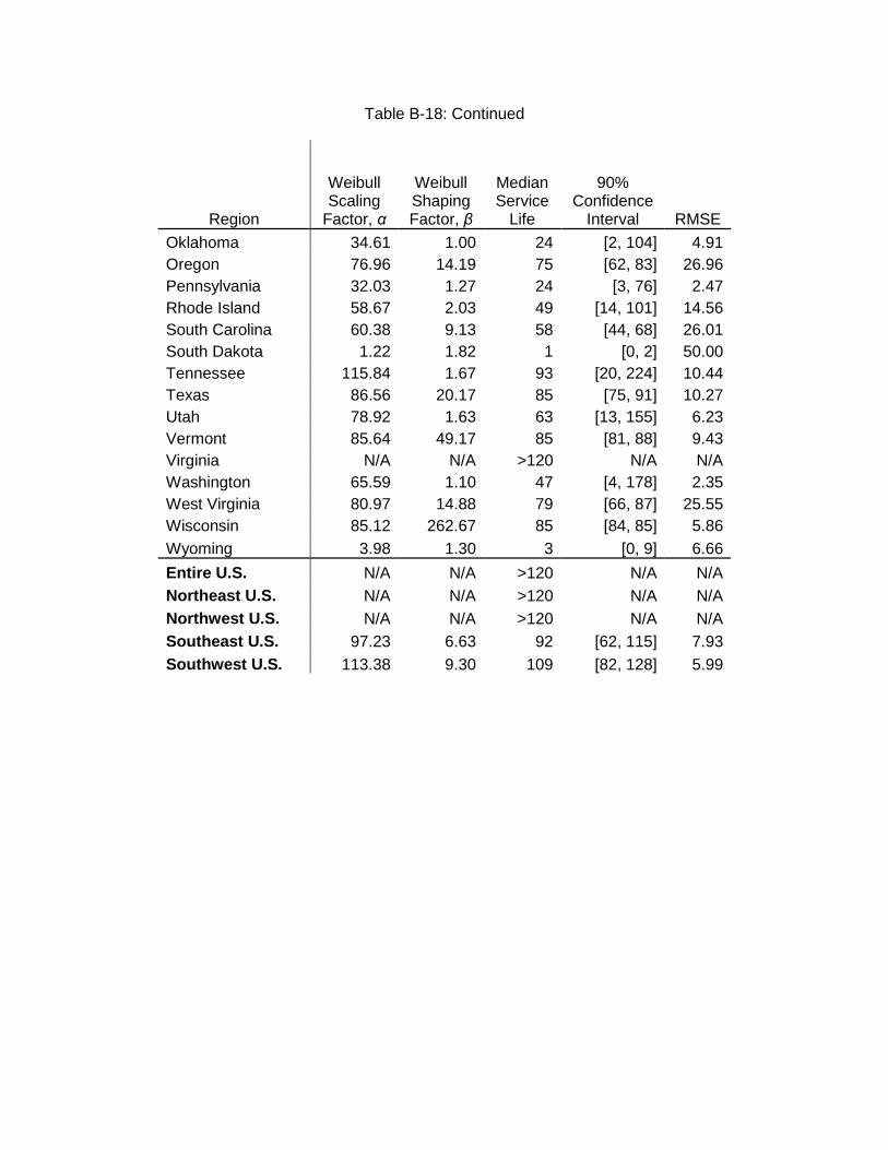
48
Table B-18: Continued
Region
Weibull Scaling
Factor, α
Weibull Shaping Factor, β
Median Service
Life
90% Confidence
Interval RMSE
Oklahoma 34.61 1.00 24 [2, 104] 4.91 Oregon 76.96 14.19 75 [62, 83] 26.96 Pennsylvania 32.03 1.27 24 [3, 76] 2.47 Rhode Island 58.67 2.03 49 [14, 101] 14.56 South Carolina 60.38 9.13 58 [44, 68] 26.01 South Dakota 1.22 1.82 1 [0, 2] 50.00 Tennessee 115.84 1.67 93 [20, 224] 10.44 Texas 86.56 20.17 85 [75, 91] 10.27 Utah 78.92 1.63 63 [13, 155] 6.23 Vermont 85.64 49.17 85 [81, 88] 9.43 Virginia N/A N/A >120 N/A N/A Washington 65.59 1.10 47 [4, 178] 2.35 West Virginia 80.97 14.88 79 [66, 87] 25.55 Wisconsin 85.12 262.67 85 [84, 85] 5.86 Wyoming 3.98 1.30 3 [0, 9] 6.66
Entire U.S. N/A N/A >120 N/A N/A Northeast U.S. N/A N/A >120 N/A N/A Northwest U.S. N/A N/A >120 N/A N/A Southeast U.S. 97.23 6.63 92 [62, 115] 7.93 Southwest U.S. 113.38 9.30 109 [82, 128] 5.99

49
Table B-19: Indiana Bridge Deck Transition Matrices
Age Group Annual Transition Probabilities
9 → 8 8 → 7 7 → 6 6 → 5 5 → 4 4 → 3 0 → 6 years 36.02 12.07 5.02 4.07 2.36 8.71 7 → 12 yrs 42.41 14.15 6.18 4.96 3.94 5.03 13 → 18 yrs 38.17 14.00 6.45 5.48 4.96 3.19 19 → 24 yrs 57.36 16.18 7.06 5.67 4.73 2.62 25 → 30 yrs 66.67 21.02 7.37 5.70 3.95 2.50 31 → 36 yrs 24.41 22.69 9.04 5.10 4.46 2.78 37 → 42 yrs 42.26 24.02 10.34 5.98 3.11 2.53 43 → 48 yrs 55.28 15.48 10.37 6.14 4.11 2.99 49 → 54 yrs 55.28 26.72 9.91 8.23 4.34 1.87 55 → 60 yrs 29.29 26.62 12.81 7.43 4.81 3.53 61 → 66 yrs 46.55 29.29 14.81 8.55 5.37 4.72 67 → 72 yrs 36.75 22.04 13.75 8.88 4.94 4.72 73 → 78 yrs 100.00 22.30 14.97 8.35 5.07 5.25 79 → 84 yrs 100.00 37.98 16.84 9.34 6.46 4.12 85 → 90 yrs N/A 22.54 13.99 10.09 5.75 4.31 91 → 96 yrs 22.54 30.99 14.37 12.02 6.96 7.05 97 → 102 yrs 0.00 22.54 17.04 10.05 8.18 5.41 103 → 108 yrs 100.00 32.58 14.72 9.86 9.86 4.88 109 → 114 yrs N/A 8.71 10.20 8.09 2.47 7.42 115 → 120 yrs N/A 5.72 21.83 5.72 7.65 0.00
Table B-20: Indiana Bridge Superstructure Transition Matrices
Age Group Annual Transition Probabilities
9 → 8 8 → 7 7 → 6 6 → 5 5 → 4 4 → 3 0 → 6 years 31.53 6.68 2.78 3.34 4.77 2.67 7 → 12 yrs 34.77 7.99 3.80 4.38 5.64 5.72 13 → 18 yrs 32.84 9.24 4.61 4.27 4.60 4.35 19 → 24 yrs 100.00 10.46 5.06 4.94 4.54 4.48 25 → 30 yrs 18.35 12.11 5.10 4.27 5.92 2.67 31 → 36 yrs 29.29 15.47 5.88 5.90 5.53 3.79 37 → 42 yrs 29.29 19.44 7.49 6.10 4.45 5.21 43 → 48 yrs 100.00 14.16 8.00 6.99 4.89 6.61 49 → 54 yrs 18.35 23.07 8.62 7.63 5.98 6.03 55 → 60 yrs 18.35 24.04 10.20 7.67 5.87 3.28 61 → 66 yrs 29.29 18.94 10.27 9.68 6.17 4.06 67 → 72 yrs 29.29 25.17 14.66 10.14 6.70 5.30 73 → 78 yrs 100.00 29.29 15.78 8.50 7.68 4.38 79 → 84 yrs N/A 18.35 12.96 8.96 7.43 5.87 85 → 90 yrs N/A 22.54 9.11 7.42 6.77 5.64 91 → 96 yrs N/A 22.54 15.48 13.21 7.76 5.85 97 → 102 yrs N/A N/A 11.65 15.73 6.65 7.50 103 → 108 yrs N/A 100.00 25.46 6.75 9.99 6.19 109 → 114 yrs N/A N/A 4.26 9.55 6.14 1.44 115 → 120 yrs N/A 0.00 50.00 1.68 4.96 7.80

50
Table B-21: Indiana Bridge Substructure Transition Matrices
Age Group Annual Transition Probabilities
9 → 8 8 → 7 7 → 6 6 → 5 5 → 4 4 → 3 0 → 6 years 31.44 5.70 2.28 3.36 3.39 1.57 7 → 12 yrs 33.10 7.57 3.41 4.41 4.64 5.42 13 → 18 yrs 24.72 8.14 4.42 4.58 4.25 3.72 19 → 24 yrs 50.00 9.88 4.84 5.18 5.53 3.45 25 → 30 yrs 29.29 11.68 4.66 5.50 4.41 3.38 31 → 36 yrs 100.00 13.77 5.18 5.61 5.39 4.61 37 → 42 yrs 29.29 14.17 6.99 5.52 5.26 4.32 43 → 48 yrs 100.00 7.34 7.20 5.70 4.18 7.01 49 → 54 yrs 100.00 17.16 7.46 6.03 4.98 3.68 55 → 60 yrs 29.29 23.62 9.30 6.55 5.89 5.26 61 → 66 yrs N/A 22.54 11.10 8.13 6.72 4.96 67 → 72 yrs N/A 35.11 12.48 8.47 7.38 5.33 73 → 78 yrs N/A 13.40 10.21 9.46 6.20 5.17 79 → 84 yrs N/A 10.56 11.81 9.24 6.06 5.25 85 → 90 yrs N/A 14.72 11.88 7.70 5.23 5.74 91 → 96 yrs N/A 22.54 13.98 10.00 6.37 8.04 97 → 102 yrs N/A 100.00 16.79 6.66 6.78 7.07 103 → 108 yrs N/A N/A 15.76 6.32 5.47 6.07 109 → 114 yrs N/A N/A 21.83 7.53 4.19 6.07 115 → 120 yrs N/A 29.29 25.46 9.42 9.55 3.18
Table B-22: Indiana Bridge Channel Protection Transition Matrices
Age Group Annual Transition Probabilities
9 → 8 8 → 7 7 → 6 6 → 5 5 → 4 4 → 3 0 → 6 years 35.31 8.27 4.30 3.18 1.82 0.43 7 → 12 yrs 13.67 10.05 5.33 3.50 3.34 1.84 13 → 18 yrs 13.60 10.16 5.33 3.48 2.80 1.57 19 → 24 yrs 29.29 11.83 6.85 3.73 2.91 1.67 25 → 30 yrs 7.42 13.72 7.70 4.69 3.17 1.47 31 → 36 yrs 13.40 13.43 8.08 5.04 2.57 1.80 37 → 42 yrs 14.72 12.58 7.91 5.41 2.92 2.17 43 → 48 yrs 29.29 6.62 8.62 5.65 3.42 3.09 49 → 54 yrs 0.00 12.47 10.00 5.96 5.00 1.42 55 → 60 yrs 29.29 22.35 10.90 7.32 5.50 2.42 61 → 66 yrs 29.29 15.79 11.25 8.30 5.52 2.87 67 → 72 yrs 13.40 23.30 11.16 8.64 5.86 2.23 73 → 78 yrs 10.56 13.40 10.43 9.41 5.21 3.35 79 → 84 yrs 18.35 10.94 11.11 7.49 5.88 3.91 85 → 90 yrs 0.00 6.75 9.59 5.75 5.01 2.45 91 → 96 yrs N/A 7.42 12.26 7.60 4.53 1.94 97 → 102 yrs 100.00 10.56 7.42 4.65 3.95 5.05 103 → 108 yrs 100.00 5.72 11.99 5.55 3.98 0.00 109 → 114 yrs N/A 0.00 4.83 5.64 3.64 0.00 115 → 120 yrs N/A 29.29 8.71 0.00 7.07 0.00
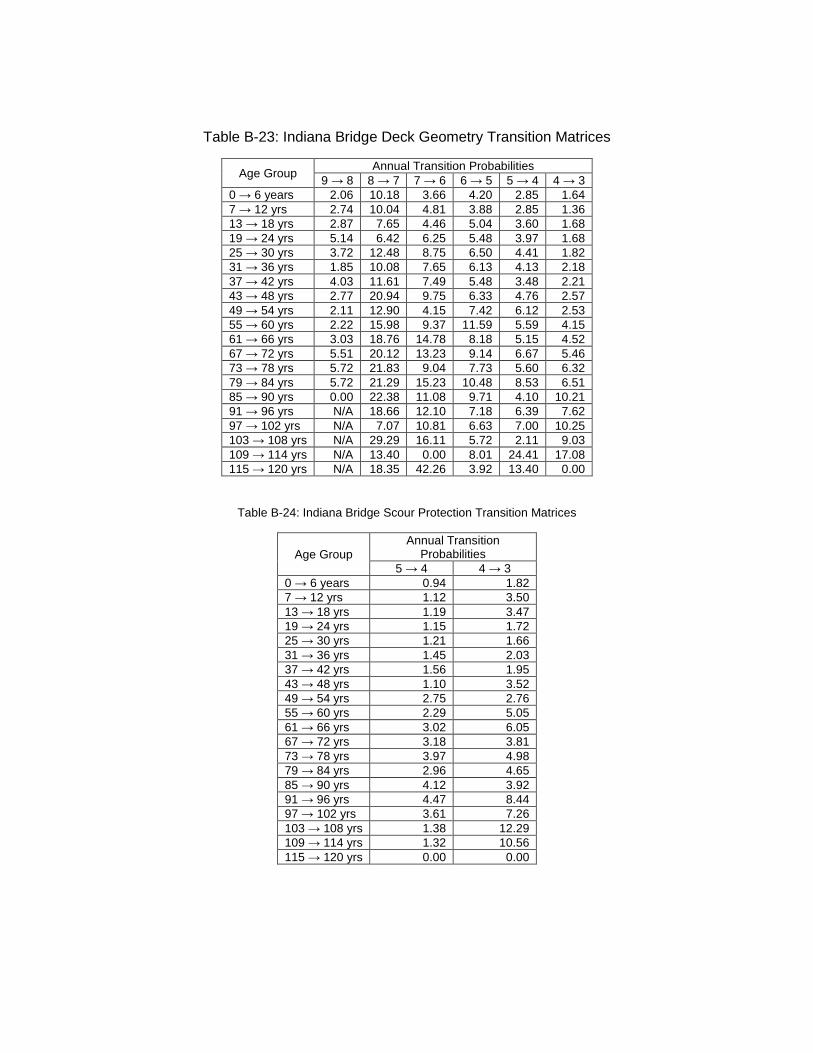
51
Table B-23: Indiana Bridge Deck Geometry Transition Matrices
Age Group Annual Transition Probabilities
9 → 8 8 → 7 7 → 6 6 → 5 5 → 4 4 → 3 0 → 6 years 2.06 10.18 3.66 4.20 2.85 1.64 7 → 12 yrs 2.74 10.04 4.81 3.88 2.85 1.36 13 → 18 yrs 2.87 7.65 4.46 5.04 3.60 1.68 19 → 24 yrs 5.14 6.42 6.25 5.48 3.97 1.68 25 → 30 yrs 3.72 12.48 8.75 6.50 4.41 1.82 31 → 36 yrs 1.85 10.08 7.65 6.13 4.13 2.18 37 → 42 yrs 4.03 11.61 7.49 5.48 3.48 2.21 43 → 48 yrs 2.77 20.94 9.75 6.33 4.76 2.57 49 → 54 yrs 2.11 12.90 4.15 7.42 6.12 2.53 55 → 60 yrs 2.22 15.98 9.37 11.59 5.59 4.15 61 → 66 yrs 3.03 18.76 14.78 8.18 5.15 4.52 67 → 72 yrs 5.51 20.12 13.23 9.14 6.67 5.46 73 → 78 yrs 5.72 21.83 9.04 7.73 5.60 6.32 79 → 84 yrs 5.72 21.29 15.23 10.48 8.53 6.51 85 → 90 yrs 0.00 22.38 11.08 9.71 4.10 10.21 91 → 96 yrs N/A 18.66 12.10 7.18 6.39 7.62 97 → 102 yrs N/A 7.07 10.81 6.63 7.00 10.25 103 → 108 yrs N/A 29.29 16.11 5.72 2.11 9.03 109 → 114 yrs N/A 13.40 0.00 8.01 24.41 17.08 115 → 120 yrs N/A 18.35 42.26 3.92 13.40 0.00
Table B-24: Indiana Bridge Scour Protection Transition Matrices
Age Group Annual Transition
Probabilities 5 → 4 4 → 3
0 → 6 years 0.94 1.82 7 → 12 yrs 1.12 3.50 13 → 18 yrs 1.19 3.47 19 → 24 yrs 1.15 1.72 25 → 30 yrs 1.21 1.66 31 → 36 yrs 1.45 2.03 37 → 42 yrs 1.56 1.95 43 → 48 yrs 1.10 3.52 49 → 54 yrs 2.75 2.76 55 → 60 yrs 2.29 5.05 61 → 66 yrs 3.02 6.05 67 → 72 yrs 3.18 3.81 73 → 78 yrs 3.97 4.98 79 → 84 yrs 2.96 4.65 85 → 90 yrs 4.12 3.92 91 → 96 yrs 4.47 8.44 97 → 102 yrs 3.61 7.26 103 → 108 yrs 1.38 12.29 109 → 114 yrs 1.32 10.56 115 → 120 yrs 0.00 0.00

52
Table B-25: Number of Observations used in Developing Indiana Bridge Deck Transition Matrices
Age Group No. of Annual and Biannual Inspection Pairs by Starting
Condition State 9 8 7 6 5 4
0 → 6 years 3,545 12,149 8,073 1,404 257 30 7 → 12 yrs 205 6,748 12,106 3,825 712 102 13 → 18 yrs 34 3,191 10,832 5,165 1,210 207 19 → 24 yrs 11 1,362 7,867 4,549 1,365 271 25 → 30 yrs 9 715 5,547 4,001 1,252 263 31 → 36 yrs 7 343 3,550 3,329 1,226 255 37 → 42 yrs 9 194 1,840 2,268 932 200 43 → 48 yrs 5 77 768 1,118 721 170 49 → 54 yrs 5 54 520 868 577 189 55 → 60 yrs 8 52 609 1,174 724 202 61 → 66 yrs 7 58 700 1,314 919 304 67 → 72 yrs 5 51 488 1,143 871 336 73 → 78 yrs 2 53 260 756 719 323 79 → 84 yrs 1 39 188 595 472 223 85 → 90 yrs 0 20 123 427 349 166 91 → 96 yrs 5 21 90 208 253 125 97 → 102 yrs 1 5 77 110 102 57 103 → 108 yrs 2 11 55 96 48 21 109 → 114 yrs 0 6 31 58 41 14 115 → 120 yrs 0 9 18 18 34 10
Table B-26: Number of Observations used in Developing Indiana Bridge Superstructure Transition Matrices
Age Group No. of Annual and Biannual Inspection Pairs by Starting
Condition State 9 8 7 6 5 4
0 → 6 years 3,679 11,436 8,240 1,506 365 76 7 → 12 yrs 322 9,306 10,957 2,486 566 180 13 → 18 yrs 51 5,963 11,125 3,240 734 223 19 → 24 yrs 6 3,328 8,411 3,085 867 217 25 → 30 yrs 3 1,938 6,347 2,848 958 266 31 → 36 yrs 2 890 4,356 2,462 967 350 37 → 42 yrs 4 282 2,482 1,758 804 286 43 → 48 yrs 1 95 1,016 949 671 219 49 → 54 yrs 3 49 564 811 603 231 55 → 60 yrs 6 26 630 1,023 833 372 61 → 66 yrs 6 35 657 1,080 1,070 566 67 → 72 yrs 4 25 427 930 1,027 649 73 → 78 yrs 1 10 203 645 785 537 79 → 84 yrs 0 3 99 450 552 430 85 → 90 yrs 0 5 69 273 382 283 91 → 96 yrs 0 10 42 150 248 185 97 → 102 yrs 0 0 41 69 140 90 103 → 108 yrs 0 1 27 69 79 50 109 → 114 yrs 0 0 12 55 42 35 115 → 120 yrs 0 1 4 30 31 20

53
Table B-27: Number of Observations used in Developing Indiana Bridge Substructure Transition Matrices
Age Group No. of Annual and Biannual Inspection Pairs by Starting
Condition State 9 8 7 6 5 4
0 → 6 years 3,342 10,897 8,979 1,679 420 96 7 → 12 yrs 286 8,942 10,927 2,831 817 218 13 → 18 yrs 30 5,294 10,614 3,856 1,251 329 19 → 24 yrs 8 2,743 7,732 3,558 1,450 443 25 → 30 yrs 6 1,650 5,626 3,093 1,346 467 31 → 36 yrs 1 854 4,013 2,395 1,191 477 37 → 42 yrs 2 319 2,268 1,787 859 343 43 → 48 yrs 1 99 944 1,020 648 207 49 → 54 yrs 1 51 564 787 566 263 55 → 60 yrs 2 60 581 1,058 708 420 61 → 66 yrs 0 35 596 1,173 963 558 67 → 72 yrs 0 19 440 937 922 646 73 → 78 yrs 0 8 222 616 732 536 79 → 84 yrs 0 10 144 414 604 391 85 → 90 yrs 0 11 94 297 432 242 91 → 96 yrs 0 5 50 200 292 162 97 → 102 yrs 0 1 39 101 145 88 103 → 108 yrs 0 0 31 98 94 34 109 → 114 yrs 0 0 18 69 61 17 115 → 120 yrs 0 2 9 39 22 16
Table B-28: Number of Observations used in Developing Indiana Bridge Channel Protection Transition Matrices
Age Group No. of Annual and Biannual Inspection Pairs by Starting
Condition State 9 8 7 6 5 4
0 → 6 years 1,257 8,409 6,795 2,521 667 116 7 → 12 yrs 161 5,205 8,247 4,032 1,051 274 13 → 18 yrs 71 2,985 7,871 4,817 1,447 384 19 → 24 yrs 36 1,491 5,831 4,663 1,656 514 25 → 30 yrs 14 798 4,073 4,018 1,745 550 31 → 36 yrs 16 455 2,593 3,000 1,598 504 37 → 42 yrs 11 263 1,428 1,911 1,114 350 43 → 48 yrs 4 125 697 1,065 700 230 49 → 54 yrs 1 77 500 813 554 249 55 → 60 yrs 4 68 660 971 682 419 61 → 66 yrs 2 55 692 1,157 904 547 67 → 72 yrs 4 51 536 980 888 567 73 → 78 yrs 5 20 349 669 670 516 79 → 84 yrs 3 29 243 527 464 326 85 → 90 yrs 2 23 208 340 307 248 91 → 96 yrs 0 21 126 253 226 130 97 → 102 yrs 1 10 91 121 142 61 103 → 108 yrs 1 9 71 102 77 21 109 → 114 yrs 0 4 53 73 42 11 115 → 120 yrs 0 2 30 40 22 11

54
Table B-29: Number of Observations used in Developing Indiana Bridge Deck Geometry Transition Matrices
Age Group No. of Annual and Biannual Inspection Pairs by Starting
Condition State 9 8 7 6 5 4
0 → 6 years 2,989 238 3,354 6,501 6,880 3,840 7 → 12 yrs 2,052 278 2,835 5,854 6,702 4,548 13 → 18 yrs 1,167 265 2,075 4,940 6,542 4,515 19 → 24 yrs 539 193 1,197 3,461 5,610 3,783 25 → 30 yrs 274 94 478 2,346 4,750 3,359 31 → 36 yrs 109 47 204 1,321 3,400 2,947 37 → 42 yrs 76 32 111 563 1,990 2,034 43 → 48 yrs 110 32 97 269 839 1,065 49 → 54 yrs 96 29 123 189 514 721 55 → 60 yrs 91 51 168 229 571 910 61 → 66 yrs 67 100 168 204 568 1,031 67 → 72 yrs 28 105 170 172 434 809 73 → 78 yrs 18 108 139 148 248 474 79 → 84 yrs 9 92 167 141 153 238 85 → 90 yrs 2 83 129 92 137 129 91 → 96 yrs 0 65 88 65 97 75 97 → 102 yrs 0 22 44 39 37 36 103 → 108 yrs 0 12 27 27 24 29 109 → 114 yrs 0 4 11 26 7 16 115 → 120 yrs 0 3 3 13 4 8
Table B-30: Number of Observations used in Developing Indiana Bridge Scour Protection Transition Matrices
Age Group
No. of Annual and Biannual Inspection Pairs by Starting
Condition State 5 4 3
0 → 6 years 2,659 166 85 7 → 12 yrs 3,275 305 151 13 → 18 yrs 3,459 352 200 19 → 24 yrs 3,150 468 153 25 → 30 yrs 2,869 486 179 31 → 36 yrs 2,325 399 162 37 → 42 yrs 1,582 336 119 43 → 48 yrs 959 159 45 49 → 54 yrs 534 92 56 55 → 60 yrs 442 122 89 61 → 66 yrs 572 162 150 67 → 72 yrs 608 241 173 73 → 78 yrs 501 206 167 79 → 84 yrs 360 110 121 85 → 90 yrs 310 78 74 91 → 96 yrs 206 68 51 97 → 102 yrs 127 50 45 103 → 108 yrs 73 13 30 109 → 114 yrs 38 5 30 115 → 120 yrs 18 1 8

55
Appendix C. Box Culvert Markov/Weibull Results by State and ‘Failure Mechanism’
Table C-1: Box Culvert Condition Markov/Weibull Results (End-of-Life Threshold: Culvert Condition Rating = 3)
Region
Weibull Scaling
Factor, α
Weibull Shape
Factor, β
Median Service
Life
90% Confidence
Interval RMSE
Alabama 113.79 10.83 110 [86, 126] 8.07 Alaska 51.41 13.17 50 [41, 56] 11.71 Arizona 73.58 5.70 69 [44, 89] 8.05 Arkansas 87.33 97.35 87 [85, 88] 5.16 California 99.39 93.99 99 [96, 101] 6.11 Colorado 99.31 15.59 97 [82, 107] 10.88 Connecticut 84.23 7.12 80 [55, 98] 7.06 Delaware 57.30 2.34 49 [16, 92] 8.17 Florida 90.46 7.25 86 [60, 105] 6.19 Georgia 107.21 12.06 104 [84, 117] 7.47 Hawaii 72.75 6.93 69 [47, 85] 9.69 Idaho 104.79 5.47 98 [61, 128] 9.31 Illinois 117.79 4.72 109 [63, 149] 8.88 Indiana 104.57 4.88 97 [57, 131] 7.27 Iowa 118.30 4.48 109 [61, 151] 8.60 Kansas 117.16 5.82 110 [70, 141] 7.86 Kentucky 104.39 4.99 97 [58, 130] 9.86 Louisiana 87.35 90.43 87 [85, 88] 6.08 Maine 57.65 2.26 49 [15, 94] 4.60 Maryland 86.43 4.08 79 [42, 113] 9.61 Massachusetts 85.78 4.45 79 [44, 110] 14.87 Michigan 67.92 3.41 61 [28, 94] 5.64 Minnesota 97.09 3.34 87 [40, 135] 2.15 Mississippi 100.31 117.73 100 [98, 101] 5.25 Missouri 109.21 190.11 109 [108, 110] 4.75 Montana 76.89 9.56 74 [56, 86] 14.63 Nebraska 105.14 268.16 105 [104, 106] 6.17 Nevada 70.83 6.59 67 [45, 84] 13.96 New Hampshire 119.30 2.49 103 [36, 185] 6.90 New Jersey 108.26 7.36 103 [72, 126] 8.25

56
Table C-1: Continued
Region
Weibull Scaling
Factor, α
Weibull Shape
Factor, β
Median Service
Life
90% Confidence
Interval RMSE
New Mexico 84.18 7.20 80 [56, 98] 8.39 New York 81.70 2.17 69 [21, 135] 4.92 North Carolina 107.09 9.40 103 [78, 120] 7.82 North Dakota 85.09 344.13 85 [84, 85] 6.20 Ohio 69.93 3.04 62 [26, 100] 4.09 Oklahoma 87.48 3.60 79 [38, 119] 5.79 Oregon 74.02 4.32 68 [37, 95] 11.33 Pennsylvania 110.24 5.40 103 [64, 135] 6.37 Rhode Island 20.72 4.23 19 [10, 27] 17.65 South Dakota 84.24 4.77 78 [45, 106] 3.89 Tennessee 114.08 13.41 111 [91, 124] 6.09 Texas 110.64 5.12 103 [62, 137] 5.57 Utah 76.00 13.75 74 [61, 82] 10.36 Vermont 105.42 2.49 91 [32, 164] 15.03 Virginia 79.34 85.81 79 [77, 80] 5.12 Washington 73.09 6.36 69 [46, 87] 5.09 West Virginia 92.38 89.92 92 [89, 94] 6.33 Wisconsin 113.41 2.35 97 [32, 181] 8.74 Wyoming 79.42 69.62 79 [76, 81] 9.44
Entire U.S. 112.35 4.22 103 [56, 146] 1.81 Northeast U.S. 103.33 3.48 93 [44, 142] 1.99 Northwest U.S. 118.44 4.96 110 [65, 148] 7.46 Southeast U.S. 110.54 7.13 105 [73, 129] 7.14 Southwest U.S. 108.62 6.90 103 [71, 127] 6.84

57
Table C-31: Box Culvert Condition Markov/Weibull Results (End-of-Life Threshold: Culvert Condition Rating = 4)
Region
Weibull Scaling
Factor, α
Weibull Shape
Factor, β
Median Service
Life
90% Confidence
Interval RMSE
Alabama 116.98 5.19 109 [66, 145] 10.71 Alaska 50.57 11.59 49 [39, 56] 11.76 Arizona 72.59 5.61 68 [43, 88] 8.11 Arkansas 86.33 96.16 86 [84, 87] 6.50 California 98.42 85.69 98 [95, 100] 7.64 Colorado 95.33 3.56 86 [41, 130] 9.39 Connecticut 85.73 4.48 79 [44, 110] 6.36 Delaware 50.76 2.21 43 [13, 83] 9.84 Florida 90.99 5.38 85 [52, 112] 7.36 Georgia 121.06 2.27 103 [33, 196] 6.59 Hawaii 71.78 6.77 68 [46, 84] 9.77 Idaho 104.83 4.72 97 [56, 132] 9.78 Illinois 116.62 3.20 104 [46, 164] 7.93 Indiana 83.51 3.41 75 [35, 115] 5.03 Iowa 85.70 3.89 78 [40, 114] 2.20 Kansas 121.30 3.43 109 [51, 167] 6.68 Kentucky 93.47 3.86 85 [43, 124] 8.41 Louisiana 86.35 89.34 86 [84, 87] 6.11 Maine 43.51 1.93 36 [9, 77] 7.46 Maryland 74.46 2.70 65 [25, 112] 5.15 Massachusetts 81.74 3.68 74 [36, 110] 13.77 Michigan 63.35 2.97 56 [23, 92] 4.22 Minnesota 71.22 2.99 63 [26, 103] 1.84 Mississippi 99.31 116.69 99 [97, 100] 5.10 Missouri 97.15 5.61 91 [57, 118] 4.26 Montana 75.89 9.44 73 [55, 85] 14.89 Nebraska 104.14 265.30 104 [103, 105] 5.60 Nevada 57.36 8.72 55 [41, 65] 19.35 New Hampshire 111.23 2.18 94 [28, 184] 6.10 New Jersey 97.24 5.52 91 [57, 119] 5.72 New Mexico 92.15 2.38 79 [26, 146] 7.82 New York 53.00 1.97 44 [12, 93] 3.60 North Carolina 99.64 5.31 93 [57, 122] 6.71 North Dakota 80.35 84.18 80 [78, 81] 4.51 Ohio 48.59 2.52 42 [15, 75] 3.64

58
Table C-31: Continued
Region
Weibull Scaling
Factor, α
Weibull Shape
Factor, β
Median Service
Life
90% Confidence
Interval RMSE
Oklahoma 64.95 2.81 57 [23, 96] 1.81 Oregon 71.93 5.16 67 [40, 89] 10.45 Pennsylvania 90.47 2.70 79 [30, 136] 3.74 Rhode Island 17.65 3.73 16 [8, 24] 16.68 South Dakota 66.72 4.09 61 [32, 87] 3.13 Tennessee 113.41 11.99 110 [89, 124] 6.58 Texas 88.12 6.12 83 [54, 105] 7.88 Utah 76.49 7.86 73 [52, 88] 6.87 Vermont 88.85 3.49 80 [38, 122] 15.25 Virginia 88.66 2.60 77 [28, 135] 13.49 Washington 72.23 6.08 68 [44, 87] 5.65 West Virginia 93.21 15.24 91 [77, 100] 9.68 Wisconsin 73.57 3.37 66 [31, 102] 5.02 Wyoming 80.16 3.92 73 [38, 106] 11.24
Entire U.S. 93.69 3.77 85 [43, 125] 3.68 Northeast U.S. 83.27 3.10 74 [32, 119] 3.29 Northwest U.S. 124.61 2.74 109 [42, 186] 7.50 Southeast U.S. 116.11 3.33 104 [48, 161] 6.10 Southwest U.S. 112.04 2.54 97 [35, 173] 8.31
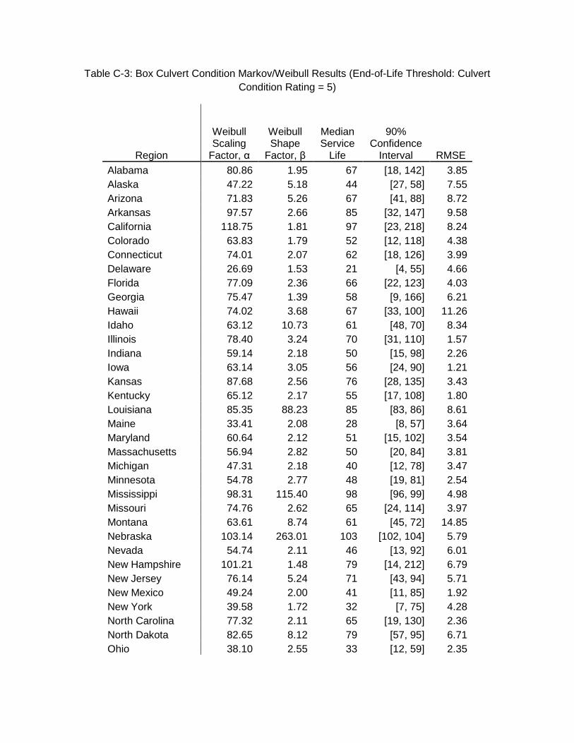
59
Table C-3: Box Culvert Condition Markov/Weibull Results (End-of-Life Threshold: Culvert Condition Rating = 5)
Region
Weibull Scaling
Factor, α
Weibull Shape
Factor, β
Median Service
Life
90% Confidence
Interval RMSE
Alabama 80.86 1.95 67 [18, 142] 3.85 Alaska 47.22 5.18 44 [27, 58] 7.55 Arizona 71.83 5.26 67 [41, 88] 8.72 Arkansas 97.57 2.66 85 [32, 147] 9.58 California 118.75 1.81 97 [23, 218] 8.24 Colorado 63.83 1.79 52 [12, 118] 4.38 Connecticut 74.01 2.07 62 [18, 126] 3.99 Delaware 26.69 1.53 21 [4, 55] 4.66 Florida 77.09 2.36 66 [22, 123] 4.03 Georgia 75.47 1.39 58 [9, 166] 6.21 Hawaii 74.02 3.68 67 [33, 100] 11.26 Idaho 63.12 10.73 61 [48, 70] 8.34 Illinois 78.40 3.24 70 [31, 110] 1.57 Indiana 59.14 2.18 50 [15, 98] 2.26 Iowa 63.14 3.05 56 [24, 90] 1.21 Kansas 87.68 2.56 76 [28, 135] 3.43 Kentucky 65.12 2.17 55 [17, 108] 1.80 Louisiana 85.35 88.23 85 [83, 86] 8.61 Maine 33.41 2.08 28 [8, 57] 3.64 Maryland 60.64 2.12 51 [15, 102] 3.54 Massachusetts 56.94 2.82 50 [20, 84] 3.81 Michigan 47.31 2.18 40 [12, 78] 3.47 Minnesota 54.78 2.77 48 [19, 81] 2.54 Mississippi 98.31 115.40 98 [96, 99] 4.98 Missouri 74.76 2.62 65 [24, 114] 3.97 Montana 63.61 8.74 61 [45, 72] 14.85 Nebraska 103.14 263.01 103 [102, 104] 5.79 Nevada 54.74 2.11 46 [13, 92] 6.01 New Hampshire 101.21 1.48 79 [14, 212] 6.79 New Jersey 76.14 5.24 71 [43, 94] 5.71 New Mexico 49.24 2.00 41 [11, 85] 1.92 New York 39.58 1.72 32 [7, 75] 4.28 North Carolina 77.32 2.11 65 [19, 130] 2.36 North Dakota 82.65 8.12 79 [57, 95] 6.71 Ohio 38.10 2.55 33 [12, 59] 2.35

60
Table C-3: Continued
Region
Weibull Scaling
Factor, α
Weibull Shape
Factor, β
Median Service
Life
90% Confidence
Interval RMSE
Oklahoma 44.57 1.97 37 [10, 78] 1.96 Oregon 68.33 2.50 59 [21, 106] 8.33 Pennsylvania 60.44 2.16 51 [15, 100] 1.85 Rhode Island 20.89 1.11 15 [1, 56] 7.54 South Dakota 51.79 3.09 46 [20, 74] 0.99 Tennessee 126.44 2.47 109 [38, 197] 5.27 Texas 64.43 2.32 55 [18, 103] 3.09 Utah 79.76 3.15 71 [31, 113] 4.58 Vermont 37.14 2.46 32 [11, 58] 4.56 Virginia 54.09 1.78 44 [10, 100] 4.75 Washington 75.52 3.06 67 [29, 108] 11.93 West Virginia 80.01 2.74 70 [27, 119] 6.27 Wisconsin 60.96 2.62 53 [20, 93] 1.15 Wyoming 61.10 5.28 57 [35, 75] 8.40
Entire U.S. 70.62 2.50 61 [22, 109] 1.19 Northeast U.S. 60.61 2.39 52 [18, 96] 1.14 Northwest U.S. 87.03 2.71 76 [29, 131] 2.66 Southeast U.S. 87.35 2.21 74 [23, 144] 2.86 Southwest U.S. 65.25 2.14 55 [16, 109] 1.81

61
Table C-4: Box Culvert Channel/Embankment Protection Markov/Weibull Results (End-of-Life Threshold: Channel Condition Rating = 3)
Region
Weibull Scaling
Factor, α
Weibull Shape
Factor, β
Median Service
Life
90% Confidence
Interval RMSE
Alabama 116.46 6.42 110 [73, 138] 8.22 Alaska 59.69 7.94 57 [41, 69] 10.13 Arizona 69.21 123.49 69 [68, 70] 8.03 Arkansas 89.26 9.85 86 [66, 100] 8.81 California 101.67 55.83 101 [96, 104] 8.16 Colorado 100.34 15.52 98 [83, 108] 11.45 Connecticut 73.69 39.05 73 [68, 76] 8.08 Delaware 79.34 4.40 73 [40, 102] 12.10 Florida 106.25 4.53 98 [55, 135] 8.90 Georgia 102.41 15.39 100 [84, 110] 6.27 Hawaii 74.62 44.21 74 [70, 76] 9.30 Idaho 76.96 14.19 75 [62, 83] 16.05 Illinois 110.46 88.08 110 [107, 112] 5.88 Indiana 103.22 8.79 99 [74, 117] 8.57 Iowa 109.57 70.71 109 [105, 111] 7.20 Kansas 119.43 4.45 110 [61, 153] 8.78 Kentucky 90.56 5.79 85 [54, 109] 7.19 Louisiana 88.50 12.79 86 [70, 96] 5.46 Maine 71.22 4.01 65 [34, 94] 5.71 Maryland 118.46 4.95 110 [65, 148] 8.99 Massachusetts 64.51 9.25 62 [47, 73] 14.19 Michigan 93.21 15.24 91 [77, 100] 12.41 Minnesota 97.24 6.62 92 [62, 115] 2.82 Mississippi 100.60 61.13 100 [96, 102] 6.07 Missouri 109.06 630.24 109 [109, 109] 1.76 Montana 79.33 8.56 76 [56, 90] 11.92 Nebraska 108.55 25.49 107 [97, 113] 7.06 Nevada 53.96 3.13 48 [21, 77] 11.60 New Hampshire 86.20 160.16 86 [85, 87] 6.44 New Jersey 83.10 14.35 81 [68, 90] 8.89 New Mexico 82.64 11.29 80 [64, 91] 9.31 New York 63.96 2.76 56 [22, 95] 6.85 North Carolina 88.23 14.34 86 [72, 95] 8.01 North Dakota 88.37 23.52 87 [78, 93] 7.26 Ohio 76.93 3.88 70 [36, 102] 11.48

62
Table C-4: Continued
Region
Weibull Scaling
Factor, α
Weibull Shape
Factor, β
Median Service
Life
90% Confidence
Interval RMSE
Oklahoma 98.28 28.03 97 [88, 102] 6.58 Oregon 86.14 233.30 86 [85, 87] 6.73 Pennsylvania 110.26 5.38 103 [64, 135] 15.11 Rhode Island 16.55 3.73 15 [7, 22] 27.30 South Dakota 94.52 13.58 92 [76, 102] 7.58 Tennessee 109.56 72.02 109 [105, 111] 6.35 Texas 92.48 22.67 91 [81, 97] 10.58 Utah 84.24 9.34 81 [61, 95] 8.93 Vermont 43.33 48.57 43 [41, 44] 5.59 Virginia 80.46 64.42 80 [77, 82] 8.25 Washington 75.40 69.50 75 [72, 77] 8.19 West Virginia 101.00 12.17 98 [79, 111] 7.24 Wisconsin 81.92 10.08 79 [61, 91] 11.50 Wyoming 86.09 332.46 86 [85, 86] 6.49
Entire U.S. 122.95 5.48 115 [72, 150] 4.34 Northeast U.S. 131.17 2.79 115 [45, 194] 10.17 Northwest U.S. 110.37 109.97 110 [107, 111] 6.50 Southeast U.S. N/A N/A >120 N/A N/A Southwest U.S. 100.71 13.44 98 [81, 109] 7.90
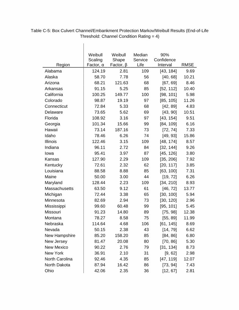
63
Table C-5: Box Culvert Channel/Embankment Protection Markov/Weibull Results (End-of-Life Threshold: Channel Condition Rating = 4)
Region
Weibull Scaling
Factor, α
Weibull Shape
Factor, β
Median Service
Life
90% Confidence
Interval RMSE
Alabama 124.19 2.81 109 [43, 184] 9.69 Alaska 58.70 7.78 56 [40, 68] 10.21 Arizona 68.21 121.63 68 [67, 69] 8.46 Arkansas 91.15 5.25 85 [52, 112] 10.40 California 100.25 149.77 100 [98, 101] 5.98 Colorado 98.87 19.19 97 [85, 105] 11.26 Connecticut 72.84 5.33 68 [42, 89] 4.83 Delaware 73.65 5.62 69 [43, 90] 10.51 Florida 108.92 3.16 97 [43, 154] 9.51 Georgia 101.34 15.66 99 [84, 109] 6.16 Hawaii 73.14 187.16 73 [72, 74] 7.33 Idaho 78.46 6.26 74 [49, 93] 15.86 Illinois 122.46 3.15 109 [48, 174] 8.57 Indiana 96.11 2.72 84 [32, 144] 9.26 Iowa 95.41 3.97 87 [45, 126] 3.80 Kansas 127.90 2.29 109 [35, 206] 7.92 Kentucky 72.61 2.32 62 [20, 117] 3.85 Louisiana 88.58 8.88 85 [63, 100] 7.31 Maine 50.00 3.00 44 [19, 72] 6.26 Maryland 128.44 2.23 109 [34, 210] 8.93 Massachusetts 63.50 9.12 61 [46, 72] 13.77 Michigan 72.44 3.38 65 [30, 100] 5.94 Minnesota 82.69 2.94 73 [30, 120] 2.96 Mississippi 99.60 60.48 99 [95, 101] 5.45 Missouri 91.23 14.80 89 [75, 98] 12.38 Montana 78.27 8.58 75 [55, 89] 11.99 Nebraska 114.64 4.68 106 [61, 145] 8.69 Nevada 50.15 2.38 43 [14, 79] 6.62 New Hampshire 85.20 158.20 85 [84, 86] 6.80 New Jersey 81.47 20.08 80 [70, 86] 5.30 New Mexico 90.22 2.76 79 [31, 134] 8.73 New York 36.91 2.10 31 [9, 62] 2.98 North Carolina 92.46 4.35 85 [47, 119] 12.07 North Dakota 87.94 16.42 86 [73, 94] 7.43 Ohio 42.06 2.35 36 [12, 67] 2.81

64
Table C-5: Continued
Region
Weibull Scaling
Factor, α
Weibull Shape
Factor, β
Median Service
Life
90% Confidence
Interval RMSE
Oklahoma 99.39 4.15 91 [49, 129] 7.57 Oregon 85.14 230.62 85 [84, 86] 6.69 Pennsylvania 56.30 2.30 48 [15, 91] 1.39 Rhode Island 15.44 3.73 14 [7, 21] 26.74 South Dakota 93.86 11.86 91 [73, 103] 8.41 Tennessee 101.08 8.89 97 [72, 114] 8.75 Texas 81.96 2.83 72 [29, 121] 8.88 Utah 83.27 9.14 80 [60, 94] 8.98 Vermont 43.47 6.26 41 [27, 52] 7.47 Virginia 89.50 2.94 79 [33, 130] 14.55 Washington 74.59 45.89 74 [70, 76] 8.54 West Virginia 110.77 2.76 97 [38, 165] 8.36 Wisconsin 67.30 3.73 61 [30, 90] 5.87 Wyoming 85.09 328.76 85 [84, 85] 5.69
Entire U.S. 102.40 2.42 88 [30, 161] 3.20 Northeast U.S. 81.83 2.58 71 [26, 125] 2.75 Northwest U.S. 119.08 4.14 109 [58, 155] 9.41 Southeast U.S. N/A N/A >120 N/A N/A Southwest U.S. 115.35 2.12 97 [28, 194] 12.35
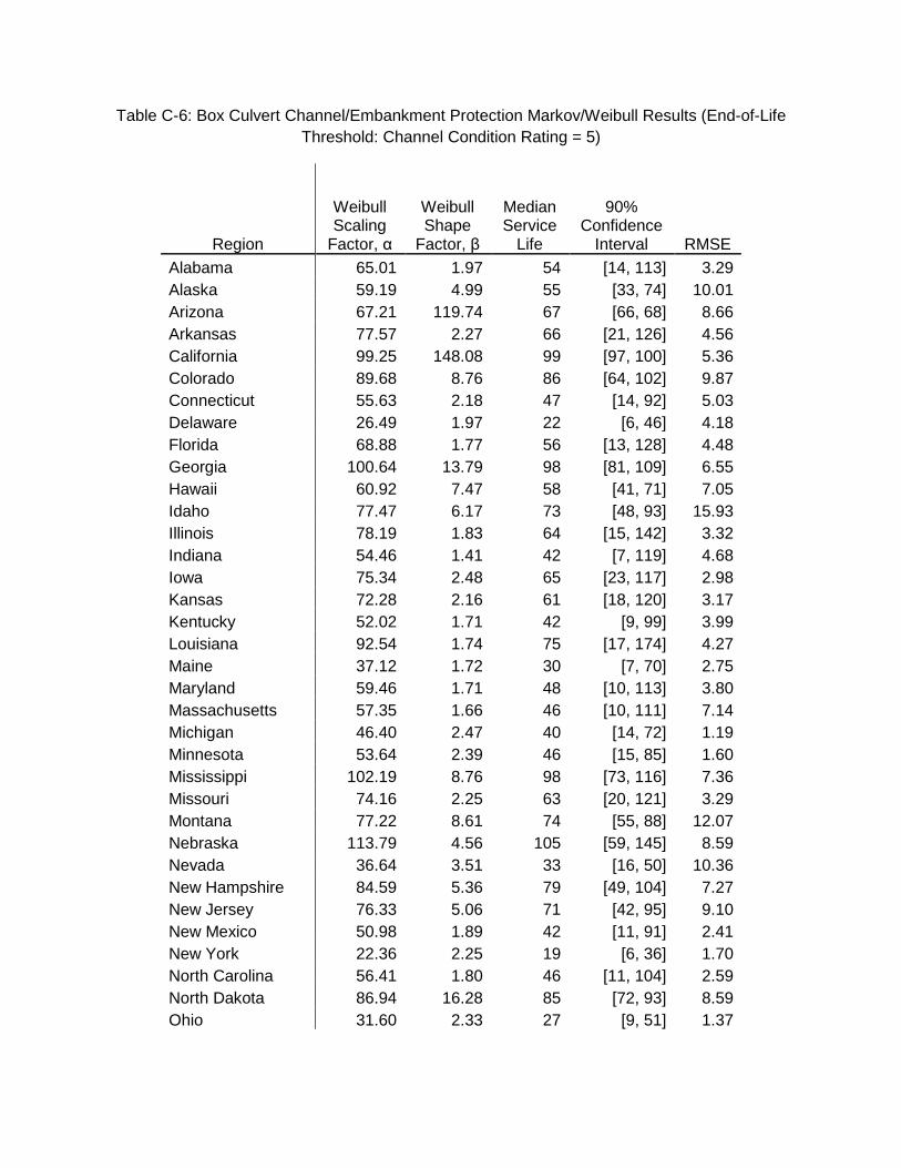
65
Table C-6: Box Culvert Channel/Embankment Protection Markov/Weibull Results (End-of-Life Threshold: Channel Condition Rating = 5)
Region
Weibull Scaling
Factor, α
Weibull Shape
Factor, β
Median Service
Life
90% Confidence
Interval RMSE
Alabama 65.01 1.97 54 [14, 113] 3.29 Alaska 59.19 4.99 55 [33, 74] 10.01 Arizona 67.21 119.74 67 [66, 68] 8.66 Arkansas 77.57 2.27 66 [21, 126] 4.56 California 99.25 148.08 99 [97, 100] 5.36 Colorado 89.68 8.76 86 [64, 102] 9.87 Connecticut 55.63 2.18 47 [14, 92] 5.03 Delaware 26.49 1.97 22 [6, 46] 4.18 Florida 68.88 1.77 56 [13, 128] 4.48 Georgia 100.64 13.79 98 [81, 109] 6.55 Hawaii 60.92 7.47 58 [41, 71] 7.05 Idaho 77.47 6.17 73 [48, 93] 15.93 Illinois 78.19 1.83 64 [15, 142] 3.32 Indiana 54.46 1.41 42 [7, 119] 4.68 Iowa 75.34 2.48 65 [23, 117] 2.98 Kansas 72.28 2.16 61 [18, 120] 3.17 Kentucky 52.02 1.71 42 [9, 99] 3.99 Louisiana 92.54 1.74 75 [17, 174] 4.27 Maine 37.12 1.72 30 [7, 70] 2.75 Maryland 59.46 1.71 48 [10, 113] 3.80 Massachusetts 57.35 1.66 46 [10, 111] 7.14 Michigan 46.40 2.47 40 [14, 72] 1.19 Minnesota 53.64 2.39 46 [15, 85] 1.60 Mississippi 102.19 8.76 98 [73, 116] 7.36 Missouri 74.16 2.25 63 [20, 121] 3.29 Montana 77.22 8.61 74 [55, 88] 12.07 Nebraska 113.79 4.56 105 [59, 145] 8.59 Nevada 36.64 3.51 33 [16, 50] 10.36 New Hampshire 84.59 5.36 79 [49, 104] 7.27 New Jersey 76.33 5.06 71 [42, 95] 9.10 New Mexico 50.98 1.89 42 [11, 91] 2.41 New York 22.36 2.25 19 [6, 36] 1.70 North Carolina 56.41 1.80 46 [11, 104] 2.59 North Dakota 86.94 16.28 85 [72, 93] 8.59 Ohio 31.60 2.33 27 [9, 51] 1.37

66
Table C-6: Continued
Region
Weibull Scaling
Factor, α
Weibull Shape
Factor, β
Median Service
Life
90% Confidence
Interval RMSE
Oklahoma 77.12 2.14 65 [19, 129] 3.39 Oregon 55.41 2.98 49 [20, 80] 4.92 Pennsylvania 32.32 2.04 27 [8, 55] 1.95 Rhode Island 14.42 3.54 13 [6, 20] 27.00 South Dakota 84.21 2.34 72 [24, 135] 7.66 Tennessee 89.86 1.89 74 [19, 161] 3.26 Texas 42.07 1.72 34 [7, 80] 1.81 Utah 84.21 5.73 79 [50, 102] 9.71 Vermont 31.88 2.82 28 [11, 47] 1.35 Virginia 39.44 1.75 32 [7, 74] 3.16 Washington 73.05 549.84 73 [73, 73] 5.26 West Virginia 69.41 1.71 56 [12, 132] 4.25 Wisconsin 48.49 2.18 41 [12, 80] 1.39 Wyoming 77.83 5.72 73 [46, 94] 8.62
Entire U.S. 66.28 1.96 55 [15, 116] 1.54 Northeast U.S. 50.95 1.90 42 [11, 91] 2.36 Northwest U.S. 85.19 2.60 74 [27, 130] 4.10 Southeast U.S. 87.99 2.12 74 [22, 148] 3.59 Southwest U.S. 56.64 1.59 45 [9, 113] 2.88

67
Appendix D. Interest Formulae for LCCA
Table D-1: Interest Formulae for LCCA (Sinha & Labi, 2007)
Note: N represents the analysis period
Description Cash Flow Diagram Computational Formula
Factor Computation1
Finding the future compounded amount (F) at the end of a specified analysis period, given the initial amount (P) and interest rate.
P F?
0 1 … … N
F = P * SPCAF
The Single Payment Compound Amount Factor, SPCAF (i%, N) may be read off from standard economic analysis tables, or may be computed as shown.
NiSPCAF )1( +=
iNeSPCAF *=
Finding the initial amount (P) that would yield a given future amount (F) at the end of a specified analysis period, given the interest rate.
P? F
0 1 … … N
P = F * SPPWF
The Single Payment Present Worth Factor, SPPWF (i%, N) may be read off from standard economic analysis tables, or may be computed as shown.
NiSPPWF
)1(
1
+=
iNeSPPWF
*
1=
Finding the uniform yearly amount (A) that would yield a given future amount (F) at the end of a specified analysis period, given the interest rate.
A? F
0 1 2 … N
A = F * SFDF
The Sinking Fund Deposit Factor, SFDF (i%, N) may be read off standard economic analysis tables, or may be computed as shown.
(1 ) 1N
iSFDF
i=
+ −
*
1
1
i
N i
eSFDF
e
−=−

68
Table D-1: Continued
Description Cash Flow Diagram Computational Formula
Factor Computation1
Finding the future compounded amount (F) at the end of a specified analysis period due to annual payments (A), given the interest rate.
A F?
0 1 2 … N
F = A * USCAF
The Uniform Series Compounded Amount Factor, USCAF (i%, N) may be read off from standard economic analysis tables, or may be computed as shown.
i
iUSCAF
N 1)1( −+=
1
1*
−−=
i
iN
e
eUSCAF
Finding the initial amount (P) that is equivalent to a series of uniform annual payments (A), given the interest rate and a specified analysis period.
P? A
0 1 2 … N
P = A * USPWF
The Uniform Series Present Worth Factor, USPWF (i%, N) may be read off from standard economic analysis tables, or may be computed as shown.
N
N
ii
iUSPWF
)1(*
1)1(
+−+=
1
1 *
−−=
−
i
iN
e
eUSPWF
Finding the amount of uniform yearly payments (A) that would completely recover an initial amount (P) at the end of a specified analysis period, given the interest rate.
P A?
0 1 2 … N
A = P * USCRF
The Uniform Series capital Recovery Factor, USCRF (i%, N) may be read off from standard economic analysis tables, or may be computed as shown.
1)1(
)1(*
−++=
N
N
i
iiUSCRF
iN
i
e
eUSCRF
*1
1−−−=
Note: 1) In column 4, upper and lower formulae are for discrete and continuous compounding, respectively. 2) For fixed discrete compounding yearly, i = nominal interest rate and N represents years. 3) When there is more than one compounding period per year, the formulae and tables can be used as long as there is a cash flow at the end of each interest period. i represents the interest rate per period and N is the number of periods. 4) When the compounding is more frequent than a year, but the cash flows are annual, the formulae can be used with N as number of years and i as the effective annual interest rate.