estimating highway subsidence due to longwall...
TRANSCRIPT

i
ESTIMATING HIGHWAY SUBSIDENCE DUE TO LONGWALL MINING
by
Juan José Gutiérrez Puertas
Ingeniero Civil, Universidad de los Andes, 2003
Master of Science, University of Pittsburgh, 2008
Submitted to the Graduate Faculty of
Swanson School of Engineering in partial fulfillment
of the requirements for the degree of
Doctor of Philosophy
University of Pittsburgh
2010

ii
UNIVERSITY OF PITTSBURGH
SWANSON SCHOOL OF ENGINEERING
This dissertation was presented
by
Juan José Gutiérrez Puertas
It was defended on
March 25, 2010
and approved by
Luis E. Vallejo, Ph.D., Professor, Department of Civil and Environmental Engineering
Jeen-Shang Lin, Sc.D., Associate Professor, Department of Civil and Environmental Engineering
Julie M. Vandenbossche, Ph.D., Assistant Professor, Department of Civil and Environmental Engineering
Anthony Iannacchione, Ph.D., Associate Professor, Department of Civil and Environmental Engineering
Patrick Smolinski, Ph.D., Associate Professor, Department of Mechanical Engineering and Materials
Science
Dissertation Co-Directors:
Luis E. Vallejo, Ph.D., Professor, Department of Civil and Environmental Engineering
Jeen-Shang Lin, Sc.D., Associate Professor, Department of Civil and Environmental Engineering

iii
Copyright © by Juan José Gutiérrez Puertas
2010

iv
Longwall mining is a common underground coal extraction technique in Appalachia. The
extraction takes the form of panels whose width and length can reach approximately 450 m and
4000 m, with a thickness of about 2.0 m. Typical depth ranges from 180 m to 280 m. Longwall
panels were mined underneath highway I-79 in the Cumberland and Emerald mines in
southwestern Pennsylvania, causing large subsidence that affects traffic safety and can
potentially damage highway structures such as pavements, culverts, and bridge abutments.
Mining under the highway prompted the close monitoring by the Pennsylvania Department of
Transportation of the impact of mining on the highway sections above the mines. A substantial
amount of data was collected that formed the basis of this work. The data included time series of
surveying data and inclinometer data in selected points. With the aid of a genetic algorithm, a
three dimensional subsidence model was developed. The model gives the spatial and temporal
distribution of surface subsidence in terms of the depth of mining, the panel width, the thickness
of extraction, and the location relative to the face of the panels. Although the prediction of
vertical deformations through the empirical model is feasible, the lateral deformation behavior of
highway foundations did not always follow the premises adopted in existing subsidence
prediction tools, often based on flat conditions. The complex topography of highway
foundations, dominated by embankments with irregular cross sections, a sloped grade, and
different orientations with respect to the direction of mining, gives each case a unique character
that deems it very difficult to develop comprehensive empirical models to predict the location
ESTIMATING HIGHWAY SUBSIDENCE DUE TO LONGWALL MINING
Juan José Gutiérrez Puertas, Ph.D.
University of Pittsburgh, 2010

v
and magnitude of lateral deformations and strain/stress concentrations. The lateral component of
subsidence prediction is very important as it is directly related to damage of the highway
structures. A FEM model was developed in order to better understand the mechanisms of
subsidence. The results of both empirical and numerical modeling are presented. The findings of
this study have a broader scope than highway deformations, with potential applications on any
type of earthen structures impacted by underground mining.

vi
TABLE OF CONTENTS
TABLE OF CONTENTS ........................................................................................................... VI
LIST OF TABLES ....................................................................................................................... X
LIST OF FIGURES .................................................................................................................... XI
1.0 BACKGROUND .......................................................................................................... 1
1.1 LONGWALL MINING ....................................................................................... 2
1.2 THE SUBSIDENCE MECHANISM.................................................................. 5
1.3 SUBSIDENCE DEFORMATION INDICES .................................................... 6
1.3.1 Subsidence ......................................................................................................... 6
1.3.2 Tilt or slope ........................................................................................................ 6
1.3.3 Horizontal displacement .................................................................................... 7
1.3.4 Curvature ........................................................................................................... 7
1.3.5 Horizontal strain ................................................................................................ 7
1.3.6 Angle of draw .................................................................................................... 7
1.4 RESEARCH OBJECTIVES ............................................................................. 10
1.5 RESEARCH SIGNIFICANCE ......................................................................... 11
2.0 LITERATURE REVIEW .......................................................................................... 13
2.1 LITERATURE ON EMPIRICAL MINE SUBSIDENCE PREDICTION... 13
2.1.1 Maximum Subsidence ..................................................................................... 14

vii
2.1.2 Profile Functions.............................................................................................. 16
2.1.2.1 Hyperbolic Tangent Function ............................................................... 17
2.1.2.2 Exponential Function ............................................................................ 19
2.1.3 Influence Functions ......................................................................................... 21
2.2 LITERATURE ON NUMERICAL MINE SUBSIDENCE MODELING .... 23
2.2.1 Linear elastic models ....................................................................................... 23
2.2.2 Anisotropic elastic models ............................................................................... 24
2.2.3 Non-linear elastic models ................................................................................ 27
2.2.4 Linear elastic and elastoplastic models with allowance of interface
displacements ............................................................................................................... 28
2.2.5 Finite Difference Method models .................................................................... 31
2.2.5.1 A comparison between linear elastic and some non-linear approaches 31
2.2.5.2 An elastoplastic FDM model ................................................................ 35
3.0 DATA DESCRIPTION .............................................................................................. 39
3.1 GEOLOGY OF SITE ........................................................................................ 39
3.2 LONGWALL PANEL OVERVIEW ............................................................... 52
3.3 NATURE OF SURVEYING DATA ................................................................. 54
3.4 EMERALD MINE ............................................................................................. 55
3.4.1 PANEL B-3 ..................................................................................................... 55
3.4.2 PANEL B-4 ..................................................................................................... 58
3.5 CUMBERLAND MINE .................................................................................... 63
3.5.1 PANEL LW-49 ................................................................................................ 63
3.5.2 PANEL LW-51 ................................................................................................ 66

viii
3.5.3 PANEL LW-52 ................................................................................................ 70
3.5.4 PANEL LW-55 ................................................................................................ 74
3.5.5 PANELS LW-50 AND LW-53 ....................................................................... 79
3.6 SIGNIFICANCE OF SUPERCRITICAL SUBSIDENCE TROUGHS ........ 79
3.7 PROPOSED DATA TRANSFORMATION ................................................... 82
4.0 DEVELOPING AN EMPIRICAL SUBSIDENCE PREDICTION MODEL ...... 92
4.1 MAXIMUM SUBSIDENCE PREDICTION ................................................... 93
4.2 NORMALIZED SUBSIDENCE DISTRIBUTION MODEL ........................ 94
4.2.1 Subsidence normalization ................................................................................ 95
4.2.2 Lateral position normalization or edge effect .................................................. 95
4.3 FITTING A 3D MODEL................................................................................... 97
4.4 SPATIAL DISTRIBUTION OF SUBSIDENCE .......................................... 105
4.5 TEMPORAL DISTRIBUTION OF SUBSIDENCE ..................................... 112
4.6 SUBSIDENCE DEFORMATION INDICES ................................................ 114
4.7 COMMENTS ON HORIZONTAL DISPLACEMENTS ............................ 121
5.0 HIGHWAY SUBSIDENCE FINITE ELEMENT MODEL ................................. 123
5.1 GENERAL DESCRIPTION OF FEM MODEL .......................................... 125
5.1.1 FEM calibration criteria ................................................................................. 125
5.1.1.1 Subsidence trough shape ..................................................................... 126
5.1.1.2 Maximum subsidence ......................................................................... 126
5.1.1.3 Post-mining vertical stress distribution in abutment and gob areas .... 127
5.1.2 Trade-off between subsidence shape, subsidence magnitude, and post-mining
vertical stress redistribution ....................................................................................... 128

ix
5.1.2.1 Case 1 .................................................................................................. 128
5.1.2.2 Case 2 .................................................................................................. 131
5.1.2.3 Case 3 .................................................................................................. 133
5.1.2.4 Case 4 .................................................................................................. 136
5.1.2.5 Case 5 .................................................................................................. 139
5.1.2.6 Case 6 .................................................................................................. 142
5.1.2.7 Case 7 .................................................................................................. 145
5.1.3 The effect of horizontal in-situ stresses ......................................................... 147
5.1.4 Results including a highway embankment .................................................... 151
6.0 CONCLUSIONS ...................................................................................................... 156
BIBLIOGRAPHY ..................................................................................................................... 158

x
LIST OF TABLES
Table 3-1. Tabular summary of the first 750 feet down to Pittsburgh coal bed ........................... 42
Table 3-2. Typical layer thickness read from core test hole No. 1 ............................................... 48
Table 3-3. Typical layer thickness read from core test hole No. 2 ............................................... 49
Table 3-4 Panel basic geometric parameters and maximum measured subsidence ...................... 53
Table 3-5 Surveying raw data sample for three consecutive stations ........................................... 54
Table 4-1. Genetic algorithm output for side without adjacent panel ......................................... 104
Table 4-2. Genetic algorithm output for side with adjacent panel .............................................. 104
Table 4-3. Genetic algorithm output for side with adjacent panel Trial function 4 .................... 104
Table 5-1 Boring log and FEM model layer thicknesses ............................................................ 123
Table 5-2 Mechanical properties of model considering horizontal stresses ............................... 148
Table 5-3 Mechanical properties of model overburden .............................................................. 152
Table 5-4 Mechanical properties of embankment ...................................................................... 153
xi
LIST OF FIGURES
Figure 1-1 Plan view of longwall panels ........................................................................................ 3
Figure 1-2 Cross section of a longwall face .................................................................................... 4
Figure 1-3 Subsidence deformation indices .................................................................................... 8
Figure 1-4 Subcritical, critical, and supercritical subsidence conditions ........................................ 9
Figure 2-1 Current maximum subsidence factor prediction model .............................................. 16
Figure 2-2 Edge effect estimation ................................................................................................. 19
Figure 3-1. Location of Emerald and Cumberland mines below I-79 .......................................... 40
Figure 3-2. Stratigraphy of the Pennsylvanian-Permian and Permian sequence .......................... 44
Figure 3-3. Stratigraphic column of the Monongahela Group of Western Pennsylvania ............. 45
Figure 3-4. Columnar diagrams of two core test holes in southwestern Pennsylvania ................ 47
Figure 3-5. Composite core log from a study site in southwestern Pennsylvania ........................ 51
Figure 3-6 Emerald mine panels overview ................................................................................... 52
Figure 3-7 Cumberland mine panels overview ............................................................................. 53
Figure 3-8 Overview of the west end of Emerald mine panel B-3 intersecting I-79 .................... 56
Figure 3-9 Emerald B-3 z-plane (transversal) projection of northbound station surveying data . 57
Figure 3-10 Tiltmeter location at Emerald mine panel B-3 .......................................................... 57
Figure 3-11 Overview of Emerald mine panel B-4 intersecting I-79 ........................................... 59
Figure 3-12 Tiltmeter location at Emerald mine panel B-4 .......................................................... 60

xii
Figure 3-13 Highway elevation in the z-plane projection ............................................................. 60
Figure 3-14 Emerald B-4 z-plane (transversal) projection of surveying data ............................... 61
Figure 3-15 Emerald mine panel B-4 cut and fill zones ............................................................... 61
Figure 3-16 Emerald B-4 z-plane projection of northbound horizontal displacements ................ 62
Figure 3-17 B-4 Tiltmeter subsidence readings ............................................................................ 62
Figure 3-18 Overview of Cumberland mine panel LW-49 intersecting I-79 ............................... 63
Figure 3-19 Highway northbound elevation in the z-plane projection ......................................... 64
Figure 3-20 Cumberland LW-49 z-plane (transv.) projection of northbound surveying data ...... 64
Figure 3-21 Cumberland LW-49 z-plane (transv.) projection of southbound surveying data ...... 65
Figure 3-22 Cumberland mine panel LW-49 cut and fill zones ................................................... 65
Figure 3-23 Cumberland LW-49 z-plane projection of northbound horizontal displacements .... 66
Figure 3-24 Overview of I-79 intersecting the projected Cumberland panel LW-51 ................... 67
Figure 3-25 Highway northbound elevation in the z-plane projection ......................................... 67
Figure 3-26 Cumberland LW-51 z-plane (transv.) projection of northbound surveying data ...... 68
Figure 3-27 Cumberland LW-51 z-plane (transv.) projection of southbound surveying data ...... 68
Figure 3-28 Cumberland mine panel LW-51 cut and fill zones ................................................... 69
Figure 3-29 Cumberland LW-51 z-plane projection of northbound horizontal displacements .... 69
Figure 3-30 Overview of Cumberland mine panel LW-52 intersecting I-79 ............................... 71
Figure 3-31 Highway northbound elevation in the z-plane projection ......................................... 71
Figure 3-32 Cumberland LW-52 z-plane (transv.) projection of northbound surveying data ...... 72
Figure 3-33 Cumberland LW-52 z-plane (transv.) projection of southbound surveying data ...... 72
Figure 3-34 Cumberland mine panel LW-52 cut and fill zones ................................................... 73
Figure 3-35 Cumberland LW-52 z-plane projection of northbound horizontal displacements .... 73

xiii
Figure 3-36 Overview of Cumberland mine panel LW-55 ........................................................... 75
Figure 3-37 Cumberland LW-55 x-plane (long.) projection of northbound surveying data ........ 75
Figure 3-38 Cumberland LW-55 z-plane (transv.) projection of northbound surveying data ...... 76
Figure 3-39 Cumberland LW-55 x-plane (long.) projection of southbound surveying data ........ 76
Figure 3-40 Cumberland LW-55 z-plane (transv.) projection of southbound surveying data ...... 77
Figure 3-41 Overview of LW-55 tiltmeters .................................................................................. 77
Figure 3-42 Cumberland mine panel LW-55 tiltmeter 3 elevation change readings .................... 78
Figure 3-43 Cumberland mine panel LW-55 tiltmeter 5 elevation change readings .................... 78
Figure 3-44 Supercritical trough above a longwall panel ............................................................. 80
Figure 3-45 The trough front in supercritical conditions .............................................................. 81
Figure 3-46 Local coordinate system moving at the same rate as the mine face .......................... 83
Figure 3-47 LW-51 transformed data between -610 m and -213 m from mine face .................... 84
Figure 3-48 LW-51 transformed data between 0 m and 6.1 m from mine face ........................... 84
Figure 3-49 LW-51 transformed data between 30.5 m and 36.5 m from mine face .................... 85
Figure 3-50 LW-51 transformed data between 61 m and 67 m from mine face .......................... 85
Figure 3-51 LW-51 transformed data between 91.4 m and 97.5 m from mine face .................... 86
Figure 3-52 LW-51 transformed data between 121.9 m and 128 m from mine face ................... 86
Figure 3-53 LW-51 transformed data between 152.4 m and 158.5 m from mine face ................ 87
Figure 3-54 LW-51 transformed data between 170.7 m and 176.8 m from mine face ................ 87
Figure 3-55 LW-51 transformed data between 207.3 m and 213.4 m from mine face ................ 88
Figure 3-56 LW-51 transformed data between 231.6 m and 237.7 m from mine face ................ 88
Figure 3-57 LW-51 transformed data between 268.2 m and 274.3 m from mine face ................ 89
Figure 3-58 LW-51 transformed data between 213.4 m and 414.5 m from mine face ................ 89

xiv
Figure 3-59 B-4 longitudinal subsidence profile in the central 210 m ......................................... 90
Figure 3-60 Cumberland mine panel LW-49 longitudinal profile for the central 120 m ............. 90
Figure 3-61 Cumberland mine panel LW-51 longitudinal profile for the central 120 m ............. 91
Figure 3-62 Cumberland mine panel LW-52 longitudinal profile for the central 120 m ............. 91
Figure 4-1 Highway maximum subsidence model in Greene County .......................................... 94
Figure 4-2 Normalized subsidence and normalized location in the transverse direction ............. 96
Figure 4-3 Normalized subsidence and normalized location in the longitudinal direction .......... 96
Figure 4-4 Transversal view of data from all panels ................................................................... 98
Figure 4-5 Final subsidence for symmetric case LW-49 ............................................................. 99
Figure 4-6 Final subsidence for asymmetric case LW-52 ........................................................... 99
Figure 4-7 Transversal view of panels LW-49, 51, 52 data adjacent to non-mined-out panel .. 100
Figure 4-8 LW-49, 51, 52 transversal final deformation adjacent to non-mined-out panel ...... 100
Figure 4-9 LW-51, 52 transversal raw and rotated data adjacent to mined-out panel ............... 101
Figure 4-10 LW-51, 52 transversal final deformation data adjacent to mined-out panel .......... 101
Figure 4-11 LW-51 subsidence prediction between -610 m and -213 m from mine face .......... 106
Figure 4-12 LW-51 subsidence prediction between 0 m and 6.1 m from mine face .................. 107
Figure 4-13 LW-51 subsidence prediction between 30.5 m and 36.5 m from mine face ........... 107
Figure 4-14 LW-51 subsidence prediction between 61 m and 67 m from mine face ................. 108
Figure 4-15 LW-51 subsidence prediction between 91.4 m and 97.5 m from mine face ........... 108
Figure 4-16 LW-51 subsidence prediction between 121.9 m and 128 m from mine face .......... 109
Figure 4-17 LW-51 subsidence prediction between 152.4 m and 158.5 m from mine face ....... 109
Figure 4-18 LW-51 subsidence prediction between 170.7 m and 176.8 m from mine face ....... 110
Figure 4-19 LW-51 subsidence prediction between 207.3 m and 213.4 m from mine face ....... 110

xv
Figure 4-20 LW-51 subsidence prediction between 231.6 m and 237.7 m from mine face ....... 111
Figure 4-21 LW-51 subsidence prediction between 268.2 m and 274.3 m from mine face ....... 111
Figure 4-22 LW-51 subsidence prediction between 213.4 m and 414.5 m from mine face ....... 112
Figure 4-23 Subsidence trough of symmetric case LW-49 obtained with new model ............... 117
Figure 4-24 Distribution of transversal (x) slope for symmetric case LW-49 ............................ 117
Figure 4-25 Distribution of transversal (x) horizontal deformation for symmetric case LW-49 118
Figure 4-26 Distribution of transversal (x) curvature for symmetric case LW-49 .................... 118
Figure 4-27 Distribution of transversal (x) horizontal strain for symmetric case LW-49 ......... 119
Figure 4-28 Distribution of longitudinal (z) slope for symmetric case LW-49 ......................... 119
Figure 4-29 Distribution of longitudinal (z) hor. deformation for symmetric case LW-49 ........ 120
Figure 4-30 Distribution of longitudinal (z) curvature for symmetric case LW-49 ................... 120
Figure 4-31 Distribution of longitudinal (z) horizontal strain for symmetric case LW-49 ........ 120
Figure 5-1 Qualitative abutment stress distribution .................................................................... 127
Figure 5-2 Probable distribution of strata pressure in the vicinity of the longwall face ............. 128
Figure 5-3 Subsidence for case 1 ................................................................................................ 129
Figure 5-4 Shape of subsidence trough for case 1 ...................................................................... 130
Figure 5-5 Post-mining vertical stress redistribution for case 1 ................................................. 130
Figure 5-6 Subsidence for case 2 ................................................................................................ 131
Figure 5-7 Shape of subsidence trough for case 2 ...................................................................... 132
Figure 5-8 Post-mining vertical stress redistribution for case 2 ................................................. 133
Figure 5-9 Subsidence for case 3 ................................................................................................ 134
Figure 5-10 Shape of subsidence trough for case 3 .................................................................... 135
Figure 5-11 Post-mining vertical stress redistribution for case 3 ............................................... 136

xvi
Figure 5-12 Subsidence for case 4 .............................................................................................. 137
Figure 5-13 Shape of subsidence trough for case 4 .................................................................... 138
Figure 5-14 Post-mining vertical stress redistribution for case 4 ............................................... 139
Figure 5-15 Subsidence for case 5 .............................................................................................. 140
Figure 5-16 Shape of subsidence trough for case 5 .................................................................... 141
Figure 5-17 Post-mining vertical stress redistribution for case 5 ............................................... 142
Figure 5-18 Subsidence for case 6 .............................................................................................. 143
Figure 5-19 Shape of subsidence trough for case 6 .................................................................... 144
Figure 5-20 Post-mining vertical stress redistribution for case 6 ............................................... 145
Figure 5-21 Subsidence for case 7 .............................................................................................. 146
Figure 5-22 Shape of subsidence trough for case 7 .................................................................... 146
Figure 5-23 Post-mining vertical stress redistribution for case 7 ............................................... 147
Figure 5-24 Horizontal in-situ stress database (Mark and Gadde 2008) .................................... 148
Figure 5-25 Subsidence considering the effect of horizontal in-situ stresses ............................. 149
Figure 5-26 View of post-mining gaps between layers and deformed surface ........................... 149
Figure 5-27 Detail of warped layers and gaps created due to high in-situ stress ........................ 150
Figure 5-28 Vertical stresses at the end of extraction ................................................................. 151
Figure 5-29 Normalized subsidence profile ................................................................................ 151
Figure 5-30 Top view of subsidence in 3D FEM model with embankment on top .................... 153
Figure 5-31 Lateral deformation distribution ............................................................................. 154
Figure 5-32 Profile lines on embankment and terrain for horizontal deformation ..................... 154
Figure 5-33 Subsidence profiles along embankment and virgin ground lines ............................ 155
Figure 5-34 Horizontal deformation along embankment and virgin ground lines ..................... 155

xvii
ACKNOWLEDGEMENTS
The successful completion of this study would have not been possible without the guidance and
support provided to me by my advisors, Dr. Luis Vallejo and Dr. Jeen-Shang Lin. To them I
extend my deepest gratitude.
Parallel to this study, I had the opportunity to meet experts from the Mining Engineering
discipline, namely Dr. Anthony Iannacchione and Dr. Daniel Su. Their comments and insights
were very useful to me in connecting my desk work to the real world.
I would also like to thank Roy Painter, Geotechnical Engineer with PennDOT, for always
providing me with useful data and comments.
My deepest feelings go to my parents for their immense love. People that come to my mind and
in many ways instilled in me the motivation to achievement in life are abuelita Margot, tio
Mimo, tia Paulina, and Ana Ximena, my sister. My strongest mentor has always been my father,
Meko, who shaped a big portion of who I am. My mother, Yolanda, is my dearest silent
companion.
I want to express my deep love to my two niñas, Jenny and Gabriela. I dedicate this effort to
both of you.

1
1.0 BACKGROUND
This dissertation is concerned with the prediction of highway subsidence caused by coal
longwall mining in southwestern Pennsylvania. When underground mining is performed, the
overburden, or earth portion from the mine to the surface, experiences a loss of equilibrium due
to the extraction of material. For a new equilibrium condition to be achieved, the overburden
moves towards the created cavity. If the extracted area is large enough, disturbances in the
overburden reach the surface. Movements in the surface have both vertical and horizontal
components and form a basin or trough (Kratzsch 1983; Peng and Chiang 1984; Peng 1992;
Kratzsch 2008).
The formation of the subsidence trough is accompanied by settlements, strains, and
displacements that have a negative impact on structures and natural resources lying within the
area of influence of the extraction (Kratzsch 1983; Whittaker and Reddish 1989; Peng 1992;
Kratzsch 2008).
Coal resources in southwestern Pennsylvania have recently been extracted under high
traffic roads with subsequent structural damage and safety deleterious effects. Damages in
highway structures due to the action of mining-induced subsidence include pavement cracking,
compression bumps, damage to buried culverts, and cracking of bridge abutments (GeoTDR
2001).
2
Researchers have developed methods to predict subsidence and the consequent ground
deformations and have applied them widely with reported success (Kratzsch 1983; Whittaker and
Reddish 1989; Kratzsch 2008; Agioutantis and Karmis 2009).
1.1 LONGWALL MINING
Longwall mining is the most productive coal mining method in current practice. The high
production rates are possible due to the extraction of large areas of coal seams in the form of
rectangular panels. Coal seams in southwestern Pennsylvania have a thickness that ranges from
roughly 1.5 m to 2.5 m. The typical width of a rectangular panel in this region may range
between 350 m and 450 m, and its length can reach around 4000 m. The overburden thickness
lies between 180 m and 280 m. Figure 1-1 gives a plan view of a series of longwall panels (Mine
Subsidence Engineering Consultants 2007).

3
Figure 1-1 Plan view of longwall panels
(Mine Subsidence Engineering Consultants 2007)
The portion below relies heavily on a succinct description provided by Mine Subsidence
Engineering Consultants, of Australia (Mine Subsidence Engineering Consultants 2007).
Before a longwall panel is mined out, a system of roadways is constructed around it.
Between two adjacent panels, these roadways are called development headings, which are used
to create new longwall panels. The roadways located at the entrance of the longwall panels are
called main headings, and provide access to personnel and mining utilities. The direction of
mining advancement is towards the main headings. The coal areas remaining between the
roadways are called coal pillars.

4
In the process of mining, the piece of equipment cutting the coal is called the shearer, which
travels back and forth along the mine face transversally to the panel long side, with a resultant
net advancement in the direction of the long side of the panel. The personnel, shearer and a belt
conveyor that takes the extracted coal out of the mine face are protected by a series of hydraulic
supports and canopy that advance in the direction of mining. Behind the canopy the mine roof
falls onto the gob. As the roof falls, upper strata fracture and sag whereas further upper strata
bend, forming the subsidence trough. Figure 1-2 depicts a cross section of a longwall mine face.
Figure 1-2 Cross section of a longwall face
(Mine Subsidence Engineering Consultants 2007)

5
1.2 THE SUBSIDENCE MECHANISM
Surface subsidence starts to develop slowly as the mined-out area is increased. The degree of
affectation of the overburden is highest at the mine roof and diminishes upward. When a
sufficiently large dimension in the cavity is reached, the roof collapses, forming a zone of
fragmented angular rock that sags and closes the void created by mining. This is known as the
caved zone, which ranges from 2 to 8 times the height of the extracted coal (Peng and Chiang
1984; Peng 1992). Above the caved zone is the fractured zone, in which vertical fractures and
horizontal bed separations from large blocks. The fractured zone has a typical height of 28 to 42
times the extracted height. The combined height of the caved and fracture zones is roughly 30 to
50 times that of the extracted coal (Peng and Chiang 1984; Peng 1992).
While the mined-out area is still small, the disturbances caused in the overburden are
accommodated by an arching effect of large rock fragments (Mine Subsidence Engineering
Consultants 2007). As the area of mining grows, the magnitude of subsidence in the surface also
increases. The level of subsidence reached while the arching effect is still in action is called
subcritical. In subcritical conditions, increasing the mined-out area causes surface subsidence to
increase. The dimensions of the panel at which the maximum potential subsidence is reached are
called critical dimensions. Beyond the critical dimensions, the magnitude of subsidence does not
change. This is known as supercritical subsidence (Whittaker and Reddish 1989; Mine
Subsidence Engineering Consultants 2007). The current dimensions used in the coal industry
longwall panels generally exceed critical dimensions, therefore it is common to have troughs that
have a central flat area experiencing maximum potential subsidence.

6
1.3 SUBSIDENCE DEFORMATION INDICES
Surface subsidence is a fairly complex three-dimensional process characterized mainly by
vertical and horizontal displacements, tilting, convex and concave curvature, and tensile and
compressive strains (Kratzsch 1983; Whittaker and Reddish 1989; Mine Subsidence Engineering
Consultants 2007; Kratzsch 2008). These deformation indices are defined below, and an
illustration of their distribution is provided in Figure 1-3.
1.3.1 Subsidence
The term subsidence stands for the whole phenomenon of surface deformations. However, in
practice it is often understood as the vertical displacement of the surface. It is given in units of
length (Mine Subsidence Engineering Consultants 2007).
1.3.2 Tilt or slope
Tilt is mathematically computed as the first derivative of subsidence and reaches its maximum
magnitude at the point of inflection of the subsidence profile, where the curvature changes from
convex to concave. It is given in units of length over length (Mine Subsidence Engineering
Consultants 2007; Agioutantis and Karmis 2009).
7
1.3.3 Horizontal displacement
The horizontal displacement is maximum at the inflexion point of the subsidence trough, where
the curvature changes from convex to concave and the slope is also at its maximum (Mine
Subsidence Engineering Consultants 2007). A traditional approach to estimate horizontal
displacements is by linear correlation to slope (Luo, Peng et al. 1996; Agioutantis and Karmis
2009). It is given in units of length.
1.3.4 Curvature
Curvature is given by the second derivative of subsidence or the first derivative of slope. It is
convex from the inflexion point towards the edge of the trough and concave towards the panel
center. Its units are 1 over length (Mine Subsidence Engineering Consultants 2007).
1.3.5 Horizontal strain
Horizontal strain is defined as the first derivative of horizontal displacements. Its units are length
over length (Agioutantis and Karmis 2009).
1.3.6 Angle of draw
The angle of draw is the angle formed by a vertical line projected from the panel edge to the
surface and a line connecting the panel edge and a point experiencing no subsidence (Whittaker

8
and Reddish 1989; Mine Subsidence Engineering Consultants 2007; Agioutantis and Karmis
2009).
Figure 1-3 Subsidence deformation indices
(Mine Subsidence Engineering Consultants 2007)
Figure 1-4 depicts typical subsidence, horizontal displacements, and horizontal strain
distributions for subcritical, critical, and supercritical conditions.

9
Figure 1-4 Subcritical, critical, and supercritical subsidence conditions
(Whittaker and Reddish 1989)

10
1.4 RESEARCH OBJECTIVES
The objectives of this dissertation are:
• To develop new three-dimensional empirical relationships for the prediction of longwall
mining-induced highway subsidence (vertical displacements).
• To develop estimations of subsidence deformation indices, such as slope, horizontal
displacement, curvature, and horizontal strain, based upon three-dimensional empirical
relationships.
• To assess the feasibility of empirical relationships to correctly estimate surface
deformation indices on a highway.
• To develop a three-dimensional Finite Element model for the purpose of subsidence
estimation in order to aid the understanding of the key mechanisms governing the
subsidence process.
• To develop a sensitivity analysis aimed at identifying key mechanisms and parameter
interactions that explain surface subsidence.
• To study ways to account for subsidence deformation indices in the case of highway
subsidence prediction whenever traditional assumptions fail or under-perform.

11
1.5 RESEARCH SIGNIFICANCE
Subsidence and surface strains induced by mining can affect the safety and integrity of buildings,
roads, pipelines, dams, and reservoirs (Coulthard and Dutton 1988). The correct prediction of the
magnitude, location, and direction of deformation indices in the subsidence trough is important
in aiding the planning and protection of structures located at the surface and near subsurface. In
the case of highways, structures that need protection and repairs due to the negative impact of
mining are mainly pavements, culverts, and bridges (GeoTDR 2001).
Surface horizontal displacements, upon which strains and damage predictions are based,
have traditionally been correlated linearly to the trough slope where the terrain can be assumed
flat (Kratzsch 1983; Luo, Peng et al. 1996; Kratzsch 2008; Agioutantis and Karmis 2009). In the
case of hilly terrain, predictions of horizontal displacements based on this assumption have been
recognized as less reliable than subsidence or vertical displacement predictions, and methods
have been proposed to correct horizontal displacements for hilly conditions (Luo, Peng et al.
1996; Luo and Peng 1999; Karmis, Agioutantis et al. 2008).
Corrected methods for hilly conditions in the prediction of horizontal displacements,
upon which the ultimate damage predictions rely, have yielded successful results when shallow
top soil thicknesses have been considered on top of bed rock (Luo and Peng 1999). However, the
nature of highway foundations, dominated by large man-made earth works, may not be equated
to the situation of natural bedrock with shallow topsoil upon which the existing method (Luo and
Peng 1999) relies.
Embankments constructed with compacted soils along the highways that run across
southwestern Pennsylvania can reach a large size, with heights above 30 m and base widths of
more than 100 m. Structures of interest may be located at zones dominated or influenced to a

12
varying degree by these massive structures. Given the different structural composition of
highway foundations as opposed to natural terrain, it is important to understand the interactions
between the response of the natural terrain and that of these man-made earth works to the mining
process. A key question is whether conventional subsidence prediction models work in the case
of highway subsidence, and whether it is possible to accurately estimate the magnitude and
distribution of subsidence and deformation indices along highways. This dissertation aims at the
development of a new subsidence (vertical displacement) prediction tool for highways in
southwestern Pennsylvania. Also, a numerical approach is used to aid the understanding of
subsidence mechanisms that cannot be captured by empirical relationships.

13
2.0 LITERATURE REVIEW
There are different types of subsidence prediction methods. Whittaker and Reddish classify them
into five groups: Empirically derived relationships, profile functions, influence functions,
analytical models, and physical models (Whittaker and Reddish 1989). Karmis, Haycocks, and
Agioutantis consider three main groups: Theoretical models, numerical methods, and empirical
or semi-empirical methods (Karmis, Haycocks et al. 1992). The former researchers consider the
Finite Element Method as part of analytical methods; the latter consider profile and influence
functions as part of empirical methods.
The present literature review focuses on two groups of subsidence prediction methods,
namely empirical methods and numerical methods. Within empirical methods, both profile
functions and influence functions are introduced.
2.1 LITERATURE ON EMPIRICAL MINE SUBSIDENCE PREDICTION
Empirical methods are popular due to their flexibility and ease of application (Karmis, Haycocks
et al. 1992). Within empirical methods, profile functions and influence functions are the most
widely used methods in longwall mining subsidence prediction (OSMRE 1986). Profile
functions are two-dimensional functions that can be calibrated through proper parameters on a
regional basis (Agioutantis and Karmis 2009). Influence functions provide a three-dimensional

14
subsidence prediction, can also be calibrated on a regional basis, and provide the additional
advantage of mathematically allowing superposition (Agioutantis and Karmis 2009).
Empirical methods, both profile and influence functions, require the initial estimation of
maximum subsidence. The proportional subsidence distributions yielded by either method
through proper functions are then multiplied by this parameter and the actual subsidence profiles
or troughs can be obtained.
2.1.1 Maximum Subsidence
In empirical methods, the magnitude of maximum subsidence is the first step in subsidence
prediction. The general expression for maximum subsidence is as follows (Kratzsch 1983; Peng
1992; Kratzsch 2008; Agioutantis and Karmis 2009):
MaSmax ⋅= 2-1
where
=maxS Maximum potential subsidence.
=a Maximum subsidence factor.
=M Extraction thickness.
Engineers from different coal regions in the world have used typical values of the
subsidence factor, a , depending on the coal basin. In the case of longwall mining allowing
caving, British and German coalfields have experienced a subsidence factor of 0.9, French
coalfields a value between 0.85 and 0.90, Polish 0.70, Russian ranging from 0.60 to 0.90, and
American ranging from 0.50 to 0.60 (Whittaker and Reddish 1989). Subsidence literature
concerned with data obtained in Appalachia shows that the subsidence factor for this region can
15
reach magnitudes above 0.60 (Karmis 1987). From informal talks with an expert with substantial
experience in southwestern Pennsylvania coal mines, the author learned that a generally accepted
value for subsidence factor in southwestern Pennsylvania is 0.67.
In addition to the maximum potential subsidence factor, profile function methods require
the estimation of maximum subsidence, *S , for the case of subcritical conditions. A widely
accepted model in Appalachia for the whole range from subcritical maximum subsidence factors
to supercritical maximum potential subsidence factors, where maxSS* = , was proposed by the
Department of Mining and Minerals Engineering of the Virginia Polytechnic Institute and State
University (Karmis, Triplett et al. 1983). The subsidence factor in this model is a function of the
ratio of panel width over mine depth, W/H , and the percentage of hardrock, H.R., which is
defined as the percentage by thickness of the cumulative limestone, sandstone, and similar
hardrock layers, considering a minimum layer thickness of 1.5 m. The software Surface
Deformation Prediction System SDPS 6.0 (Agioutantis and Karmis 2009) uses this model
(Figure 2-1). The magnitude of W/H found in Appalachia for critical conditions is 1.2
(Agioutantis and Karmis 2009). Values below 1.2 correspond to subcritical conditions; values
above this threshold correspond to supercritical conditions.

16
Figure 2-1 Current maximum subsidence factor prediction model
Based on SDPS version 6.0 (Agioutantis and Karmis 2009)
2.1.2 Profile Functions
The most widely used profile functions in the Appalachian coalfield are the exponential function
and the hyperbolic tangent function (OSMRE 1986). The former was proposed by Chen and
Peng in 1981, whereas the latter was proposed by the Department of Mining and Minerals
Engineering at the Virginia Polytechnic Institute and State University (Karmis, Triplett et al.
1983). The software SDPS 6.0 uses the latter profile function.

17
2.1.2.1 Hyperbolic Tangent Function
The present portion on hyperbolic tangent function relies heavily on the description by the author
who proposed its implementation (VPI&SU 1987). The hyperbolic function is given as follows:
−=
Bcxtanh1*0.5SS 2-2
where:
S* = Maximum subsidence.
c = Fitting constant; 1.8 for critical and supercritical profiles, 1.4 for subcritical profiles.
x = Distance from the inflection point (negative towards the panel center).
B = Distance from the closest-to-edge point with maximum potential subsidence, maxS , and
the inflection point.
Based on equation 2-2, the maximum subsidence is not located exactly at the panel
center. A correction is therefore required, as follows:
*SS
*SS'center
max = 2-3
where:
S’max= Corrected maximum subsidence.
Scenter= Magnitude of subsidence at panel center before correction.
S* = Estimated maximum subsidence.
The distance B can be estimated if the edge effect, or horizontal distance between the
inflexion point and the vertical line projected from the panel edge, is known. The researchers that
developed this prediction method also provided empirical relationships for the magnitude of the
edge effect as a function of the ratio W/H (VPI&SU 1987). The edge effect needs to be
subtracted from the total distance between the closest-to-edge point with maximum potential

18
subsidence and the vertical line projected from the panel edge. This latter magnitude can be
obtained from the fact that 1.2HW = for critical conditions. Half of W is then the distance from
which the edge effect is subtracted:
d0.6HB −= 2-4
where
B = Distance between inflection point and closest-to-edge point of maximum potential
subsidence.
d = Edge effect or distance between the vertical line projected from the panel edge and the
inflection point.
H = Overburden depth.
After taking the edge effect into account, and setting the origin (x = 0) at the panel center
instead of at the inflexion point, the following expression is obtained for the subsidence profile:
( )
+−
−=B
d0.5Wxctanh10.5S'S(x) max 2-5
The order of steps for longwall subsidence prediction using the SDPS profile function is as
follows (VPI&SU 1987):
1. Input M, W, H, % H.R.
2. Estimate S* = S*(M, W, H, H.R.) and d = d(W, H)
3. If 1.2W/H ≥ , then use c = 1.8, else c = 1.4
4. If 1.2W/H < , then use B = 0.5W - d, else B = 0.6H - d
5. x’ = x - 0.5W + d
6. *SS
*SS'center
max =

19
7. ( )
+−
−=
−=
Bd0.5Wxctanh10.5S'
Bcx'tanh10.5S'S(x) maxmax
Figure 2-2 Edge effect estimation
(Agioutantis and Karmis 2009)
2.1.2.2 Exponential Function
The present portion on exponential function relies heavily on the report Guidance Manual on
Subsidence Control (OSMRE 1986).
In 1983, Peng and Geng published data that considered forty cases from the Northern
Appalachian Coalfield and produced the following expression for the maximum subsidence
factor to account for the overburden properties (OSMRE 1986):
( )P0.90.5a0 += 2-6
where
a0 = Absolute maximum subsidence factor.

20
P = Combined Strata Coefficient,
∑∑=
hhQ
P 2-7
where
Q = Stratum Property Coefficient; the harder the rock, the lower the magnitude of this factor.
h = Thickness of each stratum in the overburden.
This method uses a correction that accounts for subcritical conditions. The expressions
are as follows:
Ma'S* ⋅= 2-8
Caa' 0 ⋅= 2-9
21
0.1C
W21
C
W
C
L
LL1.8
LL
LLC
= − 2-10
where:
a’ = Subsidence factor adjusted for geometry
M = Extracted thickness
LL = Length of the mined-out area
LW = Width of the mined-out area
LC = Critical dimension required for maximum potential subsidence to develop.
C = Parameter that is used to adjust the subsidence factor for panel geometry, with the
condition that LL/LC and LW/LC ≤ 1.
Chen and Peng (OSMRE 1986) use an exponential function:
( ) ( )[ ]bpf Lxaexp*SxS −= 2-11
where:

21
apf, b= Empirical constants, which Chen and Peng found to be (apf , b) = (8.97, 2.03) based on
longwall profiles from the Northern Appalachian coalfield.
x = Horizontal distance between a point on the profile and the origin, which is located at the
point of maximum subsidence nearest the edge of the panel
L = Horizontal distance between the lip of the trough (zero subsidence) and the point of
maximum subsidence nearest the edge of the panel (OSMRE 1986).
2.1.3 Influence Functions
This portion on influence function methods relies heavily on the SDPS theory (Agioutantis and
Karmis 2009). The influence function preferred by the SDPS developers is the bell-shaped
Gaussian function employed in the Budryk-Knothe influence function method. The influence
function is expressed in terms of the two horizontal coordinates x, y, and the subsidence
magnitude is the third dimension or vertical component, thus providing three-dimensional
subsidence distribution prediction. The influence function is given by:
( )( ) ( )
2
22
rtysxπ
2 er1ts,y,x,g
−+−−
= 2-12
where:
x, y = Location of an infinitesimal element of excavation.
s, t = Location of the point P(s, t) where subsidence is calculated.
r = Radius of principal influence, tanβ
hr =
Subsidence at a point P(s. t) can be expressed as a definite integral:

22
( ) ( )( ) ( )
∫∫−+−
−=
Ar
tysxπ
O2 dxdyeyx,Sr1ts,y,x,S 2
22
2-13
where
A = Area of excavation
So(x, y) = Function of roof convergence of the excavation area
The coordinates of the surface point on which subsidence is calculated can be taken as
the origin, P(0,0), and since the convergence of the roof is constant and ( ) maxO Syx,S = , the
above function can be expressed as:
( ) dyedxer
Syx,Sy2
y1
ryπx2
x1
rxπ
2max 2
2
2
2
∫∫−−
= 2-14
The step-by-step procedure for longwall subsidence prediction using SDPS influence
function may be described as:
1. Calculate Smax. Estimate the influence angle, β (90° – angle of draw).
2. Input panel corner coordinates, overburden thickness, extraction thickness.
3. Input prediction points .
4. Estimate S* = S*(M, W, H, H.R.) and d = d(W, H) or input alternative S*/M factor
5. Calculate tanβ
Hr = , where r is the radius of influence, H is the overburden depth, and β
is the angle of influence.
6. Calculate subsidence using equation 2-13.
From the influence function presented above, magnitudes and distribution of deformation
indices such as slope, curvature, horizontal deformation, and horizontal strain, may be obtained.

23
2.2 LITERATURE ON NUMERICAL MINE SUBSIDENCE MODELING
Empirical methods do not take geological, mechanical properties or tectonic stresses into
account. Consequently, the theories derived from empirical data may only be applied to the areas
where the data were obtained or to very similar areas (Szostak-Chrzanowski 1988).
Deterministic models (e.g. FEM), on the other hand, require a reliable knowledge of the
mechanical properties, in-situ stresses and tectonics of the area. Despite efforts from various
researchers, no successful method for ground subsidence prediction has been developed that
relies on deterministic modeling alone (Szostak-Chrzanowski 1988). However, numerical
methods can consider the effects of strata deformation and provide a tool for parametric studies
(Karmis, Haycocks et al. 1992).
The present section contains a summary of the available literature on the topic of
longwall subsidence prediction based on numerical modeling.
2.2.1 Linear elastic models
A linear elastic model was proposed for subsidence prediction in the Appalachian coalfield
(Agioutantis, Karmis et al. 1987). The model is a 2D linear elastic approach in which radial
zones were proposed for the different mechanical parameters, rather than the actual horizontal
strata. The model is split into various slices emanating from the excavation rib. The researchers
found the deformation shape to depend on the relative material properties, rather than on their
absolute magnitude. A boundary condition for the convergence of the roof, defined by a
deformation curve, was implemented. The code was developed in FORTRAN-77 and was based
on a dam design program (Agioutantis, Karmis et al. 1987).

24
The zones proposed by these authors are:
• The intact zone, far away from the rib
• The affected zone
• The fractured zone or transition between tension and compression
• The intermediate zone
• The extraction zone
The procedure proposed by these authors produced correct profile and strain shapes,
consequent with tuning of the relative properties of the above listed zones. However, the
magnitudes needed to be scaled according to empirically predicted maximum values of
subsidence and strain (Agioutantis, Karmis et al. 1987).
2.2.2 Anisotropic elastic models
In the process of extraction, macro and micro-fractures are formed in the rock mass, which
reduce the magnitude of the rock modulus (Tajdus 2009). The situation in which the overburden
is fractured to varying degrees is now common in Polish coalfields. Mine companies in that
country have started mining shallow coal seams lying on top of old extracted seams, in an effort
to avoid the costly operation of extracting deeper intact seams (Tajdus 2009). This motivated the
study by Tajdús, aimed at back calculating Young's moduli for disturbed rock masses to be
implemented in numerical methods. The calibration of the numerical models is based on pre-
existing subsidence profiles. For validation purposes of the FEM model developed by Tajdús
using Abaqus, the Knothe's influence function method is used. The FEM model considers layer
thicknesses that exceed 20 m (Tajdus 2009).

25
Tajdús maintains the overburden zone classification found elsewhere as: the caved zone, the
fractured zone, and the bending zone (Peng and Chiang 1984; Peng 1992; Tajdus 2009). The
caved zone in this model is assumed to have a trapezoidal shape, and its height estimated as:
21Z cgc
100gh+
= 2-15
where:
c1, c2 = Coefficients depending on strata lithology (strong and hard, medium strong, soft and
weak).
g = Extraction height.
The behavior of this zone is assumed to be elastic isotropic, with the following
expression for elastic modulus:
7.7
1.042C
Z b10.39RE = 2-16
where Rc is the average compressive strength for the rock layers of the immediate roof
and:
1100
cgcb 21 ++
= 2-17
For the fractured zone, an expression similar to the caved zone for the extent prediction is
provided:
43S cgc
100gh+
= 2-18
For the modulus of the fractured zone, a correlation was made with the GSI rock mass
classification. Emphasis is made in the sense that the parameters of the bending zone are
significantly lower than those in the intact rock mass.

26
Based on the specific conditions of previously disturbed overburden, this study claims that the
original anisotropy of the bending zone caused by geologic processes, which was found to be
insignificant, gave way to a very strong anisotropy as a result of fracturing due to the mining
process. A transversally isotropic model with five elastic parameters 21 EE = , 3E , 1221 ννν == ,
31ν and 13G was proposed (Tajdus 2009).
In the plane of isotropy, the shear elastic modulus is given by:
( )12
112 ν12
EG+
= 2-19
For the shear modulus 13G , the following expression was proposed (Tajdús 2009):
( ) 31
3113 E2ν1E
EEG++
= 2-20
The estimation of transversally isotropic elastic moduli is based on Hoek's rock mass
classifications (Tajdus 2009):
( ) 10/40GSIcim 10
100R
2D1GPaE −
−= for 100MPaRci ≤ , 2-21
( ) 10/40GSIm 10
2D1GPaE −
−= for 100MPaRci > 2-22
where:
Rci = Uniaxial compressive strength
GSI = Geological strength index
D = Degree of disturbance
The magnitudes of elastic moduli needed to be lowered by a large factor, the E1=E2
values are roughly 0.2 GPa and E3 roughly 1.6 GPa (Tajdus 2009), as opposed to typical values

27
for laboratory specimen of undisturbed rock. The magnitude of these reduction factors ranges
from roughly 10 to 100.
The described study included sensitivity analysis concluding that subsidence is sensitive
to E3 (anisotropic direction), whereas the trough slope is sensitive to the ratio E1/E3 or the
anisotropy itself (Tajdus 2009).
2.2.3 Non-linear elastic models
An iterative non-linear elastic model was developed in Canada (Szostak-Chrzanowski 1988)
using the author-developed code FEMMA. In this model, the tensile strength of rocks varies
from 1/40 of the compressive strength above the mine roof to 1/10 near the surface. The in-situ
Young’s modulus of elasticity is estimated by multiplying the laboratory values by a factor of
1/5 to 1/3 (Szostak-Chrzanowski 1988).
The described model is based on the assumption of a weak zone, which is delineated by
critical shear zones that occur at the boundary between tensile vertical stress and compressive
vertical stress. The transfer of tensile stresses is limited by the further reduction of magnitude of
the Young’s modulus in the weak zone by a factor of 3 (Szostak-Chrzanowski 1988).
The iterative calculation process involves four steps (Szostak-Chrzanowski 1988):
1. Perform an elastic solution of the problem without mine opening.
2. Perform an elastic solution with the mine opening and determine:
a. The weak zone, which is delineated by the highest shear stresses between the
opening and the surface. This weak zone may be extended to account for faults.
b. Critical tensile zone where the tensile strength is surpassed.
c. Strains and displacements by combining steps 1 and 2.

28
3. Repeat step 2 introducing:
a. E/3 in the weak zone
b. Isotropic E=0 in the critical tensile zone above the opening
A new state of stress and deformation is obtained and new elements with
critical stresses may result.
4. Perform non-linear solution with anisotropy in the weak zone by placing E=0 in the
direction of tensional stresses in all tensional elements obtained in step 3. Depending on
the expected maximum deformation of the roof, additional boundary conditions are
introduced for vertical displacement.
5. Repeat step 4 until no tensional elements result.
The model was validated using three cases: a coal longwall panel in the Shoemaker Coal Mine in
West Virginia, a longwall panel in a coal mine located in the central east coast of the People’s
Republic of China, and a lead and zinc mine in Southern Poland. The agreement was very good
in all three cases (Szostak-Chrzanowski 1988).
2.2.4 Linear elastic and elastoplastic models with allowance of interface displacements
Besides the traditional factors that have been found to influence subsidence, namely the
extraction thickness, mine width, overburden thickness, type of support, seam inclination, time,
and angle of draw, the number of planes of weakness and the geomechanical properties of the
overburden were highlighted in the study performed by Su, of Consol Energy (Su 1991). The
main motivation behind his study was the fact that isotropic elastic models predict much flatter
subsidence basins than the actual deformations.

29
The study by Su employed the finite element program MSC/NASTRAN version 66B and
introduced shearing along planes of weakness. He concluded that shearing plays a very important
role on subsidence prediction. He attributes the previous lack of success in subsidence Finite
Element modeling to the fact that models had not incorporated shearing and separation along
existing planes of weakness in the rock mass (Su 1991).
Weak layers in Su's work are modeled as GAP elements. The friction coefficient of the
weak planes is assumed to be equal to 0.3 and cohesion is assumed to be little. On the rocks
surrounding the excavation, elastoplastic behavior was used. The Drucker-Prager criterion was
used as a failure criterion (Su 1991):
( ) ( ) 0363
36
21
2 =−
−+−
=φφσ
φφσ
sincoscJ
sinsinf '
m 2-23
where
3321 σσσσ ++
=m 2-24
( ) ( ) ( ) ( )[ ] 21
213
232
2212
1
2 61
−+−+−= σσσσσσ'J 2-25
φ = Angle of internal friction
c= Cohesion
The modulus of elasticity employed in the model was reduced by a factor of 6 from the
laboratory results (Su 1991). The behavior of the gob was simulated by GAP elements and was
assumed to form with an initial bulking factor of 1.5. The GAP elements were assumed to have
an initial modulus of approximately 1050 psi and to acquire 42000 psi after a compaction of
approximately 22%, thus experiencing strain-hardening (Su 1991).

30
The results obtained by Su's model cover (Su 1991):
• Predicted fracture zone above the longwall
• Predicted overburden deformation
• Associated shearing along planes of weakness
• Predicted surface subsidence
The model by Su has a 195-m-wide panel at a depth of 216 m, and an extraction
thickness of 1.83 m. The results show that the predicted fractured height is observed near the
edges and has a magnitude of 50 m. His study also estimates shear forces in the longitudinal
direction of the panel obtained through Time Domain Reflectometry (TDR). The study uses a
total of 28 planes of weakness, which are planes separating rock layers with a large contrast in
stiffness magnitudes (Su 1991).
An interpretation of results provided by Su in regard to the role of planes of weakness is that they
reduce the overburden strata from a large beam to many thin beams resulting in a much less stiff
system, therefore producing realistic deformations (Su 1991). The model with planes of
weakness and nonlinear material predicts a maximum subsidence five times greater than the one
obtained from the same model without the planes of weakness. Su found that the role of planes
of weakness is by far more important than that of material nonlinearity. He found that the
difference in the predicted maximum subsidence between two models both having planes of
weakness, one with elastic material and the other one with elastoplastic material, was only 2%
(Su 1991).

31
2.2.5 Finite Difference Method models
Researchers have worked with Finite Difference Method-based software packages such as FLAC
(Itasca) to simulate mining situations. Subsidence prediction has also been attempted using these
methods. Since the inputs required for these methods are similar to those that apply to FEM, two
studies are briefly described in this review that shed light on the current status of the task of
numerical subsidence prediction.
2.2.5.1 A comparison between linear elastic and some non-linear approaches
The first study to be described here comes from the United Kingdom (Mohammad, Lloyd et al.
1997). These authors used FLAC. They used the Rock Mass Classification System (RMR) in
order to derive in situ rock mass properties. For calibration and validation purposes, these
authors used the Subsidence Engineer's Handbook (SEH) of the National Coal Board (NCB) of
the United Kingdom (NCB 1975), which has been regarded as a reliable tool for subsidence
prediction in the Midland coalfields of England (Alejano, Ramírez-Oyanguren et al. 1999).
The aim of the study here described was to model a 200 m wide panel at different depths,
with an extraction thickness of 2 m. The model extended from 100 m to 800 m in depth and had
a width of 800 m. Roller boundaries were used at the bottom and sides of the model. The
horizontal stresses were determined as:
vh σν1νσ
−
= 2-26
where:
hσ = Horizontal stress
vσ = Vertical stress

32
ν= Poisson ratio
The elastic properties are given by the bulk modulus and the shear modulus:
( )2ν13EK−
= 2-27
( )ν12EG+
= 2-28
The authors of this study recognized the need to scale down laboratory mechanical properties
(Mohammad, Lloyd et al. 1997). They mention two methods to account for the rock mass
mechanical properties. The first method is to reduce the laboratory rock modulus by some factor
that considers the scale effect and the presence of discontinuities. The second one is to use rock
mass classification techniques and use empirical expressions from a wide range of data to
determine rock mass modulus (Mohammad, Lloyd et al. 1997). They used a rock mass modulus
of 1200 MPa, an unconfined compressive strength in an amount of 1/300 the rock mass modulus,
and an unconfined tensile strength in an amount 1/10 the unconfined compressive strength
(Mohammad, Lloyd et al. 1997). From typical laboratory modulus results it can be estimated that
this modulus magnitude has been obtained by multiplying a modulus of intact rock
approximately by 1/25. The authors then use five different constitutive models embedded in
FLAC, namely:
• Elastic, isotropic
• Elastic, transversely isotropic
• Non-linear, Mohr-Coulomb model
• Non-linear, ubiquitous joint model
• Non-linear, strain softening model

33
They concluded that none of the constitutive models in FLAC was adequate for modeling
subsidence. These authors carried out an extensive literature research of ways in which
numerical modelers have modified laboratory mechanical properties in order to obtain rock mass
properties (Mohammad, Lloyd et al. 1997). In that literature review, it was found that 60% of the
authors did not mention any specific methodologies to do so. They finally chose to work with an
expression developed by Serafim and Pereira published in 1983, although they modified it
slightly. The expression is based on Beniawski's Rock Mass Rating (RMR):
0.56210E 4010RMR
−=−
2-29
The authors subtracted 0.562 to eliminate the anomaly that at RMR=0 the original
expression returned a significant magnitude for E. For the behavior of the caving zone, they
propose the use of a strain stiffening behavior with reduced mechanical properties (Mohammad,
Lloyd et al. 1997). They adopted a model that allowed the roof and floor strata to converge. The
introduction of post-failure parameters was based upon yield and failure of the elements within
the model. The authors found a reduction factor of 10 for the rock modulus for varying degrees
of yield and plasticity (Mohammad, Lloyd et al. 1997).
For the mechanic behavior the authors used elasto-plasticity. In FLAC, the strain-
softening (SS) model was employed (Mohammad, Lloyd et al. 1997).
FLAC SS model takes Mohr-Coulomb failure criterion into account. This criterion
typically considers that cohesion, friction angle, and dilation are constants. The SS model,
however, considers that after the onset of plastic yield, these parameters change as a function of
plastic strain (Mohammad, Lloyd et al. 1997). The basic steps of the calculation are:
1. The material behaves elastically until the failure criterion is exceeded, f < 0.
2. If f < 0 is detected, plastic flow is allowed in order to bring f back to zero.

34
3. Values of strength parameters are modified as a function of plastic strain.
The authors found that low constant RMR values through the whole model depth
predicted shallow subsidence profiles well while they failed to predict deeper ones, and high
constant RMR values did well on deep excavations while poorly on shallow ones. They thus
consider variation of stiffness as a function of depth or stress. As a result, they tuned the model
with varying values of RMR across the depth of the overburden (Mohammad, Lloyd et al. 1997).
Their model predicted a convergence of the roof of 92% and 8% for the floor. Vertical
displacements were highest in the highly fractured zone and decreased with height until they
reached a final subsidence of 0.55 m (Mohammad, Lloyd et al. 1997).
The expression proposed in the described work to relate RMR and depth, D (in meters)
is:
( ) 121.65D27.213lnRMR −= 2-30
These authors explored subsidence sensitivity to extraction thickness and panel width. They
found that the model was insufficiently sensitive and considered necessary to manually modify
the caving or yielding zone in order to arrive at a universal model (Mohammad, Lloyd et al.
1997). Their departure model or reference for sensitivity analysis has a depth of 400 m, width of
200 m and an extraction thickness of 2 m. W/H=0.5 and is therefore well within the subcritical
range of deformation. In order to get matching predicted and measured subsidence magnitudes,
they found the variation of the ratio Y/X (extent of yield and failure zone over seam extraction
thickness) with respect to both extraction thickness and width, to increase (Mohammad, Lloyd et
al. 1997). They obtained a very good agreement in what has been introduced in this dissertation
as S*/M versus W/H, which is a single curve for the case of SEH.

35
2.2.5.2 An elastoplastic FDM model
The second subsidence prediction model described here comes from Spain (Alejano, Ramírez-
Oyanguren et al. 1999). That study was carried out using the FDM code FLAC (Itasca).
The authors chose to work with FDM code FLAC arguing that highly non-linear
problems are best handled by codes using an explicit solution technique, which is a feature
associated to that code (Alejano, Ramírez-Oyanguren et al. 1999). They also stress out the fact
that the Lagrangian calculation scheme permits materials to yield and flow and the model grid to
deform in large strain mode and move with the material (Alejano, Ramírez-Oyanguren et al.
1999).
The validation of the model is carried out using cases of the Midlands coalfields of
England, on which a large subsidence database was based that led to the NCB empirical
prediction model (NCB 1975). The two main reasons that led the authors to validate their model
using that empirical model were, first, that there is an extensive amount of testing data for the
Midlands coalfields, and second, that the empirical model works well for this area (Alejano,
Ramírez-Oyanguren et al. 1999).
Regarding the material behavior, that study used an elastoplastic material behavior that
exhibits the following features (Alejano, Ramírez-Oyanguren et al. 1999):
1. Transversely isotropic elastic pre-failure behavior.
2. Anisotropic yield surface, since yield may occur by stratification (joints) or across the
material itself.
3. Isotropic elastic post-failure behavior, assuming that the material is of the backfill-type,
with large individual fragments, exhibits stress-dependence and is isotropic elastic.

36
The authors use GSI quality rating for the rocks, which are mudstone and siltstone for the area of
the Midlands coalfields. This quality index is based on unconfined compressive strength, RQD
(Rock Quality Designation), joint spacing, joint conditions, and water. They correlate the
uniaxial compressive strength to the triaxial compressive strength and determine the values of
the parameters (UCS, m, s, UTS) for the Hoek-Brown yield criterion in two sets, one for the
intact rock, and one for the broken rock. The rock joints are characterized by Mohr-Coulomb
criterion parameters cohesion and friction (Alejano, Ramírez-Oyanguren et al. 1999).
For the pre-failure deformability parameters, the authors estimate the Young’s modulus of the
rock mass as a function of the laboratory Young’s modulus and the RMR (Rock Mass Rating).
For rocks with horizontal stratification, they use:
( )17202170 .RMR.RRM eEE −= 2-31
For inclined stratification of 30 to 45 degrees, they use:
( )5.640.0564RMRRRM eEE −= 2-32
With the values of the laboratory elastic modulus and the values of RMR, they obtained a
wide range of values of ERM from 2545 MPa (based on laboratory modulus of 5500 MPa and a
RMR of 64.5) to 740 MPa. After tuning their model with the SEH (NCB) model, they obtained a
modulus value of 775 MPa. For the horizontal modulus, they multiplied the vertical modulus by
1.72. The shear modulus was tuned to 33 MPa (Alejano, Ramírez-Oyanguren et al. 1999).
For the post-failure deformability parameters, three different attempts to find suitable
values of Young's modulus were proposed for the broken material. They first tried two backfill
models (Alejano, Ramírez-Oyanguren et al. 1999):
( ) 212 4bσaE += 2-33
0.7m490σE = [kPa] 2-34

37
Using the expressions above for ranges of depth between 100 and 700 m, they obtained Young's
moduli from 100 MPa to 500 Mpa (Alejano, Ramírez-Oyanguren et al. 1999). A second attempt
was considered by using the same expressions as for the intact rock, however employing a value
of RMR of 32. With this approach they obtained a range of values of Young's modulus between
120 MPa and 1250 MPa (Alejano, Ramírez-Oyanguren et al. 1999). The third approach, which
they selected, is based upon tuning parameters considering maximum and rib subsidence, and
limit angle as calibrating references, and was run for different values of overburden depth. They
obtained various values of Young's modulus for various depths, ranging from 150 MPa at 150 m
to 245 MPa at 500 m and 700 m (Alejano, Ramírez-Oyanguren et al. 1999).
As far as modeling technique is concerned, these authors used FLAC 2D arguing that the
problem of longwall subsidence may be analyzed as a plane-strain problem (Alejano, Ramírez-
Oyanguren et al. 1999). For the stress initialization, they used an isotropic stress field that
resembles the site conditions. After preliminary runs of the problem, they arrived at a
discretization area 500 m wide, 375 m high, and a coal seam 200 m long. They modeled half of
the problem and used rollers on all three constrained sides. They refined the mesh in the region
surrounding the excavation (Alejano, Ramírez-Oyanguren et al. 1999).
Modeling was carried out in two stages. In a first stage, the failure criterion needed to be
applied. Since this was only possible on an isotropic elastic behavior, they assigned this behavior
to the whole model and ran it in order to predict the height of the plastified or fractured zone
(Alejano, Ramírez-Oyanguren et al. 1999). In the second stage, they kept the isotropic behavior
for the fractured zone and modified the upper zone with transversely isotropic elastic behavior.
They claim that anisotropic deformability features control the behavior of this region, which has
been also reported elsewhere (Tajdus 2009).

38
In general, the results compare well with the empirical results. However, divergence was found
to be an issue on horizontal displacement. In general, this parameter was underestimated for
subcritical cases and overestimated for supercritical ones. They attribute this to the elastic
modeling of soil (Alejano, Ramírez-Oyanguren et al. 1999).

39
3.0 DATA DESCRIPTION
The present chapter deals with the data upon which this dissertation is based. The data were
collected by the Pennsylvania Department of Transportation (PennDOT) along segments of the
Interstate Route I-79 that ran above undermined areas. The project "A study of highway
subsidence due to Longwall Mining using Data collected from I-79" (Gutiérrez, Vallejo et al.
2010), part of the PennDOT / University of Pittsburgh Intergovernmental Agreement, is based on
these data. The highway segments that were instrumented and surveyed are located south of
Waynesburg, PA, in Greene County. Data were collected before, during, and after the mine face
passed underneath the points of interest. Panels were extracted from the Cumberland mine and
the Emerald mine, operated by Alpha Natural Resources, Inc.
3.1 GEOLOGY OF SITE
Figure 3-1 shows the location of the Emerald and Cumberland mines southeast of Waynesburg,
Pennsylvania, underneath interstate I-79.

40
Figure 3-1. Location of Emerald and Cumberland mines below I-79
(Steve Thomas/Post-Gazette, source: Consol)
The following paragraphs on the description of the geology of the Greene County quote
extensively from Stone (Stone 1932). These descriptions are consistent with stratigraphic
columns provided elsewhere (Edmunds 1999; Edmunds, Skema et al. 1999) shown in Figure 3-2
and Figure 3-3.
Green County is hilly with few broad flat areas either in valley bottoms or on hilltops. It
is all slope and for the most part rather steep slopes.

41
The rocks in Greene County are all in layers or beds ranging from a fraction of an inch to many
feet thick and for the most part lying nearly horizontal. The surface rocks in Greene County
belong to the Upper Carboniferous system. There are four main groups, the Conemaugh,
Monongahela, Washington, and Greene.
The Conemaugh group lies underneath the Pittsburgh Coal, the first 50 to 80 feet usually
being shale with thin beds of limestone.
The Monongahela group extends from the base of the Pittsburgh coal to the top of the
Waynesburg coal. The group ranges in thickness in this county from 279 feet to 405 feet,
according to the record of wells that passed through it. An average for the county is about 330
feet, and the range for Whiteley Township is: Least 313 ft, greatest 363 ft, and average 332 ft.
The Monongahela group differs from the Conemaugh group below and the Washington group
above it in having much more coal and limestone. It contains over 100 ft of limestone, some
heavy beds of sandstone, shales, and five persistent coal beds. The Pittsburgh coal, which is at
the base of the group, is the thickest bed, probably the least variable, and has the shortest outcrop
line of all the workable coals in the county.
The Washington group underlies much of the surface of the county east of Waynesburg.
The Washington group is composed of shales, sandstones, and thin beds of limestone and coal.
The Greene group has a maximum thickness of 700 to 800 feet. The Greene group is
composed of such soft rocks that good exposures of more than a few feet of strata are rare. In the
eastern half of the county the beds are so variable and so poorly exposed that the sequence of
strata can scarcely more than be guessed at. In most places it consists of shales and shaly
sandstones. A few of the sandstones are massive but not persistently so. Thin beds of red shale,
several thin limestones and coal beds are interspersed throughout the group.

42
Table 3-1 contains a layered representation of the description above for 750 feet of overburden
on top of the Pittsburgh coal bed.
Table 3-1. Tabular summary of the first 750 feet down to Pittsburgh coal bed
Layer No. Min.
Thickness [ft]
Max. Thickness
[ft] Hardrock Rock Type
1 118 Shale and sandstone 2 3 x Limestone 3 18 x Sandstone 4 3 Shale
5 3.5 x Lower Washington limestone
6 6 Shale 7 2.5 Washington Coal Bed 8 18 x Clay and sandstone 9 20 x Sandstone 10 1 Waynesburg "B" Coal Bed 11 18 Sandstone and shale 12 1 Waynesburg "A" Coal Bed 13 10 Shale 14 30 x Limestone 15 6 11 Washington Coal Bed 16 70 x Washington Sandstone 17 0 12 Shale
18 6 Waynesburg Main Coal Bed
19 3 Clay 20 20 x Sandstone 21 5 x Limestone 22 60 Sandstone and shale 23 1 3 Uniontown Coal Bed 24 18 x Upper Great Limestone 25 60 Sandstone and shale 26 55 x Lower Great Limestone 27 40 Sandy shale 28 1 6 Sewickley Coal Bed

43
Table 3-1 (continued)
29 10 x Sandstone 30 18 x Fishpot limestone 31 25 Sandstone and shale 32 1 4 Redstone Coal Bed 33 10 x Limestone
34 40 x Pittsburgh Upper Sandstone
35 0 10 Shale 36 5 12 Pittsburgh Coal Bed
Total Depth [ft] 750
Hardrock percentage by thickness 45%

44
Figure 3-2. Stratigraphy of the Pennsylvanian-Permian and Permian sequence
(Edmunds 1999)

45
Figure 3-3. Stratigraphic column of the Monongahela Group of Western Pennsylvania
(Edmunds 1999)

46
Jeran and Adamek (Jeran and Adamek 1988) provide two columnar diagrams of core test holes
of the Pittsburgh Coalbed in southwestern Pennsylvania (Figure 3-4). The similarity between the
two diagrams is apparent. These two diagrams are the most detailed stratigraphic data available
from the region where the Cumberland and Emerald mines are located. Table 3-2 and Table 3-3
show the approximate thickness readings taken from Figure 3-4.
A detailed stratigraphy of the roof and first few layers above a longwall panel in
Southwestern Pennsylvania up to 5.5 meters is also available in the literature (Oyler, Mark et al.
2004). For most layers they provide the Rock Quality Designation (RQD) percentage and the
unconfined compressive strength (Figure 3-5).

47
Figure 3-4. Columnar diagrams of two core test holes in southwestern Pennsylvania
(Jeran and Adamek 1988)

48
Table 3-2. Typical layer thickness read from core test hole No. 1
Layer No. Aprox. Layer Thickness
[ft] Rock type 1 90 Shale 2 17 Sandstone 3 35 Shale 4 5 Sandstone 5 10 Shale 6 3 Coal 7 10 Shale 8 2 Coal 9 3 Shale 10 5 Sandstone 11 10 Shale 12 2 Coal 13 8 Shale 14 2 Coal 15 17 Shale 16 5 Sandstone 17 70 Shale 18 4 Coal 19 2 Sandstone 20 10 Shale 21 2 Coal 22 25 Sandstone 23 5 Coal 24 10 Shale 25 10 Sandstone 26 67 Shale 27 7 Sandstone 28 7 Shale 29 10 Limestone 30 2 Coal 31 7 Shale 32 5 Sandstone 33 50 Shale 34 33 Limestone 35 50 Sandstone 36 5 Coal 37 8 Shale 38 10 Limestone 39 10 Shale 40 30 Limestone 41 3 Shale 42 20 Limestone 43 20 Shale

49
Table 3-2 (continued)
44 8 Coal
Total Overburden Thickness 714 Hardrock Cumulative
Thickness 234 Percent Hardrock 33%
Table 3-3. Typical layer thickness read from core test hole No. 2
Layer No. Aprox. Layer Thickness
[ft] Rock type 1 75 Shale 2 25 Sandstone 3 10 Shale 4 7 Sandstone 5 80 Shale 6 3 Sandstone 7 15 Shale 8 5 Sandstone 9 25 Shale 10 3 Sandstone 11 3 Shale 12 3 Sandstone 13 60 Shale 14 3 Sandstone 15 40 Shale 16 3 Coal 17 20 Shale 18 20 Sandstone 19 5 Shale 20 15 Sandstone 21 8 Coal 22 15 Shale 23 8 Sandstone 24 37 Shale 25 3 Sandstone 26 10 Shale 27 10 Limestone 28 10 Shale 29 10 Limestone 30 15 Shale 31 20 Limestone 32 5 Shale

50
Table 3-3 (continued)
33 30 Limestone 34 40 Sandstone 35 5 Shale 36 15 Sandstone 37 8 Coal 38 15 Limestone 39 5 Sandstone 40 35 Limestone 41 5 Sandstone 42 25 Limestone 43 8 Coal
Total Overburden Thickness 762 Hardrock (limestone and sandstone) Cumulative Thickness 305 Percent Hardrock 40%

51
Figure 3-5. Composite core log from a study site in southwestern Pennsylvania
(Oyler, Mark et al. 2004)

52
3.2 LONGWALL PANEL OVERVIEW
The Emerald and Cumberland mine panels and highway I-79 are depicted in Figure 3-6 and
Figure 3-7. Among the panels shown, a few are useful as far as the development of subsidence
prediction tools is concerned. Some panels are partially documented and provide useful
information as well.
Table 3-4 contains basic data from the panels.
Figure 3-6 Emerald mine panels overview

53
Figure 3-7 Cumberland mine panels overview
Table 3-4 Panel basic geometric parameters and maximum measured subsidence
Panel S* [m] M[m] S*/M H [m] Width [m] W/H B-4 1.20 1.93 0.62 234 443 1.9
LW-49 1.40 2.26 0.62 240 378 1.6 LW-50 1.39 2.26 0.61 244 375 1.5
B-3 1.43 2.00 0.72 220 436 2.0 LW-52 1.50 2.26 0.67 233 378 1.6 LW-53 1.62 2.35 0.69 224 376 1.7 LW-51 1.43 2.26 0.63 233 378 1.6 LW-55 1.66 2.35 0.71 195 411 2.1

54
3.3 NATURE OF SURVEYING DATA
Empirical models, such as profile function and influence function methods, consist of two main
stages, as described in chapter 2.0 :
1. Estimation of maximum subsidence, here represented by S*.
2. Construction of a subsidence 2D profile (3D trough) based on S* and other
parameters.
For the purpose of 3D subsidence prediction to be proposed here, the proper data are the
surveying data collected during the time when the panel mine face approached, passed
underneath, and left the projected I-79 highway segments for each of the documented panels.
A series of stations running parallel to the highway direction were surveyed (Easting,
Northing, and Elevation) on various dates with respect to a predetermined coordinate system
covering the time span during which the mining operation took place. Stations were surveyed
along the northbound and southbound sides of the highway and for some panels along the central
axis of the highway as well. Below is an example of raw data for panel LW-51 for three
consecutive stations.
Table 3-5 Surveying raw data sample for three consecutive stations
Station East [m] North [m] Elevation [m] East [m] North [m] Elevation [m]
Baseline
3/25/2006 481+0NB 398252.98 57563.06 359.25 398252.98 57563.06 359.29
481+50NB 398243.28 57574.83 359.16 398243.28 57574.83 359.22 482+0NB 398233.58 57586.59 359.07 398233.58 57586.59 359.14

55
Table 3-5 shows the raw surveying data for three consecutive stations. The baseline coordinates
were obtained from AutoCAD files of the highway at the panel sites obtained long before
mining. For a top view of a typical panel with mine face positions at different dates, refer to
Figure 3-24, which shows an overview of panel LW-51. Using the raw data that are only
partially shown in Table 3-5, the deformation experienced by the three stations with respect to
the baseline on March 25 2006 were calculated as the difference between the elevation column
of the baseline and the elevation column on 03/25/2006, and so on. Sections 3.4 and 3.5 give a
general description of the raw data; section 3.6 describes the significance of supercritical
conditions in the case of longwall mining, and section 3.7 presents a proposed data
transformation upon which an empirical subsidence prediction model shall be based.
3.4 EMERALD MINE
3.4.1 PANEL B-3
Emerald mine panel B-3 is the only panel that is crossed by the highway near one of its corners.
As a result, projected profiles in this area do not reach maximum potential subsidence, as shown
in Figure 3-9. The farthest points from the panel corner are located at distances from the edges
where critical or supercritical profiles may be expected. However, from the limited surveying
data, which contains data until February 28, 2006, critical or supercritical profiles could not be
observed. Figure 3-10 shows the location of 8 tiltmeters along I-79. Since tiltmeter data provide
elevation differences and tiltmeter data are available from dates after the panel was completely

56
mined out, these were checked and it could not be concluded that B-3 reached maximum
potential subsidence.
Figure 3-8 Overview of the west end of Emerald mine panel B-3 intersecting I-79

57
Figure 3-9 Emerald B-3 z-plane (transversal) projection of northbound station surveying data
Figure 3-10 Tiltmeter location at Emerald mine panel B-3

58
3.4.2 PANEL B-4
Emerald B-4 panel is located next to B-3 panel to the South. The highway intersects this panel in
a region where the final longitudinal and transversal subsidence profiles are supercritical. Figure
3-11 shows the panel, the highway and the data points along the northbound side of the highway.
The southbound data points could not be plotted due to a lack of Northing data. Another factor
that limits the amount of data for B-4 is the fact that only 4 surveying dates are available. Figure
3-12 shows the location of tiltmeters. Figure 3-14 shows a transversal projection of all surveying
data sorted by surveying date. It is important to note that these data correspond to a projection of
the highway points on a plane normal to the z-axis. In other words, what the chart depicts is the
highway deformation, for the given dates, projected on a transversal plane. From this plot of B-4,
a few important and unusual characteristics of subsidence evolution can be readily observed:
• The heave recorded in areas adjacent to panel edges and ahead of the mine face, reaches
a magnitude of roughly 0.30 m with an affecting distance up to 400 m from the mine
face.
• The subsidence profile was lower for 11/21/2006 than it was for 12/06/2006 by a
magnitude of roughly 0.15 m.
• Three low points are observed on the right portion of the graph. These three points lie
on bridge structures that were removed ahead of the advance of the longwall face,
according to the October 2006 report on panel B-4 presented to PennDOT by Earth Inc
(Earth 2006).
The highway gradient of the segment crossed by the longwall panel is given in Figure
3-13. Figure 3-15 gives a general topographic map with zones of fill and cut. The numbers in fill
zones are approximate elevation differences between the highway and the embankment toe

59
elevations. The final horizontal displacements are given in Figure 3-16. Subsidence magnitudes
were double-checked with the tiltmeter elevation data which are plotted in Figure 3-17. Tiltmeter
3 had problems during surveying and data for this tiltmeter is missing, which resulted in a gap in
the plot. From the figure, it is apparent that tiltmeters followed a supercritical profile. The
magnitude of subsidence read from the tiltmeters is higher than that obtained from the surveying
data by roughly 0.09 m.
Figure 3-11 Overview of Emerald mine panel B-4 intersecting I-79

60
Figure 3-12 Tiltmeter location at Emerald mine panel B-4
Figure 3-13 Highway elevation in the z-plane projection

61
Figure 3-14 Emerald B-4 z-plane (transversal) projection of surveying data
Figure 3-15 Emerald mine panel B-4 cut and fill zones

62
Figure 3-16 Emerald B-4 z-plane projection of northbound horizontal displacements
Figure 3-17 B-4 Tiltmeter subsidence readings

63
3.5 CUMBERLAND MINE
3.5.1 PANEL LW-49
The segment of I-79 above panel LW-49 began to be surveyed after the mine face had passed
underneath it, as observed in Figure 3-18. Figure 3-19 gives the highway elevation in the
transverse projection. Figure 3-20 and Figure 3-21 show transversal projection of subsidence
data for different dates. Figure 3-22 gives a general topographic map with fill and cut zones.
Figure 3-23 depicts the final horizontal displacements.
Figure 3-18 Overview of Cumberland mine panel LW-49 intersecting I-79

64
Figure 3-19 Highway northbound elevation in the z-plane projection
Figure 3-20 Cumberland LW-49 z-plane (transv.) projection of northbound surveying data
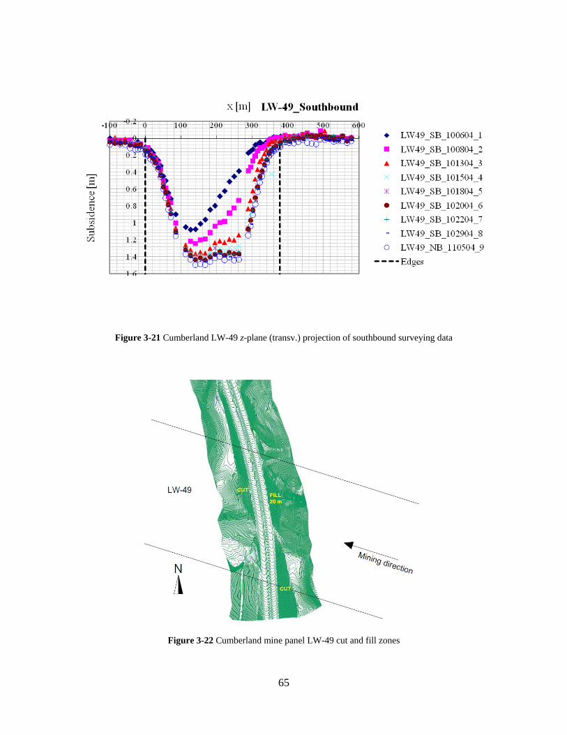
65
Figure 3-21 Cumberland LW-49 z-plane (transv.) projection of southbound surveying data
Figure 3-22 Cumberland mine panel LW-49 cut and fill zones

66
Figure 3-23 Cumberland LW-49 z-plane projection of northbound horizontal displacements
3.5.2 PANEL LW-51
Panel LW-51 is one of the best documented panels of this study. This fact is apparent from
Figure 3-26 and Figure 3-27, showing a total 9 different surveying dates, well spaced and
corresponding to mine face positions before the highway is reached, at locations underneath the
highway, and passed it, as illustrated in Figure 3-24. Figure 3-25 provides the highway elevation.
The southbound data corresponding to 05/04/2006 seems to differ from the general smooth
pattern. The data showed some abrupt change in the surface elevation as observed in Figure
3-27. This could very well be a result of deformation of highway fills. Figure 3-28 provides a
general topographic map with cut and fill zones. Figure 3-29 gives the final horizontal
displacements.

67
Figure 3-24 Overview of I-79 intersecting the projected Cumberland panel LW-51
Figure 3-25 Highway northbound elevation in the z-plane projection

68
Figure 3-26 Cumberland LW-51 z-plane (transv.) projection of northbound surveying data
Figure 3-27 Cumberland LW-51 z-plane (transv.) projection of southbound surveying data

69
Figure 3-28 Cumberland mine panel LW-51 cut and fill zones
Figure 3-29 Cumberland LW-51 z-plane projection of northbound horizontal displacements

70
3.5.3 PANEL LW-52
Panel LW-52 had a large data gap observed between the last two survey dates (Figure 3-30),
which will affect the transformed data as will be seen in section 3.7. Figure 3-31 provides the
highway elevation. Figure 3-32 and Figure 3-33 depict profiles from different dates on the
northbound and southbound of I-79. Substantial differences in maximum subsidence are apparent
in Figure 3-33 if the last profile is compared to that of the northbound. The shape of the final
transversal profile for the southbound does not resemble a typical supercritical profile, which
would be presumed to be more or less flat in the central region along the panel width. Instead, on
the right side of the panel a sharp rise in subsidence occurred giving an unusually high maximum
subsidence equal to 1.68 m. This behavior could very well be influenced by zones of highway
fills, similar to panel LW-51. Figure 3-34 gives a general topographic map with cut and fill
zones. Figure 3-35 depicts the final horizontal displacements.

71
Figure 3-30 Overview of Cumberland mine panel LW-52 intersecting I-79
Figure 3-31 Highway northbound elevation in the z-plane projection

72
Figure 3-32 Cumberland LW-52 z-plane (transv.) projection of northbound surveying data
Figure 3-33 Cumberland LW-52 z-plane (transv.) projection of southbound surveying data

73
Figure 3-34 Cumberland mine panel LW-52 cut and fill zones
Figure 3-35 Cumberland LW-52 z-plane projection of northbound horizontal displacements

74
3.5.4 PANEL LW-55
Panel LW-55 was added to the above mentioned PennDOT project as data became available
during and after mining, on the month of October 2008. This panel is unique in that it starts right
at the area of concern. Transformation of this data for supercritical-based prediction is not
relevant because a complete history until profiles became supercritical may not be obtained. One
reason is that the highway does not completely cross the panel and crosses close to a corner.
Another reason is the limitation of data, which were only measured until October 27 2008, as
shown in Figure 3-36. However, a small region of supercritical deformation may be observed in
Figure 3-37 and Figure 3-39, thus providing a valuable maximum subsidence magnitude. Figure
3-39 and Figure 3-40 show excessive heave taking place from 10/03/08 to 10/06/08 for the
southbound. A double-check of tiltmeter data seems to show no such drastic changes in
elevation, as depicted in Figure 3-42 and Figure 3-43.

75
Figure 3-36 Overview of Cumberland mine panel LW-55
Figure 3-37 Cumberland LW-55 x-plane (long.) projection of northbound surveying data

76
Figure 3-38 Cumberland LW-55 z-plane (transv.) projection of northbound surveying data
Figure 3-39 Cumberland LW-55 x-plane (long.) projection of southbound surveying data

77
Figure 3-40 Cumberland LW-55 z-plane (transv.) projection of southbound surveying data
Mining direction
N
LW-55
Figure 3-41 Overview of LW-55 tiltmeters

78
Figure 3-42 Cumberland mine panel LW-55 tiltmeter 3 elevation change readings
Figure 3-43 Cumberland mine panel LW-55 tiltmeter 5 elevation change readings
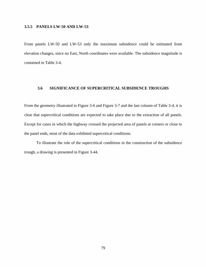
79
3.5.5 PANELS LW-50 AND LW-53
From panels LW-50 and LW-53 only the maximum subsidence could be estimated from
elevation changes, since no East, North coordinates were available. The subsidence magnitude is
contained in Table 3-4.
3.6 SIGNIFICANCE OF SUPERCRITICAL SUBSIDENCE TROUGHS
From the geometry illustrated in Figure 3-6 and Figure 3-7 and the last column of Table 3-4, it is
clear that supercritical conditions are expected to take place due to the extraction of all panels.
Except for cases in which the highway crossed the projected area of panels at corners or close to
the panel ends, most of the data exhibited supercritical conditions.
To illustrate the role of the supercritical conditions in the construction of the subsidence
trough, a drawing is presented in Figure 3-44.

80
Figure 3-44 Supercritical trough above a longwall panel
After the mining operation reaches the critical dimension Lc in the longitudinal direction,
subsidence experiences supercritical conditions. In all panels used here, this critical dimension is
also reached in the transversal (width) direction. Once this critical length is surpassed, and
provided that the rate of advance of the mine face is constant, the trough front that is formed
propagates like a wave in the direction of mining preserving its shape and advancing at roughly
the same rate at which the mine face progresses. This assumes that the overburden is
homogeneous and the mining operation remains steady. The reasonableness of the assumption is
illustrated in the data analysis.

81
Figure 3-45 shows two positions 1 and 2, representing two mine face positions with Position 2
farther advanced than Position 1. Both positions were reached after the critical dimension had
been surpassed. The assumption of the unchanged trough front advance is reflected in the shift of
the front.
Figure 3-45 The trough front in supercritical conditions

82
3.7 PROPOSED DATA TRANSFORMATION
After all subsidence values were obtained for each and every single station and coupled with the
position of the mine face for each surveying date, a transformation of the data was performed on
each panel that provided a sufficient amount of data. A step-by-step description of the process is
given here:
1. For every single station and every single date of surveying, subsidence, S, was
computed by subtracting the elevation from the baseline elevation.
2. For every single date, the position of the mine face was noted.
3. From the East, North, Elevation coordinate system, data was transformed into a
rotated coordinate system whose axes are parallel and perpendicular, respectively,
to the panel longitudinal direction (see Figure 3-24). The origin of this coordinate
system is the same as the East, North, Elevation, since the transformation involves
only rotation (clockwise at an angle of 17°32’53”). This coordinate system has
axes 1, 2, as shown in Figure 3-24.
4. In order to express point position locally for each panel in a convenient way, a
local coordinate system x, z, S, whose origin is located at the left end of the mine
face projected to the ground surface, was used for all stations available for each
surveying date (see Figure 3-46). The local x, z, S system moves as the mine face
advances. For the troughs that were within the supercritical region in the
longitudinal direction, with the adoption of homogeneous assumption, all these
data were combined in a 3D single x, z, S set.

83
Figure 3-46 Local coordinate system moving at the same rate as the mine face
Figure 3-47 through Figure 3-58 show transformed data for panel LW-51. Only a few positions
with respect to the mine face are shown, illustrating that a trough may be obtained. The farther
away from the mine face, the higher the magnitude of subsidence. It can be appreciated in Figure
3-58 that subsidence remains constant at the maximum potential magnitude after a certain
distance. This can also be seen in the longitudinal profiles obtained at the center of the panels,
shown in Figure 3-59 through Figure 3-62.

84
Figure 3-47 LW-51 transformed data between -610 m and -213 m from mine face
Figure 3-48 LW-51 transformed data between 0 m and 6.1 m from mine face

85
Figure 3-49 LW-51 transformed data between 30.5 m and 36.5 m from mine face
Figure 3-50 LW-51 transformed data between 61 m and 67 m from mine face

86
Figure 3-51 LW-51 transformed data between 91.4 m and 97.5 m from mine face
Figure 3-52 LW-51 transformed data between 121.9 m and 128 m from mine face

87
Figure 3-53 LW-51 transformed data between 152.4 m and 158.5 m from mine face
Figure 3-54 LW-51 transformed data between 170.7 m and 176.8 m from mine face
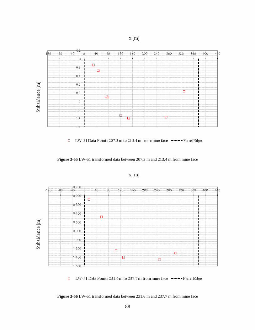
88
Figure 3-55 LW-51 transformed data between 207.3 m and 213.4 m from mine face
Figure 3-56 LW-51 transformed data between 231.6 m and 237.7 m from mine face

89
Figure 3-57 LW-51 transformed data between 268.2 m and 274.3 m from mine face
Figure 3-58 LW-51 transformed data between 213.4 m and 414.5 m from mine face

90
Figure 3-59 B-4 longitudinal subsidence profile in the central 210 m
Figure 3-60 Cumberland mine panel LW-49 longitudinal profile for the central 120 m

91
Figure 3-61 Cumberland mine panel LW-51 longitudinal profile for the central 120 m
Figure 3-62 Cumberland mine panel LW-52 longitudinal profile for the central 120 m

92
4.0 DEVELOPING AN EMPIRICAL SUBSIDENCE PREDICTION MODEL
The previous chapter provided a general description of surveying data and a description of a
transformation process that allows expressing the subsidence trough as a spatial function in
supercritical subsidence deformation regions along the longwall panel.
The representation of the subsidence trough of a given longwall panel in terms of point
coordinates and subsidence magnitude is a very useful result. Its deformation magnitudes are
geology dependent and tied to the geometric characteristics of the given panel, such as width of
the panel, extraction thickness, and overburden thickness.
The present chapter introduces the proposed methodology to empirically obtain any
supercritical subsidence trough by taking the overburden thickness, extraction thickness, and
panel width into consideration. It is important to emphasize at this point that any empirical model
based upon data of a given geology shall serve as a prediction tool for the same geology from
which the data were obtained.
The proposed methodology considers two main stages as described in section 3.3. The
first stage consists of a maximum subsidence model. The second stage consists of a normalized
subsidence distribution model.

93
4.1 MAXIMUM SUBSIDENCE PREDICTION
In this dissertation, all panels reached supercritical subsidence conditions, which implies that
maximum potential subsidence fully develops. Researchers report that the subsidence factor, a,
as defined in chapter 2.0 , reaches a constant value for the case of supercritical conditions, given
the geology doesn't change (NCB 1975; Whittaker and Reddish 1989; Agioutantis and Karmis
2009). Peng, however, provides an inverse relationship between maximum potential subsidence
factor and overburden depth based upon several Appalachian sites (Peng 1992), suggesting that
the depth of the mine has a direct influence on the magnitude of subsidence. An accompanying
explanation by Peng on this relationship claims that as depth increases, the area of influence of
the extraction increases, producing milder subsidence and also decreased deformation indices
that result along with subsidence. The relationship found in this study supports the findings by
Peng.
Figure 4-1 gives the relationship between subsidence factor and overburden thickness,
based on the data from Table 3-1.
The model illustrates that the ultimate absolute magnitude of maximum potential
subsidence is a function of overburden thickness and extraction thickness. This relationship
alone is a very useful predictive tool as far as the maximum subsidence magnitude is concerned.
The two parameters it is based on are generally available.

94
Figure 4-1 Highway maximum subsidence model in Greene County
4.2 NORMALIZED SUBSIDENCE DISTRIBUTION MODEL
The previous section described a model to obtain maximum potential subsidence. Even though it
is a very simple and useful model for practical applications, it is not capable of providing
information such as the distribution of subsidence near the edges, and the consequent
deformation indices that are required to be quantified for proper prediction and control.
In order to achieve the final stage of subsidence trough prediction, surface distribution of
normalized subsidence is required. In order to obtain a generic distribution, both the magnitude
of subsidence at a point and its surface location need to be normalized.

95
4.2.1 Subsidence normalization
Given a distribution of absolute subsidence readings like that obtained after data transformation
and illustrated in Figure 3-47 through Figure 3-58, all readings may be normalized with respect
to the maximum subsidence, S*, obtained from the maximum subsidence model described in
section 4.1.
4.2.2 Lateral position normalization or edge effect
The lateral normalization or edge effect normalization is obtained by normalizing the lateral
distance of every point measured from the panel edges. The parameter by which this lateral
normalization is carried out is the overburden depth, H. Performing the normalization of lateral
location x, z, with respect to H, is equivalent to considering the edge effect of subsidence
deformation. This can be seen for example in the prediction of the location of the inflection point
as a function of the ratio W/H in SDPS (Agioutantis and Karmis 2009). Beyond W/H = 1.2, d/H
becomes constant. This suggests that normalizing the abscissas of our data with respect to the
overburden depth, H, would bring all supercritical profiles together in the inflexion point. Figure
4-2 and Figure 4-3 depict the transversal and longitudinal normalized subsidence profiles,
respectively.

96
Figure 4-2 Normalized subsidence and normalized location in the transverse direction
Figure 4-3 Normalized subsidence and normalized location in the longitudinal direction

97
4.3 FITTING A 3D MODEL
The previous section described how data can be normalized both vertically and horizontally and
showed that the data available follow convenient trends when normalized. That is, narrow
bounds are formed in normalized data. This leads to the next step, which is fitting a three-
dimensional normalized subsidence model to the data.
In order to obtain a 3D model, a transverse 2D model and a longitudinal 2D model will
be multiplied. Two-dimensional models are common in the literature. One of them has been
described in chapter 2.0 (Agioutantis and Karmis 2009).
A transversal view of 3D data for all panels is shown in Figure 4-4. The view presented is
from the mined area toward the mine face. Each point is at a unique distance away from the mine
face, and some trends can be observed that stand for data taken on a given date along I-79. The
procedure to obtain data in x, z, S (transversal, longitudinal, subsidence) has been explained in
section 3.7. In summary, what can be visualized in this figure is the 2D-projected subsidence
trough to which a 3D function can be fitted. The function, or model, will have to address the
following factors:
• Panels do not have the same width.
• Some panels are symmetric in the case that no adjacent panel has been previously mined
out in the immediate neighborhood (e.g. LW-49).
• Some panels exhibit asymmetry, that is, the side adjacent to a mined-out panel is more
subsided than the opposite side, etc.
These features, however, are easy to deal with, as long as a good model can be found to
describe the complex shape of the typical edge deformations, whether these are adjacent to
mined-out or not mined-out panels. The symmetric and asymmetric trends that appear in Figure

98
4-4 are depicted separately for a symmetric case (LW-49 in Figure 4-5) and an asymmetric case
(LW-52 in Figure 4-6). The model proposed here will be capable of predicting either case, unlike
any other subsidence prediction tool developed in the past. Figure 4-7 through Figure 4-10 show
data according to its use as symmetric side (without mined-out adjacent panel) or asymmetric
side (with mined-out panel adjacent).
-0.2
0
0.2
0.4
0.6
0.8
1
1.2
-0.6 -0.4 -0.2 0 0.2 0.4 0.6 0.8 1 1.2 1.4 1.6 1.8 2
x/H
S/S*
Figure 4-4 Transversal view of data from all panels

99
Figure 4-5 Final subsidence for symmetric case LW-49
Figure 4-6 Final subsidence for asymmetric case LW-52

100
-0.2
0
0.2
0.4
0.6
0.8
1
1.2
-0.6 -0.4 -0.2 0 0.2 0.4 0.6 0.8 1
x/H
S/S*
Figure 4-7 Transversal view of panels LW-49, 51, 52 data adjacent to non-mined-out panel
-0.2
0
0.2
0.4
0.6
0.8
1
1.2
-0.6 -0.4 -0.2 0 0.2 0.4 0.6 0.8 1 1.2
x/H
S/S*
Figure 4-8 LW-49, 51, 52 transversal final deformation adjacent to non-mined-out panel

101
-0.2
0
0.2
0.4
0.6
0.8
1
1.2
0 0.2 0.4 0.6 0.8 1 1.2 1.4 1.6 1.8
x/H
S/S*
Raw data adjacent to mined-out panel
Rotated data with respect to panel center
Figure 4-9 LW-51, 52 transversal raw and rotated data adjacent to mined-out panel
0
0.2
0.4
0.6
0.8
1
1.2
0 0.2 0.4 0.6 0.8 1 1.2 1.4 1.6 1.8
x/H
S/S*
Raw data adjacent to mined-out panel
Rotated data with respect to panel center
Figure 4-10 LW-51, 52 transversal final deformation data adjacent to mined-out panel

102
The problem of fitting data with a 3D profile function requires a non-linear regression technique.
Since the data trends are clear, the search for functions to fit the data is relatively
straightforward. For the non-linear regression, a Genetic Algorithm (GA), which is a robust
search technique in determining the parameters of the proposed model, will be used. After
specifying a profile function, an objective function, and giving a range of possible parameter
values, the GA finds parameter values that provide a global minimum fit according to the
objective functions.
For this dissertation, the objective is to find the parameters of the model such that the
sum of squared errors between the model and data is minimum. Thus, the objective function is
simply a function that defines the sum of squared errors.
Investigations have been made on four different 3-D profile models in this work. The first
model has the following form:
a6a3
Hza5a4
Hxa2a1
ee*S
S −−= 4-1
The model in 4-1 is similar to the model proposed by Chen and Peng of West Virginia
University (OSMRE 1986).
+−
+−
−−=Hza4a3
Hxa2a1
ee ee*S
S 4-2
The second model (4-2) is called the Gompertz model in its 2D version (Graybill and Iyer 1994)
and has not been employed in subsidence prediction before.
+−
+−=
Hza4a3tanh1
Hxa2a1tanh10.25
*SS
4-3

103
The third model (4-3) would be the 3D version of the subsidence profile function used by SDPS
(Agioutantis and Karmis 2009).
a6
Hza5a4
a3
Hxa2a1
e1e1
1*S
S
+
+
=
+−
+−
4-4
The fourth model (4-4) is known as Richard’s model (Graybill and Iyer 1994) in its 2D
version, and as model 4-2, it has not been used in the past for subsidence prediction either. All
these models in their 2D version are capable of dealing with profile fitting in the problem of
subsidence. Usually the 2D problem involves estimation of maximum or final subsidence, for
which a supercritical final deformed profile is fit usually by taking the transversal coordinate as
the horizontal distance. However, the 3D problem that arises from the data depicted in Figure 4-4
through Figure 4-10 imposes the challenge of dealing with both final deformations (large and far
from mine face) and dynamic deformations (small and close to mine face) through a single 3D
regression model. Runs of the GA algorithm for everyone and each of the above four models
show that two of the models, i.e. models 1 and 4, each having 6 model parameters (namely
models equation 4-1 and equation 4-4) best fit the data. This is not surprising since dealing with
the 3D nature of the data requires a level of detail that the 6 parameter models are much more
capable of accounting for than the 4-parameter models. Table 4-1 and Table 4-2 contain the
output of parameters for the various regression models, together with the objective function
value and standard deviation. Trial function number 4 (4-4) proved to best fit the data.

104
Table 4-1. Genetic algorithm output for side without adjacent panel
Trial function a1 a2 a3 a4 a5 a6
Sum of squared
error n p Standard
Deviation
1 0.00 1.93 16.04 0.00 2.42 9.67 10.2 1264 6 0.090 2 -2.72 2.57 -0.35 -0.19 87.2 1264 4 0.263 3 1.32 -5.58 1.94 -2.81 111.3 1264 4 0.297 4 -2.79 11.60 1.24 -1.94 5.99 1.23 8.5 1264 6 0.082
Table 4-2. Genetic algorithm output for side with adjacent panel
Trial function a1 a2 a3 a4 a5 a6
Sum of squared
error n p Standard
Deviation
1 0.00 2.06 13.23 0.00 2.14 10.87 0.89 628 6 0.038 4 -1.83 10.34 1.11 -1.45 6.73 2.23 0.73 628 6 0.034
When the asymmetrical model is used, however, it is still desired that the two model halves
match along a central line smoothly. Therefore, the parameters a4, a5, a6 may be set equal to
those of the symmetric model (longitudinal, z, parameters), leaving only the transversal
parameters a1, a2, a3 as variables. Setting the former constant and equal to -1.94, 5.99, and 1.23,
and re-running the genetic algorithm, the results in Table 4-3 are obtained, which are still very
good results.
Table 4-3. Genetic algorithm output for side with adjacent panel Trial function 4
Trial function a1 a2 a3 a4 a5 a6
Sum of squared
error n p Std.
Dev.
4 -2.77 12 0.73 -1.94 5.99 1.23 0.92 628 6 0.038

105
4.4 SPATIAL DISTRIBUTION OF SUBSIDENCE
The previous sections of this chapter described the way empirical relationships can serve the
purpose of three-dimensional subsidence prediction by using the maximum subsidence model
and the non-linear regression proposed for normalized data.
The first stage, which is concerned with the estimation of maximum potential subsidence,
is achieved using the maximum subsidence model and obtaining maximum subsidence, S*, as a
function of extraction thickness, M, and overburden thickness, H.
The second stage is to use the non-linear model, by plugging in the overburden thickness,
H, and the maximum subsidence, S*, to obtain the subsidence trough. In step-wise form, spatial
distribution of subsidence is obtained following the two steps:
1. S*/M is read as a function of H. S* is thus obtained by multiplying S*/M by M.
2. The non-linear model (e.g. without mined adjacent panel) is evaluated by
plugging in H and S*:
1.23
Hz..
1.24
Hx..
e1e1
1*S
S
+
+
=
+−−
+−− 9959416011792
4-5
An example of the use of this model is illustrated by its application on panel LW-51 and depicted
in Figure 4-11 through Figure 4-22.

106
Figure 4-11 LW-51 subsidence prediction between -610 m and -213 m from mine face

107
Figure 4-12 LW-51 subsidence prediction between 0 m and 6.1 m from mine face
Figure 4-13 LW-51 subsidence prediction between 30.5 m and 36.5 m from mine face

108
Figure 4-14 LW-51 subsidence prediction between 61 m and 67 m from mine face
Figure 4-15 LW-51 subsidence prediction between 91.4 m and 97.5 m from mine face

109
Figure 4-16 LW-51 subsidence prediction between 121.9 m and 128 m from mine face
Figure 4-17 LW-51 subsidence prediction between 152.4 m and 158.5 m from mine face

110
Figure 4-18 LW-51 subsidence prediction between 170.7 m and 176.8 m from mine face
Figure 4-19 LW-51 subsidence prediction between 207.3 m and 213.4 m from mine face

111
Figure 4-20 LW-51 subsidence prediction between 231.6 m and 237.7 m from mine face
Figure 4-21 LW-51 subsidence prediction between 268.2 m and 274.3 m from mine face

112
Figure 4-22 LW-51 subsidence prediction between 213.4 m and 414.5 m from mine face
4.5 TEMPORAL DISTRIBUTION OF SUBSIDENCE
One apparent feature of the way the trough is obtained is that the trough front, as it is described,
experiences the dynamic effect of subsidence. In other words, if the non-linear regression that
describes the trough is evaluated at the panel center and a central longitudinal profile is obtained,
that longitudinal profile is nothing but the dynamic subsidence profile. Provided the geology is
the same, the shape of the dynamic subsidence profile is influenced by the rate of advance of the
mine face and it can be gentle for high rates of advance or sharp for slow rates (Kratzsch 1983;
Jarosz, Karmis et al. 1990; Kratzsch 2008; Agioutantis and Karmis 2009).

113
The data upon which the 3D model is based comes from three panels, LW-49, LW-51, and LW-
52, which experienced an average constant rate of advance of roughly 17 m/day. As a result, the
non-linear regression here obtained represents the magnitude of or close magnitudes to that rate
of advance. The difference between the dynamic profile shape and the permanent deformation
shapes on the sides of the panel, or static profiles as they are often called, is clear if Figure 4-2
and Figure 4-3 are compared. One way to deal with intermediate values of rate of advance
between 0 and 17 m/day would be to consider profiles interpolated within these two limits. For
rates of advance higher than 17 m/day, the prediction could be less reliable, although conclusions
on this may not be drawn due to a lack of data.
In temporal subsidence prediction, a useful task is to predict deformation for a given
point in terms of a time scale that can be set to zero for the position of the mine face. The basic
assumption for both spatial and temporal subsidence prediction is that the rate of mine face
advance is constant, and in this case equal to 17 m/day. Therefore, the longitudinal coordinate, z,
can be expressed as a function of the rate of advance, v, as vtz = .
1.23
Ht..
1.24
Hx..
e1e1
1*S
S
+
+
=
+−−
+−− 831019416011792
4-6
Since v = 17 m/day, the spatial coordinate z is replaced by 17t, and the model in 4-6 is obtained.
Since t = 0 corresponds to the mine face position, t < 0 corresponds to points ahead of the mine
face, whereas t > 0 corresponds to points behind the mine face. For example, if there are
concerns about a point P that is estimated to be reached by the mine face in 4 days, its
deformation can be predicted for the days before and after the mine face passes by plugging in t
= -3, -2, -1, 0, 1, 2, 3. It is important to note that the model 4-6 has the spatial coordinate x as one
of its independent variables. This is useful since the point P of concern could be located

114
anywhere within the width of the panel, even outside the edges. Also, complete transverse
profiles could be predicted for different times.
Another way the temporal subsidence may be looked at is in the prediction of long-term
subsidence, for which researchers have proposed decay functions (Whittaker and Reddish 1989).
This work is not concerned with this type of prediction since the available data was obtained
soon after the mine face passed the surveyed stations.
4.6 SUBSIDENCE DEFORMATION INDICES
Definitions of subsidence deformation indices were introduced in section 1.3 and illustrated in
Figure 1-3. Information indices are important for damage prediction. If the subsidence profile or
trough is known, these can be easily obtained.
From the general model, left half:
654
321
a
Hzaa
a
Hxaa
e1e1
*SS
+
+
=
+−
+−
4-7
the following parts may be defined:
321
a
Hxaa
X
e1
*SC
+
=
+−
4-8
654
a
Hzaa
Z
e1
*SC
+
=
+−
4-9

115
321
a
Hxaa
X
e1
1S
+
=
+−
4-10
654
a
Hzaa
Z
e1
1S
+
=
+−
4-11
The first and second derivatives of 4-10 and 4-11 are required for the deformation indices. The
expressions for the case of the transversal direction, x, left half, are:
1a
Hxaa
Hxaa
32X 3
21
21
e1
eHaaS' +
+−
+−
+
= 4-12
+
+−=
−−
+−
+−
1a
Hxaa
Hxaa
23
22
X
32121
e1eH
aa'S'
( )2a
Hxaa
Hxaa2
23
223
32121
e1eH
aa1a−−
+−
+−
+
+ 4-13
For the right half:
( )
( ) 1a
Hx-Waa
Hx-Waa-
32X 3
21
21
e1
eHaaS' +
+−
+
+
−=
4-14
( ) ( )
+
+−=
−−
+
+
1a
Hx-Waa-
Hx-Waa-
23
22
X
32121
e1eH
aa'S'
( ) ( ) ( ) 2a
Hx-Waa
Hx-Waa2
23
223
32121
e1eH
aa1a−−
+−
+−
+
+
4-15

116
The same expressions may be obtained for the longitudinal direction, z. Based on these, the
deformation indices are defined as follows:
XZX S'CxSSlope =∂∂
=
4-16
XZ2X 'S'CxSCurvature −=
∂∂
−=2
4-17
As discussed in subsection 1.3.3, horizontal displacements are correlated to slope through a
constant. The SDPS developers (Agioutantis and Karmis 2009) use a factor Bf defined as
tanβHBBf = , where B is a fitting constant and
tanβH is the radius of influence, where H is the
overburden thickness and β is the angle of influence. The SDPS uses B = 0.35 for Northern
Appalachia. From horizontal displacement figures, given by Figure 3-16, Figure 3-23, Figure
3-29, and Figure 3-35, however, and taking the resulting subsidence trough into account, a value
for this constant B is set here equal to 0.15. Figure 4-23 through Figure 4-31 give a graphical
example of the application of the new model in the symmetric case of LW-49.

117
Figure 4-23 Subsidence trough of symmetric case LW-49 obtained with new model
Figure 4-24 Distribution of transversal (x) slope for symmetric case LW-49
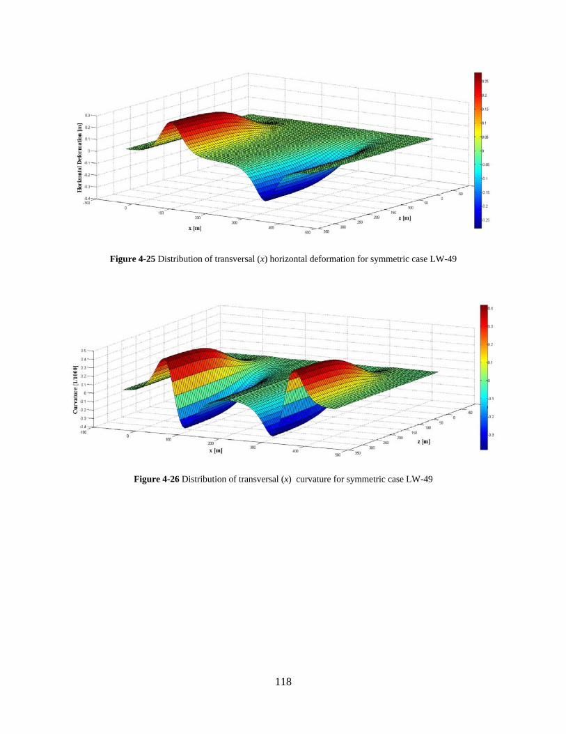
118
Figure 4-25 Distribution of transversal (x) horizontal deformation for symmetric case LW-49
Figure 4-26 Distribution of transversal (x) curvature for symmetric case LW-49

119
Figure 4-27 Distribution of transversal (x) horizontal strain for symmetric case LW-49
Figure 4-28 Distribution of longitudinal (z) slope for symmetric case LW-49

120
Figure 4-29 Distribution of longitudinal (z) hor. deformation for symmetric case LW-49
Figure 4-30 Distribution of longitudinal (z) curvature for symmetric case LW-49
Figure 4-31 Distribution of longitudinal (z) horizontal strain for symmetric case LW-49

121
4.7 COMMENTS ON HORIZONTAL DISPLACEMENTS
A three-dimensional trough subsidence may be predicted as described in previous sections of this
chapter. Section 4.6 introduced the traditional way horizontal displacements are dealt with. A
linear correlation to slope yields horizontal displacement, an assumption so generalized that
seems to have worked well for relatively flat terrain. Some researchers, however, have brought
up the fact that this assumption is less reliable when hilly terrain is dealt with (Luo and Peng
1999), and have proposed methodologies to account for the inclination of terrain and its impact
both on subsidence and horizontal displacements. Luo and Peng, for example, consider the
proportionality factor G, which is the reciprocal of the safety factor against sliding of an infinite
slope (Luo and Peng 1999). Their paper shows an example where this assumption seems to
work. Basically, a relatively shallow topsoil above the bedrock is considered, and its tendency to
slide as a function of the terrain slope, represented by the G factor, is considered in adjusting the
subsidence movements caused by a flat terrain.
The behavior provided by the data of the present work, however, seems to be quite
different, as suggested by Figure 3-16, Figure 3-23, Figure 3-29, and Figure 3-35. In general, it
may be observed that horizontal displacements experienced by the highway foundation are
sensitive to very gentle highway gradients of the order of 1 to 3 degrees. In cases where the
direction of highway gradient is constant, that is, the whole highway segment above the panel
width going uphill or downhill, it is possible that almost all surveyed points move in a single
direction, namely the downhill direction. This behavior cannot be captured by the assumption
that horizontal displacements may be correlated to the trough slope. Also, considering infinite
slope stability does not seem to be the best approach since the behavior is dominated by complex

122
irregular three-dimensional geometry. The complex behavior of horizontal displacements on top
of highway foundations will be addressed in the numerical modeling part of this work.

123
5.0 HIGHWAY SUBSIDENCE FINITE ELEMENT MODEL
A Finite Element Model (FEM) for the problem of highway subsidence is proposed here. Table
5-1 gives a list of the actual rock layers encountered in the field, according to a 1955 boring log
by Mott Core Drilling Company in Perry Township, Greene County, and their thicknesses, as
well as a set of layers used in the finite element model.
Table 5-1 Boring log and FEM model layer thicknesses
Sub-layer No.
(bottom-up)
Approx. thickness of individual layers [ft]
Approx. thickness of individual
layers [m] Depth [m] Rock type FEM Layer
(bottom-up)
Total layer thickness
[m]
55 5.0 1.5 1.5 Surface 29 4.0 54 6.0 1.8 3.4 Brown clay
53 12.0 3.7 7.0 Gray shale 28 4.0
52 40.5 12.3 19.4 Gray sandy shale 27 12.0
51 17.5 5.3 24.7 Dark shale 26 5.0
50 3.4 1.0 25.7 Sandy shale 25 3.0 49 6.5 2.0 27.7 Gray shale
48 1.4 0.4 28.1 Coal
47 20.0 6.1 34.2 Dark shale 24 8.0
46 1.0 0.3 34.5 Coal 23 5.0 45 12.6 3.8 38.4 Sandy shale
44 3.5 1.1 39.4 Dark shale 43 52.5 16.0 55.4 Sandy lime
22 18.0 42 7.2 2.2 57.6 Sandstone 41 10.3 3.1 60.8 Gray lime
21 7.0 40 2.5 0.8 61.5 Sandy lime 39 7.0 2.1 63.7 Gray lime 38 3.7 1.1 64.8 Coal

124
Table 5-1 (Continued)
Sub-layer No. (bottom-
up)
Aprox. thickness of individual layers [ft]
Aprox. thickness of individual
layers [m] Depth [m] Rock type FEM Layer
(bottom-up)
FEM Total layer
thickness [m]
37 4.6 1.4 66.2 Green lime 20 4.0 36 10.0 3.0 69.3 Green soft lime
35 35.7 10.9 80.1 Sandstone 19 11.0
34 20.0 6.1 86.2 Dark shale 18 8.0 33 7.2 2.2 88.4 Coal
32 10.0 3.0 91.5 Sandy shale 17 6.0 31 3.2 1.0 92.4 Sandstone
30 5.0 1.5 94.0 Dark shale
29 15.5 4.7 98.7 Gray lime 16 5.0
28 10.3 3.1 101.8 Green lime 15 5.0 27 5.5 1.7 103.5 White lime
26 15.4 4.7 108.2 Green lime 14 5.0
25 10.3 3.1 111.3 White lime 13 7.0 24 14.2 4.3 115.7 Gray lime
23 36.0 11.0 126.6 White lime 12 11.0
22 25.5 7.8 134.4 Sandy lime 11 8.0
21 7.3 2.2 136.6 White lime 10 12.0 20 32.7 10.0 146.6 Lime shale streaks
19 12.0 3.7 150.3 White lime 9 4.0
18 4.4 1.3 151.6 Dark shale 8 9.0 17 10.4 3.2 154.8 Gray lime
16 3.2 1.0 155.8 Green lime 15 12.0 3.7 159.4 Gray lime
14 13.0 4.0 163.4 Sandy shale 7 6.0 13 4.4 1.3 164.7 Dark shale
12 3.8 1.2 165.9 Coal
11 17.0 5.2 171.1 Dark shale 6 5.0
10 24.5 7.5 178.5 Sandy shale 5 7.0
9 3.0 0.9 179.4 Dark shale 4 5.3 8 2.0 0.6 180.0 Soft clay
7 1.1 0.3 180.4 Coal 6 2.0 0.6 181.0 Dark shale
5 6.6 2.0 183.0 Gray lime 3 5.3 4 14.2 4.3 187.3 Dark shale
3 7.6 2.3 189.6 Bone coal streaks
2 7.4 2.3 191.9 Coal 2 2.4
1 131.2 40.0 231.9 Floor 1 40.0
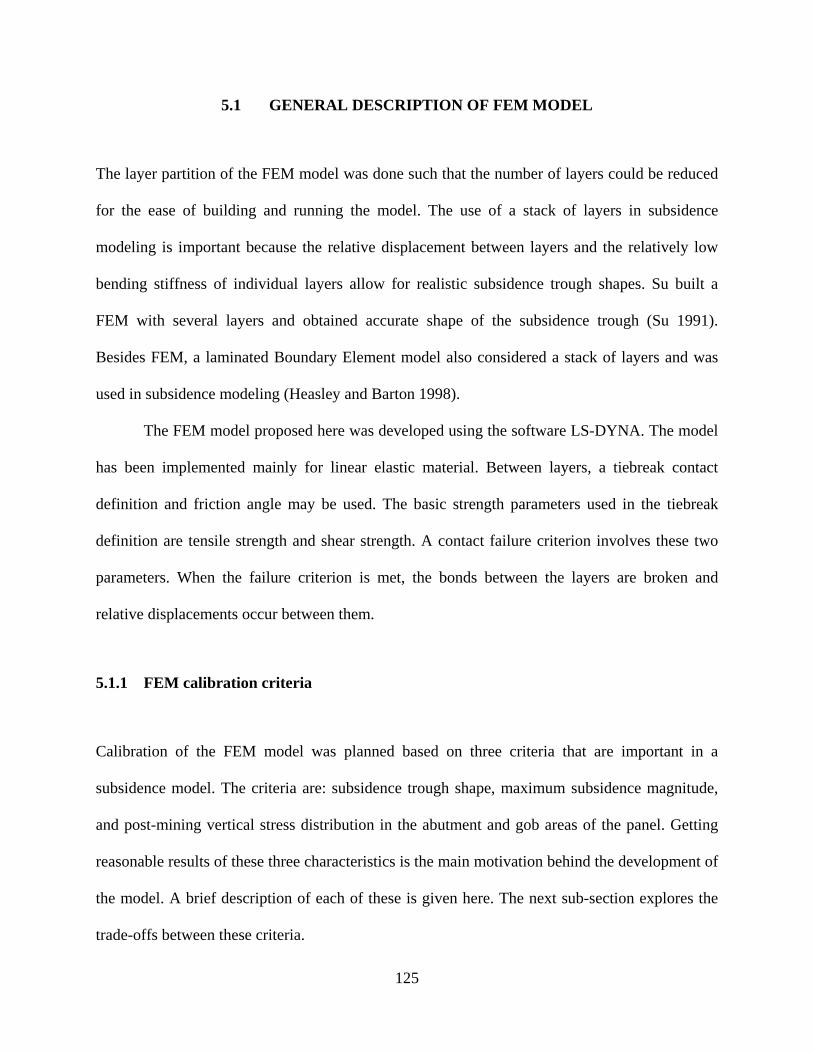
125
5.1 GENERAL DESCRIPTION OF FEM MODEL
The layer partition of the FEM model was done such that the number of layers could be reduced
for the ease of building and running the model. The use of a stack of layers in subsidence
modeling is important because the relative displacement between layers and the relatively low
bending stiffness of individual layers allow for realistic subsidence trough shapes. Su built a
FEM with several layers and obtained accurate shape of the subsidence trough (Su 1991).
Besides FEM, a laminated Boundary Element model also considered a stack of layers and was
used in subsidence modeling (Heasley and Barton 1998).
The FEM model proposed here was developed using the software LS-DYNA. The model
has been implemented mainly for linear elastic material. Between layers, a tiebreak contact
definition and friction angle may be used. The basic strength parameters used in the tiebreak
definition are tensile strength and shear strength. A contact failure criterion involves these two
parameters. When the failure criterion is met, the bonds between the layers are broken and
relative displacements occur between them.
5.1.1 FEM calibration criteria
Calibration of the FEM model was planned based on three criteria that are important in a
subsidence model. The criteria are: subsidence trough shape, maximum subsidence magnitude,
and post-mining vertical stress distribution in the abutment and gob areas of the panel. Getting
reasonable results of these three characteristics is the main motivation behind the development of
the model. A brief description of each of these is given here. The next sub-section explores the
trade-offs between these criteria.

126
5.1.1.1 Subsidence trough shape
The shape of the subsidence trough is a very important feature in a prediction model.
Underground extractions in materials that behave somewhat elastically will produce S-shapes in
the surface when the extractions reach certain dimensions. However, the S-shaped subsidence
curve needs to be accurate if the model is intended to serve prediction of surface deformations,
as the location of critical deformations needs to be known. The key to the correct shape of
subsidence troughs is the stacking of several thin layers that represent the geologic strata in the
overburden rock. The correct shape of a subsidence trough can be calibrated trough appropriate
number of layers, relative thickness of the layers with respect to overburden depth, mechanical
properties of the layer material, and strength of the bonding between layers.
5.1.1.2 Maximum subsidence
The problem of predicting maximum subsidence has been discussed and a maximum subsidence
model for the region has been proposed (see Figure 4-1). For this purpose, the ratio of maximum
subsidence to extraction thickness, S*/M, was used, which is always less than 1.0 and in the
vicinity of 0.67. An important factor that contributes to this ratio being always less than 1.0 is the
bulking factor. Peng defines the bulking factor as "the ratio of the volume of the broken rock
strata to the original volume of the same strata before they are broken and cave." It continues:
"Since the volume of the broken strata is always larger than that of the original intact strata,
bulking factor is usually larger than one" (Peng 2008).
The average value of bulking factor measured by Peng was 1.28. The bulking behavior of
broken rock is a feature not considered in the present FEM model. Even though LS-DYNA has
the capabilities necessary to model damage in rock materials, its implementation in the problem
of three-dimensional subsidence would be computationally extremely expensive and impractical.

127
Obtaining magnitudes of subsidence in supercritical troughs that are less than the extracted
thickness is a very difficult task without considering the bulking factor. Even though it is still
possible to get the correct value of the S*/M ratio if the roof of the extracted cavity is not allowed
to touch the floor, the resulting distribution of vertical stress in the abutment and gob areas and
the trough shape so obtained are not satisfactory.
5.1.1.3 Post-mining vertical stress distribution in abutment and gob areas
The model would be expected to give not only correct subsidence magnitude and shape, but also
a reasonably correct redistribution of post-mining vertical stresses in the abutment and gob areas.
This would consistently connect what is happening in the mine with what is happening in the
surface. Otherwise, many different combinations of parameters could be used to produce correct
subsidence magnitudes and shapes without truly representing the mechanics of the problem.
Typical abutment and gob stress distributions are given in Figure 5-1 and Figure 5-2 (Morsy and
Peng 2002).
Figure 5-1 Qualitative abutment stress distribution

128
Figure 5-2 Probable distribution of strata pressure in the vicinity of the longwall face
(Morsy and Peng 2002)
5.1.2 Trade-off between subsidence shape, subsidence magnitude, and post-mining
vertical stress redistribution
The model investigation begins with a stack of relatively thin layers whose thicknesses are given
in Table 5-1. Several cases will be explored in which the role of each of the three calibration
criteria is analyzed.
5.1.2.1 Case 1
The modulus of elasticity for all layers is equal to 1.48x10¹⁰ Pa and the Poisson's ratio is equal to
0.22. The tensile and shear interface bond strengths were varied linearly from the top to the
bottom in the range 2.35x10⁶ Pa to 5.35x10⁶ Pa, for an average of 3.95x10⁶ Pa for the first case,

129
roughly 10% of the compressive strength of a typical rock encountered in this region. This first
model is given in Figure 5-3. S*/M turned out to be equal to 1.09 because the layers fall into the
created extraction, thus fully closing the vertical gap. The readings of subsidence were corrected
by subtracting the initial settlement due to the application of gravity to the whole model.
Figure 5-3 Subsidence for case 1
The shape of the trough obtained with this first model is given in Figure 5-4. In terms of shape, it
can appreciated that the stacking of thin layers is very effective and a very accurate shape may be
obtained.

130
Figure 5-4 Shape of subsidence trough for case 1
The post-mining redistribution of stresses is given in Figure 5-5. Since the central portion of the
stack of layers is allowed to fall downward with all of its weight applied on the floor of the
cavity, the magnitude of the stresses is essentially the same in the gob as in the abutments.
Figure 5-5 Post-mining vertical stress redistribution for case 1

131
5.1.2.2 Case 2
In case 2, the modulus of elasticity for all layers is also equal to 1.48x10¹⁰ Pa and the Poisson's
ratio is equal to 0.22. The tensile and shear interface bond strengths were varied linearly from the
top to the bottom in the range 2.40x10⁶ Pa to 5.60x10⁶ Pa, for an average of 4.00x10⁶ Pa for the
first case, just a slight increase with respect to case 1. This second model is given in Figure 5-6.
S*/M turned out to be equal to 1.07 because the layers fall into the created extraction, thus fully
closing the vertical gap. The readings of subsidence were corrected by subtracting the initial
settlement due to the application of gravity to the whole model.
Figure 5-6 Subsidence for case 2
The shape of the trough obtained with the second model is given in Figure 5-7. In terms of shape,
it can appreciated that the stacking of thin layers is very effective and a very accurate shape may
be obtained.

132
Figure 5-7 Shape of subsidence trough for case 2
The post-mining redistribution of stresses is given in Figure 5-8. Since the central portion of the
stack of layers is allowed to fall downward with all of its weight applied on the floor of the
cavity, the magnitude of the stresses is essentially the same in the gob as in the abutments.

133
Figure 5-8 Post-mining vertical stress redistribution for case 2
5.1.2.3 Case 3
In case 3, the modulus of elasticity for all layers is also equal to 1.48x10¹⁰ Pa and the Poisson's
ratio is equal to 0.22. The tensile and shear interface bond strengths were varied linearly from the
top to the bottom in the range 2.45x10⁶ Pa to 5.65x10⁶ Pa, for an average of 4.05x10⁶ Pa for the
first case, again a very slight increase with respect to case 2. This second model is given in
Figure 5-6. S*/M in this model goes abruptly down to 0.24 as the whole stack of layers remains
hanging in the central portion and supported only in the abutments. The readings of subsidence
were corrected by subtracting the initial settlement due to the application of gravity to the whole
model.

134
Figure 5-9 Subsidence for case 3
The shape of the trough obtained with the third model is very flat, as given in Figure 5-10.

135
Figure 5-10 Shape of subsidence trough for case 3
The post-mining redistribution of stresses is given in Figure 5-11. Since the central portion of the
stack of layers is not touching the floor of the cavity, the magnitude of the stresses in the
abutments is high whereas the central part of the overburden is in tension.
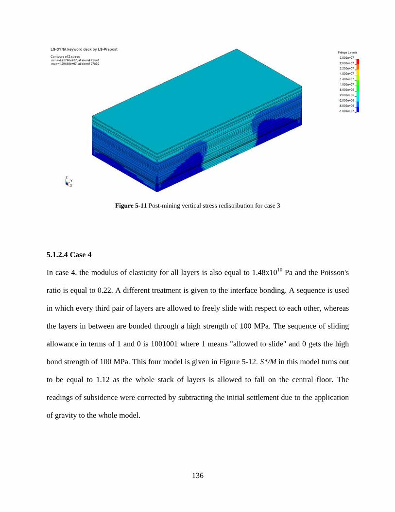
136
Figure 5-11 Post-mining vertical stress redistribution for case 3
5.1.2.4 Case 4
In case 4, the modulus of elasticity for all layers is also equal to 1.48x10¹⁰ Pa and the Poisson's
ratio is equal to 0.22. A different treatment is given to the interface bonding. A sequence is used
in which every third pair of layers are allowed to freely slide with respect to each other, whereas
the layers in between are bonded through a high strength of 100 MPa. The sequence of sliding
allowance in terms of 1 and 0 is 1001001 where 1 means "allowed to slide" and 0 gets the high
bond strength of 100 MPa. This four model is given in Figure 5-12. S*/M in this model turns out
to be equal to 1.12 as the whole stack of layers is allowed to fall on the central floor. The
readings of subsidence were corrected by subtracting the initial settlement due to the application
of gravity to the whole model.

137
Figure 5-12 Subsidence for case 4
The shape of the trough obtained with the fourth model is given in Figure 5-13. The shape again
looks correct as sliding is allowed in some interfaces and the central portion of the rock falls into
the ground.

138
Figure 5-13 Shape of subsidence trough for case 4
The post-mining redistribution of stresses is given in Figure 5-14. Since the central portion of the
stack of layers is allowed to fall downward with all of its weight applied on the floor of the
cavity, the magnitude of the stresses is essentially the same in the gob as in the abutments.

139
Figure 5-14 Post-mining vertical stress redistribution for case 4
5.1.2.5 Case 5
Case 5 is like case 4, except for the sequence of sliding allowance. In this case, this sequence is
100010001. This fifth model is given in Figure 5-15. S*/M in this model turns out to be equal to
1.06 as the whole stack of layers is still allowed to fall on the central floor. The readings of
subsidence were corrected by subtracting the initial settlement due to the application of gravity to
the whole model.

140
Figure 5-15 Subsidence for case 5
The shape of the trough obtained with the fifth model is given in Figure 5-16. The shape again
looks correct as sliding is allowed in some interfaces and the central portion of the rock falls into
the ground.

141
Figure 5-16 Shape of subsidence trough for case 5
The post-mining redistribution of stresses is given in Figure 5-17. Since the central portion of the
stack of layers is allowed to fall downward with all of its weight applied on the floor of the
cavity, the magnitude of the stresses is essentially the same in the gob as in the abutments.
However, since the overall stiffness of the system was increased by increasing the spacing of
interfaces with sliding allowance, the central region where stresses were high is smaller than in
case 4.

142
Figure 5-17 Post-mining vertical stress redistribution for case 5
5.1.2.6 Case 6
Case 6 differs from all previous cases in that the Young's modulus was increased to 30 GPa. All
other features are those of case 5, including the sliding sequence of 100010001. This sixth model
is given in Figure 5-18. S*/M in this model turns out to be equal to 0.66 as the whole stack of
layers does not touch the floor. The readings of subsidence were corrected by subtracting the
initial settlement due to the application of gravity to the whole model.

143
Figure 5-18 Subsidence for case 6
The shape of the trough obtained with the sixth model is given in Figure 5-19. The shape looks
correct as sliding is allowed in some interfaces and the central portion of the rock falls into the
ground.
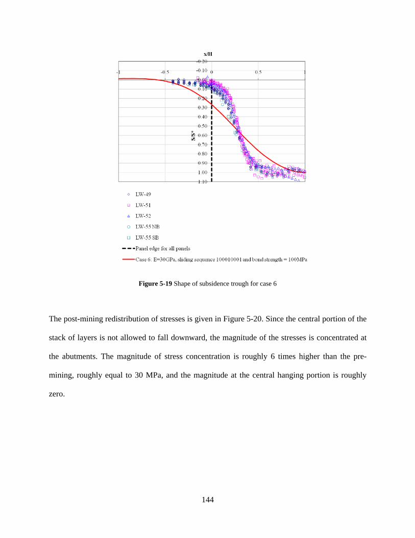
144
Figure 5-19 Shape of subsidence trough for case 6
The post-mining redistribution of stresses is given in Figure 5-20. Since the central portion of the
stack of layers is not allowed to fall downward, the magnitude of the stresses is concentrated at
the abutments. The magnitude of stress concentration is roughly 6 times higher than the pre-
mining, roughly equal to 30 MPa, and the magnitude at the central hanging portion is roughly
zero.

145
Figure 5-20 Post-mining vertical stress redistribution for case 6
5.1.2.7 Case 7
In case 7, tuning of the Young's modulus was done in order to improve the S*/M to approach the
one measured in the field roughly equal to 0.7. The modulus was set equal to 23 GPa. All other
features are those of case 6, including the sliding sequence of 100010001. This seventh model is
given in Figure 5-21. S*/M in this model turns out to be equal to 0.7 as the whole stack of layers
does not touch the floor. The readings of subsidence were corrected by subtracting the initial
settlement due to the application of gravity to the whole model. The shape is reasonably good as
in the previous case and the stresses have the same limitations as in the previous model.
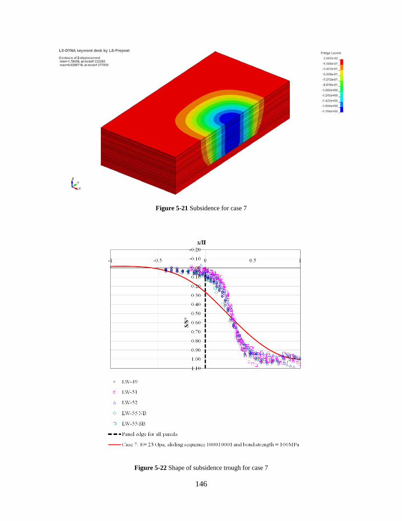
146
Figure 5-21 Subsidence for case 7
Figure 5-22 Shape of subsidence trough for case 7

147
Figure 5-23 Post-mining vertical stress redistribution for case 7
5.1.3 The effect of horizontal in-situ stresses
Horizontal in-situ stresses can be extremely high in southwestern Pennsylvania, in cases reaching
a ratio of 5:1 when compared to vertical stresses as illustrated in Figure 5-24 (Mark and Gadde
2008), where the circled data points correspond to eastern United States cases. A model with the
properties contained in Table 5-2 is given in Figure 5-25. Figure 5-26 and Figure 5-27 provide
details of the influence of the large horizontal pressure. The thin layers tend to warp, thus
exerting a lifting effect that keeps the upper layers from freely falling downward. The subsidence
factor obtained with this model was 0.83, and the vertical stress distribution and trough shape are
given in Figure 5-28 and Figure 5-29, respectively.

148
Table 5-2 Mechanical properties of model considering horizontal stresses
Shear Modulus, G [GPa] 4.6
Density [kg/m3] 2650
Yield stress, σy [MPa] 28
Plastic stiffness, Ep [MPa] 0.1
Bulk Modulus, K [GPa] 7.7
Young's Modulus, E [GPa] 11.5
Figure 5-24 Horizontal in-situ stress database (Mark and Gadde 2008)

149
Figure 5-25 Subsidence considering the effect of horizontal in-situ stresses
Figure 5-26 View of post-mining gaps between layers and deformed surface

150
Figure 5-27 Detail of warped layers and gaps created due to high in-situ stress

151
Figure 5-28 Vertical stresses at the end of extraction
Figure 5-29 Normalized subsidence profile
5.1.4 Results including a highway embankment
For the general visualization of embankment behavior, a model with the properties shown in
Table 5-3 and Table 5-4 was developed. Figure 5-30 shows that subsidence or vertical
deformation is essentially independent of the presence of the embankment. This has been known
to the subsidence community in that vertical deformations are not sensitive to hilly conditions.
This fact also made it possible to develop the empirical model described in chapter 4.0 . On the

152
other hand, horizontal deformations are very sensitive to the irregular shape of the highway
embankment, and the asymmetry in horizontal deformation distribution is evident in Figure 5-31.
Figure 5-32 shows two lines along which subsidence and horizontal deformations were
calculated. The results are given in Figure 5-33 and Figure 5-34 and they demonstrate that under
the special conditions of highway embankments, the general assumption that trough slope and
horizontal deformation are linearly correlated, is not generally valid. Even though the
embankment underwent a less steep deformation, the horizontal deformation was substantially
higher than on the overburden. This would naturally be based on the fact that the overburden is
formed by strong, confined rock, whereas the embankment is weaker, formed by compacted
soils, and unconfined. Figure 5-34 also illustrates the asymmetry in the distribution of horizontal
deformation as a consequence of the asymmetry in the embankment mass distribution. This
finding is even clearer from the real data, as depicted for example in Figure 3-23 or Figure 3-25.
Table 5-3 Mechanical properties of model overburden
Shear Modulus, G [GPa] 9.4
Density [kg/m3] 2650
Yield stress, σy [MPa] 38
Plastic stiffness, Ep [MPa] 0.1
Bulk Modulus, K [GPa] 13.7
Young's Modulus, E [GPa] 23
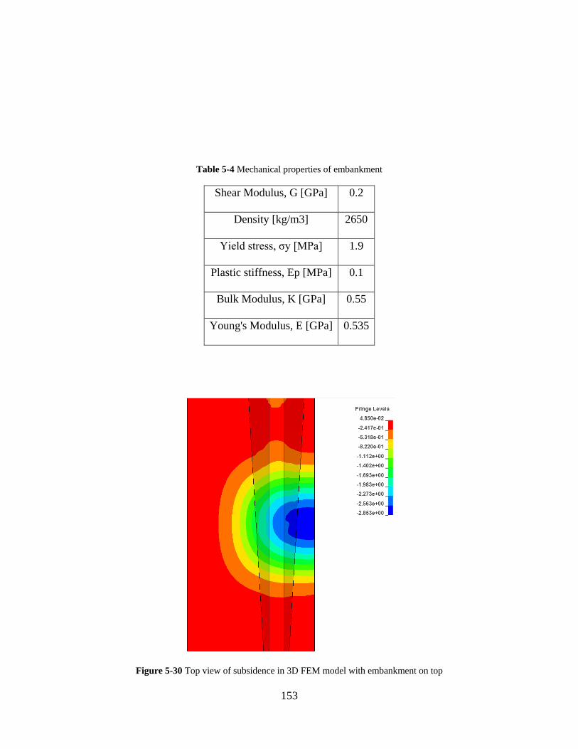
153
Table 5-4 Mechanical properties of embankment
Shear Modulus, G [GPa] 0.2
Density [kg/m3] 2650
Yield stress, σy [MPa] 1.9
Plastic stiffness, Ep [MPa] 0.1
Bulk Modulus, K [GPa] 0.55
Young's Modulus, E [GPa] 0.535
Figure 5-30 Top view of subsidence in 3D FEM model with embankment on top

154
Figure 5-31 Lateral deformation distribution
Figure 5-32 Profile lines on embankment and terrain for horizontal deformation

155
Figure 5-33 Subsidence profiles along embankment and virgin ground lines
Figure 5-34 Horizontal deformation along embankment and virgin ground lines

156
6.0 CONCLUSIONS
From the development of the new subsidence model described in this work, four general conclusions may
be drawn.
First, a clear relationship has been shown to exist between the subsidence factor, S*/M, and the
overburden thickness, H, whereby the subsidence factor decreases with overburden thickness. This
variation exists for values of the width-to-depth ratio, W/H, that are well above the critical threshold of
1.2. This means that, even for supercritical cases, the subsidence factor of a specific region may still vary
as different mining depths are considered. It is important to note that this contradicts a common notion
that the subsidence factor in a given region approaches a constant value for W/H > 1.2.
Second, an extension of the so called profile functions has been presented for three dimensions,
for which in the past influence functions have been employed. The influence function is more restricted.
For instance, a profile can be too sharp to be described by influence functions.
Third, a simultaneous description of the so called static and dynamic subsidence was made
through the methodology described. This was possible because the data were both spatially and
temporally considered. This is useful in that a complete final and in-progress description of the
subsidence trough can be made in three dimensions in a single model.
Fourth, the use of mathematical functions made it possible to derive the subsidence information
indices. Moreover, the function, as shown, applies to both symmetric and asymmetric subsidence profiles.
From the development of the numerical subsidence model described in this work, four general
conclusions may be drawn.

157
First, in order for a FEM model to correctly simulate the complete mechanism associated to mine
subsidence, fracturing of the material would need to be implemented. This would be the most direct way
to reproduce the so-called bulking factor that has a remarkable influence on the subsidence factor. Since
this is impractical due to the extremely expensive computational cost, some conditions need to be
imposed, such as the remaining elements on the floor that account for the bulking factor in an indirect
way.
Second, the horizontal in-situ stresses seem to play a role on the subsidence factor, especially
when they are very high. These stresses seem to be particularly high in this region of the world, where the
typical subsidence factors also happen to be very low. Obviously, without a sound modeling of the
fracturing of the rock and its consequent bulking, it is very difficult to draw conclusions on the
importance of the role of in-situ stresses on subsidence. Nevertheless, the observed results would suggest
that there is a connection between in-situ stresses and subsidence magnitudes.
Third, the behavior of horizontal deformations of earthen structures was demonstrated through a
simple example. This quick result is in good agreement with observations and unfortunately suggests that
the use of current empirical subsidence tools to predict lateral deformations would be extremely
unreliable when applied to embankments or earth dams. In such cases, detailed numerical models should
be encouraged.
Fourth, the FEM developed here brought the important results obtained in the past in 2D to a
sound 3D version that serves as an excellent platform for further research. Beyond the case of
embankments, any structure could be modeled in a flexible way.

158
BIBLIOGRAPHY
1. Agioutantis, Z. and M. Karmis (2009). Surface Deformation Prediction System for Windows Virginia Polytechnic Institute and State University.
2. Agioutantis, Z., M. Karmis, et al. (1987). Prediction of surface subsidence and strain in the Appalachian coalfields using numerical methods. 7th International Conference on Ground Control in Mining, Morgantown, WV, USA, West Virginia University.
3. Alejano, L. R., P. Ramírez-Oyanguren, et al. (1999). "FDM predictive methodology for subsidence due to flat and inclined coal seam mining." International Journal of Rock Mechanics and Mining Sciences 36(4): 475-491.
4. Coulthard, M. A. and A. J. Dutton (1988). Numerical modelling of subsidence induced by underground coal mining. The 29th U.S. Symposium on Rock Mechanics (USRMS). Minneapolis, MN, A. A. Balkema, Rotterdam. Permission to Distribute - American Rock Mechanics Association.
5. Earth (2006). S.R. 0079 Longwall Mining Emerald Mine Panel B-4 Greene County, PA. Harrisburg, Pennsylvania, USA, Pennsylvania Department of Transportation.
6. Edmunds, W. E. (1999). Chapter 11: Pennsylvanian-Permian Transition and Permian. Geology of Pennsylvania. C. H. Schultz. Harrisburg, Pittsburgh, Pennsylvania Geological Survey Pittsburgh Geological Society: 171-177.
7. Edmunds, W. E., V. W. Skema, et al. (1999). Chapter 10: Pennsylvanian. Geology of Pennsylvania. C. H. Schultz. Harrisburg, Pittsburgh, Pennsylvania Geological Survey Pittsburgh Geological Society: 156.
8. GeoTDR (2001). Effects of undermining Interstate Route 70, South Strabane Township, Washington County, Pennsylvania. Westerville, Ohio, USA.
9. Graybill, F. A. and H. K. Iyer (1994). Regression Analysis: Concepts and Applications. Belmont, California, USA, Dusbury Press An Imprint of Wadsworth Publishing Company.
10. Gutiérrez, J. J., L. E. Vallejo, et al. (2010). A study of highway subsidence due to longwall mining using data collected from I-79. Pittsburgh, Pennsylvania, Pennsylvania Department of Transportation: 402.

159
11. Heasley, K. A. and T. M. Barton (1998). Subsidence Prediction Using a Laminated, Boundary-Element Program. 3rd North American Rock Mechanics Symposium. Cancun, Mexico: 381-390.
12. Jarosz, A., M. Karmis, et al. (1990). "Subsidence development with time - experiences from longwall operations in the Appalachian coalfield." International Journal of Mining and Geological Engineering: 261-273.
13. Jeran, P. and V. Adamek (1988). Subsidence due to undermining of sloping terrain: A case study. Report of Investigations, United States Department of Interior Bureau of Mines.
14. Karmis, M. (1987). Prediction of ground movements due to underground mining in the Eastern United States coalfields. Blacksburg, VA, USA, Virginia Polytechnic Institute and State University.
15. Karmis, M., Z. Agioutantis, et al. (2008). Enhancing mine subsidence prediction and control methodologies. 27th International Conference on Ground Control in Mining, Morgantown, WV, USA, West Virginia University.
16. Karmis, M., C. Haycocks, et al. (1992). The prediction of ground movement caused by mining. 3rd Subsidence Workshop Due to Underground Mining, Morgantown, WV, USA, West Virginia University.
17. Karmis, M., T. Triplett, et al. (1983). Mining Subsidence And Its Prediction In The Appalachian Coalfield. The 24th U.S. Symposium on Rock Mechanics (USRMS). College Station, TX, The Association of Engineering Geologists. Permission to Distribute - American Rock Mechanics Association.
18. Kratzsch, H. (1983). Mining Subsidence Engineering. Berlin Heidelberg New York, Springer-Verlag.
19. Kratzsch, H. (2008). Bergschadenkunde. Bochum, Deutscher Markscheider-Verein e.V.
20. Luo, Y. and S. S. Peng (1999). "Integrated approach for predicting mining subsidence in hilly terrain." Mining Engineering: 100-104.
21. Luo, Y., S. S. Peng, et al. (1996). Identification of factors affecting horizontal displacement in subsidence process. 15th International Conference on Ground Control in Mining, Golden, CO, USA.
22. Mark, C. and M. Gadde (2008). Global Trends in Coal Mine Horizontal Stress Measurements. 27th International Conference on Ground Control in Mining, Morgantown, WV, West Virginia University.
23. Mine Subsidence Engineering Consultants (2007). "Introduction to longwall mining and subsidence." Retrieved 08/19/2009, 2009, from www.minesubsidence.com.

160
24. Mohammad, N., P. W. Lloyd, et al. (1997). Longwall surface subsidence prediction through numerical modeling. 16th International Conference on Ground Control in Mining, Morgantown, WV, USA, West Virginia University.
25. Morsy, K. and S. S. Peng (2002). Numerical modeling of the gob loading mechanism in longwall coal mines. 21st International Conference on Ground Control in Mining, Morgantown, WV, West Virginia University.
26. NCB (1975). Subsidence Engineer's Handbook, National Coal Board.
27. OSMRE (1986). Guidance manual on subsidence control, United States Department of Interior.
28. Oyler, D., C. Mark, et al. (2004). Performance of roof support under high stress in a U.S. coal mine, NIOSH.
29. Peng, S. S. (1992). Surface Subsidence Engineering. Littleton, CO, USA, Society for Mining, Metallurgy, and Exploration, Inc.
30. Peng, S. S. (2008). Coal Mine Ground Control. Morgantown, WV, Department of Mining Engineering, College of Engineering and Mineral Resources, West Virginia University.
31. Peng, S. S. and H. S. Chiang (1984). Longwall Mining. New York, John Wiley & Sons.
32. Stone, R. W. (1932). Geology and mineral resources of Greene County Pennsylvania. Harrisburg, Pennsylvania, USA, Pennsylvania Geological Survey.
33. Su, D. (1991). Finite element modeling of subsidence induced by underground coal mining: The influence of material nonlinearity and shearing along existing planes of weakness. 10th International Conference on Ground Control in Mining, Morgantown, WV, USA, West Virginia University.
34. Szostak-Chrzanowski, A. (1988). An iterative modeling of ground subsidence using non-linear elastic finite element analysis. 5th International Symposium on Deformation Measurements, Fredericton, N.B., University of New Brunswick.
35. Tajdus, K. (2009). "New method for determining the elastic parameters of rock mass layers in the region of underground mining influence." International Journal of Rock Mechanics and Mining Sciences 46(8): 1296-1305.
36. VPI&SU (1987). Prediction of ground movements due to underground mining in the Eastern United States coalfields. Blacksburg, VA, USA, Virginia Polytechnic Institute and State University: 205.
37. Whittaker, B. N. and D. J. Reddish (1989). Subsidence: Occurrence, Prediction, and Control, Elsevier Science Publisher B.V.