metaheuristics in water, geotechnical and transport engineering || optimization and metaheuristic...

1 Optimization and MetaheuristicAlgorithms in Engineering

Xin-She Yang

Centre for Mathematics and Scientific Computing, National PhysicalLaboratory, Teddington, UK

1.1 Introduction

Optimization is everywhere, and thus it is an important paradigm with a wide range

of applications. In almost all applications in engineering and industry, we are trying

to optimize something—whether to minimize the cost and energy consumption or

to maximize profit, output, performance, and efficiency. In reality, resources, time,

and money are always limited; consequently, optimization is far more important in

practice (Yang, 2010b; Yang and Koziel, 2011). The optimal use of available

resources of any sort requires a paradigm shift in scientific thinking because most

real-world applications have far more complicated factors and parameters to affect

how the system behaves.

Contemporary engineering design is heavily based on computer simulations,

which introduces additional difficulties to optimization. Growing demand for

accuracy and ever-increasing complexity of structures and systems results in the

simulation process being more and more time consuming. In many engineering

fields, the evaluation of a single design can take as long as several days or even

weeks. Any method that can speed up the simulation time and optimization pro-

cess can thus save time and money.

For any optimization problem, the integrated components of the optimization

process are the optimization algorithm, an efficient numerical simulator, and a real-

istic representation of the physical processes that we wish to model and optimize.

This is often a time-consuming process, and in many cases, the computational costs

are usually very high. Once we have a good model, the overall computation costs

are determined by the optimization algorithms used for searching and the numerical

solver used for simulation.

Search algorithms are the tools and techniques used to achieve optimality of the

problem of interest. This search for optimality is complicated further by the fact

that uncertainty is almost always present in the real world. Therefore, we seek not

only the optimal design but also the robust design in engineering and industry.

Metaheuristics in Water, Geotechnical and Transport Engineering. DOI: http://dx.doi.org/10.1016/B978-0-12-398296-4.00001-5

© 2013 Elsevier Inc. All rights reserved.

http://dx.doi.org/10.1016/B978-0-12-398296-4.00001-5

Optimal solutions, which are not robust enough, are not practical in reality.

Suboptimal solutions or good robust solutions are often the choice in such cases.

Simulations are often the most time-consuming part. In many applications,

an optimization process often involves evaluating objective function many times

(with often thousands, hundreds of thousands, and even millions of configurations).

Such evaluations often involve the use of extensive computational tools such as

a computational fluid dynamics simulator or a finite element solver. Therefore, effi-

cient optimization with an efficient solver is extremely important.

Optimization problems can be formulated in many ways. For example, the com-

monly used method of least squares is a special case of maximum-likelihood

formulations. By far, the best-known formulation is to write a nonlinear optimiza-

tion problem as

minimize fiðxÞ; i5 1; 2; . . . ; M ð1:1Þ

subject to the constraints

hjðxÞ5 0; j5 1; 2; . . . ; J ð1:2Þ

and

gkðxÞ# 0; k5 1; 2; . . . ; K ð1:3Þ

where fi, hj, and gk are general nonlinear functions. Here, the design vector

x5 (x1,x2,. . ., xn) can be continuous, discrete, or mixed in n-dimensional space.

The functions fi are called objective or cost functions, and when M. 1, the

optimization is multiobjective or multicriteria (Sawaragi et al., 1985; Yang,

2010b). It is possible to combine different objectives into a single objective,

though multiobjective optimization can give far more information and insight

into the problem. It is worth pointing out here that we write the problem as a

minimization problem, but it can also be written as a maximization by simply

replacing fi(x) by 2fi(x).

When all functions are nonlinear, we are dealing with nonlinear constrained

problems. In some special cases when fi, hj, gk are linear, the problem becomes

linear, and we can use widely linear programming techniques such as the simplex

method. When some design variables can take only discrete values (often integers),

while other variables are real and continuous, the problem is of mixed type,

which is often difficult to solve, especially for large-scale optimization.

A very special class of optimization is the convex optimization, which has

guaranteed global optimality. Any optimal solution is also the global optimum,

and most importantly, there are efficient algorithms of polynomial time to solve

such problems (Conn et al., 2009). These efficient algorithms, such as the inte-

rior-point methods (Karmarkar, 1984), are widely used and have been implemen-

ted in many software packages.

2 Metaheuristics in Water, Geotechnical and Transport Engineering

1.2 Three Issues in Optimization

There are three main issues in the simulation-driven optimization and modeling,

and they are the efficiency of an algorithm, the efficiency and accuracy of a

numerical simulator, and the assignment of the right algorithms to the right prob-

lem. Despite their importance, there are no satisfactory rules or guidelines for such

issues. Obviously, we try to use the most efficient algorithms available, but the

actual efficiency of an algorithm depends on many factors such as the inner work-

ing of an algorithm, the information needed (such as objective functions and their

derivatives), and implementation details. The efficiency of a solver is even more

complicated, depending on the actual numerical methods used and the complexity

of the problem of interest. As for choosing the right algorithms for the right

problems, there are many empirical observations, but no agreed guidelines. In fact,

there is no universally efficient algorithms for all types of problems. Therefore,

the choice depends on many factors and is sometimes subject to the personal

preferences of researchers and decision makers.

1.2.1 Efficiency of an Algorithm

An efficient optimizer is very important to ensure the optimal solutions are reach-

able. The essence of an optimizer is a search or optimization algorithm implemen-

ted correctly so as to carry out the desired search (though not necessarily

efficient). It can be integrated and linked with other modeling components. There

are many optimization algorithms in the literature, and no single algorithm is

suitable for all problems, as dictated by the No Free Lunch Theorems (Wolpert

and Macready, 1997).

Optimization algorithms can be classified in many ways, depending on the focus

or the characteristics that we are trying to compare. Algorithms can be classified as

gradient-based (or derivative-based) and gradient-free (or derivative-free). The clas-

sic methods of steepest descent and the Gauss�Newton methods are gradient based,

as they use the derivative information in the algorithm, while the Nelder�Mead

downhill simplex method (Nelder and Mead, 1965) is a derivative-free method

because it uses only the values of the objective, not any derivatives.

Algorithms can also be classified as deterministic or stochastic. If an algorithm

works in a mechanically deterministic manner without any random nature, it is

called deterministic. For such an algorithm, it will reach the same final solution

if we start with the same initial point. The hill-climbing and downhill simplex

methods are good examples of deterministic algorithms. On the other hand, if

there is some randomness in the algorithm, the algorithm will usually reach a dif-

ferent point every time it is run, even starting with the same initial point.

Genetic algorithms and hill climbing with a random restart are good examples of

stochastic algorithms.

Analyzing stochastic algorithms in more detail, we can single out the type of

randomness that a particular algorithm is employing. For example, the simplest

3Optimization and Metaheuristic Algorithms in Engineering

and yet often very efficient method is to introduce a random starting point for a

deterministic algorithm. The well-known hill-climbing method with random restart

is a good example. This simple strategy is both efficient in most cases and easy to

implement in practice. A more elaborate way to introduce randomness to an algo-

rithm is to use randomness inside different components of an algorithm, and in

this case, we often call such algorithm heuristic or, more often, metaheuristic

(Talbi, 2009; Yang, 2008, 2010b). A very good example is the popular genetic

algorithms, which use randomness for crossover and mutation in terms of a cross-

over probability and a mutation rate. Here, heuristic means to search by trial and

error, while metaheuristic is a higher level of heuristics. However, modern litera-

ture tends to refer to all new stochastic algorithms as metaheuristic. In this book,

we will use metaheuristic to mean either. It is worth pointing out that metaheuris-

tic algorithms are a hot research topic, and new algorithms appear almost yearly

(Yang, 2008, 2010b).

From the mobility point of view, algorithms can be classified as local or global.

Local search algorithms typically converge toward a local optimum, not necessar-

ily (often not) the global optimum, and such algorithms are often deterministic

and have no ability of escaping local optima. Simple hill climbing is an example.

On the other hand, we always try to find the global optimum for a given problem,

and if this global optimality is robust, it is often the best, though it is not always

possible to find such global optimality. For global optimization, local search algo-

rithms are not suitable. We have to use a global search algorithm. Modern meta-

heuristic algorithms in most cases are intended for global optimization, though the

process is not always successful or efficient. A simple strategy such as hill climb-

ing with random restart may change a local search algorithm into a global search.

In essence, randomization is an efficient component for global search algorithms.

In this chapter, we will provide a brief review of most metaheuristic optimization

algorithms.

Straightforward optimization of a given objective function is not always practi-

cal. In particular, if the objective function comes from a computer simulation,

it may be computationally expensive, noisy, or nondifferentiable. In such cases,

so-called surrogate-based optimization algorithms may be useful where the direct

optimization of the function of interest is replaced by iterative updating and reop-

timization of its model—i.e., a surrogate. The surrogate model is typically con-

structed from the sampled data of the original objective function; however, it is

supposed to be cheap, smooth, easy to optimize, and yet reasonably accurate so

that it can produce a good prediction of the function’s optimum. Multifidelity or

variable-fidelity optimization is a special case of surrogate-based optimization,

where the surrogate is constructed from the low-fidelity model (or models) of the

system of interest (Koziel and Yang, 2011). Using variable-fidelity optimization

is particularly useful, as the reduction of the computational cost of the optimiza-

tion process is of primary importance.

Whatever the classification of an algorithm is, we have to make the right choice

to use an algorithm correctly, and sometimes using a proper combination of algo-

rithms may achieve far better results.


1.2.2 The Right Algorithms?

From the optimization point of view, the choice of the right optimizer or algo-

rithm for a given problem is crucially important. The algorithm chosen for an

optimization task will largely depend on the type of the problem, the nature of an

algorithm, the desired quality of solutions, the available computing resource, time

limit, availability of the algorithm implementation, and the expertise of the deci-

sion makers (Yang, 2010b; Yang and Koziel, 2011).

The nature of an algorithm often determines if it is suitable for a particular type

of problem. For example, gradient-based algorithms such as hill climbing are not

suitable for an optimization problem with a discontinuous objective. Conversely,

the type of problem we are trying to solve also determines the algorithms we may

choose. If the objective function of an optimization problem at hand is highly non-

linear and multimodal, classic algorithms such as hill climbing and downhill sim-

plex are not suitable, as they are local search algorithms. In this case, global

optimizers, such as particle swarm optimization and cuckoo search, are most

suitable (Yang, 2010a; Yang and Deb, 2010).

Obviously, the choice is also affected by the desired solution quality and avail-

able computing resources. Because computing resources are limited in most appli-

cations, we have to obtain good solutions (if not necessary the best) in a reasonable

and practical time. Therefore, we have to balance resource availability with solution

quality. We cannot achieve solutions with guaranteed quality, though we strive to

obtain the best-quality solutions that we possibly can. If time is the main constraint,

we can use some greedy methods, or hill climbing with a few random restarts.

Sometimes, even with the best possible intentions, the availability of an algo-

rithm and the expertise of the decision makers are the ultimate defining factors for

choosing an algorithm. Even though some algorithms are better for the given prob-

lem at hand, we may not have that algorithm implemented in our system or we do

not have such access, which limits our choice. For example, Newton’s method,

hill-climbing, Nelder�Mead downhill simplex, trust-region methods (Conn et al.,

2009), and interior-point methods are implemented in many software packages,

which may also increase their popularity in applications. In practice, even with the

best possible algorithms and well-crafted implementation, we still may fail to get

the desired solutions. This is the nature of nonlinear global optimization, as most of

such problems are Non-deterministic polynomial-time hard (NP-hard), and no effi-

cient (in the polynomial sense) solutions exist for a given problem. Thus, the chal-

lenges of research in computational optimization and applications are to find the

right algorithms most suitable for a given problem so as to obtain good solutions

(perhaps also the best solutions globally), in a reasonable timescale with a limited

amount of resources. We aim to do this in an efficient, optimal way.

1.2.3 Efficiency of a Numerical Solver

To solve an optimization problem, the most computationally extensive part is prob-

ably the evaluation of the design objective to see if a proposed solution is feasible


and/or if it is optimal. Typically, we have to carry out these evaluations many

times, often thousands, hundreds of thousands, and even millions of times (Yang,

2008, 2010b). Things become even more challenging computationally, when each

evaluation task takes a long time to complete using some black-box simulators.

If this simulator is a finite element or computational fluid dynamics solver, the run-

ning time of each evaluation can take from a few minutes to a few hours or even

weeks. Therefore, any approach to save computational time either by reducing the

number of evaluations or by increasing the simulator’s efficiency will save time

and money. In general, a simulator can be a simple function subroutine, a multi-

physics solver, or an external black-box evaluator.

The main way to reduce the number of objective evaluations is to use an effi-

cient algorithm, so that only a small number of such evaluations are needed. In

most cases, this is not possible. We have to use some approximation techniques to

estimate the objectives, or to construct an approximation model to predict the sol-

ver’s outputs without actually using the solver. Another way is to replace the origi-

nal objective function by its lower-fidelity model, e.g., obtained from a computer

simulation based on coarsely discretized structure of interest. The low-fidelity

model is faster, but not as accurate as the original one, and therefore it has to be

corrected. Special techniques have to be applied to use an approximation or cor-

rected low-fidelity model in the optimization process so that the optimal design can

be obtained at a low computational cost (Koziel and Yang, 2011).

1.3 Metaheuristics

Metaheuristic algorithms are often nature-inspired, and they are now among the

most widely used algorithms for optimization. They have many advantages over

conventional algorithms, as we can see from many case studies presented in later

chapters in this book. There are a few recent books that are solely dedicated to

metaheuristic algorithms (Talbi, 2009; Yang, 2008, 2010a,b). Metaheuristic algo-

rithms are very diverse, including genetic algorithms, simulated annealing, differ-

ential evolution (DE), ant and bee algorithms, particle swarm optimization,

harmony search, firefly algorithm, cuckoo search, and others. Here, we will intro-

duce some of these algorithms briefly.

1.3.1 Ant Algorithms

Ant algorithms, especially the ant colony optimization (Dorigo and Stutle, 2004),

mimic the foraging behavior of social ants. Primarily, ants use pheromones as a

chemical messenger, and the pheromone concentration can also be considered as

the indicator of quality solutions to a problem of interest. As the solution is often

linked with the pheromone concentration, the search algorithms often produce

routes and paths marked by the higher pheromone concentrations, and therefore,

ant-based algorithms are particularly suitable for discrete optimization problems.


The movement of an ant is controlled by pheromones that will evaporate over

time. Without such time-dependent evaporation, ant algorithms will lead to prema-

ture convergence to the (often wrong) solutions. With proper pheromone evapora-

tion, they usually behave very well.

There are two important issues here: the probability of choosing a route and the

evaporation rate of the pheromones. There are a few ways of solving these pro-

blems, although this is still an area of active research. For a network routing prob-

lem, the probability of ants at a particular node i to choose the route from node i to

node j is given by

pij 5φαijd

βijPn

i;j51 φαijd

βij

ð1:4Þ

where α. 0 and β. 0 are the influence parameters, and their typical values are

α � β � 2. Here, φij is the pheromone concentration on the route between i and j

and dij, the desirability of the same route. Some a priori knowledge about the

route, such as the distance sij, is often used so that dij~1/sij, which implies that

shorter routes will be selected due to their shorter traveling time; and thus the

pheromone concentrations on these routes are higher. This is because the traveling

time is shorter, and thus the less amount of the pheromone has been evaporated

during this period.

1.3.2 Bee Algorithms

Bee-inspired algorithms are more diverse—a few use pheromones, but most do not.

Almost all bee algorithms are inspired by the foraging behavior of honeybees in

nature. Interesting characteristics, such as waggle dancing, polarization, and nectar

maximization, are often used to simulate the allocation of the foraging bees along

flower patches, and thus in different regions of the search space. For a more com-

prehensive review, see Yang (2010a) and Parpinelli and Lope (2011).

Different variants of bee algorithms use slightly different characteristics of the

behavior of bees. For example, in the honeybee-based algorithms, forager bees are

allocated to different food sources (or flower patches) so as to maximize the total

nectar intake (Karaboga, 2005; Nakrani and Tovey, 2004; Pham et al., 2006; Yang,

2005). In the virtual bee algorithm (VBA), pheromone concentrations can be linked

with the objective functions more directly (Yang, 2005). The artificial bee colony

(ABC) optimization algorithm was first developed by Karaboga (2005). In the

ABC algorithm, the bees in a colony are divided into three groups: employed bees

(forager bees), onlooker bees (observer bees), and scouts. Unlike the honeybee

algorithm, which has only two groups of bees (forager bees and observer bees),

bees in ABC are more specialized (Afshar et al., 2007; Karaboga, 2005).

Similar to the ant-based algorithms, bee algorithms are very flexible in dealing

with discrete optimization problems. Combinatorial optimization, such as routing

and optimal paths, has been solved by ant and bee algorithms. In principle, they


can solve both continuous optimization and discrete optimization problems; how-

ever, they should not be the first choice for continuous problems.

1.3.3 The Bat Algorithm

The bat algorithm is a relatively new metaheuristic (Yang, 2010c). Microbats use a

type of sonar called echolocation to detect prey, avoid obstacles, and locate their

roosting crevices in the dark, and the bat algorithm was inspired by this echoloca-

tion behavior. These bats emit a very loud sound pulse and listen for the echo that

bounces back from the surrounding objects. Their pulses vary in properties and can

be correlated with their hunting strategies, depending on the species. Most bats use

short, frequency-modulated signals to sweep through about an octave, while others

more often use constant-frequency signals for echolocation. Their signal bandwidth

varies depending on the species and often increased by using more harmonics.

The bat algorithm uses three idealized rules: (1) all bats use echolocation to

sense distance, and they also “know” the difference between food/prey and

background barriers in some unknown way; (2) a bat flies randomly with a velocity

vi at position xi with a fixed frequency range [fmin, fmax], varying its emission rate

rA[0,1] and loudness A0 to search for prey, depending on the proximity of their tar-

get; (3) although the loudness can vary in many ways, we assume that it varies

from a large (positive) A0 to a minimum constant value Amin. These rules can be

translated into the following formulas:

fi 5 fmin1 ðfmax 2 fminÞε; vt11i 5 vti 1ðxti 2 x�Þfi; xt11

i 5 xti 1 vti ð1:5Þ

where ε is a random number drawn from a uniform distribution and x� is the cur-

rent best solution found so far during iterations. The loudness and pulse rate can

vary with iteration t in the following way:

At11i 5αAt

i; rti 5 r0i ½12 expð2βtÞ� ð1:6Þ

Here, α and β are constants. In fact, α is similar to the cooling factor of a cooling

schedule in the simulated annealing, which will be discussed next. In the simplest

case, we can use α5β, and we have, in fact, used α5β5 0.9 in most simulations.

The bat algorithm has been extended to the multiobjective bat algorithm

(MOBA) by Yang (2011a), and preliminary results suggested that it is very effi-

cient (Yang and Gandomi, 2012).

1.3.4 Simulated Annealing

Simulated annealing is among the first metaheuristic algorithms (Kirkpatrick et al.,

1983). It was essentially an extension of the traditional Metropolis�Hastings algo-

rithm but applied in a different context. The basic idea of the simulated annealing


algorithm is to use random search in terms of a Markov chain, which not only

accepts changes that improve the objective function but also keeps some changes

that are not ideal.

In a minimization problem, for example, any better moves or changes that

decrease the value of the objective function f will be accepted; however, some

changes that increase f will also be accepted with a probability P. This probability

P, also called the transition probability, is determined by

P5 exp 2ΔE

kBT

� �ð1:7Þ

where kB is Boltzmann’s constant, T is the temperature for controlling the anneal-

ing process, and ΔE is the change of the energy level. This transition probability is

based on the Boltzmann distribution in statistical mechanics.

The simplest way to link ΔE with the change of the objective function Δf is to

use ΔE5 γΔf, where γ is a real constant. For simplicity without losing generality,

we can use kB5 1 and γ5 1. Thus, the probability P simply becomes

PðΔf ; TÞ5 e2Δf=T ð1:8Þ

Whether or not a change is accepted, a random number r is often used as a

threshold. Thus, if P. r, the move is accepted.

Here, the choice of the right initial temperature is crucial. For a given change

Δf, if T is too high (T!N), then P!1, which means almost all the changes will

be accepted. If T is too low (T!0), then any Δf. 0 (worse solutions) will rarely

be accepted as P!0, and thus the diversity of the solution is limited, but any

improvement Δf will almost always be accepted. In fact, the special case T!0 cor-

responds to the classical hill-climbing method because only better solutions are

accepted, and the system is essentially climbing or descending a hill. So, a proper

temperature range is very important.

Another important issue is how to control the annealing or cooling process so

that the system cools gradually from a higher temperature, ultimately freezing to a

global minimum state. There are many ways of controlling the cooling rate or the

decrease of the temperature. Geometric cooling schedules are often widely used,

which essentially decrease the temperature by a cooling factor 0,α, 1, so that T

is replaced by αT or

TðtÞ5 T0αt; t5 1; 2; . . . ; tf ð1:9Þ

where tf is the maximum number of iterations. The advantage of this method is that

T!0 when t!N, and thus, there is no need to specify the maximum number of

iterations if a tolerance or accuracy is prescribed.


1.3.5 Genetic Algorithms

Genetic algorithms are a class of algorithms based on the abstraction of Darwin’s

evolution of biological systems, pioneered by Holland and his collaborators in the

1960s and 1970s (Holland, 1975). Holland was probably the first to use genetic

operators such as the crossover and recombination, mutation, and selection in the

study of adaptive and artificial systems. Three main components or genetic operators

in genetic algorithms are crossover, mutation, and selection of the fittest. Each solu-

tion is encoded in a string (often binary or decimal) called chromosome.

The crossover of two parent strings produce offsprings (new solutions) by swapping

part or genes of the chromosomes. Crossover has a higher probability, typically

0.8�0.95. On the other hand, mutation is performed by flipping some digits of a

string, which generates new solutions. This mutation probability is typically low,

from 0.001 to 0.05. New solutions generated in each generation will be evaluated by

their fitness, which is linked to the objective function of the optimization problem.

The new solutions are selected according to their fitness—i.e., selection of the

fittest. Sometimes, to make sure that the best solutions remain in the population,

the best solutions are passed onto the next generation without much change,

a process called elitism.

Genetic algorithms have been applied to almost all areas of optimization, design,

and applications. There are hundreds of good books and thousands of research

articles. There are many variants and hybridization with other algorithms, and inter-

ested readers can refer to more advanced literature such as Goldberg (1989).

1.3.6 Differential Evolution

DE was developed by Storn and Price (Storn, 1996; Storn and Price, 1997). It is

a vector-based evolutionary algorithm that can be considered as a further development

in genetic algorithms. As with genetic algorithms, design parameters in a d-dimensional

search space are represented as vectors, and various genetic operators are operated over

their bits of strings. However, unlike genetic algorithms, DE carries out operations over

each component (or each dimension of the solution). Almost everything is done

in terms of vectors. For a d-dimensional optimization problem with d parameters, a

population of n solution vectors are initially generated, we have xi where i5 1,2,. . ., n.For each solution xi at any generation t, we use the conventional notation:

xti 5 ðxt1;i; xt2;i; . . . ; xtd;iÞ ð1:10Þ

which consists of d components in the d-dimensional space. This vector can be

considered as chromosomes or genomes.

DE consists of three main steps: mutation, crossover, and selection. Mutation is

carried out by the mutation scheme. For each vector xi at any time or generation t,

we first randomly choose three distinct vectors xp, xq, and xr at t, and then generate

a so-called donor vector by the mutation scheme

vt11i 5 xtp 1Fðxtq 2 xtrÞ ð1:11Þ


where FA[0,2] is a parameter, often referred to as the differential weight. This

requires that the minimum population size is n$ 4. In principle, FA[0,2], but in

practice, a scheme with FA[0,1] is more efficient and stable.

The crossover is controlled by a crossover probability CrA[0,1], and actual

crossover can be carried out in two ways: binomial and exponential. Selection is

essentially the same as that used in genetic algorithms. The goal is to select the fit-

test, and for the minimization problem, the minimum objective value. Therefore,

we have

xt11i 5

ut11i if f ðut11

i Þ# f ðxtiÞxti otherwise

�ð1:12Þ

Most studies have focused on the choice of F, Cr, and n, as well as the modifica-

tion of Eq. (1.11). In fact, when generating mutation vectors, we can use many

different ways of formulating Eq. (1.11), and this leads to various schemes with the

naming convention: DE/x/y/z, where x is the mutation scheme (rand or best), y is

the number of difference vectors, and z is the crossover scheme (binomial or expo-

nential). The basic DE/Rand/1/Bin scheme is given in Eq. (1.11). Following a simi-

lar strategy, we can design various schemes. In fact, more than 10 different

schemes have been formulated in the literature (Price et al., 2005).

1.3.7 Particle Swarm Optimization

Particle swarm optimization (PSO) was based on swarm behavior in nature,

such as fish and bird schooling (Kennedy and Eberhart, 1995). Since then, PSO

has generated much wider interest and forms an exciting, ever-expanding

research subject called swarm intelligence. This algorithm searches the space of

an objective function by adjusting the trajectories of individual agents, called par-

ticles, as the piecewise paths formed by positional vectors in a quasi-stochastic

manner.

The movement of a swarming particle consists of two major components: a sto-

chastic component and a deterministic component. Each particle is attracted to the

position of the current global best g� and its own best location x�i in history, while

at the same time, it has a tendency to move randomly. Let xi and vi be the position

vector and velocity for particle i, respectively. The new velocity vector is deter-

mined by the following formula:

vt11i 5 vti 1αε1 ½g� 2 xti�1βε2 ½x�i 2 xti� ð1:13Þ

where ε1 and ε2 are two random vectors, with each entry taking a value between 0

and 1. The Hadamard product of two matrices (u}v) is defined as the entrywise

product, i.e., [u}v]ij5 uijvij. The parameters α and β are the learning parameters

or acceleration constants, which can typically be taken as, for example, α � β � 2.


The initial locations of all particles should distribute relatively uniformly so that

they can sample over most regions, which is especially important for multimodal

problems. The initial velocity of a particle can be taken as zero, i.e., vt50i 5 0:

The new position can then be updated by

xt11i 5 xti 1 vt11

i ð1:14Þ

Although vi can be any value, it is usually located in some range [0, vmax].

There are many variants that extend the standard PSO algorithm (Kennedy

et al., 2001; Yang, 2008, 2010b), and the most noticeable improvement is probably

to use inertia function θ(t) so that vti is replaced by θðtÞvti:

vt11i 5 θvti 1αε1}½g� 2 xti�1 βε2}½x�i 2 xti� ð1:15Þ

where θ takes the value between 0 and 1. In the simplest case, the inertia function

can be taken as a constant, typically θ � 0.5 � 0.9. This is equivalent to introduc-

ing a virtual mass to stabilize the motion of the particles, and thus the algorithm is

expected to converge more quickly.

1.3.8 Harmony Search

Harmony search (HS) is a music-inspired algorithm (Geem et al., 2001), which can

be explained in more detail with the aid of the discussion of a musician’s improvi-

sation process. When a musician is improvising, he or she has three possible

choices: (1) play any famous piece of music (a series of pitches in harmony)

exactly from his or her memory; (2) play something similar to a known piece (thus

adjusting the pitch slightly); or (3) compose new or random notes. If we formalize

these three options for optimization, we have three corresponding components:

usage of harmony memory, pitch adjusting, and randomization.

The usage of harmony memory is important, as it is similar to choose the best-fit-

ting individuals in the genetic algorithms. This will ensure that the best harmonies

will be carried over to the new harmony memory. An important step is pitch adjust-

ment, which can be considered a local random walk. If xold is the current solution

(or pitch), then the new solution (pitch) xnew is generated by

xnew 5 xold 1 bpð2ε2 1Þ ð1:16Þ

where ε is a random number drawn from a uniform distribution [0,1]. Here, bp is

the bandwidth, which controls the local range of pitch adjustment. In fact, we can

see that the pitch adjustment (Eq. (1.16)) is a random walk.

Pitch adjustment is similar to the mutation operator in genetic algorithms.

Although adjusting pitch has a similar role, it is limited to certain local pitch

adjustment, and thus, it corresponds to a local search. The use of randomization


can drive the system further to explore various regions with high solution diversity

so as to find the global optimality.

1.3.9 Firefly Algorithm

The firefly algorithm (FA), first developed Yang (2008, 2009), was based on the

flashing patterns and behavior of fireflies. In essence, FA uses the following three

idealized rules:

1. Fireflies are unisexual, so one firefly will be attracted to other fireflies regardless of their

sex.

2. Their attractiveness is proportional to their brightness, and both decrease as their distance

increases. Thus, for any two flashing fireflies, the less brighter one will move toward the

brighter one. If a particular firefly does not find a brighter one, it will move randomly.

3. The brightness of a firefly is determined by the landscape of the objective function.

As a firefly’s attractiveness is proportional to the light intensity seen by adjacent

fireflies, we can now define the variation of attractiveness β with distance r by

β5β0 e2γr2 ð1:17Þ

where β0 is the attractiveness at r5 0.

The movement of a firefly i that is attracted to another more attractive (brighter)

firefly j is determined by

xt11i 5 xti 1β0e

2γr2ij ðxtj 2 xtiÞ1αεti ð1:18Þ

where the second term is based on the attraction. The third term is randomized,

with α being the randomization parameter and εti is a vector of random numbers

drawn from a Gaussian distribution or uniform distribution at time t. If β05 0, it

becomes a simple random walk. Furthermore, the randomization εti can easily be

extended to other distributions such as Levy flights.

The Levy flight essentially provides a random walk whose random step length is

drawn from a Levy distribution:

Lðs;λÞ5 s2ð11λÞ; 0,λ# 2 ð1:19Þ

which has an infinite variance with an infinite mean. Here the steps essentially form

a random walk process with a power-law step-length distribution with a heavy tail.

Some of the new solutions should be generated by a Levy walk around the best solu-

tion obtained so far, which will speed up the local search (Pavlyukevich, 2007).

A demo version of FA implementation, without Levy flights, can be found at

the Mathworks file exchange web site.1 FA has attracted much attention

1 http://www.mathworks.com/matlabcentral/fileexchange/29693-firefly-algorithm.


http://www.mathworks.com/matlabcentral/fileexchange/29809-cuckoo-search-cs-algorithm

(Apostolopoulos and Vlachos, 2011; Gandomi et al., 2011; Sayadi et al., 2010).

A discrete version of FA can efficiently solve NP-hard scheduling problems

(Sayadi et al., 2010), while a detailed analysis has demonstrated the efficiency of

FA over a wide range of test problems, including multiobjective load dispatch pro-

blems (Apostolopoulos and Vlachos, 2011). A chaos-enhanced FA with a basic

method for automatic parameter tuning has also been developed (Yang, 2011b).

1.3.10 Cuckoo Search

Cuckoo search (CS) is one of the latest nature-inspired metaheuristic algorithms

developed by Yang and Deb (2009). CS is based on the brood parasitism of some

cuckoo species. In addition, this algorithm is enhanced by the so-called Levy

flights (Pavlyukevich, 2007), rather than by simple isotropic random walks. Recent

studies show that CS is potentially far more efficient than the PSO and genetic

algorithms (Yang and Deb, 2010).

Cuckoos are fascinating birds, not only because of the beautiful sounds they can

make but also because of their aggressive reproduction strategy. Some species such

as the ani and Guira cuckoos lay their eggs in communal nests, though they may

remove others’ eggs to increase the hatching probability of their own. Quite a num-

ber of species engage in the obligate brood parasitism by laying their eggs in the

nests of other host birds (often other species).

For simplicity in describing the standard CS, we now use the following three

idealized rules:

1. Each cuckoo lays one egg at a time and dumps it in a randomly chosen nest.

2. The best nests with high-quality eggs will be carried over to the next generation.

3. The number of available host nests is fixed, and the probability that an egg laid by a

cuckoo is discovered by the host bird is paA[0,1]. In such a case, the host bird can either

get rid of the egg or abandon the nest and build a completely new nest.

As a further approximation, this last assumption can be approximated by stat-

ing that a fraction pa of the n host nests are replaced by new nests (with new

random solutions).

For a maximization problem, the quality or fitness of a solution can simply be

proportional to the value of the objective function. Other forms of fitness can be

defined in a similar way to the fitness function in genetic algorithms.

For the implementation point of view, we can use the following simple represen-

tations that each egg in a nest represents a solution, and each cuckoo can lay only

one egg (thus representing one solution), the aim being to use the new and poten-

tially better solutions (cuckoos) to replace less good solutions in the nests.

Obviously, this algorithm can be extended to the more complicated case, where

each nest has multiple eggs representing a set of solutions. For this discussion,

we will use the simplest approach, where each nest has only a single egg. In this

case, there is no distinction between egg, nest, and cuckoo: each nest corresponds

to one egg, which also represents one cuckoo.


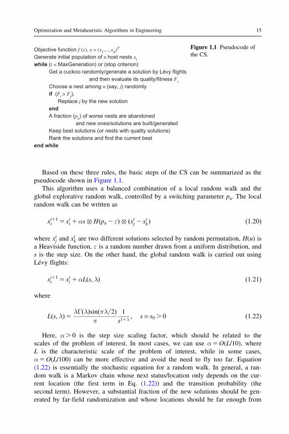
Based on these three rules, the basic steps of the CS can be summarized as the

pseudocode shown in Figure 1.1.

This algorithm uses a balanced combination of a local random walk and the

global explorative random walk, controlled by a switching parameter pa. The local

random walk can be written as

xt11i 5 xti 1αs� Hðpa 2 εÞ � ðxtj 2 xtkÞ ð1:20Þ

where xtj and xtk are two different solutions selected by random permutation, H(u) is

a Heaviside function, ε is a random number drawn from a uniform distribution, and

s is the step size. On the other hand, the global random walk is carried out using

Levy flights:

xt11i 5 xti 1αLðs;λÞ ð1:21Þ

where

Lðs;λÞ5 λΓðλÞsinðπλ=2Þπ

1

s11λ ; scs0 . 0 ð1:22Þ

Here, α. 0 is the step size scaling factor, which should be related to the

scales of the problem of interest. In most cases, we can use α5O(L/10), where

L is the characteristic scale of the problem of interest, while in some cases,

α5O(L/100) can be more effective and avoid the need to fly too far. Equation

(1.22) is essentially the stochastic equation for a random walk. In general, a ran-

dom walk is a Markov chain whose next status/location only depends on the cur-

rent location (the first term in Eq. (1.22)) and the transition probability (the

second term). However, a substantial fraction of the new solutions should be gen-

erated by far-field randomization and whose locations should be far enough from

Objective function f (x), x = (x1,...,xd)T

Generate initial population of n host nests xi

while (t < MaxGeneration) or (stop criterion) Get a cuckoo randomly/generate a solution by Lévy flights and then evaluate its quality/fitness Fi

Choose a nest among n (say, j) randomly if (Fi > Fj), Replace j by the new solution end A fraction (pa) of worse nests are abandoned and new ones/solutions are built/generated Keep best solutions (or nests with quality solutions) Rank the solutions and find the current bestend while

Figure 1.1 Pseudocode of

the CS.


the current best solution to make sure that the system will not be trapped in a

local optimum (Yang and Deb, 2010).

The pseudocode given here is sequential; however, vectors should be used from

an implementation point of view, as vectors are more efficient than loops.

A Matlab implementation is given by Yang and can be downloaded.2 CS is very

efficient in solving engineering optimization problems (Gandomi et al., 2011).

1.3.11 Other Algorithms

There are many other metaheuristic algorithms that are equally popular and power-

ful, including Tabu search (Glover and Laguna, 1997), artificial immune system

(Farmer et al., 1986), and others (Koziel and Yang, 2011; Yang, 2010a,b).

The efficiency of metaheuristic algorithms can be attributed to the fact that they

imitate the best features in nature, especially the selection of the fittest in biological

systems that have evolved by natural selection over millions of years.

Two important characteristics of metaheuristics are intensification and diversifi-

cation (Blum and Roli, 2003). Intensification intends to search locally and more

intensively, while diversification makes sure the algorithm explores the search

space globally (and hopefully also efficiently). A fine balance between these two

components is very important to the overall efficiency and performance of an algo-

rithm. Too little exploration and too much exploitation could cause the system to

be trapped in local optima, which makes it very difficult or even impossible to find

the global optimum. On the other hand, if there is too much exploration but too lit-

tle exploitation, it may be difficult for the system to converge, which would slow

down the overall search performance. A proper balance itself is an optimization

problem, and one of the main tasks of designing new algorithms is to find an opti-

mal balance concerning this optimality and/or trade-off.

Furthermore, just exploitation and exploration are not enough. During the

search, we have to use a proper mechanism or criterion to select the best solutions.

The most common criterion is to use the Survival of the Fittest, i.e., to keep updat-

ing the solution with the best one found so far. In addition, a certain elitism is often

used, which ensures that the best or fittest solutions are not lost and are passed

onto the next generations.

1.4 Artificial Neural Networks

As we will see, artificial neural networks are in essence optimization algorithms,

working in different contexts (Yang, 2010a).

2 www.mathworks.com/matlabcentral/fileexchange/29809-cuckoo-search-cs-algorithm.


http://www.mathworks.com/matlabcentral/fileexchange/29809-cuckoo-search-cs-algorithm

1.4.1 Artificial Neurons

The basic mathematical model of an artificial neuron was first proposed by

W. McCulloch and W. Pitts in 1943, and this fundamental model is referred to as

the McCulloch�Pitts model. Other models and neural networks are based on it.

An artificial neuron with n inputs or impulses and an output yk will be activated if

the signal strength reaches a certain threshold θ. Each input has a corresponding

weight wi. The output of this neuron is given by

yl 5ΦXni51

wiui

!ð1:23Þ

where the weighted sum ξ5Pn

i51 wiui is the total signal strength, and Φ is the so-

called activation function, which can be taken as a step function. That is, we have

ΦðξÞ5 1 if ξ$ θ0 if ξ, θ

�ð1:24Þ

We can see that the output is only activated to a nonzero value if the overall sig-

nal strength is greater than the threshold θ.The step function has discontinuity; sometimes, it is easier to use a nonlinear,

smooth function called a Sigmoid function:

SðξÞ5 1

11 e2ξ ð1:25Þ

which approaches 1 as U!N and becomes 0 as U!2N. An interesting property

of this function is

S0ðξÞ5 SðξÞ½12 SðξÞ� ð1:26Þ

1.4.2 Neural Networks

A single neuron can perform only a simple task—it is either on or off. Complex

functions can be designed and performed using a network of interconnecting neu-

rons or perceptrons. The structure of a network can be complicated, and one of the

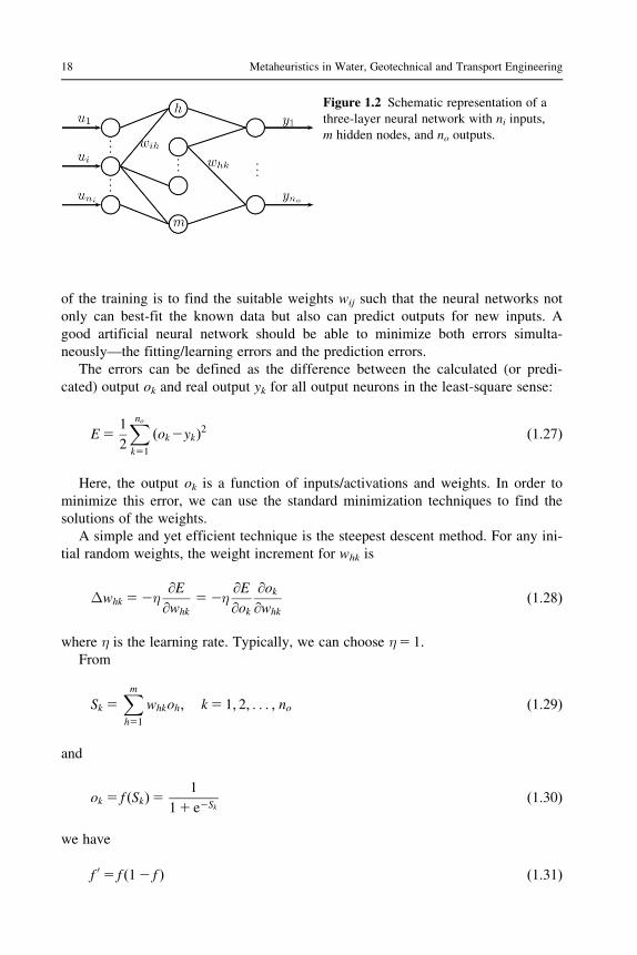
most widely used is to arrange them in a layered structure, with an input layer, an

output layer, and one or more hidden layers (Figure 1.2). The connection strength

between two neurons is represented by its corresponding weight. Some artificial

neural networks (ANNs) can perform complex tasks and can simulate complex

mathematical models, even if there is no explicit functional form mathematically.

Neural networks have been developed over the last few decades and applied in

almost all areas of science and engineering.

The construction of a neural network involves the estimation of the

suitable weights of a network system with some training/known data sets. The task


of the training is to find the suitable weights wij such that the neural networks not

only can best-fit the known data but also can predict outputs for new inputs. A

good artificial neural network should be able to minimize both errors simulta-

neously—the fitting/learning errors and the prediction errors.

The errors can be defined as the difference between the calculated (or predi-

cated) output ok and real output yk for all output neurons in the least-square sense:

E51

2

Xnok51

ðok2ykÞ2 ð1:27Þ

Here, the output ok is a function of inputs/activations and weights. In order to

minimize this error, we can use the standard minimization techniques to find the

solutions of the weights.

A simple and yet efficient technique is the steepest descent method. For any ini-

tial random weights, the weight increment for whk is

Δwhk 52η@E

@whk

52η@E

@ok

@ok@whk

ð1:28Þ

where η is the learning rate. Typically, we can choose η5 1.

From

Sk 5Xmh51

whkoh; k5 1; 2; . . . ; no ð1:29Þ

and

ok 5 f ðSkÞ51

11 e2Skð1:30Þ

we have

f 0 5 f ð12 f Þ ð1:31Þ

Figure 1.2 Schematic representation of a

three-layer neural network with ni inputs,

m hidden nodes, and no outputs.


@ok@whk

5@ok@Sk

@Sk@whk

5 okð12 okÞoh ð1:32Þ

and

@E

@ok5 ðok 2 ykÞ ð1:33Þ

Therefore, we have

Δwhk 52ηδkoh; δk 5 okð12 okÞðok 2 ykÞ ð1:34Þ

1.4.3 The Back Propagation Algorithm

There are many ways of calculating weights by supervised learning. One of the

simplest and widely used methods is to use the back propagation algorithm for

training neural networks, often called back propagation neural networks (BPNNs).

The basic idea is to start from the output layer and propagate backward to esti-

mate and update the weights. From any initial random weighting matrices wih

(for connecting the input nodes to the hidden layer) and whk (for connecting the hid-

den layer to the output nodes), we can calculate the outputs of the hidden layer oh:

oh 51

11 exp 2Pni

i51 wihui� � ; h5 1; 2; . . . ; m ð1:35Þ

and the outputs for the output nodes:

ok 51

11 exp 2Pm

h51 whkoh� � ; k5 1; 2; . . . ; no ð1:36Þ

The errors for the output nodes are given by

δk 5 okð12 okÞðyk 2 okÞ; k5 1; 2; . . . ; no ð1:37Þ

where yk(k5 1,2,. . ., no) are the data (real outputs) for the inputs ui(i5 1,2,. . ., ni).Similarly, the errors for the hidden nodes can be written as

δh 5 ohð12 ohÞXnok51

whkδk; h5 1; 2; . . . ; m ð1:38Þ

The updating formulas for weights at iteration t are

wt11hk 5wt

hk 1 ηδkoh ð1:39Þ


and

wt11ih 5wt

ih 1 ηδhui ð1:40Þ

where 0, η# 1 is the learning rate.

Here, we can see that the weight increments are

Δwih 5 ηδhui ð1:41Þ

with similar updating formulas for whk. An improved version is to use the so-called

weight momentum α to increase the learning efficiency:

Δwih 5 ηδhui 1αwihðτ2 1Þ ð1:42Þ

where τ is an extra parameter. There are many good software packages for ANNs,

and there are dozens of good books fully dedicated to implementation. ANNs have

been very useful in solving problems in civil engineering (Alavi and Gandomi,

2011a,b; Gandomi and Alavi, 2011).

1.5 Genetic Programming

Genetic programming is a systematic method of using evolutionary algorithms to

produce computer programs in a Darwinian manner. Fogel was probably one of the

pioneers in primitive genetic programming (Fogel et al., 1966), as he first used evo-

lutionary algorithms to study finite-state automata. However, the true formulation

of modern genetic programming was introduced and pioneered by Koza (1992),

and the publication of his book Genetic Programming: On the Programming of

Computers by Means of Natural Selection was a major milestone.

In essence, genetic programming intends to evolve computer programs in an

iterative manner by chromosome representations, often in terms of tree structures

where each node corresponds a mathematical operator and end nodes represent

operands. Evolution is carried out by genetic operators such as crossover, mutation,

and selection of the fittest. In the tree-structured representation, crossover often

takes the form of subtree exchange crossover, while mutation may take the form of

subtree replacement mutation.

According to Koza (1992), there are three stages in the process: preparatory

steps, a genetic programming engine, and a new computer program. The genetic

programming engine has preparatory steps as inputs and a computer program as

its output. First, we have to specify a set of primitive ingredients such as the func-

tion set and terminal set. For example, if we wish a computer program to be able

to design an electronic circuit, we have to specify the basic components such as

transistors, capacitors, and resistors, and their basic functions. Then we have to pro-

duce a fitness measure (such as time, cost, stability, and performance) to define


what solutions are better than others by that measure. In addition, we have to

produce some initialization of algorithm-dependent parameters, such as population

size and number of generations, and the termination criteria, which essentially

controls when the evolution should stop.

Though computationally expansive, genetic programming has aleady produced

human-competitive novel results in many areas such as electronic design, game

playing, quantum computing, and invention generation. New invention often

requires illogical steps in producing new ideas, and this can often be mimicked as a

randomization process in evolutionary algorithms. As pointed out by Koza et al.

(2003), genetic programming is a systematic method for getting computers to solve

a problem automatically, starting from a high-level statement outlining what needs

to be done, which virtually turns a computer into an “automated invention

machine.” Obviously, that is the ultimate aim of genetic programming.

For applications in engineering, readers can use more specialized literature

(Alavi and Gandomi, 2011a,b; Gandomi and Alavi, 2012a,b). There is an extensive

literature concerning genetic programming; interested readers can refer to works

such as Koza (1992) and Langdon (1998).

References

Afshar, A., Haddad, O.B., Marino, M.A., Adams, B.J., 2007. Honey-bee mating optimiza-

tion (HBMO) algorithm for optimal reservoir operation. J. Franklin Inst. 344,

452�462.

Alavi, A.H., Gandomi, A.H., 2011a. Prediction of principal ground-motion parameters using

a hybrid method coupling artificial neural networks and simualted annealing. Comput.

Struct. 89 (23�24), 2176�2194.

Alavi, A.H., Gandomi, A.H., 2011b. A robust data mining approach for formulation of

geotechnical engineering systems. Eng. Comput. 28 (3), 242�274.

Apostolopoulos, T., Vlachos, A., 2011. Application of the firefly algorithm for solving the eco-

nomic emissions load dispatch problem. Int. J. Combinatorics. 2011, Article ID 523806.

,http://www.hindawi.com/journals/ijct/2011/523806.html.. Accessed: 15 March 2012.

Blum, C., Roli, A., 2003. Metaheuristics in combinatorial optimization: overview and

conceptual comparison. ACM Comput. Surv. 35, 268�308.

Conn, A.R., Schneinberg, K., Vicente, L.N., 2009. Introduction to Derivative-Free

Optimization, MPS-SIAM Series on Optimization. SIAM, Philadelphia, PA.

Dorigo, M., Stutle, T., 2004. Ant Colony Optimization. MIT Press, Cambridge, MA, USA.

Farmer, J.D., Packard, N., Perelson, A., 1986. The immune system, adapation and machine

learning. Physica D. 2, 187�204.

Fogel, L.J., Owens, A.J., Walsh, M.J., 1966. Artificial Intelligence Through Simulated

Evolution. John Wiley & Sons, New York, NY.

Gandomi, A.H., Alavi, A.H., 2011. Applications of computation intelligence in behaviour

simulation of concrete maerials. In: Yang, X.S., Koziel, S. (Eds.), Computational

Optimization and Applications in Engineering and Industry. Studies in Computational

Intelligence, vol. 359. Springer, Heidelberg, Germany, pp. 221�243.


http://www.hindawi.com/journals/ijct/2011/523806.html

Gandomi, A.H., Alavi, A.H., 2012a. A new multi-gene genetic programming approach to

nonlinear system modeling. Part I: Materials and structural engineering. Neural

Comput. Appl. 21 (1), 171�187.

Gandomi, A.H., Alavi, A.H., 2012b. A new multi-gene genetic programming approach to

nonlinear system modeling. Part II: Geotechnical and earthquake engineering. Neural

Comput. Appl. 21 (1), 189�201.

Gandomi, A.H., Yang, X.S., Alavi, A.H., 2011. Mixed variable structural optimization using

firefly algorithm. Comput. Struct. 89 (23�24), 2325�2336.

Gandomi, A.H., Yang, X.S., Alavi, A.H., 2011. Cuckoo search algorithm: a metaheuristic

approach to solve structural optimization problems. Engineering With Computers. 27,

1�19. doi: 10.1007/s00366-011-0241-y.

Geem, Z.W., Kim, J.H., Loganathan, G.V., 2001. A new heuristic optimization: harmony

search. Simulation. 76, 60�68.

Glover, F., Laguna, M., 1997. Tabu Search. Kluwer Academic Publishers, Boston, MA.

Goldberg, D.E., 1989. Genetic Algorithms in Search, Optimization and Machine Learning.

Addison Wesley, Reading, MA.

Holland, J., 1975. Adaptation in Natural and Artificial Systems. University of Michigan

Press, Ann Arbor, MI.

Karaboga, D., 2005. An idea based on honey bee swarm for numerical optimization.

Technical Report TR06. Erciyes University, Turkey.

Karmarkar, N., 1984. A new polynomial-time algorithm for linear programming.

Combinatorica. 4 (4), 373�395.

Kennedy, J., Eberhart, R.C., 1995. Particle swarm optimization. In: Proceedings of IEEE

International Conference on Neural Networks. Piscataway, NJ, pp. 1942�1948.

Kennedy, J., Eberhart, R.C., Shi, Y., 2001. Swarm Intelligence. Morgan Kaufmann

Publishers, San Francisco.

Kirkpatrick, S., Gelatt, C.D., Vecchi, M.P., 1983. Optimization by simulated annealing.

Science. 220 (4598), 671�680.

Koza, J.R., 1992. Genetic Programming: On the Programming of Computers by Means of

Natural Selection. MIT Press, Cambridge, MA, USA.

Koza, J.R., Keane, M.A., Streeter, M.J., Yu, J., Lanza, G., 2003. Genetic Computing IV:

Routine Human-Competitive Machine Intelligence. Kluwer Academic Publishers,

Norwell, MA, USA.

Koziel, S., Yang, X.S., 2011. Computational Optimization, Methods and Algorithms.

Springer, Germany.

Langdon, W.B., 1998. Genetic Programming1Data Structures5Automatic Programming!.

Kluwer Academic Publishers, Norwell, MA, USA.

Nakrani, S., Tovey, C., 2004. On honey bees and dynamic server allocation in internet host-

ing centers. Adapt. Behav. 12 (3�4), 223�240.

Nelder, J.A., Mead, R., 1965. A simplex method for function optimization. Comput. J. 7,

308�313.

Parpinelli, R.S., Lopes, H.S., 2011. New inspirations in swarm intelligence: a survey. Int.

J. Bio-Inspired Comput. 3, 1�16.

Pavlyukevich, I., 2007. Levy flights, non-local search and simulated annealing. J. Comput.

Phys. 226, 1830�1844.

Pham, D.T., Ghanbarzadeh, A., Koc, E., Otri, S., Rahim, S., Zaidi, M., 2006. The bees

algorithm: a novel tool for complex optimisation problems. In: Proceedings of IPROMS

2006 Conference, pp. 454�461.


Price, K., Storn, R., Lampinen, J., 2005. Differential Evolution: A Practical Approach to

Global Optimization. Springer, Heidelberg, Germany.

Sawaragi, Y., Nakayama, H., Tanino, T., 1985. Theory of Multiobjective Optimisation.

Academic Press, Orlando, FL, USA.

Sayadi, M.K., Ramezanian, R., Ghaffari-Nasab, N., 2010. A discrete firefly meta-heuristic

with local search for makespan minimization in permutation flow shop scheduling

problems. Int. J. Ind. Eng. Comput. 1, 1�10.

Storn, R., 1996. On the usage of differential evolution for function optimization. In: Biennial

Conference of the North American Fuzzy Information Processing Society (NAFIPS),

pp. 519�523.

Storn, R., Price, K., 1997. Differential evolution—a simple and efficient heuristic for global

optimization over continuous spaces. J. Global Optim. 11, 341�359.

Talbi, E.G., 2009. Metaheuristics: From Design to Implementation. John Wiley & Sons,

Hoboken, NJ, USA.

Wolpert, D.H., Macready, W.G., 1997. No free lunch theorems for optimization. IEEE

Trans. Evol. Comput. 1, 67�82.

Yang, X.S., 2005. Engineering optimization via nature-inspired virtual bee algorithms. In:

Mira, J. and Alvarez, J.R. (Eds.), Artificial Intelligence and Knowledge Engineering

Applications: A Bioinspired Approach. Lecture Notes in Computer Science, vol. 3562.

Springer, Berlin/Heidelberg, pp. 317�323.

Yang, X.S., 2008. Nature-Inspired Metaheuristic Algorithms. first ed. Luniver Press, Frome.

Yang, X.S., 2009. Firefly algorithms for multimodal optimization. In: Watanabe,

O., Zeugmann, T. (Eds.), 5th Symposium on Stochastic Algorithms, Foundation and

Applications (SAGA 2009). LNCS, vol. 5792, Sapporo, Japan, pp. 169�178.

Yang, X.S., 2010a. Nature-Inspired Metaheuristic Algoirthms. second ed. Luniver Press,

Frome.

Yang, X.S., 2010b. Engineering Optimization: An Introduction with Metaheuristic

Applications. John Wiley & Sons, Hoboken, NJ, USA.

Yang, X.S., 2010c. A new metaheuristic bat-inspired algorithm, In: Gonzalez, J.R., Pelta, D.A.,

Cruz, C., Terrazas G., Krasnogor N. (Eds.), Nature-Inspired Cooperative Strategies for

Optimization (NICSO 2010). Studies in Computational Intelligence, vol. 284. Springer,

pp. 65�74.

Yang, X.S., 2011a. Bat algorithm for multi-objective optimisation. Int. J. Bio-Inspired

Comput. 3 (5), 267�274.

Yang, X.S., 2011b. Chaos-enhanced firefly algorithm with automatic parameter tuning. Int.

J. Swarm Intell. Res. 2 (4), 1�11.

Yang, X.S., Deb, S., 2009. Cuckoo search via Levy flights. In: Proceedings of World

Congress on Nature and Biologically Inspired Computing (NaBic 2009). IEEE

Publications, USA, pp. 210�214.

Yang, X.S., Deb, S., 2010. Engineering optimization by cuckoo search. Int. J. Math. Model.

Numer. Optim. 1 (4), 330�343.

Yang, X.S., Gandomi, A.H., 2012. Bat algorithm: a novel approach for global engineering

optimization. Eng. Comput. 29 (5), 1�18.

Yang, X.S., Koziel, S., 2011. Computational Optimization and Applications in Engineering

and Industry. Springer, Germany.


metaheuristics in water, geotechnical and transport engineering || optimization and metaheuristic...

Documents