Metaheuristic – Metaheuristic – Threshold Acceptance (TA)Threshold Acceptance (TA)

2

OutlinesOutlines

▪ Measuring Computational Efficiency▪ Construction Heuristics▪ Local Search Algorithms▪ Metaheuristic –

Threshold Accepting Algorithm (TA)▪ Traveling Salesman Problem (TSP)

3

Measuring Computational EfficiencyMeasuring Computational Efficiency

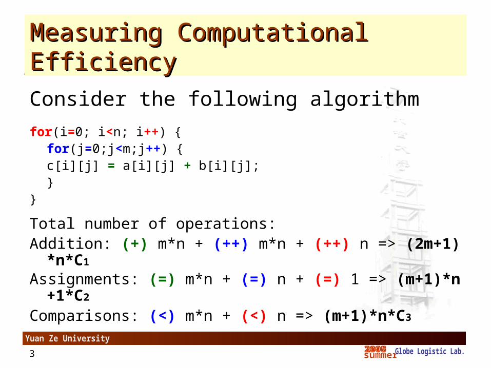
Consider the following algorithm

for(i=0; i<n; i++) {for(j=0;j<m;j++) {

c[i][j] = a[i][j] + b[i][j];}

}

Total number of operations: Addition: (+) m*n + (++) m*n + (++) n => (2m+1)*n*C1

Assignments: (=) m*n + (=) n + (=) 1 => (m+1)*n +1*C2

Comparisons: (<) m*n + (<) n => (m+1)*n*C3

4

Measuring Computational EfficiencyMeasuring Computational Efficiency

Which one is faster?

(a) (b)

5

Measuring Computational EfficiencyMeasuring Computational Efficiency

▪ Running Timelog(n) < n < n2 < n3 < 2n < 3n

6

Measuring Computational EfficiencyMeasuring Computational Efficiency

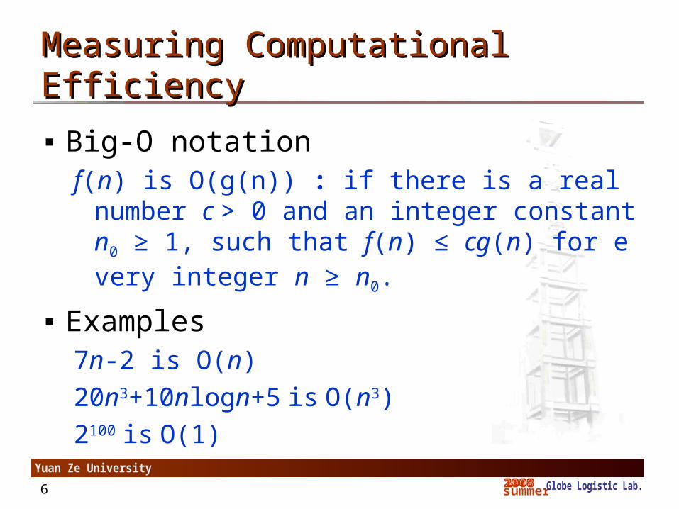
▪ Big-O notationf(n) is O(g(n)) : if there is a real number c > 0 and an

integer constant n0 ≥ 1, such that f(n) ≤ cg(n) for every integer n ≥ n0.

▪ Examples7n-2 is O(n)

20n3+10nlogn+5 is O(n3)

2100 is O(1)

7

Measuring Computational EfficiencyMeasuring Computational Efficiency

▪Big-O notation

O(log(n)) < O(n) < O(n log(n)) <O(n2) < O(n3) <O(2n) <O(3n)

logarithmic linear polynomial exponential

O(log n) O(n) O(nk), k ≥1 O(an), a ≥1

8

Traveling Salesman Problem (TSP)Traveling Salesman Problem (TSP)

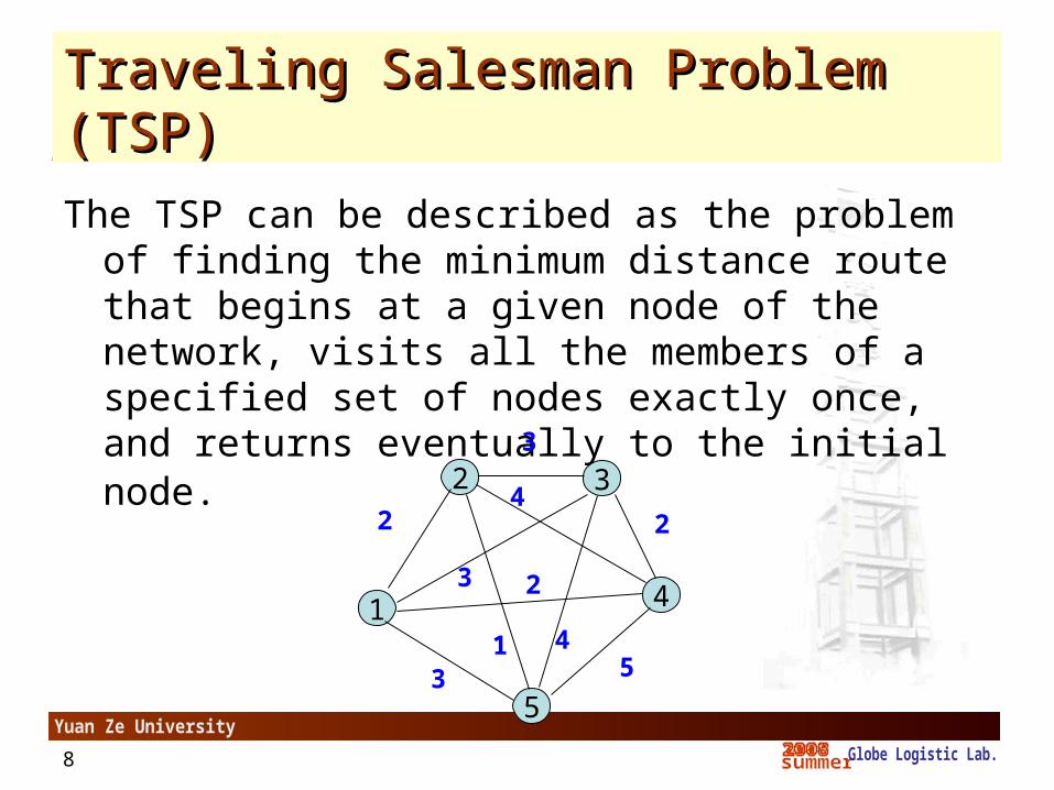
The TSP can be described as the problem of finding the minimum distance route that begins at a given node of the network, visits all the members of a specified set of nodes exactly once, and returns eventually to the initial node.

2 3

1 4

53 5

2

3

2

1

3 2

4

4

9

Construction HeuristicsConstruction Heuristics

▪ Greedy Algorithms:▪ Using an index to fix the priority for solving the

problem▪ Less flexibility to reach optimal solution▪ Constructing an initial solution for improvement

algorithms

▪ Example:▪ Northwest corner and minimum cost matrix for

transportation problem

10

Construction HeuristicsConstruction Heuristics

▪ Nearest neighbor procedure – O(n2)▪ Nearest insertion – O(n2)▪ Furthest insertion – O(n2)▪ Cheapest insertion – O(n3)

or – O(n2logn) (using heap)

11

Construction HeuristicsConstruction Heuristics

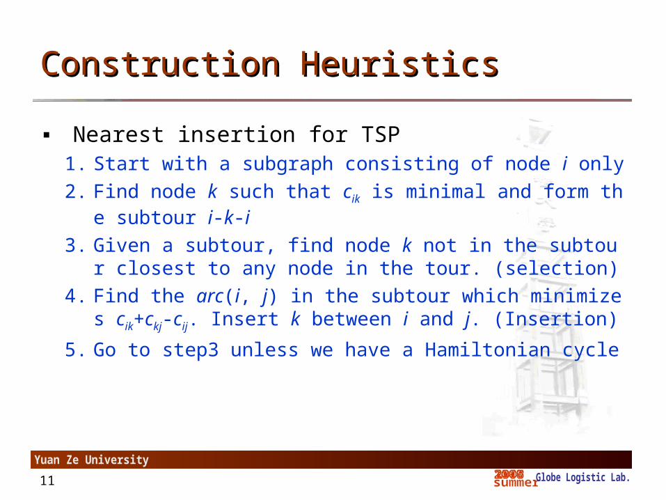
▪ Nearest insertion for TSP1. Start with a subgraph consisting of node i only

2. Find node k such that cik is minimal and form the subtour i-k-i

3. Given a subtour, find node k not in the subtour closest to any node in the tour. (selection)

4. Find the arc(i, j) in the subtour which minimizes cik+ckj-cij. Insert k between i and j. (Insertion)

5. Go to step3 unless we have a Hamiltonian cycle

12

Construction HeuristicsConstruction Heuristics

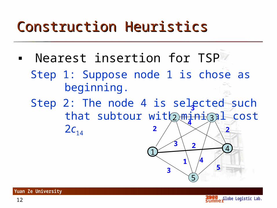
▪ Nearest insertion for TSPStep 1: Suppose node 1 is chose as beginning.

Step 2: The node 4 is selected such that subtour with minimal cost 2c14

2 3

1 4

53 5

2

3

2

1

3 2

4

4

13

Construction HeuristicsConstruction Heuristics

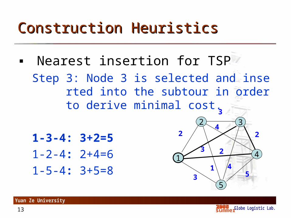
▪ Nearest insertion for TSPStep 3: Node 3 is selected and inserted into the subto

ur in order to derive minimal cost.

1-3-4: 3+2=5

1-2-4: 2+4=6

1-5-4: 3+5=8

2 3

1 4

53 5

2

3

2

1

3 2

4

4

14

Construction HeuristicsConstruction Heuristics

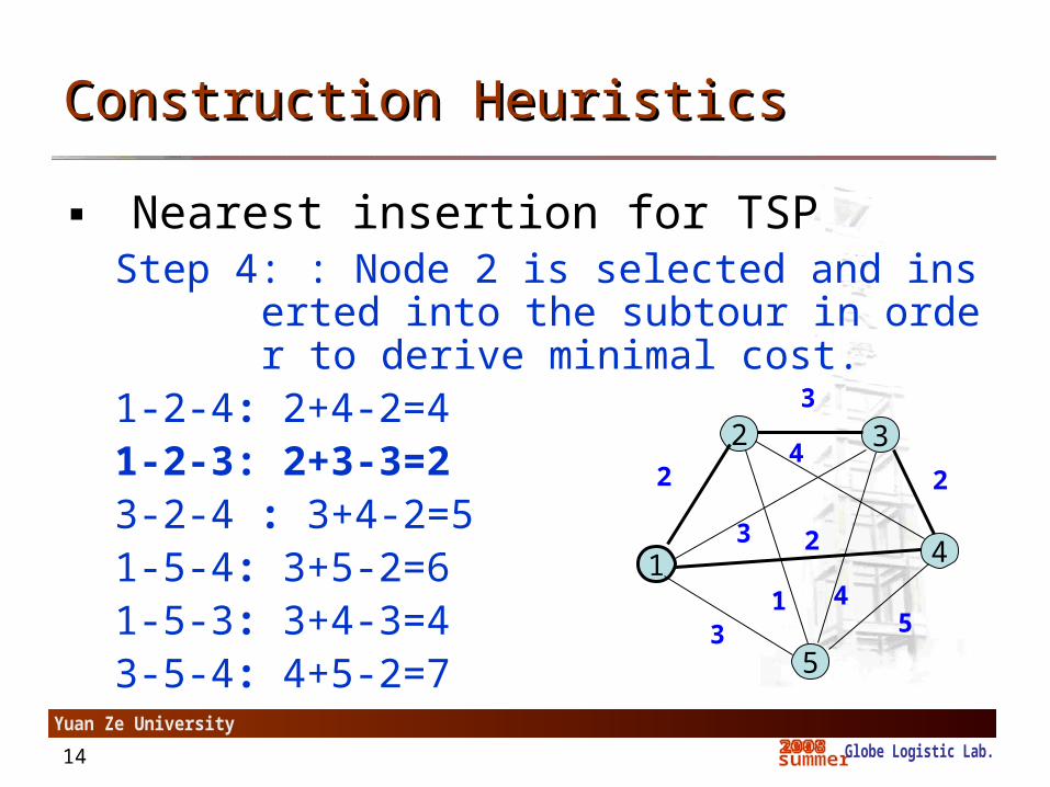
▪ Nearest insertion for TSPStep 4: : Node 2 is selected and inserted into the subt

our in order to derive minimal cost. 1-2-4: 2+4-2=41-2-3: 2+3-3=23-2-4 : 3+4-2=51-5-4: 3+5-2=61-5-3: 3+4-3=43-5-4: 4+5-2=7

2 3

1 4

53 5

2

3

2

1

3 2

4

4

15

Construction HeuristicsConstruction Heuristics

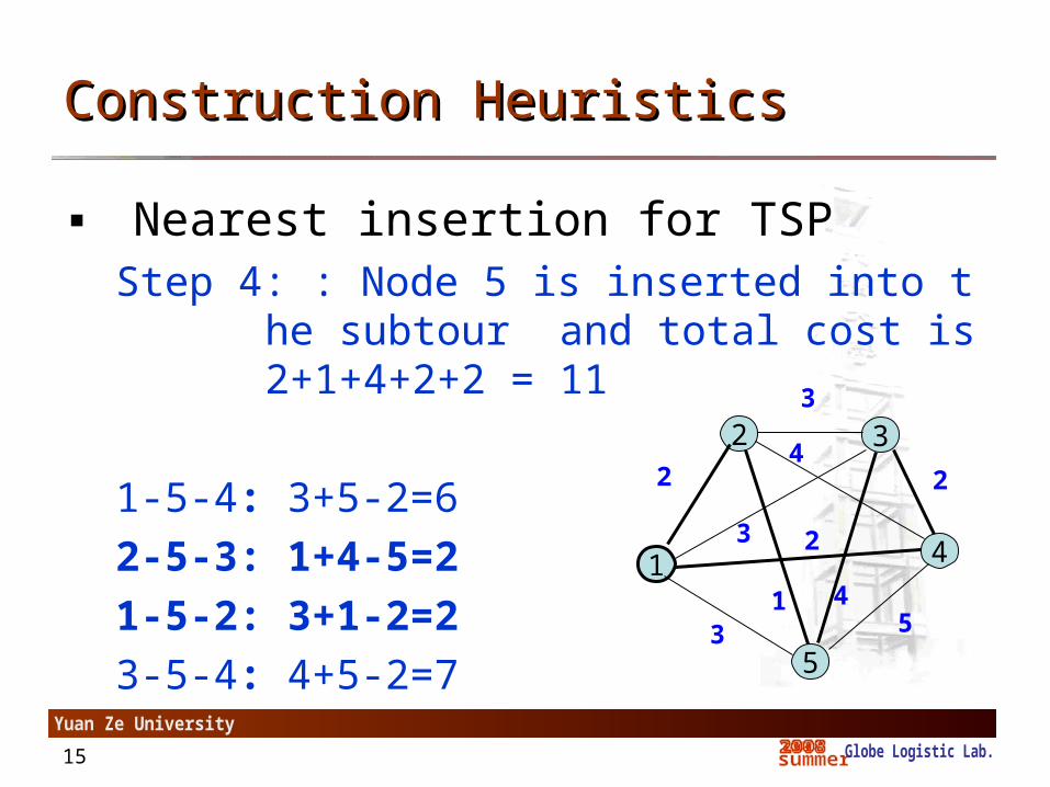
▪ Nearest insertion for TSPStep 4: : Node 5 is inserted into the subtour and total

cost is 2+1+4+2+2 = 11

1-5-4: 3+5-2=6

2-5-3: 1+4-5=2

1-5-2: 3+1-2=2

3-5-4: 4+5-2=7

2 3

1 4

53 5

2

3

2

1

3 2

4

4

16

Local Search AlgorithmsLocal Search Algorithms

▪ Simplex method▪ Convex

▪ Concave

17

Local Search AlgorithmsLocal Search Algorithms

▪ Integer linear programming▪ Combinatorial optimization:

▪ Knapsack Problem▪ TSP ▪ Vehicle routing problem

(VRP)

18

Local Search AlgorithmsLocal Search Algorithms

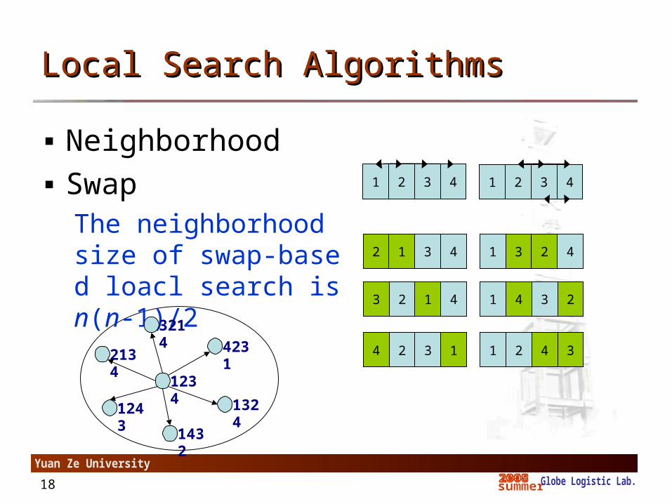
▪ Neighborhood▪ Swap

The neighborhood size of swap-based loacl search is n(n-1)/2

1 2 3 4

2 1 3 4

3 2 1 4

4 2 3 1

1324

4231

1234

1 2 3 4

1 3 2 4

1 4 3 2

1 2 4 3

3214

2134

1243

1432

19

Local Search AlgorithmsLocal Search Algorithms

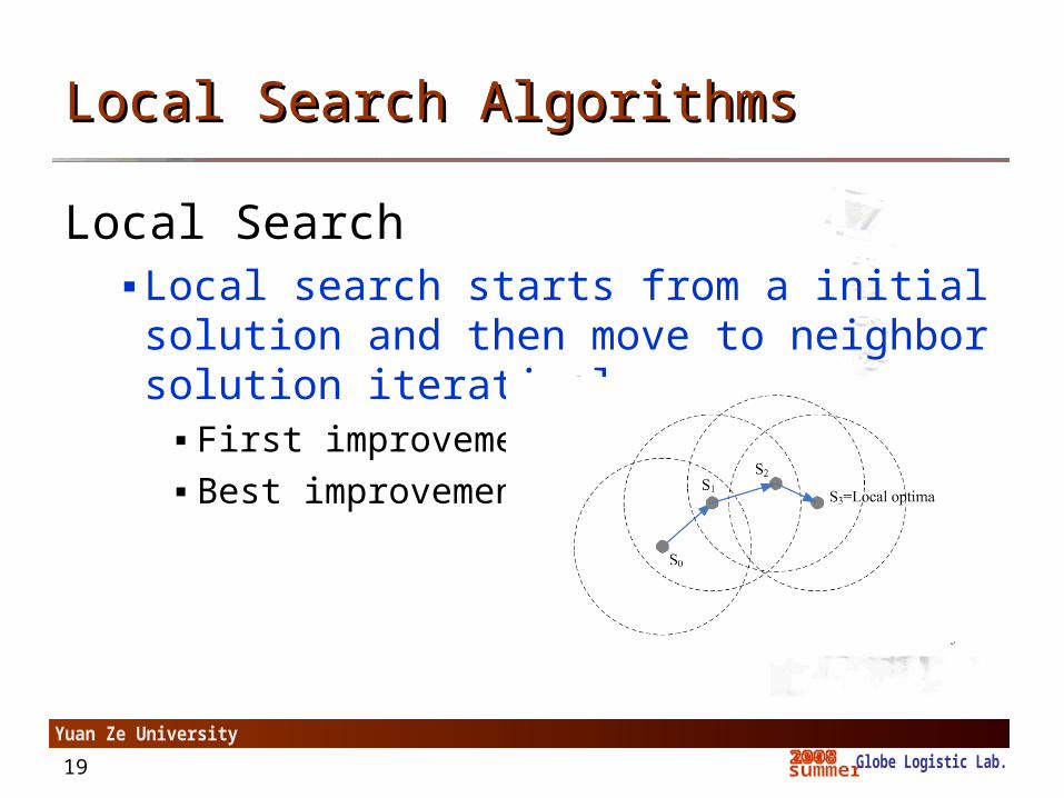
Local Search ▪ Local search starts from a initial solution and then

move to neighbor solution iteratively.▪ First improvement.▪ Best improvement.

20

Local Search AlgorithmsLocal Search Algorithms

Local Search for TSP▪ 2-opt▪ k-opt▪ OR-opt

21

Local Search AlgorithmsLocal Search Algorithms

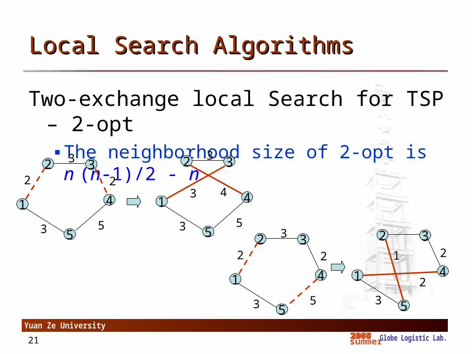
Two-exchange local Search for TSP – 2-opt▪ The neighborhood size of 2-opt is n (n-1)/2 - n

32 3

1 4

53 5

2 2

32 3

1 4

53 5

43

32 3

1 4

53 5

2 2

2 3

1 4

53

21

2

22

Local Search AlgorithmsLocal Search Algorithms

Implementation of 2-opt with array

1 2 3 4 5 6 7

1

2

54

3

6

71

2

54

3

6

7

1 2 5 4 3 6 7

23

Threshold Accepting Algorithm (TA) Threshold Accepting Algorithm (TA)

▪ Metaheuristic(巨集啟發式演算法 )▪ Threshold Accepting was proposed by De

uck and Scheuer (1990).Ref: G. Dueck, T. Scheuer, “Threshold accepting. A gene

ralpurpose optimization algorithm appearing superior tosimulated annealing”, Journal of Computational Physics 90 (1990) 161–175.

24

Threshold Accepting Algorithm (TA) Threshold Accepting Algorithm (TA)

▪ Metaheuristic(巨集啟發式演算法 )

solutions

objective

Local optimaglobe otima

25

Threshold Accepting Algorithm (TA) Threshold Accepting Algorithm (TA)

TA refined local search algorithms overcome the problem of getting tuck in a local optimal solution by admitting a temporary worsening of the objective function during the iteration process.

Initial solution

Generating a neighbor by a perturbation

∆f ≤ TH

reach number of iteration

no

reducing TH

yes

stop criteria satisfied

no

no

yse

stop

update best solution

yes

∆E0

1

probility

Threshold

Accepting probability