PHYSICAL REVIEW E 83, 021911 (2011)

Mechanical model of the ultrafast underwater trap of Utricularia

Marc Joyeux,* Olivier Vincent, and Philippe Marmottant†

Laboratoire de Spectrometrie Physique (CNRS UMR5588), Universite Joseph Fourier Grenoble 1, BP 87,F-38402 St Martin d’Heres, France

(Received 19 October 2010; published 18 February 2011)

The underwater traps of the carnivorous plants of the Utricularia species catch their prey through the repetitionof an “active slow deflation followed by passive fast suction” sequence. In this paper, we propose a mechanicalmodel that describes both phases and strongly supports the hypothesis that the trap door acts as a flexible valvethat buckles under the combined effects of pressure forces and the mechanical stimulation of trigger hairs, andnot as a panel articulated on hinges. This model combines two different approaches, namely (i) the description ofthin membranes as triangle meshes with strain and curvature energy, and (ii) the molecular dynamics approach,which consists of computing the time evolution of the position of each vertex of the mesh according to Langevinequations. The only free parameter in the expression of the elastic energy is the Young’s modulus E of themembranes. The values for this parameter are unequivocally obtained by requiring that the trap model fires, likereal traps, when the pressure difference between the outside and the inside of the trap reaches about 15 kPa.Among other results, our simulations show that, for a pressure difference slightly larger than the critical one, thedoor buckles, slides on the threshold, and finally swings wide open, in excellent agreement with the sequenceobserved in high-speed videos.

DOI: 10.1103/PhysRevE.83.021911 PACS number(s): 87.19.R−, 87.10.Tf, 62.20.mq

I. INTRODUCTION

There exist more than 600 species of carnivorous plants,which are the result of adaptation to poor environments interms of nutriments and/or sunshine [1]. The various methodsused by these plants to catch animals may be divided into twomain categories, namely active and passive traps, dependingon whether the capture of a prey does or does not involveany motion of the plant itself. Plants of the genus Nepenthesare typical examples of carnivorous plants with passive traps.Their catching mechanism relies mostly on the shape of thepitcherlike sleeves and the high viscoelasticity of the digestivefluid [2]. In contrast, the closure of the Venus flytrap leaf inabout 100 ms following mechanical stimulation of trigger hairsis a well-known example of an active trap [3].

Of the various active traps, none has, however, intriguedbotanists more than those of the about 215 species ofUtricularia [4–14]. These traps are aquatic, millimeter-sized,lenticular bladderlike organs [15,16] [see Fig. 1(a)]. They havean entrance, which remains closed by a door most of the time[see Figs. 1(b) and 1(c). Firing of the Utricularia trap is atwo-step mechanism. During the first, slow step, the dooris indeed closed and particular glands actively pump waterout of the trap interior. This has two consequences. First, thehydrostatic pressure inside the trap drops below that outsidethe trap by about 10–20 kPa [11,13]. Moreover, the concavewall curvature due to the lower internal pressure results inelastic energy being stored in the walls. We will show in thenext section that this deflation step is an essentially exponentialprocess with a time constant of about 1 h. The second, ultrafaststep starts when a potential prey touches one of the trigger hairsattached close to the center of the door. Then the door opens,and water (and the prey) is engulfed while the walls of the

*Marc.Joyeux@ujf-grenoble. fr†Philippe.Marmottant@ujf-grenoble. fr

trap release the stored energy and relax to their equilibriumposition. When the pressures inside and outside the trap areleveled, the door closes again autonomously.

We recently used a combination of high-speed videoimaging, scanning electron microscopy, light-sheet fluores-cence microscopy, particle tracking, and molecular dynamicssimulations, to visualize the motion of the door and proposea plausible mechanism. In particular, we observed that thetime span of suction is smaller than 1 ms, that is, substantiallyshorter than previously estimated [4]. We also measured amaximum liquid velocity of about 1.5 m s−1 and a maximumacceleration of 600 g, which leaves little escape chances tosmall prey. More importantly, our high-speed video recordings(up to about 10 000 frames per second), in combination withlight-sheet microscopy, reveal that the opening of the door ispreceded by the inversion of its curvature, and not the oppositeas was previously assumed [8]. After excitation of the triggerhairs, the (initially convex) door indeed bulges inside andbecomes concave, starting at the area of trigger hair insertion.It is only when this inversion of curvature has spread over thewhole door surface that the door opens and swings inside veryrapidly. These videos, which are available as supplementalmaterial of a separate article [17], therefore suggest that theextremely fast opening of the door is similar to the buckling ofa flexible valve [18] rather than the rotation of an almost rigidpanel articulated on hinges.

Most parts of these experimental results are published in abiology journal [17]. The purpose of the present complemen-tary paper is to show that the hypothesis of door bucklingis confirmed by molecular dynamics simulations based onthe description of the body and the door of the trap as thinmembranes with Young’s moduli in the range 2–10 MPa. Wewill provide a complete description of the model and the resultsobtained therewith.

We actually first show in Sec. II that important informationcan be extracted from experimental results by using a verysimple model, which consists of two parallel disks connected

021911-11539-3755/2011/83(2)/021911(12) ©2011 American Physical Society

MARC JOYEUX, OLIVIER VINCENT, AND PHILIPPE MARMOTTANT PHYSICAL REVIEW E 83, 021911 (2011)

by a spring. The remainder of the paper is then devoted to thedescription of the membrane model and the discussion of theresults obtained therewith. For the sake of faster calculations,we separated simulations concerning the body of the trap fromthose concerning the door and developed two different models,which, however, share many ingredients. The ingredientsthat are common to both models, that is, the expressions ofthe potential energy of the membrane and the equations ofevolution, are presented in Sec. III. The model for the trap bodyis then discussed in Sec. IV and that for the door in Sec. V.

II. A FIRST APPROACH: DISKS-AND-SPRING MODEL

In this section, we show that a very simple, scalar modelenables us to extract important information from experimentaldata.

A. Setting of the trap (deflation phase)

The model consists of describing the body of a trap astwo parallel disks of diameter L separated by a distance eand connected by a spring of constant k. It is assumed thatthe geometry of the trap remains that of a cylinder, that is,an impermeable and highly extensible membrane closes thevolume between the two disks. e represents the thickness ofthe trap. Experimentally, the traps are viewed from above (thatis, along the x axis of Fig. 1) and their thickness e is measuredclose to the center of the body, as is shown in the inset inthe top plot of Fig. 2. A typical curve for the time evolutionof e during setting (deflation) of an Utricularia inflata trap isshown in Fig. 2 on linear (top plot) and logarithmic (bottomplot) scales. The trap is fired manually and measurement ofe starts immediately after the ultrafast opening and closingof the door. The thickness of the trap is therefore maximum

(a) (b)

(c)

x

yz

x

y

door

body

x

y500 µm 500 µm

FIG. 1. (a) Stereo microscopy view of an Utricularia inflata trap.The door and the trigger hairs face the right edge of the picture.The other two pictures show lateral views of the door in closed(b) and open (c) positions, which were obtained with an ultrafastcamera. The black shadow at the upper right edge of the pictures isthe lever, which is used to manually excite trigger hairs and fire the trapmechanism.

e

0.4

0.5

0.6

0.7

0.8

0 100 200 30010-3

10-2

10-1

100

2346

2346

2346

time (minutes)

e -

e min

(m

m)

e (

mm

)

deflation phase

τ = 53 minutes

FIG. 2. (Color online) Deflation of the trap body. The plots showthe evolution of the thickness e of the trap (expressed in mm) asa function of time (expressed in minutes) on linear (top plot) andlogarithmic (bottom plot) scales. The trap is fired manually at timet = 0 and measurement of e starts immediately after the ultrafastclosing of the door. The insert in the top plot shows a trap closeto maximum deflation viewed from above and indicates where thethickness e is measured. The door of the trap faces the right edgeof the figure. The dot-dashed line in the bottom plot shows the resultof the least square adjustment with τpump = 53 min.

at t = 0. Figure 2 indicates that e evolves exponentially withtime, according to

e(t) = emin + (emax − emin) exp

(− t

τpump

), (2.1)

where emax is the thickness of the trap at rest (completelyinflated), emin is its thickness when it is completely deflatedand ready to fire, and τpump is the characteristic time forpumping. For the trap and the deflation event shown inFig. 2, we measured emax ≈ 0.80 mm, emin ≈ 0.37 mm, andτpump ≈ 53 min. Successive experiments performed with thissame trap led to values of τpump that varied by less than theuncertainty of the fit, that is, a few minutes. In contrast,measurements performed with different traps led to ratherdifferent values of τpump, which ranged from 28 to 53 min.This large scattering in the values of τpump is certainly due,in part, to differences in the size of the investigated traps, butit may also result from different efficiencies of the respectivesets of pumping glands. We also note in passing that the largevalue of the characteristic time for pumping obliged us to waitseveral hours between two successive experiments performedon the same trap, in order for the trap to be always in the same(almost) steady state when fired.

021911-2

MECHANICAL MODEL OF THE ULTRAFAST UNDERWATER . . . PHYSICAL REVIEW E 83, 021911 (2011)

The maximum pumping rate Q0, that is, the pumping rateat t = 0, can furthermore be estimated from

Q0 = −(

dV

dt

)t=0

= π

4L2 emax − emin

τpump, (2.2)

where V is the volume comprised between the two disks. Whenplugging in Eq. (2.2) the value L = 1.5 mm, as well as thosederived above for emin, emax, and τpump, one obtains Q0 ≈0.86 mm3 h−1, which compares well with the value reportedin Ref. [13], that is, Q0 ≈ 1.26 mm3 h−1. An upper limit for thehydraulic permeability of the trap walls, κh, can furthermorebe estimated by assuming that the pumping rate is constantand equal to Q0, and that transfers of liquid between the insideand the outside of the trap arise uniquely from the porosity ofthe walls. Then

κh = ηQ0h

2S�pmax= 2ηQ0h

πL2�pmax, (2.3)

where η is the viscosity of the fluid (η ≈ 10−3 Pas), h is thethickness of the wall, S is the surface of each disk, and �pmax

is the steady-state pressure difference between the inside andthe outside of the trap. When plugging h ≈ 100 μm and�pmax ≈ 15 kPa [11,13] in Eq. (2.3), one gets κh ≈ 45 A

2.

At last, the constant k of the spring is such that pressure forces2S�p and the spring elastic force k(emax − emin) cancel atmaximum deflation, that is, when �p = �pmax and e = emin.One therefore has

k = 2S�p

emax − emin= πL2�p

2(emax − emin), (2.4)

which leads to k = 120 J m−2. The elastic energy stored inthe membrane during the deflation phase, k

2 (emax − emin)2, isconsequently close to 11 μJ.

B. Firing of the trap (inflation phase)

Let us now consider the inflation of the trap once it ismanually triggered and the door opens. A typical curve forthe time evolution of e during the suction phase (inflation) ofan Utricularia inflata trap is shown in Fig. 3 on linear (topplot) and logarithmic (bottom plot) scales. Figure 3 indicatesthat the time evolution of e is not monoexponential, but mostof the gap to maximum thickness (or volume) is neverthelessbridged with a time constant of the order of 1 ms. Moreover,the maximum speed of the walls of the trap can be estimatedby taking the numerical derivative of the curve in the top plotof Fig. 3. One obtains (de/dt)max ≈ 0.14 m s−1. The variationof e can be related to the average speed u of the fluid enteringthe trap by considering that the door is a disk of radius r =300 μm. Conservation of volume then implies that

dV

dt= πr2u, (2.5)

which can be rewritten in the form

u =(

L

2r

)2de

dt. (2.6)

The maximum value of u deduced from the plots in Fig. 3is therefore umax ≈ 0.9 m s−1. One thereby recovers in acomparatively simpler way the result obtained by tracking

0.3

0.4

0.5

0.6

0.7

0.8

-2 0 2 4 6 8 10

10-2

10-1

2

3456

2

3456

time (ms)

e max

- e

(m

m)

e (

mm

)

inflation phase

τ = 1.3 ms

FIG. 3. (Color online) Inflation of the trap body after triggering.The plots show the evolution of the thickness e of the trap (expressedin mm) as a function of time (expressed in ms) on linear (top plot)and logarithmic (bottom plot) scales. The origin of the time scale issomewhat arbitrary. The dot-dashed line in the bottom plot shows theevolution of an exponential process with time constant τ = 1.3 ms.

the motion of hollow glass beads of density 1.1 and diameter6–20 μm initially dispersed in the fluid. The motion ofthese tracers during the suction phase was recorded using ahigh-speed Phantom Miro 4 camera (up to 8100 frames persecond for images with 256×256 pixels) placed on the sideof the traps, that is, along the z axis. These more elaborateexperiments lead to a maximum speed of the fluid of about1.5 m s−1 [17]. They additionally indicate that the accelerationof the fluid reaches the impressive value of 600 g.

The maximum Reynolds number along the flow, Re, writes

Re = 2rumax

ν, (2.7)

where ν = 10−6 m2 s−1 is the kinematic viscosity of water.One obtains Re ≈ 540, which indicates that the flow enteringthe trap is strongly inertial but still remains laminar, since fullydeveloped turbulence arises only for Reynolds numbers largerthan 2000 [19].

At last, one may estimate the characteristic inertial time fortrap inflation, τi , by considering that it is equal to one-fourthof the oscillation period of a mass m (equal to the mass ofone disk) attached to a spring with the constant k determinedabove, that is,

τi = π

2

√m

k. (2.8)

021911-3

MARC JOYEUX, OLIVIER VINCENT, AND PHILIPPE MARMOTTANT PHYSICAL REVIEW E 83, 021911 (2011)

The inertia of an object is larger in a liquid than in air,because of the mass of the liquid that is displaced during themotion of the object. Therefore m can be estimated as the massof the liquid that is displaced by each disk during inflationand deflation, that is, m = 1

2ρS(emax − emin), where ρ is thedensity of water. One obtains m ≈ 0.4 mg, and consequentlyτi ≈ 0.2 ms. This estimate of τi is one order of magnitudesmaller than the time it actually takes for the trap to inflate (seeFig. 3). This indicates that friction plays a crucial dynamicalrole in slowing down the inflation motion from the 0.1-ms timescale to the 1-ms one. We will come back later to this point.

The very simple disks-and-spring model therefore enablesone to estimate some of the principal characteristics of thetrap, namely the maximum pumping rate (about 1 mm3 h−1),the characteristic pumping time (about 1 h), the hydraulicpermeability of the membrane (a few tens of A

2), and the

average elastic energy stored in the membrane (in the μJrange). Moreover, it leads to the correct value for the maximumvelocity of the fluid (about 1 m s−1), and suggests that theobserved time scale of the dynamics (a few ms) is imposedby the frictions with the surrounding liquid and not by theinertia of the trap body itself. However, this model provides noindication concerning the actual mechanisms that enable suchastounding catching performances. This is essentially due tothe fact that it describes the body of the trap but completelydisregards the door, which is certainly the most intriguingpart of this plant. We therefore developed a more elaboratemembrane model, in order to get a better understanding of thedynamics of the trap.

III. MEMBRANE MODEL

The remainder of this paper is devoted to the description ofthe three-dimensional membrane model and the discussion ofthe results obtained therewith. For the sake of faster calcula-tions, we separated simulations concerning the body of the trapfrom those concerning its door and developed two differentmodels, which, however, share many ingredients. We describein the present section the ingredients that are common to bothmodels, that is, the expressions of the potential energy and theequations of evolution, as well as the discretization procedure.We postpone the complete presentation of the model for thetrap body to Sec. IV, and that for the door to Sec. V.

Both the trap body and the door are modeled as thinmembranes of thickness h, which are made of an isotropic,homogeneous, and incompressible material with Young’smodulus E and Poisson ratio ν = 1

2 . Note, however, that theYoung’s moduli of the body and the trap are not necessarilyidentical, because they are made of cells with different thick-ness and different spatial organization. The elastic potentialenergy stored in the deformation of the membrane Epot canbe written as the sum of a strain contribution Estrain and acurvature contribution Ecurv, according to [20,21]

Epot = Estrain + Ecurv,

Estrain = Eh

2(1 − ν2)

∫S

{(1 − ν)Tr(ε2) + ν[Tr(ε)]2} dS,

Ecurv = Eh3

24(1 − ν2)

∫S

{[Tr(b)]2 − 2(1 − ν)Det(b)} dS,

(3.1)

where S is the area of the membrane, ε is the two-dimensionalCauchy-Green local strain tensor [22], and b is the differencebetween the local curvature tensors of the strained membraneand the reference geometry (see below). For numericalpurposes, all membranes are described as triangle meshes withM triangles (facets) and N ≈ M/2 vertices. Denoting by δSn

the area of facet n, the elementary area δAj associated tovertex j is

δAj = 1

3

∑n∈V1(j )

δSn, (3.2)

where n ∈ V1(j ) means that the sum runs over all the facetsn that contain vertex j. Each vertex j is also associated witha mass mj , which is derived from the reference geometryaccording to

mj = ρhδAj , (3.3)

where ρ is the density of the membrane. We used ρ =1 kg dm−3, because the cells that form the membrane are filledwith water and the trap itself is very close to the floating limit.Use of a different value for ρ would only modify the kineticenergy proportionally and would not change qualitatively theresults presented below. The mass mj of each vertex is thenkept constant during the simulations, while area elements δSn

and δAj may vary. Estrain is discretized in the form

Estrain = Eh

2(1 − ν2)

M∑n=1

{(1 − ν)Tr

(ε2

n

) + ν[Tr(εn)]2}δSn,

(3.4)

where the Cauchy-Green strain tensor [22] for facet n, εn,writes

εn = 12

[Fn · (

F0n

)−1 − I]. (3.5)

In this equation, I denotes the 2×2 identity matrix, whileFn and F0

n are the Gram matrices for facet n in the strainedgeometry and the reference one, that is,

Fn =(

(rn2 − rn1) · (rn2 − rn1) (rn2 − rn1) · (rn3 − rn1)

(rn2 − rn1) · (rn3 − rn1) (rn3 − rn1) · (rn3 − rn1)

)

(3.6)

where rn1, rn2, and rn3 describe the positions of the threevertices of the facet.

The contribution to energy arising from curvature, Ecurv,is more difficult to evaluate. The terms containing Tr(b) andDet(b) in Eq. (3.1) are known as the mean curvature energyand the Gaussian curvature energy, respectively. They can berewritten in the more explicit form

Ecurv = Emean + EGauss,

Emean = Eh3

24(1 − ν2)

∫S

(c1 + c2 − c0

1 − c02

)2dS,

EGauss = − Eh3

12(1 + ν)

∫S

[(c1 − c0

1

)(c2 − c0

2

)(3.7)

− sin2 θ(c0

1 − c02

)(c1 − c2)

]dS,

where the ck and c0k (k = 1,2) are the local principal curvatures

of the strained membrane and those of the reference geometry,

021911-4

MECHANICAL MODEL OF THE ULTRAFAST UNDERWATER . . . PHYSICAL REVIEW E 83, 021911 (2011)

respectively, and θ is the angle by which the local principaldirections of the membrane have rotated with respect to thoseof the reference geometry. The mean curvature energy is ratherstraightforwardly discretized according to

Emean = Eh3

6(1 − ν2)

N∑j=1

(κj − κ0

j

)2δAj . (3.8)

In this equation, κj and κ0j represent the mean curvature

κ = (c1 + c2)/2 at vertex j for the strained membrane andthe reference geometry, respectively. They are estimated from[23,24]

κj = 1

4δAj

∥∥∥∥∥∥∑

k∈N1(j )

(cot αjk + cot βjk)(rk − rj )

∥∥∥∥∥∥ , (3.9)

where k ∈ N1(j ) means that the sum runs over the vertices kthat are directly connected to vertex j. rj and rk denote thepositions of vertices j and k, and αjk and βjk are the angles ofthe corners opposite to bond (jk) in the two facets that share thisbond. The problem actually arises from the Gaussian curvatureenergy, because it is difficult to estimate θ correctly in thecourse of a simulation. We consequently used an approximateexpression for EGauss, namely

EGauss ≈ − Eh3

12(1 + ν)

∫S

(c1c2 − c0

1c02 − 1

2

(c0

1 + c02

)× (

c1 + c2 − c01 − c0

2

))dS. (3.10)

Note that it is sufficient that c01 − c0

2 be equal to zeroeverywhere on the membrane for the expressions for EGauss

in Eqs. (3.7) and (3.10) to be equivalent. This is the case, inparticular, if the membrane has no spontaneous curvature (c0

1 =c0

2 = 0 everywhere) or if the reference geometry is a sphereof radius R (c0

1 = c02 = 1/R everywhere). Equation (3.10)

is finally discretized according to

EGauss ≈ − Eh3

12(1 + ν)

N∑j=1

[Gj − G0

j − 2κ0j

(κj − κ0

j

)]δAj .

(3.11)

In Eq. (3.11), Gj and G0j represent the Gaussian curvature

G = c1c2 at vertex j for the strained membrane and thereference geometry, respectively, which we estimate from [25]

Gj = 1

δAj

⎛⎝2π −

∑n∈V1(j )

γnj

⎞⎠ , (3.12)

where γnj denotes the angle at vertex j in facet n.At that point, the important question that arises is what are

the reference geometries, that is, those for which the Grammatrices F0

n and spontaneous curvatures κ0j and G0

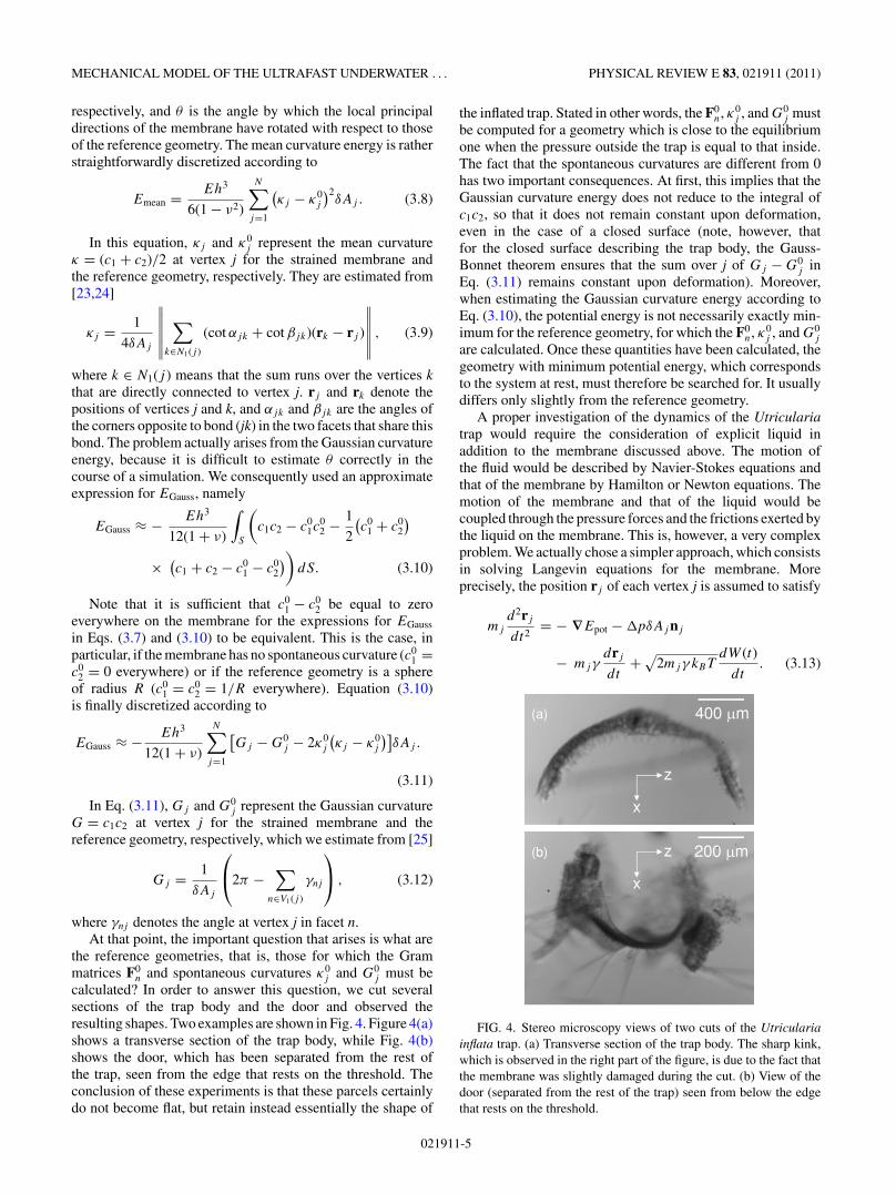
j must becalculated? In order to answer this question, we cut severalsections of the trap body and the door and observed theresulting shapes. Two examples are shown in Fig. 4. Figure 4(a)shows a transverse section of the trap body, while Fig. 4(b)shows the door, which has been separated from the rest ofthe trap, seen from the edge that rests on the threshold. Theconclusion of these experiments is that these parcels certainlydo not become flat, but retain instead essentially the shape of

the inflated trap. Stated in other words, the F0n, κ0

j , and G0j must

be computed for a geometry which is close to the equilibriumone when the pressure outside the trap is equal to that inside.The fact that the spontaneous curvatures are different from 0has two important consequences. At first, this implies that theGaussian curvature energy does not reduce to the integral ofc1c2, so that it does not remain constant upon deformation,even in the case of a closed surface (note, however, thatfor the closed surface describing the trap body, the Gauss-Bonnet theorem ensures that the sum over j of Gj − G0

j inEq. (3.11) remains constant upon deformation). Moreover,when estimating the Gaussian curvature energy according toEq. (3.10), the potential energy is not necessarily exactly min-imum for the reference geometry, for which the F0

n, κ0j , and G0

j

are calculated. Once these quantities have been calculated, thegeometry with minimum potential energy, which correspondsto the system at rest, must therefore be searched for. It usuallydiffers only slightly from the reference geometry.

A proper investigation of the dynamics of the Utriculariatrap would require the consideration of explicit liquid inaddition to the membrane discussed above. The motion ofthe fluid would be described by Navier-Stokes equations andthat of the membrane by Hamilton or Newton equations. Themotion of the membrane and that of the liquid would becoupled through the pressure forces and the frictions exerted bythe liquid on the membrane. This is, however, a very complexproblem. We actually chose a simpler approach, which consistsin solving Langevin equations for the membrane. Moreprecisely, the position rj of each vertex j is assumed to satisfy

mj

d2rj

dt2= − ∇Epot − �pδAj nj

− mjγdrj

dt+ √

2mjγ kBTdW (t)

dt. (3.13)

(a)

(b)

z

x

z

x

400 µm

200 µm

FIG. 4. Stereo microscopy views of two cuts of the Utriculariainflata trap. (a) Transverse section of the trap body. The sharp kink,which is observed in the right part of the figure, is due to the fact thatthe membrane was slightly damaged during the cut. (b) View of thedoor (separated from the rest of the trap) seen from below the edgethat rests on the threshold.

021911-5

MARC JOYEUX, OLIVIER VINCENT, AND PHILIPPE MARMOTTANT PHYSICAL REVIEW E 83, 021911 (2011)

In this equation, �p is the pressure outside the trap minusthe pressure inside, nj is the outward normal to the surface atvertex j, γ is the dissipation coefficient, and W (t) is a Wienerprocess. The first and second terms on the right-hand sideof Eq. (3.13) describe elastic and pressure forces, respectively,while the two last terms model the effects of the liquid, namelyfriction and thermal noise. Note that thermal noise (the lastterm) is negligibly small compared to elastic and pressureforces. nj is computed according to

nj =

∑n∈V1(j )

δSnun∥∥∥∥ ∑n∈V1(j )

δSnun

∥∥∥∥, (3.14)

where un is the outward normal to facet n. For numericalpurposes, the derivatives in Langevin equations are replacedby finite differences. The position of vertex j at time step i + 1,ri+1j , is consequently obtained from the positions r i

j and r i−1j

at the two previous time steps according to

mj

(1 + γ�t

2

)ri+1j = 2mj ri

j − mj

(1 − γ�t

2

)ri−1j

− (∇Epot + �pδAj nj )�t2

+√2mjγ kBT �t3/2w(t), (3.15)

where �t is the time step and w(t) is a normally distributedrandom function with zero mean and unit variance.

It is important to realize that the model described aboveactually depends on two adjustable parameters, namelythe Young’s modulus E, which determines the strengthof the elastic energy of the membrane in Eq. (3.1), and thedissipation coefficient γ , which determines the strength of theinteractions between the liquid and the membrane in Langevinequations (3.13). On the other side, experiments yield twofundamental quantities, namely the pressure difference �p

in set conditions (�p is in the range 10–20 kPa [11,13]),and the time scales at which the door opens (a few tenthsof ms) and the trap inflates (a few ms). As will be shownbelow, the Young’s moduli of the trap and door membranescan be unambiguously derived from the experimental valueof �p, while the value of γ is obtained by requiring that thedoor opening and trap inflation time scales computed withthe model match the observed ones. This is therefore a very

favorable case, where all the parameters of the model can bededuced from experiment.

IV. DYNAMICS OF THE TRAP BODY

As already mentioned, we separated, for the sake of fastercalculations, simulations performed for the trap body fromthose concerning the door. In this section, we describe themodel we developed for the trap body and the results obtainedtherewith. The model for the door will be discussed in thefollowing section.

A. Geometry of the trap

The trap body is modeled as a closed shell of thicknessh = 100 μm. It contains no aperture. The setting phase(deflation) is simulated by decreasing slowly the internalpressure relative to the external one. Once the trap is set,firing and the subsequent inflation are simulated by resettinginstantly to zero the pressure difference between the inside andthe outside of the trap.

The first question that arises is that of the geometry of thetrap body. By considering the shape of real traps, like the oneshown in Fig. 1(a), we first described the inflated trap as anoblate ellipsoid with major radius of 1 mm and minor radiusin the range 0.5–0.7 mm. However, results obtained with thisgeometry differ markedly from the observed behavior, for allrealistic values of the Young’s modulus E and the dissipationcoefficient γ . Such simulations indeed predict that deflationconsists of a single, abrupt buckling of the membrane, whileobservation instead leads to the conclusion that deflation is anessentially smooth and continuous process, although it seemsthat some limited buckling of small portions of the surfacesometimes occur. This difference is due to the fact that the realtrap is not convex everywhere but contains instead regions withnegative curvature even in the inflated geometry. These regionswith negative curvature actually act as seeds from whichdeflation propagates like a rolling wave when the internalpressure is decreased.Therefore we introduced such regionswith negative curvature in our model by considering that thegeometry of the inflated trap is obtained by transforming thecoordinates (xj ,yj ,zj ) of the vertices of a triangulated sphereof radius 1 mm according to

⎛⎜⎝

xj

yj

zj

⎞⎟⎠ →

⎛⎜⎝

xj

yj − 0.1(y2

j − z2j

)0.55zj − 0.12

(1 − x2

j

)[sin

(32

)zj + 2 sin(3)yj zj + sin

(92

)zj

(3y2

j − z2j

) + 4 sin(6)yj zj

(y2

j − z2j

)]⎞⎟⎠ . (4.1)

The transformation of Eq. (4.1) may look rather arbitrary,especially for the zj coordinate. However, the trigonometricterms that appear in this equation are just the first terms of theFourier expansion of a Dirac peak and are aimed at creatinga region with negative curvature on both sides of the trap.Moreover, the overall shape of the trap body is convincinglyreproduced with this expression. The F0

n, κ0j , and G0

j are

calculated for this geometry and the geometry corresponding tothe minimum of the potential energy is then searched for. Fromthe practical point of view, and unless otherwise stated, we useda mesh with about N ≈ 2150 vertices and M ≈ 4300 facets.For this mesh, the minimum energy geometry corresponds to apotential energy Epot ≈ −0.89 μJ and is only slightly differentfrom that described by Eq. (4.1). It is shown in the left picture

021911-6

MECHANICAL MODEL OF THE ULTRAFAST UNDERWATER . . . PHYSICAL REVIEW E 83, 021911 (2011)

Vred = 1.00 Vred = 0.60

xz

y

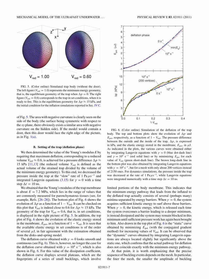
FIG. 5. (Color online) Simulated trap body (without the door).The left figure (Vred = 1.0) represents the minimum energy geometry,that is, the equilibrium geometry of the trap when �p = 0. The rightfigure (Vred = 0.6) corresponds to the trap in set conditions, when it isready to fire. This is the equilibrium geometry for �p ≈ 15 kPa, andthe initial condition for the inflation simulations reported in Sec. IV C.

of Fig. 5. The area with negative curvature is clearly seen on theside of the body (the surface being symmetric with respect tothe xy plane, there obviously exists a similar area with negativecurvature on the hidden side). If the model would contain adoor, then this door would face the right edge of the picture,as in Fig. 1(a).

B. Setting of the trap (deflation phase)

We then determined the value of the Young’s modulus E byrequiring that maximum deflation, corresponding to a reducedvolume Vred ≈ 0.6, is achieved for a pressure difference �p ≈15 kPa [11,13] (the reduced volume Vred is defined as theactual volume of the strained trap divided by the volume ofthe minimum energy geometry). To this end, we decreased thepressure inside the trap at the “slow” rate of 1 Pa μs−1 andintegrated Langevin equations (3.15) for γ = 0 with a timestep �t = 10 ns.

We obtained that the Young’s modulus of the trap membraneis about E = 7.2 MPa, which lies in the range of values thatare commonly measured for parenchymatous tissues (see, forexample, Refs. [26–28]). The bottom plot of Fig. 6 shows theevolution of �p as a function of 1 − Vred. It can be checked onthis plot that Vred is indeed close to 0.6 for �p ≈ 15 kPa. Thegeometry of the trap for Vred = 0.6, that is, in set conditions,is displayed in the right picture of Fig. 5. In addition, the topplot of Fig. 6 shows the evolution of the elastic energy storedin the membrane, Epot, as a function of 1 − Vred. It is seen thatthe available elastic energy in set conditions is of the orderof several μJ, in fair agreement with the estimation obtainedfrom the disks-and-spring model.

The deflation curve obtained with γ = 0 looks smooth andcontinuous (see Fig. 6). This is, however, no longer the case forthe deflation curve obtained with γ = 104 s−1, which is alsoshown in Fig. 6. For this value of the dissipation coefficient,the deflation curve displays several plateaus, which are thefingerprints of a series of small bucklings, which involve

-1

0

1

2

3

4

5

6

7

0.0 0.1 0.2 0.3 0.40

3

6

9

12

15

1-Vred

Δp

(kP

a)E

pot

(µJ)

deflation phase

min(Ep)

0 s-1

104 s-1

104 s-1

0 s-1

104 s-1

(200 vertices)

FIG. 6. (Color online) Simulation of the deflation of the trapbody. The top and bottom plots show the evolution of �p andEpot, respectively, as a function of 1 − Vred. The pressure differencebetween the outside and the inside of the trap, �p, is expressedin kPa, and the elastic energy stored in the membrane, Epot, in μJ.As indicated in the plots, the various curves were obtained eitherby integrating Langevin equations with γ = 0 (blue dot-dash line)and γ = 104 s−1 (red solid line) or by minimizing Epot for eachvalue of Vred (green short-dash line). The brown long-dash line inthe bottom plot was also obtained by integrating Langevin equationswith γ = 104 s−1, but for a mesh with only about 200 vertices insteadof 2150 ones. For dynamics simulations, the pressure inside the trapwas decreased at the rate of 1 Pa μs−1, while Langevin equationswere integrated numerically with a time step �t = 10 ns.

limited portions of the body membrane. This indicates thatthe minimum energy pathway that leads from the inflated tothe deflated trap actually consists of several (perhaps many)minima separated by energy barriers. When γ = 0, the systemacquires sufficient kinetic energy to surf above these barriers.When γ > 0, the kinetic energy, which is released each timethe system overcomes a barrier leading to a deeper minimum,is instead dissipated and the system may remain blocked in thisminimum until sufficient pressure work has again been broughtto him. Also drawn in the top plot of Fig. 6 is the “static” curveobtained by minimizing Epot (with the conjugated gradientmethod) for increasing values of Vred. It can be observed thatthe “dynamic” curves obtained by integrating Langevin equa-tions are always located slightly but significantly above thestatic one, which confirms that the actual pathway for deflationdoes not coincide exactly with the minimum energy pathway.

At that point, it is worth emphasizing that the precisesequence of buckling events depends on the mesh. In particular,the finer the mesh, the smaller the amplitude of buckling

021911-7

MARC JOYEUX, OLIVIER VINCENT, AND PHILIPPE MARMOTTANT PHYSICAL REVIEW E 83, 021911 (2011)

events, and the more continuous the deflation process. Thisis clearly seen in the bottom plot of Fig. 6, which displayscurves obtained with γ = 104 s−1 for two different meshes,namely the standard one with about 2150 vertices and a rougherone with only about 200 vertices. For the rougher mesh, thenumber of plateaus is approximately divided by two comparedto the finer one, but these plateaus are wider and the steps arehigher. Since small bucklings are also observed during thedeflation phase of real Utricularia traps, this suggests thatthe cells that form the membrane play approximately the samerole as the mesh in our simulations, and that their rather largesize is actually responsible for the observed buckling events.

C. Firing of the trap (inflation phase)

Let us now turn our attention to the inflation phase, thatis, the firing of the trap. After the trigger hairs have beenexcited, the door opens completely in about 0.5 ms. Due tothe combined actions of pressure forces and the relaxation ofthe walls of the trap to their equilibrium positions, therebyreleasing the stored elastic energy, water (and the eventualprey) are engulfed. Once the pressures inside and outside thetrap are leveled, the door closes again autonomously. Thewhole process lasts a few milliseconds (see Fig. 3). In thissection, this is simply modeled by assuming that the trap isinitially at equilibrium with a pressure difference �p ≈ 15 kPaand a reduced volume Vred = 0.6, that is, in the configurationshown in the right picture of Fig. 5, and that at time t = 0 thepressure difference is instantly set to �p = 0. Langevin equa-tions (3.15) are then integrated with a time step �t = 2.5 ns.

The time evolution of Vred obtained from a simulation with adissipation coefficient γ = 0 is shown in the top plot of Fig. 7.This simulation agrees qualitatively with the disks-and-springmodel described in Sec. II, in the sense that it predicts that thecharacteristic period of the free motion of the trap is of the orderof 0.2 ms. There is, however, a marked difference, becausethe disks-and-spring system oscillates forever if γ = 0, whilevolume oscillations appear to die out slowly for the membranemodel, even in the absence of dissipation. This is due tothe fact that the disks-and-spring model has a single vibrationmode, while the membrane model has a very large number ofcoupled modes. While the energy is initially deposited in asingle, “breathing” mode, it does not remain localized therein,but transfers instead to all other modes of the membrane.

Such oscillations with a characteristic period of a few tenthsof a millisecond are, however, not observed experimentally(see Fig. 3). This indicates that the liquid exerts a frictionon the membrane, which slows down its natural motion anddamps the oscillations. It is not easy to predict theoretically thestrength of the friction. We consequently performed additionalsimulations with E = 7.2 MPa and increasing values of thedissipation coefficient γ , in order to determine for which valueof γ simulations match experiments. Results of simulationsperformed with three values of γ ranging from 2 × 105 to 1 ×106 s−1 are shown in Fig. 7 on linear (top plot) and logarithmic(bottom plot) scales. It is seen that experimental results arebest reproduced for values of γ comprised between 5 × 105

and 1 × 106 s−1. Oscillations are indeed damped and the wallsof the trap relax with the correct characteristic time. We willcome back later to this value of the dissipation coefficient.

0.6

0.7

0.8

0.9

1.0

1.1

0.0 0.5 1.0 1.5 2.0 2.5

10-1

678

2

3

4

τ = 1.3 ms

time (ms)

1 -

Vre

dV

red

inflation phase

0 s-1

2×105 s-1

5×105 s-1

5×105 s-1

2×105 s-1

106 s-1

106 s-1

FIG. 7. (Color online) Simulation of the inflation of the trap body.The plots show the evolution of the reduced volume Vred of the trapas a function of time (expressed in ms) on linear (top plot) andlogarithmic (bottom plot) scales. The trap is assumed to be initiallyat equilibrium with the geometry shown in the right picture of Fig. 5(Vred = 0.6, �p ≈ 15 kPa). �p is instantly switched to 0 at timet = 0 and Langevin equations are integrated numerically with a timestep �t = 2.5 ns. As indicated on the plots, the various curves wereobtained with four different values of γ ranging from 0 to 106 s−1.The dot-dashed line in the bottom plot shows the time evolution ofan exponential process with a characteristic time τ = 1.3 ms, for thesake of an easier comparison with the bottom plot of Fig. 3.

V. DYNAMICS OF THE TRAP DOOR

The ability of the door of the trap of Utricularia to opencompletely in about 0.5 ms after excitation of the trigger hairs,to close again after a few milliseconds, and to repeat this cycletens or hundreds of times during the trap’s life, is certainlythe key and most impressive feature of this plant. At thatpoint, it should be stressed that the word “door” is misleading,since it suggests the rotation of a more or less rigid panelaround hinges, while our high-speed video recordings showthat the mechanism of the trap of Utricularia is completelydifferent. As illustrated in Fig. 8, the inversion of the curvatureof the door indeed precedes its opening, and not the oppositeas previously assumed [18]. It is only after the inversion ofcurvature has spread over the whole surface that the dooropens and water enters the trap. Demonstration that the doorof the trap therefore acts as a flexible valve that buckles underthe combined effects of pressure forces and the mechanicalstimulation of trigger hairs, and not as a panel articulated onhinges, is probably our major result. We propose in this section

021911-8

MECHANICAL MODEL OF THE ULTRAFAST UNDERWATER . . . PHYSICAL REVIEW E 83, 021911 (2011)

y

x

(f) 9.7 ms(e) 8.6 ms

(c) 7.6 ms (d) 7.9 ms

(a) 0 ms (b) 5.9 ms

300 µm

FIG. 8. High-speed recording of the door opening of anUtricularia australis trap after manual triggering with a needle. Thesefluorescence images were captured at 2900 frames per second using amicroscope equipped with a laser sheet illumination apparatus, whichenables one to image only a thin slice of the living trap (see Ref. [17]for more information). The figure displays a selection of images at0, 5.9, 7.6, 7.9, 8.6, and 9.7 ms after the first door motion. (a) Trapin set conditions. The inversion of curvature spreads gradually onthe whole door, (b)–(d), before the door opens wide (e) and closesback (f). The speed of aperture of this Utricularia australis trap issignificantly slower than that of the Utricularia inflata traps.

a model for such a door/valve and discuss the features that aremandatory for it to work correctly.

A. Geometry of the door

Keeping with woodwork terminology, the door consists ofthree essential parts, namely the frame, the threshold, and thepanel. Examination of the traps with light-sheet fluorescencemicroscopy indicates that the panel at rest looks like a portionof a prolate ellipsoid, which is attached to the frame alongone of the two limiting ellipses and rests on the threshold(when the door is closed) along the other limiting ellipse. Atrest, the surface of the threshold is more or less perpendicularto the edge of the panel. Videos furthermore indicate that the

frame and the threshold deform very little during the settingand firing of the trap. In the model we therefore consideredthat both the frame and the threshold are rigid and fixed.

In order to stick to the dimensions of real traps, thepanel of the door was therefore modeled as a quarter of aprolate ellipsoid with major radius a = 300 μm, minor radiusb = 240 μm, and thickness h = 30 μm. More precisely, thereference geometry of the panel is described by the followingequations:

x2 + y2

b2+ z2

a2= 1,

x � 0, (5.1)

y � 0.

The ellipse in the x = 0 plane represents the frame andis kept fixed. The ellipse in the y = 0 plane represents thefree edge of the panel. The mesh we used consists of aboutM ≈ 1100 facets and N ≈ 550 vertices. Note that if wehad used such a fine mesh to describe the trap body, thencalculations would have become prohibitively long. This isthe essential reason why we separated the simulation of thebody from that of the door. The minimum energy geometry,which corresponds to a potential energy Epot ≈ −0.08 nJ, isonly marginally deformed compared to Eq. (5.1).

The threshold is modeled as a crescent in the y = 0 plane. Ithas two effects. The principal one is to forbid motion towardsnegative values of y of the portions of the panel that rest onit. This is very simply modeled by canceling the y componentof the global force acting on the portions of the panel that lie onthe threshold when this component is negative, which amountsto applying a reaction force normal to the threshold. In realtraps, the threshold furthermore exerts a friction on the panelduring the sliding phase that occurs just after buckling (seebelow). We neglected this effect in our model, because it onlyslightly slows down the overall process without modifying thefundamental mechanism that enables the door to open andclose repeatedly. From the practical point of view, the innerborder of the threshold was modeled as an ellipse with majorradius a = 300 μm and minor radius c = 180 μm. Negativey components of the global force exerted on vertex j weretherefore canceled when the coordinates (xj ,yj ,zj ) of thisvertex satisfied the condition

x2j

c2+ z2

j

a2� 1,

xj � 0, (5.2)

yj = 0.

The equilibrium geometry (pressure difference �p = 0,reduced volume νred = 1) of the door model is shown inFig. 9(a).

B. Door buckling and opening

As in Sec. IV we first ran several simulations with adissipation coefficient γ = 0 and increasing values of theYoung’s modulus E, in order to check whether the modeldescribed above has the correct behavior and to determinewhich value of E leads to a realistic critical pressure forbuckling. We therefore decreased the pressure inside the door

021911-9

MARC JOYEUX, OLIVIER VINCENT, AND PHILIPPE MARMOTTANT PHYSICAL REVIEW E 83, 021911 (2011)

(a) (Δp = 0); vred = 1.00 (b) t = 15 μs; vred = 0.93

(d) t = 120 μs; vred = 0.44

(f) t = 300 μs; vred = -0.08

(h) t = 420 μs; vred = -1.02

(c) t = 30 μs; vred = 0.92

(e) t = 200 μs; vred = 0.23

(g) t = 360 μs; vred = -0.57

y

xz

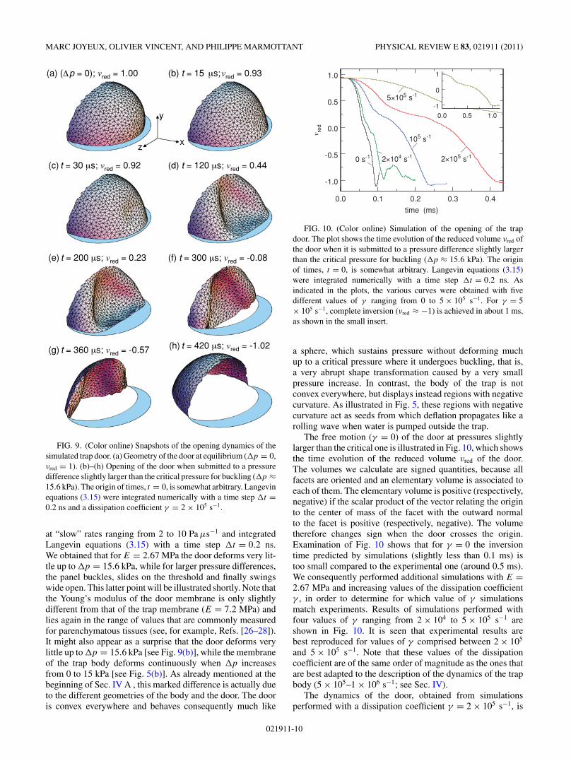
FIG. 9. (Color online) Snapshots of the opening dynamics of thesimulated trap door. (a) Geometry of the door at equilibrium (�p = 0,νred = 1). (b)–(h) Opening of the door when submitted to a pressuredifference slightly larger than the critical pressure for buckling (�p ≈15.6 kPa). The origin of times, t = 0, is somewhat arbitrary. Langevinequations (3.15) were integrated numerically with a time step �t =0.2 ns and a dissipation coefficient γ = 2 × 105 s−1.

at “slow” rates ranging from 2 to 10 Pa μs−1 and integratedLangevin equations (3.15) with a time step �t = 0.2 ns.We obtained that for E = 2.67 MPa the door deforms very lit-tle up to �p = 15.6 kPa, while for larger pressure differences,the panel buckles, slides on the threshold and finally swingswide open. This latter point will be illustrated shortly. Note thatthe Young’s modulus of the door membrane is only slightlydifferent from that of the trap membrane (E = 7.2 MPa) andlies again in the range of values that are commonly measuredfor parenchymatous tissues (see, for example, Refs. [26–28]).It might also appear as a surprise that the door deforms verylittle up to �p = 15.6 kPa [see Fig. 9(b)], while the membraneof the trap body deforms continuously when �p increasesfrom 0 to 15 kPa [see Fig. 5(b)]. As already mentioned at thebeginning of Sec. IV A , this marked difference is actually dueto the different geometries of the body and the door. The dooris convex everywhere and behaves consequently much like

0.0 0.1 0.2 0.3 0.4

-1.0

-0.5

0.0

0.5

1.0

time (ms)

2×104 s-10 s-1 2×105 s-1

105 s-1v red

5×105 s-1

0.0 0.5 1.0-1

0

1

FIG. 10. (Color online) Simulation of the opening of the trapdoor. The plot shows the time evolution of the reduced volume νred ofthe door when it is submitted to a pressure difference slightly largerthan the critical pressure for buckling (�p ≈ 15.6 kPa). The originof times, t = 0, is somewhat arbitrary. Langevin equations (3.15)were integrated numerically with a time step �t = 0.2 ns. Asindicated in the plots, the various curves were obtained with fivedifferent values of γ ranging from 0 to 5 × 105 s−1. For γ = 5× 105 s−1, complete inversion (νred ≈ −1) is achieved in about 1 ms,as shown in the small insert.

a sphere, which sustains pressure without deforming muchup to a critical pressure where it undergoes buckling, that is,a very abrupt shape transformation caused by a very smallpressure increase. In contrast, the body of the trap is notconvex everywhere, but displays instead regions with negativecurvature. As illustrated in Fig. 5, these regions with negativecurvature act as seeds from which deflation propagates like arolling wave when water is pumped outside the trap.

The free motion (γ = 0) of the door at pressures slightlylarger than the critical one is illustrated in Fig. 10, which showsthe time evolution of the reduced volume νred of the door.The volumes we calculate are signed quantities, because allfacets are oriented and an elementary volume is associated toeach of them. The elementary volume is positive (respectively,negative) if the scalar product of the vector relating the originto the center of mass of the facet with the outward normalto the facet is positive (respectively, negative). The volumetherefore changes sign when the door crosses the origin.Examination of Fig. 10 shows that for γ = 0 the inversiontime predicted by simulations (slightly less than 0.1 ms) istoo small compared to the experimental one (around 0.5 ms).We consequently performed additional simulations with E =2.67 MPa and increasing values of the dissipation coefficientγ , in order to determine for which value of γ simulationsmatch experiments. Results of simulations performed withfour values of γ ranging from 2 × 104 to 5 × 105 s−1 areshown in Fig. 10. It is seen that experimental results arebest reproduced for values of γ comprised between 2 × 105

and 5 × 105 s−1. Note that these values of the dissipationcoefficient are of the same order of magnitude as the ones thatare best adapted to the description of the dynamics of the trapbody (5 × 105–1 × 106 s−1; see Sec. IV).

The dynamics of the door, obtained from simulationsperformed with a dissipation coefficient γ = 2 × 105 s−1, is

021911-10

MECHANICAL MODEL OF THE ULTRAFAST UNDERWATER . . . PHYSICAL REVIEW E 83, 021911 (2011)

illustrated further in Figs. 9(b)–9(h). Figure 9(b) shows thegeometry of the door for a pressure difference �p slightlylarger than 15.6 kPa, just before the onset of buckling.Comparison of Figs. 9(a) and 9(b) shows that the panel is onlyslightly deformed with respect to its equilibrium geometry at�p = 0. This is, of course, due to the fact that pressure forcesare balanced by the reaction of the threshold on the free edgeof the panel. Figure 9(c) shows the first indentation, whichappears close to the center of the panel, at the place wheretrigger hairs are fixed to the door in real Utricularia traps. It isworth mentioning that the fact that the first indentation occursin the xy plane is a consequence of the ellipsoid geometry ofthe door. When modeling the door as a quarter of a sphereinstead of a quarter of an ellipsoid, one indeed observes twosymmetrical indentations on the sides of the panel, instead of asingle one at the center. In excellent agreement with high-speedvideos (see Fig. 8), the inversion of curvature then spreadsover the panel in about 0.1 ms, but the door is still closed[Fig. 9(d)]. At that point, the surface of the panel, which isflattened against the threshold by pressure forces, is draggedacross the threshold. This is certainly the step of the openingsequence that depends most on the precise geometry of thedoor. As can be checked in Fig. 10, it corresponds to a decreaseof the speed of evolution of νred. The duration of this step can,however, be substantially modified by changing the width ofthe threshold and/or its inclination with respect to the xz plane.The surface of the panel flattened against the threshold bypressure forces is also smaller (and the drag time shorter) ifthe door is not modeled as a quarter of an ellipsoid, but ratheras a smaller portion thereof, like, for example, a sixth or aneighth of an ellipsoid. For some geometries, the only part ofthe panel which is ever in contact with the threshold is itsfree (lower) edge, which simply slides on the threshold. Atlast, let us recall that in real Utricalaria traps this dragging orsliding motion across the threshold is slowed down by frictionforces, which we neglect in our simulations. It is only when thefree edge of the panel reaches the inner side of the threshold[Fig. 9(e)] that the door really opens and water enters the trap.Inversion of the door then proceeds freely [Figs. 9(f) and 9(g)]until complete inversion is attained [Fig. 9(h)]. Comparisonof Figs. 8 and 9 shows that the door profiles during openingobtained with the membrane model agree qualitatively withthe observed ones.

Complete inversion corresponds to a stable equilibriumin our simulations, because we assumed that the differencebetween pressure forces exerted on the external and internalsides of the membrane is constant. In real Utricularia traps,this pressure difference, however, decreases as water entersthe trap and finally vanishes. When pressures are leveled,the door again closes autonomously in about 2.5 ms. Ourhigh-speed video recordings show that closure of the doorproceeds through the same steps as opening, but of course inreverse order. We made no attempt to simulate this last step ofthe opening and closure door mechanism.

In our simulations, the opening mechanism is fired byincreasing slowly �p above the critical pressure for buckling(�p ≈ 15.6 kPa). In real Utricularia traps, the pressuredifference �p remains instead almost constant once the trapis set, and the mechanism is fired by potential prey touchingthe trigger hairs. The question of whether triggering is purely

0.00 0.02 0.04 0.06 0.08 0.10 0.12

-30

-20

-10

0

10

20

1 - vred

15.6 kPa

Ereact

10 kPa

5 kPa

Ere

act -

Δp

v 0 (

1-v re

d)

(nJ

)

20 kPa

25 kPa

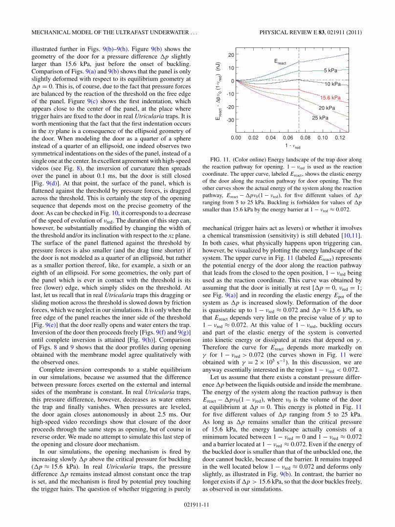
FIG. 11. (Color online) Energy landscape of the trap door alongthe reaction pathway for opening. 1 − νred is used as the reactioncoordinate. The upper curve, labeled Ereact, shows the elastic energyof the door along the reaction pathway for door opening. The fiveother curves show the actual energy of the system along the reactionpathway, Ereact − �pν0(1 − νred), for five different values of �p

ranging from 5 to 25 kPa. Buckling is forbidden for values of �p

smaller than 15.6 kPa by the energy barrier at 1 − νred ≈ 0.072.

mechanical (trigger hairs act as levers) or whether it involvesa chemical transmission (sensitivity) is still debated [10,11].In both cases, what physically happens upon triggering can,however, be visualized by plotting the energy landscape of thesystem. The upper curve in Fig. 11 (labeled Ereact) representsthe potential energy of the door along the reaction pathwaythat leads from the closed to the open position, 1 − νred beingused as the reaction coordinate. This curve was obtained byassuming that the door is initially at rest [�p = 0, νred = 1;see Fig. 9(a)] and in recording the elastic energy Epot of thesystem as �p is increased slowly. Deformation of the dooris quasistatic up to 1 − νred ≈ 0.072 and �p ≈ 15.6 kPa, sothat Ereact depends very little on the precise value of γ up to1 − νred ≈ 0.072. At this value of 1 − νred, buckling occursand part of the elastic energy of the system is convertedinto kinetic energy or dissipated at rates that depend on γ .Therefore the curve for Ereact depends more markedly onγ for 1 − νred > 0.072 (the curves shown in Fig. 11 wereobtained with γ = 2 × 105 s−1). In this discussion, we areanyway essentially interested in the region 1 − νred < 0.072.

Let us assume that there exists a constant pressure differ-ence �p between the liquids outside and inside the membrane.The energy of the system along the reaction pathway is thenEreact − �pν0(1 − νred), where ν0 is the volume of the doorat equilibrium at �p = 0. This energy is plotted in Fig. 11for five different values of �p ranging from 5 to 25 kPa.As long as �p remains smaller than the critical pressureof 15.6 kPa, the energy landscape actually consists of aminimum located between 1 − νred = 0 and 1 − νred ≈ 0.072and a barrier located at 1 − νred ≈ 0.072. Even if the energy ofthe buckled door is smaller than that of the unbuckled one, thedoor cannot buckle, because of the barrier. It remains trappedin the well located below 1 − νred ≈ 0.072 and deforms onlyslightly, as illustrated in Fig. 9(b). In contrast, the barrier nolonger exists if �p > 15.6 kPa, so that the door buckles freely,as observed in our simulations.

021911-11

MARC JOYEUX, OLIVIER VINCENT, AND PHILIPPE MARMOTTANT PHYSICAL REVIEW E 83, 021911 (2011)

In real Utricularia traps, the pressure difference �p inset conditions is probably only very slightly smaller than thecritical pressure for buckling. This implies that the barrierhindering buckling along the reaction pathway is very small,too. In this case, the torsion exerted on the membrane whentrigger hairs are touched by a potential prey may be sufficientto give the system that tiny amount of extra energy it needs toovercome the barrier and buckle. On the contrary, if chemicaltransmission (sensitivity) is involved instead of mechanicalaction [10,11], then the local bending and stretching energyconstants of the membrane are temporarily reduced when thetrigger hairs are touched. This has the effect of lowering thebarrier and letting the door buckle.

VI. CONCLUSION

The underwater traps of Utricularia carnivorous plantscatch their prey through the repetition of an active slowdeflation followed by passive fast suction sequence. In thispaper, we presented experimental results and theoreticalmodels aimed at understanding this mechanism. We firstshowed that a very simple disks-and-spring model enablesus to extract important information from the experimentalresults, like the maximum pumping rate, the characteristicpumping time, the hydraulic permeability of the membrane,the average elastic energy stored in the membrane, and themaximum velocity of the fluid during the suction phase. Wethen proposed a more elaborate model that describes thesecond step of this sequence, that is, the ultrafast suctionphase. This model consists of a thin membrane with strain andcurvature energy. The only free parameter in the expression ofthe elastic energy, the Young’s modulus E of the membrane,

is adjusted by requiring that the pressure difference betweenthe outside and the inside of the traps is close to measuredvalues (10–20 kPa) in set conditions. Obtained values of E(2–10 MPa) lie in the range of values that are commonlymeasured for parenchymatous tissues. The door of the trapis modeled as a quarter of an ellipsoid, one edge of which isfixed, while the other one is free and rests on the threshold in setconditions. Our simulations show that, for a pressure differenceslightly larger than the critical one, the door buckles, slides onthe threshold, and finally swings wide open. This sequence isin excellent agreement with that observed in high-speed videos(Fig. 8).

This model therefore strongly supports the hypothesis thatwe formulated by looking at the high-speed videos, that is, thatthe trap acts as a flexible valve that buckles under the combinedeffects of pressure forces and the mechanical stimulation oftrigger hairs, and not as a panel articulated on hinges. The onlyreal limitation of this model is that the liquid is only roughlytaken into account through the dissipation coefficient γ inLangevin equations. It was shown that γ must be chosen in therange 2 × 105–1 × 106 s−1 in order for the characteristic timesof the model to match observed ones. A better model wouldconsist in taking water explicitly into account and in integratingcoupled equations for the dynamics of the liquid and themembrane. This is, however, a much more complex problem.

To conclude, let us note that this work on the underwaterultrafast traps of Utricularia opens very interesting perspec-tives for the practical design of flexible structures performingfast motion in a fluid. Since such flexible structures show lessfatigue than articulated ones, the mechanism of the tiny trapsof Utricularia suggests a new kind of microfluidic tools, basedon buckling, for lab-on-chip devices.

[1] D. Attenborough, The Private Life of Plants (PrincetonUniversity Press, Princeton, 1995).

[2] L. Gaume and Y. Forterre, PLoS ONE 2, e1185 (2007).[3] Y. Forterre, J. M. Skotheim, J. Dumais, and L. Mahadevan,

Nature (London) 433, 421 (2005).[4] B. E. Juniper, R. J. Robins, and D. M. Joel, The Carnivorous

Plants (Academic, London, 1989).[5] F. E. Lloyd, The Carnivorous Plants (Chronica Botanica,

Waltham, MA, 1942).[6] A. T. Czaja, Z. Bot. 14, 705 (1922).[7] T. Ekambaram, J. Ind. Bot. Soc. 4, 73 (1924).[8] F. E. Lloyd, Can. J. Bot. 10, 780 (1932).[9] F. E. Lloyd, Plant Physiol. 4, 87 (1929).

[10] T. Diannelidis and K. Umrath, Protoplasma 42, 58 (1953).[11] P. Sydenham and G. Findlay, Australian J. Biol. Sci. 26, 1115

(1973).[12] C. L. Withycombe, J. Linn. Soc. 46, 401 (1924).[13] A. Sasago and T. Sibaoka, Bot. Mag. Tokyo 98, 55 (1985).[14] A. Sasago and T. Sibaoka, Bot. Mag. Tokyo 98, 113

(1985).[15] P. Taylor, The Genus Utricularia: A Taxonomic Monograph

(Kew Bulletin Additional Series XIV, London, 1989).[16] K. Reifenrath, I. Theisen, J. Schnitzler, S. Porembski, and

W. Barthlott, Flora 201, 597 (2006).

[17] O. Vincent, C. Weisskopf, S. Poppinga, T. Masselter, T. Speck,M. Joyeux, C. Quilliet, and P. Marmottant, Proc. Roy. Soc. B (inpress).

[18] J. M. Skotheim and L. Mahadevan, Science 308, 1308(2005).

[19] Introduction to Particle Technology, edited by M. Rhodes(Wiley, Weinheim, 1998).

[20] F. I. Niordson, Shell Theory (North-Holland, New York, 1985).[21] S. Komura, K. Tamura, and T. Kato, Eur. Phys. J. E 18, 343

(2005).[22] A. F. Bower, Applied Mechanics of Solids (CRC, Boca Raton,

2009).[23] M. Meyer, M. Desbrun, P. Schroder, and A. H. Barr, in

Visualization and Mathematics III, edited by H. C. Hege andK. Polthier (Springer, Heidelberg, 2003), pp. 35–57.

[24] J. Yong, B. Deng, F. Cheng, B. Wang, K. Wu, and H. Gu, Sci.China Ser. F: Inf. Sci. 52, 418 (2009).

[25] E. Magid, O. Soldea, and E. Rivlin, Computer Vision and ImageUnderstanding 107, 139 (2007).

[26] H. Alizadeh and L. J. Segerlind, Applied Engineering inAgriculture 13, 507 (1997).

[27] L. Mayor, R. L. Cunha, and A. M. Sereno, Food ResearchInternational 40, 448 (2007).

[28] K. J. Niklas, Am. J. Bot. 75, 1286 (1988).

021911-12