How to Measure Quality of Credit Scoring Models

Martin Řezáč,

Dept. of Mathematics and Statistics, Faculty of Science, Masaryk University, Kotlářská 2, 611 37 Brno, Czech Republic, mrezac@math.muni.cz

František Řezáč, Dept. of Finance, Faculty of Economics and Administration, Masaryk University, Lipová

41a, 602 00 Brno, Czech Republic, rezac@econ.muni.cz

Abstract Credit scoring models are widely used to predict a probability of client’s default. To measure the quality of the scoring models it is possible to use quantitative indexes such as Gini index, K-S statistics, Lift, Mahalanobis distance and Information statistics. They are used for comparison of several developed models at the moment of development as well as for monitoring of quality of those models after deployment into real business. The paper deals with definition of good/bad client, which is crucial for further computations. Parameters affecting this definition are discussed. The main part is devoted to quality indexes based on distribution functions (Gini, K-S and Lift) and on density functions (Mahalanobis distance, Information statistics). It brings some interesting results connected to the Lift, especially the expression of the Lift by cumulative distribution functions of scores of bad and all clients, which allows computing value of the Lift for any level of score. Kernel density estimates are used in case of density based indexes, namely for the Information statistics. We extend some known results for normally distributed scores, especially in general case of unequal variances of scores. All proposed expressions are discussed and illustrated in appropriate figures. Over all, application of all listed quality indexes, including appropriate computation issues, is illustrated in the case study based on real financial data.

JEL Classification: C10, C53, D81, G32 Keywords: Credit scoring, Quality indexes, Distribution function, Density function, Normally distributed scores

1. Introduction

Banks and other financial institutions receive thousands of credit applications every day

(in case of consumer credits it can be tens or hundreds of thousands every day). Since it is impossible to process them manually, automatic systems are widely used by these institutions for evaluating credit reliability of individuals who ask for credit. The assessment of the risk associated with granting of credits has been underpinned by one of the most successful applications of statistics and operations research: credit scoring.

Credit scoring is the set of predictive models and their underlying techniques that aid financial institutions in the granting of credits. These techniques decide who will get credit, how much credit they should get, and what further strategies will enhance the profitability of the borrowers to the lenders. Credit scoring techniques assess the risk in lending to a

particular client. They do not identify “good” or “bad” (negative behaviour is expected, e.g. default) applications on an individual basis, but they forecast probability, that an applicant with any given score will be “good” or “bad”. These probabilities or scores, along with other business considerations such as expected approval rates, profit, churn, and losses, are then used as a basis for decision making.

Several modelling methods for credit scoring have been introduced during the last six decades. The best known and most widely used are logistic regression, classification trees, linear programming approach and neural networks.

It is impossible to use scoring model effectively without knowing how good it is. First, one needs to select the best model with regard to some measure of quality at the time of development. Second, one needs to monitor the quality after deployment into real business. Methodology of credit scoring models and some measures of their quality were discussed in surveys like Hand and Henley (1997), Thomas (2000) or Crook at al. (2007). Even ten years ago a list of really good books devoted to the issue of credit scoring was not large. The situation has improved in the last decade. For instance, books such as Anderson (2007), Crook et al. (2007), Siddiqi (2006), Thomas et al. (2002) and Thomas (2009) were published. Further remarks connected to credit scoring issues can be found there as well.

Despite the fact, that there are some books and articles in scientific journals, there is no comprehensive work devoted to assessment of credit scoring model’s quality in the full complexity. Due to that, we decided to summarize and extend known results on this topic. From the definition of good/bad client through the list of the most popular indexes to their expressions for normally distributed scores, generally with unequal variances of scores.

The most used indexes in practice are Gini index, number one in Europe, and KS, number one in North America. Despite the fact, that their use may not be optimal. It is obvious that we need to have the best performance of given scoring model nearby expected cutoff value. Hence we should judge quality indexes from this point of view. Gini index is global measure, hence it is impossible to use it for assessment of local quality. The same holds for mean difference D. The KS is ideal if the expected cutoff value is near that point where KS is realized. Although the information statistics is global measure of model’s quality, we propose to use graphs of difff , LRf and graph of their product to examine local properties of given model. Especially we can focus on region of scores where the cutoff is expected. Overall, the Lift seems to be the best choice for our purpose. Since we proposed expression of the Lift by cumulative distribution functions of scores of bad and all clients, it is possible to compute the value of the Lift for any level of score.

The contribution of this paper to practice is the comprehensive overview of widely used techniques of assessment of credit scoring model’s quality, including appropriate discussion. Firstly we discuss definition of good/bad client, which is crucial for further computation. Result of quality assessment process really highly depends on this definition. In the next section we review widely used quality indexes, their properties and mutual relationships and extend some results connected to them. Furthermore we extend known results for normally distributed scores. Finally, application of all listed quality indexes, including appropriate computation issues, is illustrated in the case study based on real financial data.

The main contribution to the theory is the expression of the Lift by cumulative distribution functions of scores of bad and all clients and expressions of selected indexes for normally distributed data. Namely, Gini index and Lift in case of common variance of scores and mean difference D, KS, Gini index, Lift and Information statistics in general case, i.e. without assumption of equality of variances.

2. Definition of good/bad client In fact, the most important step in predictive model building is the correct definition of

dependent variable. In case of credit scoring it is necessary to precisely define good and bad client. Usually this definition is based on the client’s number of days after the due date (days past due, DPD) and the amount past due. We need to set some tolerance level in case of the past due amount. It means what it is considered as the debt and what is not. It may be that the client gets into payment delay innocently (because of technical imperfections of the system). It does not make sense to regard as debt small amount (e.g. less than 3€) past due as well. Furthermore, it is necessary to determine the time horizon in which the previous two characteristics are traced. For example, as a good is marked client who: Has less than 60 DPD (with tolerance 3€) in 6 months from the first due date Has less than 90 DPD (with tolerance 1€) ever

Choice of these parameters depends greatly on the type of financial product (certainly will be different parameters for consumer loans for small amounts with original maturities around one year and for mortgages, which are typically connected to very large amounts with maturities up to several tens of years) and on further usage of this definition (credit scoring, fraud prevention, marketing, ...). Another practical issue of the definition of good client is the accumulation of several agreements. For example, it may be that the customer is overdue on more contracts, but with different days past due and with different amounts. In this case, all amounts past due connected to the client in one particular point in time are usually added together and it is taken the maximum value from days past due. This approach can be applied only in some cases and especially in a situation where there is a complete accounting data. The situation is considerably more complex in case of aggregated data.

In connection with the definition of good client we can generally talk about the following types of clients: Good Bad Indeterminate Insufficient Excluded Rejected.

The first two types were discussed. The third type of client is on the border between good and bad clients, and directly affects their definition. If we are considering only DPD, clients with a high DPD (e.g. 90 +) are typically identified as bad, clients who are not delinquent (e.g. their DPD are less than 30 or equal to zero) are identified as good. As indeterminate are then considered delinquent customers who have not exceeded given threshold of DPD. When we use this type of clients, then we model very good clients against very bad ones. Consequence is obtaining a model with amazing predictive power. Indeed, this power dive immediately after assessing the model on whole population, where indeterminates are considered to be good. Thus the usage of this type of clients is very disputable and usually does not lead to any improvement of model’s quality. The next type is typically case of the clients with the very short history, which makes impossible the correct definition of dependent variable (good / bad client). The excluded clients are typically clients with so wrong data as to be misleading (e.g. frauds). They are also marked as “hard bad”. The second group of excluded clients consists of applicants who belong to a category that will not be assessed by a model (scorecard), e.g.

VIPs. The meaning of rejected client is obvious. See Anderson (2007), Thomas et al. (2002) or Thomas (2009) for more details.

Only good and bad clients are used for further model building. When we do not use indeterminate category, set up some tolerance level for amount past due and solve somehow the issue with simultaneous contracts, it remains two parameters affecting the good/bad definition. It is DPD and time horizon. Usually it is useful to build up set of models with varying levels of these parameters. Furthermore it can be useful to develop a model with one good/bad definition and measure the model’s quality with another. It should hold that scoring models developed on harder definition (higher DPD, longer time horizon or measuring DPD on first payment) perform better than those developed on softer definitions (Witzany 2009). Furthermore, it should hold that given scoring model has higher performance if it is measured by harder good/bad definition. If not, usually it means that something is wrong. Over all, development and assessment of credit scoring models on as hard as possible and reasonable definition should lead to the best performance. 3. Measuring the quality

Once the definition of good / bad client and client's score is available, it is possible to evaluate the quality of this score. If the score is an output of a predictive model (scoring function), then we evaluate the quality of this model. We can consider two basic types of quality indexes. First, indexes based on cumulative distribution function like Kolmogorov-Smirnov statistics, Gini index and Lift. The second, indexes based on likelihood density function like Mean difference (Mahalanobis distance) and Informational statistics. For further available measures and appropriate remarks see Wilkie (2004), Giudici (2003) or Siddiqi (2006). 3.1. Indexes based on distribution function

Assume that score s is available for each client and put the following markings.

=.,0

,1otherwise

goodisclientDK

Empirical cumulative distribution functions (CDF) of scores of good (bad) clients are given by the relationships

( )11)(1

. =∧≤= ∑=

Ki

n

iGOODn DasI

naF , (1)

( )01)(1

. =∧≤= ∑=

Ki

m

iBADm DasI

maF , [ ]HLa ,∈ , (2)

where is is score of ith client, n is number of good, m is number of bad clients and I is the indicator function where I(true)=1 and I(false)=0. L is the minimum value of given score, H is the maximum value. The proportion of bad clients we denote by

mnmpB +

= ,

proportion of good clients by

mnnpG +

= .

Furthermore, empirical distribution function of scores of all clients is given by

( )asIN

aF i

N

iALLN ≤= ∑

=1.

1)( , [ ]HLa ,∈ , (3)

where mnN += is number of all clients.

An often-used characteristic in describing the quality of the model (scoring function) is Kolmogorov-Smirnov statistics (K-S or KS). It is defined as

[ ])()(max ,,,

aFaFKS GOODnBADmHLa−=

∈. (4)

Figure 1 gives an example of estimation of distribution functions of good and bad clients, including an estimate of KS statistics. It can be seen, for example, that the score around 2.5 and smaller has population of approximately 30% of good clients and 70% of bad clients.

Figure 1: Distribution Functions, KS.

The Lorenz curve (LC), sometimes confused with ROC curve (Receiver Operating

Characteristic curve), can also be successfully used to show the discriminatory power of scoring function, i.e. the ability to identify good and bad clients. The curve is given parametrically by

[ ].,),()(

.

.

HLaaFyaFx

GOODn

BADm

∈==

The definition and name (LC) is consistent with Müller, M., Rönz, B. (2000). The same definition of the curve, but called ROC one can find in Thomas et al. (2002). Siddiqi (2006) used name ROC for curve with reversed axes and LC for curve with CDF of bad clients on vertical axis and CDF of all clients on horizontal axis.

Each point of curve represents some value of given score. If we assume this value as cutoff value, we can read the proportion of rejected bad and good clients. An example of Lorenz curve is given in Figure 2. We can see that by rejection of 20% of good clients we reject almost 60% of bad clients at the same moment.

Figure 2: Lorenz Curve, Gini index.

In connection to LC we consider next quality measure, Gini index. This index describes a

global quality of scoring function. It takes values between -1 and 1. The ideal model, i.e. scoring function that perfectly separate good and bad clients, has the Gini index equal to 1. On the other hand, model that assigns a random score to the client has this index equal to 0. Negative values correspond to a model with reversed meaning of scores. Using Figure 2 it can be defined as

ABA

AGini 2=+

= .

The actual calculation of Gini index can be, given the previous markings, made using

( )[ ( )]1..2

1..1 −

+

=− +⋅−−= ∑ kGOODnGOODn

mn

kkBADmkBADm FFFFGini

k, (5)

where kBADmF . (

kGOODnF . ) is kth vector value of empirical distribution function of bad (good) clients. For further details see Thomas et al. (2002), Siddiqi (2006) or Xu (2003).

The Gini index is a special case of Somers’ D (Somers (1962)), which is an ordinal association measure defined in general as

XX

XYYXD

ττ

= ,

where XYτ is Kendall’s aτ defined as

( ) ( )[ ]2121 YYsignXXsignEXY −−=τ , where ( )11 ,YX , ( )22 ,YX are bivariate random variables sampled independently from the same population, and [ ]⋅E denotes expectation. In our case, 1=X if a client was good and 0=X if the client was bad. Variable Yrepresents scores. It can be found in Thomas (2009), that Somers’ D assessing performance of given credit scoring model, denoted as SD , one can calculate as

mn

bgbgD ij

ji

iij

ji

i

S ⋅

−=

∑∑∑∑>< , (6)

FBAD F G

OO

D

where ig ( jb ) is number of goods (bads) in ith interval of scores. Furthermore it holds that

SD can be expressed by Mann-Whitney U-statistic in following way. Order the sample in increasing order of score and sum ranks of goods in the sequence. Let this be GR . The SD is then given by

12 −⋅

=mn

UDS , (7)

where U is given by

( )121

+−= nnRU G . (8)

Some further details can be found in Nelsen (1998).

Another available type of quality assessment figure is CAP (Cumulative Accuracy Profile). Another names used for this concept are Lift chart, Lift curve, Power curve or Dubbed curve. See Sobehart et al. (2000) or Thomas (2009) for more details.

In this case we have the proportion of all clients (FALL) on the horizontal axis and the proportion of bad clients (FBAD) on the vertical axis. An example of Lift chart is displayed in Figure 4. The ideal model is now represented by polyline from [0, 0] through [pB, 1] to [1, 1]. Advantage of this figure is that one can easily read the proportion of rejected bads vs. proportion of all rejected. For example in case of Figure 3 we can see that if we want to reject 70% of bads, we have to reject about 40% of all applicants.

Figure 3: CAP.

It is called Gains chart in case of marketing usage, see Berry and Linoff (2004). In this case, the horizontal axis represents proportion of clients who can be addressed by some marketing offer and the vertical axis represents proportion of clients who will accept the offer.

When we use CAP instead of LC, we can define the Accuracy Rate (AR), see Thomas (2009). Again, it is defined by ratio of some areas. We have

Although the ROC and CAP are not equvivalent, it is true that Gini index and AR are equal for any scoring model. Proof for discrete scores is given in Engelmann et al. (2003), for continuous scores one can find it in Thomas (2009).

In connection to the Gini index, c-statistics (Siddiqi 2006) is defined as

21 Ginistatc +

=− . (9)

It represents the likelihood that randomly selected good client has higher score than randomly selected bad client, i.e.

( )012121 =∧=≥=− KK DDssPstatc .

It takes values from 0.5, for random model, to 1, for ideal model. Another name for c-statistic can be found in literature. It is Harrell's c, which is a reparameterization of Somers' D and is recommended in Harrell et al. (1996) as a general measure of the predictive power of a prognostic score arising from a medical test. Further details can be found in (Newson 2006). Furthermore it is called AUROC, e.g. in Thomas (2009) or AUC, e.g. in Engelmann et al. (2003).

Another possible indicator of the quality of scoring model can be cumulative Lift, which says, how many times, at a given level of rejection, is the scoring model better than random selection (random model). More precisely, the ratio indicates the proportion of bad clients with less than a score a, [ ]HLa ,∈ , to the proportion of bad clients in the general population. Formally, it can be expressed by

( )

( )

( )

( )

( )

( )

Nn

asI

DasI

DDI

DI

asI

DasI

BadRateaBadRateaLift

i

n

i

Ki

n

i

KK

mn

i

K

n

i

i

n

i

Ki

n

i

≤

=∧≤

=

=∨=

=

≤

=∧≤

==∑

∑

∑

∑

∑

∑

=

=

+

=

=

=

=

1

1

1

1

1

10

10

0

0

)()(

It can be easily verified that the Lift can be equivalently expressed as

)()(

)(.

.

aFaF

aLiftALLN

BADn= , [ ]HLa ,∈ . (10)

In practice, this calculation is done for Lift corresponding to 10%, 20%, ..., 100% of clients with the worst score. Let’s demonstrate this procedure by the following example, taken from Coppock (2002). Assume that we have a score of 1000 clients, of which 50 are bad. The proportion of bad clients is 5%. Sort customers according to score and split into ten groups, i.e., divide it by deciles of score. In each group, in our case around 100 clients, then count bad clients. This will get their share in the group (Bad Rate). Absolute Lift in each group is then given by the ratio of the share of bad clients in the group to the proportion of bad clients in total. Cumulative Lift is given by the ratio of the share of bad clients in groups up to the given group to the proportion of bad clients in total. See Table 1.

Table 1: Absolute and Cumulative Lift # bad clients Bad rate abs. Lift # bad clients Bad rate cum. Lift

1 100 16 16,0% 3,20 16 16,0% 3,20 2 100 12 12,0% 2,40 28 14,0% 2,80 3 100 8 8,0% 1,60 36 12,0% 2,40 4 100 5 5,0% 1,00 41 10,3% 2,05 5 100 3 3,0% 0,60 44 8,8% 1,76 6 100 2 2,0% 0,40 46 7,7% 1,53 7 100 1 1,0% 0,20 47 6,7% 1,34 8 100 1 1,0% 0,20 48 6,0% 1,20 9 100 1 1,0% 0,20 49 5,4% 1,09

10 100 1 1,0% 0,20 50 5,0% 1,00 All 1000 50 5,0%

absolutely cumulativelydecile # cleints

In connection to the previous example we define

( ))(1))(())(( 1

..1..

1.. qFF

qqFFqFFLift ALLNBADn

ALLNALLN

ALLNBADnq

−−

−

== , (11)

where q represents the score level of 100q% of the worst scores and )(1

. qF ALLN− can be

computed as { }qaFHLaqF ALLNALLN ≥∈=− )(],,[min)( .

1. .

Since the expected reject rate is usually between 5% and 20%, q is typically assumed to be equal 0.1 (10%), i.e. we are interested in discriminatory power of scoring model in point of 10% of the worst scores. In this case we have

( ).)1.0(10 1..%10−⋅= ALLNBADn FFLift .

3.2. Indexes based on density function

Let gM and bM be means of scores of good (bad), clients and gS and bS be standard deviations of good (bad) clients. Let S be the pooled standard deviation of the good and bad clients given by

21

22

+

+=

mnmSnS

S bg .

Estimates of mean and standard deviation of scores for all clients ( ALLALL σµ , ) are given by

mnmMnM

MM bgALL +

+== ,

( ) ( )( )

21

2222

+

−+−++=

mnMMmMMnmSnS

S bgbgALL .

The first quality index based on density function is the standardized difference between the means of two groups of scores, i.e. scores of bad and good clients. Denote by D this mean difference, calculated as

SMM

D bg −= .

Generally, good clients are supposed to get high scores and bad clients low scores, so that we would expect that bg MM > , so that D is positive. Another name for this concept is Mahalanobis distance; see Thomas et al. (2002).

The second index based on densities is the information statistics (value) valI , defined in Hand and Henley (1997) as

( ) dxxfxfxfxfI

BAD

GOODBADGOODval

−= ∫

∞

∞− )()(

ln)()( . (12)

We propose to examine decomposed form of right-hand side expression. For this purpose we mark

)()( xfxff BADGOODdiff −= ,

=

)()(

lnxfxf

fBAD

GOODLR .

Although the information statistics is global measure of model’s quality, one can use graphs of difff , LRf and graph of their product to examine local properties of given model, see section 4 for more details.

We have two basic ways how to compute the value of this index. First way is to create bins of scores and compute it empirically from a table with counts of good and bad clients in that bins. The second way is to estimate unknown densities using kernel smoothing theory. Consequently we compute the integral by a suitable numerical method.

Let’s have m score value mis i ,...,1,,0 = for bad clients and n score values njs j ,...,1,,1 = for good clients and recall that L denotes the minimum of all values and H the

maximum. Let’s divide the interval [L,H] to r equal subinterval [q0, q1], (q1, q2],…(qr-1, qr], where q0 = L, qr = H. Set

rkqqsIn

qqsIn

n

jkkjk

m

ikkik

,...,1,)],((

)],((

11,1,1

11,0,0

=∈=

∈=

∑

∑

=−

=−

observed counts of bad and good in each interval. Then the empirical information value is calculated by

∑=

⋅

⋅

−=

r

k k

kkkval nn

mnm

nn

nI

1 ,0

,1,0,1 ln . (13)

The following Table 2 gives an example of computational scheme for informational statistics in case of discretized data. Table 2: Informational Statistics

score int. # bad clients #good clients % bad [1] % good [2] [3] = [2] - [1] [4] = [2] / [1] [5] = ln[4] [6] = [3] * [5]1 1 10 2,0% 1,1% -0,01 0,53 -0,64 0,012 2 15 4,0% 1,6% -0,02 0,39 -0,93 0,023 8 52 16,0% 5,5% -0,11 0,34 -1,07 0,114 14 93 28,0% 9,8% -0,18 0,35 -1,05 0,195 10 146 20,0% 15,4% -0,05 0,77 -0,26 0,016 6 247 12,0% 26,0% 0,14 2,17 0,77 0,117 4 137 8,0% 14,4% 0,06 1,80 0,59 0,048 3 105 6,0% 11,1% 0,05 1,84 0,61 0,039 1 97 2,0% 10,2% 0,08 5,11 1,63 0,13

10 1 48 2,0% 5,1% 0,03 2,53 0,93 0,03All 50 950 Info. Value 0,68

Second and third column contain counts of bad and good clients. Next two columns, [1] and [2], contain relative frequencies of bad and good clients in each score interval. Last four columns, [3] to [6], represent mathematical operations employed in (13). Adding the last column [6] we get information value.

Another way how to compute this index is estimation of appropriate densities using kernel estimations. Consider )(xfGOOD and )(xfBAD to be likelihood density functions of scores of good or bad clients respectively. The kernel density estimates are defined by

( )∑=

−=n

jjhGOOD sxK

nhxf

1,11 1

1),(~ , ( )∑=

−=m

iihBAD sxK

nhxf

1,00 0

1),(~ ,

where

=

iih h

xKh

xKi

1)( , i= 0,1 and K is some kernel function, e.g. Epanechnikov kernel.

For further details see Wand and Jones (1995). The estimation of bandwidth hi can be given by maximal smoothing principal approach, see Terrel (1990) or Řezáč (2003), i.e.

12112

1

23

,~

)!32()52()!12( +

−++

⋅⋅

+++

= kkk

kOS nk

kkkh σ ,

where k is the order of kernel K, σ~ is an appropriate estimation of standard deviation and n is the number of observations.

As the next step we need to estimate the final integral. We use the composite trapezoidal rule. Set

( )

⋅−=

),(~),(~

ln),(~),(~)(~

0

101 hxf

hxfhxfhxfxfBAD

GOODBADGOODIV .

Then, for given M+1 equidistant points L = x0,…,xM = H we obtain

++

−= ∑

−

=

)(~)(~)(~2

1

1HfxfLf

MLHI IV

M

iiIVIVval . (14)

For further details see Koláček and Řezáč (2010). 3.3 Some results for normally distributed scores

Assume that the scores of good and bad clients are each approximately normally distributed, i.e. we can write their densities as

( )2

2

2

21)( g

gx

gGOOD exf σ

µ

πσ

−−

= ,

( )2

2

2

21)( b

bx

bBAD exf σ

µ

πσ

−−

= .

The values of gM , bM and gS , bS can be taken as estimates of gµ , bµ and gσ , bσ . Finally we assume that standard deviations are equal to a common value σ . In practice, this assumption should be tested by F-test.

The mean difference D (see Wilkie (2004)) is now defined as

σµµ bgD

−=

and is calculated by

SMM

D bg −= . (15)

The maximum difference between the cumulative distributions, denoted KS before, is calculated, as proposed in Wilkie (2004), at the point where the distributions cross, halfway between the means. The value KS is therefore given by

12

222

−

Φ⋅=

−Φ−

Φ=

DDDKS , (16)

where ( )⋅Φ is the standardized normal distribution function. We derived formula for Gini index. It can be expressed by

12

2 −

Φ⋅=

DG . (17)

For the Lift statistics is computation quite easy. Denoting )(1 ⋅Φ− the standard normal quantile function and )(2, ⋅Φ

σµ the normal distribution function with expected value µ and variance

2σ , we have

( )

⋅+Φ⋅Φ= − Dpq

qLift G

ALLq

11σ

σ .

Computational form is then

( )

⋅+ΦΦ= − Dpq

SS

qLift G

ALLq

11 . (18)

A couple of further interesting results are given in Wilkie (2004). One of them is that, under our assumptions on normality and equality of standard deviations, it holds

2DIval = . (19)

We derived expressions for all mentioned indexes in general case, i.e. without assumption of equality of variances. The mean difference is now in form

*2 DD = , (20)

where 22

*

bg

bgDσσ

µµ

+

−= .

The KS is given by

⋅+−⋅Φ−

⋅+−⋅Φ=

cbDab

Dba

cbDab

DbaKS

bg

gb

21

21

2

2

*2*

*2*

σσ

σσ,

where 22gba σσ += , ,22

gbb σσ −=

=

b

gcσσ

ln . Empirical form can be expressed by

( ) ( )

( ) ( ).

ln2

1

ln2

1

22*22

22*

22

22

22*22

22*

22

22

2

2

−⋅++⋅

⋅−

−⋅−

+

Φ−

−⋅++⋅

⋅−

−⋅−

+

Φ=

b

ggbgb

bgb

ggb

gb

b

ggbgb

ggb

bgb

gb

SS

SSDSS

SSS

DSSSSS

SS

SSDSS

SSS

DSSSSS

KS

(21)

Gini coefficient can be expressed as

( ) 12 * −Φ⋅= DG . (22) Lift is given by formula

( )( )

( )

−+Φ⋅Φ=

=Φ⋅+Φ=

−

−

b

bALLALL

ALLALLq

qq

qq

Liftbb

σµµσ

σµσµ

1

1,

1

12

.

When we replace theoretical means and standard deviations by their estimates we obtain

( )

−+Φ⋅Φ=

−

b

bALLq S

MMqSq

Lift11 . (23)

Finally, information statistics is given by

( ) 11 2* −++= ADAIval , (24)

where

+= 2

2

2

2

21

g

b

b

gAσσ

σσ

, in computation form it is

+= 2

2

2

2

21

g

b

b

g

SS

SS

A . For this index one can

find similar formula in Thomas (2009). Some of these results are graphically expressed in relation to bµ , gµ and 2

bσ , 2gσ in the

following figures. In case of Figures 4 to 7 it was selected 0=bµ , 12 =bσ . There is displayed

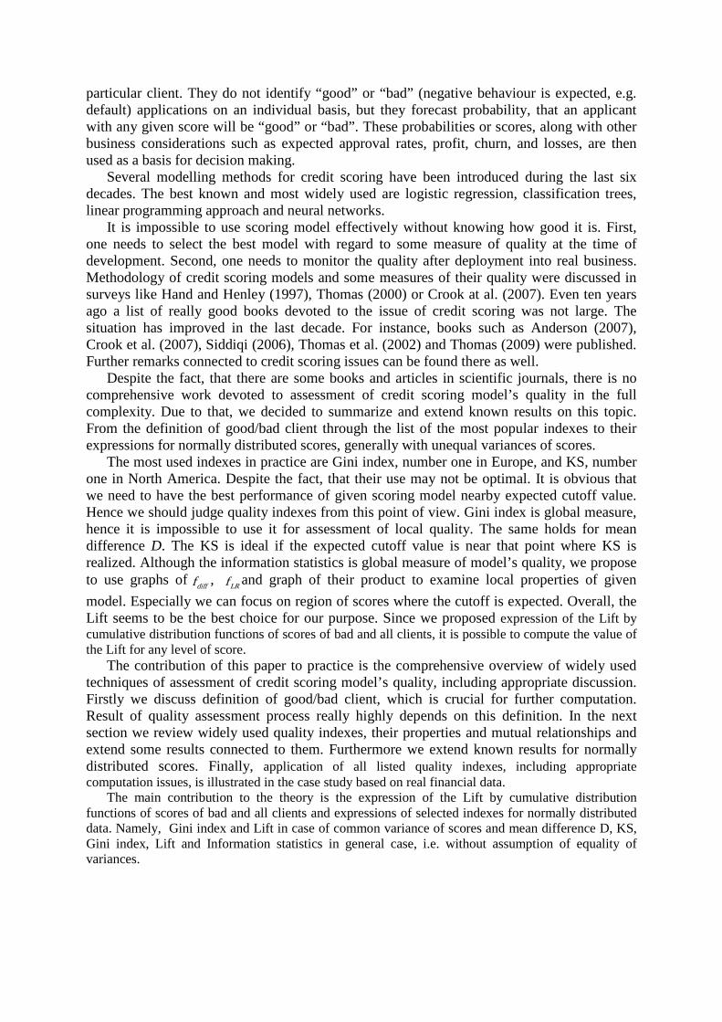
dependence of examined characteristics on gµ a 2gσ . In case of Figure 8 it was set 0=bµ ,

1=gµ and displayed value of Ival depending on the 2bσ , 2

gσ . Right-hand side of all these figures is contour graph of appropriate graph at left-hand side.

Figure 4: KS, 0=bµ , 12 =bσ

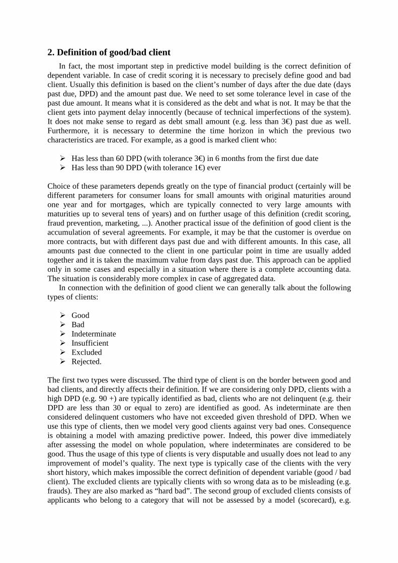
Figure 5: Gini coefficient, 0=bµ , 12 =bσ

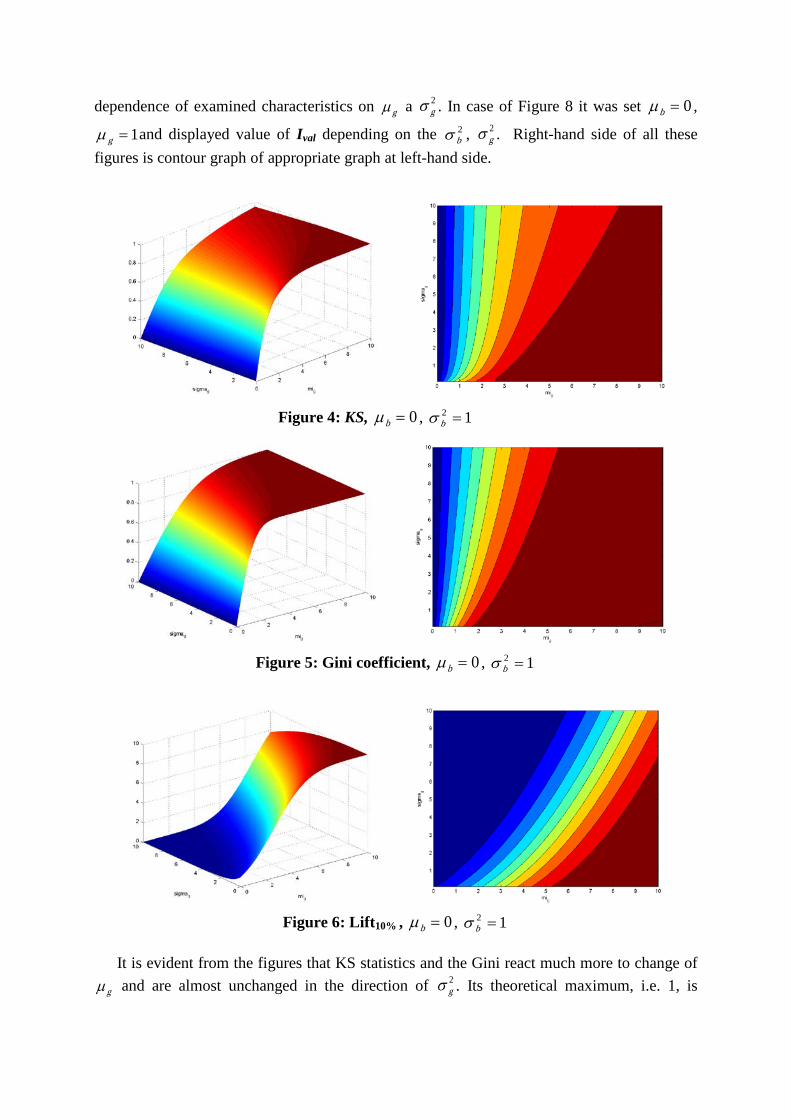
Figure 6: Lift10% , 0=bµ , 12 =bσ

It is evident from the figures that KS statistics and the Gini react much more to change of

gµ and are almost unchanged in the direction of 2gσ . Its theoretical maximum, i.e. 1, is

approximately reached in value 4=gµ , which is the value where relevant probability densities of good and bad clients almost do not overlap and hence the perfect separation of these two groups is reached. In case of Lift10%, see Figure 7, it is evident strong dependence on gµ . This time, however, the value of this index is significantly affected by 2

gσ .

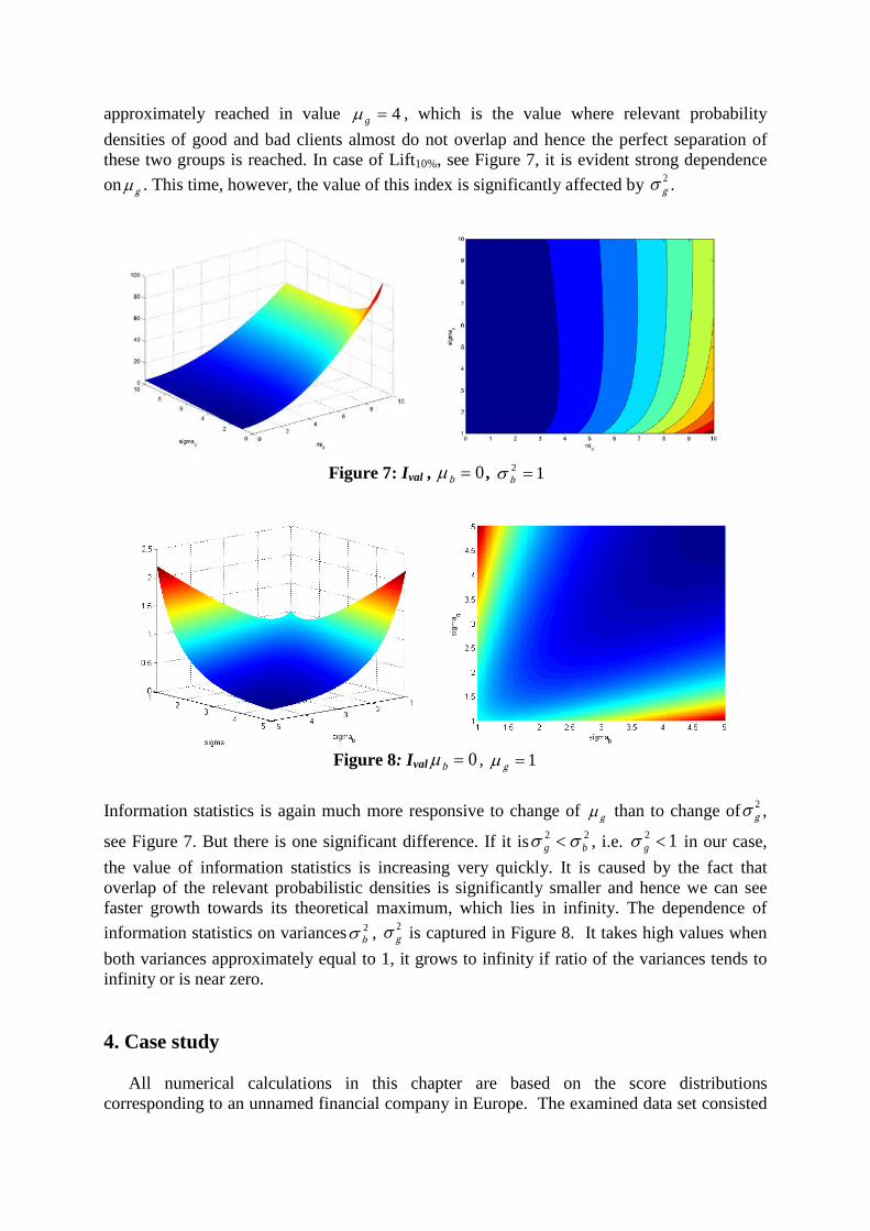
Figure 7: Ival , 0=bµ , 12 =bσ

Figure 8: Ival 0=bµ , 1=gµ

Information statistics is again much more responsive to change of gµ than to change of 2

gσ ,

see Figure 7. But there is one significant difference. If it is 22bg σσ < , i.e. 12 <gσ in our case,

the value of information statistics is increasing very quickly. It is caused by the fact that overlap of the relevant probabilistic densities is significantly smaller and hence we can see faster growth towards its theoretical maximum, which lies in infinity. The dependence of information statistics on variances 2

bσ , 2gσ is captured in Figure 8. It takes high values when

both variances approximately equal to 1, it grows to infinity if ratio of the variances tends to infinity or is near zero. 4. Case study

All numerical calculations in this chapter are based on the score distributions corresponding to an unnamed financial company in Europe. The examined data set consisted

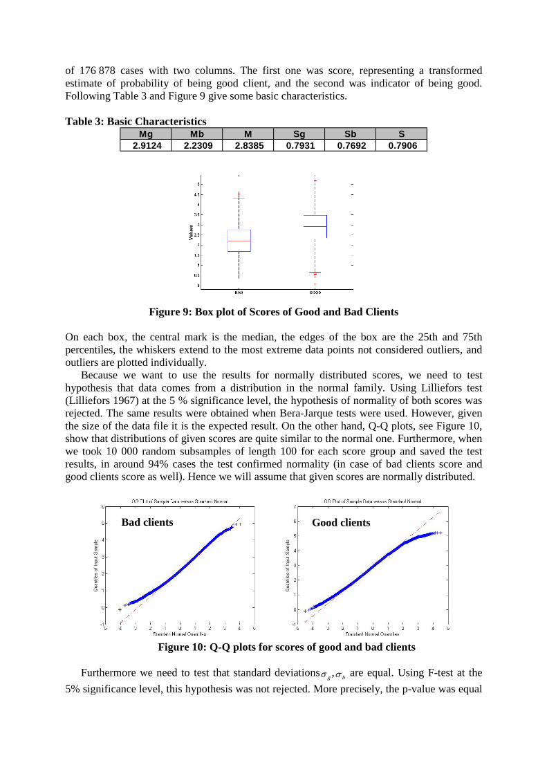
of 176 878 cases with two columns. The first one was score, representing a transformed estimate of probability of being good client, and the second was indicator of being good. Following Table 3 and Figure 9 give some basic characteristics. Table 3: Basic Characteristics

Mg Mb M Sg Sb S 2.9124 2.2309 2.8385 0.7931 0.7692 0.7906

Figure 9: Box plot of Scores of Good and Bad Clients

On each box, the central mark is the median, the edges of the box are the 25th and 75th percentiles, the whiskers extend to the most extreme data points not considered outliers, and outliers are plotted individually.

Because we want to use the results for normally distributed scores, we need to test hypothesis that data comes from a distribution in the normal family. Using Lilliefors test (Lilliefors 1967) at the 5 % significance level, the hypothesis of normality of both scores was rejected. The same results were obtained when Bera-Jarque tests were used. However, given the size of the data file it is the expected result. On the other hand, Q-Q plots, see Figure 10, show that distributions of given scores are quite similar to the normal one. Furthermore, when we took 10 000 random subsamples of length 100 for each score group and saved the test results, in around 94% cases the test confirmed normality (in case of bad clients score and good clients score as well). Hence we will assume that given scores are normally distributed.

Figure 10: Q-Q plots for scores of good and bad clients

Furthermore we need to test that standard deviations gσ , bσ are equal. Using F-test at the

5% significance level, this hypothesis was not rejected. More precisely, the p-value was equal

Bad clients Good clients

to 0.186, value of test statistics was equal to 1.063 and the 95% confidence interval for the true variance ratio was [0.912, 1.231].

The first insight into discriminatory power of the score we obtain using the graph of cumulative distribution functions of bad and good clients, see Figure 11. KS statistics, derived from this figure, was equal to 0.3394. The value of score, in which it was achieved, was equal to 2.556. Using result for normally distributed data we have, that KS was equal to 0.3335.

Figure 11: Cumulative Distribution Functions

The next Figure 12 shows Lorenz curve computed from our data set. It can be seen, that for example by rejection of 20% of good clients we reject 50% of bad clients at the same moment. The Gini index was equal to 0.4623 and c-statistics was equal to 0.7311.

Figure 12: Lorenz Curve

The last mentioned indicator of scoring model’s quality based on distribution function was

the Lift. The following Table 4 contains values of absolute and cumulative Lift corresponding to selected points on rejection scale. It is common to focus on the cumulative Lift value at 10% on this scale. In our case it was 2.80, which means that the given scoring model was 2.8 times better than random model at this level of rejection. Values in the last row of the table are computed by assumption of normality. The following Figure 13 shows Lift values on the whole rejection scale. Table 4: Absolute and Cumulative Lift

5% 10% 20% 30% 40% 50% 60% 70% 80% 90% 100%Abs. Lift 3,36 2,25 1,88 1,20 1,00 0,97 0,70 0,58 0,39 0,25 0,22Cum.Lift 3,36 2,80 2,34 1,96 1,72 1,57 1,43 1,31 1,19 1,09 1,00Cum.Lift_norm 3,67 2,95 2,30 1,95 1,72 1,54 1,40 1,28 1,18 1,09 1,00

% rejected (FALL)

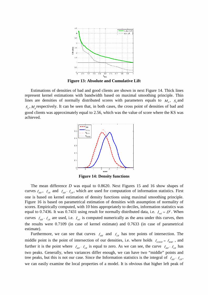
Figure 13: Absolute and Cumulative Lift

Estimations of densities of bad and good clients are shown in next Figure 14. Thick lines

represent kernel estimations with bandwidth based on maximal smoothing principle. Thin lines are densities of normally distributed scores with parameters equals to bM , bS and

gS , gM respectively. It can be seen that, in both cases, the cross point of densities of bad and good clients was approximately equal to 2.56, which was the value of score where the KS was achieved.

Figure 14: Density functions

The mean difference D was equal to 0.8620. Next Figures 15 and 16 show shapes of

curves difff , LRf and LRdiff ff ⋅ , which are used for computation of information statistics. First one is based on kernel estimation of density functions using maximal smoothing principle. Figure 16 is based on parametrical estimation of densities with assumption of normality of scores. Empirically computed, with 10 bins appropriately to deciles, information statistics was equal to 0.7436. It was 0.7431 using result for normally distributed data, i.e. 2DIval = . When curves LRdiff ff ⋅ are used, i.e. valI is computed numerically as the area under this curves, then the results were 0.7109 (in case of kernel estimate) and 0.7633 (in case of parametrical estimate).

Furthermore, we can see that curves difff and LRf has tree points of intersection. The middle point is the point of intersection of our densities, i.e. where holds BADGOOD ff = , and further it is the point where LRdiff ff ⋅ is equal to zero. As we can see, the curve LRdiff ff ⋅ has two peaks. Generally, when variances differ enough, we can have two “middle” points and tree peaks, but this is not our case. Since the Information statistics is the integral of LRdiff ff ⋅ , we can easily examine the local properties of a model. It is obvious that higher left peak of

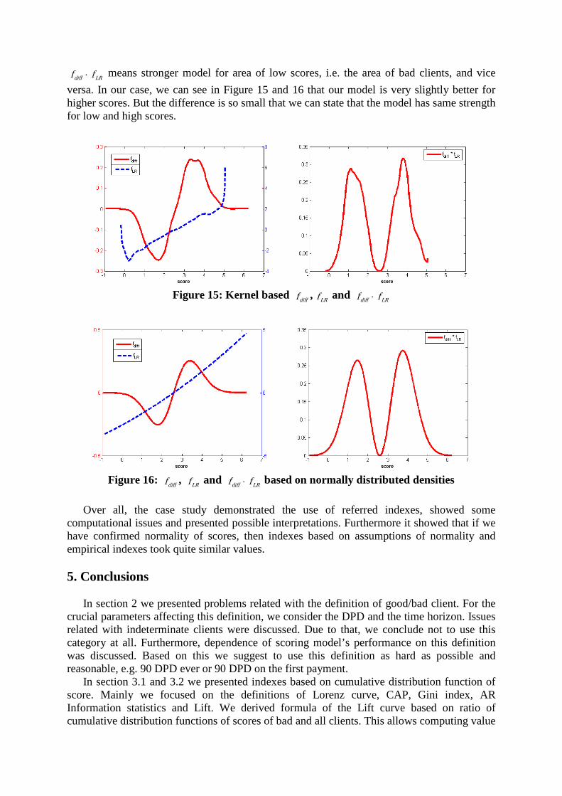
LRdiff ff ⋅ means stronger model for area of low scores, i.e. the area of bad clients, and vice versa. In our case, we can see in Figure 15 and 16 that our model is very slightly better for higher scores. But the difference is so small that we can state that the model has same strength for low and high scores.

Figure 15: Kernel based difff , LRf and LRdiff ff ⋅

Figure 16: difff , LRf and LRdiff ff ⋅ based on normally distributed densities

Over all, the case study demonstrated the use of referred indexes, showed some

computational issues and presented possible interpretations. Furthermore it showed that if we have confirmed normality of scores, then indexes based on assumptions of normality and empirical indexes took quite similar values.

5. Conclusions

In section 2 we presented problems related with the definition of good/bad client. For the crucial parameters affecting this definition, we consider the DPD and the time horizon. Issues related with indeterminate clients were discussed. Due to that, we conclude not to use this category at all. Furthermore, dependence of scoring model’s performance on this definition was discussed. Based on this we suggest to use this definition as hard as possible and reasonable, e.g. 90 DPD ever or 90 DPD on the first payment.

In section 3.1 and 3.2 we presented indexes based on cumulative distribution function of score. Mainly we focused on the definitions of Lorenz curve, CAP, Gini index, AR Information statistics and Lift. We derived formula of the Lift curve based on ratio of cumulative distribution functions of scores of bad and all clients. This allows computing value

of the Lift for any given score. On the other hand, it is much more useful to know the value of the Lift corresponding to some quantile of score. Due to that, we proposed the quantile form of the Lift. Despite high popularity of Gini index and KS, we conclude that Lift and figures of decomposed Information statistics are more appropriate for assessing local quality of a credit scoring model. Especially it is better to use them in case of asymmetric Lorenz curve. Using Gini index or KS during the development process could lead to selection of weaker model in this case.

Section 3.4 dealt with case of normally distributed scores. Firstly we assumed that standard deviations of scores of good and bad clients are equal. Known formulas for mean difference, KS and information statistics were appended by formulas for Gini index and Lift. Afterwards we did not assume the equality of standard deviations and derived expressions for all mentioned indexes in general. Behaviour of those indexes was illustrated in appropriate figures. We need to realize that all listed indexes are estimations of appropriate random statistics, whose exact values are unknown. Despite the fact that scores of credit scoring models usually are not exactly normally distributed, they are often very close to this distribution. In this case we suggest using expressions from this section, because we get more accurate estimates.

The application study in section 4 demonstrates on real financial data that all referred quantitative indexes and figures can be successfully used to measure the quality of credit scoring models. They can be used as benchmarks for comparison of several proposed models at the time of development. It should also be remembered that although the developed model can achieve excellent results, its actual quality is shown through time, i.e. after its deployment in practice. For this reason, it is therefore necessary to regularly monitor performance of the model. Once the performance of the model falls below given threshold, the model has to be redeveloped.

Although it may seem that everything about measurement of credit scoring model’s quality is solved, many questions for further research are still open. For instance, what is the effect of type of inputs into a model (continuous, categorized, WOE,…) and type of model (logistic regression, NN, Trees,…) on degree of asymmetry of Lorenz curve? What is the theoretical distribution of scores depending on type of inputs and type of model? What is the confidence band of the Lift curve? Last but not least open area for further research is a generalization of the expressions from section 3.4 for more general class of distributions such as generalized gamma or generalized beta distributions. Acknowledgments

We thank our colleagues for their valuable comments, and our departments for supporting

our research. References Anderson, R. (2007). The Credit Scoring Toolkit: Theory and Practice for Retail Credit Risk

Management and Decision Automation, Oxford: Oxford University Press. Berry, M.J.A. and Linoff, G.S. (2004). Data Mining Techniques: for Marketing, Sales, and

Customer Relationship Management, 2nd ed., Indianapolis: Wiley. Coppock, D.S. (2002). Why Lift?, DM Review Online, www.dmreview.com /news/5329-1.html. Accessed on 1 December 2009. Crook, J.N., Edelman, D.B., Thomas, L.C. (2007). Recent developments in consumer credit

risk assessment. European Journal of Operational Research, 183 (3), 1447-1465.

Engelmann B., Hayden, E. and Tasche, D. (2003), Measuring the Discriminatory Power of Rating System, http://www.bundesbank.de/download/bankenaufsicht/dkp/ 200301dkp_b.pdf. Accessed on 4 October 2010.

Giudici, P. (2003). Applied Data Mining: statistical methods for business and industry, Chichester : Wiley.

Hand, D.J. and Henley, W.E. (1997). Statistical Classification Methods in Consumer Credit Scoring: a review. Journal. of the Royal Statistical Society, Series A., 160,No.3, 523-541.

Harrell, F.E., Lee, K.L. and Mark, D.B. (1996). Multivariate prognostic models: issues in developing models, evaluating assumptions and adequacy, and measuring and reducing errors. Statistics in Medicine, 15, 361-387.

Koláček, J., Řezáč, M. (2010). Assessment of Scoring Models Using Information Value. In: Compstat’ 2010 proceedings. Paris.

Lilliefors, H.W. (1967). On the Komogorov-Smirnov test for normality with mean and variance unknown. Journal of the American Statistical Association, 62, 399-402.

Müller, M. and Rönz, B. (2000). Credit Scoring using Semiparametric Methods, In: Franke, J., Härdle, W. , Stahl, G. (Eds.). Measuring Risk in Complex Stochastic Systems, New York: Springer-Verlag.

Nelsen, R. B. (1998). Concordance and Gini’s measure of association. Journal of Nonparametric Statistics, 9, Isssue 3, 227–238.

Newson R. (2006). Confidence intervals for rank statistics: Somers' D and extensions. The Stata Journal, 6(3), 309-334.

Řezáč, M. (2003). Maximal Smoothing. Journal of Electrical Engineering, 54, 44-46. Siddiqi, N. (2006). Credit Risk Scorecards: developing and implementing intelligent credit

scoring, New Jersey: Wiley. Sobehart, J., S. Keenan, and R. Stein (2000), Benchmarking Quantitative Default Risk

Models: A Validation Methodology, Moody’s Investors Service. http://www.algorithmics.com/EN/media/pdfs/Algo-RA0301-ARQ-DefaultRiskModels.pdf. Accessed on 4 October 2010.

Somers R. H. (1962). A new asymmetric measure of association for ordinal variables. American Sociological Review, 27, 799-811.

Terrell, G.R. (1990): The Maximal Smoothing Principle in Density Estimation. Journal of the American Statistical Association, 85, 470-477.

Thomas, L.C. (2000). A survey of credit and behavioural scoring: forecasting financial risk of lending to consumers. International Journal of Forecasting, 16(2), 149-172 .

Thomas, L.C. (2009). Consumer Credit Models: Pricing, Profit, and Portfolio, Oxford: Oxford University Press.

Thomas, L.C., Edelman, D.B., Crook, J.N. (2002). Credit Scoring and Its Applications, Philadelphia: SIAM Monographs on Mathematical Modeling and Computation.

Wand, M.P. and Jones, M.C. (1995). Kernel Smoothing, London: Chapman and Hall. Wilkie, A.D. (2004). Measures for comparing scoring systems, In: Thomas, L.C., Edelman,

D.B., Crook, J.N. (Eds.), Readings in Credit Scoring. Oxford: Oxford University Press. Witzany, J. (2009). Definition of Default and Quality of Scoring Functions.

http://papers.ssrn.com/sol3/papers.cfm?abstract_id=1467718. Accessed on 1 September 2010.

Xu, K. (2003). How has the literature on Gini’s index evolved in past 80 years?, http://economics.dal.ca/RePEc/dal/wparch/howgini.pdf. Accessed on 1 December 2009.