accounting-based credit-scoring models: econometric investigations

Ph.D. Thesis

Accounting-based Credit-scoring models:

Econometric Investigations

Anne Dyrberg Rommer

Financial Markets, Danmarks Nationalbank, Copenhagen

and Centre for Applied Microeconometrics (CAM),

Institute of Economics, University of Copenhagen

June 2005

Preface

This Ph.D. thesis consists of a collection of articles. The articles have been written in the period 2002 – 2005

at Danmarks Nationalbank, which has provided me with a Ph.D. stipend, and at the University of

Copenhagen, where I have been enrolled in the Ph.D. program. Within the period, I spent five months at

University College London and half a year at the European Central Bank in Frankfurt.

I am grateful to Danmarks Nationalbank for providing me with a Ph.D. stipend, to my supervisor at the

University of Copenhagen, Hans Christian Kongsted, for being very actively involved in my work and for

providing many useful suggestions and new ideas, and to my manager at Danmarks Nationalbank, Jens

Lundager, for always being very supportive. Furthermore, I would like to thank my previous manager at the

World Bank, Amar Bhattacharya. It was my stay at the World Bank and the discussions with Amar, which

opened my eyes to the potential benefits of studying for a Ph.D.

I would also like to thank Danmarks Nationalbank and the University of Copenhagen for providing facilities in

two very different environments. I found it extremely stimulating to be a part of the research environment at

the University and the policy-oriented environment in the Bank. I also benefited from excellent visits to

University College London and the European Central Bank. I wish to thank colleagues at all four institutions

for making my time as a Ph.D. student enjoyable and for great discussions. A special thank to my co-authors

and to the great number of persons, who have commented on earlier versions of the four papers, which now

constitute my Ph.D.

Finally, I would like to thank family and friends, especially my husband Hans, for encouragement and

support.

Anne Dyrberg Rommer

Copenhagen, June 2005

Table of Contents Introduction and Summary

Chapter 1: “Firms in Financial Distress: An Exploratory Analysis” (page 1 – 82)

Chapter 2: “A Comparative Analysis of the Determinants of Financial Distress in French,

Italian and Spanish firms” (page 1 – 78)

Chapter 3: “Testing the Assumptions of Credit-scoring Models” (page 1 – 39)

Chapter 4: “Assessing the consequences of Basel II: Are there incentives for cherry-

picking when banks pool data across countries?" (joint with Lisbeth Borup and Dorte

Kurek) (page 1 – 32)

Introduction and Summary

This Ph.D. thesis consists of four chapters, which can be read independently. Chapters 1,

2 and 3 are independently authored and chapter 4 is co-authored. All chapters fall within

the field of accounting-based credit-scoring models. An accounting-based credit-scoring

model uses information extracted from company accounts, and perhaps also non-financial

information (such as age of the company). It estimates the probability that a particular firm

will default on its debt obligations. The four chapters are all examples of recent

contributions within the academic credit-scoring literature. Chapter 1 focus on a number of

analytical and modelling issues, and it sets up a credit-scoring model for Danish non-

financial firms. Chapter 2 investigates the determinants of corporate failure in Italian,

Spanish and French small and medium-sized companies. Chapter 3 discusses the

specification of credit-scoring models and provides a framework for the investigation of

various specification issues. Chapter 4 analyses the consequences on the calculated

capital requirements of setting up single-country versus multi-country credit-scoring

models. Some of the chapters have already proven useful for policy-making at Danmarks

Nationalbank as well as at the European Central Bank.

Assessing the degree of corporate sector credit risk facing banks is an important part of

the financial stability analysis conducted by central banks around the world, e.g. in

Australia, Austria, Belgium, Denmark, Finland, France, Norway, Spain, Sweden and UK.

Danmarks Nationalbank states in its first stand-alone publication on financial stability,

"Financial Stability 2002", that the "purpose of financial stability is to assess whether the

financial system is sufficiently robust so that problems in this sector will not impede the

functioning of the financial markets as efficient providers of capital for companies and

households". In Denmark, financial stability primarily depends on the soundness of the

banking institutions, which is heavily influenced by credit risk from exposures to Danish

companies. To assess the developments in the corporate sector, Danmarks Nationalbank

has set up a credit-scoring model as part of its financial stability monitoring system.

Currently, inspired by chapter 1 in this Ph.D. thesis, Danmarks Nationalbank uses the

methodology set up in the chapter to analyze firms in the non-financial sector, c.f.

"Financial Stability 2005".

A number of other central banks, which publish regular financial stability assessments,

have also set up credit-scoring models as part of their financial stability monitoring system,

e.g. Norges Bank and Banque de France. However, financial stability assessments are not

only at focus in national central banks. They are also at focus at international

organizations. An international organization such as the European Central Bank (ECB) has

not set up a credit-scoring model for the euro area non-financial corporate sector, but it

includes in its "Financial Stability Review – June 2005" a “special topic” on the

determinants of corporate failure in Italian, Spanish and French small and medium-sized

companies. The “special topic” gives a useful foundation for analyzing the degree of credit

risk facing banks, and thus it represents a key input for assessing risks and vulnerabilities

to financial stability. The analysis in ECB's "Financial Stability Review – June 2005" is

based on chapter 2 in this Ph.D. thesis.

Even though central banks have a natural interest in the safeguarding of financial stability,

it is only in recent years that numerous central banks have started publishing financial

stability reports. The rationale behind these reports, which Haldane (2005) calls “open

mouth” rather than “open market operations”, is that ex ante "detection of, and

transparency about, potential sources of financial instability can help engineer a pre-

emptive response by private market participants, which, in turn, might lower the probability

or impact of a crisis". As assessment of financial stability issues is a new policy area, there

are still many challenges and open issues: "… efforts should be focused on broadening

the available data, improving the empirical tools (methodologically and analytically), and

developing wide groups of indicators from which some predictive power can be derived

while also linking developments in these indicators to specific instruments", c.f. Houben,

Kakes and Schinasi (2004). Chapters 1 and 2 of this Ph.D. thesis should be seen as

attempts to fill out a small part of this wide agenda.

The Basel Committee’s "Revised Framework for Capital Measurement and Capital

Standards" (Basel II), which will enter into force in 2007, gives credit institutions the

possibility to use their internal models when calculating the minimum capital requirements.

The philosophy underlying the new rules is that the individual banks are best at assessing

their own "true" risk profile and the capital needed to support it. Basel II consists of 3

pillars. Pillar 1 is the minimum capital requirement to cover credit, market and operational

risk. Pillar 2 requires banks to assess their need for capital in relation to their overall risk

profile and supervisors to evaluate the banks' assessment of its capital need. Pillar 3 sets

out principles for banks' disclosure of information, to help facilitate market discipline.

Under pillar I, according to Basel II, the credit institutions have the choice of using either a

standard or one of two internal ratings-based approaches, when calculating their minimum

capital requirements. The standard approach is based on external credit ratings, e.g.

external rating agencies, whereas the internal rating-based (IRB) approaches are based

on the bank’s own estimates. In the foundation IRB approach, the bank estimates the

probability of default for its borrowers, while the supervisory authorities supply the other

risk factors, i.e. the loss given default, the maturity and the exposure at default. The

advanced IRB approach prescribes that banks themselves calculate all four risk

components. The capital requirement can be calculated by inserting the risk factors into

the formulas prepared by the Basel Committee.

It is necessary for credit institutions using the foundation or the advanced IRB approach to

estimate the probability that a borrower will default, e.g. using their internal credit-scoring

models. This new development implies that individual credit institutions, which traditionally

have used credit-scoring models to decide which clients to offer loans, and to detect

clients that are likely to default at an early stage, can now also use their internal credit-

scoring models for the calculation of their capital requirements. A bank's use of internal

models has to be approved by the supervisor. Hence, banking supervisors around the

world are considering credit-scoring models with renewed interest.

Chapter 4 in this Ph.D. thesis analyses the consequences on the calculated capital

requirements of setting up single-country versus multi-country credit-scoring models. The

results are of particular interest for banks operating in different countries, which plan to

pool data from their exposures in the various countries in order to estimate the probability

of default, and for banks planning to pool data with banks from other countries to make up

for an insufficient database. The paper shows how there may be incentives for banks to

choose the credit-scoring model, which delivers the lowest capital requirement without

considering what level of capital is actually appropriate to cover the overall credit risk, i.e.

to cherry-pick.

In addition to the strong interest in the topic of credit-scoring from the policy side and from

the practical side (from e.g. individual credit institutions), there is also a strong academic

interest in the topic, c.f. Balcaen and Ooghe (2004a) and Balcaen and Ooghe (2004b),

which surveys the literature on credit-scoring models. Some of the recent developments

are to model financial distress in a hazard model framework and to consider unobserved

heterogeneity. Chapter 3 in this Ph.D. thesis stresses the importance of the models being

well specified. In the chapter, various methodological aspects of credit-scoring models are

discussed and tested. Chapter 3 is an academic study, but it has practical implications, c.f.

chapter 4, which concludes that banks and regulators should have a careful look into the

sample selection and design of credit-scoring models, the statistical technique, the factors

that drive financial distress and the evaluation of the results. Chapter 3 sets a framework

for investigating various specification issues.

Two unique panel data sets have been constructed for this thesis. One was constructed

based on information on Danish firms from the Danish credit-rating agency KOB A/S, the

Danish Competition Authority (concentration index) and from a fellow Ph.D. student,

Kasper Nielsen (information on whether or not the firms are ultimate parent companies,

wholly-owned subsidiaries, owned by a fund or owned by the public sector). The other

data set was constructed based on information on French, Italian and Spanish firms. This

extensive dataset has been downloaded over three months from the pan-European

Amadeus database provided by Bureau van Dijk. As the data sets used for this thesis are

not documented elsewhere, detailed discussions of them are included in chapter 1 (Danish

data) and chapter 2 (French, Italian and Spanish data).

Below follows a summary of each of the chapters.

Chapter 1, which is called "Firms in Financial Distress: An Exploratory Analysis", focuses

on a number of analytical and modelling issues, and it sets up a credit-scoring model for

Danish non-financial firms. Compared to the existing literature, a number of novel

elements are introduced.

Firstly, the empirical distinction between three modes of exit is developed, namely

between firms in financial distress, voluntarily liquidated firms, and firms that have merged

with other firms or are acquired by other firms. As firms in the non-financial sector may go

out of business for these three reasons, the credit-scoring model is estimated as a

competing-risks model, and the probability of exiting to the various states is estimated

simultaneously as a multinomial logit model. Specification tests show that the right

specification of the model should include all three states and that all three states should be

treated as separate exits. To the best of my knowledge, it is the first study, which performs

these tests in this type of set-up where firms can exit for the three mentioned reasons.

Only one other credit-scoring study distinguishes between exit types. The industrial

organization studies, which do distinguish between exit types, distinguish between two

(and not three) modes of exit. Accordingly, this study extends previous studies on credit-

scoring, including the few studies which also use Danish companies.

Secondly, the data set used in the estimations is extraordinary, as it comprises the whole

population of Danish public limited liability companies (“aktieselskaber”) and private limited

liability companies (“anpartsselskaber”), mostly small and medium-sized enterprises,

covering all non-financial sectors of the Danish economy. The estimations cover around

30,000 firms and more than 150,000 firm-year observations, which existed between 1995

and 2001. This extraordinary data set enables me to use a much richer set of explanatory

variables than are usually included in such estimations. Furthermore the data set allows

me to use a definition of financial distress, which includes not only bankruptcies, but also

firms that have been compulsorily wound up, experienced a write down of their debt or a

forced sale.

Finally, the extensive data set allows a comparison of the results from the estimations

(parameter estimates and predictive performance) of the competing-risks model with the

results from an estimation of a hazard model, where firms that exit for other reasons than

financial distress are treated as censored or no longer observed. The comparison shows

that the results in the two set-ups are very alike. This is puzzling as one would think that

the competing-risks model would fare better. After all, the specification tests did show that

the right specification of the model should include all three states and that all three states

should be treated as separate exits. A way to interpret the results is that the correct

specification is the competing-risks specification, but that it seems as if the biases arising

from estimating a hazard model are relatively small, at least for the Danish corporate

sector.

"A Comparative Analysis of the Determinants of Financial Distress in French, Italian and

Spanish firms" is the title of chapter 2. The focus in this chapter is on the comparative

aspect. The determinants of corporate failure in French, Italian and Spanish firms are

investigated in order to find out whether the predictors of financial distress in the countries

are the same or not. There are few studies, which do compare the determinants of

financial distress across countries. To the best of my knowledge, this is the first

comparative accounting-based credit-rating study of a fairly homogenous group of

countries, and so it fills a gap in the literature.

The analysis uses a data set provided by Bureau van Dijk. The great virtue of the data set

is that it allows cross-country comparisons. On the negative side it should be mentioned

that the data set, when looking at each country individually, is not as good as some of the

data sets used in other individual country studies found in the literature (in the sense that a

number of firms drop out of the panel with no explanation).

In this chapter, credit-scoring models for France, Italy and Spain are set up. In order to

compare the determinants of financial distress, accounting-based credit-scoring models for

each country are estimated. The comparison of the significance and sign of the

determinants of financial distress in the three countries shows that although there are

some similarities across countries, there are also a lot of differences. Some of the

variables that behave similarly across countries are the earnings ratio and the solvency

ratio. The variables, whose effect differs between the countries in terms of whether or not

they are significant or what sign they have, are the loans to total assets ratio, size, age,

legal form and a variable, which measures the concentration of ownership.

In addition to the individual credit-scoring models, a model including all countries is

estimated. The significance and sign of the parameter estimates and the predictive abilities

of the individual country credit-scoring models and the common model are compared. The

comparison shows that the common model delivers results that differ to quite an extent

from the individual country credit-scoring models.

The analysis has implications for at least two policy areas: financial stability analysis and

Basel II. An important part of financial stability analysis entails assessing the degree of

corporate sector credit-risk facing banks. For financial stability analysis on a euro area

wide basis, it is important to ascertain whether common or country-specific factors drive

corporate failures. If factors that give rise to financial distress are the same across

countries, then aggregation of individual corporate sectors into a single group is justified,

whereas, if country specific factors are important, this would call for analyzing conditions in

each individual corporate sector. Basel II allows that the credit institutions estimate their

minimal capital requirements using their internal models. As valid estimates of the

probability of default for individual banks require a considerable amount of data, Basel II

allows for banks to pool their data with other banks in order to overcome their data

shortcomings. Therefore a number of international data pooling projects have emerged

where banks from various countries pool their data. Because of this development and as

many credit institutions in Europe have cross-border activities, the choice between setting-

up individual country credit-scoring models or a common credit-scoring model is relevant

for banks' calculation of capital requirements.

The analysis shows that the factors that drive financial distress in the three analyzed

countries are not the same. Hence, the implication for the relevant policy areas – financial

stability and Basel II – is that the countries should be analyzed and assessed on an

individual basis.

Chapter 3, "Testing the Assumptions of Credit-scoring Models", discusses a number of

issues that are relevant when setting up a credit-scoring model and tests the assumptions

used in accounting-based credit-scoring models. Specification issues are important to

consider, as more powerful models are more profitable than weaker ones, c.f. Stein

(2005). Most methodological papers compare logit analysis to other estimation methods

such as discriminant analysis and various non-parametric techniques. Using an extensive

data set on Danish non-financial sector firms, the chapter makes a non-standard

comparison of two hazard models with differently specified hazard functions: one with a

logit specification and the other with a probit specification. The specification of the credit-

scoring model as a hazard model allows me to include information leading up to “financial

distress”. The logistic distribution is similar to the normal, except in the tails, and so the

logit and the probit model tend to give similar probabilities, except in the tails. The tails of

the logistic distribution are considerably heavier than the tails of the normal distribution, i.e.

in the tails of the logistic distribution, the probabilities are larger compared to the normal

distribution. The comparison of the two distributions is relevant, as the sample contains

very few responses, and thus, the properties at the tails of the distributions are at focus.

The logit and the probit specification are formally tested against each other, using two

tests which are probably used for the first time within the credit-scoring literature.

The estimations assume that if two firms have identical values of the covariates, they also

have identical hazard functions, that is, all differences between firms are assumed to be

captured using observed explanatory variables, or, in other words, unobserved

heterogeneity is assumed away. The presence of unobserved heterogeneity can cause

several problems, therefore, as a specification check, the probit and the logit specification

for the hazard function are extended to include unobserved heterogeneity.

In addition to investigating the various specifications of the hazard function, the chapter

discusses the treatment in the literature of different types of exits. There are recent

examples of studies within the credit-scoring and the industrial organization literature,

which still do not distinguish between exit types. As the extensive data set allows

comparisons of different specifications, the chapter explores the consequences of setting

up 1) a hazard model where the event “financial distress” is modelled and where firms that

exit for other reasons than financial distress are treated as censored or no longer observed

and 2) a hazard model where the general exit event is modelled (i.e. not split up on exit

type). To the best of my knowledge, no other paper provides the estimations of a hazard

model where firms in financial distress are modelled and where the other forms of exits are

treated as censored, versus a model which pools the three modes of exit (financial

distress, voluntary liquidation and mergers and acquisitions etc.).

The conclusions in the chapter are the following: Firstly, there seems to be no major

differences between the logit and the probit specification. Despite the fact that our formal

tests gave conflicting results, the full analysis (which includes the tests, the estimated

parameter estimates and the predictive abilities of the models) confirms that it is difficult to

distinguish between the logit and the probit model, even at the tails of the distributions.

Secondly, unobserved heterogeneity seems to be unimportant, probably because a

number of proxies are used for inherently unobservable variables. Thirdly, the results differ

depending on the modelled event (financial distress versus pooled exits). This is the case

for the estimated parameters as well as the predictive abilities of the models, no matter

whether the specification for the hazard functions is the logit or the probit specification.

This result highlights that it is important to think carefully about the specification of the

model in order not to mix “apples and pears”.

The practical implication of the chapter is that it is important to think about the specification

of credit-scoring models. A number of issues are highlighted and investigated in the

chapter using an extensive data set on Danish non-financial sector firms. It is crucial to

understand that the results depend on the portfolio under consideration, and hence, that

every model builder has to think carefully about the issues. The chapter provides a

framework for such investigations.

The last chapter, chapter 4, is called “Assessing the consequences of Basel II: Are there

incentives for cherry-picking when pooling data across countries?". This chapter presents

the Basel II rules and shows how banks might have incentives to choose the credit-scoring

model, which delivers the lowest capital requirement. The chapter sets up policy

recommendations for banking supervisors.

Basel II facilitates the use of banks' internal models to estimate probability of default when

calculating the minimum capital requirement using the internal ratings-based approaches.

Valid estimates of the probabilities of defaults require a considerable amount of data and

default observations. Basel II allows for banks to pool their data to overcome their data

shortcomings and a number of international data pooling projects have emerged. This

highlights that even international banks may need more data to fulfil the requirements of

Basel II.

To the best of my knowledge, no study to date has compared the banks' capital

requirements calculated on the basis of probabilities of defaults estimated from single-

country credit-scoring models and multi-country credit-scoring models, and accordingly no

study has discussed the incentive structure this might create for banks pooling data.

The purpose of this chapter is to illustrate the consequences on the calculated capital

requirements of pooling data for estimation of probability of default from several countries.

A hypothetical portfolio of loans to small and medium-sized enterprises for a hypothetical

bank operating in France, Italy and Spain is constructed. The portfolio is based on real

world data extracted from the Amadeus database. The probabilities of defaults are

estimated on the basis of single-country credit-scoring models and on the basis of multi-

country credit-scoring models with pooled data from the three countries. The estimated

probabilities of defaults are then used to calculate the minimum capital requirements.

The result shows that there might be incentives for cherry-picking, i.e. that banks are

motivated for choosing a certain method because it results in a lower capital requirement.

The calculated capital requirements vary with up to 18 per cent depending on the choice of

method for the hypothetical bank. Calculated for the individual countries, it varies up to 47

per cent. The results are of particular interest for banks operating in several countries,

which plan to pool data from the various countries in order to estimate probabilities of

defaults, maybe due to lack of a sufficient single-country database. They are equally

interesting for banks planning to pool data with banks from other countries to make up for

an insufficient database.

Though my default definition is the same for the three countries and I have controlled for

variables such as age, size, legal form and sector of each firm, quite large differences in

terms of the resulting minimum capital requirements for the portfolio in each of the three

countries are found, when the probabilities of defaults are estimated using a single-country

credit-scoring model compared to using multi-country credit-scoring models. I find that it is

not sufficient for banks to apply similar definitions of default and similar accounting

regimes in the countries. Banks and regulators should also have a thorough look into the

models, especially the factors that drive financial distress.

Literature Balcaen S. and H. Ooghe, 2004a. 35 years of studies on business failure: an overview of the classical statistical methodologies and their related problems. Working Paper 2004/248, Faculteit Economie en Bedrijfskunde Balcaen, S. and H. Ooghe, 2004b. Alternative methodologies in studies on business failure: do they produce better results than the statistical methods? Working Paper 2004/249, Faculteit Economie en Bedrijfskunde Basel Committee on Banking Supervision, 2004. International Convergence of Capital Measurement and Capital Standards. A Revised Framework. Bank for International Settlements, June 2004. Danmarks Nationalbank, 2002. Financial Stability 2002. Copenhagen, Denmark: Danmarks Nationalbank Danmarks Nationalbank, 2005. Financial Stability 2005. Copenhagen, Denmark: Danmarks Nationalbank European Central Bank, 2005. Financial Stability Review – June 2005. European Central Bank Haldane, A., 2005. A framework for financial stability. Central Banking, vol. XV, no. 3 Houben, A., Kakes, J. and G. Schinasi, 2004. Toward a Framework for Safeguarding Financial Stability. WP/04/101, IMF Working Paper, International Monetary Fund Stein, R., 2005. The relationship between default prediction and lending profits: Integrating ROC analysis and loan pricing. Journal of Banking & Finance, vol. 29, pp. 1213-1236

"Those who have knowledge don't predict.

Those who predict don't have knowledge."

Lao Tzu

CHAPTER 1

Anne Dyrberg Rommer*

Firms in Financial Distress: An Exploratory Analysis

* This chapter is based on A. Dyrberg, 2004, Firms in Financial Distress: An Exploratory Analysis, Working Paper no. 17, Danmarks Nationalbank. The author would like to thank Hans Christian Kongsted, Steen Winther Blindum, Mette Ejrnæs, David Lando, Helene Bie Lilleør, Jesper Rangvid and colleagues at the Danish Central Bank for commenting on this or earlier versions of the paper and seminar participants at the Danish Graduate Program in Economics workshop held 13. - 14. November 2003, Centre for Applied Microeconometrics (University of Copenhagen) seminar held 18. November 2003, Danish Central Bank seminar held 27. November 2003, C.R.E.D.I.T. 2004 conference on “Validation of Credit Risk Models” held in Venice 30. September - 1. October and Bundesbank seminar held 6. December 2004. Corresponding address is Anne Dyrberg Rommer, Financial Markets, Danmarks Nationalbank, Havnegade 5, DK-1093 Copenhagen, Denmark. Phone: + 45 33 63 63 63. Email: [email protected]

ABSTRACT:

The aim of this paper is to present the set-up of an accounting-based credit-scoring model and to estimate such a model using Danish data. The paper focuses on a number of analytical and modelling issues. The empirical distinction between three modes of exit is developed, namely between firms in financial distress, voluntarily liquidated firms, and firms that have merged with other firms or are acquired by other firms. As firms in the non-financial sector may go out of business for these three reasons, the credit-scoring model is estimated as a competing-risks model, and the probability of exiting to the various states is estimated simultaneously as a multinomial logit model. Specification tests show that the right specification of the model should include all three states and that all three states should be treated as separate exits. We compare the results from the estimations of the competing-risks model with the results from an estimation of a hazard model, where firms that exit for other reasons than financial distress are treated as censored or no longer observed.

Chapter 1 - Firms in Financial Distress: An Exploratory Analysis

1. Introduction and Literature Review ...................................................................5

2. Economic Theory and its implication for the Explanatory Variables...............11 2.1. The Core Variables.........................................................................13 2.1.1. Duration Dependence.....................................................................13 2.1.2. Firm Performance...........................................................................16 2.1.3. Firm Size.........................................................................................16 2.2. Proxies............................................................................................19 2.2.1. Diversification .................................................................................19 2.2.2. The Location of the Firm.................................................................21 2.2.3. Concentration .................................................................................21 2.2.4. Public/fund Ownership....................................................................22 2.2.5. Critical Comments from the Auditors..............................................22 2.2.6. Wholly Owned Subsidiaries and Ultimate Parent Companies .......23 2.2.7. Limited Liability ...............................................................................24 2.2.8. Companies Listed on a Stock Exchange........................................25 2.3. Controls ..........................................................................................25 2.3.1. Sector Affiliation..............................................................................25 2.3.2. Macroeconomic Effects ..................................................................26 2.3.3. Firms with a Primary Bank..............................................................27

3. Data and the Construction of the Dependent Variable ...................................27 3.1. The Data Base and Sample Selection ...........................................27 3.2. The Construction of the Dependent Variable .................................30

4. Econometric Theory........................................................................................34 4.1. Competing-risks model...................................................................35 4.2. Independence of Irrelevant Alternatives.........................................39 4.3. Pooling States in the Multinomial Logit Model................................40

5. Results ............................................................................................................41 5.1. Specification Tests..........................................................................42 5.2. Parameter Estimates ......................................................................44 5.3. Goodness-of-fit and Robustness....................................................49 5.4. Proportion of Correct Predictions ...................................................51

6. A Comparison with a Simple Financial Distress Model ..................................55 6.1. Interpretational Differences in the Competing-risks Model and

the Simple Financial Distress Model ..............................................56 6.2. Parameter Estimates and the Proportion of Correct Predictions ...60

7. Conclusion ......................................................................................................62

8. LITERATURE..................................................................................................66


9. Appendix: Data................................................................................................71

10. Appendix: Figures and Tables ........................................................................79

11. Appendix: Predictions .....................................................................................82


5

1. Introduction and Literature Review The aim of this paper is to present the set-up of an accounting-based credit-scoring model and to estimate such a model using Danish data. The paper focuses on a number of analytical and modelling issues.

Models that can predict the firms that end up in financial distress are used by central banks and financial institutions.

In central banks their predictions serve as input to financial stability assessments. Danmarks Nationalbank is one among many central banks, which have started publishing financial stability assessments on a regular basis, see e.g. Danmarks Nationalbank (2005). The purpose of the analysis is to identify the risks currently faced by the financial sector. The stability of the financial sector depends on the financial situation of its customers and so analysis with special emphasis on the banks and of how the financial sector is affected by the finances of companies and households are crucial. As the majority of lending from Danish banks is granted to companies in Denmark, it is primarily the developments in the Danish corporate sector that affect the banks. Accordingly a model that can predict the firms that end up in financial distress is of particular interest. Currently, Danmarks Nationalbank use the methodology set up in this paper to analyze firms in the non-financial sector, c.f. Danmarks Nationalbank (2005). Examples of other central banks, which have set up credit-scoring models, are Banque de France (Bardos (1998) and Bardos (2001)), Norges Bank (Bernhardsen (2001)) and Bank of England (Bunn and Redwood (2003) and Bunn (2003)). The European Central Bank has set up credit-scoring models and analyzed the determinants of financial distress in French, Italian and Spanish firms, c.f. European Central Bank (2005), which is based on Rommer (2005a).

Individual financial institutions use credit-scoring models to assess the quality of a particular borrower. The topic of credit scoring has received renewed interest as Basel II opens up for the possibility that the credit institutions themselves can calculate the minimal capital requirements using their own internal models. According to Basel II the credit institutions have a choice of using a standard approach or one of two internal ratings-based approaches.1 Using either of the two internal ratings-based approaches, the credit institutions themselves must assess the probability that a borrower will default during the following year. The model framework developed in this paper can be used in credit institutions to assess the probability that a borrower may default. The academic literature on Basel II issues is expanding rapidly at the moment. Recent contributions are Borup, Kurek and Rommer (2005), Henneke and Trück (2005) and Elizalde and Repullo (2004).

1 For further details, see Basel Committee on Banking Supervision (2004).


6

The literature on bankruptcy prediction is not new. The study of Beaver from 1966 is considered the pioneering work on bankruptcy-prediction models. By now, there exist a number of studies, which discusses the developments in the literature. Examples of surveys are Jones (1987), Dimitras, Zanakis and Zopounidis (1996), Altman and Saunders (1998) and Balcaen and Ooghe (2004). Some of the often-quoted parametric credit-rating studies are Beaver (1966), Altman (1968), Ohlson (1980) and Shumway (2001).

As mentioned, Beaver (1966) is considered the pioneering work on bankruptcy-prediction models. The “theory” behind the model can best be explained within the framework of a “cash-flow”. Beaver (1966:80) writes: “The firm is viewed as a reservoir of liquid assets, which is supplied by inflows and drained by outflows. The reservoir serves as a cushion or buffer against variations in the flows. The solvency of the firm can be defined in terms of the probability that the reservoir will be exhausted at which point the firm will be unable to pay its obligations as they mature (i.e., failure)”. Using univariate discriminant analysis he shows that financial ratios can be used to predict corporate failure. Since the study of Beaver (1966), bankruptcy studies have been improved and refined. Altman (1968) introduces multivariate discriminant analysis. Later the centre of research shifts to logit/probit models, see e.g. Ohlson (1980), who advocates for the use of the logit model. Shumway (2001:101) criticises the approaches taken in these older studies, as they are single-period classification models: "By ignoring the fact that firms change through time, static models produce bankruptcy probabilities that are biased and inconsistent estimates of the probabilities that they approximate." Instead he proposes to use a hazard model.

The focus in this paper is on parametric estimation. As firms in the non-financial sector may go out of business for various reasons (financial distress, voluntary liquidation, and because they are merged or acquired, etc.) the estimation of a parametric competing-risks model seems appropriate. The estimation strategy of Allison (1982) is followed and the probability of exiting to the various states is estimated simultaneously as a multinomial logit model. The specification of the credit-scoring model as a competing-risks model enables the user of the model, not only to use the model for financial distress prediction, but also to analyze the differences between the factors that drive financial distress, voluntary liquidations, and mergers and acquisitions. Furthermore, the model can be used to assess the effect on a possible increase or decrease in one or more explanatory variables (i.e. as a stress-testing tool). This is possible as the specification of the model as a multinomial logit model allows that if a variable x has a positive coefficient, an increase in the variable may lead to an increase in the probability of exiting as a financially distressed firm, but it need not be the case, as the probability of another outcome may increase by even more (e.g. the probability of exiting to voluntary liquidation). This is not the case in the hazard model set up in Shumway (2001),


7

where firms that exit for other reasons than financial distress are treated as censored or no longer observed. If a variable x has a positive coefficient in this set up one knows that every increase in x results in an increase in the probability of the designated outcome.

As the competing-risks model is estimated as a multinomial logit model, two specification tests for multinomial logit models are presented and performed. The first is the test for the independence of irrelevant alternatives (IIA assumption). The second is a test for pooling states in the multinomial logit model. The specification tests show, that the competing-risks model should be specified as a multinomial logit model in which all states are included (according to the IIA test neither voluntary liquidations or mergers and acquisitions, etc., should be left out of the multinomial logit model) and where voluntary liquidations and mergers and acquisitions, etc., are treated as separate exits (and not lumped together with active firms. This is the result from the test for the pooling of states). The results from the estimations (parameter estimates and predictive ability) are compared to the results from an estimation of a hazard model where firms that exit for other reasons than financial distress are treated as censored or no longer observed. This corresponds to the set up in Shumway (2001), c.f. above and below.

The analysis here is in line with Schary (1991), who advocates for a richer discussion of the determinants of exits. She distinguishes between bankruptcy, voluntary liquidation and mergers and acquisitions. Unfortunately, her sample is rather limited2, which makes it difficult to draw conclusions. The analysis in Schary (1991) is the only credit-rating study we could find, which models firms in financial distress, voluntary liquidations and mergers and acquisitions. Most credit-scoring studies do not distinguish between these exit types. Beaver (1966), Altman (1968) and Ohlson (1980) do not mention firms that exit for other reasons than financial distress, and Shumway (2001) only mentions as an aside, that firms are treated as censored or no longer observed, when they leave the sample for other reasons than financial distress. This last point is highlighted in Balcaen and Ooghe (2004) who write, that hazard models consider firms that exit for other reasons than financial distress to be censored. Lando (2004:81), who discusses statistical techniques for analyzing defaults, writes that in the hazard model we need to think “of this censoring mechanism as being unrelated to the default event. … In the real world, we see nondefaulted firms as part of mergers or target of takeover, and although in some sectors such activity may be related to an increased default probability, it does not seem to be a big problem in empirical work.”

In the industrial organization literature there has been some attempts to study the factors leading firms to exit, split up on type of exit. Papers that are

2 In her empirical analysis of the declining cotton industry between 1924 and 1940 in New England she

analyzes a sample of 61 firms.


8

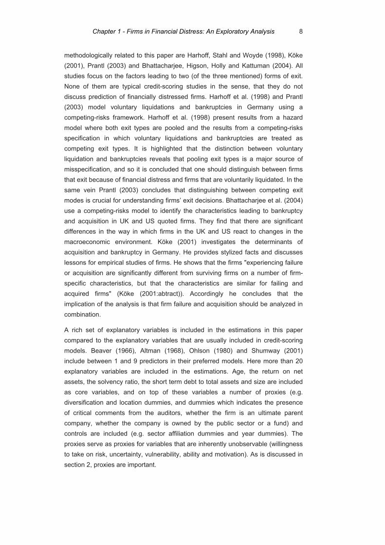
methodologically related to this paper are Harhoff, Stahl and Woyde (1998), Köke (2001), Prantl (2003) and Bhattacharjee, Higson, Holly and Kattuman (2004). All studies focus on the factors leading to two (of the three mentioned) forms of exit. None of them are typical credit-scoring studies in the sense, that they do not discuss prediction of financially distressed firms. Harhoff et al. (1998) and Prantl (2003) model voluntary liquidations and bankruptcies in Germany using a competing-risks framework. Harhoff et al. (1998) present results from a hazard model where both exit types are pooled and the results from a competing-risks specification in which voluntary liquidations and bankruptcies are treated as competing exit types. It is highlighted that the distinction between voluntary liquidation and bankruptcies reveals that pooling exit types is a major source of misspecification, and so it is concluded that one should distinguish between firms that exit because of financial distress and firms that are voluntarily liquidated. In the same vein Prantl (2003) concludes that distinguishing between competing exit modes is crucial for understanding firms’ exit decisions. Bhattacharjee et al. (2004) use a competing-risks model to identify the characteristics leading to bankruptcy and acquisition in UK and US quoted firms. They find that there are significant differences in the way in which firms in the UK and US react to changes in the macroeconomic environment. Köke (2001) investigates the determinants of acquisition and bankruptcy in Germany. He provides stylized facts and discusses lessons for empirical studies of firms. He shows that the firms "experiencing failure or acquisition are significantly different from surviving firms on a number of firm-specific characteristics, but that the characteristics are similar for failing and acquired firms" (Köke (2001:abtract)). Accordingly he concludes that the implication of the analysis is that firm failure and acquisition should be analyzed in combination.

A rich set of explanatory variables is included in the estimations in this paper compared to the explanatory variables that are usually included in credit-scoring models. Beaver (1966), Altman (1968), Ohlson (1980) and Shumway (2001) include between 1 and 9 predictors in their preferred models. Here more than 20 explanatory variables are included in the estimations. Age, the return on net assets, the solvency ratio, the short term debt to total assets and size are included as core variables, and on top of these variables a number of proxies (e.g. diversification and location dummies, and dummies which indicates the presence of critical comments from the auditors, whether the firm is an ultimate parent company, whether the company is owned by the public sector or a fund) and controls are included (e.g. sector affiliation dummies and year dummies). The proxies serve as proxies for variables that are inherently unobservable (willingness to take on risk, uncertainty, vulnerability, ability and motivation). As is discussed in section 2, proxies are important.


9

Compared to Beaver (1966), Altman (1968), Ohlson (1980) and Shumway (2001), the data used for this study is unique as it comprises information on the whole population of Danish public and private limited liability companies, mostly small and medium-sized enterprises, covering all non-financial sectors of the Danish economy. The database consists of altogether more than 30,000 firms and more than 150,000 firm-year observations, and it includes 2,617 firms in financial distress, 907 voluntarily liquidated firms, and 1,233 firms that are acquired/have merged with other firms, etc. In contrast, Beaver (1966) is based on 79 non-failed and 79 failed firms (listed industrials), Altman (1968) is based on 33 non-bankrupt and 33 bankrupt firms (listed manufacturing companies), Ohlson (1980) is based on 2,058 non-bankrupt and 105 bankrupt firms (industrials with traded equity) and Shumway (2001) is based on 28,664 firm-year observations and 239 bankruptcies (industrials with traded equity).

Few credit-scoring studies use as much information as we have.3 Two studies, which use more information than we do in terms of number of firm-years and bankruptcies, are Bernhardsen (2001) and Lykke, Pedersen and Vinther (2004)4. Bernhardsen (2001), who sets up a model of the Norwegian non-financial sector, includes around 400,000 firm-year observations and 8,500 bankruptcies. His model covers the period 1988-1999. Lykke, Pedersen and Vinther (2004) set up a model of the Danish non-financial sector for the period 1995-1999. Their model contains approximately 300,000 annual accounts of which almost 8,000 are from failed companies.5 Both studies model the exit to financial distress and do not distinguish between exit types. They also include fewer explanatory variables than this study does.

This study not only considers the whole population of Danish firms and therefore uses a data set with many more observations than is commonly used in credit-scoring studies, it furthermore improves the analysis of financially distressed firms by defining firms in financial distress as bankrupt companies, firms that have been compulsorily wound up (“tvangsopløst”), experienced a write down of their debt (“tvangsakkord”) or a forced sale (“tvangsauktion”). Accordingly, this paper

3 The sample is also impressive compared to the samples used in the industrial organization studies,

which are mentioned. Harhoff et al. (1998) use a sample of about 11,000 West German firms between 1990 and 1994. The sample in Prantl (2003) includes around 14,000 East and West German firms with a firm formation date between 1990 and 1993. The sample in Bhattacharjee et al. (2004) consists of about 13,700 US industrial firms over the period 1969 to 2000, and 4,300 UK listed industrials over the period 1965 to 1998. Köke uses a sample of about 1,700 German firms for the years 1986-1995.

4 Lykke, Pedersen and Vinther (2004) is based on Pedersen (2002). 5 Lykke, Pedersen and Vinther (2004) use data from the Danish credit rating agency KOB A/S. Data

used in this paper is also from the Danish credit rating agency KOB A/S. The reason why Lykke, Pedersen and Vinther (2004) include more financial statements in their analyses compared to this study is, that they choose to include companies with total assets more than kr. 50,000. In this study it is chosen to include companies with at least 5 employees and total assets of at least kr. 500,000 (the year they are included in the data set).


10

accommodates the critique of other models, which is posed e.g. by Lau (1987) and Jones and Hensher (2004). Lau (1987) and Jones and Hensher (2004) criticize credit-scoring studies for being too simple, as they only model failure as a simplistic binary classification of failure or non-failure. The approach is called into question, as the strict legal concept of bankruptcy may not always reflect the true underlying economic reality of corporate financial distress. Lau (1987) estimates a financial distress model as a multinomial logit model in which five states are included (financial stability (350 firms), omitting or reducing dividend payments (20 firms), technical default and default on loan payments (15 firms), protection under chapter X or XI of the Bankruptcy Act (10 firms) and bankruptcy or liquidation (4 firms)). Inspired by Lau (1987), Jones and Hensher (2004) propose to estimate a financial distress model as an ordered mixed logit model in which three states are included (non-failed firms (2,838 firms), insolvent firms (e.g. loan default) (78 firms) and firms who filed for bankruptcy followed by the appointment of liquidators, insolvency administrators, or receivers (116 firms)). In this study firms in financial distress, defined as is explained above, are analyzed as one group as a whole. The number of firms in financial distress used in this study is 2,617, i.e. it is much larger the numbers of firms in financial distress used in both Lau (1987) and Jones and Hensher (2004). Further work within the area could be to analyze separately the events which here in this paper constitute the group financially distress firms.

Furthermore, this analysis extends the previous credit-scoring studies using Danish companies. Compared to Røjkjær and Klinker (1994), which use discriminant analysis to analyse 58 large Danish firms, this study extends the analysis by using an advanced econometric method, a larger number of explanatory variables and a much larger dataset. Compared to Lykke, Pedersen and Vinther (2004), which use logistic regression to analyse approximately 300,000 annual accounts, this study extends the analysis by distinguishing between three exit modes and by including a much larger number of explanatory variables. Furthermore, the estimation period is extended. The model presented in Lykke, Pedersen and Vinther (2004) is estimated using data from 1995-1999. In this paper the model is estimated using data from 1995-2001. A larger number of explanatory variables are used in this paper compared to Lykke, Pedersen and Vinther (2004). E.g. the data set used in this paper is augmented to include a concentration index and information on ownership. Compared to Lykke, Pedersen and Vinther (2004) this paper also includes a richer discussion of the data set from the Danish credit-rating agency KOB A/S.

In sum, compared to the existing literature this study takes the analysis a step further. A number of novel elements to the empirical analysis are introduced.

Firstly, the empirical distinction between three modes of exit is developed, namely between firms in financial distress, voluntarily liquidated firms, and firms that have merged with other firms or are acquired by other firms, etc. As firms in the non-


11

financial sector may go out of business for these three reasons, the credit-scoring model is estimated as a competing-risks model, and the probability of exiting to the various states is estimated simultaneously as a multinomial logit model. Specification tests show that the right specification of the model should include all three states and that all three states should be treated as separate exits. To the best of our knowledge, it is the first study, which performs these tests in this type of set-up where firms can exit for the three mentioned reasons. Only one other credit-scoring study distinguishes between exit types, and the industrial organization studies, which do distinguish between exit types, distinguish between two (and not three) modes of exit. Accordingly, this study extends previous studies on credit-scoring, including the few studies which also use Danish companies.

Secondly, the data set used in the estimations is extraordinary, as it comprises the whole population of Danish public limited liability companies (“aktieselskaber”) and private limited liability companies (“anpartsselskaber”), mostly small and medium-sized enterprises, covering all non-financial sectors of the Danish economy. The estimations cover around 30,000 firms and more than 150,000 firm-year observations, which existed between 1995 and 2001. This extraordinary data set enables us to use a much richer set of explanatory variables than are usually included in such estimations. Furthermore the data set allows us to use a definition of financial distress, which includes bankruptcies, firms that have been compulsorily wound up, experienced a write down of their debt or a forced sale.

Finally, the extensive data set allows a comparison of the results from the estimations of the competing-risks model with the results from an estimation of a hazard model, where firms that exit for other reasons than financial distress are treated as censored or no longer observed. The comparison shows that the results in the two set-ups are very alike. This is puzzling as one would think that the competing-risks model would do a better job. After all, the specification tests did show that the right specification of the model should include all three states and that all three states should be treated as separate exits. The way to interpret the results is that the correct specification is the competing-risks specification, but that it seems as if the biases arising from estimating a hazard model are relatively small, at least for the Danish corporate sector.

The paper is divided into 7 sections. After this introduction, the paper begins in section 2 with a discussion of economic theory and the identification of explanatory variables. Then, in section 3, data is described and the dependent variable is constructed. The theory underlying the estimation procedures as well as the results from the estimations are presented in section 4, 5 and 6. Section 7 concludes.

2. Economic Theory and its implication for the Explanatory Variables In this section the theoretical literature is presented and discussed and various hypotheses on the factors influencing financial distress are set up. In section 5 the


12

hypotheses will be tested and the results will be discussed. The explanatory variables have an effect on other exits (voluntary liquidations, mergers etc.) as well, but, as the focus is on the firms in financial distress, the discussions will take the point of departure in these firms.

For the most part empirical research in the area of bankruptcy prediction does not rest on any explicit theory, see e.g. Beaver (1966), Altman (1968), Ohlson (1980), Schary (1991) and Shumway (2001). In line with this observation, Altman and Saunders (1998:1724), who surveys the developments over the last 20 years of credit risk measurements, write that credit-scoring models “are often only tenuously linked to an underlying theoretical model”.

The few empirical papers that do rest on explicit theory have a fragmented theoretical discussion. They do not present a full model "explaining" what drives firms into financial distress. Instead partial models each explaining some of the features of post-entry performance of firms, are typically presented. An example is Kaiser (2001:2) who notes that a novel element in his paper is “that it aims at combining the existing literature on credit risk measurement with that of industrial organization. … by reviewing relevant existing theoretical studies in industrial economics, I try to merge the burgeoning industrial economics literature on firm performance with the literature on financial distress measurement.” The same approach is taken here. The outset of the discussions of the explanatory variables is the credit-scoring literature, but the choice of covariates is also inspired by several studies within the field of industrial economics. If nothing else is mentioned, the discussions are "all other things being equal" considerations. In the sample the variables will of course be correlated.

The discussion is split up in three sections. The first section discusses what is called the core indicators. These are the common indicators used in bankruptcy studies. They are indicators such as age, financial performance and size. The second section discusses proxy variables, and the third section presents the controls used in the study. In the appendix on data (section 9) all variables are listed, their definitions are given, and descriptive statistics are presented.

In the estimations all explanatory variables are treated as strictly exogenous variables, that is, the information on the firms is taken as given and uncorrelated with unobservables. The exogeneity assumption is perhaps more reasonable here than in most cases due to the fact that the model is estimated on a rich data set with many explanatory variables, and so there are several proxies for the variables that are inherently unobservable, including for the private information regarding the likelihood of default. Proxies are important.

An example where things could go wrong, if proxies are not included, is this. Say, for example, that some of the companies in the sample are willing to take a lot of chances and engage in risky investment projects. If no proxies are included for


13

these firms, then these firms cannot be distinguished from other firms, which have the same levels of their explanatory variables as the risky firms have. When a negative shock is hitting, the problem is then, that a larger number of the risky firms are likely to enter financial distress compared to other firms. Since riskiness could be correlated with explanatory variables that are included, the parameter estimates on the latter are likely to be inconsistent, as they will then be correlated with the error term, which includes information on whether the firm is risky or not.

The above situation is usually a problem in credit-scoring studies, which usually do not include proxies for inherently unobservable variables. Here the situation, which is sketched with the above example, is less of a problem, as we have included a number of proxies in the estimations. In connection to the above situation, two of the very important proxies are a dummy, which measures whether or not “illegal loans have been adopted”, there are “inconsistencies in the profit and loss account”, “the financial statement is incomplete” etc. and a dummy, which indicates whether or not the company is a private or public limited liability company. These proxies indicate the willingness to take on risk, the ability of the entrepreneur etc. and do as such indicate something about whether or not the firm is likely to engage in risky activities.

Another situation, where proxies are important, is this situation. Take the example of a potential endogenous variable: the solvency ratio, which is calculated as equity capital over total assets. As the firms have some command over the level of equity capital (e.g. how much they pay to their shareholders), whether they pay more or less to their shareholders might very well be correlated with the degree of uncertainty that characterizes the economic environment they face. This is usually a problem as uncertainty is not included in the estimations. Here, it is less of a problem, because the four diversification-variables as well as the location dummies and the concentration index are used as proxies for the uncertainty that the firms are facing.

2.1. The Core Variables In the following sub-sections some theoretical justifications for the inclusion of the core variables are given. Their expected effects on the probability of moving into financial distress are seen in table 2.1.

2.1.1. Duration Dependence The effect of age (also called duration dependence) is of particular interest. The often-cited theory of Jovanovic (1982) and Pakes and Ericsson (1998) consider firm entry and firm exit. The theory suggests that the effect of age on firm exit is bell-shaped. In this section the mechanisms in their theoretical models, which consider exits in general and do not focus particularly on firms in financial distress, are presented.


14

In the theoretical model in Jovanovic (1982), firms learn about their efficiency as they operate in the industry. Firms know the average market profitability, but they do not know their own potential. After entry they start to learn about their own profitability potential, and the firms either expand, contract or exit depending on where they are in the distribution of profitability. The efficient firms grow and survive, and the inefficient decline and fail.6

Table 2.1: Core variables and their expected effect

Variables Expected effect on the probability of default Firm Age (dummies) Decrease Short term debt to total assets Increase Return on net assets Decrease Solvency ratio Decrease Firm size Decrease

Figure 2.1.1: The effect of age on the probability of exit

6 Jovanovic (1982)'s model is extended in Ericson and Pakes (1995). In Ericson and Pakes (1995) the

firms are uncertain about the market's evaluation of the profitability of innovation. The firms enter the market and explore the economic environment actively and they invest to enhance productivity. The potential and actual productivity changes over time in response to effort and stochastic outcomes (of the firms own effort and effort of other firms in market). If successful the firms grow, otherwise they shrink or exit.

Effect on the prob. of exit

Age


15

Pakes and Ericsson (1998:39) show that many functional specifications of Jovanovic (1982)’s model imply that it takes time for entrant firms to acquire sufficient information about their parameters before they are able to decide whether they want to exit or to stay in the market. The implication of the model is that the effect of age on exits is bell-shaped, c.f. figure 2.1.1. When the firms are young they have not yet learned their own potential and the probability of exit is low. As time passes the firms learn about their own profitability potential, and the firms either expand, contract or exit.

As the firms considered in this paper are firms with at least 5 employees the year they are included in the sample and with a balance sheet of at least kr. 500,000 (for further details see section 3), the assumption is that they have already learned about their own potential. The hypothesis is therefore that only the last effect (i.e. that the older the firms are, the less likely they are to head into financial distress) is applicable.

Table 2.1.2: The predictor variables identified in the studies

Beaver (1966) Cash flow/total debt

Altman (1968) Working capital/total assets

Retained earnings/total assets

Earnings before interest and taxes/total assets

Sales/total assets

Market value equity/book value of total debt

Ohlson (1980) Log (total assets/GNP price-level index)

Total liabilities/total assets

Working capital/total assets

Current liabilities/current assets

A dummy = 1 if total liabilities exceeds total assets, 0 otherwise

Net income/total assets

Funds provided by operations/total liabilities

A dummy = 1 if net income was negative for the last two years, 0 otherwise

Change in net income

Shumway (2001) Net income/total assets

Total liabilities/total assets

Market size

Past stock returns

The idiosyncratic standard deviation of stock returns


16

2.1.2. Firm Performance There is no consensus on which ratios should be used in a model that predicts firms that enter financial distress, but most studies include at least some measure of profitability, capital gearing and liquidity, c.f. table 2.1.2, which summarizes the predictors used in Beaver (1966), Altman (1968), Ohlson (1980) and Shumway (2001). In this paper the short-term debt to total assets, the companies' earnings capability (the return on net assets), and the solvency ratio are used.

A high debt ratio implies that companies may find it difficult to repay their debt. The hypothesis is that a high short-term debt to total assets increases the probability of moving into financial distress.

Return on net assets reflects the primary operating result as a ratio of the applied resources. A high return on net assets does not necessarily reflect that the company has a lower probability of entering financial distress. Instead, it might reflect that the firm takes high risk and is rewarded for it. As e.g. the legal status dummy and the location proxies measure the firm's willingness to take risk, the hypothesis is that a high return on net assets decreases the probability of moving into financial distress.

A high solvency ratio expresses the company's ability to generate satisfactory earnings over time, as rising profits are normally reflected in expansion of equity capital. The hypothesis is that a high solvency ratio decreases the probability of moving into financial distress.

2.1.3. Firm Size In figure 2.1.3 the effect of size on the probability of entering financial distress is sketched.

Hypothesis A is that there exists an optimal firm size. This means that there is a trade-off between being relatively small and relatively large, and therefore that the effect of firm size on the probability of moving into financial distress is nearly U-shaped. The reasoning behind this hypothesis is that small firms have a higher probability of entering financial distress, because they are not so resistant to the shocks they might encounter, and that large firms have a high probability of entering financial distress, as they might have 1) inflexible organizations, 2) problems with monitoring managers and employees and 3) difficulties with providing efficient intra-firm communication, c.f. Kaiser (2001).

Hypothesis B is that the probability of entering financial distress decreases along with an increase in size. Hypothesis B is in line with the theoretical literature presented in box 2.1.3. As is discussed in the box, the theoretical models, which do not focus particularly on firms in financial distress, but instead on exits in general, predict that the exit rates of the firms are a decreasing function of firm size. Hypothesis B is believed to be the relevant hypothesis, but both hypotheses will be


17

tested. In the estimations firm size is measured as ln(total assets). In line with hypothesis B, an increase in firm size is expected to have a larger effect when the firm is relatively small, compared to the effect when the firm is relatively large.

Figure 2.1.3: The effect of size on the probability of entering financial distress

Prob. of entering financial distress

A

B

Size

high-risk region low-risk region A: medium-risk region B: low-risk region


18

Box 2.1.3: Studies on the effect of size

Box 2.2: The use of proxies in the linear regression model

The use of proxies is discussed in Wooldridge (2003:295ff). The idea is illustrated in a model with

three independent variables and an error u : (1) *

0 1 1 2 2 3 3y x x x uβ β β β= + + + + .

In the model 2x and 3x are observed and *1x is not observed, but 1x is a proxy for

*1x . The

proxy ( 1x ) is required to have some relationship with what it is a proxy for (*1x ). In the standard

case this is captured by the simple regression equation: (2) *1 0 1 1 1x x vδ δ= + + , where 1v is

an error due to the fact that *1x and 1x are not exactly related. The parameter 1δ measures the

relationship between *1x and 1x . If 1δ is equal to 0, then 1x is not a suitable proxy for

*1x . If 1δ

is different from 0, then 1x is a suitable proxy for *1x . 0δ is an intercept, which allows

*1x and 1x

to be measured on different scales.

When estimating the model, proxies are used instead of the variable they are used as a proxy for.

Wooldridge (2003:296) calls this the plug-in solution to the omitted variables problem. The

assumptions needed for the method to provide consistent estimators of 2β and 3β are the

following: The error u has to be uncorrelated with *1x , 1x , 2x and 3x . The error 1v is

uncorrelated with 1x , 2x and 3x .

In the studies of Jovanovic and MacDonald (1994) and Klepper (1996), the focus is on firms that innovate. Both studies stress the superior ability of larger and older firms in order to adjust to drastic innovations. Jovanovic and MacDonald (1994) model a major (exogenous) technological change, which leads to exit of firms that are unable to innovate in the new regime. Klepper (1996) emphasises differences in firm innovative capabilities and the importance of firm size in appropriating the returns from innovation. The model has two simple forces. One is that the ability to appropriate the returns to process R&D depends centrally on the size of the firm. The other is that firms possess different types of expertise leading them to pursue different types of product innovations.

The ability to adapt to drastic innovations is closely related to the firms’ access to the credit market. Brito and Mello (1995) analyse the problem of financing firms’ production and opportunities when firms cannot secure sufficient internal funds and need additional external finance. There is asymmetric information between those that own and control the assets of the firm and outside investors. However, as time evolves, outside investors can learn more about the quality of the firms' management and accordingly adjust the terms of the financing contract. Brito and Mello (1995) show, that the size of the firm is correlated with the duration of the relationship between those who control the assets and those who finance the company. Their model implies that the exit rate is a decreasing function of firm size, which is consistent with the studies of Jovanovic and MacDonald (1994) and Klepper (1996). However, note that Frame, Srinivasan and Woosley (2001) find that credit scoring lowers information costs between borrowers and lenders, thereby reducing the value of traditional, local bank lending relationships.


19

2.2. Proxies In the estimations proxies are used for the variables that are inherently unobservable. The theory behind the use of proxies in a linear model is discussed in box 2.2. The proxies used in this paper are summarized in table 2.2 and discussed in the following sections. Table 2.2 shows that motivation, willingness to take on risk, uncertainty, vulnerability and ability are proxied by other variables. The relevant assumptions are assumed to hold, c.f. box 2.2, which presents the theory behind the use of proxies in a linear model.

2.2.1. Diversification In the literature the effects of diversification on the value of firms (and not on the probability of entering financial distress) are discussed. As the value of firms and the probability of entering financial distress are related, these studies are of interest.

In the model in Jovanovic (1993) the main reasons to diversify are gains in market power (firms with market power in two substitute product fields may be more profitable than two single product monopolies acting non-cooperatively), risk elimination, access to financial resources, and efficiency gains in production.

Table 2.2: Proxies and their expected effect on the probability of default

Variables Expected

effect

Proxy for

Diversification 2 sectors (related business) (dummy)

Diversification 3–9 sectors (related business) (dummy)

Diversification 2 sectors (unrelated business) (dummy)

Diversification 3–9 sectors (unrelated business) (dummy)

Decrease

Decrease

Decrease

Decrease

Uncertainty/vulnerability




Local authority group 1 (reference dummy)

Local authority group 2 (dummy)




?

?

?

?

Uncertainty/willingness to take on risk




Concentration ? Uncertainty

Owned by the public (dummy) ? Motivation

Owned by a fund (dummy) ? Motivation

Ultimate parent companies (dummy) ? Motivation

Wholly-owned subsidiaries (dummy) Decrease Motivation

Private limited liability company (dummy)

Public limited liability company (reference dummy)

Increase Motivation/willingness to take on risk

Publicly traded companies (dummy) Decrease Motivation

Critical comments from the auditors (dummy) Increase Ability


20

Rajan, Servaes and Zingales (2000) discuss different types of diversification. In the model firms can diversify in similar divisions and in divisions that differ from each other. The result is that diversification can be both value-enhancing and value-reducing: The model predicts that 1) if divisions are similar in the level of their resources and opportunities, funds will be transferred from divisions with poor opportunities to divisions with good opportunities, 2) when diversity in resources and opportunities increases, resources can flow towards the most inefficient investments and less value-able divisions. The model is tested and evidence consistent with it is found.

Some empirical studies, which conclude that there is a loss in value when firms are diversified, are Berger and Ofek (1995) and Lamont and Polk (2002). Berger and Ofek (1995) find that diversified firms have values that on average are 13 to 15 per cent below the sum of the imputed stand-alone values of their segments (measured as if they were operated as separate firms), and that the loss in value is considerably less for related diversifications. The loss in value can have two explanations: Diversification itself might somehow destroy value, and diversification and lower value may not be causally related, but instead reflects firms’ endogenous choices (e.g. low value firms choose to diversify, leading to a negative correlation between diversification and value). Lamont and Polk (2002) take the analysis of Berger and Ofek (1995) a step further in order to identify whether there is a causal relation or not. They find that exogenous changes in diversity, due to changes in industry investment, are negatively related to firm value, and thus that diversification destroys value.

The conclusion from the theoretical and the empirical studies is that diversification can have both value-enhancing and value-reducing effects. Nonetheless, in the context of financial distress, given that there is already controlled for a high/low return on net assets, diversification is considered only positive. Diversification is an (sometimes expensive) insurance against economic shocks etc., and so the hypothesis is that diversified firms have a lower probability of entering financial distress. In this way, diversification is thought to measure uncertainty and vulnerability.

Four diversification dummies are included in the estimations. Relatively to only operating in one sector, they measure whether the particular firm operates in 1) 2 sectors, which belong to the same main sector, 2) 3-9 sectors, which belong to the same main sector, 3) 2 sectors, which do not belong to the same main sector or 4) 3-9 sectors of which at least two sectors are not in the same main sector.


21

2.2.2. The Location of the Firm The location of the firm is based on the postal codes of the firms. The firms are divided into four groups depending on the location of the firms and the number of inhabitants in the local authorities ("kommuner") that the firms belong to. Group 1, 2, 3 and 4 consist of local authorities with 50,000 inhabitants or more, and group 5 consists of local authorities with 50,000 inhabitants or less. Group 1 consists of Copenhagen and Frederiksberg. Group 2 consists of local authorities in the county of Copenhagen ("Københavns amt"). Group 3 consists of local authorities in the county of Frederiksborg and Roskilde. Group 4 consists of other local authorities with 50,000 inhabitants or more. These are Odense, Esbjerg, Kolding, Randers, Århus and Ålborg.

Four dummies are constructed. The reference category is group 1. For more details see the appendix on data (section 9).

The four dummy variables measure the effect of being situated in group 2, 3, 4 or 5, relative to being situated in Copenhagen and Frederiksberg (the capital area). This is similar to Fotopoulos and Louri (2000), who analyse firms located in greater Athens compared to firms located in the rest of Greece.7

Location can play a role in determining firm survival in several ways. One hypothesis could be that firms have an advantage of being located in the big city areas, as they are then close to suppliers and customers, and because they are then close to an increased information circulation etc. On the other hand big cities are limited by local congestion (which e.g. results in high rents) and commuting costs etc. Location can be a proxy for many things, e.g. uncertainty and willingness to take on risk.

2.2.3. Concentration The competitiveness in a specific industry is difficult to measure unless one observes prices in industries with similar cost structures, the temporal pattern of the industry price or one measures accurately the firms' marginal cost (Tirole (1997:221)). This type of information is often difficult to obtain. Information that is easier to obtain is information of the rates of profit and the firms' market shares. Firms' market shares can be used to construct concentration indexes. Several widely used indexes exist, e.g. the m-firm concentration ratio, the Herfindahl index and the entropy index (Tirole (1997:221f)).

There is no clear link between concentration indices and profitability, however, one hypothesis could be that concentration facilitates collusion between firms and increases industry-wide profits. It is pointed out in Tirole (1997:222), “that most

7 Fotopoulos and Louri (2000) find that new firms located in greater Athens seem to face increased

chance for survival when compared with firms located in the rest of Greece.


22

cross-sectional analyses find a … statistically significant link between concentration and profitability.” Tirole (1997:223) concludes that concentration indices are useful as they give an easily computable and interpretable indication of how competitive the industry is. Nonetheless, it is important to note that a high (low) degree of concentration does not necessarily lead to low (high) competition. This is discussed by the Danish Competition Authority in their report called “Konkurrenceredegørelsen 2003” (in Danish), c.f. Konkurrencestyrelsen (2003:chapter 2.3). The Danish Competition Authority points out that one could think of situations where there is a high degree of competition, even though the concentration is high, and that one could also think of situations where there is a low degree of competition even though there are many companies in the market, e.g. if there is a cartel.

As a proxy for the competitiveness of an industry, and thereby the uncertainty that the firm is facing, the concentration index is used in the estimations. The concentration index is measured as the sum of the market shares in the four largest companies as a percentage of the total domestic turnover in a specific sector.8 No hypothesis is set up on the effect of the concentration variable as this discussion shows that the effects are not necessarily clear.

2.2.4. Public/fund Ownership A small number of firms are owned by the public sector or owned by a fund. If the public sector and/or the fund wanted to inject capital when needed, none of these firms will move into financial distress. The question is whether one believes that the public sector and/or funds are prepared to do so. The arguments can go either way. One could think that firms would think that they implicitly had a guarantee and could get funds when needed, and so that the probability of moving into financial distress would be lower compared to firms, which are not owned by the government or by a fund. On the other hand, there is no a priori reason to believe that a particular firm, which is owned by the government or by a fund, would be bailed-out if it is not performing. No hypothesis on the effect of ownership is set up. Ownership is used as a proxy for motivation. It is left to the estimations to show whether there is a significant motivation effect from being owned by the public or by a fund. In the estimations two dummies are included (one for having the public sector as an owner and a dummy for having a fund as an owner).

2.2.5. Critical Comments from the Auditors Numerous studies have shown that human capital endowment of the entrepreneur is an important determinant for firm performance, e.g. Bates (1990) and Statistics Denmark (2001). Here ability is proxied by a firm having attached a critical

8 Note that the concentration index suffers from the fact that it considers the economy as a closed

economy.


23

comment from the auditors to its financial statement. The critical comments included in the “critical comments from the auditors”-dummy do not explicitly express that the company is about to fail. The comments are argued to point towards the inability of the entrepreneur. The comments included are for example the following: “illegal loans have been adopted”, there are “inconsistencies in the profit and loss account” or “the financial statement is incomplete”. An alternative interpretation of the dummy could be that it reflects uncertainty concerning the true value of the company.

In either way the critical comments from the auditors give a warning signal to creditors. The hypothesis is that firms with critical comments from the auditors have a higher probability of moving into financial distress.

2.2.6. Wholly Owned Subsidiaries and Ultimate Parent Companies The creation of a group of companies results in the ultimate parent company being able to control all issues concerning its subsidiaries, e.g. the way various companies undertake internal transactions. Since the transactions between the companies in a group of companies have an effect on the financial statements of all the involved companies, the consequences of internal transactions are relevant when analysing the accounts of the various companies belonging to the same group. In the same way, when analysing liquidity in a group of companies, the financial statements of the various companies belonging to the group must be taken into account. As the financial conditions of an ultimate parent company and its subsidiaries are intertwined, it is important to incorporate information on ultimate parent companies and subsidiaries in a model that identifies firms in financial distress.

Audretsch and Mahmood (1995:100), who analyse new firms' survival, argue: "Because an established firm already has experience about the specific economic conditions and managerial competence, when a branch or subsidiary plant is opened it should face a systematically lower likelihood of failure. That is, the hazard rate would be expected to be systematically greater for new establishments which are independent enterprises and systematically lower for new branch or subsidiary plants opened by an incumbent enterprise." Audretsch and Mahmood (1995:102) do find that the hazard rate tends to be greater for new firms than for new branch plants opened by existing enterprises. In line with this result, the hypothesis is that wholly owned subsidiaries have a lower probability of moving into financial distress compared to companies that are not wholly owned subsidiaries.

It is not clear whether ultimate parent companies have a higher or lower probability of moving into financial distress. One could argue that ultimate parent companies have an advantage compared to other companies, as they are able to control all issues concerning their subsidiaries. On the other hand, ultimate parent companies


24

might have a tendency to let the not-so-well-performing subsidiaries drain resources from the group as a whole, including the ultimate parent company, e.g. because of reputational risk. This would imply that ultimate parent companies would have a larger probability of entering financial distress compared to other companies. It is left to the estimations to show the effect of being an ultimate parent company.

2.2.7. Limited Liability Public limited liability and private limited liability companies are analyzed. Public limited liability companies and private limited liability companies need at least 500,000 and 125,000 Danish kr., respectively, as share capital, when they are set up, and the owner of one of these two types of companies is not liable for more than the amount of the share capital.9 The effect of limited liability versus full liability is discussed in Stiglitz and Weiss (1981) and estimated in Harhoff et al. (1998). The theory in Stiglitz and Weiss (1981) and the estimations in Harhoff et al. (1998) differ from the situation in this paper, as we do not consider limited liability versus full liability, but instead two different forms of limited liability.

Stiglitz and Weiss (1981) model credit rationing in markets with imperfect information. Assuming that the projects are undertaken by the firms in their model are the sole projects, and that there is limited liability, Stiglitz and Weiss (1981) show that in equilibrium a loan market may be characterized by credit rationing. Credit rationing is defined in Stiglitz and Weiss (1981) as circumstances in which either a) among loan applicants who appear to be identical some receive loan and others do not, and the rejected participants would not receive a loan even if they would offer to pay a higher interest rate or b) there are identifiable groups of individuals in the population who, with a given supply of credit, are unable to obtain loans at any interest rate, even though with a larger supply of credit they would. In the equilibrium the entrepreneurs choose projects characterized by a relatively high, expected return and a relatively high risk of failure. Furthermore, Stiglitz and Weiss (1981) show that limited liability increases the risk the entrepreneurs are taking. Building on the theory of Stiglitz and Weiss (1981), Harhoff et al. (1998:459ff) test the hypothesis that firms with limited liability will experience a comparatively high risk of insolvency relative to firms operating under full liability. Harhoff et al. (1998) do find that firms under limited liability have significantly higher failure rates than sole proprietorships. As private limited liability companies need less share capital than public limited liability companies, following Stiglitz and Weiss (1981) and Harhoff et al. (1998), the hypothesis is that the probability of moving into financial distress is higher for private limited liability companies.

9 Note that not all public limited liability companies are listed on a stock exchange and that by law

private limited liability companies cannot be listed on a stock exchange. The terms public and private refer to the “type” of company (i.e. the law the specific company is following).


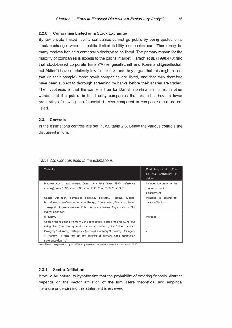
25

2.2.8. Companies Listed on a Stock Exchange By law private limited liability companies cannot go public by being quoted on a stock exchange, whereas public limited liability companies can. There may be many motives behind a company's decision to be listed. The primary reason for the majority of companies is access to the capital market. Harhoff et al. (1998:470) find that stock-based corporate firms ("Aktiengesellschaft and Kommanditgesellschaft auf Aktien") have a relatively low failure risk, and they argue that this might reflect that (in their sample) many stock companies are listed, and that they therefore have been subject to thorough screening by banks before their shares are traded. The hypothesis is that the same is true for Danish non-financial firms, in other words, that the public limited liability companies that are listed have a lower probability of moving into financial distress compared to companies that are not listed.

2.3. Controls In the estimations controls are set in, c.f. table 2.3. Below the various controls are discussed in turn.

Table 2.3: Controls used in the estimations

Variables Control/expected effect

on the probability of

default

Macroeconomic environment (Year dummies): Year 1996 (reference

dummy), Year 1997, Year 1998, Year 1999, Year 2000, Year 2001

Included to control for the

macroeconomic

environment

Sector Affiliation dummies: Farming, Forestry, Fishing, Mining,

Manufacturing (reference dummy), Energy, Construction, Trade and hotel,

Transport, Business service, Public service activities, Organisations, Not

stated, Unknown

Included to control for

sector affiliation

IT dummy Increase

Some firms register a Primary Bank connection in one of the following four

categories (see the appendix on data, section , for further details):

Category 1 (dummy), Category 2 (dummy), Category 3 (dummy), Category

4 (dummy), Firm’s that do not register a primary bank connection

(reference dummy)

?

Note: There is no year dummy in 1995 as, by construction, no firms leave the database in 1995.

2.3.1. Sector Affiliation It would be natural to hypothesize that the probability of entering financial distress depends on the sector affiliation of the firm. Here theoretical and empirical literature underpinning this statement is reviewed.


26

In a theoretical model Gort and Klepper (1982) show that technological and knowledge conditions determine the relative ease with which new firms are able to innovate and therefore survive. Audretch (1991), who studies the survival rates at the industry level, tests the model and finds that survival rates vary considerably across industries, and that they are shaped by the conditions of technology and demand underlying the industry. Audretch and Mahmood (1995) take the analysis a step further and identify explicitly the post-entry performance of new businesses by linking their likelihood of survival to the conditions of technology and demand underlying the industry within which they operate. They find that the likelihood of a new business surviving is in fact shaped by the underlying technological conditions and extent of scale economics among other things. The empirical evidence in Agarwal and Audretsch (2001) also suggests that the relationship between firm size and the likelihood of survival is shaped by technology and the stage of the industry life cycle.

The hypothesis is that the probability of moving into financial distress varies between different business sectors, and so dummies for sector affiliation are used in the estimations. The division of companies into the various sectors follows the NACE classification. As there is no NACE sector affiliation category called "IT and telecommunication companies" a dummy variable is constructed after the other dummies are specified. For details of how the dummies are constructed the reader is referred to the appendix on data (section 9).

2.3.2. Macroeconomic Effects Several studies have found that business cycle effects influence movements in and out of financial distress, e.g. Audretsch and Mahmood (1995), who among other things examine the link between the business cycle and the exposure to risk by including the unemployment rate. They find a positive coefficient of the unemployment rate, which suggests that the hazard rate for new establishments tends to be greater during periods of higher unemployment (which is commonly associated with macroeconomic downturns). In line with Audretsch and Mahmood (1995) our hypothesis is that macroeconomic downturns increase the likelihood of moving into financial distress. In the estimations, year dummies are included to control for the macroeconomic environment. They affect all the firms in the same way and they serve as a robust control for common aggregate effects. Any aggregate variable will be a linear combination of the time dummies, and thus, if a full set of time dummies is included any aggregate variable will be perfectly co-linear with them and hence redundant, as is discussed in Arellano (2003:61). Note that in this paper only estimations of the aggregate process are estimated. The actual process is not specified. This is the best that can be done with a small T panel.


27

2.3.3. Firms with a Primary Bank Some firms register their primary bank connection. If the fact that the firms register a primary bank can be thought of as relationship lending, then the fact that a firm registers a bank under “primary bank” can be interpreted as a more outspoken banking relationship compared to the relationships of the firms that do not register a primary bank. In line with the paper of Brito and Mello (1995), presented in box 2.1.3, the hypothesis would be that the firms that register a primary bank have a lower probability of moving into financial distress. Here, no hypothesis is set up. It is not clear whether there is an effect of a registration of a primary bank on the probability of moving into financial distress. In the estimations, the banks are split up according to the four categories 1, 2, 3 and 4, based on the volume of working capital of the banks (working capital comprises deposits, issued bonds, subordinate capital, and equity capital), c.f. the data description in the appendix on data (section 9).

3. Data and the Construction of the Dependent Variable In this section data is presented, and the construction of the dependent variable is discussed. In the first section on data an introduction to the database is given, the sample selection procedure is presented, and special issues concerning duration data is discussed. Then a thorough discussion of the construction of the dependent variable follows, and an overview of the data set is given.

3.1. The Data Base and Sample Selection Data is obtained from the credit-rating agency KOB A/S. The data base covers all Danish public limited liability companies (“aktieselskaber”) and private limited liability companies (“anpartsselskaber”) that existed in the period from 1995 to 2001. The data set consists of a single spell for each firm. Once a firm has exited it cannot re-enter. This type of data is called duration data.

Duration data can be either flow or stock sampled (Wooldridge (2002:chapter 20)). Flow sampling occurs when individuals or firms, that enter the state of interest at some point during an interval, are sampled, whereas stock sampling occurs when only individuals or firms, that are in the initial state at a given point in time, are sampled. The present data is a combination of stock- and flow-sampled data. The firms that were incorporated before 1995 but only observed since 1995 are stock sampled, since the firms are only observed between 1995 and 2001 no matter when they were incorporated. The new firms entering between 1995 and 2001 are flow sampled. An event is censored if the exact time at which the event occurs is not observed. Both flow- and stock-sampled data can be right censored, whereas only stock-sampled data can be left censored or left truncated, see D’Addio and


28

Rosholm (2002: 4ff).10 In the data set, if the firms have not exited before 2001, they are right censored. There is no left censoring as the incorporation date of all companies is known, however, the stock sampled spells are left truncated as the spells are in progress when the observation period starts. The flow sampled spells are not left truncated as they start at some point “in the observation window” (i.e. between 1995 and 2001), c.f. box 3.1.

Box 3.1: 5 different firms (examples of spells)

10

Right censoring refers to the situation where there is missing information on the times and states occupied after the end of a given observation period. Left censoring refers to the situation where a spell is in progress at the beginning of the observation period and where only the duration from that point in time is observed. Left truncation refers to a situation where a spell is in progress at the beginning of the observation period and where the duration from that point in time is observed and where at the same time the origin date is known. The important difference between left censoring and left truncation is that when a spell is left censored, the origin date of the spell in progress at the start of the observation period is unknown, whereas when a spell is left truncated the origin date of the spell in progress at the start of the observation period is known.

OBSERVATION WINDOW

No. 1 …

No. 2

No. 3

No. 4

No. 5

…. 1993 1994 1995 1996 1997 1998 1999 2000 2001 2002 2003 …

Five different representative firms from the dataset are sketched. The observation window covers the period 1995 to 2001. Spell no. 2 and 5 represent stock sampled spells, whereas spell no. 1, 3 and 4 represent flow sampled spells. The firms in the box are censored in various ways. Firm no. 3 is not censored at all. The spell is complete as the full length of the spell is observed. Firm no. 4 is right censored as the firm is not observed beyond 2001. It is neither left censored nor left truncated as the firm is observed from the incorporation date. Firm no. 5 would have been left censored had the starting data not been known. However, the starting date is known and the firm is left truncated. It is also right censored. Firm no. 2 is left truncated and not right censored (as the spell ends in 2001). Firm no. 1 is right censored in 2001.


29

The data base comprises information on financial issues as well as non-financial issues. KOB A/S receives annually accounts data and information on the status of the companies from the Danish Commerce and Companies Agency. The companies are classified as active and inactive firms, respectively. As will be discussed in section 3.2, the inactive firms can be firms that are financially distressed (e.g. firms that have gone bankrupt), voluntarily liquidated firms, or firms that have merged with other firms, etc. At least once a year, KOB A/S conducts a telephone interview with each of the companies to confirm and supplement the accounts data with information on number of employees, sector affiliation, etc. On top of this information received from KOB A/S, new information is incorporated in the data base. The data base is augmented to also include whether or not the company is 1) an ultimate parent company, 2) a wholly owned subsidiary, 3) quoted on the stock exchange, 4) owned by the public, 5) owned by a fund and 6) a concentration index (measuring the concentration of the various sectors).11

In the raw data set there are 603,956 firm-year observations covering the period 1995-2001. After the exclusion of holding companies and financial firms and after making some corrections to the data base12, there are 430,422 firm-year observations left. Firms with illogical variables are excluded (such as short-term debt less than zero and a solvency ratio larger than 100 per cent) and remaining are 409,906 firm-year observations. A panel is then constructed.

The panel comprises: 1) companies incorporated in the period 1995-2001 with at least 5 employees the year they are included in the sample and with a balance sheet of at least kr. 500,000 (the flow sampled companies), 2) companies that were active in 1995 but were incorporated before 1995 (the stock sampled companies) with a balance sheet of at least kr. 500,000 and 5 employees in 1995.

11

Kasper Nielsen has helped me with information on items 1), 2), 4) and 5). The Danish Competition Authority has kindly provided the concentration index.

12 The financial statement for a specific firm is deleted if it is not the last financial statement for the

company in a specific year in order to insure that there is only one financial statement from each company each year. Furthermore, the company is deleted from the database, if 1) it has had a net return on assets above 300 pct. (or below -300 per cent) in one specific year, if 2) the company is financially distressed in 1995 (so that there is not a financial statement from it when it can be classified as an active company), if 3) the company does not hand in a financial statement each year, if 4) it has a solvency ratio less than -100 pct. and if 5) the company is assessed not to be relevant for the analysis, e.g. A/S Storebæltsforbindelsen, which is a government-guaranteed entity. Government-guaranteed entities are typically structured as government-owned limited-liability companies. Their tasks are defined in an act or legal document, which gives access to government guarantees for loans within a certain limit, c.f. Danmarks Nationalbank (2003:chapter 7.5).


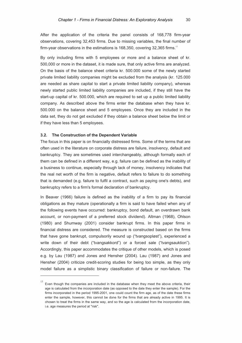
30

After the application of the criteria the panel consists of 168,778 firm-year observations, covering 32,453 firms. Due to missing variables, the final number of firm-year observations in the estimations is 168,350, covering 32,365 firms.13

By only including firms with 5 employees or more and a balance sheet of kr. 500,000 or more in the dataset, it is made sure, that only active firms are analyzed. On the basis of the balance sheet criteria kr. 500.000 some of the newly started private limited liability companies might be excluded from the analysis (kr. 125.000 are needed as share capital to start a private limited liability company), whereas newly started public limited liability companies are included, if they still have the start-up capital of kr. 500.000, which are required to set up a public limited liability company. As described above the firms enter the database when they have kr. 500.000 on the balance sheet and 5 employees. Once they are included in the data set, they do not get excluded if they obtain a balance sheet below the limit or if they have less than 5 employees.

3.2. The Construction of the Dependent Variable The focus in this paper is on financially distressed firms. Some of the terms that are often used in the literature on corporate distress are failure, insolvency, default and bankruptcy. They are sometimes used interchangeably, although formally each of them can be defined in a different way, e.g. failure can be defined as the inability of a business to continue, especially through lack of money, insolvency indicates that the real net worth of the firm is negative, default refers to failure to do something that is demanded (e.g. failure to fulfil a contract, such as paying one's debts), and bankruptcy refers to a firm's formal declaration of bankruptcy.

In Beaver (1966) failure is defined as the inability of a firm to pay its financial obligations as they mature (operationally a firm is said to have failed when any of the following events have occurred: bankruptcy, bond default, an overdrawn bank account, or non-payment of a preferred stock dividend). Altman (1968), Ohlson (1980) and Shumway (2001) consider bankrupt firms. In this paper firms in financial distress are considered. The measure is constructed based on the firms that have gone bankrupt, compulsorily wound up (“tvangsopløst”), experienced a write down of their debt (“tvangsakkord”) or a forced sale (“tvangsauktion”). Accordingly, this paper accommodates the critique of other models, which is posed e.g. by Lau (1987) and Jones and Hensher (2004). Lau (1987) and Jones and Hensher (2004) criticize credit-scoring studies for being too simple, as they only model failure as a simplistic binary classification of failure or non-failure. The 13

Even though the companies are included in the database when they meet the above criteria, their age is calculated from the incorporation date (as opposed to the date they enter the sample). For the firms incorporated in the period 1995-2001, one could count the firm age, as of the date these firms enter the sample, however, this cannot be done for the firms that are already active in 1995. It is chosen to treat the firms in the same way, and so the age is calculated from the incorporation date, i.e. age measures the period at "risk".


31

approach is called into question, as the strict legal concept of bankruptcy may not always reflect the true underlying economic reality of corporate financial distress. The construction of the dependent variable, which is used in this paper, is now discussed in detail.

In the data base, the companies are split up on the ones that are active and inactive. The inactive firms can exit the data base for various reasons: They can go bankrupt, they can be compulsorily wound up, they can be voluntarily liquidated and they can merge, etc. with other companies. The basis for these first three registrations in the database is the registrations in the official documents “Registreringstidende” and “Statstidende” (more on this below). Whether or not the company has merged with other companies, or it has exited for other reasons, is registered by KOB A/S. The active firms are registered if they have had their debt written down or if they have experienced a forced sale. By construction, the active firms that have experienced a write-down of their debt or a forced sale do not appear in the database after these events.

The registrations of the firms that have gone bankrupt, the firms that have been compulsorily wound up and the firms that have been voluntarily liquidated are the responsibility of the Danish Ministry of Economic and Business Affairs.14 A firm has a bankruptcy code if it has formally been declared or if it is in the process of being declared bankrupt. To be compulsorily wound up means, that the Danish Commerce and Companies Agency has closed or decided to close the company. This can happen in situations where a company does not meet the legal requirements, e.g. when a company has not handed in its financial statement. Often it is financially distressed firms that do not fulfil the legal requirements (Møller et al. (1998:318f)). A firm is voluntarily liquidated when the owner of a firm decides to close down the business. In this situation the creditors are paid, and the firm is then closed. This could happen in family-owned firms, when there is no new generation to take over, e.g. because of retirement or death. It is central to note, that firms that are voluntarily liquidated do not inflict losses on their creditors. A discussion of voluntary and involuntary exits is found in Phillips and Kirchhoff (1989:67f), although they end up not distinguishing between forms of exit in their estimations. They focus on the survival of firms, which "needs no further definitional refinement" (Phillips and Kirchhoff (1989:68)).

The focus in this paper is on the firms that end up in financial distress, or in other words, firms that can be expected to inflict a loss on the financial sector. In the measure of financially distressed firms the following firms are included: firms that

14 In practice, the Danish Commerce and Companies Agency, which is under the auspices of the

Danish Ministry of Economic and Business affairs, takes care of the administration of company and enterprise legislation, the registration and disclosure of certain information and documents about companies, including company accounts, etc.


32

have gone bankrupt, firms that have been compulsorily wound up and firms that have experienced a write down of their debt or a forced sale. The firms in financial distress are referred to as E1 firms. The firms that leave the data base for other reasons include firms that have been voluntarily liquidated (E2 firms) and firms that have exited because of a merger or acquisition (E3 firms). By construction, all exits are equal to E1+E2+E3.

Figure 3.2.a: A firm's last financial statement and the registration of the codes

Table 3.2.a: Number of firms

E1 E2 E3 Active Total

1995 0 0 0 18853 18853

1996 372 87 177 20684 21320

1997 348 110 156 22008 22622

1998 347 129 195 23422 24093

1999 453 124 211 25000 25788

2000 618 148 226 26415 27407

2001 479 309 268 27639 28695

Total 2617 907 1233 164021 168778

Note: The number of firms that exit because of financial distress is 479 in 2001. This figure might be a little lower than the “actual” number. As was mentioned above, it takes time before the firms get the codes from the Danish Commerce and Companies Agency. The last information on the firms in the data set was incorporated in spring 2003. The data set covers firms that have handed in their financial statement in 2001 at the latest. If a potential bankrupt firm has not yet got the bankruptcy code in spring 2003 (but might have got it in fall 2003), it will not be recorded as a bankrupt firm in the data set. There could be a few firms for which this would be the case, and therefore the “actual” number of firms entering financial distress in 2001 is probably higher (and for sure not smaller) than the recorded number 479. The sample, which is used in the estimations, entails a slightly smaller number of firms, as firms with missing values on any of the explanatory variables are excluded.

active active no inform. bankruptcy code : Raw data active bankrupt "real bankruptcy" N.A. : Data set recorded as the day after the firm hands in its last financial statement

1995 1996 no inform. 14th September 1997 fin. statem. fin. statem. no inform. no inform.


33

There is a lag between a firm's last financial statement and the registration of the codes (bankruptcy, compulsorily winding-up, voluntarily liquidated etc.). Take the example of a bankrupt firm. The timing of events could follow the time line sketched in figure 3.2.a. According to the raw data, the firm is active in 1995 and in 1996, and it hands in a financial statement both years. In September 1997 the firm gets a bankruptcy code from the Danish Commerce and Companies Agency. Apart from the code there is no further information on the firm in September 1997. The amount of time that passes by between the company hands in its last financial statement in 1996 and till it gets, in this case, the bankruptcy code, is arbitrary. It depends on the bankruptcy court that handles the specific case (how many cases it has already, etc). For this reason the data set is constructed so that the day after the last financial statement is handed in is recorded as the "actual" time of the bankruptcy. The way to treat data is consistent with other credit-scoring studies, e.g. Ohlson (1980) and Jones and Hensher (2004), which also use the published annual report, which is prior to the announcement of failure.

Table 3.2.a shows the number of active firms every year and the number of firms that exit for E1, E2 and E3 reasons. The change in number of active firms is not equal to the number of exits as new firms enter the data base every year. Most of the firms that exit the data base, exit because of financial distress. Voluntary liquidations account for the smallest number of exits.

The trend in the number of firms that leave the data set follows, with a lag, the trend in the number of official bankruptcies in the period 1995-2001, c.f. figure 3.2.b. The lag between e.g. the peak of the firms in financial distress in mid-2000 and the peak of the bankruptcies in the beginning of 2002 is due to the timing issues discussed above (in connection with figure 3.2.a). On average this lag is 1.5 years, c.f. figure 3.2.b.

In the database, a firm in financial distress is registered, when it hands in its last financial statement. The bankruptcy figures from Statistics Denmark show the bankruptcies at the actual date of the bankruptcy. The difference in levels between the firms in financial distress and the bankruptcies is mainly due to the facts 1) that the database entails only public and private limited liability companies, whereas the figure from Statistics Denmark also includes sole proprietorships etc., and 2) that there is no sample selection behind the figures that Statistics Denmark report, whereas the database e.g. is restricted to only include firms with 5 employees and a total balance sheet of kr. 500.000 the year they are included in the dataset.


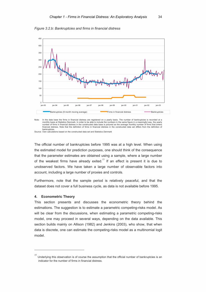
34

Figure 3.2.b: Bankruptcies and firms in financial distress

0

50

100

150

200

250

300

350

400

450

jan-93 jan-94 jan-95 jan-96 jan-97 jan-98 jan-99 jan-00 jan-01 jan-02 jan-03

Bankruptcies (9 month moving average) Firms in financial distress Bankruptcies

Note: In the data base the firms in financial distress are registered on a yearly basis. The number of bankruptcies is recorded at a

monthly basis at Statistics Denmark. In order to be able to include the numbers in the same figure in a meaningful way, the yearly number of firms in financial distress in the constructed data base is pictured as the average monthly number of firms that enters financial distress. Note that the definition of firms in financial distress in the constructed data set differs from the definition of bankruptcies.

Source: Own calculations based on the constructed data set and Statistics Denmark

The official number of bankruptcies before 1995 was at a high level. When using the estimated model for prediction purposes, one should think of the consequence that the parameter estimates are obtained using a sample, where a large number of the weakest firms have already exited.15 If an effect is present it is due to unobserved factors. We have taken a large number of observable factors into account, including a large number of proxies and controls.

Furthermore, note that the sample period is relatively peaceful, and that the dataset does not cover a full business cycle, as data is not available before 1995.

4. Econometric Theory This section presents and discusses the econometric theory behind the estimations. The suggestion is to estimate a parametric competing-risks model. As will be clear from the discussions, when estimating a parametric competing-risks model, one may proceed in several ways, depending on the data available. This section builds mainly on Allison (1982) and Jenkins (2003), who show, that when data is discrete, one can estimate the competing-risks model as a multinomial logit model.

15 Underlying this observation is of course the assumption that the official number of bankruptcies is an

indicator for the number of firms in financial distress.


35

As the competing-risks model is estimated as a multinomial logit model, two specification tests for multinomial logit models are presented here (and performed in section 5). The first is the test for the independence of irrelevant alternatives (IIA assumption). The second is a test for pooling states in the multinomial logit model.

4.1. Competing-risks model The firms leave the data base for E1, E2 and E3 reasons. The occurrence of one type of event removes the firm at risk of all other event types, and so the method of competing-risks models is to be considered. Formally competing-risks models can be characterized in the following way, c.f. Jenkins (2003:75f): Let )(1 thE be the hazard rate of exit to financial distress, i.e. the probability that the firm exits as an E1 firm given that it made it to the period (with the latent failure time 1T ), let

)(2 thE be the hazard rate of exit to voluntary liquidation (with the latent failure time

2T ) and )(3 thE be the hazard rate of exit to mergers, acquisitions etc. (with the latent failure time 3T ). It is observed in the data whether there is no event at all (a censored case corresponding to an active firm, with spell length 4T ), or whether there is an E1, E2 or E3 exit. Therefore the observed failure time is

},,,min{ 4321 TTTTtimeT = .

Table 4.1: Grouped duration data and the five main assumptions in the literature

Main assumption Main implications

Transitions can only occur at the boundaries of the intervals

Same result as in the continuous case (where the overall independent competing risk model can be estimated by estimating separate destination-specific models).

Destination-specific density functions are constant within each interval (though may vary between intervals)

The expression for the likelihood contribution is not separable into destination-specific competing-risk models.

Destinations specific hazard rates are constant within each interval (though may vary between intervals)

The expression for the likelihood contribution is not separable into destination-specific competing-risk models.

The hazard rate takes a particular proportional hazards form

This might be thought of as a more flexible specification of the hazard function. However note that it cannot be identified without further assumptions.

The log of the integrated hazard changes linearly over the interval

This estimation procedure, which is rather complicated, has been used relatively rarely.

Source: Jenkins (2003: chapter 8).

When estimating a competing-risks model one can follow several estimation strategies depending on the data at hand, c.f. Jenkins (2003:75ff). With continuous data and the assumption of independent exits each destination-specific hazard rate can be thought of as the hazard rate that would apply were transitions to all the other destinations not possible, and one can maximize the overall log likelihood by


36

maximizing the component parts separately. In practice, this can be done very easily. One should simply define new destination-specific censoring variables and then estimate separate models for each destination state.

With grouped duration data one can assume that the durations are intrinsically discrete and treat them accordingly. Alternatively one may attempt to relate the model to an underlying process in continuous time. If one chooses the first option, one can use a "trick" demonstrated in Allison (1982). He shows that by assuming independent exits and a particular form of destination-specific hazards, the likelihood has the same form as the likelihood for a standard multinomial logit model (more on this below). If one chooses the second option, things get more complicated as the shape of the continuous time hazard rate within each interval cannot be identified from the available grouped data. On top of the assumption of independent exits, the construction of the sample likelihood requires then assumptions about the shape of the continuous time hazard rate. Alternative assumptions lead to different econometric models. Jenkins (2003:chapter 8) has a detailed overview (with derivations) of some of the various estimation strategies that have been attempted in the literature. Table 4.1 summarizes his discussions.

The approach taken here is to treat the data as if they were discrete, thereby eschewing any attempt to relate the model to an underlying process in continuous time, c.f. the estimation strategy in Allison (1982). Following Allison (1982) and Jenkins (2003) the way to proceed is to start off by assuming that the exits are independent of each other. The assumption of independent exits implies that the overall likelihood contribution for a firm can be written in the following way:

321321 1321 )()()()( EEEEEE

activeEEE LLLLL δδδδδδ −−−=

21

)()()(1)(

)()()(1)(

321

2

321

1EE

thththth

thththth

EEE

E

EEE

E

δδ

⎥⎦

⎤⎢⎣

⎡−−−⎥

⎦

⎤⎢⎣

⎡−−−

=

∏=

−−−×⎥⎦

⎤⎢⎣

⎡−−−

×t

EEEEEE

E hhhththth

th E

1321

321

3 )]()()(1[)()()(1

)( 3

τ

δ

τττ

where τ denotes the year the firm gets incorporated (this of course differs across firms), and where 1Eδ = 1 when the specific firm exits because of E1, 2Eδ = 1 when the specific firm exits because of E2, and 3Eδ = 1 when the specific firm exits because of E3. When the firm does not exit for E1, E2 or E3 reasons, it is active (and gets censored in 2001).

Even though independent exits are assumed, the discrete-time likelihood cannot be factored into separate components for each of the three events, as it could, for example, in the continuous case. Maximum likelihood estimation must be done simultaneously for all kinds of events. It turns out, that by assuming that the


37

destination-specific hazards have a particular form, there is still a straightforward way of estimating this independent competing-risks model, as the likelihood function can then be rewritten to have the same form as a standard multinomial logit model. This is shown in Allison (1982). Following Allison (1982) and Jenkins (2003) it is assumed that the destination-specific hazards are of the form

)'exp()'exp()'exp(1)'exp(

)(321

11

tEtEtE

tEE XXX

Xth

ββββ

+++=


)(321

22

tEtEtE

tEE XXX

Xth

ββββ

+++=


)(321

33

tEtEtE

tEE XXX

Xth

ββββ

+++=

and so

)'exp()'exp()'exp(11

)()()(1

321

321

tEtEtE

EEE

XXX

ththth

βββ +++=

−−−

where tX characterizes the covariates, which may be time-varying, and β are the parameters of the covariates. The covariates, which are included in the estimations, are the core, proxy and control variables, which are listed in section 2. Age (the baseline-hazard function), which is one of the core variables, can be specified parametrically or non-parametrically. A non-parametric specification is preferred as any inconsistency caused by misspecification is then avoided. In the estimations, dummies for each age (up to a dummy with companies that are 30 years old or older) are included. The reference category is firms that are 1 year old. For the financially distressed firms, the E1 firms, the specification of the baseline-hazard function could be denoted 1' EtD γ where tD would denote the dummies, which are a subset of tX , and 1Eγ would be a subset of the coefficients to be estimated, i.e. a subset of 1Eβ .

The expressions for the destination-specific hazards are inserted in the overall likelihood contribution for a specific firm, and the same form as the likelihood for a standard multinomial logit model is obtained. The likelihood is then:


38

∏−

=

−−−

+++×

⎥⎦

⎤⎢⎣

⎡+++

×

⎥⎦

⎤⎢⎣

⎡+++

×

⎥⎦

⎤⎢⎣

⎡+++

×

⎥⎦

⎤⎢⎣

⎡+++

=

1

1 321

1

321

321

3

321

2

321

1






321

3

2

1

t

EEE

tEtEtE

tEtEtE

tE

tEtEtE

tE

tEtEtE

tE

XXX

XXX

XXXX

XXXX

XXXX

L

EEE

E

E

E

τ τττ

δδδ

δ

δ

δ

βββ

βββ

ββββ

ββββ

ββββ

It is chosen to set the censored firms (the active firms) as the reference category.16

Left truncation and right censoring is handled as in Jenkins (1995), Henley (1998:418) and Rommer (2005b).

The coefficients reported in the appendix on figures and tables (section 10) are interpreted as contrasts between pairs of categories, c.f. the equations below, which are the ones that are actually estimated in the multinomial logit model:

tEactive

E Xhh

11 ')log( β=

tEactive

E Xhh

22 ')log( β=

tEactive

E Xhh

33 ')log( β=

This means for example that in the competing-risks model the odds that a private limited liability company will enter financial distress rather than staying active are about exp(0.4174)=1.52 the odds for public limited liability companies. For the solvency ratio which has exp(-2.5103)=0.08, each 1-level increase in the variable multiplies the odds of moving into financial distress versus staying active by about

16

When estimating a multinomial logit model, one must be aware of the identification issue. The m alternative choices (E1, E2, E3 and being censored) cannot be identified, as there is more than one set of estimates that would lead to the same probabilities of the outcomes observed. The way to deal with this problem is to set one of the sets of parameters equal to zero.


39

0.08. More details on the interpretation of the coefficients in the multinomial logit model are found in section 6.1.

The estimated model is called an independent competing-risks model, as the correlations between unobservable factors affecting each destination-specific hazard are assumed away. To account for potential unobserved characteristics in the multinomial logit model, unobserved heterogeneity can be introduced (see e.g. Malchow-Møller and Svarer (2002)). Unobserved heterogeneity is not introduced here. Instead of including unobserved heterogeneity, proxy variables are included in the estimations, as is discussed in section 2.2. This approach is in line with Jenkins (2003:102), who notes, that the effects of unobserved heterogeneity are mitigated, and thence estimates are more robust, if a flexible baseline-hazard specification is used (as it is in this case), and that the topic of unobserved heterogeneity underscores the importance of getting good data, including a wide range of explanatory variables that summarize well the differences between, in this case, the firms. This means that if one has a wide range of explanatory variables, it is less of a problem not to control for unobserved heterogeneity.

4.2. Independence of Irrelevant Alternatives The fact that the multinomial logit coefficients always must be interpreted as effects on contrasts between pairs of categories and not on the probability of being in a particular category is often referred to as “relative risk” or as the assumption of “independence of irrelevant alternatives” (IIA). The assumption implies that adding another alternative (or changing characteristics of another alternative) does not affect the relative odds between two of the alternatives. The IIA assumption is implausible for applications with similar alternatives. Wooldridge (2002) and Train (2003) consider the well-known red bus/blue bus example, where adding a blue bus to the choice set of taking the train or the red bus, changes the probability of taking the train, even though the probability of taking the train should be the same as before and not depend on the new choice. The simple example is this: first there is the choice of taking a red bus or the train instead of a car. Say, that the estimated probability of taking the red bus/car is one half and so is the train/car probability. Now, a new alternative is added, e.g. a blue bus. The IIA property implies that the relative odds between taking the red bus and the train are the same as before. The new probabilities will then be the following: the probability of taking the blue bus/car is one third, the red bus/car is one third and also that the probability of taking the train/car is one third (note that the relative odds between taking the red bus and the train would not be changed). But this makes no sense. It should not matter whether the bus is red or blue. It would be more realistic if the probability of taking the train/car was still one half, and then the probability of taking the red bus/car and blue bus/car were both, one fourth.


40

The potential problem sketched in the example, is not something to worry about in

the problem of interest in this paper. Here the alternatives E1, E2 and E3 are not

similar, and so, a priori, there should be no reason to believe that one category

could be excluded. Nonetheless, to be sure, it is chosen to test the assumption of

independence of irrelevant alternatives. The assumption can be tested with

Hausman’s specification test. If “a subset of the choice set truly is irrelevant,

omitting it from the model altogether will not change parameter estimates

systematically. Exclusion of these choices will be inefficient but will not lead to

inconsistency. But if the remaining odds are not truly independent of these

alternatives, then the parameter estimates obtained when these choices are

included will be inconsistent” (Greene (2003:725)).17 Franses and Paap (2001:97)

explain: “The idea behind the test is that deleting one of the categories should not

affect the estimates of the remaining parameters if the IIA assumption is valid. If it

is valid, the estimation of the odds of two outcomes should not depend on

alternative categories. The test amounts to checking whether the difference

between the parameter estimates based on all categories and the parameter

estimates when one or more categories are neglected is significant.”

The test statistic is ^ ^ ^ ^ ^ ^

2 1( ) '[ ] ( )s fs f s fV Vχ β β β β−= − − − , where s indicates the

estimators based on the restricted subset and f indicates the estimator based on

the full set of choices, and ^

V are the estimates of the asymptotic covariance

matrices. The statistic has a limiting chi-squared distribution with K degrees of

freedom, where K is the number of parameters to be tested. The IIA assumption is

tested and the result is reported in section 5.

4.3. Pooling States in the Multinomial Logit Model Another relevant specification test is to test for the pooling of states in the multinomial logit model. It is an empirical question whether a subset of states can be treated as a single state, or whether they show significant differences. A test for the pooling of states is presented and discussed in Cramer and Ridder (1991) and in Franses and Paap (2001). Below the test is explained in a situation, where two states are pooled. This is an example of how to perform the test. The method can also be used in applications, where the pooling of more than two states is of interest.

17 As an aside, note, that if one estimates a binary logit model with bankrupt and active firms only

instead of a multinomial logit model where the exits to all states are specified, the coefficients are consistent, but less efficient than in the multinomial logit model, c.f. Begg and Grey (1984).


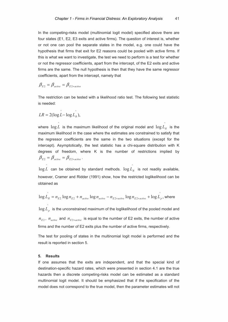
41

In the competing-risks model (multinomial logit model) specified above there are four states (E1, E2, E3 exits and active firms). The question of interest is, whether or not one can pool the separate states in the model, e.g. one could have the hypothesis that firms that exit for E2 reasons could be pooled with active firms. If this is what we want to investigate, the test we need to perform is a test for whether or not the regressor coefficients, apart from the intercept, of the E2 exits and active firms are the same. The null hypothesis is then that they have the same regressor coefficients, apart from the intercept, namely that

activeEactiveE +== 22 βββ

The restriction can be tested with a likelihood ratio test. The following test statistic is needed:

,)log(log2^^

RLLLR −=

where ^

log L is the maximum likelihood of the original model and ^

log RL is the maximum likelihood in the case where the estimates are constrained to satisfy that the regressor coefficients are the same in the two situations (except for the intercept). Asymptotically, the test statistic has a chi-square distribution with K degrees of freedom, where K is the number of restrictions implied by

activeEactiveE +== 22 βββ .

^

log L can be obtained by standard methods. ^

log RL is not readily available,

however, Cramer and Ridder (1991) show, how the restricted loglikelihood can be

obtained as

,logloglogloglog^

2222

^

pactiveEactiveEactiveactiveEER LnnnnnnL +−+= ++ where

^log pL is the unconstrained maximum of the loglikelihood of the pooled model and

2En , activen and activeEn +2 is equal to the number of E2 exits, the number of active

firms and the number of E2 exits plus the number of active firms, respectively.

The test for pooling of states in the multinomial logit model is performed and the

result is reported in section 5.

5. Results If one assumes that the exits are independent, and that the special kind of destination-specific hazard rates, which were presented in section 4.1 are the true hazards then a discrete competing-risks model can be estimated as a standard multinomial logit model. It should be emphasized that if the specification of the model does not correspond to the true model, then the parameter estimates will not


42

be consistent. Note that the assumption of independent exits is necessary for identification, and that it therefore cannot be tested.

The results from the estimation of the competing-risks model are presented in this section, and specification tests are performed.

Other papers, which use the same estimation approach, though, in other contexts, are Fahrmeier and Wagenpfeil (1996) and Henley (1998).

5.1. Specification Tests The specification tests, which were presented in section 4, are performed. First, the IIA assumption is tested. As a start, E2 firms are left out of the estimations. The null hypothesis is that the difference in coefficients between the less efficient estimates obtained from the multinomial logit model without E2 firms and the fully efficient estimates obtained from the multinomial logit model, where all exits are included, is not systematic. The alternative hypothesis is that the difference in coefficients is systematic. If the E2 firms are truly irrelevant, omitting them from the model should not change parameter estimates systematically.

The test statistic is ^ ^ ^ ^ ^ ^

2 1( ) '[ ] ( )s fs f s fV Vχ β β β β−= − − − =6.77 (s indicates the

estimators based on the restricted subset and f indicates the estimator based on

the full set of choices, and ^

V are the estimates of the asymptotic covariance

matrices). The statistic has a limiting chi-squared distribution with 128 degrees of

freedom (equal to the number of parameters to be tested). The 000.1Pr 2 => χ ,

and so the null hypothesis is accepted, indicating that the difference in coefficients

is not systematic. This implies that the IIA specification holds and therefore that E2

firms should not be left out of the estimations. The E1 parameter estimates are

consistent and efficient, when the E2 firms are included in the estimations.

The next step is to leave E3 firms out. When they are left out of the estimations,

the test statistic is ^ ^ ^ ^ ^ ^

2 1( ) '[ ] ( )s fs f s fV Vχ β β β β−= − − − =2.63. Again the statistic has

a limiting chi-squared distribution with 128 degrees of freedom. The

000.1Pr 2 => χ , and so the null hypothesis is accepted, indicating that the

difference in coefficients is not systematic. This implies that the IIA specification

holds and therefore that E3 firms should not be left out of the estimations. The E1

parameter estimates are consistent and efficient, when the E3 firms are included in

the estimations.

The conclusion from the test of the IIA assumption is that when E2 and E3 firms are left out, respectively, the difference in coefficients is not systematic. This


43

implies that the IIA specification holds and therefore that the model is correctly specified when all exit modes are included.

The second specification test is the test for the pooling of states in the multinomial logit model. Shumway (2001) treats firms that exit for other reasons than financial distress as active until they have left the sample (then they are treated as censored or no longer observed). This feature of hazard models is highlighted in Balcaen and Ooghe (2004) who write, that hazard models consider firms that exit for other reasons than financial distress to be censored. They elaborate: “Survival analysis only allows for ‘randomly censored’ case when the random censoring is non-informative. This means that the censoring times do not depend on the failure risk. At moment t, randomly censored firms need to be representative for all firms that have survived up to the moment t with similar values for the independent variables. The failure risk of these ‘randomly censored’ firms is required to be similar to the failure risk of the other, surviving companies” (Balcaen and Ooghe (2004:4)). Lando (2004:81), who discusses statistical techniques for analyzing defaults, writes that in the hazard model we need to think “of this censoring mechanism as being unrelated to the default event. … In the real world, we see nondefaulted firms as part of mergers or target of takeover, and although in some sectors such activity may be related to an increased default probability, it does not seem to be a big problem in empirical work.”

Following the suggestions in Shumway (2001) and Balcaen and Ooghe (2004) to lump E2, E3 and active firms, the interesting specification test, which is reported below, is, whether or not one can pool E2, E3 and active firms. Lando (2004) is less specific, but one could interpret his comments, as if he suggests that E3 and active firms could be lumped together.

In this case, where we want to test whether or not one can pool E2, E3 and active firms, under the null, we have that E2, E3 and active firms have the same regressor coefficients, apart from the intercept.

The sample consists of 168,350 firm-years, split up on the following categories: E1 exits: 2,586, E2 exits: 856, E3 exits: 1,224, active firms: 163,684. The maximum likelihood of the original model with four states, the multinomial logit model, is -20,926. The maximum likelihood of a model with two states, namely E1 exits versus E2, E3 and active firms, is -10,592. From the sample numbers we obtain

activeEEactiveEEactiveactiveEEEE nnnnnnnn ++++−++ 32323322 loglogloglog

= 5,780 + 8,702 + 1,965,140 – 1,992,205 = -12,583

And so we have that


44

^

32323322

^

logloglogloglog

log

pactiveEEactiveEEactiveactiveEEEE

R

Lnnnnnnnn

L

+−++

=

++++

= -12,583 + (-10,592) = -23,175

The sample numbers as well as the values of the maximized likelihood functions gives us now the test statistic, which is

^^

)log(log2 RLLLR −= = 2 ( (-20,926) – (-23,175)) = 4,498.

This test statistic is asymptotically chi-square distributed with 126 degrees of freedom, as we have twice equated 63 coefficients to one another (i.e. all coefficients except the intercept), c.f. the restrictions under the null. The null hypothesis is rejected, and so we conclude, that E2, E3 and active firms cannot be pooled.

The overall conclusion is, that the specification tests show, that the competing-risks model should be specified as a multinomial logit model in which all states are included (neither E2 or E3 exits should be left out according to the IIA test) and where E2 and E3 exits are treated as separate exits (and not lumped together with active firms. This is the result from the test for the pooling of states).

5.2. Parameter Estimates The parameter estimates, which are obtained when the competing-risks model is estimated, are presented in this section. The results on the E1 hazard from the estimation of the coefficients in the parametric competing-risks model are seen from tables 5.2.a and 5.2.b. The appendix on figures and tables (section 10) presents the results for the E2 hazard and the E3 hazard, c.f. tables 10.a and 10.b. Although these results will not be discussed, note that the results on the E1 and E3 hazard deliver different results from the results that Köke (2001) finds (but he also only look at acquisitions, and not mergers and acquisitions etc.). As is mentioned in the introduction, Köke finds that firms "experiencing failure or acquisition are significantly different from surviving firms on a number of firm-specific characteristics, but that the characteristics are similar for failing and acquired firms". We do not find that firms in financial distress and firms that are merged with or acquired by other firms, etc. have the same characteristics (see e.g. the parameter estimates on the solvency ratio and firm size).

Tables 5.2.a and 5.2.b show that in all cases where an effect of a parameter was hypothesized for firms that exit because of financial distress, the parameter estimates have the expected sign when the competing-risks model is estimated.


45

The core and proxy variables, which were expected and estimated to have a negative coefficient, are age, the return on net assets, the solvency ratio, the diversification variables and the wholly-owned subsidiary dummy. A negative sign indicates that the higher these variables are the less likely a firm is to enter financial distress (relative to staying active). In this respect note that the duration dependence is estimated to be almost linear and downward-sloping until the firms reach the age of 15, and from the age of 15 the effect is approximately constant (figure 5.2.a). The variables short term debt to total assets, the private limited liability dummy and the dummy for having critical comments from the auditors were expected and estimated to have a positive sign, indicating that the higher these variables are the more likely a firm is to enter financial distress (relative to staying active).

Two hypothesis of firm size are tested. Hypothesis A is that there exists an optimal firm size. This means that there is a trade-off between being relatively small and relatively large, and therefore that the effect of firm size on the probability of moving into financial distress is nearly U-shaped. Hypothesis B is that the probability of entering financial distress decreases along with an increase in size. Estimations (not reported) show that when (firm size) and (firm size) 2 are included in the estimations, then (firm size) is significant with a negative sign (significance level is below 1 per cent), and (firm size) 2 is significant with a positive sign (significance level is over 3 per cent). Most variables considered in the estimations are significant with a significance level lower than 1 per cent, c.f. tables 5.2.a and 5.2.b. As (firm size) 2 is only significant with a significance level over 3 per cent, this effect is not considered in the final estimations, i.e. as reported in tables 5.2.a and 5.2.b. The results are considered as being in favour of hypothesis B, which is the preferred hypothesis in section 2, namely that firm size has a negative effect on moving into financial distress.

Table 5.2.a: Core variables (E1 parameter estimates)

Variables Estimated effect Expected effect Firm age (dummies) See the text and figure 5.2.a Negative Short term debt to total assets Positive* Positive Return on net assets Negative* Negative Solvency ratio Negative* Negative Firm size Negative* Negative

Note: The variables are significant at the 1 per cent level (indicated by *). There is controlled for the macroeconomic environment and for

the various sectors. In the estimations, farming and forestry is included in the same sector affiliation category, as the data were too sparse otherwise. The same holds for mining, energy and construction. The IT dummy was positive and significant at the 1 per cent level. The primary bank categories have been altered: as the data was too sparse otherwise, firms that register a bank in category 3 or 4 are now in the same group. Only firms that reported a primary bank in category 2 had a significantly larger probability of entering financially distress. The other bank dummies were not significantly different from zero. The dummy for publicly traded companies is not included in the estimations as no publicly traded firms enter financial distress in the period.


46

Figure 5.2.a: Firms in financial distress: duration dependence

-1,6

-1,4

-1,2

-1

-0,8

-0,6

-0,4

-0,2

02 3 4 5 6 7 8 9 10 11 12 13 14 15 16 17 18 19 20 21 22 23 24 25 26 27 28 29 30

age

dum

mie

s

age dummies 5 year moving average

Note: The figure sketches the age dummies (reference dummy is firms that are equal to 1 year old). The last dummy is called 30 years old or older. All the reported dummies are significant at the 5 per cent. level. Most of them are also significant at the 1 per cent level.

For some of the variables a particular sign was not expected. Instead it was left to the estimations to show whether or not the variable was significant, and what sign the parameter has. This was the case for the proxy variables ultimate parent company, owned by a fund, owned by the public sector, local authority group 2, 3, 4 and 5, and for the control variable primary bank group 1, group 2, and group 3 & 4 (the estimates on the control variables are not reported).

The sign of the parameter of the dummy variable ultimate parent company is positive, and so the odds, that an ultimate parent company will enter financial distress relative to staying active compared to companies that are not ultimate parent companies, are higher. The reason for this may be that the ultimate parent companies have a tendency to let the not-so-well-performing subsidiaries drain resources from the group as a whole, including the ultimate parent company, e.g. because of reputational risk.

The effects of fund ownership and public sector ownership are not significant.

All local authority groups, except of local authority group 4, which measures the effect of being situated outside Zealand in other local authorities with 50,000 inhabitants or more, relative to being situated in Copenhagen and Frederiksberg, have smaller odds of moving into financial distress compared to the companies situated in Copenhagen and Frederiksberg (group 1). The parameter estimate on


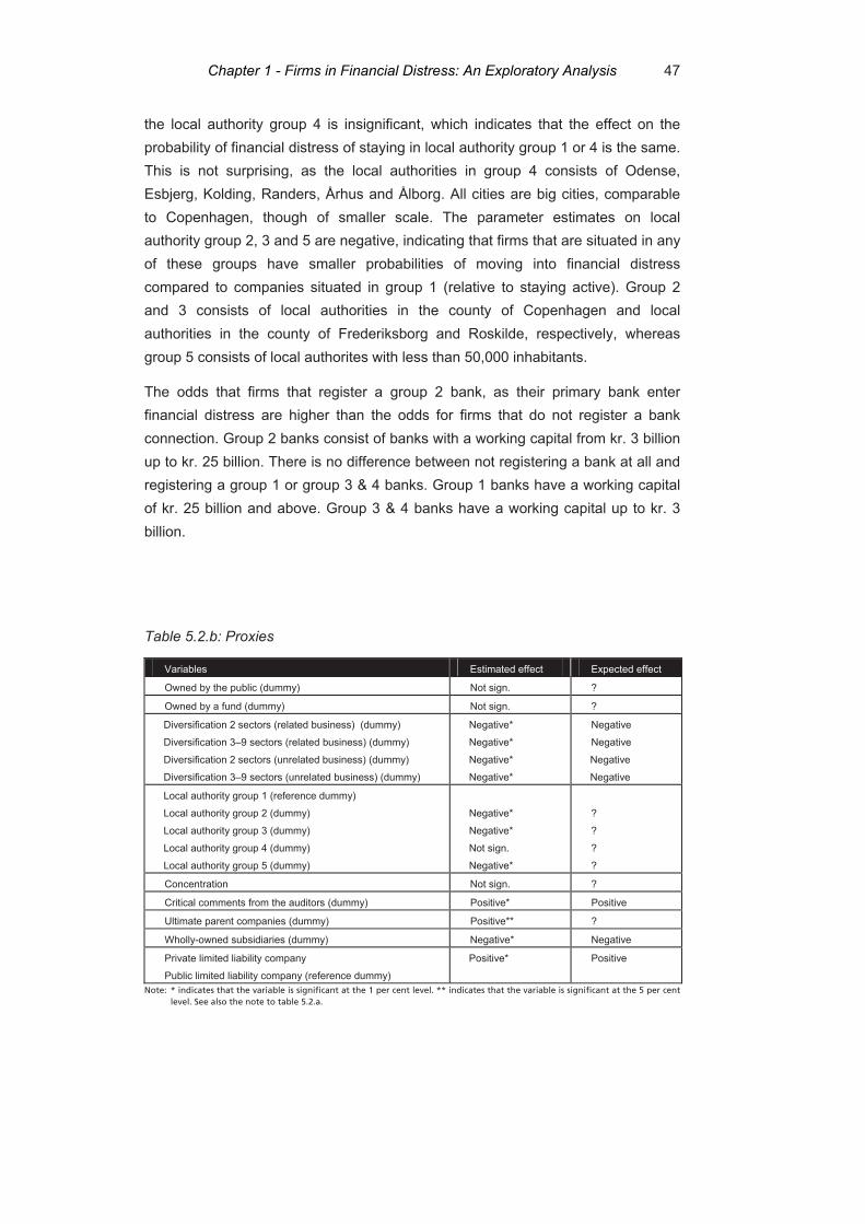
47

the local authority group 4 is insignificant, which indicates that the effect on the probability of financial distress of staying in local authority group 1 or 4 is the same. This is not surprising, as the local authorities in group 4 consists of Odense, Esbjerg, Kolding, Randers, Århus and Ålborg. All cities are big cities, comparable to Copenhagen, though of smaller scale. The parameter estimates on local authority group 2, 3 and 5 are negative, indicating that firms that are situated in any of these groups have smaller probabilities of moving into financial distress compared to companies situated in group 1 (relative to staying active). Group 2 and 3 consists of local authorities in the county of Copenhagen and local authorities in the county of Frederiksborg and Roskilde, respectively, whereas group 5 consists of local authorites with less than 50,000 inhabitants.

The odds that firms that register a group 2 bank, as their primary bank enter financial distress are higher than the odds for firms that do not register a bank connection. Group 2 banks consist of banks with a working capital from kr. 3 billion up to kr. 25 billion. There is no difference between not registering a bank at all and registering a group 1 or group 3 & 4 banks. Group 1 banks have a working capital of kr. 25 billion and above. Group 3 & 4 banks have a working capital up to kr. 3 billion.

Table 5.2.b: Proxies

Variables Estimated effect Expected effect

Owned by the public (dummy) Not sign. ?

Owned by a fund (dummy) Not sign. ?





Negative*

Negative*

Negative*

Negative*

Negative

Negative

Negative

Negative






Negative*

Negative*

Not sign.

Negative*

?

?

?

?

Concentration Not sign. ?

Critical comments from the auditors (dummy) Positive* Positive

Ultimate parent companies (dummy) Positive** ?

Wholly-owned subsidiaries (dummy) Negative* Negative

Private limited liability company


Positive* Positive

Note: * indicates that the variable is significant at the 1 per cent level. ** indicates that the variable is significant at the 5 per cent level. See also the note to table 5.2.a.


48

Figure 5.2.b: Macroeconomic dummies and macroeconomic variables

0

20

40

60

80

100

120

140

160

180

1997 1998 1999 2000 2001

Macro-dummy Change in unemploymentChange in GDP Change in interest rates

Note: The macroeconomic dummies as well as the change in unemployment, the change in GDP and the change in interest rates are normalized with 1997 as the base year (which is set equal to 100).

The dummy variables that control for the sector affiliation in the competing-risks model show that compared to being a manufacturing firm (reference dummy) the odds that the firms that belong to one of the following sectors move into financial distress are smaller: trade and hotel, transport, business service, public service activities, and organizations, etc. On the contrary, the odds that the firms that have the sector affiliation "unknown” move into financial distress are higher. Firms with the other sector affiliations are not significantly different from firms in the manufacturing sector. All firms that are in the self-constructed IT- and telecommunication category have higher odds of moving into financial distress than all other firms.

The macroeconomic dummies as well as macroeconomic variables are sketched in figure 5.2.b. Although the time series is not long enough to make any strong conclusion concerning the macroeconomic effects, one could as a preliminary observation state, that it seems as if the macroeconomic dummies follow the change in unemployment with a two-year lag.


49

5.3. Goodness-of-fit and Robustness The goodness-of-fit of the model can be judged from table 5.3.a. The table tabulates the actual events versus the average predicted probability of the respective events. No cut-off level is chosen. The predicted event is the one with the highest probability. Table 5.3.a should be read in the following way: out of the firms that end up in financial distress (see the "actual E1" column), 10.19 per cent were predicted to end up in financial distress, 1.08 were predicted to end up as voluntarily liquidated, 0.74 were predicted to merge with other companies or the like, and 88 pct. were predicted to be active. Note that all columns sum to 1. Look now at the predicted row: 10.19 per cent of the firms that end up as financially distressed firms were predicted to enter financial distress, 3.4 per cent of the firms that end up as voluntarily liquidated were predicted to enter financial distress, 1.78 per cent of the firms that end up as mergers and the like were predicted to enter financial distress, and 1.39 per cent of the firms that end up as active were predicted to enter financial distress.

The important thing to notice from table 5.3.a is that the diagonal numbers are the largest. This implies that the model can distinguish between the various exits.

Table 5.3.b gives an idea about the robustness over time. As expected, for all estimated periods, the diagonal numbers are the largest. It is notable that the model estimated using the whole period 1995 – 2001 seems to be the “worst” model.

Table 5.3.a: Goodness-of-fit: Competing-risks model

Actual Goodness-of-fit

E1 E2 E3 Active All

E1 0.1019 0.0340 0.0178 0.0139 0.0154

E2 0.0108 0.0800 0.0098 0.0046 0.0051

E3 0.0074 0.0199 0.0360 0.0070 0.0073

Average

predicted

probability

Active 0.8798 0.8661 0.9384 0.9736 0.9723


50

Table 5.3.b: Goodness-of-fit using five different samples


E1 E2 E3 Active All

E1 0.15

0.14

0.12

0.12

0.10

0.05

0.05

0.04

0.04

0.03

0.02

0.02

0.02

0.02

0.02

0.01

0.01

0.01

0.01

0.01

0.01

0.01

0.01

0.02

0.02

E2 0.01

0.01

0.01

0.01

0.01

0.11

0.11

0.10

0.09

0.08

0.01

0.01

0.01

0.01

0.01

0.00

0.00

0.00

0.00

0.00

0.00

0.00

0.00

0.00

0.01

E3 0.01

0.01

0.01

0.01

0.01

0.03

0.03

0.03

0.02

0.02

0.08

0.06

0.05

0.04

0.04

0.00

0.01

0.01

0.01

0.01

0.01

0.01

0.01

0.01

0.01

Average

predicted

probability

Active 0.82

0.84

0.86

0.87

0.88

0.81

0.81

0.83

0.84

0.87

0.89

0.90

0.92

0.93

0.94

0.98

0.98

0.98

0.98

0.97

0.98

0.98

0.98

0.97

0.97

Note: This table pictures the average predicted probability estimated using six different samples. The samples are sketched in the following order: Sample 1995 – 1997 (first line), sample 1995 – 1998 (second line), sample 1995 – 1999 (third line), sample 1995 – 2000 (fourth line) and sample 1995 – 2001 (fifth line).

Table 5.3.c: Goodness-of-fit


E1 E2 E3 Active All

E1 0.07 (0.10) 0.03 (0.03) 0.01 (0.02) 0.01 (0.01) 0.02 (0.02)

E2 0.01 (0.01) 0.04 (0.08) 0.00 (0.01) 0.00 (0.00) 0.01 (0.01)

E3 0.01 (0.01) 0.01 (0.02) 0.01 (0.04) 0.01 (0.01) 0.01 (0.01)

Average

predicted

probability

Active 0.92 (0.88) 0.93 (0.87) 0.97 (0.94) 0.97 (0.97) 0.97 (0.97)

Note: The table shows the average predictions when only the core variables are included in the model. Estimation period is 1995 – 2001. In parenthesis are the predictions when the full set of explanatory variables is used.


51

Some credit-scoring studies are assessing the role of non-financial factors in credit ratings. An example is Grunert, Norden and Weber (2005), who finds that including financial and non-financial factors leads to a more accurate prediction of defaults events. This is also the case for the model set up in this paper, c.f. table 5.3.c, which shows, the consequence of only including the core variables (which also include the non-financial variable age) in the model. When the proxies and the controls are not included in the estimations a smaller number of firms are correctly predicted to experience the E1, E2 and E3 events, respectively.

5.4. Proportion of Correct Predictions The predictive ability of the model is demonstrated by its discriminatory power. As it was chosen to use all the available data in the estimations to have as long a time series as possible, the predictive ability of the model is evaluated in-sample and in-time. Of course, the real test of the model’s predictive ability will be the practical confrontation with data for recent periods as it emerges. Ideally, the model should be evaluated both out-of-time and out-of-sample.

A measure of how well the models fit the data is the proportion of correct predictions. The naïve predictor uses a cut-off value of 0.5, which means that firms with a predicted probability above 0.5 are classified as financially distressed firms, whereas firms with a predicted probability below or equal to 0.5 are classified as active firms. Even though 0.5 is the usual choice, it may not be a proper value to use for the threshold in all cases. In this case, where the sample is unbalanced, i.e. where there are few events (=financially distressed firms) compared to non-events, the 0.5 prediction rule may never predict a financially distressed firm as being financially distressed. The proportion of financially distressed firms used in the estimations to all other firms (E2 and E3 firms, as well as active or censored firms) is 0.016, that is, for every 1,000 active or censored firm there is in the sample, there are 16 financially distressed firms. In this setting, it may require an extreme configuration of regressors even to produce a predicted probability of 0.03, not to say 0.5 (Greene (2003:685)), and so it seems natural to reduce the cut-off level from 0.5, in order to predict financially distressed firms more often. It will, of course, increase the number of times that active firms and E2 and E3 firms are incorrectly classified as being financially distressed firms. In fact, this is the trade-off that one has to make. The question to be answered is how bad it is to incorrectly classify a firm that does not exit because of financial distress as a financially distressed firm compared to not classifying a financially distressed firm as financially distressed. When the cut-off level is changed, it will always reduce the probability of one type of error while increasing the probability of the other.

As the proportion of financially distressed firms used in the estimations of the competing-risks model to all other firms is 0.016, as a start, a cut-off level of 0.016 is used. With this cut-off level the competing-risks model correctly classifies 78 per


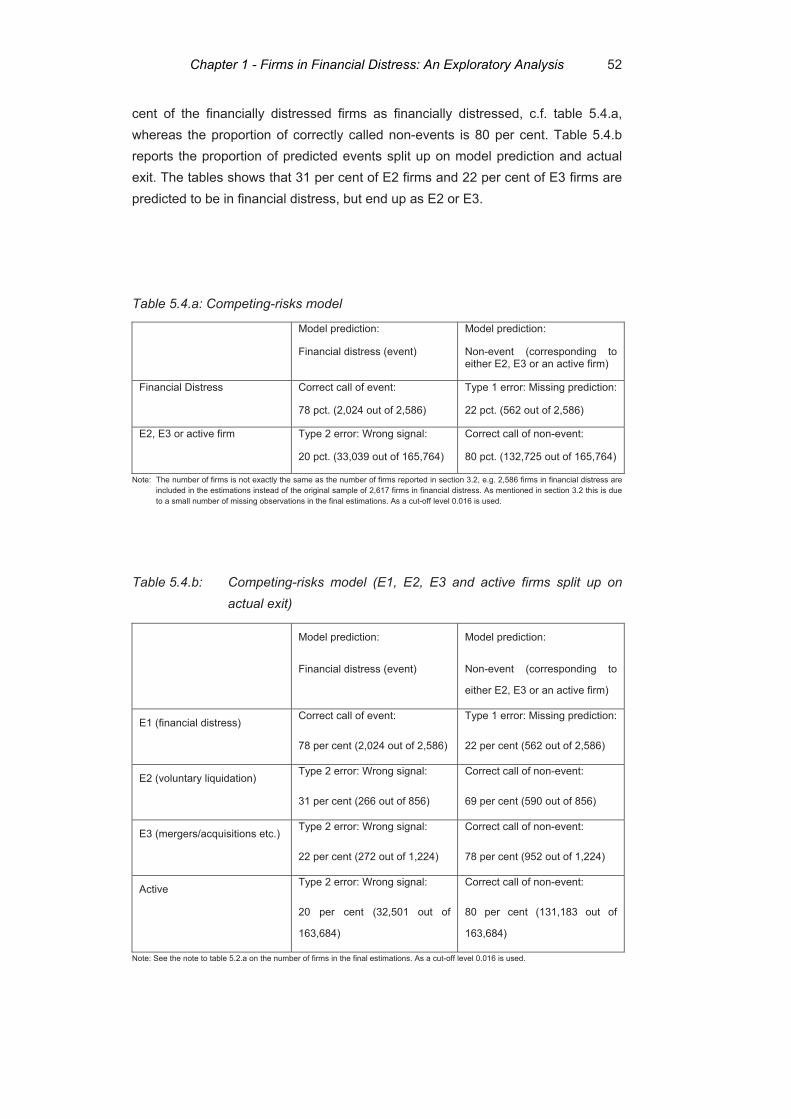
52

cent of the financially distressed firms as financially distressed, c.f. table 5.4.a, whereas the proportion of correctly called non-events is 80 per cent. Table 5.4.b reports the proportion of predicted events split up on model prediction and actual exit. The tables shows that 31 per cent of E2 firms and 22 per cent of E3 firms are predicted to be in financial distress, but end up as E2 or E3.

Table 5.4.a: Competing-risks model

Model prediction:

Financial distress (event)

Model prediction:

Non-event (corresponding to either E2, E3 or an active firm)

Financial Distress Correct call of event:

78 pct. (2,024 out of 2,586)

Type 1 error: Missing prediction:

22 pct. (562 out of 2,586)

E2, E3 or active firm Type 2 error: Wrong signal:

20 pct. (33,039 out of 165,764)

Correct call of non-event:

80 pct. (132,725 out of 165,764)

Note: The number of firms is not exactly the same as the number of firms reported in section 3.2, e.g. 2,586 firms in financial distress are included in the estimations instead of the original sample of 2,617 firms in financial distress. As mentioned in section 3.2 this is due to a small number of missing observations in the final estimations. As a cut-off level 0.016 is used.

Table 5.4.b: Competing-risks model (E1, E2, E3 and active firms split up on actual exit)

Model prediction:


Model prediction:

Non-event (corresponding to

either E2, E3 or an active firm)

E1 (financial distress) Correct call of event:

78 per cent (2,024 out of 2,586)


22 per cent (562 out of 2,586)

E2 (voluntary liquidation) Type 2 error: Wrong signal:

31 per cent (266 out of 856)



E3 (mergers/acquisitions etc.) Type 2 error: Wrong signal:




Active Type 2 error: Wrong signal:

20 per cent (32,501 out of

163,684)



163,684)

Note: See the note to table 5.2.a on the number of firms in the final estimations. As a cut-off level 0.016 is used.


53

In figure 5.4.a the predicted value of the firms that are predicted to end up in financial distress (i.e. have a predicted value above 0.016) are sketched. The predictions are split up on the actual exit. This means that what can be read from the table is the actual exit of the firms that are predicted to end up in financial distress. This is important. According to the model the firms are predicted to end up as financially distressed. But because the actual exit is known, the firms that are predicted as financially distressed can be grouped according to the actual exit. The predictions are split up on chosen percentiles (1, 10, 25, 50, 75, 90 and 99 per cent). Take one of them, e.g. the 90th percentile. As is the expectation, the figure shows that at the 90th percentile, firms that actually end up in financial distress have a higher predicted value than firms that actually end up as E2, E3 or active firms. The more interesting thing to note is that firms that end up exiting for E2 or E3 reasons (but are predicted to enter financial distress) have higher predicted values than the firms that end up as active firms (but are predicted to enter financial distress).

Figure 5.4.a: Firms predicted as financially distressed in the competing-risks model: The distribution of predictions split up on E1, E2, E3 and active firms

0

0.1

0.2

0.3

0.4

0.5

0.6

0.7

0.8

0.9

1% 10% 25% 50% 75% 90% 99%

Percentile

Pred

ictio

n

E1 E2 E3 Active


54

Figure 5.4.b: Firms predicted as non-events in the competing-risks model (E2, E3 and active): The distribution of predictions split up on E1, E2, E3 and active firms

0

0.002

0.004

0.006

0.008

0.01

0.012

0.014

0.016

0.018

1% 10% 25% 50% 75% 90% 99%

Percentile

Pred

ictio

n

E1 E2 E3 Active

To conclude, figure 5.4.a shows that the firms that actually end up as E2 and E3 firms have predicted values that are higher than the predicted values of the firms that end up as active firms, or in other words, compared to the active firms that are predicted to end up in financial distress (the so called worst faring active firms), the E2 and E3 firms that are predicted to end up in financial distress (the so called worst faring E2 and E3 firms) have predicted values that are closer to the predictions that the E1 firms generate.

Figure 5.4.b shows the predicted value of the firms that are predicted to end up as non-events (i.e. have a predicted value below 0.016). The predictions are split up on the actual exit. Again this means that what can be read from the figure is the actual exit of the firms that are predicted to end up as non-events. The figure shows that the firms that actually end up as E2 or E3 firms have predicted values that are smaller than the predicted values of the firms that actually end up as active firms. Compared to E2 and E3 firms, active firms have predicted values that are closer to the predictions that the E1 firms generate (This is the case for all the chosen percentiles in figure 5.4.b, except for the 99 percentile for the E3 firms).

The overall conclusion from figures 5.4.a and 5.4.b is that it seems as if the worst faring E2 and E3 firms (the ones that are predicted to enter financial distress, c.f. figures 5.4.a) are “weaker” than the worst faring active firms (although it is not so much), and that the best faring E2 and E3 firms (the ones that are predicted to be


55

active, c.f. figure 5.4.b) are “stronger” than the best faring active firms (although it is not so much).

The cut-off level should depend on the “agents” objective function, i.e. the objective function of the policy maker or the credit institutions etc. that uses the model. If the cost of not predicting more events is high, one can reduce the cut-off level used in table 5.4.a in order to predict more events. This will be at the cost of an increased number of type 2 errors (wrong signal). A reduction in the cut-off level to 0.008 increases the proportion of correctly called events to 91 per cent and the proportion of type 2 errors to 42 per cent. If one judges, that the cost of making too many type 2 errors is high, one can increase the cut-off level in order to make less type 2 errors. This will be at the cost of less correctly called events. If one increases the cut-off level to 0.04, the proportion of type 2 errors reduces to 6 per cent and the proportion of correctly called events is reduced to 50 per cent.

6. A Comparison with a Simple Financial Distress Model In the above sections a parametric competing-risks model is set up. In section 6.2 the estimated parameters and the predictive ability of that model is compared to a simple financial distress model, which is estimated as a hazard model, where the firms that exit for other reasons than financial distress are treated as censored or no longer observed, when they leave the sample. This simple financial distress model follows the model set up in Shumway (2001). It is called the E1event model. The model set ups (parameter estimates and predictive ability) are compared despite the fact that the test for the pooling of states showed that E2, E3 and active firms should not be pooled. In this context, as an aside, note that if one were to follow the argument in Hillegeist, Keating, Cram and Lundstedt (2004) here, one would not have compared the models predictive ability. Hillegeist et al. (2004:18f) argue that they only use statistical tests to compare model performance as “it allows us to determine whether differences in performance are statistically significant. Such determinations are not possible using prediction-oriented tests.” 18

An important difference between the E1event model and the competing-risks model is that the E1event model does not deliver the parameter estimates on the E2 and E3 hazard, but there are also other differences, c.f. section 6.1. In section 6.1 an example shows that an important distinction between the E1event model and the competing-risks model is that in the multinomial logit model, if a variable x has a positive coefficient, an increase in the variable may lead to an increase in the probability of exiting as an E1 firm, but it need not be the case, as the probability of another outcome may increase by even more. This is not the case in the E1event

18 As Hillegeist et al. (2004) have set up non-nested models they use the Vuong-test to compare the

models. The specification test used in this paper is the test for the pooling of states in the multinomial logit model, c.f. Cramer and Ridder (1991). It would have been interesting to see how much the predictive abilities of their models differ.


56

model, where, if a variable x has a positive coefficient, one knows, that every increase in x results in an increase in the probability of the designated outcome. The interpretational differences in the two model set ups are pointed out in textbooks (see e.g. Greene (2003), Wooldridge (2002) and Jenkins (2003)), but, as they are often not appropriately appreciated in applied work, they are considered important enough to be re-iterated here in this section, where the competing-risks model is compared to a simple financial distress model. The section is inspired by Allison (2001).

6.1. Interpretational Differences in the Competing-risks Model and the Simple Financial Distress Model

This section presents an example, which shows an extra benefit of estimating the model as a competing-risks model instead of a simple financial distress model. It shows that in the competing-risks model, if a variable x has a positive coefficient, an increase in the variable may lead to an increase in the probability of exiting as an E1, but it need not be the case, as the probability of another outcome may increase by even more. This is not the case in the E1event model.

The estimations of the E1event model deliver:

tEE

E

activeEE

E Xp

ph

h1

1

1

32

1 ')1

log()log( β=−

=++

⇔

)'exp(11

)'exp(1)'exp(

11

111

tEtE

tEEE XX

Xph

βββ

−+=

+==

If there is only a single explanatory variable in the model (x), i.e. short term debt to total assets, and if we have that the intercept is equal to e.g. 0 and 1=β , then the equation can be graphed to produce the curve, which is depicted in figure 6.1.a.

From the figure it is seen, that as x gets large, the probability of moving into financial distress is close to 1, and when x is small, the probability of moving into financial distress is close to 0. The effect of a unit change in x depends on where one starts on the curve. When the probability of moving into financial distress is near 0.5, then the effect is large. When the probability of moving into financial distress is close to 0 or 1, the effect is small.

The slope of the curve is given by

)1( 111

EEE ppx

p−=

∂∂ β .

When 1=β and the probability of moving into financial distress is 0.5, then a 1-unit increase in x produces an increase in the probability of 0.25.


57

Figure 6.1.a: Graph of the E1event model for a single explanatory variable (probability of E1)

0

0.1

0.2

0.3

0.4

0.5

0.6

0.7

0.8

0.9

1

-4 -3 -2 -1 0 1 2 3 4The explanatory variable (X)

Prob

abili

ty

In the E1event model, if a variable x has a positive coefficient, one knows that every increase in x results in an increase in the probability of the designated outcome. This is not always true in the multinomial logit model. Consider the following hypothetical example. Suppose that the dependent variable has three categories (E1, E2 and active firms) and there is a single independent variable x, and that when the multinomial logit model is estimated, the following equations are obtained:

xpp

hh

active

E

active

E 0.10.1)log()log( 11 −==

xpp

hh

active

E

active

E 0.20.1)log()log( 22 −==

In the hypothetical example we assume that intercepts of both hazards are equal to

1 and furthermore that the estimated coefficient is -1 for the E1 hazard and -2 for

the E2 hazard.

The above equations can be solved for 1Ep . The following equation is then obtained

xx

x

E eeep 211

1

1 1 −−

−

++=

A graph of this equation is shown in figure 6.1.b.

In a binomial setting with only E1 firms and active firms, the interpretation of


58

xpp

hh

active

E

active

E 0.10.1)log()log( 11 −== is, that an increase in x would decrease

the likelihood of an E1 exit. In the multinomial logit setting, where both exit possibilities need to be taken into account, the E1 and the E2 exit, an increase in x does not always decrease the likelihood of an E1 exit. Figure 6.1.b shows that when the explanatory variable is below 0.5, an increase in x produce increases in the probability of E1, whereas, when the explanatory variable is above 0.5, an increase in x produce decreases in the probability of E1. The reason for this effect is that increases in x move firms in the E1 category to the active category, but that increases in x also move firms in the E2 category to the E1 category. For a low level of the explanatory variable most cases are in the E2 category, and therefore most of the movement is from the E2 category to the E1 category and so the proportion of E1 firms goes up. In the end, only a few firms in the E2 category are left and so the movement is from the E1 category to the active category, and therefore, the proportion of E1 firms declines.

Figure 6.1.b: Graph of the probability of an E1 event in the multinomial logit model

0

0,05

0,1

0,15

0,2

0,25

0,3

0,35

0,4

0,45

0,5

-4 -3 -2 -1 0 1 2 3 4

The explanatory variable (X)

Prob

abili

ty o

f E1


59

Figure 6.1.c: Graph of the probability of an E2 event in the multinomial logit model

0

0,2

0,4

0,6

0,8

1

1,2

-4 -3 -2 -1 0 1 2 3 4

The explanatory variable (X)

The

prob

abili

ty o

f E2

In figure 6.1.c the probability of an E2 event in the multionomial logit model is sketched. The graph is based on the following equation:

xx

x

E eeep 211

21

2 1 −−

−

++=

For the chosen parameters it is seen, that an increase in the explanatory variable always leads to a decrease in the probability of being an E2 firm.

To conclude, the important thing to notice in the multinomial model is that it allows that an increase in a variable with a positive (negative) coefficient in the equation for one outcome need not lead to an increase (decrease) in the probability of that outcome. This is not the case in the E1event model, where, if a variable x has a positive (negative) coefficient, one knows, that every increase in x results in an increase (decrease) in the probability of the designated outcome.

The implication of this for credit-scoring models is that once the model is estimated as a competing-risks model, it can be used to assess the effect on a possible increase or decrease in one or more explanatory variables (i.e. as a stress-testing tool).


60

6.2. Parameter Estimates and the Proportion of Correct Predictions The results obtained in the multinomial logit model (the estimated parameters and the predictive ability) are compared to the E1event model.

When comparing the sign of the parameter estimates of the financial distress hazard in the competing-risks model and the parameter estimates in the E1event model, it is seen that all parameter estimates have the same sign, but that the magnitude differs, although it is not so much, c.f. the appendix on figures and tables (section 10).

Table 6.2.a: E1event model

Model prediction:

Event (=an event)

Model prediction:

Non-event (=active firms)

Event (=an exit) Correct call of event:

78 pct. (2,026 out of 2,586)


22 pct. (560 out of 2,586)

Non-event (=active firms) Type 2 error: Wrong signal:

20 pct. (33,140 out of 165,764)


80 pct. (132,624 out of 165,764)

Note: The proportion of events to non-events is 0.016, and therefore 0.016 is used as the cut-off level. See also the note attached to table 5.4.a. concerning missing data in the final estimations.

Table 6.2.b: E1event model (E1, E2, E3 and active firms split up on actual exit)

Model prediction:


Model prediction:

Non-event (corresponding to

either E2, E3 or an active firm)


78 per cent (2,026 out of 2,586)







E3 (mergers/acquisitions etc.) Type 2 error: Wrong signal:




Active Type 2 error: Wrong signal:


163,684)



163,684)

Note: See the note to table 5.4.a on the number of firms in the final estimations. As a cut-off level 0.016 is used.


61

Figure 6.2.c: The 100 observations with the highest prediction in the competing-risks model and the E1event model

0.65

0.7

0.75

0.8

0.85

0.9

0.95

1

1 4 7 10 13 16 19 22 25 28 31 34 37 40 43 46 49 52 55 58 61 64 67 70 73 76 79 82 85 88 91 94 97

Number of observations

Pred

icte

d va

lue

Comp.risks E1event model

The competing-risks model and the E1event model generate predictions that are very similar, c.f. tables 6.2.a, 6.2.b, 5.4.a and 5.4.b. The tables show that the E1event model correctly classifies 132,624 non-events and 2,026 events, whereas the competing-risks model correctly classifies 132,725 non-events and 2,024 events. Furthermore it is seen, that the number of correctly classified E2 firms is 590 in the competing-risks specification and 579 in the E1event model, and that the number of correctly classified E3 firms is 952 in the competing-risks specification and 946 in the E1event model.

In figure 6.2.c the 100 observations with the highest predicted value in the competing-risks model and the E1event model are sketched. The figure suggests that the predictions are alike in the two specifications, i.e. the same conclusion as above. The conclusion is not changed when looking at the whole distribution of the predictions in the two model specifications, c.f. the appendix on predictions (section 11).

That the two models are equally good at predicting non-events and events is puzzling. The specification test on pooling states in the multinomial logit model showed, c.f. section 5.1, that the firms that end up exiting for E2 and E3 reasons are significantly different from the active firms, thereby indicating that the pooling of states does not give the correct specification. The way to interpret the result from


62

the test of pooling of states and the comparison of predictive abilities of the two model set ups is that the correct specification does not allow for the pooling of states, but that it seems as the biases arising from it are relatively small (in this setting).

7. Conclusion This paper sets up a model that can predict the firms that end up in financial distress. As the firms in the non-financial sector can exit for various reasons (financial distress, voluntary liquidation and because they are merged or acquired etc.) the method of competing-risks models seems appropriate. Following Allison (1982) independent exits and a special kind of destination-specific hazard rates are assumed, and a parametric discrete competing-risks model is estimated as a multinomial logit model. The model is estimated using a panel data set containing information on the whole population of Danish non-financial public limited liability companies and private limited liability companies that existed between 1995 and 2001, covering around 30,000 firms and more than 150,000 firm-year observations. More than 20 explanatory variables are included in the estimations, and all sectors of the Danish economy are covered.

As the competing-risks model is estimated as a multinomial logit model, two specification tests for multinomial logit models are presented and performed. The first is the test for the independence of irrelevant alternatives (IIA assumption). The second is a test for pooling states in the multinomial logit model. The tests show that the competing-risks model should be specified as a multinomial logit model in which all states are included (neither E2 or E3 exits should be left out according to the IIA test) and where E2 and E3 exits are treated as separate exits (and not lumped together with active firms. This is the result from the pooling of states).

The parameter estimates, which are obtained when the competing-risks model is estimated, are presented. All variables for which a sign was expected have the expected sign. The core and proxy variables, which were expected and estimated to have a negative coefficient, are age, size, the return on net assets, the solvency ratio, the diversification variables and the wholly-owned subsidiary dummy. A negative sign indicates that the higher these variables are the less likely a firm is to enter financial distress (relative to staying active). In this respect note that the duration dependence is estimated to be almost linear and downward-sloping until the firms reach the age of 15, and from the age of 15 the effect is approximately constant. The variables short term debt to total assets, the private limited liability dummy and the dummy for having critical comments from the auditors were expected and estimated to have a positive sign, indicating that the higher these variables are, the more likely a firm is to enter financial distress, relative to staying active.


63

For some variables a specific sign is not expected. This was the case for the proxy variables ultimate parent company, owned by a fund, owned by the public sector, local authority group 2, 3, 4 and 5, and the control variable primary bank group 1, group 2, and group 3 & 4. The sign of the parameter of the dummy variable ultimate parent company is positive, and so the odds, that an ultimate parent company will enter financial distress relative to staying active compared to companies that are not ultimate parent companies, are higher, indicating that ultimate parent companies have a tendency to let the not-so-well-performing subsidiaries drain resources from the group as a whole, including the ultimate parent company, e.g. because of reputational risk. The effects of fund ownership and public sector ownership are not significant. All local authority groups, except of local authority group 4, which measures the effect of being situated outside Zealand in other local authorities with 50,000 inhabitants or more, relative to being situated in Copenhagen and Frederiksberg, have smaller odds of moving into financial distress compared to the companies situated in Copenhagen and Frederiksberg (group 1). This means that firms that are situated in local authorities in the county of Copenhagen (group 2), local authorities in the county of Frederiksborg and Roskilde (group 3) and local authorities with less than 50,000 inhabitants are less likely to enter financial distress, relative to active firms. The odds that firms that register a group 2 bank (defined as banks with a working capital from kr. 3 billion up to kr. 25 billion), as their primary bank enter financial distress are higher than the odds for firms that do not register a bank connection. There is no difference between not registering a bank at all and registering a group 1 or group 3 & 4 banks (defined as banks that have a working capital of kr. 25 billion and above (group 1) and banks that have a working capital up to kr. 3 billion (group 3 & 4).

The dummy variables that control for the sector affiliation in the competing-risks model show that compared to being a manufacturing firm (reference dummy) the odds that the firms that belong to one of the following sectors move into financial distress are smaller: trade and hotel, transport, business service, public service activities, and organizations, etc. On the contrary, the odds that the firms that have the sector affiliation "unknown” move into financial distress are higher. Firms with the other sector affiliations are not significantly different from firms in the manufacturing sector. All firms that are in the self-constructed IT- and telecommunication category have higher odds of moving into financial distress than all other firms.

The section on goodness-of-fit illustrates that the competing-risks model can distinguish between the various exits, and the section on the predictive ability of the model shows, that the model correctly classifies 78 per cent of the financially distressed firms as financially distressed, whereas the proportion of correctly called non-events is 80 per cent (when a cut-off level of the proportion of financially


64

distressed firms used in the estimations, corresponding to 0.016, is used). The model is evaluated in-time and in-sample, as it was chosen to use all the available data in the estimations to have as long a time series as possible. The real test of the model’s predictive ability will of course be the practical confrontation with data for recent periods as it emerges. Ideally, the model should be evaluated both out-of-time and out-of-sample.

Further investigations of the predictions of the model show, that the firms that are predicted to end up as financially distressed, but actually end up as E2 and E3 firms, have predicted values that are higher than the predicted values of the firms that end up as active firms. Or, in other words, compared to the active firms that are predicted to end up in financial distress (the so called worst faring active firms), the E2 and E3 firms that are predicted to end up in financial distress (the so called worst faring E2 and E3 firms) have predicted values that are closer to the predictions that the E1 firms generate. Also, when looking at the firms that actually end up as E2 or E3 firms, but are predicted to be non-events, it is seen, that they have predicted values that are smaller than the predicted values of the firms that actually end up as active firms. Compared to E2 and E3 firms, active firms have predicted values that are closer to the predictions that the E1 firms generate (This is the case for all the chose percentiles, except for the 99 percentile for the E3 firms). The overall conclusion of these findings are, that it seems as if the worst faring E2 and E3 firms (the ones that are predicted to enter financial distress) are “weaker” than the worst faring active firms, and that the best faring E2 and E3 firms are “stronger” than the best faring active firms.

The competing-risks model is compared to a simple financial distress model, which is estimated as a hazard model, where the firms that exit for other reasons than financial distress are treated as censored or no longer observed, when they leave the sample. A comparison of the competing-risks E1 parameter estimates with the parameter estimates in the E1event model shows that the sign of the significant parameters are the same in the two model specifications, only the magnitude of the parameter estimates differ to some extent. Furthermore, the comparison shows that the models generate predictions that are very similar. This is puzzling as one would think that the competing-risk model would do a better job. The specification test on the pooling of states in the multinomial logit model shows, that the competing-risks model should be specified as a multinomial logit model where E2 and E3 exits are treated as separate exits (and not lumped together with active firms). The way to interpret the result from the test of pooling and states and the comparison of predictive abilities of the two model set ups is that the correct specification does not allow for the pooling of states, but that it seems as the biases arising from it are relatively small (in this setting).

An important distinction between the E1event model and the competing-risks model is that the multinomial model allows that if a variable x has a positive


65

coefficient, an increase in the variable may lead to an increase in the probability of exiting as an E2 firm (say this is the outcome we are interested in), but it need not be the case, as the probability of another outcome may increase by even more. This is not the case in the E1event model, where, if a variable x has a positive coefficient, one knows, that every increase in x results in an increase in the probability of the designated outcome.


66

8. LITERATURE D’Addio, A. and M. Rosholm, 2002. Left-Censoring in Duration Data: Theory and Applications. Working Paper No. 2002-5, Department of Economics, School of Economics and Management, University of Aarhus

Agarwal, R. and D. B. Audretsch, 2001. Does Entry Size Matter? The Impact of the Life Cycle and Technology on Firm Survival. The Journal of Industrial Economics, vol. XLIX, no. 1, pp. 21-43

Allison, P. D., 1982. Discrete-time Methods for the Analysis of Event Histories. In Samuel Leinhardt (ed.), Sociological Methodology 1982, San Francisco: Jossey-Bass, pp. 61-98

Allison, P. D., 2001. Logistic Regression using the SAS System. Theory and Application. Cary, NC, USA: SAS Institute

Altman, E. I., 1968. Financial Ratios, Discriminant Analysis and the Prediction of Corporate Bankruptcy. Journal of Finance, vol. 23, no. 4, pp. 589-609

Altman, E. I. and A. Saunders, 1998. Credit risk measurement: Developments over the last 20 years. Journal of Banking and Finance, vol. 21, pp. 1721-1742

Arellano, M., 2003. Panel Data Econometrics. Advanced Texts in Econometrics. New York, USA: Oxford University Press

Audretsch, D. B., 1991. New-Firm Survival and the Technological Regime. The Review of Economics and Statistics, vol. 73, no. 3, pp 441- 450

Audretch, D. B. and T. Mahmood, 1995. New Firm Survival: new Results using a Hazard Function. The Review of Economic and Statistics, vol. 77, no. 1, pp. 97-103

Balcaen, S. and H. Ooghe, 2004. Alternative methodologies in studies on business failure: do they produce better results than the classical statistical methods? Working Paper 2004/249, Faculteit Economie en Bedrijfskunde

Bardos, M., 1998. Detecting the risk of company failure at the Banque de France. Journal of Banking & Finance, vol. 22, pp. 1405-1419

Bardos, M., 2001. Recent developments in the Banque de France’s scoring method. Banque de France Bulletin Digest, no. 93, September 2001

Basel Committee on Banking Supervision, 2004. International Convergence of Capital Measurement and Capital Standards. A Revised Framework. Bank for International Settlements, June 2004

Bates, T., 1990. Entrepreneur Human Capital Inputs and Small Business Longevity. The Review of Economics and Statistics, vol. 72, no. 4, pp. 551-559


67

Beaver, W., 1966. Financial Ratios as Predictors of Bankruptcy. Journal of Accounting Research, vol. 6, pp. 71-102

Beaver, W., 1968. Market Prices, Financial Ratios, and the Prediction of Failure. Journal of Accounting Research, vol. 8, pp. 179-92

Begg, C. B. and R. Gray, 1984. Calculation of polychotomous logistic regression parameters using individualized regressions. Biometrika, 71, 1, pp. 11-18

Berger, P. G. and W. Ofek, 1995. Diversification's Effect on Firm Value. Journal of Financial Economics, vol. 7, pp. 39-65

Bernhardsen, E., 2001. A Model of Bankruptcy Prediction. Norges Bank Working Paper, ANO 2001/10

Bhattacharjee, A., C. Higson, S. Holly and P. Kattuman, 2004. Business Failure in UK and US Quoted Firms: Impact of Macroeconomic Instability and the Role of Legal Institutions. Unpublished manuscript, January 2004.

Borup, L., Kurek, D. and A. D. Rommer, 2005. Assessing the consequences of Basel II: Are there incentives for cherry-picking when banks pool data across countries? Working Paper no. 27, Danmarks Nationalbank

Brito, P. and A. S. Mello, 1995. Financial Constraints and Firm Post-entry Performance. International Journal of Industrial Organisation, vol. 13, pp. 543-565

Bunn, P. and V. Redwood, 2003. Company-accounts-based modelling of business failure and the implications for financial stability. Working paper no. 210, Bank of England

Bunn, P., 2003. Company-accounts-based Modelling of Business Failure. Financial Stability Review: December 2003, Bank of England

Cramer, J. S. and G. Ridder, 1991. Pooling states in the multinomial logit model. Journal of Econometrics, 47, pp. 267-272

Danmarks Nationalbank, 2003. Danish Government Borrowing and Debt 2003. Copenhagen, Denmark: Danmarks Nationalbank

Danmarks Nationalbank, 2005. Financial Stability 2005. Copenhagen, Denmark: Danmarks Nationalbank

Dimitras, A. I., Zanakis, S. H. and C. Zopounidis, 1996. A survey of business failures with an emphasis on prediction methods and industrial applications. European Journal of Operational Research, vol. 90, pp. 487-513

Elizalde, A. and R. Repullo, 2004. Economic and regulatory capital. What is the difference? CEMFI Working Paper 0422, December 2004


68

Ericson, R. and A. Pakes, 1995. Markov-Perfect Industry Dynamics: A Framework for Empirical Work. Review of Economic Studies, vol. 62, pp. 53-82

European Central Bank, 2005. Financial Stability Review, June 2005. European Central Bank

Fahrmeir, L. and S. Wagenpfeil, 1996. Smoothing Hazard Functions and Time-Varying Effects in Discrete Duration and Competing Risks Models. Journal of the American Statistical Association, 91, pp. 1584-1594

Fotopoulos, G. and H. Louri, 2000. Location and Survival of New Entry. Small Business Economics, vol. 14, pp. 311-321

Frame, W. S., A. Srinivasan and L. Woosley, 2001. The Effect of Credit Scoring on Small-business Lending. Journal of Money, Credit and Banking, vol. 33, no. 3, pp. 813 - 825

Franses, P. H. and R. Paap, 2001. Quantitative Models in Marketing Research. Cambridge University Press

Gort, M. and S. Klepper, 1982. Time Paths in the Diffusion of Product Innovations. The Economic Journal, vol. 92, no. 367, pp. 630-653

Greene, W., 2003. Econometric Analysis. New Jersey, USA: Prentice Hall

Grunert, J., Norden, L. and M. Weber, 2005. The role of non-financial factors in internal credit ratings. Journal of Banking and Finance, vol. 29, pp. 509-531

Harhoff, D., K. Stahl and M. Woywode, 1998. Legal Form, Growth and Exit of West German Firms: Empirical Results for Manufacturing, Trade and Service Industries. Journal of Industrial Economics, vol. 46, pp. 453-488

Henley, A., 1998. Residential mobility, housing equity and the labour market. The Economic Journal, 108, pp. 414-427

Henneke, J. and S. Trück, 2005. Capital requirements for SMEs under the Revised Basel II Framework. Unpublished Manuscript

Hillegeist, S. A., Keating, E. K., Cram, D. P. and K. G. Lundstedt, 2004. Assessing the Probability of Bankruptcy. Review of Accounting Studies, no. 9, pp. 5-34

Jenkins, S., 1995. Easy Estimation Methods for Discrete-Time Duration Models. Oxford Bulletin of Economics and Statistics, vol. 57, no. 1, pp. 129-138

Jenkins, S., 2003. Survival Analysis. Unpublished manuscript

Jones, F. L., 1987. Current Techniques in Bankruptcy Prediction. Journal of Accounting Literature, vol. 6, pp. 131-164


69

Jones, S. and D. A. Hensher, 2004. Predicting Firm Financial Distress: A Mixed Logit Model. The Accounting Review, vol. 79, no. 4, pp. 1011-1038

Jovanovic, B., 1982. Selection and the Evolution of Industry. Econometrica, vol. 50, no. 3, pp. 649-670

Jovanovic, B., 1993. The Diversification of Production. Brookings Papers on economic activity: Microeconomics, vol. 1, pp. 197-247

Jovanovic, B. and G. MacDonald, 1994. The Life Cycle of a Competitive Industry. Journal of Political Economy, vol. 102, no. 2, pp. 322-347

Kaiser, U., 2001. Moving in and out of Financial Distress: Evidence for Newly Founded Service Sector Firms. Unpublished manuscript

Klepper, S., 1996. Entry, Exit, Growth and Innovation over the Product Life Cycle. American Economic Review, vol. 86, no. 3, pp. 562-583

Konkurrencestyrelsen, 2003. Konkurrenceredegørelse 2003. Copenhagen, Denmark: The Danish Competition Authority

Köke, J., 2001. Determinants of acquisition and failure: Stylized facts and lessons for empirical studies. Discussion Paper No. 01-30, ZEW

Lamont, O. A. and C. Polk, 2002. Does Diversification Destroy Value? Evidence from the Industry Shocks. Journal of Financial Economics, vol. 63, pp. 51-77

Lando, D., 2004. Credit Risk Modeling. Theory and Applications. Princeton Series in Finance

Lau, A. H.-L., 1987. A Five-State Financial Distress Prediction Model. Journal of Accounting Research, vol. 25, no. 1, pp. 127-138

Lykke, M., Pedersen K. J. and H. M. Vinther, 2004. A Failure-Rate Model for the Danish Corporate Sector. Danmarks Nationalbank Working Paper, no. 16

Malchow-Møller, N. and M. Svarer, 2002. Estimation of the Multinomial Logit Model with Random Effects. Discussion Paper No 2002-16. Accepted for publication in Applied Economic Letters

Møller, M., N. C. Nielsen and J. Ø. Poulsen, 1998. Hvem bærer kreditrisikoen på danske virksomheder? Nationaløkonomisk Tidsskrift, vol. 136, pp. 315-332.

Ohlson, J. A., 1980. Financial Ratios and the Probabilistic Prediction of Bankruptcy. Journal of Accounting Research, vol. 19, pp. 109-131

Pakes, A. and R. Ericsson, 1998. Empirical Implications of alternative Models of Firm Dynamics. Journal of Economic Theory, vol. 79, pp. 1-45


70

Pedersen, K. J., 2002. Regnskabsbaseret konkursmodel for danske virksomheder – teori og empiri. Dissertation, University of Copenhagen

Phillips, B. D. and B. A. Kirchhoff, 1989. Formation, Growth and Survival; Small Firm Dynamics in the U.S. Economy. Small Business Economics, vol. 1, pp. 65-74

Prantl, S., 2003. Bankruptcy and Voluntary Liquidation: Evidence for New Firms in East and West Germany after Unification. Discussion Paper No. 03-72, ZEW

Rajan, R., H. Servaes and L. Zingales, 2000. The Cost of Diversity: The Diversification Discount and Inefficient Investment. The Journal of Finance, vol. LV, no. 1, pp. 35-80

Rommer, A. D., 2005 (a). A Comparative Analysis of the Determinants of Financial Distress in French, Italian and Spanish firms. Working Paper no. 26, Danmarks Nationalbank

Rommer, A. D., 2005 (b). Testing the Assumptions of Credit-scoring Models. Working Paper no. 28, Danmarks Nationalbank

Røjkjær, C. and H. Klinker, 1994. Model til konkursforudsigelse i Danmark. Finans/invest, 1/94, pp. 18-22

Schary, M. A., 1991. The probability of exit. RAND Journal of Economics, vol. 22, no. 3, pp. 339-353

Statistics Denmark, 2001. Nye virksomheders overlevelse 1994-1998. NYT fra Danmarks Statistik nr. 178

Stiglitz, J. E. and A. Weiss, 1981. Credit Rationing in Markets with Imperfect Information. The American Economic Review, vol. 71, no. 3, pp. 393-421

Shumway, T., 2001. Forecasting Bankruptcy More Accurately: A Simple Hazard Model. Journal of Business, vol. 74, no. 1, pp. 101-124

Tirole, J., 1997. The Theory of Industrial Organization. Cambridge (Mass.), USA: The MIT Press

Train, K., 2003. Discrete Choice Methods with Simulation. New York, USA: Cambridge University Press

Wooldridge, J. M., 2002. Econometric Analysis of Cross section and Panel data. Cambridge (Mass.), USA: The MIT Press

Wooldridge, J. M., 2003. Introductory Econometrics. A Modern Approach. Ohio, USA: Thomson South-Western


71

9. Appendix: Data

Definitions

Return on net assets = primary operating result as a ratio of assets19

The solvency ratio = equity capital divided by total liabilities

Short term debt to total assets

Firm size = ln(total assets)

Concentration: The concentration in a specific sector is measured by the CR4-index, which is calculated as the sum of the market shares in the four largest companies as a percentage of the total domestic turnover in a specific sector. The index is based on the VAT statistics calculated by Statistics Denmark. For details on the CR4 index, see Konkurrencestyrelsen (2003:chapter 2.3).

Firm age: A dummy for every year is constructed (reference category is firms that are one year old. Firms that are 30 years old or more have the dummy 30 years old or more). Only significant dummies are included and presented in the final estimation results.

Critical comments from the auditors: If there are critical comments from the auditors, the dummy is equal to 1. The critical comments can be "illegal loans have been adopted", "financial statement is incomplete", "inconsistencies in the profit and loss account", etc. These comments indicate illegal activities or that there are discrepancies in the financial statement. Firms with the following critical comments are not included in the "critical comments from the auditors” measure, as they indicate that the firm is not viable (and they are thus likely to be correlated with the dependent variable, the E1 measure): "operation cannot be continued", "there are reservations made to the continuation of operation", etc.

Legal status: If the company is a private limited liability company, the dummy is equal to 1. (Private limited liability companies are compared to public limited liability companies).

Publicly traded company: If the company is publicly traded, the dummy is equal to 1.

19

The primary operating result in year t is divided by total assets in year t. One could also have chosen to divide by the total assets in year t-1 or to take the average of assets in year t and t-1, as it could be argued, that these figures would better reflect the actual resources available to the firm. Nonetheless, assets in year t is used since 1) otherwise, a whole cross-section of observations would be lost, 2) the companies might change the accounting principles as to some extent they can choose between different types of accounting methods, and 3) companies might have acquired new companies or sold of divisions, and therefore that it is not the same company as the year before.


72

Ownership variables are constructed: Public sector ownership: If the company is owned by the public sector, the dummy is equal to 1. Fund ownership: If the company is owned by a fund, the dummy is equal to 1.

Dummy variables indicating whether or not the specific firm is an ultimate parent company or a wholly-owned subsidiary are constructed: Ultimate parent company: If the company is an ultimate parent company, the dummy is equal to 1. Wholly-owned subsidiary: If the company is a wholly-owned subsidiary, the dummy is equal to 1.

Sector affiliation: There is a dummy for each main category according to table 9. Statistics Denmark does not have a sector affiliation category called "IT and telecommunication companies", and so an IT and telecommunication company dummy is constructed. A firm can have 9 sector affiliation codes. If one of the affiliation codes is in the IT and telecommunication sector, which is defined as manufacturing of IT software, hardware, etc., manufacturing of telephone sets, switchboards, and telex apparatus, etc., then the IT and telecommunication dummy is set to 1.

Table 9: Sector affiliation

Sector Affiliation NACE-codes 1. Farming 01 2. Forestry 02 3. Fishing 05 4. Mining 10-14 5. Manufacturing 15-37 6. Energy (“Production of electricity, manufacturing of gas,

collection, purification and distribution of water") 40-41

7. Construction (“Construction of buildings and civil engineering works, various contractors and other building completion”)

45

8. Trade and hotel (“Wholesale, retail, repair and hotels”) 50-52, 55 9. Transport 60-64 10. Business service (“Development and selling of real estate,

renting, legal activities, advertising, etc."), (except 74.15: non-financial holding companies)

70-74

11. Public service activities (“General (overall) public service activities, education, hospital activities”)

75, 80, 85

12. Organisations, etc. (“Collection and treatment of waste, activities of business and employers organisations, etc., motion picture, video, radio, television, etc., laundering for industrial or commercial clients”)

90-93

13. Not stated 98 14. Unknown* N.A.

Note: A firm can have up to 9 different sector affiliation codes. The first of these codes, the primary sector affiliation, is used to classify the firms in the various sectors. Unknown* means, that the sector affiliation is not registered in the data base. Reasons for being unknown can be various: The company can be a new company, the company can have exited before 1998 (Up to 1998, The Danish Business Information Bureau deleted the sector affiliation when firms exited the data base)


73

Diversification: Diversification in 2 sectors (related business): If the company is operating in 2 sectors (within the same main sector), the dummy is equal to 1. Diversification in 3-9 sectors (related business): If the company is operating in 3 – 9 sectors (within the same main sector), the dummy is equal to 1. Diversification in 2 sectors (unrelated business): If the company is operating in 2 sectors (not in the same main sector), the dummy is equal to 1. Diversification in 3-9 sectors (unrelated business): If the company is operating in 3 – 9 sectors (and at least 2 are not in the same main sector), the dummy is equal to 1.

Macroeconomic environment: Controls for the macroeconomic environment are put in (a dummy for every year).

Bank: As a first go on the problem the model was estimated with a dummy equal to 1 if the company has registered a primary bank connection. Otherwise it was zero. The variable was not significant in the estimations. Then the idea was to divide the banks according to the volume of working capital. This would follow the way the Danish Financial Supervisory Authority (FSA) divides the Danish banking sector. The Danish FSA works with the following groups: Banking institutions in category 1 have a working capital of kr. 25 billion and above. Banking institutions in category 2 have a working capital from kr. 3 billion up to kr. 25 billion. Banking institutions in category 3 have a working capital from kr. 250 million up to kr. 3 billion. Banking institutions in category 4 have a working capital of less than kr. 250 million. New estimations were conducted, with the reference dummy being firms that do not register a primary bank connection at all. Compared to firms that do not register a primary bank connection, it was estimated whether or not there was on effect of registering a bank in the Danish FSA’s category 1, 2, 3 or 4.

Location: Based on the postal codes, the firms are divided into four groups depending on the location of the firms and the number of inhabitants in the local authorities that the firms belong to. Group 1, 2, 3 and 4 consist of local authorities with 50,000 inhabitants or more, and group 5 consists of local authorities with 50,000 inhabitants or less.20 Based on these groups, four dummies are constructed (the reference category is equal to group 1). Group 1: Copenhagen and Frederiksberg. Group 2: Local authorities ("kommuner") in the county of Copenhagen ("Københavns Amt") (Ballerup, Brøndby, Dragør, Gentofte, Gladsaxe, Glostrup, Herlev, Albertslund, Hvidovre, Høje-Taastrup, Ledøje-Smørum, Lyngby-Taarbæk, Rødovre, Søllerød, Ishøj, Tårnby, Vallensbæk and Værløse). Group 3: Local authorities in the county of Frederiksborg and Roskilde (Allerød, Birkerød, Farum, Fredensborg-Humlebæk, Frederikssund, Frederiksværk, Græsted-Gilleleje, Helsinge, Helsingør, Hillerød, Hundested, Hørsholm, Jægerspris, Karlebo, Skibby,

20

In the database the postal code of the firms is included. As the postal codes do not follow the local authorities in all cases, the postal codes have been attached to the local authority which has the largest part of the inhabitants in the postal code area.


74

Skævinge, Slangerup, Stenløse, Ølstykke, Bramsnæs, Greve, Gundsø, Hvalsø, Køge, Lejre, Ramsø, Roskilde, Skovbo, Solrød and Vallø). Group 4: Other local authorities with 50,000 inhabitants or more ("i største bymæssig bebyggelse") (Odense, Esbjerg, Kolding, Randers, Århus and Ålborg). Group 5: Local authorities with less than 50,000 inhabitants.

Descriptive Statistics

Solvency ratio

Number of

firms

Number Average St.dev. Max Median Min

E1 2586 0.008075 0.315697 1 0.03895 -0.9938

E2 856 0.510782 0.399105 1 0.5866 -0.9839

E3 1224 0.295536 0.278928 1 0.2659 -0.7865

Active 163684 0.296174 0.236163 1 0.267 -1

Short term debt to total assets

Number of

firms


E1 2586 0.82202 0.347881 1.9933 0.81475 0

E2 856 0.435811 0.380759 1.9839 0.33605 0

E3 1224 0.57978 0.290284 1.7865 0.5811 0

Active 163684 0.54654 0.248504 2.1882 0.5371 0


75

Return on net assets

Number of

firms


E1 2586 -0.10053 0.332614 2.4962 -0.0317 -2.9

E2 856 -0.04946 0.428661 2.7472 -0.00735 -2.9806

E3 1224 0.062423 0.217802 1.2439 0.05695 -2.0085

Active 163684 0.084787 0.164132 2.9287 0.0801 -2.9535

Size measured as ln(assets)

Number of

firms


E1 2586 8.207602 1.278804 14.386 8.11 2.996

E2 856 7.708614 1.473337 13.579 7.683 4.22

E3 1224 9.825529 1.610659 15.801 9.746 5.347

Active 163684 8.924396 1.37991 18.078 8.74 3.178

Age

Number of

firms


E1 2586 12.56342 13.15399 209 8 1

E2 856 16.36449 13.6881 142 12 1

E3 1224 22.48366 42.42949 898 15 1

Active 163684 18.70645 20.3886 897 13 1


76

Sector affiliation

Number

of firms

Farming Forestry Fishing Mining Manufac-

turing

Energy Con-

struction

E1 30 1 9 0 595 0 429

E2 4 0 4 1 106 0 107

E3 4 1 9 2 316 9 87

Active 2447 94 696 373 39276 159 26187

Number of firms

Trade etc.

Transport Busi-ness service

Public service activities

Organi-sations

Not stated

Unknown

E1 626 175 404 23 46 74 174

E2 212 40 175 19 19 46 123

E3 346 78 210 10 34 19 99

Active 52373 9530 23267 4050 2957 1472 803

Critical comments, legal status, listed companies, ultimate parents, wholly owned subsidiaries

Number of firms

Critical comments from the auditors

Legal status: Private limited companies

Listed companies

Ultimate parents

Wholly owned subsidiaries

E1 487 1532 0 49 563

E2 60 368 0 6 328

E3 15 208 0 49 909

Active 7388 65277 547 6388 46899


77

Location

Number of firms

Group 1 Group 2 Group 3 Group 4 Group 5

E1 415 333 300 423 1115

E2 155 134 102 139 326

E3 170 289 96 219 450

Active 17472 24409 18657 26497 76649

IT-dummy and primary bank

Number of firms

IT dummy Primary Bank

Cat. 1 Cat. 2 Cat. 3 Cat. 4

E1 246 6 101 149 10

E2 52 6 13 21 1

E3 106 5 25 30 0

Active 7388 442 4763 8991 202

Diversification and ownership

Number of firms

Diversification: Same Diversification: Different Ownership

2 sectors 3-9 sectors 2 sectors 3-9 sectors Public sector

Fund

E1 327 99 201 99 2 1

E2 86 16 49 15 4 5

E3 200 50 111 86 6 5

Active 31662 12016 15441 10645 262 670


78

Concentration

Sector affiliation 1995 1996 1997 1998 1999 2000 2001

1. Farming 3.0 3.0 3.2 3.6 3.8 3.3 3.9

2. Forestry 45.3 43.8 42.9 47.6 44.3 41.9 31.9

3. Fishing 4.3 5.2 5.0 5.3 6.0 8.9 7.2

4. Mining 29.1 33.0 52.4 53.8 58.8 59.2 64.9

5. Manufacturing 67.9 67.6 67.9 68.3 68.9 70.9 69.9

6. Energy 44.2 44.5 46.7 48.5 46.8 43.5 43.2

7. Construction 11.5 11.6 11.6 12.4 12.1 14.0 17.2

8. Trade & Hotel 35.3 34.6 35.2 34.2 34.2 35.2 35.8

9. Transport 56.7 57.0 57.3 58.8 60.3 61.7 62.2

10. Business service 49.1 49.2 48.2 48.7 47.7 47.9 48.6

11. Public service 5.7 4.6 3.7 3.8 3.6 3.8 5.4

12. Organisations etc. 41.7 42.2 42.0 43.3 43.9 44.3 43.9

13. Not stated1 47.1 38.7 3.2 4.0 5.2 19.1 18.6

Note : The figures in category 13 are the ones that The Danish Competition Authority has received from Statistics Denmark. As it is not possible to construct a concentration index in the sector called “unknown”, it is chosen to calculate the concentration index for this sector as an (un-weighted) average of the concentration indices in the other sectors.

Source: The Danish Competition Authority and own calculations


79

10. Appendix: Figures and Tables

Table 10.a: Competing-risks model: Core variables

Variables E1 E2 E3

Firm Age (dummies) See figure

5.2.a.

See figure 10.a

below

Only two dummies are

significant

Short term debt to total

assets

0.4452* 2.1261* 0.7687*

Return on net assets -1.3417* -1.1787* -0.5271*

Solvency ratio -2.5103* 4.0548* 0.7692*

Firm size - 0.1180* -0.6618* 0.2587* Note: The dummy for publicly traded companies is not included in the estimations as no publicly traded firm enters financial distress.

Concerning the controls: there is controlled for the macroeconomic environment and for the various sectors. In the estimations, farming and forestry is included in the same sector affiliation category, as the data were too sparse otherwise. The same is true for mining, energy and construction. The primary bank categories have been altered: As the data was too sparse otherwise, firms that register a bank in category 3 or 4 are now in the same group. * indicates that the variable is significant at the 1 per cent level. ** indicates that the variable is significant at the 5 per cent level.

Table 10.b: Competing-risks model: Proxies

Variables E1 E2 E3

Owned by the public (dummy) 0.1270 (not sign.) 1.8226* 0.2392 (not sign.)

Owned by a fund (dummy) -1.4693 (not sign.) 0.2905 (not sign.) -0.1239 (not sign.)

Diversification 2 sectors (related) (dummy)

Diversification 3–9 sectors (related) (dummy)

Diversification 2 sectors (unrelated) (dummy)

Diversification 3–9 sectors (unrelated) (dummy)

-0.3535*

-0.3933*

-0.2139*

-0.3782*

-0.5940*

-0.8738*

-0.4347*

-0.9257*

-0.3654*

-0.9830*

-0.3541*

-0.5301*






-0.3240*

-0.2288*

-0.1195 (not sign)

-0.2010*

-0.1858 (not sign.)

-0.1472 (not sign.)

-0.3088**

-0.3258*

0.2014**

-0.2628**

0.0862 (not sign.)

-0.0851 (not sign.)

Concentration -0.00317 (not sign.) 0.00774 (not sign.) 0.00378 (not sign)

Critical comments from the auditors (dummy) 1.0724* 0.3539** -0.7454*

Ultimate parent companies (dummy) 0.3767** -0.2210 (not sign.) -0.4688*

Wholly-owned subsidiaries (dummy) -0.3050* 0.4940* 1.5431*



0.4174* -0.6769* -0.3929*

Note: See the note to table 10.a.


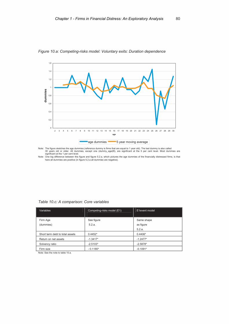
80

Figure 10.a: Competing-risks model: Voluntary exits: Duration dependence

0

0,2

0,4

0,6

0,8

1

1,2

1,4

1,6

2 3 4 5 6 7 8 9 10 11 12 13 14 15 16 17 18 19 20 21 22 23 24 25 26 27 28 29 30

age

dum

mie

s

age dummies 5 year moving average

Note: The figure sketches the age dummies (reference dummy is firms that are equal to 1 year old). The last dummy is also called 30 years old or older. All dummies, except one (dummy_age28), are significant at the 5 per cent level. Most dummies are significant at the 1 per cent level. Note: One big difference between this figure and figure 5.2.a, which pictures the age dummies of the financially distressed firms, is that

here all dummies are positive (in figure 5.2.a all dummies are negative).

Table 10.c: A comparison: Core variables

Variables Competing-risks model (E1)

E1event model

Firm Age

(dummies)

See figure

5.2.a.

Same shape

as figure

5.2.a.

Short term debt to total assets 0.4452* 0.4406*

Return on net assets -1.3417* -1.2477*

Solvency ratio -2.5103* -2.5878*

Firm size - 0.1180* -0.1091* Note: See the note to table 10.a.


81

Table 10.d: A comparison: Proxies

Variables Competing-risks

model (E1)

E1event model

Owned by the public (dummy) 0.1270 (not sign.) 0.0642 (not sign.)

Owned by a fund (dummy) -1.4693 (not sign.) -1.4621 (not sign.)

Diversification 2 sectors (related) (dummy)

Diversification 3–9 sectors (related) (dummy)

Diversification 2 sectors (unrelated) (dummy)

Diversification 3–9 sectors (unrelated) (dummy)

-0.3535*

-0.3933*

-0.2139*

-0.3782*

-0.3472*

-0.3894*

-0.2085*

-0.3753*






-0.3240*

-0.2288*

-0.1195 (not sign)

-0.2010*

-0.3228*

-0.2224*

-0.1169 (not sign.)

-0.1961*

Concentration -0.00317 (not sign.) -0.00353 (not sign.)

Critical comments from the auditors (dummy) 1.0724* 1.0713*

Ultimate parent companies (dummy) 0.3767** 0.3756**

Wholly owned subsidiaries (dummy) -0.3050* -0.3370*



0.4174* 0.4271*



82

11. Appendix: Predictions

Figure 11.a: Firms predicted as non-events: the distribution of the predictions

0

0.002

0.004

0.006

0.008

0.01

0.012

0.014

0.016

0.018

100% 99% 95% 90% 75% 50% 25% 10% 5% 1% 0%

Percentile

Pred

ictio

n

E1event model (non-event) compt.-risks model (non-event)

Figure 11.b: Firms predicted as financially distressed (events): the distribution of the predictions

0

0.2

0.4

0.6

0.8

1

1.2

100% 99% 95% 90% 75% 50% 25% 10% 5% 1% 0%

Percentile

Pred

ictio

n

E1event model (event) compt.-risks model (event)


"Today, there is a near-consensus on the answers in the monetary policy arena. Robert Solow, a Nobel

laureate, once famously titled an article "Faith, Hope and Clarity" – to him, the three most important attributes

to economists. On the framework for financial stability, with a bit of faith there is hope that, perhaps a

generation or two down the road, we will have greater clarity."

Andrew Haldane

CHAPTER 2

1

ANNE DYRBERG ROMMER*

A COMPARATIVE ANALYSIS OF THE DETERMINANTS OF FINANCIAL DISTRESS IN

FRENCH, ITALIAN AND SPANISH FIRMS

* The chapter is based on A. Dyrberg Rommer, 2005, A Comparative Analysis of the Determinants of Financial Distress in French, Italian and Spanish firms, Working Paper no. 28, Danmarks Nationalbank. The chapter has been accepted for presentation at the C.R.E.D.I.T. 2005 Conference on Counterparty Credit Risk, which will take place in Venice on 22-23 September 2005. The author would like to thank Hans Christian Kongsted, Ivan Alves, Jesper Berg, Karsten Biltoft, Olli Castren, Anders Møller Christensen, Frank Dierick, John Fell, Kenneth Juhl Pedersen and Bronka Rzepkowski for commenting on earlier versions of the paper and participants at the European Central Bank seminar, which took place on the 23rd of February 2005. Corresponding address is: Anne Dyrberg Rommer, Financial Markets, Danmarks Nationalbank, Havnegade 5, DK-1093 Copenhagen, Denmark. Phone: + 45 33 63 63 63. Email: [email protected].

2

Abstract

The determinants of corporate failure in Italian, Spanish and French small and medium-sized enterprises are investigated in order to find out whether the predictors of financial distress in the countries are the same or not. There are few studies, which do compare the determinants of financial distress across countries. To the best of our knowledge, this is the first comparative accounting-based credit-rating study of a fairly homogenous group of countries, and so it fills a gap in the literature.

The analysis shows that the factors that drive financial distress in the three analyzed countries are not the same. Hence, the implication for the relevant policy areas – financial stability and Basel II – is that the countries should be analyzed and assessed on an individual basis.

Chapter 2 - A Comparative Analysis of the Determinants of Financial Distressin French, Italian and Spanish firms

3

Table of contents

1. Introduction 4

2. The Literature 6

3. Data and the Hypotheses to be tested 7

3.1 The Construction of the Dependent Variable 7

3.2 Hypotheses 10

3.3 Sample selection 15

3.3.1 Public and private limited liability companies and SMEs 16

3.3.2 Attrition 18 4. Econometric Theory 22

5. Results: The Country Models 24

5.1 Parameter Estimates 24

5.2 Discriminatory Power 28

6. Results: The Country Models compared with a Pooled Model 29

6.1 Parameter Estimates 30

6.2 Discriminatory Power 32

7. Conclusion 33

8. LITERATURE 36

9. Appendix: Other Studies 41

10. Appendix: Legal status codes 44

11. Appendix: Sample Selection in Details 45

12. Appendix: Detailed analysis of the Attritioners 46

12.1 Introduction 46

12.2 Testing for Equal Means of the Explanatory Variables 46

12.3 The Probability of Attrition 55

12.4 Robustness test 63

13. Appendix: Descriptive Statistics 65

14. Appendix: The Construction of Sector Affiliation Codes 74

15. Appendix: Results 75


4

A COMPARATIVE ANALYSIS OF THE DETERMINANTS OF FINANCIAL DISTRESS

IN FRENCH, ITALIAN AND SPANISH FIRMS

1. Introduction

The determinants of corporate failure in Italian, Spanish and French small and medium-sized enterprises (SMEs) are investigated in order to find out whether the predictors of financial distress in the countries are the same or not. In order to compare the determinants of financial distress, accounting-based credit-scoring models for each country are estimated. An accounting-based credit-scoring model is a model, which on the basis of information extracted from company accounts, and perhaps also non-financial information (such as the age of the company), estimates the probability that a particular firm will default on its debt obligations, usually over a one year horizon. Furthermore a model including all countries is estimated. The significant variables and their sign, and its predictive ability is compared to the three country models in order to assess the differences in the determinants of financial distress and in the predictive ability of the two model set ups. There are few studies, which do compare the determinants of financial distress across countries. To the best of our knowledge, this is the first comparative accounting-based credit-rating study of a fairly homogenous group of countries, and so it fills a gap in the literature.

Some of the few studies, which do compare the determinants of failure in several countries, are Hunter and Isachenkova (2000), Bhattacharjee, Higson, Holly and Kattuman (2004) and Ooghe and Balcaen (2002). Hunter and Isachenkova (2000) aim at explaining the differences in predictors of failure in Russian and UK industrial firms. They pick Russian and UK industrial firms, as the results may be useful for the increasing number of western businesses, which export to Russia etc., or for governmental bodies in Russia and international agencies, which provide assistance to Russia. They find that liquidity and gearing are not effective in explaining failure in Russian companies, whereas measures such as size, profitability and turnover seem to be robust predictors. The UK results indicate the importance of profitability, gearing and liquidity. Bhattacharjee et al. (2004) analyse UK and US quoted firms. They set up a competing-risks model to identify the characteristics leading to bankruptcy and acquisition, and they find that there are significant differences in the way in which firms in the UK and US react to changes in the macroeconomic environment. They argue that these differences in response may be attributable to differences in bankruptcy codes in the UK and the US. Another comparative study is Ooghe and Balcaen (2002). Their focus is on whether a given failure prediction model can be easily transferred across countries. Failure prediction models from different countries are


5

compared using a dataset of Belgian company accounts. Their study can be seen as a case study on the “transferability” of models developed in a specific country and period to other countries and/or periods.

Along the lines of Hunter and Isachenkova (2000) and Bhattacharjee et al. (2004) the purpose here is to discuss possible differences and similarities in the determinants of failure in firms in different countries. In contrast to these two other studies, this paper focuses on countries that in important aspects are fairly alike. They all belong to Continental Europe, are a part of the European Monetary Union and they are inspired by the same legal tradition. Furthermore, despite the deregulation and liberalisation process of the financial systems, which took place in the countries in the 1980s and 1990s, banks are still very important sources of financing in all three countries.1 As the countries are fairly alike, a priori, one may think that the same factors drive financial distress in the three countries. One could even argue that if common factors should drive financial distress across countries, it would be in countries that are alike in so many important aspects, such as Spain, Italy and France.

The analysis has implications for at least two policy areas. The first concerns financial stability analysis and the second the Revised Framework for Capital Measurement and Capital Standards, also known as Basel II. An important part of financial stability analysis entails assessing the degree of corporate sector credit risk facing banks.2 For financial stability analysis on a euro area wide basis, it is important to ascertain whether common or country-specific factors drive corporate failures. If the factors that give rise to financial distress are the same across countries, then aggregation of individual corporate sectors into a single group is justified, whereas, if country specific factors are more important, this would call for analysing conditions in each individual corporate sector. Basel II opens up for the possibility that credit institutions themselves can estimate their minimal capital requirements. According to Basel II credit institutions can choose between one of two internal ratings based approaches when they calculate their capital requirements.3 If they choose to do so and follow one of the two internal ratings based approaches they have to calculate the probability of default of their obligors in order to calculate their minimal capital requirements.4 As valid estimates of the probability of default require a considerable amount of data, Basel II allows for banks to pool their data with other banks in order to overcome their data shortcomings, and so a number of international data pooling projects have emerged, where banks from various countries pool their data, c.f. Borup, Kurek and Rommer (2005). Because of this development and as, furthermore, many credit institutions in Europe have cross-border activities, the choice between setting up individual country credit-scoring models or a common credit-scoring model

1 See ECB (2002). 2 Financial stability analysis of non-financial firms usually involves examining conditions in small and medium-sized

enterprises (SMEs) as well as large companies separately. In order to assess the financial health of large companies, a number of information sources are available, such as credit-ratings and market-based indicators such as expected default frequencies. These sources are not available for most SMEs. Instead, the analysis of SMEs usually relies on company accounts. For this study, income statement and balance sheet information was collected for SMEs in France, Italy and Spain.

3 For further details, see Basel Committee on Banking Supervision (2004). 4 This study follows the European Commission definition of SMEs, which differs from the definition of SMEs in Basel II.


6

is relevant, when calculating capital requirements for banks. In order to shed light on these issues, the determinants of corporate failure in French, Italian and Spanish firms are investigated by the estimation of individual country credit-scoring models and a common credit-scoring model.

The paper is structured as follows. Section 2 presents the literature. A discussion of data is found in section 3, which also sets up the hypotheses to be tested. Section 4 presents the econometric theory, and the results are discussed in section 5. Section 6 compares the individual country models with the pooled model. Section 7 concludes.

2. The Literature

Credit-scoring studies using French, Italian and Spanish data are listed in section 9 (appendix). The studies using French data are the following: Bardos (1998) and Bardos (2001) present the Banque de France’s scoring method and discuss the recent developments of the method. Dietsch and Petey (2002) propose a credit model for French SME loans. Moody’s Investors Service (2001b) sets up a country model using data from France. A number of studies use Spanish data. The focus in Jiménez and Saurina (2004) is on the impact of certain loan characteristics on credit risk, e.g. collateral, type of lender institutions and the relationship between the bank and the company it is financing. Corcóstegui, González-Mosquera, Marcelo and Trucharte (2003) estimate a rating system for the Spanish non-financial private-sector firms. Fernandez (1988) estimates a Spanish model for credit risk classification. Moody’s Investors Service (2001a) sets up a country model using data from Spain. There are several studies using Italian data. Cifarelli and Corielle (1988) describe an application of a Baysian variant to discriminant analysis. Altman, Marco and Varetto (1994) analyze the comparison between traditional statistical methodologies for distress classification and prediction with an artificial intelligence algorithm (neural networks). Moody’s Investors Service (2002) sets up a country model using data from Italy.

All the studies differ in terms of sample selection procedure (including period covered and default definition) and econometric technique. None of them are of a comparative nature. In fact, very few studies compare the determinants of failure across countries. As mentioned in the introduction, some of the few studies, which do compare the determinants of failure in several countries, are Hunter and Isachenkova (2000) and Bhattacharjee et al. (2004). The studies, which analyse Russian firms and UK firms and firms in the UK and US, respectively, differ from this study, whose focus is on a fairly homogenous group of countries.

Various estimation techniques have been suggested in the accounting-based credit-scoring literature (e.g. discriminant analysis and the logit model).5 When estimating a credit-scoring model, typically, information on two groups of firms is gathered and used in the estimations, namely information on

5 For an overview of the literature the reader is referred to Lando (2004). Some of the often quoted accounting-based credit-

scoring studies are Beaver (1966), Altman (1968), Ohlson (1980) and Shumway (2001).


7

firms in financial distress and active firms. Along the lines of Dyrberg (2004), this paper extends the common practice in credit-rating studies and it includes also firms that exit for other reasons than financial distress (e.g. voluntary liquidations). As firms can exit for various reasons a competing-risks model is set up. The estimation strategy of Allison (1982) is followed and the probability of exiting to the various states is estimated simultaneously. Methodologically related papers are Harhoff, Stahl and Woyde (1998), Köke (2001), Prantl (2003) and Bhattacharjee et al. (2004). All four studies distinguish between two forms of exit. Harhoff et al. (1998) and Prantl (2003) model voluntary liquidations and bankruptcies in Germany using a competing-risks framework. Bhattacharjee et al. (2004) use a competing-risks model to identify the characteristics leading to bankruptcy and acquisition in UK and US quoted firms. Köke (2001) investigates the determinants of acquisition and failure in Germany. He provides stylized facts and discusses lessons for empirical studies of firms.

3. Data and the Hypotheses to be tested

This section discusses the dataset used in the estimations, including the construction of the dependent variable and the sample selection criteria, and it sets up hypotheses to be tested.

3.1 Construction of the Dependent Variable

The data used for Italy, Spain and France comes from the harmonised Amadeus database, which is a pan-European database, provided by Bureau van Dijk (BvD).6 As opposed to most Italian, Spanish and French credit-scoring models presented in the literature, which use non-public information from credit registries operated by governments (usually by bank supervisors) or from other non-public sources, c.f. section 9 (appendix), this study uses public information only. The great virtue of the data set is that it enables us to make cross-country comparisons. On the negative side it should be mentioned that the data set, when looking at each country individually, is not as good as some of the data sets used in the individual country studies (in the sense that a number of firms drop out of the panel with no explanation).

Amadeus contains information on public and private companies. A standard company report includes balance sheet items, profit and loss account items and non-financial information such as BvD ID number, address, legal status, date of incorporation, sector affiliation code, number of employees,

6 The data is loaded from the Amadeus cd-roms dated September 2004, October 2004 and November 2004. Working with the

Amadeus database has delivered one important by-product for other studies taking their point of departure in the database. We investigated whether or not the analysis could be done for Germany, but it could not. The reason is that Creditreform, who provides German data to Amadeus, only delivers company accounts for the “best” German firms. Creditreform divides the German financial accounts into 6 different risk classes. The four best classes are included in Amadeus. The two worst classes are not included. These last two classes include defaulting firms, and so, if one wants to estimate a credit-scoring model, one cannot do this from the data in Amadeus only. This finding, which is not described in the Amadeus documentation, is important for other studies as well. One needs to be aware of the fact that only relatively “good” German financial accounts can be obtained from Amadeus. The sample is not representative.


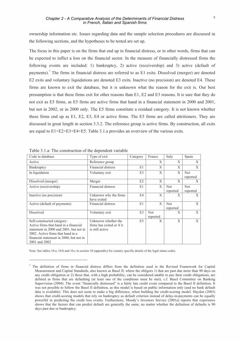
8

ownership information etc. Issues regarding data and the sample selection procedures are discussed in the following sections, and the hypotheses to be tested are set up.

The focus in this paper is on the firms that end up in financial distress, or in other words, firms that can be expected to inflict a loss on the financial sector. In the measure of financially distressed firms the following events are included: 1) bankruptcy, 2) active (receivership) and 3) active (default of payments).7 The firms in financial distress are referred to as E1 exits. Dissolved (merger) are denoted E2 exits and voluntary liquidations are denoted E3 exits. Inactive (no precision) are denoted E4. These firms are known to exit the database, but it is unknown what the reason for the exit is. Our best presumption is that these firms exit for other reasons than E1, E2 and E3 reasons. It is sure that they do not exit as E5 firms, as E5 firms are active firms that hand in a financial statement in 2000 and 2001, but not in 2002, or in 2000 only. The E5 firms constitute a residual category. It is not known whether these firms end up as E1, E2, E3, E4 or active firms. The E5 firms are called attritioners. They are discussed in great length in section 3.3.2. The reference group is active firms. By construction, all exits are equal to E1+E2+E3+E4+E5. Table 3.1.a provides an overview of the various exits.

Table 3.1.a: The construction of the dependent variable Code in database Type of exit Category France Italy Spain Active Reference group X X X Bankruptcy Financial distress E1 X X X In liquidation Voluntary exit E3 X X Not

reported Dissolved (merger) Merger E2 X X X Active (receivership) Financial distress E1 X Not

reported Not reported

Inactive (no precision) Unknown why the firms have exited

E4 X X X

Active (default of payments) Financial distress E1 X Not reported

X

Dissolved Voluntary exit E3 Not reported

X X

Self-constructed category: Active firms that hand in a financial statement in 2000 and 2001, but not in 2002. Active firms that hand in a financial statement in 2000, but not in 2001 and 2002

Unknown whether the firms has exited or if it is still active

E5 X X X

Note: See tables 10.a, 10.b and 10.c in section 10 (appendix) for country specific details of the legal status codes.

7 The definition of firms in financial distress differs from the definition used in the Revised Framework for Capital

Measurement and Capital Standards, also known as Basel II, where the obligors 1) that are past due more than 90 days on any credit obligation or 2) those that, with a high probability, can be considered unable to pay their credit obligations, are defined as firms that are defaulting (at least one of the conditions must be met), c.f. Basel Committee on Banking Supervision (2004). The event “financially distressed” is a fairly late credit event compared to the Basel II definition. It was not possible to follow the Basel II definition, as this model is based on public information only (and no bank default data is available). This does not seem to make a big difference, when building the credit-scoring model. Hayden (2003) shows that credit-scoring models that rely on bankruptcy as default criterion instead of delay-in-payments can be equally powerful in predicting the credit loss events. Furthermore, Moody’s Investors Service (2001a) reports that experience shows that the factors that can predict default are generally the same, no matter whether the definition of defaults is 90 days past due or bankruptcy.


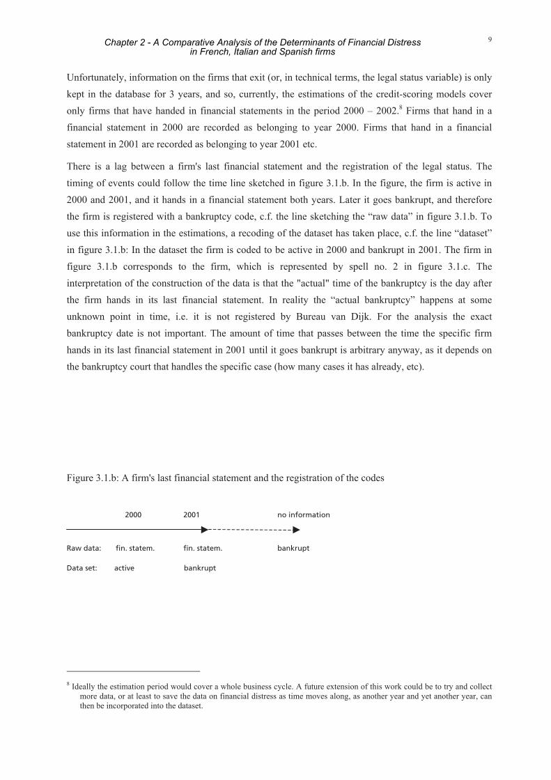
9

Unfortunately, information on the firms that exit (or, in technical terms, the legal status variable) is only kept in the database for 3 years, and so, currently, the estimations of the credit-scoring models cover only firms that have handed in financial statements in the period 2000 – 2002.8 Firms that hand in a financial statement in 2000 are recorded as belonging to year 2000. Firms that hand in a financial statement in 2001 are recorded as belonging to year 2001 etc.

There is a lag between a firm's last financial statement and the registration of the legal status. The timing of events could follow the time line sketched in figure 3.1.b. In the figure, the firm is active in 2000 and 2001, and it hands in a financial statement both years. Later it goes bankrupt, and therefore the firm is registered with a bankruptcy code, c.f. the line sketching the “raw data” in figure 3.1.b. To use this information in the estimations, a recoding of the dataset has taken place, c.f. the line “dataset” in figure 3.1.b: In the dataset the firm is coded to be active in 2000 and bankrupt in 2001. The firm in figure 3.1.b corresponds to the firm, which is represented by spell no. 2 in figure 3.1.c. The interpretation of the construction of the data is that the "actual" time of the bankruptcy is the day after the firm hands in its last financial statement. In reality the “actual bankruptcy” happens at some unknown point in time, i.e. it is not registered by Bureau van Dijk. For the analysis the exact bankruptcy date is not important. The amount of time that passes between the time the specific firm hands in its last financial statement in 2001 until it goes bankrupt is arbitrary anyway, as it depends on the bankruptcy court that handles the specific case (how many cases it has already, etc).

Figure 3.1.b: A firm's last financial statement and the registration of the codes

2000 2001 no information

Raw data: fin. statem. fin. statem. bankrupt

Data set: active bankrupt

8 Ideally the estimation period would cover a whole business cycle. A future extension of this work could be to try and collect

more data, or at least to save the data on financial distress as time moves along, as another year and yet another year, can then be incorporated into the dataset.


10

Figure 3.1.c: Observation window (5 examples of firms that are used in the analysis)

No. 1

No. 2

No. 3

No. 4

No. 5

… 1999 2000 2001 2002 2003 … Note: The data set consists of a single spell for each firm, meaning that once a firm has exited it cannot re-enter. This figure pictures five different spells (see the arrows in the figure). Each firm is observed when it hands in its financial statement in 2000, 2001 and 2002 (if it does not exit during the period). The period 2000 to 2002 is called the observation window. As the firms are observed once a year, but interact on a continuous basis, the data is called grouped duration data. The data set consists of firms that are both flow and stock sampled. Spell no. 1 and 3 are flow sampled and spell no. 2, 4 and 5 are stock sampled. The firms that enter the active state in the period of interest (in 2000, 2001 or 2002) are flow sampled. The firms that are already active in 2000 are stock sampled. The firms are censored in various ways (as they are only observed in the observation window). Stock sampled firms can be left censored, left truncated and right censored. They are left censored, if the incorporation data is unknown. They are left truncated, if the incorporation data is known. The firms that survive beyond the observation window are right censored, as they are not observed after the end of the observation window. The flow sampled firms are not left censored (or left truncated) as their history is observed from the beginning of the spell. The flow sampled firms that survive beyond the observations window are right censored, as they are not observed after the end of the observation window.

3.2 Hypotheses

A number of hypotheses, that are to be tested, are set up in this section. The focus is on the way various factors may affect the likelihood of exiting as an E1 firm. No hypothesis will be set up on the effect of the institutional framework. Spain, Italy and France are all French-civil law countries9, and so large differences between the institutional frameworks are not present, c.f. table 3.2.a., which shows how the countries do on enforcement variables (e.g. “efficiency of judicial system”, “rule of law” and

9 La Porta et al. (1998) discuss the rules and practices governing the resolution of financial distress in 49 countries. Their focus

is on company and bankruptcy/reorganization laws. They explain how commercial laws come from two broad traditions. One tradition is the common-law family, which is English in origin. The other tradition is civil law, which derives from Roman law. Within the civil tradition, the modern commercial laws can have French, German, and Scandinavian origin. The French Commercial Code, which Italy, Spain and France are inspired by, dates back to Napoleon in 1807. The German Commercial code was written in 1897 after Bismarck’s unification of Germany. The Scandinavian laws are “similar to each other but “distinct” from others” (La Porta et al. (1998:1119)). This study focuses on France, Italy and Spain, which are inspired by the French Commercial Code. Examples of credit-scoring studies that take their point of departure in the other law families are Bunn and Redwood (2003) (common-law family), Scheule (2003) (German origin) and Dyrberg (2004) (Scandinavian origin).


11

“corruption”), accounting standards and creditor rights (e.g. “no automatic stay on assets”, “secured creditors paid first”). Table 3.2.a shows, that the three countries do better on the enforcement variables and on the rating on accounting standards than the French-civil average (which is calculated on the basis of all French-civil law countries studied in La Porta et al. (1998) and not only on the basis of France, Italy and Spain)10, but, that France does worse than the French-civil average when measured on creditor rights11. These issues will not be addressed further. Instead it will be discussed how other factors, which possibly are affected by the rules and practices governing the resolution of customers’ financial distress, may explain, why different determinants of financial distress in the countries end up being significant in the estimations. First, the common indicators in credit-scoring models – profitability, solvency, leverage, age and size – are discussed. Thereafter, various proxies, which are used for the inherently unobservable variables, are discussed. All variables are listed in table 3.2.b.

Hypothesis 1 concerns the effect of profitability (measured as the earnings ratio, here defined as EBITDA (earnings before interest, taxes, depreciation and amortization) to total assets). The hypothesis is that the sign of the coefficient to the earnings ratio is negative in all countries. Hypothesis 2 concerns the solvency ratio, which expresses the firm’s ability to generate satisfactory earnings over time. It is calculated as shareholders funds over total assets, and it can be seen as a buffer. The hypothesis for all countries is that a high solvency ratio decreases the probability of moving into financial distress. Hypothesis 3 concerns the leverage measured as loans over total assets.12 The hypothesis is that higher leverage increases the probability of moving into financial distress.

Hypothesis 4 and 5 concerns the size and the age of the firms. As these variables are correlated (e.g. because older firms tend to be larger than younger firms) it can be difficult to disentangle the effects stemming from age and size. Hypothesis 4 concerns the size of a firm, which is measured as the logarithm of total assets. The hypothesis is that the larger the firm is, the less likely it is to enter financial distress. Hypothesis 5: Age is also included in the estimations. Dummies for each age are included (1 year old firms are chosen as the reference group). In the final results, only significant age dummies are presented. The hypothesis is that the older the firm is, the less likely it is to enter financial distress.

Hypothesis 6 concerns a proxy for diversification, namely a variable, which measures the number of subsidiaries attached to the specific company. It is left to the estimations to show whether or not there is a significant effect of this variable.

10 Except one variable for Spain: The enforcement variable “efficiency of judicial system” is lower for Spain than the French-

origin average. 11 Note also that the legal reserve required as a percentage of capital in the three countries is smaller than the French-origin

average. 12 In the Amadeus database, current liabilities are split up on loans, creditors and other current liabilities. To construct the

leverage measure, the loans item is used.


12

Table 3.2.a: Enforcement variables, rating on accounting standards and creditor rights (higher score is better enforcement, accounting standards and creditor rights, respectively) France Italy Spain French-origin

average

Efficiency of Judicial System

8.00 6.75 6.25 6.56

Rule of Law 8.98 8.33 7.80 6.05

Corruption 9.05 6.13 7.38 5.84

Risk of Expropriation 9.65 9.35 9.52 7.46

Enforcement variables

Risk of contract Repudiation

9.19 9.17 8.40 6.84

Accounting standards

Rating on accounting standards

69 62 64 51.17

No automatic stay on assets

0 0 1 0.26

Secured creditors first paid 0 1 1 0.65

Restrictions for going into reorganization

0 1 0 0.42

Management does not stay in reorganization

0 0 0 0.26

Creditor rights, sum 0 2 2 1.58

Creditor rights (1=creditor protection is the law)

Legal reserve required as a percentage of capital

0.10 0.20 0.20 0.21

Note: The French-civil average consist of Argentina, Belgium, Brazil, Chile, Colombia, Ecuador, Egypt, France, Greece, Indonesia, Italy, Jordan, Mexico, Netherlands, Peru, Philippines, Portugal, Spain, Turkey, Uruguay and Venezuela. Enforcement variables: Efficiency of judicial system. Assessment of the “efficiency and integrity of the legal environment as it affects business, particularly foreign firms’” produced by the country risk rating agency Business International Corp. It “may be taken to represent investors’ assessments of conditions in the country in question.“ Scale from zero to 10; with lower scores, lower efficiency levels. Rule of law. Assessment of the law and order tradition in the country produced by the country risk rating agency International Country Risk (ICR). Scale from zero to 10, with lower scores for less tradition for law and order. Corruption. ICR’s assessment of the corruption in government. Lower scores indicate that “high government officials are likely to demand special payments” and “illegal payments are generally expected throughout lower levels of government” in the form of “bribes connected with import and export licences, exchange controls, tax assessment, policy protection, or loans.” Scale from zero to 10, with lower scores for higher levels of corruption. Risk of expropriation. ICR’s assessment of the risk of “outright confiscation” or “forced nationalisation”. Scale from zero to 10, with lower scores for higher risks. Risk of contract repudiation. ICR’s assessment of the “risk of a modification in a contract taking the form of a repudiation, postponement, or scaling down” due to “budget cut-backs, indigenization pressure, a change in government, or a change in economic and social priorities”. Scale from zero to 10, with lower scores for higher risks. Accounting standards. Index created by examining and rating companies’ annual reports on their inclusion or omission of 90 items. These items fall into seven categories (general information, income statements, balance sheets, funds flow statement, accounting standards, stock data, and special items). A minimum of three companies in each country were studied. Creditor rights. Restrictions for going into reorganisation equals one if the reorganisation procedure imposes restrictions, such as creditors’ consent, to file for reorganisation; equals zero if there are no such restrictions. No automatic stay on secured assets equals one if the reorganisation procedure does not impose an automatic stay on the assets of the firm on filing the reorganisation petition. Secured creditors’ paid first equals one if secured creditors are ranked first in the distribution of the proceeds that result from the disposition of the assets of a bankrupt firm; equals zero if non-secured creditors, such as the government and workers, are given absolute priority. Management does not stay equals one when an official appointed by the court, or by the creditors, is responsible for the operation of the business during reorganization. Equivalently, this variable equals one if the debtor does not keep the administration of its property pending the resolution of the reorganization process. Equals zero otherwise. Creditor rights is an index aggregating different creditor rights. The index is formed by adding 1 when (1) the country imposes restrictions, such as creditors’ consent or minimum dividends to file for reorganisation; (2) secured creditors are able to gain possession of their security once the reorganization petition has been approved (no automatic stay); (3) secured creditors are ranked first in the distribution of the proceeds that results from the disposition of the assets of a bankrupt firm; and (4) the debtor does not retain the administration of its property pending the resolution of the reorganization. The index ranges from zero to four. Legal reserve. The minimum percentage of total share capital mandated by corporate law to avoid the dissolution of an existing firm. It takes a value of zero for countries without such a restriction.

Source: La Porta et al. (1998)


13

Table 3.2.b: The explanatory variables used in the study Variable

Profitability: Earnings ratio= EBITDA/total assets. EBITDA = earnings before interest, taxes, depreciation and

amortization

Solvency: Solvency = Shareholders funds/total assets

Leverage: Loans/total assets

Firms size: Log(total assets)

Core

variables

Age: Dummies. Reference category is firms that are 1 year old.

Subsidiaries: This variable measures the number of subsidiaries that a company has registered.

Legal form: This dummy is equal to 1, if it is a private limited liability company, and equal to 0, if it is a public

limited liability company.

Shareholders: This variable measures the number of recorded shareholders.

Proxies

Independence indicator: Three dummies are included. The first is equal to 1 when it is a type A firm

(bvd_indep_a), the second is equal to 1 when it is a type B firm (bvd_indep_b) and the third is equal to one when

it is a type C firm (bvd_indep_c). Reference category is type U firms. See text for more details.

Macroeconomic environment: Year dummies are included. The reference year is 2000. Controls

Sector affiliation dummies: Dummies for the following sectors are included (see section 14 (appendix)):

Farming, Forestry, Fishing, Mining, Manufacturing (reference dummy), Energy, Construction, Trade and hotel,

Transport, Business service, Public service activities, Organisations. The following abbreviations are used.

Dumfar = Farming, forestry and fishing, Dummin = Mining, Dumman= Manufacturing, Dumener = Energy,

Dumcon = Construction, Dumtraho = Trade and hotel, Dumtra = Transport, Dumbus = Business service,

Dumpub = Public service activities, Dumorg = Organisations. As there are no NACE codes for the IT and tele-

sector a (self-constructed) IT and tele-dummy is included in the estimations. On top of belonging to one of the

above sectors a firm is considered to be in the IT and tele group if it has activities in one of the sectors listed in

table 14.b in section 14 (appendix).

Hypothesis 7: Legal form is used as a proxy for willingness to take on risk. The legal form dummy is constructed such that for all countries, the dummy is equal to one, when the legal form of the company is a private limited liability company, and it is equal to zero, when it is a public limited liability company. One would think that private limited liability companies would be more risky, as they would have less share capital to loose compared with public limited liability companies, and so the variable is hypothesized to have a positive sign.13

13 The terms public and private limited liability companies are used to denote the law the specific company is following. There

are different rules for public and private limited liability companies, i.e. concerning the amount of share capital that they need to hold. Note that not all public limited liability companies are listed on a stock exchange.


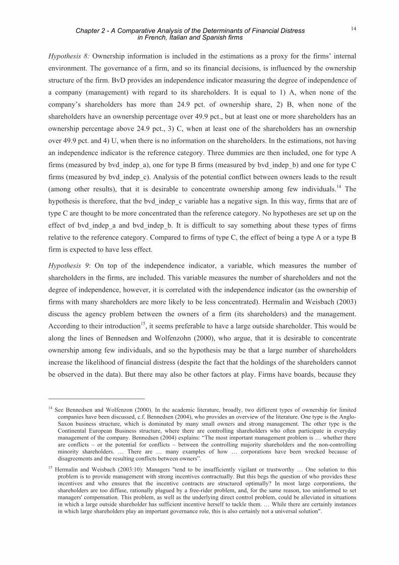
14

Hypothesis 8: Ownership information is included in the estimations as a proxy for the firms’ internal environment. The governance of a firm, and so its financial decisions, is influenced by the ownership structure of the firm. BvD provides an independence indicator measuring the degree of independence of a company (management) with regard to its shareholders. It is equal to 1) A, when none of the company’s shareholders has more than 24.9 pct. of ownership share, 2) B, when none of the shareholders have an ownership percentage over 49.9 pct., but at least one or more shareholders has an ownership percentage above 24.9 pct., 3) C, when at least one of the shareholders has an ownership over 49.9 pct. and 4) U, when there is no information on the shareholders. In the estimations, not having an independence indicator is the reference category. Three dummies are then included, one for type A firms (measured by bvd_indep_a), one for type B firms (measured by bvd_indep_b) and one for type C firms (measured by bvd_indep_c). Analysis of the potential conflict between owners leads to the result (among other results), that it is desirable to concentrate ownership among few individuals.14 The hypothesis is therefore, that the bvd_indep_c variable has a negative sign. In this way, firms that are of type C are thought to be more concentrated than the reference category. No hypotheses are set up on the effect of bvd_indep_a and bvd_indep_b. It is difficult to say something about these types of firms relative to the reference category. Compared to firms of type C, the effect of being a type A or a type B firm is expected to have less effect.

Hypothesis 9: On top of the independence indicator, a variable, which measures the number of shareholders in the firms, are included. This variable measures the number of shareholders and not the degree of independence, however, it is correlated with the independence indicator (as the ownership of firms with many shareholders are more likely to be less concentrated). Hermalin and Weisbach (2003) discuss the agency problem between the owners of a firm (its shareholders) and the management. According to their introduction15, it seems preferable to have a large outside shareholder. This would be along the lines of Bennedsen and Wolfenzohn (2000), who argue, that it is desirable to concentrate ownership among few individuals, and so the hypothesis may be that a large number of shareholders increase the likelihood of financial distress (despite the fact that the holdings of the shareholders cannot be observed in the data). But there may also be other factors at play. Firms have boards, because they

14 See Bennedsen and Wolfenzon (2000). In the academic literature, broadly, two different types of ownership for limited

companies have been discussed, c.f. Bennedsen (2004), who provides an overview of the literature. One type is the Anglo-Saxon business structure, which is dominated by many small owners and strong management. The other type is the Continental European Business structure, where there are controlling shareholders who often participate in everyday management of the company. Bennedsen (2004) explains: “The most important management problem is … whether there are conflicts – or the potential for conflicts – between the controlling majority shareholders and the non-controlling minority shareholders. … There are … many examples of how … corporations have been wrecked because of disagreements and the resulting conflicts between owners”.

15 Hermalin and Weisbach (2003:10): Managers "tend to be insufficiently vigilant or trustworthy … One solution to this problem is to provide management with strong incentives contractually. But this begs the question of who provides these incentives and who ensures that the incentive contracts are structured optimally? In most large corporations, the shareholders are too diffuse, rationally plagued by a free-rider problem, and, for the same reason, too uninformed to set managers' compensation. This problem, as well as the underlying direct control problem, could be alleviated in situations in which a large outside shareholder has sufficient incentive herself to tackle them. … While there are certainly instances in which large shareholders play an important governance role, this is also certainly not a universal solution".


15

are "part of the equilibrium solution to the contracting problem between diffuse shareholders and management", (Hermalin and Weisbach (2003:10)). As there is no information on boards in the dataset and no clear hypothesis can be set up on the effect on the number of shareholders, it will be left to the estimations to show the effect of this variable.

Sector affiliation dummies are included to control for the sector affiliation of the firms. The reference category is firms in the manufacturing sector. Furthermore, year dummies are included to control for business cycle effects. The reference year is 2000.

3.3 Sample selection

The construction of the sample used in the estimations is discussed in this section. The sample selection criteria are summarized in table 3.3, which is split up on conceptual criteria and other criteria.16 After the application of the criteria, the database consists of a total of 282,131 firm-year observations (FR: 108,533, IT: 97,732, ES: 75,866) covering the years 2000 - 2002. The proportion of SMEs in financial distress to the overall number of SME firm-years is 0.2 per cent in Spain and Italy and 1.6 per cent in the French case.17 Despite the differences in levels, it is the assessment, that we have a random sample, and accordingly, that the estimations are consistent across countries and that the effects of the explanatory variables in the various countries can be meaningfully compared. Descriptive statistics are found in section 13 (appendix).

Most of the sample selection criteria are self-explanatory. Nonetheless, in the following sections, it is discussed why only public and private limited liability companies have been considered and why it was chosen to focus only on SMEs. Furthermore, the attrition problem is discussed.

16 See section 11 (appendix) for details. 17 To benchmark the French, Spanish and Italian data, they are compared to a sample of Danish SME’s, which covers the

whole population of Danish public and private limited liability companies. The sample is analysed and discussed extensively in Dyrberg (2004). In this sample of Danish firms, the proportion of E1 events is 0.8 per cent, which is higher than the fraction in Italy and Spain and lower than fraction in France. Compared to the dataset used in Dyrberg (2004) the following corrections are made in order to make the figures comparable: Only SMEs are considered and the E1 measure is modified to be comparable to the E1 measure used in this paper. The Danish data set includes bankruptcies in the period 1995 – 2001. The dataset for the other countries covers the period 2000 – 2002.


16

Table 3.3: Sample selection criteria Criteria

Only unconsolidated statements are analysed.

Financial institutions and non-financial holding companies are excluded.

Only public limited liabilities and private limited liabilities are analysed.

Only SMEs are analysed.

Conceptual

Some firms leave with no explanation (that is, they are not assigned an exit code). These firms are called attritioners. They are denoted E5. They are excluded from the estimations based on bvd_id.

If a company hands in two financial statements in one year, only the last financial statement is included in the estimations.

Active companies are excluded if they hand in a financial statement in 2000 and 2002 only.

Various corrections are made to the database (e.g. firms with illogical variables, such as short-term debt less than zero and a solvency ratio larger than 100 pct., are excluded).

Other

Firms with missing variables on any of the explanatory variables are excluded.

3.3.1 Public and private limited liability companies and SMEs

In this section it is discussed how it is ensured that we have a homogenous group of firms across countries.

A study on bankruptcies and the legal consequences of bankruptcies is provided by the European Commission (2003a). The work takes its point of departure in the Principles and Guidelines for Effective Insolvency and Creditor Rights Systems, which were developed by the World Bank to promote an international consensus on a framework to assess the effectiveness of insolvency and creditor rights systems.18 Attached to the European Commission (2003a) study are country studies, which among other things include detailed discussions of the accounting standards in the countries, c.f. European Commission (2003b, 2003c and 2003d). These discussions are reviewed in this section. The overall conclusion is that there are many nuances in the countries, but that it makes sense to distinguish a homogenous group of firms across countries, namely SMEs that are either private or public limited liability companies.

18 The European Commission set up an expert group in 2002 to take part in a benchmarking exercise chaired by the

Commission. It consisted of experts from 14 Member States, 7 Candidate Countries and Norway. The European Commission (2003a:321) points out that the “results of the … questionnaires that we received from our experts are to be taken carefully and to be considered as nothing more than what they really reflect: the opinion of … national experts regarding the implementation of the World Bank principles in their own legal systems, based on their high experience in the matter of insolvency. Accordingly, we believe that it is interesting to show and to describe practices throughout the EU Member States and the U.S. regarding the World Bank principles, as they are perceived by the national experts. Nevertheless, we are aware that their results cannot necessarily be extended or generalized, and that is the reason why we would not affirm Member States that have the highest rate of implementation should be showed as examples of best practice.” According to the study, out of the three analysed studies, Spain has the largest number of principles not adopted. France and Italy come out similarly.


17

In France, public limited liability companies (“société par action”19), private limited liability companies (“société à responsabilité limitée”) and partnerships (“société en nom collectif”) must file annual accounts and an annual report with the clerk of the Commercial Court and they are subject to criminal penalties in case of violation (European Commission (2003d:3f)).

In Italy, public limited liability companies (“Società par Azoni”) and private limited liability companies (“Società a Responsabilità Limitata”), whose share capital is equal to or higher than 100,000 euro or companies who for two years has not provided the duly publication of the balance sheets required by law, are supervised by a board of internal auditors. The board has the task to control the management of the company in order to safeguard the interest of the shareholders and creditors of the company. It is “… constituted by professionals registered with the Roll of Certified Accountants and appointed by the shareholders, shall supervise the management of the company, the compliance by the other corporate bodies with applicable legal and statutory rules and it controls that the company’s accounts are regularly kept, that the balance sheet reflects the situation resulting from the company’s accountancy books and that the rules established for the evaluation of the company’s assets are complied with”, c.f. European Commission (2003b:7).

In Spain, the filing is mandatory for public limited liability companies (“Sociedad Anonima”) and private limited liability companies (“Sociedad Limitada”).20 Despite the rules, there are quite a number of companies, which do not comply with the annual accounts record obligation (European Commission (2003c:10)). One could fear that the weaker firms are the ones that are not handing in their financial statement. If this is true, the estimates for Spain would be conservative compared to the actual situation. Having this in mind, one could choose to focus on audited firms only. In Spain, firms whose turnover exceeds 4.75 million euros, whose total assets exceed 2.37 million euros and whose total number of workers exceeds 50 during two consecutive years, are obliged to audit their financial statements.21

Table 3.3.1: The definition of micro, small and medium-sized enterprises Category Employees Turnover OR Total balance sheet

Micro enterprises <10 <= 2 million euro OR <= 2 million euro

Micro and Small enterprises <50 <= 10 million euro OR <= 10 million euro

Micro, Small and Medium-sized enterprises <250 <= 50 million euro OR <= 43 million euro

Note: A further criterion for being an SME according to the European Commission definition concerns the economic power of the enterprise. According to the European Commission a distinction should be made between various types of enterprises, depending on whether they are autonomous, whether they have holdings, which do not entail a controlling position or whether they are linked to other enterprises. For an SME to be considered autonomous, less than 25 pct. capital shares should be held by third party. This criterion is not taken into account in the construction of the SME sample. Instead an independence indicator is included in the estimations. Source: European Commission (2003e).

19 In the French country study, the expression “Société par action” is used to denote public limited liability companies.

“Société par action” is not a legal form itself, but comprises of a set of companies, including “société anonyme à conseil d’administration”, “société anonyme à directoire” and “société par actions simplifiée”.

20 Information is provided from Informa S.A. in October 2004. Informa S.A. provides Spanish data to Amadeus. 21 We would like to thank Antonio Marcelo for pointing this out and for providing us with the information. The information is

as of September 2004.


18

To address the potential problem with the financial statements from Spanish firms, it was decided to follow the European Commission definition of SMEs (see table 3.3.1) and to stick to this definition for all countries. According to the SME lower bound criterion firms with at least 10 employees and with total assets of at least 2 million euro are included in the sample.22 It is not as strict as the criterion for when Spanish firms should be audited. Nonetheless, the criterion does accommodate the critique posed by Creditreform. According to Creditreform (2003:16 and 2002:8), micro-companies cannot file for bankruptcy in Spain, and companies, which can no longer pay their bills, are not brought to court by their creditors, as the relevant proceedings are too elaborate and too costly to the creditors to justify the effort involved. Creditreform (2002:8) notes: “To permit a real comparison with, say, Germany, all those cases rejected in this country for lack of sufficient assets to justify proceedings would have to be omitted from the statistics.” The criterion ensures that micro-companies, which resemble households, are excluded from the sample, and furthermore, that only “truly” active companies are analysed. The upper bound criterion ensures that the analysed group of firms is fairly homogenous.

To align the analysed group of French companies with the group of Spanish and Italian companies, which do not include partnerships, only French, Italian and Spanish public limited liability companies and private limited liability companies are analysed.

3.3.2 Attrition

The fact that some firms leave with no explanation (that is, they are not assigned an exit code), is called attrition. It is crucial to find out whether or not attrition is a problem. If there is a selection bias, i.e. a distortion of the estimation results due to non-random patterns of attrition, we need to correct for this.23

This section starts out discussing the extent of the attrition problem and by explaining why the drop-outs could potentially be a problem for the analysis. Afterwards the various types of drop-outs discussed in the literature are briefly reviewed.

22 The criteria are applied to the firms the year they are included in the database. This means, that the position of the firms can

be deteriorating once they are included. 23 Attrition is a common problem seen in many panel data studies. Accordingly how to treat attrition in panel data models is

discussed in a number of articles, c.f. the discussion of attrition in Wooldridge (2002:585ff) and the Journal of Human Resources (Spring 1998), which has a special issue devoted to the topic. Alderman, Behrman, Kohler, Maluccio and Watkins (2000) summarize the conclusion from the papers in The Journal of Human Resources with the words: “The striking result of these studies is that the biases in estimated socioeconomic relations due to attrition are small – despite attrition rates as high as 50 percent and with significant differences between the means of a number of outcome and standard control variables”. This is an interesting conclusion that they themselves also obtain in their own study, in which they discuss the extent and implications of attrition in three longitudinal household surveys from Bolivia, Kenya and South Africa, which all report very high per-year attrition rates between survey rounds. The attrition rates are considerable: 35 percent for the Bolivian sample, between 28 percent for women to 41 percent for couples in the Kenyan sample and form 16 percent for households to 22 percent for preschool children in the South African sample (Alderman et al. (2000:12)). The conclusion in Alderman et al. (2000:24) is that “…in contrast to often-expressed concerns about attrition, for many estimates the coefficients on standards variables in equations are unaffected by attrition … Thus, even when attrition is fairly high, as it is in the samples we used, attrition apparently is not a general and pervasive problem for obtaining consistent estimates.”. This being said, it is stressed in the paper, that, as a general observation, analysts should assess the problem for the particular model and the particular data that is used.


19

The extent of the attrition problem in the dataset is seen from tables 3.3.2.a, 3.3.2.b and 3.3.2.c. The tables give an overview of the data, when all sample selection criteria, except the attrition sample selection criteria, are taken into account (see table 3.3 in section 3.3). Table 3.3.2.a shows, that in 2000, 73 Italian firms left the database because of an E1 event, 6 firms left the database because of an E2 event, 117 firms left the database because of an E3 event etc. Throughout the whole period (2000 – 2002), a total of 218 Italian firms left the dataset because of financial distress (E1 event), 24 firms left because of mergers (E2 event), 439 firms left because they are voluntarily liquidated (E3 event) etc. It is important to note that 5,201 Italian firms are recorded as E5 firms (total). 1,278 Italian firms are “lost” between 2000 and 2001, and so they are recorded as E5 firms in 2000, and 3,923 firms are “lost” between 2001 and 2002, and so they are recorded as E5 firms in 2001. The E5 firms belong to the category “unknown whether the firm has exited or if it is still active”. The only thing, which is known about these firms, is that they are no longer observed in the database. The firms that are recorded as E5 firms in year 2000 are no longer observed in the years 2001 and 2002. The firms that are recorded as E5 firms in year 2001 are no longer observed in year 2002. The recording of E5 firms is zero for 2002, as no firm is known to be lost after 2002 (as the dataset stops in 2002). The E5 firms are called attritioners. The fact that they leave the panel (with no explanation) is called attrition.

Table 3.3.2.a: Italy: E1, E2, E3, E4, E5 and active firms 2000 2001 2002 Total

E1 73 72 10 155

E2 6 2 16 24

E3 117 74 248 439

E4 9 10 46 65

E5 1278 3923 0 5201

Active 31316 32989 35977 100282

Total 32799 37070 36297 106166

Table 3.3.2.b: Spain: E1, E2, E3, E4, E5 and active firms 2000 2001 2002 Total

E1 65 64 51 180

E2 31 41 23 95

E3 272 301 344 917

E4 8 15 27 50

E5 519 2204 0 2723

Active 21586 25260 29349 76195

Total 22481 27885 29794 80160


20

Table 3.3.2.c: France: E1, E2, E3, E4, E5 and active firms 2000 2001 2002 Total

E1 167 396 1140 1703

E2 48 686 675 1409

E3 2 22 39 63

E4 152 418 525 1095

E5 873 2490 0 3364

Active 30281 34710 40796 105787

Total 31523 38722 43175 113420

One could have two opposing hypotheses of why some firms drop-out for unknown reasons (the E5 firms). Hypothesis 1: The first hypothesis is that Bureau van Dijk (BvD) does not care about the firms, when they are no longer active, and therefore that it is not sure that all non-active firms get an exit code. Note, however, that if BvD want to track the bankrupt firms, it should not be difficult, as the names of the firms that have gone bankrupt are usually published. Hypothesis 2: The other hypothesis is that the firms that drop out for unknown reasons are likely to be active firms, as firms that exit because of financial distress are easier to track than active firms. For statisticians it can be a really time-consuming task to trace active firms that change legal form or for other reasons re-register, c.f. Statistics Denmark (2002) and Eurostat (2004). If the active firms in Spain, Italy and France change legal status or for other reasons are registered in another way, and if they are not traced, this may explain part of the attrition observed in the data.

A priori it is not clear which of the hypotheses are true, or if it is a mix of them. If Hypothesis 1 is true, then one would think that the proportion of firms in financial distress is larger among the drop-outs, than in the sample as a whole. If Hypothesis 2 is true, then one may think that the proportion of firms in financial distress is likely to be the same among drop-outs and non-drop-outs, or maybe that the firms in financial distress is under-represented in the drop-out group. The hypothesis about the drop-outs affects the estimation procedure and it is therefore important to find out what type of drop-outs one deals with. If there is a selection bias, i.e. a distortion of the estimation results due to non-random patterns of attrition, one needs to correct for this.

To formalise the discussion, the various types of drop-outs discussed in the literature are briefly reviewed. The next sections draws on Diggle and Kenward (1994), Fitzmaurice, Heath and Clifford (1996), Fitzgerald, Gottschalk and Moffitt (1998) and Feelders (2003).

The main distinction to make is between selection on observables and selection on unobservables. We talk about selection on observables, when firms drop out 1) completely at random or 2) randomly. A firm drops out completely at random, if firms with low earnings are just as likely to be in the sample as firms with higher earnings, or if firms with a high solvency ratio are just as likely to be in the sample as firms with a low solvency ratio. The definition of firms that drop out randomly is a little different. In


21

the literature random drop outs are used for firms that are better described as firms that drop out randomly within a class. Here is an example. If small firms are less inclined to report their income, then reported income will be related to the size of a firm. If, within small firms, the probability of reported income is unrelated to the income level, then the data would be considered missing at random, but it would not be considered missing completely at random. When firms drop out completely at random or drop out at randomly, the firms can be ignored in the estimations.

Selection on unobservables is the term, which is used when the drop-out process is informative, and the drop-outs are non-ignorable. In this case, the drop-outs depend on unobserved factors or, in other words, something which cannot be measured. Examples of non-ignorable drop-outs would be if firms with incompetent managers (incompetence is something which is inherently unobservable) are more likely to be among the drop-outs, or if the firms that drop-out, are firms facing a greater degree of uncertainty (something which is inherently unobservable also). If the drop-outs are non-ignorable they cannot be excluded from the estimations. Depending on the assumptions made concerning the drop-outs, the estimation problem can become very difficult to handle.

The likelihood of selection on unobservables is smaller, the more variables there is included in the estimations, as there is less unobservable variation left. A number of proxy variables are used in this paper for inherently unobservable variables, and so selection on unobservables will not be investigated further. Instead the focus will be on selection on observables. The approach of Alderman, Behrman, Kohler, Maluccio and Watkins (2000) is followed. Tests of equal means of the explanatory variables are undertaken, attrition probits are estimated, and, as a robustness check, the credit-scoring models are estimated using 1) a dataset with the drop-outs (the E5 firms) as an exit option even though we do not know if they are “real” exits and using 2) a dataset without the E5 firms and accordingly, with no E5 exit option, and, thereafter, the results are compared.24 The detailed results are reported in section 12 (appendix).

The comparisons of the results from the attrition probits and the comparison of means show the following: For France, the comparison of the attrition probits with the results obtained in the sections on comparisons of means shows that the results are very alike. The overall conclusion using both tests is that the variables, which are central to this study, do not differ in a systematic way between E5 firms and non-E5 firms. For Italy, the results show, that the characteristics, which predict attrition with multivariate controls, and what the directions of those effects are, cannot be inferred simply by examining the significance of means in univariate comparisons between the subsamples. The two

24 This robustness check differs from the approach in Alderman et al. (2000). As the selection in Alderman et al. (2000) is not

on the dependent variable, in their paper, it is tested whether coefficient estimates differ for two subsamples. They compare the results using the total sample and the results using the nonattriting sample. The idea is that the parameter estimates of the total sample would be different from the parameters estimates using the nonattriting sample, if the attritioners are different from the nonattritioners. Here this test cannot be done. Instead, as a robustness check, the credit-scoring models are estimated using 1) a dataset with the E5 firms (and with the E5 exit as an exit option) and using 2) a dataset without the E5 firms (and accordingly, with no E5 exit option), and, thereafter, the results are compared (significance and sign of parameter estimates as well as predictive ability).


22

methods lead to opposing results: While the comparisons of means suggested that worse-off firms may be more likely to be among the attritioners, the multivariate estimates are less supportive of this conclusion. For Spain, the results go both ways. There are indications that firms that are worse-off are among the attritioners (based on the solvency and the earnings ratio). On the other hand the results on the loans to assets ratio indicate that the E5 firms are better off. The results coming from the comparisons of the means and the attrition probits on age, size and the proxies are conflicting, indicating that these variables show no clear pattern in the potential bias of the E5 firms.

The robustness checks show that the credit-scoring models estimated using 1) a dataset with the E5 firms and with the E5 exit as an exit option, even though we do not know if they are "real" exits, and using 2) a dataset without the E5 firms and accordingly, with no E5 exit option, perform similarly, when their predictive ability is compared. Furthermore the same variables are significant using the two specifications (and with the same signs), except one variable for Italy.

Based on the analysis, the overall conclusion is that the exclusion of E5 firms does not seem to bias estimates, and so they are excluded from the dataset (based on their bvd_id).

4. Econometric Theory

This section presents the estimation method. As firms can exit for other reasons than financial distress, e.g. they can merge with other firms, the credit-scoring models are estimated as competing-risks models. A competing-risks model estimates the probability of exiting to various states. Here the relevant states are E1 (financial distress), E2 (merger), E3 (voluntary liquidation) and E4 (inactive (no precision)). The E1 hazard, )(1 thE , measures the probability of exiting to financial distress at time t

given that the firm made it to the current period, i.e. the probability that a firm exits as an E1 firm in 2002 given that the firm made it to 2002. The E2 hazard, )(2 thE , measures the probability of being

merged at time t given that the firm made it to the current period etc. Depending on the data at hand (continuous data, grouped duration data or discrete duration data) and the assumptions one is willing to make, various strategies for the estimation of a competing-risks problem exist. Jenkins (2003) provides a detailed technical discussion of the main assumptions made in the literature and the implications of the various assumptions. For this estimation problem we have grouped duration data. It is chosen to treat data as intrinsically discrete and to follow the estimation strategy of Allison (1982). First the exits are assumed to be independent. This implies that the likelihood function can be written as:

43214321 14321 )()()()()( EEEEEEEE

activeEEEE LLLLLL δδδδδδδδ −−−−= 21

)()()()(1)(

)()()()(1)(

4321

2

4321

1EE

ththththth

ththththth

EEEE

E

EEEE

E

δδ

⎥⎦

⎤⎢⎣

⎡−−−−⎥

⎦

⎤⎢⎣

⎡−−−−

=

∏=

−−−−×

⎥⎦

⎤⎢⎣

⎡−−−−⎥

⎦

⎤⎢⎣

⎡−−−−

×

t

EEEE

EEEE

E

EEEE

E

hhhh

ththththth

ththththth EE

14321

4321

4

4321

3

)]()()()(1[

)()()()(1)(

)()()()(1)( 43

τ

δδ

ττττ


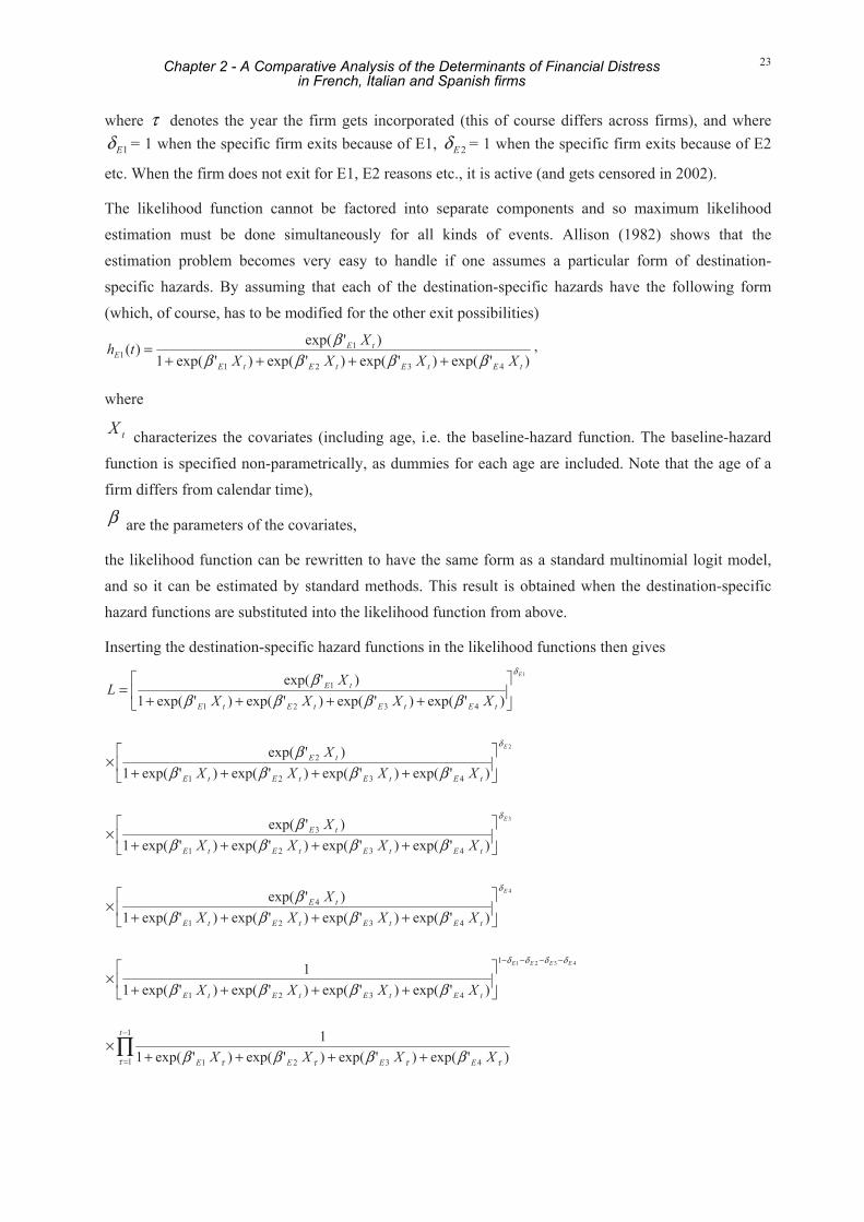
23

where τ denotes the year the firm gets incorporated (this of course differs across firms), and where

1Eδ = 1 when the specific firm exits because of E1, 2Eδ = 1 when the specific firm exits because of E2

etc. When the firm does not exit for E1, E2 reasons etc., it is active (and gets censored in 2002).

The likelihood function cannot be factored into separate components and so maximum likelihood estimation must be done simultaneously for all kinds of events. Allison (1982) shows that the estimation problem becomes very easy to handle if one assumes a particular form of destination-specific hazards. By assuming that each of the destination-specific hazards have the following form (which, of course, has to be modified for the other exit possibilities)

)'exp()'exp()'exp()'exp(1)'exp()(

4321

11

tEtEtEtE

tEE XXXX

Xthββββ

β++++

= ,

where

tX characterizes the covariates (including age, i.e. the baseline-hazard function. The baseline-hazard

function is specified non-parametrically, as dummies for each age are included. Note that the age of a firm differs from calendar time),

β are the parameters of the covariates,

the likelihood function can be rewritten to have the same form as a standard multinomial logit model, and so it can be estimated by standard methods. This result is obtained when the destination-specific hazard functions are substituted into the likelihood function from above.

Inserting the destination-specific hazard functions in the likelihood functions then gives

∏−

=

−−−−

++++×

⎥⎦

⎤⎢⎣

⎡++++

×

⎥⎦

⎤⎢⎣

⎡++++

×

⎥⎦

⎤⎢⎣

⎡++++

×

⎥⎦

⎤⎢⎣

⎡++++

×

⎥⎦

⎤⎢⎣

⎡++++

=

1

1 4321

1

4321

4321

4

4321

3

4321

2

4321

1

)'exp()'exp()'exp()'exp(11

)'exp()'exp()'exp()'exp(11

)'exp()'exp()'exp()'exp(1)'exp(




4321

4

3

2

1

t

EEEE

tEtEtEtE

tEtEtEtE

tE

tEtEtEtE

tE

tEtEtEtE

tE

tEtEtEtE

tE

XXXX

XXXX

XXXXX

XXXXX

XXXXX

XXXXX

L

EEEE

E

E

E

E

τ ττττ

δδδδ

δ

δ

δ

δ

ββββ

ββββ

βββββ

βββββ

βββββ

βββββ


24

which is exactly the same as the likelihood function for the multinomial logit model. The estimation problem can therefore easily be estimated. Active firms are chosen as the reference category. Left truncation and right censoring is handled as in Jenkins (1995), Henley (1998:418) and Rommer (2005).

The coefficients that are reported from the estimation of the problem must be interpreted as contrasts between pairs of categories. As the focus in this study is on finding the effects of the E1 firms, the relevant equation to analyse is the E1 hazard:

tEactive

E Xhh

11 ')log( β=

The interpretation of the equation is that if, for example, the parameter estimate on the solvency ratio is -1.5832, then each 1-level increase in the variable multiplies the odds of moving into financial distress versus staying active by about 0.21 (= exp(-1.5832)).

This above equation is obtained for France, Italy and Spain. In section 5 the parameter estimates are compared and discussed.

Note that from the estimations one also obtains the parameter estimates for the other exits stemming from the following equations:

tEactive

E Xhh

22 ')log( β=

tEactive

E Xhh

33 ')log( β=

tEactive

E Xhh

44 ')log( β=

These results are reported in section 15 (appendix), however, as they are not the focus of this paper, there are not discussed and interpreted.

As a last point, note that unobserved heterogeneity is not allowed for in the estimation problem. This means that if two firms have identical values on the covariates, they also have identical hazard functions, or, in other words, all differences between firms are assumed to be captured using observed explanatory variables. Proxy variables as well as a flexible baseline-hazard specification are used in the estimations. This should mitigate the effects of unobserved heterogeneity, c.f. the discussion Jenkins (2003:102).

5. Results: The Country Models

5.1 Parameter Estimates

Section 15 (appendix) presents the parameter estimates on the E1, E2, E3 and E4 hazard in the three countries. The expected sign and the estimated signs and the significance levels of the E1 hazards are


25

summarized in table 5.1.a (core variables) and table 5.1.b (proxies). Table 6.1 in section 6.1 depicts the parameter estimates of the E1 hazards in the three countries as well as in the pooled model.

Table 5.1.a: Core variables Expected sign Estimated sign Variable

Italy France Spain Italy France Spain

Profitability: Earnings ratio - - - - - -

Solvency: Solvency ratio - - - - - -

Leverage: Loans ratio + + + Insign. + +

Firms size: Log(total assets) - - - + - Insign.

Age - - - - + Insign.

Note: Expected sign: - denotes that the variable is expected to affect financial distress negatively. + denotes that the variable is expected to affect financial distress positively. ? denotes that no certain effect is expected. Estimated sign: - denotes that the variable does affect financial distress negatively. + denotes that the variable does affect financial distress positively. Insign. denotes that the variable is insignificant in the estimations. A significance level of 5 pct. is chosen. Year dummies and sector affiliation dummies were included. Because the data was too sparse otherwise in some countries, a grouping of the sector affiliation dummies took place. France: None of the age dummies were significant in the first estimations. In the final estimations no age dummies are included, only the variable age. Italy and Spain: In the first estimations a flexible baseline-hazard function was specified. This led to a quasi-complete separation of data points, meaning that a maximum likelihood estimate may not be possible to obtain, as the data is too sparse. The consequence of this was to use age in the estimations.

Table 5.1.b: Proxies Expected sign Estimated sign Variable

Italy France Spain Italy France Spain

Subsidiaries: The number of subsidiaries that a company has

registered

? ? ? Insign. Insign. Insign.

Legal form: The effect of being a private limited liability

company

+ + + + Insign. Insign.

Shareholders: The number of recorded shareholders ? ? ? Insign. Insign. Insign.

Ownership variables:

Bvd_indep_a

Bvd_indep_b

Bvd_indep_c

?

?

-

?

?

-

?

?

-

Insign.

Insign.

Insign.

Insign.

Insign.

-

Insign.

Insign.

Insign.

Note: For further details see the note to table 5.1.a.


26

The tables show that there are some similarities across countries, but also that there are quite a lot of differences between the countries. The determinants of financial distress that behaves similarly across countries are 2 of the core variables, namely the earnings ratio and the solvency ratio (they are significant and have a negative sign in all countries, indicating that the higher these ratios are, the less likely a firm is to enter financial distress), and 4 of the proxy variables, namely the number of subsidiaries and shareholders, the ownership variables bvd_indep_a and bvd_indep_b (they are insignificant in all countries).

The variables, which differ between the countries in terms of whether or not they are significant or what sign they have, are the loans to total assets ratio, size, age, legal form and bvd_indep_c.

Loans to total assets were assumed to have a positive coefficient. The parameter estimate is significant and has a positive sign in the French and the Spanish case. The variable is insignificant in the Italian credit-scoring model. A reason for this could be that in comparison with French and Spanish firms, Italian firms fund themselves to a greater extent through trade creditors, c.f. European Committee of Central Balance Sheet Offices (2000:20). Another explanation, which is not mutually exclusive with the first explanation, could be that despite the common feature of "multi-banking" (i.e. firms maintain relations with a number of banks) in all countries, the use of multiple credit lines has become especially large in Italy, c.f. European Committee of Central Balance Sheet Offices (2000:36).25 According to the European Committee of Central Balance Sheet Offices (2000:36f), in Italy, "… the bank bases its lending decisions on real or personal guarantees enabling it to keep its risk exposure within acceptable limits. Moreover, it is much easier and quicker to assess guarantees than to evaluate the company: in the first case, all one needs to do is to evaluate a specific asset (property or financial) and the quality of a surety signatory, making it easier from an administrative viewpoint to provide the specific economic-legal professional training and to process the loan application. The bank therefore bases its lending policy on three closely-related components: spreading the risk by limiting the amount of credit granted to each customer; lending using technical methods allowing for the immediate revocation of the loan application; and the existence of guarantees or surety to cover losses arising from insolvency. This model, which has developed in Italy partly due to a legal framework for insolvency and bankruptcy that systematically gives priority to secured creditors ahead of other categories, limits the bankruptcy risk borne by banks."

Age and size were hypothesized to affect the firms in financial distress negatively. The estimations show that these variables are insignificant in the Spanish case, but significant in the Italian and French case. As mentioned in section 3.2 the size and the age variables are correlated, and so it can be difficult to disentangle the effects. This is what is seen from the estimations. In France and Italy both variables

25 The phenomenon of "multi-banking" is described in European Committee of Central Balance Sheet Offices (2000:36): "A

firm … obtains financing by placing banks in competition with each other to obtain the most favourable contractual terms regarding interest rates, services and maturities. The bank spreads its risks by having smaller commitments and can recover its money inasmuch as the firm can take another loan from another bank".


27

are significant, but with changing signs so that if age is significant and has a positive effect in one country, then size is significant and has a negative effect in the same country, or vice versa. In the French case age affects the likelihood of entering financial distress positively, and size affects the likelihood of entering financial distress negatively. The least significant variable is age. If age is left out of the estimations, size is significant and has a negative sign. In the Italian case the least significant variable of age and size is size. If size is left out of the estimations, then age is negative and significant.

The legal form dummy is constructed such that for all countries, the dummy is equal to one, when the legal form of the company is a private limited liability company. The legal form variable was hypothesized to have a positive sign. The results show that the variable is only significant in the Italian case, where it does have the hypothesized positive sign. The level of share capital between public and private limited liability companies differs between the countries. In Italy the difference in share capital between the two types of legal forms is 110,000 euro, in Spain it is 60,000 euro and in France it is 37,000 euro26. As only firms with 10 employees and a balance sheet of at least 2 million euro are considered in the estimations (c.f. section 3.3), it is not surprising that only an effect of the private limited liability variable for the Italian firms, for which the difference in share capital between the private and public limited liability companies is the largest, is significant.

Ownership information is also included in the estimations. The hypothesis is that the bvd_indep_c has a negative sign. The estimations show that there is no effect for the Italian and Spanish firms and that the parameter estimate is significant for the French firms and it has a negative sign. The reason for this result could be that the French firms are by far the most concentrated firms, c.f. the descriptive statistics in section 13 (appendix).

26 This argument does not take the few French firms in the sample that are listed into account. Different rules apply to the

different countries concerning the amount of share capital that the firms need to hold. In Spain, public limited liability companies need to hold the minimum share capital of around 60,000 euro, whereas private limited liability companies do not need to hold minimum share capital (Information is provided by Informa S.A. in October 2004. Informa S.A. provides Spanish data to Amadeus). In Italy, public limited liability companies need to hold at least 120,000 euro as share capital, and private limited liability companies need to hold at least 10,000 euro (These new rules came into force in January 2004, c.f. Cappiello and Marano (2003:3). Before then public limited liability companies needed to hold 100,000 euro and private limited liability companies needed to hold 10,000 euro, c.f. European Commission (2003b:6)). In France, public limited liability companies need to hold 37,000 euro as share capital (except the ones that are listed on a stock exchange), whereas limited liability companies do not need to hold any share capital (The information on the French firms is as of November 2004. Public limited liability companies: “Société anonyme à conseil d’administration” needs to hold 37,000 euro as share capital. If they are listed on a stock exchange, called “appel public à l’épargne”, they need to hold at least 225,000 euro. (Broadly, “appel public à l’épargne” corresponds to being listed on a stock exchange. However, it is not exactly the same, as “appel public à l’épargne” is a broader concept. It means “selling shares to the public”). “Société anonyme à directoire” need to hold 37,000 euro as share capital. They distinguish themselves from “société anonyme à conseil d’administration” in the way they are governed. “Société par actions simplifiée” need to hold 37,000 euro as share capital. They do not have the possibility of “appel public à l’épargne”. Private limited liability companies: As of August 1st, 2003, “Société à responsabilité limitée” do not need to hold any share capital. Before August 1st, 2003, they needed to hold a minimum of 7,500 euro as share capital).


28

5.2 Discriminatory Power

A measure of how well the models fit the data is the proportion of correct predictions. There is a trade-off between incorrectly classifying a firm that does not exit because of financial distress as a financially distressed firm compared to not classifying a financially distressed firm as financially distressed.

The naïve predictor uses a cut-off value of 0.5, which means that firms that have a predicted probability above 0.5 are classified as financially distressed firms, and that firms that have a predicted probability below 0.5 are classified as active firms. A cut-off level of 0.5 would have seemed reasonable if the samples had entailed 50 per cent financially distressed firms and 50 per cent active firms (or other firms that were not financially distressed). In that case the ratio of financially distressed firms to all other firms would have been exactly 0.5. As the samples sizes here are skewed with only a small fraction of firms in financial distress compared to all other firms in all countries, the 0.5 cut-off is modified. As a cut-off level in the country models the proportion of financially distressed firms used in the estimations to all other firms is used.27 Tables 5.2.a, 5.2.b and 5.2.c. and the more detailed tables 15.d, 15.e and 15.f in section 15 (appendix) show the number of correct predictions, the number of correctly called non-events, as well as the number of type I errors (missing prediction) and type II errors (wrong signal) in the three countries. With the used cut-off levels the models correctly classify between 75 and 88 per cent of the financially distressed firms as financially distressed, and they correctly classify between 68 and 72 per cent of the active firms as active. Had one chosen to use a lower cut-off level, one would have predicted more firms to be financially distressed, but this would be at the cost of an increased number of type 2 errors (wrong signal). If the cut-off level is increased, one would make less type 2 errors, but that would be at the cost of a decreased number of firms that are predicted to be in financial distress (and an increase in the type 1 errors).

The policy maker or the credit institution that uses the model has to make the decision on what cut-off level to use. The cut-off level depends on the “agents” objective function, also called the loss function. It should reflect an assessment of the cost of making type I and type II errors, respectively. The loss-function is discussed in a number of papers in the literature on predicting financial crisis, see for example Demirguc-Kunt and Detragiache (1999) and Bussiere and Fratzscher (2002).

27 This means that in the 1) French case, the cut-off level is 0.01594 (=1703/106830), in the 2) Spanish case, the cut-off level is

0.00238 (=180/75686) and in the 3) Italian case, the cut-off level is 0.00159 (=155/97577).


29

Table 5.2.a: Competing-risks model: France Model prediction:

Event (E1 = financial distress)

Model prediction:

Non-event (E2 = merger, E3 = voluntary liquidation, E4 = inactive (no precision) or active firm)

Event (E1 = financial distress) Correct call of event:

75 pct. (1,280 out of 1,703)


25 pct. (423 out of 1,703)


Type 2 error: Wrong signal:

27 pct. (29,347 out of 106,830)


72 pct. (77,213 out of 106,830)

Table 5.2.b: Competing-risks model: Italy Model prediction:


Model prediction:



88 pct. (137 out of 155)


12 pct. (18 out of 155)



29 pct. (28,283 out of 97,577)

Correct call of non-event

71 pct. (69,294 out of 97,577)

Table 5.2.c: Competing-risks model: Spain Model prediction:


Model prediction:



76 pct. (137 out of 180)


24 pct. (43 out of 180)



32 pct. (24,114 out of 75,686)


68 pct. (51,572 out of 75,686)

6. Results: The Country Models compared with a Pooled Model

The data from the three country models is pooled, and a pooled country model is estimated. The significant variables and their sign, and its predictive ability is compared to the three country models in order to assess the differences in the determinants of financial distress and in the predictive ability of the two model set ups. The results from the specification of the model as a pooled model is interesting in the light of Basel II, which allows for banks to pool their data with other banks in order to overcome their data shortcomings (as valid estimates of the probability of default for individual banks require a


30

considerable amount of data). A number of international data pooling projects have emerged, where banks from various countries pool their data. Because of this development and as, furthermore, many credit institutions in Europe have cross-border activities, the choice between setting up individual country credit-scoring models or a common credit-scoring model is relevant when calculating capital requirements for banks. Therefore, the determinants of corporate failure in French, Italian and Spanish firms are investigated by the estimation of individual country credit-scoring models and a common credit-scoring model. Borup, Kurek and Rommer (2005) take the analysis further and calculate the capital requirements in each country and for the three countries as a whole (i.e. interpreted as one banking portfolio) using different credit-scoring models. The implications for the resulting capital requirements for the portfolio which only entails loans in each country individually and for the three countries as whole (i.e. interpreted as one banking portfolio) are then discussed in their paper. In this paper the focus is not on the resulting capital requirements, but on the factors that drive financial distress. These are discussed using two extreme set ups, namely individual country credit-scoring models and a common credit-scoring model. The common credit-scoring model is estimated using the same explanatory variables as in the country credit-scoring models. It is not extended with either dummies for each country, or with interactions between dummies for each country and some of the already included explanatory variables (e.g. profitability). It has been chosen to show the two extremes, namely the country credit-scoring model and a common credit-scoring model.

6.1 Parameter Estimates

The significance and sign of the parameter estimates in the country models are compared to the significance and sign of the parameter estimates in the pooled model. Table 6.1 shows that all core and proxy variables are significant in the pooled model, except the core variable loans to total assets. This result differs from the results in the country models.

First the core variables are compared in the two model set ups. The country model that resembles the pooled model the most (in terms of what predictors of financial distress are significant and their sign) is the French country model. Except of the loans to total assets ratio, which is not significant in the pooled model, but is significant in the French country model, all core variables are significant in both the French country model and the pooled model and they have the same sign and are of similar size in the two set ups. When the pooled model is compared to the Italian and the Spanish country models, only the earnings ratio and the solvency ratio are significant and have the same sign in both model set ups.

All proxy variables are significant in the pooled model. Only one proxy variable was significant in the French case, none of the proxy variables were significant in the Spanish case and only one proxy variable was significant in the Italian case.


31

Table 6.1: E1 hazard France Spain Italy Pooled model

Age 0.00302* 0.00784 -0.0298* 0.00437*

Size -0.3265* 0.0294 0.2978* -0.3847*

Earnings ratio -1.6054* -1.1842* -2.4314* -1.5114*

Solvency ratio -1.5832* -0.9511* -2.3606* -1.5092*

Loans to total assets 0.3169* 1.4822* -0.2008 0.1227

Legal form 0.0624 0.1166 0.4787* -0.8705*

Shareholders -0.0214 0.0271 0.0258 -0.0775*

Subsidiaries 0.0355 -0.0516 -0.0954 -0.0477*

Bvd_indep_a 0.1973 0.1721 -0.0391 0.8610*

Bvd_indep_b -0.0924 0.0223 -0.2694 0.3020*

Bvd_indep_c -0.3653* -0.3174 0.0127 0.6529*

Note: For details on the country models the reader is referred to table 5.1.a. The pooled country model is estimated using the same variables as in the country models. Again, a significance level of 5 pct. is chosen.

The proxy variables that are significant in the pooled model, but are insignificant in all the country models, are the ownership variables bvd_indep_a and bvd_indep_b and the variables number of shareholders that a firm has registered and number of subsidiaries a firm has registered. Bvd_indep_a and bvd_indep_b are significant and have a positive sign. This indicates that firms whose ownership is not so concentrated are more likely to enter financial distress. The variables number of shareholders that a firm has registered and number of subsidiaries a firm has registered have a negative sign, indicating that a larger number of registered shareholders and subsidiaries lowers the likelihood of financial distress. No hypotheses were set up on the effects of these variables in section 3.2.

The sign of two of the significant proxy variables in the pooled model seem puzzling. This is the sign on the ownership variable bvd_indep_c and the sign on the legal status variable. These variables have different signs compared to the two country models, where they were also significant.

The proxy variable bvd_indep_c is significant and has a negative sign in the French credit-scoring model, indicating that concentration of ownership leads to a lower likelihood of entering financial distress. This result confirms that it is desirable to concentrate ownership among few individual, c.f. Bennedsen and Wolfenzon (2000). It is therefore puzzling that the ownership variable bvd_indep_c is significant and has a positive sign in the pooled model.

The proxy variable legal form is significant and has a negative sign in the Italian credit-scoring model, indicating that private limited liability companies have a larger probability of moving into financial distress. The variable was insignificant for France and Spain. In the pooled model the variable is significant and has a negative sign, indicating that private limited liability companies are less likely to enter financial distress. This is puzzling. One would think that private limited liability companies would


32

be more risky, as they would have less share capital to loose compared with public limited liability companies.

The overall result is that the pooled model delivers parameter estimates, which in terms of significance and sign differ to quite an extent from all the country credit-scoring models. The implication of this is that country credit-scoring should be estimated. It does not make sense to pool the data and estimate a common credit-scoring model.

6.2 Discriminatory Power

Table 6.2.a shows that, overall, the discriminatory power of the pooled country model is very alike the individual country models for France and Spain (and less so for Italy). The pooled country model correctly classifies 74 pct. of the financially distressed firms as financially distressed, and 72 pct. of the active firms as active.28 The overall result of table 6.2.a hides important differences between the two model set ups. Table 6.2.b shows that only 66 pct. (=(34,187+152,218)/282,131)) of the predictions are the same in the two model set ups. In quite a number of cases the country models predict an event, when the pooled country model does not predict an event (49,135) and vice versa.

Table 6.2.a: Competing-risks model for France, Italy and Spain (pooled country model) Model prediction:


Model prediction:



74 pct. (1,498 out of 2,038)


26 pct. (540 out of 2,038)



28 pct. (79,280 out of 280,093)


72 pct. (198,131 out of 280,093)

Table 6.2.b: A comparison of the predictions of the three country models and the pooled country model Pooled country model

Model prediction: Event Model prediction: Non-event Sum

Model prediction: Event 34,187 49,135 83,322 Country models

Model prediction: Non-event 46,591 152,218 198,809

Sum 80,778 201,353 282,131

28 The cut-off level is 0.00728 (=2038/280093).


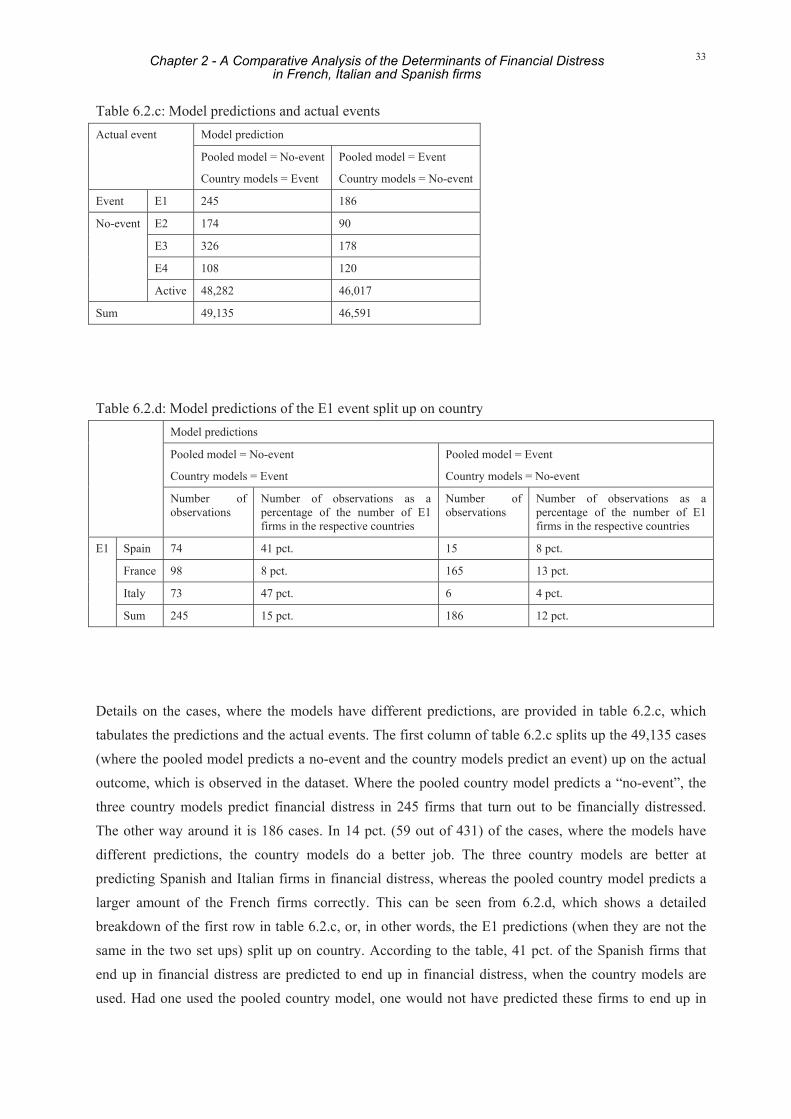
33

Table 6.2.c: Model predictions and actual events Model prediction Actual event

Pooled model = No-event

Country models = Event

Pooled model = Event

Country models = No-event

Event E1 245 186

E2 174 90

E3 326 178

E4 108 120

No-event

Active 48,282 46,017

Sum 49,135 46,591

Table 6.2.d: Model predictions of the E1 event split up on country Model predictions

Pooled model = No-event

Country models = Event

Pooled model = Event

Country models = No-event


Number of observations as a percentage of the number of E1 firms in the respective countries


Number of observations as a percentage of the number of E1 firms in the respective countries

Spain 74 41 pct. 15 8 pct.

France 98 8 pct. 165 13 pct.

Italy 73 47 pct. 6 4 pct.

E1

Sum 245 15 pct. 186 12 pct.

Details on the cases, where the models have different predictions, are provided in table 6.2.c, which tabulates the predictions and the actual events. The first column of table 6.2.c splits up the 49,135 cases (where the pooled model predicts a no-event and the country models predict an event) up on the actual outcome, which is observed in the dataset. Where the pooled country model predicts a “no-event”, the three country models predict financial distress in 245 firms that turn out to be financially distressed. The other way around it is 186 cases. In 14 pct. (59 out of 431) of the cases, where the models have different predictions, the country models do a better job. The three country models are better at predicting Spanish and Italian firms in financial distress, whereas the pooled country model predicts a larger amount of the French firms correctly. This can be seen from 6.2.d, which shows a detailed breakdown of the first row in table 6.2.c, or, in other words, the E1 predictions (when they are not the same in the two set ups) split up on country. According to the table, 41 pct. of the Spanish firms that end up in financial distress are predicted to end up in financial distress, when the country models are used. Had one used the pooled country model, one would not have predicted these firms to end up in


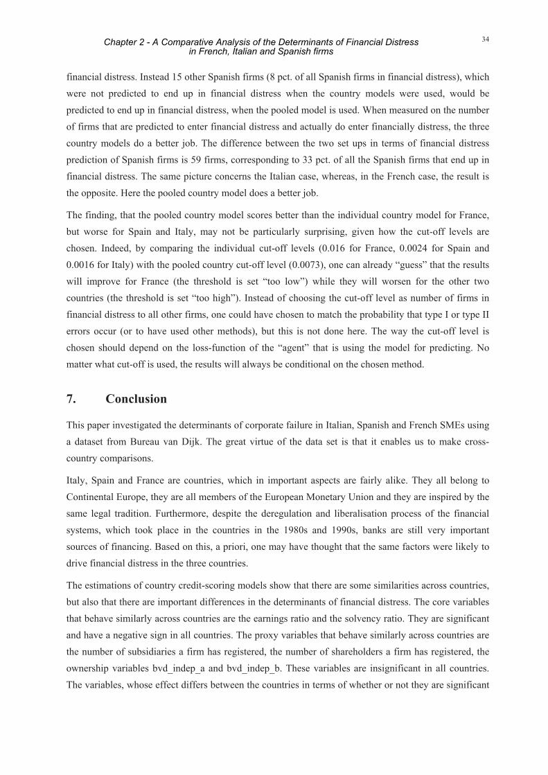
34

financial distress. Instead 15 other Spanish firms (8 pct. of all Spanish firms in financial distress), which were not predicted to end up in financial distress when the country models were used, would be predicted to end up in financial distress, when the pooled model is used. When measured on the number of firms that are predicted to enter financial distress and actually do enter financially distress, the three country models do a better job. The difference between the two set ups in terms of financial distress prediction of Spanish firms is 59 firms, corresponding to 33 pct. of all the Spanish firms that end up in financial distress. The same picture concerns the Italian case, whereas, in the French case, the result is the opposite. Here the pooled country model does a better job.

The finding, that the pooled country model scores better than the individual country model for France, but worse for Spain and Italy, may not be particularly surprising, given how the cut-off levels are chosen. Indeed, by comparing the individual cut-off levels (0.016 for France, 0.0024 for Spain and 0.0016 for Italy) with the pooled country cut-off level (0.0073), one can already “guess” that the results will improve for France (the threshold is set “too low”) while they will worsen for the other two countries (the threshold is set “too high”). Instead of choosing the cut-off level as number of firms in financial distress to all other firms, one could have chosen to match the probability that type I or type II errors occur (or to have used other methods), but this is not done here. The way the cut-off level is chosen should depend on the loss-function of the “agent” that is using the model for predicting. No matter what cut-off is used, the results will always be conditional on the chosen method.

7. Conclusion

This paper investigated the determinants of corporate failure in Italian, Spanish and French SMEs using a dataset from Bureau van Dijk. The great virtue of the data set is that it enables us to make cross-country comparisons.

Italy, Spain and France are countries, which in important aspects are fairly alike. They all belong to Continental Europe, they are all members of the European Monetary Union and they are inspired by the same legal tradition. Furthermore, despite the deregulation and liberalisation process of the financial systems, which took place in the countries in the 1980s and 1990s, banks are still very important sources of financing. Based on this, a priori, one may have thought that the same factors were likely to drive financial distress in the three countries.

The estimations of country credit-scoring models show that there are some similarities across countries, but also that there are important differences in the determinants of financial distress. The core variables that behave similarly across countries are the earnings ratio and the solvency ratio. They are significant and have a negative sign in all countries. The proxy variables that behave similarly across countries are the number of subsidiaries a firm has registered, the number of shareholders a firm has registered, the ownership variables bvd_indep_a and bvd_indep_b. These variables are insignificant in all countries. The variables, whose effect differs between the countries in terms of whether or not they are significant


35

or what sign they have, are the loans to total assets ratio, size, age, legal form and the ownership variable bvd_indep_c.

The data from the three country models is pooled, and a common model is estimated. The significant variables and their sign, and the predictive ability of the common credit-scoring model is compared to the three country models in order to assess the differences in the determinants of financial distress and in the predictive ability of the two model set ups. The results from the individual credit-scoring models are confirmed by the estimation of the pooled model, which shows that the pooled model delivers parameter estimates that differ to quite an extent from all the country credit-scoring models. The comparison of the core variables in the pooled model with the individual country models show that the country that resembles the pooled model the most (in terms of what predictors of financial distress are significant and their sign) is France. The comparison of the proxy variables in the pooled model with the individual country models showed that there were no similarities between the country models and the pooled model. The overall conclusion is that the pooled model delivers parameter estimates that differ to quite an extent from the all the country credit-scoring models. A comparison of the predictive ability of the pooled model and the country models hides important differences between the two model set ups, namely that the pooled model does better for France than the French credit-scoring model, but worse for Spain and Italy than the Spanish and the Italian credit-scoring models. It can seem a bit surprising that the French country model performs worse for France than the pooled country model, but it is not so surprising, when one takes a closer look on how the cut-off levels are chosen. It is therefore important to highlight that the result is conditional on the chosen cut-off levels. It was chosen to use the proportion of firms in financial distress to all other firms.

The overall conclusion from the analysis is that not even in this case, where the analysed sample of countries is fairly homogenous, does it make sense to estimate one common credit-scoring model. This is an important conclusion, which has implications for at least two policy areas, namely financial stability analysis and Basel II.


36

8. LITERATURE

Alderman, H., J. R. Behrman, H-P. Kohler, K. A. Maluccio and S. C. Watkins, 2000. Attrition in Longitudinal Household Survey Data. Some Tests for Three Developing-Country Samples. Policy Research Working Paper no. 2447, The World Bank, September 2000.

Allison, P. D., 1982. Discrete-time Methods for the Analysis of Event Histories. In Samuel Leinhardt (ed.), Sociological Methodology 1982, San Francisco: Jossey-Bass, pp. 61-98



Altman, E. I., G. Marco and F. Varetto, 1994. Corporate distress diagnosis: Comparisons using linear discriminant analysis and neural networks (the Italian experience). Journal of Banking and Finance, vol. 18., pp. 505-529

Ayadi, R., 2004. Impact of the New Basel Capital Accord on SME Financing. In The New Basel Capital Accord and the Future of the European Financial System, Report of a CEPS Task Force no. 51, Rapporteurs: R. Ayadi and A. Resti, April 2004

Bardos, M., 1998. Detecting the risk of company failure at the Banque de France. Journal of Banking & Finance, vol. 22, pp. 1405-1419


Basel Committee on Banking Supervision, 2004. International Convergence of Capital Measurement and Capital Standards. A Revised Framework. Bank for International Settlements, June 2004


Bennedsen, M., 2004. The Governance of Closely Held Corporations: Ownership Structure, Family Management and the Role of the Corporate Board. Manuscript presented at the Annual Meeting in Nationaloekonomisk Forening, 2004.

Bennedsen, M. and D. Wolfenzon, 2000. The balance of power in closely held corporations. Journal of Financial Economics, vol. 58, pp. 113-139



37


Bunn, P., and V. Redwood, 2003. Company accounts based modelling of business failures and the implications for financial stability. Bank of England Working Paper No. 210

Bureau van Dijk, 2004. Ownership Database. March 2004

Bussiere, M. and M. Fratzscher, 2002. Towards a new early warning system of financial crises. European Central Bank working paper series. Working paper no. 145, May 2002.

Cappiello, S. and G. Marano, 2003. The Reform of the Legal Framework for Italian Enterprises and the 2003 Company Law. International Company and Commercial Law Review, n. 6, 2003

Cifarelle, D. M. and F. Corielli, 1988. Business Failure Analysis. A Baysian Approach With Italian Firm Data. Studies in Banking and Finance, no. 7, pp. 73 - 89

Corcóstegui, C., L. González-Mosquera, A. Marcelo and C. Trucharte, 2003. Analysis of procyclical effects on capital requirements derived from a rating system. Paper presented at Basel Committee/Banca d’Italia workshop, 20-21 March 2003.

Creditreform, 2002. Insolvencies in Europe 2001/2. A Survey by the Creditreform Economic Research Unit

Creditreform, 2003. Insolvencies in Europe 2002/3. A Survey by the Creditreform Economic Research Unit

Danmarks Statistik, 2002. Rapport fra projektgruppen om Demografi. Danmarks Statistik, Erhvervsstruktur, December 2002.

Demirguc-Kunt, A. and E. Detragiache, 1999. Monitoring Banking Sector Fragility: A Multivariate Logit Approach. International Monetary Fund Working Paper, WP/99/

Davydenko, S. A. and J. R. Franks, 2004. Do bankruptcy codes matter? A study of defaults in France, Germany, and the UK. Unpublished manuscript, June 2004.

Dietsch, M. and J. Petey, 2002. The credit risk SME loans portfolios: Modeling issues, pricing, and capital requirements. Journal of Banking & Finance, vol. 26, pp. 303-322

Diggle, P. and M. G. Kenward, 2004. Informative Drop-out in Longitudinal Data Analysis. Applied Statistics, vol. 43, no. 1, pp. 49-93

Dyrberg, A., 2004. Firms in Financial Distress: An Exploratory Analysis. Working paper no. 17, Danmarks Nationalbank

European Central Bank, 2002. Report on Financial Structures. European Central Bank

European Central Bank, 2004. Financial Stability Review, December 2004. European Central Bank


38

European Commission, 2003a. Bankruptcy and a fresh start: stigma on failure and legal consequences of bankruptcy. November 2003

European Commission, 2003b. Bankruptcy and a fresh start: stigma on failure and legal consequences of bankruptcy. Italian Country Study. November 2003

European Commission, 2003c. Bankruptcy and a fresh start: stigma on failure and legal consequences of bankruptcy. Spanish Country Study. November 2003

European Commission, 2003d. Bankruptcy and a fresh start: stigma on failure and legal consequences of bankruptcy. French Country Study. November 2003

European Commission, 2003e. Commission Recommendation of 6 May 2003 concerning the definition of micro, small and medium-sized enterprises. Official Journal of the European Union, L 124/36, 2003

European Committee of Central Balance Sheet Offices (2000), Corporate Finance in Europe from 1986 to 1996. Own Funds Working Group, European Committee of Central Balance Sheet Offices, 2000.

Eurostat, 2004. Business Demography. Recommendations Manual. Eurostat, 2004

Feelders, A. J., 2003. An Overview of Model Based Reject Inference for Credit Scoring. Unpublished manuscript

Fernandez, A. I, 1988. A Spanish Model for Credit Risk Classification. Studies in Banking and Finance, vol. 7, pp. 115-125

Fitzgerald, J., P. Gottschalk and R. Moffitt, 1998. An Analysis of Sample Attrition in Panel Data. The Journal of Human Resources, vol. 33, no. 2, pp. 251-299

Fitzmaurice, G. M., A. F. Heath and P. Clifford, 1996. Logistic Regression Models for Binary Panel Data with Attrition. Journal of the Royal Statistical Society. Series A (Statistics in Society), vol. 159, no. 2, pp. 249-263



Hayden, E., 2003. Are Credit Scoring Models Sensitive With Respect to Default Definitions? Evidence from the Austrian Market. Unpublished manuscript, 2003

Henley, A., 1998. Residential mobility, housing equity and the labour market. The Economic Journal, 108, pp. 414-427

Hermalin, B. E. and M. S. Weisbach, 2003. Boards of Directors as an Endogenously Determined Institution: A Survey of the Economic Literature. FRBNY Economic Policy Review, April 2003.


39

Hunter, J. and N. Isachenkova, 2000. Failure Risk: a Comparative Study of UK and Russian Firms. Department of Economics and Finance Brunel University, Discussion Paper 00-1



Jiménez, G. and J. Saurina, 2004. Collateral, type of lender and relationship banking as determinants of credit risk. WP no. 0414, Banco de España


Lando, D., 2004. Credit Risk Modeling. Theory and Applications. Princeton Series in Finance

La Porta, R., F. Lopez-De-Silanes, A. Shleifer and R. Vishny, 1998. Law and Finance. The Journal of Political Economy, vol. 106, no. 6, pp. 1113-1155

Memorandum of Understanding on the exchange of information among national credit registers for the purpose of passing it on to reporting institutions, 20 February 2003

Moody’s Investors Service, 2000. Moody’s RiskCalc For Private Companies: Moody’s Default Model. Rating Methodology, May 2000

Moody’s Investors Service, 2001a. Moody’s RiskCalc For Private Companies: Spain. Rating Methodology, July 2001

Moody’s Investors Service 2001b. Moody’s RiskCalc For Private Companies: France. Rating Methodology, December 2001

Moody’s Investors Service 2002. Moody’s RiskCalc For Private Companies: Italy. Rating Methodology, October 2002


Ooghe, H. and S. Balcaen, 2002. Are failure prediction models transferable from one country to another? An empirical study using Belgian financial statements. Vlerick Working Papers 2002/5


Rommer, A. D. Testing the Assumptions of Credit-scoring Models. Working Paper no. 28, Danmarks Nationalbank

Scheule, H., 2003. Prognose von Kreditausfallrisiken. Dissertation zur Erlangung des Grades eines Doktors der Wirtschaftswissenshcaften eingereicht an der Wirtschaftswissenschartlichen Fakultät der Universität Regensburg, vorgelegt von Harald Scheule, Schongau, April 2003


40





41

9. Appendix: Other Studies

Table 9.a: Studies using French data Study Data Method Default definition

Bardos (2001)

(see also Bardos (1998))

FR

The Banque de France FIBEN database (The database is almost exhaustive for firms with a turnover exceeding FRF 5 million. Some smaller firms are recorded in the database, particularly if their debt exceeds FRF 2.5 million. The debt of the firms in the database is proportionally higher than that seen in the exhaustive population surveyed by INSEE (French Institute of Statistics and Economics Studies)). The study uses representative data on French companies in the FIBEN database, which have a turnover exceeding EUR 0.75 million or whose bank loans exceeded (five times) a risk declaration threshold.

Period: 1991 – 2000

Probability of default (PD) estimation: Score (discriminant analysis). A probability of failure is associated with each value of the score

Failure = opening of legal proceedings. It is noted that the opening of legal proceedings mainly concerns small- and medium-sized companies rather than large companies, as large companies, which are experiencing difficulties, rarely submit their balance sheet to the registrars of Commercial Courts (they generally restructure and/or negotiate their debts)

Dietsch and Petey (2002)

FR

The analysis is done on 224.000 French SMEs. Data is provided by Coface SCRL.

Period: 1995 –1999

PD estimation: Ordered probit model and a model using a gamma distribution.

Default corresponds to bankruptcy

Moody’s Investors Service (2001b)

FR

1,323,754 financial statements and 25,229 defaults from 253,268 French private companies. Only firms with a turnover of at least 0.5 million euro.

Period: 1990 – 1999

PD estimation:

Binomial logit model

Bankruptcy or insolvency

This paper

ES

FR

IT

Italy: 97,733 SME firm-years

Spain: 75,866 SME firm-years

France: 108,533 SME firm-years

Data is provided by Bureau van Dijk (Amadeus database).

Period covered for all countries: 2000 – 2002

PD estimation:

Competing-risks model

Financially distressed firms include firms that are bankrupt, active (receivership) and active (default of payments)


42

Table 9.b: Studies using Spanish data Study Data Method Default definition

Jiménez and Saurina (2004)

ES

Credit Register of the Bank of Spain (CIR). Monthly information on all loans granted by credit institutions in Spain for a value of 6,000 euros. The data has been subjected to various filters, e.g. only loans to companies above a threshold of 24,000 euros are used. Data on over 3 million loans are analysed.

Data from December. Five years are included: 1987, 1990, 1993, 1997, 2000

Probability of default (PD) estimation: Binomial logit model

Default on payment is considered to have occurred when, three months after the date of maturity, the debt balance remains unpaid or when there are reasonable doubts as to its repayment

Corcóstegui, González-Mosquera, Marcelo and Trucharte (2003)

ES

Credit Register of the Bank of Spain (CIR). Bank of Spain’s Central Financial Database (CBBE). Private database SABE. The raw data consists of the obligors that are found in all three databases. Various filters are used, including a minimum size threshold in terms of annual volume of sales equal to 9 million euro. 73,321 obligors are analysed.

Period: 1993 – 2000

PD estimation: Binomial logit model

Default on payment is considered to have occurred when, three months after the date of maturity, the debt balance remains unpaid or when there are reasonable doubts as to its repayment

Fernandez (1988)

ES

A matched sample of 70 firms. Data set was drawn from the files of loan clients of a Spanish bank.

PD estimation: Univariate analysis, factor analysis by principal components, discriminant analysis

Failure is defined as credit applicants that the bank classified as insolvent (e.g. operations whose ability to repay a loan is doubtful, and thus, not only firms which have failed in a legal sense (bankrupt firms))

Moody’s Investors Service (2001a)

ES

569,181 financial statements and 2,265 defaults from 140,790 companies. Only firms with a turnover of at least 0.5 million euro. The database is developed by Equifax.

Period: 1992 – 1999

PD estimation:


Bankruptcy or insolvency

This paper

ES

FR

IT






PD estimation:




43

Table 9.c: Studies using Italian data Study Data Method Default definition

Cifarelli and Corielli (1988)

IT

A sample of 27 unsound and 196 sound firms is used (reference is taking in a ‘major’ Italian bank)

Probability of default (PD) estimation:

A bayesian variant to discriminant analysis

Default corresponds to bankruptcy

Altman, Marco and Varetto (1994)

IT

A matched sample of all together 1,000 healthy and unsound industrial Italian firms. Focus is on medium and small sized businesses. For this reason, companies with sales of more than 100 billion lira (i.e. 60 million dollars) have been excluded from the sample. The sample is obtained from the Central dei Bilanci (CB), which is an organization established by the Banca d’Italia.

Period: 1982 – 1992

PD estimation:

Linear discriminant analysis, logit analysis and neural networks

Defaults correspond to 1) bankruptcy, 2) firms that are wound up in temporary receivership, 3) firms that had stated they were in dire straits with regard to their payments to the banks.

Moody’s Investors Service (2002)

IT

124,937 financial statements and 958 defaults from over 52,329 Italian private companies. Only firms with a turnover of at least 0.5 million euro.

Period: 1995 – 1999

PD estimation:


Defaults are based on three sources of information 1) Sponsor bank experience, 2) provisioning data and 3) insolvency statistics

This paper

ES

FR

IT






PD estimation:




44

10. Appendix: Legal status codes

Table 10.a: French legal status codes Situation normale, avec comptes Active

Pas d'obligation de dépôt (NC) Active

Plan de continuation (PC) Active (receivership)

Redressement judiciaire par jugement (RJ) Active (receivership)

Liquidation par jugement (LJ) Bankruptcy

Absorption, fusion ou rachat (AF) Dissolved (merger)

Liquidation à l'amiable (LA) In liquidation

Cessation d'activité (CE) Inactive (no precision)

Cessation de paiement (CP) Active (default of payments)

Source: Bureau van Dijk

Table 10.b: Italian legal status codes Ditta attiva Active

Ditta in liquidazione In liquidation

Ditta in fallimento Bankruptcy

Ditta sospesa Active (dormant)

Ditta inattiva Inactive (no precision)

Ditta cassata Dissolved

Ditta cessata per trasferimento Dissolved (merger)


Table 10.c: Spanish legal status codes Activa Active

Suspension de pagos Active (default of payments)

Quiebra Bankruptcy

Disuelta Dissolved

Absorbida Dissolved (merger)

Extinguida Dissolved

Inactiva Inactive (no precision)



45

11. Appendix: Sample Selection in Details

The raw data is split up according to 6 different codes: C1 = Consolidated statement with no unconsolidated companion, C2 = Consolidated statement with an unconsolidated companion, U1 = Unconsolidated statement with no consolidated companion, U2 = Unconsolidated statement with a consolidated companion, LF = Limited financial data, probably unconsolidated, N.A. = No financial data available. In order to avoid double accounting, only companies with the codes U1 and U2 are analysed (For Italy, Spain and France there are no financial statements with the LF code). In the raw data there are 3,777,275 firm-year observations covering the period 2000 – 2002 (FR: 2,135,745, IT: 461,985, ES: 1,179,545).

After the exclusion of financial institutions and non-financial holding companies, there are 3,629,353 firm-year observations left (FR: 2,019,361, IT: 459,611, ES: 1,150,381).

A panel dataset is constructed. If a company hands in two financial statements, only the last financial statement is included in the estimations (FR: 2,019,216, IT: 459,577, ES: 1,154,378). Active companies are excluded if they hand in a financial statement in 2000 and 2002 (and not in 2001) (FR: 1,992,780, IT: 442,608, ES: 1,153,092).

The first year a specific company enters the dataset, it is ensured that it has at least 10 employees and total assets equal to or above 2 million euro. Remaining are 383,845 firm-year observations (FR: 137,183, IT: 146,360, ES: 100,302). Companies with 250 employees or more and companies with a total balance sheet of more than 43 million euro are excluded, making the database a total of 345,078 firm-year observations (FR: 120,758, IT: 135,010, ES: 89,310).

Finally, various corrections are made to the database (e.g. firms with illogical variables, such as short-term debt less than zero and a solvency ratio larger than 100 pct., are excluded) (FR: 118,395, IT: 134,038, ES: 81,162).

Only public limited liabilities and private limited liabilities are analysed. (FR: 113,421, IT: 126,056, ES: 80,175).

Firms with missing variables on any of the explanatory variables are excluded. Remaining are 299,746 firm-year observations (FR: 113,420, IT29 30: 106,166, ES: 80,160).

The attritioners are excluded making the database a total of 282,131 firm-year observations (FR: 108,533, IT: 97,732, ES: 75,866).

29 Most of the Italian firms are excluded because there is no information on the incorporation date (and so the age of the

company cannot be constructed). 30 BvD has provided me with further information in the Italian firms. As of 2002, their Italian data provider includes

information on firms with a turnover between 500.000 and 1.000.000 euro (these firms were not included before). In the dataset 927 of the Italian firms are new firms in 2002 with a turnover less than 1.000.000 euro.


46

12. Appendix: Detailed analysis of the Attritioners

12.1 Introduction

The attritioners are analysed in detail in this appendix. The means of the attritioners and the non-attritioners are compared. To investigate whether the means of various variables are significantly different, t-tests are performed and results are reported. The null hypothesis is that there is no difference between the means. The alternative hypothesis is that they are different. In order for the t-test to be valid, it is necessary that the responses are independent of each other, and the observations should come from a normal distribution. If the sample sizes are equal, the procedure is fairly robust to violations of the normality assumption. Here the sample sizes are not equal, and so the nonparametric Wilcoxon’s test is also performed. The result of this test is very similar to the t-test (results are not reported). The t-test assumes equal variances. A test that allows for non-equal variances is the Satterthwaite test. This test is also performed and results are reported. Thereafter attrition probits are estimated. The variables that drive attrition are discussed. Finally, a robustness check is performed.

12.2 Testing for Equal Means of the Explanatory Variables

France: 2000 sample

The E5 firms and non-E5 firms resemble each other (table 12.2.a). Out of the 22 core, proxy and control variables, which are examined, only 3 – 4 core and proxy variables (depending on the test) and 3 – 4 control variables (depending on the test), are rejected to have equal means using both the t-test and the Satterthwaite test for the 2000 sample. The core variables that are rejected to have equal means are the solvency ratio, age and size (only t-test), and the proxy variable, which is rejected to have equal means, is the dummy legalform. The 4 sector affiliation dummies that are rejected to have equal means are: dumman, dumcon, dummin (only Satterthwaite test) and dumpub.

It is worth noticing that the solvency ratio is larger for the attritioners than for the non-attritioners. The solvency ratio is hypothesized to affect the firm that enter financial distress negatively, and so, based on this variable, there is no sign of the E5 firms being weaker than the non-E5 firms. The age of the E5 firms is lower than the age of the non-E5 firms and the E5 firms are larger than the non-E5 firms. Both age and size were hypothesized to affect firms in financial distress negatively. Private limited liability companies are more likely to be among the E5 firms compared to the non-E5 firms. This variable, which is a proxy for the willingness to take on risk, was hypothesized to affect the firms in financial distress positively.


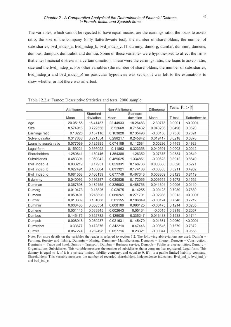
47

The variables, which cannot be rejected to have equal means, are the earnings ratio, the loans to assets ratio, the size of the company (only Satterthwaite test), the number of shareholders, the number of subsidiaries, bvd_indep_a, bvd_indep_b, bvd_indep_c, IT dummy, dumorg, dumfar, dummin, dumene, dumbus, dumpub, dumtrahot and dumtra. Some of these variables were hypothesized to affect the firms that enter financial distress in a certain direction. These were the earnings ratio, the loans to assets ratio, size and the bvd_indep_c. For other variables (the number of shareholders, the number of subsidiaries, bvd_indep_a and bvd_indep_b) no particular hypothesis was set up. It was left to the estimations to show whether or not there was an effect.

Table 12.2.a: France: Descriptive Statistics and tests: 2000 sample

Attritioners Non-Attritioners Difference Tests: t>Pr

Mean Standard deviation Mean

Standard deviation Mean T-test Satterthwaite

Age 20.05155 16.41487 22.44933 18.26483 -2.39778 0.0001 <0.0001 Size 8.574916 0.722556 8.52668 0.715432 0.048236 0.0496 0.0520 Earnings ratio 0.10225 0.157116 0.103828 0.135496 -0.00158 0.7356 0.7691 Solvency ratio 0.317633 0.271554 0.298217 0.245842 0.019417 0.0218 0.0370 Loans to assets ratio 0.077069 0.125895 0.074109 0.112584 0.00296 0.4453 0.4923 Legal form 0.159221 0.366092 0.11863 0.323358 0.040591 0.0003 0.0012 Shareholders 1.280641 1.159446 1.354388 1.26352 -0.07375 0.0884 0.0649 Subsidiaries 0.483391 1.059042 0.489625 1.334851 -0.00623 0.8912 0.8649 Bvd_indep_a 0.033219 0.17931 0.029331 0.168736 0.003888 0.5028 0.5271 Bvd_indep_b 0.027491 0.163604 0.031321 0.174188 -0.00383 0.5211 0.4962 Bvd_indep_c 0.681558 0.466139 0.677749 0.467346 0.003809 0.8123 0.8119 It dummy 0.040092 0.196287 0.030538 0.172066 0.009553 0.1072 0.1552 Dumman 0.367698 0.482455 0.326003 0.468756 0.041694 0.0096 0.0119 Dumorg 0.019473 0.13826 0.02075 0.14255 -0.00128 0.7939 0.7880 Dumcon 0.050401 0.218896 0.080261 0.271701 -0.02986 0.0013 <0.0001 Dumfar 0.010309 0.101068 0.01155 0.106849 -0.00124 0.7348 0.7212 Dummin 0.003436 0.058554 0.008189 0.090125 -0.00475 0.1214 0.0205 Dumene 0.001145 0.033845 0.002643 0.05134 -0.0015 0.3918 0.2057 Dumbus 0.145475 0.352782 0.129038 0.335247 0.016438 0.1538 0.1744 Dumpub 0.008018 0.089237 0.021631 0.145479 -0.01361 0.0060 <0.0001 Dumtrahot 0.33677 0.472876 0.342219 0.47446 -0.00545 0.7379 0.7372 Dumtra 0.057274 0.232498 0.057716 0.23321 -0.00044 0.9559 0.9558 Note: For more details on the variables the reader is referred to section 3.2. The following abbreviations are used: Dumfar = Farming, forestry and fishing, Dummin = Mining, Dumman= Manufacturing, Dumener = Energy, Dumcon = Construction, Dumtraho = Trade and hotel, Dumtra = Transport, Dumbus = Business service, Dumpub = Public service activities, Dumorg = Organisations. Subsidiaries: This variable measures the number of subsidiaries that a company has registered. Legal form: This dummy is equal to 1, if it is a private limited liability company, and equal to 0, if it is a public limited liability company. Shareholders: This variable measures the number of recorded shareholders. Independence indicators: Bvd_ind_a, bvd_ind_b and bvd_ind_c.


48

France: 2001 sample

Using the 2001 sample, out of the 22 core, proxy and control variables it is rejected that 3 core and proxy variables and 2 sector affiliation dummies have equal means, c.f. table 12.2.b. The core and proxy variables, which are rejected to have equal means, are the earnings ratio, the age of a company and the dummy variable legal form. The two sector affiliation dummies, which are rejected to have equal means, are dumcon and dumbus.

E5 firms have an earnings ratio that is smaller than the earnings ratio for the non-E5 firms in the 2001 sample. This could indicate that weak firms are more likely to be among the E5 firms. E5 firms are also younger than the non-E5 firms. As for the 2000 sample, in the 2001 sample private limited liability companies are more likely to be among the E5 firms compared to the non-E5 firms.

The variables, which cannot be rejected to have equal means, are the solvency ratio, the loans to assets ratio, the size of the company, the number of shareholders, the number of subsidiaries, bvd_indep_a, bvd_indep_b, bvd_indep_c, IT dummy, dumman, dumorg, dumfar, dummin, dumene, dumpub, dumtrahot and dumtra. Some of these variables were hypothesized to affect the firms that enter financial distress, e.g. the solvency ratio was hypothesized to have a positive sign and the loans to assets ratio was hypothesized to have a negative sign. No hypothesis was made on the effects of other variables, e.g. the number of shareholders and the number of subsidiaries.

France: Conclusion

In the French case, very few core and proxy variables are found to have different means. In the 2000 sample the mean of the solvency ratio, age, size (only t-test) and legal form was significantly different between E5 firms and non-E5 firms, and in the 2001 sample, the mean of the earnings ratio, age and legal form were significantly different between E5 firms and non-E5 firms. The solvency ratio is higher for E5 firms compared to non-E5 firms (2000 sample). The results in this section indicate that the E5 firms are stronger than the non-E5 firms. At the same time, the earnings ratio was found to be lower for the E5 firms than for the non-E5 firms, indicating that the E5 firms are weaker than the non-E5 firms (2001 sample). Age and size affect financial distress in opposite directions (2000 sample). For the 2001 sample, age of E5 and non-E5 firms cannot be rejected to have equal means with the E5 firms being younger than the non-E5 firms. Both age and size were hypothesized to affect the firms in financial distress negatively. Legal form is rejected to have equal means in both samples. In both samples private limited liability companies are more likely to be among the attritioners.

As most core and proxy variables cannot be rejected to have equal means for E5 and non-E5 firms, and as the effect of the solvency ratio (2000 sample) and the earnings ratio (2001 sample) give conflicting results concerning the potential bias of the estimates, the overall conclusion from the comparisons of means between the French E5 firms and non-E5 firms is that the means of the indicators, which are central to the study, do not differ in a systematically way between E5 firms and non-E5 firms.


49

Table 12.2.b: France: Descriptive Statistics tests: 2001 sample

Attritioners Non-Attritioners Difference Tests: t>Pr


Standard Deviation Mean T-test Satterthwaite test

Age 20.4261 17.54955 22.40174 18.01933 -1.97564 <0.0001 <0.0001

Size 8.477076 0.722979 8.497622 0.734085 -0.02055 0.1763 0.1707 Earnings ratio 0.086599 0.19748 0.098183 0.154471 -0.01158 0.0004 0.0042 Solvency ratio 0.290889 0.29748 0.297292 0.265901 -0.0064 0.2489 0.2958 Loans to assets ratio 0.079453 0.124438 0.075101 0.118124 0.004352 0.0765 0.0905 Legal form 0.1751 0.380129 0.12983 0.336121 0.04527 <0.0001 <0.0001

Shareholders 1.318474 1.185226 1.337381 1.278889 -0.01891 0.4735 0.4438 Subsidiaries 0.465863 1.273963 0.448968 1.240744 0.016896 0.5117 0.5214 Bvd_indep_a 0.03494 0.183664 0.029311 0.168679 0.005629 0.1093 0.1372 Bvd_indep_b 0.032932 0.178494 0.031381 0.174348 0.001551 0.6682 0.6746 Bvd_indep_c 0.664659 0.472204 0.669298 0.470472 -0.00464 0.6342 0.6353 It dummy 0.038153 0.191603 0.033258 0.179312 0.004895 0.1896 0.2158 Dumman 0.314859 0.464553 0.31348 0.463914 0.00138 0.8859 0.8860 Dumorg 0.022892 0.149588 0.021611 0.145411 0.001281 0.6713 0.6789 Dumcon 0.069478 0.254316 0.083711 0.276957 -0.01423 0.0127 0.0073 Dumfar 0.010843 0.103586 0.012034 0.109037 -0.00119 0.5971 0.5805 Dummin 0.006426 0.079919 0.007838 0.088188 -0.00141 0.4368 0.3969 Dumene 0.002811 0.052957 0.002456 0.049502 0.000355 0.7305 0.7454 Dumbus 0.150602 0.357733 0.133915 0.340565 0.016688 0.0184 0.0240 Dumpub 0.018474 0.134684 0.021473 0.144956 -0.003 0.3159 0.2850 Dumtrahot 0.35261 0.477879 0.34544 0.475518 0.00717 0.4669 0.4689 Dumtra 0.051004 0.22005 0.058043 0.233827 -0.00704 0.1448 0.1243 Note: See the note to table 12.2.a.

Italy: 2000 sample

The E5 firms and the non-E5 firms are not as similar in the Italian case as they were in the French case (table 12.2.c). In fact, using the 2000 sample, out of the 22 core, proxy and control variables, 4 core variables, 2 – 3 proxies (depending on the test) and 4 – 6 control variables (depending on the test) are found to have significantly different means.

The E5 firms are younger, bigger, have a smaller earnings ratio and a smaller solvency ratio compared to the non-E5 firms. Both the solvency ratio and the earnings ratio were hypothesized to affect the firms in financial distress negatively, meaning that the larger these ratios are, the less likely a firm is to enter financial distress. As the E5 firms have a solvency ratio and an earnings ratio that is lower than the ratios of the non-E5 firms, on the one hand, one could fear that firms in financial distress are overrepresented in the Italian group of E5 firms. On the other hand, it is comforting that only 2 – 3 (depending on the test) of the 6 proxies have significantly different means. These variables are the number of subsidiaries, the number of shareholders (only Satterthwaite test) and the bvd_indep_b


50

indicator. No hypothesis is set up on the effect of these variables, and so it is not known in what direction it affects firms in financial distress, and, accordingly, no statements are made on the potential bias of the group of the E5 firms. Furthermore, on the comforting side, E5 firms are younger and bigger. Both age and size were hypothesized to affect the firms in financial distress negatively.

The sector affiliation dummies that have significantly different means between the E5 and the non-E5 firms are: dumman, dumorg (only Satterthwaite test), dumfar (only Satterthwaite test), dumene, dumpub and dumtra (only t-test).

The variables, which cannot be rejected to have equal means, are the loans to total assets ratio, legal form, bvd_indep_a, bvd_indep_c, IT dummy, dumcon, dummin, dumbus and dumtrahot.

Table 12.2.c: Italy: Descriptive Statistics and tests: 2000 sample

Attritioners

Non-Attritioners

Difference Tests: t>Pr


Standard deviation Mean T-test Satterthwaite

Age 19.53208 14.11504 20.59208 13.47275 -1.06 0.0059 0.0085 Size 8.754034 0.780465 8.687271 0.749118 0.066763 0.0018 0.0027 Earnings ratio 0.074727 0.124645 0.101222 0.095617 -0.0265 <0.0001 <0.0001 Solvency ratio 0.184355 0.218105 0.222743 0.189291 -0.03839 <0.0001 <0.0001 Loans to assets ratio 0.129203 0.159666 0.128073 0.156191 0.00113 0.8000 0.8040 Legal form 0.653365 0.476085 0.643825 0.478875 0.00954 0.4850 0.4827 Shareholders 0.529734 1.245939 0.607024 1.641441 -0.07729 0.0961 0.0322 Subsidiaries 0.374804 0.982011 0.490435 1.275643 -0.11563 0.0014 <0.0001 Bvd_indep_a 0.015649 0.124164 0.015831 0.124822 -0.00018 0.9594 0.9592

Bvd_indep_b 0.028951 0.167736 0.041782 0.200093 -0.01283 0.0238 0.0079

Bvd_indep_c 0.15493 0.361979 0.135751 0.342529 0.019179 0.0503 0.0630

It dummy 0.031299 0.174192 0.022905 0.149604 0.008394 0.0509 0.0899

Dumman 0.507825 0.500134 0.536373 0.498683 -0.02855 0.0449 0.0456

Dumorg 0.007825 0.088145 0.012849 0.112623 -0.00502 0.1152 0.0487

Dumcon 0.08529 0.279421 0.072174 0.25878 0.013115 0.0767 0.0993

Dumfar 0.001565 0.039544 0.004695 0.068362 -0.00313 0.1040 0.0076

Dummin 0.00626 0.078902 0.00717 0.084372 -0.00091 0.7047 0.6869

Dumene 0.010172 0.100382 0.003077 0.055389 0.007095 <0.0001 0.0122

Dumbus 0.047731 0.21328 0.049332 0.216564 -0.0016 0.7954 0.7926

Dumpub 0.00313 0.05588 0.0125 0.111102 -0.00937 0.0027 <0.0001

Dumtrahot 0.277778 0.448079 0.257543 0.437288 0.020235 0.1052 0.1134

Dumtra 0.050861 0.219799 0.039656 0.195153 0.011205 0.0453 0.0730

Note: See the note to table 12.2.a.


51

Table 12.2.d: Italy: Descriptive Statistics and tests: 2001 sample

Attritioners

Non-Attritioners



Standard deviation Mean T-test

Satterth-waite test

Age 19.952077 12.811314 20.945696 13.467745 -0.993619 <0.0001 <0.0001

Size 8.646506 0.955063 8.625972 0.809803 0.020534 0.1411 0.1962 Earnings ratio 0.078043 0.138421 0.100377 0.110331 -0.022334 <0.0001 <0.0001

Solvency ratio 0.214996 0.221759 0.227800 0.208256 -0.012804 0.0003 0.0006 Loans to assets ratio 0.126792 0.159462 0.128733 0.161791 -0.001941 0.4767 0.4717 Legal form 0.670405 0.470126 0.672037 0.469478 -0.001631 0.8370 0.8371 Shareholders 0.550599 1.602260 0.578574 1.566138 -0.027975 0.2913 0.3000 Subsidiaries 0.454754 1.332403 0.442725 1.174124 0.012029 0.5500 0.5884 Bvd_indep_a 0.015294 0.122737 0.014843 0.120926 0.000451 0.8253 0.8273 Bvd_indep_b 0.033903 0.181002 0.040758 0.197732 -0.006855 0.0383 0.0264 Bvd_indep_c 0.133826 0.340509 0.130329 0.336670 0.003498 0.5389 0.5425 It dummy 0.029569 0.169417 0.022566 0.148518 0.007003 0.0060 0.0132 Dumman 0.512873 0.499898 0.523607 0.499450 -0.010734 0.2031 0.2035 Dumorg 0.009432 0.096669 0.013516 0.115470 -0.004084 0.0333 0.0144 Dumcon 0.076982 0.266597 0.074547 0.262662 0.002435 0.5835 0.5880 Dumfar 0.006373 0.079584 0.004586 0.067563 0.001787 0.1247 0.1771 Dummin 0.006118 0.077986 0.007361 0.085482 -0.001243 0.3847 0.3502 Dumene 0.005353 0.072978 0.002926 0.054017 0.002427 0.0107 0.0436 Dumbus 0.058884 0.235437 0.050442 0.218858 0.008442 0.0235 0.0325 Dumpub 0.010706 0.102928 0.012339 0.110395 -0.001633 0.3777 0.3513 Dumtrahot 0.264848 0.441309 0.267837 0.442839 -0.002989 0.6892 0.6884 Dumtra 0.039256 0.194227 0.039430 0.194620 -0.000175 0.9576 0.9575 Note: See the note to table 12.2.a.

Italy: 2001 sample

Using the 2001 sample, out of the 22 core, proxy and control variables, 3 core variables, only 1 proxy variable and 4 sector affiliation dummies are rejected have equal means (table 12.2.d). The core variables that are rejected to have equal means are age, the earnings ratio and the solvency ratio. As was the case for the Italian 2000 sample the E5 firms are younger, they have smaller earnings ratios and smaller solvency ratios. Both the solvency ratio and the earnings ratio were hypothesized to affect the firms in financial distress negatively. As the E5 firms have lower ratios than non-E5 firms, one could fear that firms in financial distress may be over-represented in the Italian group of E5 firms. Age was hypothesized to affect the firms in financial distress negatively.

The proxy variable, which is rejected to have equal means, is bvd_indep_b. That this variable is significantly different between E5 and non-E5 firms is not thought to affect the sample in the way, such that firms in financial distress are more likely to be present among the E5 firms (as this variable was hypothesized not to have an effect in the final estimations).

The sector affiliation dummies that are rejected to have equal means are: IT dummy, dumorg, dumene and dumbus.


52

The variables, which cannot be rejected to have equal means, are the loans to assets ratio, size, legal form, the number of shareholders, the number of subsidiaries, bvd_indep_a, bvd_indep_b, dumman, dumcon, dumfar, dummin, dumpub, dumtrahot and dumtra.

Italy: Conclusion

The main worry concerning the Italian data is that the solvency ratio and the earnings ratio is significantly different (and smaller for the E5 firms) in both the 2000 and the 2001 sample. This could indicate a bias in the data. Firms in financial distress may be more likely to be among the E5 firms. On the other hand, on the positive side, only 2 – 3 (depending on the test) of the 6 proxies have significantly different means in the 2000 sample and 1 of the 6 proxies have significantly different means in the 2001 sample (bvd_indep_b, which is significantly different for E5 and non-E5 firms, was hypothesized not to affect firms in financial distress). Furthermore, on the comforting side, age and size, which were hypothesized to affect the firms in financial distress negatively, affect the firms in opposite directions (2000 sample). In the 2001 sample E5 firms are younger than Non-E5 firms.

The overall conclusion in the Italian case is not as clear as the conclusion in the French case. There seem to be some systematic differences in the Italian dataset. These differences may cause concern about what can be inferred with confidence from the dataset.

Spain: 2000 sample

As for the Italian case, the Spanish E5 firms and the Spanish non-E5 firms are not as similar as they were in the French case (table 13.1.e). Out of the 22 core, proxy and control variables, 9 – 10 variables are rejected to have equal means (depending on the test).

All the 5 core variables are rejected to have equal means. The E5 firms are younger, smaller, have a lower earnings ratio and solvency ratio and their loans to total assets ratio is smaller compared to the non-E5 firms. That the earnings and the solvency ratio are smaller for E5 firms compared to non-E5 firms indicates, that there may be a bias. From looking at these two variables alone, firms in financial distress seem to be more likely to be among the E5 firms. Furthermore, age and size were assumed to affect the firms in financial distress negatively. The opposite conclusion is obtained when the loans to total assets ratio is at focus. This ratio is hypothesized to have a positive sign in the estimations, which would indicate, that firms with a high loans to total assets ratio are more likely to enter financial distress. The E5 firms have a lower ratio compared to the non-E5 firms, and so, based on the loans to total assets variable, weak firms do not seem to be over-represented in the E5 group.

Only 1 – 2 (depending on the test) proxies are rejected to have equal means. These proxies are the number of subsidiaries and the bvd_indep_a (Satterthwaite test only). No hypotheses are set up on either variable.


53

The following sector affiliation dummies are rejected to have equal means: dumorg, dumbus and dumpub.

The variables, which cannot be rejected to have equal means, are: legal form, number of shareholders, bvd_indep_a (only t-test), bvd_indep_b, bvd_indep_c, IT dummy, dumman, dumcon, dumfar, dummin, dumene, dumtrahot and dumtra.

Table 12.2.e: Spain: Descriptive Statistics and t-tests: 2000 sample

Attritioners

Non-Attritioners



Standard Deviation Mean T-test Satterthwaite

Age 14.44123 11.75834 16.76956 11.90877 -2.32832 <0.0001 <0.0001

Size 8.443674 0.685648 8.550479 0.733734 -0.10681 0.0010 0.0005

Earnings ratio 0.08631 0.117609 0.107376 0.113418 -0.02107 <0.0001 <0.0001

Solvency ratio 0.29513 0.28334 0.342124 0.237304 -0.04699 <0.0001 0.0002

Loans to assets ratio 0.051159 0.127056 0.067702 0.124598 -0.01654 0.0028 0.0035

Legal form 0.362235 0.48111 0.337811 0.472974 0.024424 0.2451 0.2533

Shareholders 2.104046 3.158118 2.230489 3.070334 -0.12644 0.3541 0.3674

Subsidiaries 0.554913 1.362901 0.952873 2.427232 -0.39796 0.0002 <0.0001

Bvd_indep_a 0.036609 0.187981 0.055642 0.229233 -0.01903 0.0606 0.0238

Bvd_indep_b 0.123314 0.329115 0.110145 0.313077 0.013169 0.3442 0.3675

Bvd_indep_c 0.375723 0.484776 0.396275 0.489134 -0.02055 0.3440 0.3403

It dummy 0.026975 0.162167 0.016529 0.127499 0.010446 0.0670 0.1457

Dumman 0.339114 0.473865 0.368682 0.482459 -0.02957 0.1674 0.1608

Dumorg 0.050096 0.218354 0.028322 0.165894 0.021775 0.0034 0.0244

Dumcon 0.092486 0.28999 0.107595 0.309875 -0.01511 0.2716 0.2420

Dumfar 0.019268 0.137597 0.020854 0.142899 -0.00159 0.8025 0.7954

Dummin 0.007707 0.087536 0.012749 0.112193 -0.00504 0.3094 0.1985

Dumene 0.00578 0.075882 0.005601 0.074629 0.00018 0.9568 0.9575

Dumbus 0.117534 0.322366 0.088471 0.283985 0.029063 0.0216 0.0423

Dumpub 0.026975 0.162167 0.012704 0.111995 0.014271 0.0046 0.0467

Dumtrahot 0.26975 0.444258 0.292095 0.454736 -0.02235 0.2683 0.2581

Dumtra 0.071291 0.257558 0.062927 0.242837 0.008364 0.4387 0.4644


Spain: 2001 sample

The Spanish 2001 sample shows a somewhat similar picture (table 13.1.f). Out of the 22 core, proxy and control variables, 8 – 9 variables are rejected to have equal means (depending on the test).

4 out of the 5 core variables are rejected to have equal means. These are age, the earnings ratio, the solvency ratio and the loans to total assets ratio. The E5 firms are younger, have a lower earnings and solvency ratio and a lower loans to total assets ratio compared with the non-E5 firms. That E5 firms have smaller earnings ratios and smaller solvency ratios indicates that there may be a bias towards financially distressed firms being over-represented in the E5 sample. Furthermore, age was


54

hypothesized to affect firms in financial distress negatively. On the other hand, the loans to total assets ratio, which is hypothesized to affect the Spanish firms in financial distress with a positive sign, is smaller for E5 firms than for non-E5 firms. This would lead to the opposite conclusion, namely that firms in financial distress are not likely to be over-represented among the E5 firms.

Only 1 out of the 6 proxies is significantly different between the E5 and the non-E5 firms. This is the variable number of subsidiaries. The variable was not hypothesized to have a specific effect on the firms in financial distress. It was left to the estimations to show the direction of the effect, if there is one.

3 – 4 sectors have significantly different means (depending on the test): dumman, dumpub (only Satterthwaite test), dumtrahot, dumtra.

The variables, which cannot be rejected to have equal means, are: legal form, shareholders, bvd_indep_a, bvd_indep_b, bvd_indep_c, IT dummy, dumorg, dumcon, dumfar, dummin, dumene, dumbus and dumpub (only Satterthwaite test).

Table 12.2.f: Spain: Descriptive Statistics and t-tests: 2001 sample

Attritioners

Non-Attritioners



Standard deviation Mean T-test Satterthwaite test

Age 15.99909 12.01406 16.72228 11.6478 -0.723192 0.0053 0.0066 Size 8.513385 0.731434 8.522244 0.75797 -0.008859 0.5975 0.5864 Earnings ratio 0.084082 0.123399 0.102988 0.124393 -0.018906 <0.0001 <0.0001 Solvency ratio 0.31409 0.274709 0.344495 0.249143 -0.030405 <0.0001 <0.0001 Loans to assets ratio 0.058141 0.12142 0.064638 0.122947 -0.006497 0.0172 0.0161 Legal form 0.376134 0.484524 0.377789 0.484844 -0.001655 0.8778 0.8777 Shareholders 2.132033 3.099542 2.150812 2.949067 -0.018779 0.7751 0.7841 Subsidiaries 0.746824 1.813943 0.871734 2.316939 -0.124910 0.0136 0.0025 Bvd_indep_a 0.059437 0.236495 0.054126 0.22627 0.005312 0.2920 0.3101 Bvd_indep_b 0.098004 0.297387 0.106655 0.30868 -0.008651 0.2054 0.1915 Bvd_indep_c 0.389292 0.4877 0.386278 0.486905 0.003014 0.7803 0.7806 It dummy 0.019056 0.136754 0.0169 0.128898 0.002157 0.4532 0.4755 Dumman 0.298094 0.457525 0.355048 0.478537 -0.056954 <0.0001 <0.0001 Dumorg 0.03176 0.175401 0.028309 0.165857 0.003452 0.3507 0.3734 Dumcon 0.118875 0.323715 0.116156 0.320418 0.002719 0.7025 0.7049 Dumfar 0.02677 0.161446 0.021456 0.1449 0.005314 0.1017 0.1352 Dummin 0.015426 0.12327 0.011876 0.108332 0.003550 0.1444 0.1905 Dumene 0.007713 0.087506 0.005452 0.073634 0.002262 0.1733 0.2388 Dumbus 0.084846 0.278715 0.096336 0.295057 -0.011490 0.0781 0.0646 Dumpub 0.018603 0.135147 0.013356 0.114797 0.005246 0.0425 0.0771 Dumtrahot 0.322595 0.467575 0.290838 0.454158 0.031758 0.0017 0.0022 Dumtra 0.075318 0.263963 0.061174 0.239653 0.014144 0.0084 0.0151 Note: See the note to table 12.2.a.


55

Spain: Conclusion

In both the 2000 and the 2001 sample the earnings ratio and the solvency ratio is lower for E5 firms compared to non-E5 firms. Furthermore the E5 firms are younger (2000 and 2001 sample) and smaller (2000 sample) than the non-E5 firms. This could point towards a bias in the data, namely that firms in financial distress are likely to be over-represented among the E5 firms. On the other hand, the loans to total assets ratio, which is rejected to have equal means in both samples, is in both samples lower for the E5 firms compared to the non-E5 firms. Looking at this variable alone, one would conclude that firms in financial distress are not over-represented in the E5 group. Further comforting evidence is obtained when the proxies are compared. In the 2000 sample 1 – 2 proxies (depending on the test) are rejected to have equal means and in the 2001 sample 1 proxy is rejected to have equal means.

The evidence in the Spanish case is mixed. Because of the smaller earnings and solvency ratio in both samples and because of the effects of age and size, it seems as if there is some systematic variation in the Spanish data, and that firms in financial distress may be over-represented in the E5 group. Nonetheless, the loans to total assets ratio points in the other direction, indicating that firms in financial distress are not over-represented in the group of E5 firms. Furthermore only few proxies are found to be significantly different in the samples. If there are systematic differences in the data, it may cause concern about what can be inferred from data.

12.3 The Probability of Attrition

To investigate the firms further, attrition probits, which estimates the probability of attrition, are presented. Probit models are estimated for each country using the 2000 and the 2001 sample, respectively, c.f. tables 12.3.a and 12.3.b. The dependent variable is whether there was attrition or not, and so the sign of the coefficients to the explanatory variables show in what direction the variables affect the likelihood of attrition. 2χ tests for the significance of the overall relations are presented at

the bottom of each table. The null hypothesis is that all coefficients are zero. The alternative hypothesis is that at least one of the coefficients is not 0. The 2χ tests show, that at least one of the coefficients is

not 0 in all countries, both samples.

France: 2000 sample

When estimating the French attrition probit using the 2000 sample, 3 core variables are significant. These are age, size and the solvency ratio. Age has a negative sign, size a positive sign, and the solvency ratio a positive sign. That the solvency ratio has a positive sign indicates that the firms that have a high solvency ratio are more likely to be among the attritioners, i.e. the same result as in the comparison of means (2000 sample). The interpretation of this is that the E5 firms are stronger than the non-E5 firms. Young firms and large firms are more likely to attrite. The comparison of the means


56

showed that age is rejected to have equal means, but that size could not be rejected to have equal means (Satterthwaite test).

Two proxies are significant in the estimation of the attrition probit: Legal form and number of shareholders. Legal form affects the likelihood of exiting as an E5 firm in a positive way. The comparison of means showed that private limited liability companies are more likely to be among the E5 firms compared to the non-E5 firms, i.e. same conclusion as in the attrition probit. The number of shareholders affects the likelihood of exiting as an E5 firm in a negative way, despite the fact, that the variable could not be rejected to have equal means for E5 and non-E5 firms.

The significant sector affiliation dummies are dumcon and dumpub. In comparison, the sector affiliation dummies that are rejected to have equal means are: dumman, dumcon, dummin (only Satterhwaite) and dumpub.

France: 2001 sample

2 core variables are significant. These are age and the earnings ratio. Both variables have a negative sign. This means that the older the firms are the less likely they are to attrite, and that the higher the earnings ratio is, the less likely they are to attrite. In the comparison of means the same effects were found. The earnings ratio was found to be lower for the E5 firms than for the non-E5 firms, indicating that the E5 firms are weaker than the non-E5 firms, and age was found to be lower for the E5 firms than for the non-E5 firms, indicating that the E5 firms are younger than the non-E5 firms.

1 proxy is significant in the attrition probit. The significant proxy is the variable legal form. It is significant and has a positive sign in the attrition probit, indicating that private limited liability compares are more likely to attrite. The comparison of means showed a similar result. Based on the comparison of means, the conclusion was that private limited liability companies seem to be over-represented among the E5 firms.

There is only 1 significant sector affiliation dummy, namely dumcon. In comparison, the sector affiliation dummies that are rejected to have equal means are dumcon and dumbus.

France: Conclusion

The comparison of the attrition probits with the results obtained in the sections on comparisons of means shows that the results are very alike. The overall conclusion previously obtained, namely that the variables, which are central to the study do not differ in a systematically way between E5 firms and non-E5 firms in the French case, seems to hold.


57

Table 12.3.a: Attrition probit: 2000 sample Spain Italy France

Age -0.00423* -0.00142 -0.00361*

Size -0.0342 0.0892* 0.0548*

Earnings ratio -0.4458* -0.9130* -0.1101

Solvency ratio -0.2208* -0.2638* 0.2185*

Loans to assets ratio -0.3525* -0.2129* 0.1849

Legal form -0.0331 0.0357 0.1685*

Shareholders 0.000420 -0.0307* -0.0407*

Subsidiaries -0.0432* -0.0498* -0.00383

Bvd_indep_a -0.1128 0.1107 0.1284

Bvd_indep_b 0.0607 -0.0455 0.0514

Bvd_indep_c -0.0334 0.0963* 0.0615

IT dummy 0.0765 0.1954* 0.0562

Dumorg 0.2643* -0.00142 -0.0877

Dumcon -0.0764 -0.1921 -0.2173*

Dumfar -0.0133 0.0494 -0.1252

Dummin -0.1250 -0.4558 -0.3962

Dumene 0.0724 -0.00468 -0.3808

Dumbus 0.1059 0.6022* -0.0278

Dumpub 0.3439* -0.0553 -0.4565*

Dumtrahot -0.0362 -0.5514* -0.0696

Dumtra 0.0527 0.0286 -0.0487

Constant -1.4586* -2.3604* -2.3353*

Test of overall significance of model

2Pr χ>

<0.0001 <0.0001 <0.0001

Note: For more details on the variables the reader is referred to section 3.2. The following abbreviations are used: Dumfar = Farming, forestry and fishing, Dummin = Mining, Dumman= Manufacturing, Dumener = Energy, Dumcon = Construction, Dumtraho = Trade and hotel, Dumtra = Transport, Dumbus = Business service, Dumpub = Public service activities, Dumorg = Organisations. Subsidiaries: This variable measures the number of subsidiaries that a company has registered. Legal form: This dummy is equal to 1, if it is a private limited liability company, and equal to 0, if it is a public limited liability company. Shareholders: This variable measures the number of recorded shareholders. Independence indicators: Bvd_ind_a, bvd_ind_b and bvd_ind_c.


58

Table 12.3.b: Attrition probit: 2001 sample Spain Italy France

Age -0.00149 -0.00299* -0.00271*

Size 0.0265 0.0265* -0.00893

Earnings ratio -0.4326* -0.8554* -0.2015*

Solvency ratio -0.1566* 0.0568 0.0582

Loans to assets ratio -0.2891* -0.1308* 0.1184

Legal form -0.0317 0.00142 0.1692*

Shareholders 0.000766 -0.00478 -0.0160

Subsidiaries -0.0163 0.00240 0.0115

Bvd_indep_a 0.0674 0.0187 0.1171

Bvd_indep_b -0.0307 -0.0826 0.0790

Bvd_indep_c -0.00336 0.000265 0.0406

IT dummy 0.0321 0.0944 -0.0142

Dumorg 0.1250 -0.1757 0.0177

Dumcon 0.0729 -0.00163 -0.1036*

Dumfar 0.1863* 0.1434 -0.0764

Dummin 0.2463* -0.0626 -0.0945

Dumene 0.2502 0.3389* 0.0966

Dumbus -0.0149 0.0420 0.0257

Dumpub 0.2351* -0.0247 -0.0934

Dumtrahot 0.1233* -0.0166 -0.0103

Dumtra 0.1810* -0.0034 -0.0822

Constant -1.5517* -1.3301* -1.4194*

Test of overall significance of model

2Pr χ>

<0.0001 <0.0001 <0.0001


Italy: 2000 sample

In the Italian case 4 core variables are significant. The solvency ratio, the earnings ratio and the loans to assets ratio is significant and have a negative sign. The size variable is significant and has a positive sign. The comparison of means showed E5 firms could not be rejected to be larger, have smaller earnings ratios and smaller solvency ratios, and so for these three variables the comparison of means and the attrition probit give consistent results. The loans to total assets ratio could not be rejected to have equal means, and so the attrition probit and the univariate comparisons give conflicting results. Based on the effects of the earnings ratio and the solvency, one could argue that firms in financial


59

distress may be more likely to be among the E5 firms, as these variables were hypothesized to affect firms in financial distress negatively. With size the conclusion is the opposite, as size was hypothesized to affect firms in financial distress negatively.

3 proxies are significant in the estimations: the number of shareholders (-), the number of subsidiaries (-) and the bvd_indep_c (+). The means that were rejected to be equal were the means of the variables: number of shareholders, number of subsidiaries and bvd_indep_b.

The significant sector affiliation dummies are IT dummy, dumbus and dumtrahot. In comparison, the sector affiliation dummies that have significantly different means (E5 and the non-E5 firms) are: dumman, dumorg (only Satterthwaite test), dumfar (only Satterthwaite test), dumene, dumpub and dumtra (only t-test).

Italy: 2001 sample

As for the 2000 sample, 4 core variables are significant in the attrition probit using the 2001 sample. The significant variables in the 2001 sample (which differ from the 2000 sample) are age, size, the earnings ratio and the loans to total assets ratio. Age affects the likelihood of exiting as an E5 firm negatively and size affects the likelihood of exiting as an E5 firm positively. The coefficients to the earnings ratio and the loans to total assets ratio are negative, indicating that a higher earnings ratio and a higher loans to total assets ratio, the less likely it is that the firm is an E5 firm. A high earnings ratio is hypothesized to affect firms in financial distress with a negative sign. That firms with high earnings ratio are more likely to attrite is therefore an indication of them being financially distressed. The loans to total assets ratio is hypothesized to affect firms in financial distress positively. It is noteworthy that the solvency ratio (which, measured on the mean, is smaller for E5 firms compared to non-E5 firms) is insignificant in the attrition probit. The solvency ratio is expected to have a negative sign in the estimations of the credit-scoring model.

The comparison of means showed that age, the earnings ratio and the solvency ratio are rejected to have equal means (2001 sample), and so only age and the earnings ratio are consistent between the comparisons of means and the attrition probit. The solvency ratio is insignificant in the attrition probit, but the mean of the E5 and non-E5 firms is rejected to be equal. Size and the loans to total assets ratio is significant in the attrition probit, but the means cannot be rejected to be equal.

None of the proxy variables are significant in the attrition probit. The only proxy, which is rejected to have equal means, is bvd_indep_b.

Only one sector affiliation dummy is significant: dumene. In comparison, the sector affiliation dummies that are rejected to have equal means are: IT dummy, dumorg, dumene and dumbus.


60

Italy: Conclusion

The results from the attrition probits show that the effects differ from the 2000 and the 2001 sample, in fact only three core variables have the same effect in both samples, namely size (+), the earnings ratio (-) and the loans to total assets ratio (-). Most importantly the solvency ratio, which is hypothesized to have a positive coefficient in the credit-scoring model, is significant and has a negative sign using the 2000 sample (attrition probit) and insignificant using the 2001 sample (attrition probit), and the loans to total assets ratio is significant and has a negative sign in the Italian attrition probit in both samples. Age is insignificant using the 2000 sample and significant with a negative sign using the 2001 sample.

A comparison of the results from the comparison of means with the results from the attrition probits shows, that some of the core variables that are significant in the attrition probits have opposite signs from what might be expected from the comparisons of the means, suggesting the opposite relation to attrition if there are multivariate controls. In fact this is the case for the solvency ratio using the 2001 sample (it is insignificant in the attrition probit, but it is rejected to have equal means, with E5 firms having lower ratios than non-E5 firms), age using the 2000 sample (it is insignificant in the attrition probit, but it is rejected to have equal means, with E5 firms being younger than non-E5 firms), and the loans to total assets ratios in the 2000 and 2001 sample (it is significant in the attrition probit with a negative sign, but it cannot be rejected to have equal means).

The results from the attrition probits show that the effects of the proxy variables also are not the same in the two years. Using the 2000 sample, 3 proxies are significant (the number of shareholders (-), the number of subsidiaries (-) and the bvd_indep_c (+)). None of the proxies are significant using the 2001 sample. And so there seems to be no consistent tendency over time. Furthermore, there is some discrepancy between the results in the attrition probit and the comparisons of means. The means that were rejected to be equal using the 2000 sample were the means of the variables: number of shareholders, number of subsidiaries and bvd_indep_b. The means that were rejected to be equal using the 2001 sample was the mean of the variable bvd_indep_b.

All in all, firstly, the results of the attrition probits are not consistent over time, and, secondly, the results show that the characteristics, which predict attrition with multivariate controls, and the directions of those effects inferred simply by examining the significance of means in univariate comparisons between the subsamples, lead to opposing results in quite a number of cases. While the comparisons of means suggested that worse-off firms may be more likely to be among the attritioners, the multivariate estimates are less supportive of this conclusion. The key thing to note is that the solvency ratio is not significant in the 2001 sample in the attrition probit.

Spain: 2000 sample

The estimation of the attrition probit shows that age, the earnings ratio, the solvency ratio and the loans to assets ratio are significant predictors of attrition. The earnings ratio and the solvency ratio were


61

assumed to affect the likelihood of entering financial distress negatively, meaning that the higher these ratios are the less likely the firms are to enter financial distress. The attrition probit shows that these ratios affect attrition the same way as they affect financial distress. The tests of equal means showed as well, that the earnings ratio and the solvency ratio are rejected to have equal means and that the mean of the ratios are smaller for E5 firms than for non-E5 firms. The loans to assets ratio is hypothesized to be significant and have a positive sign in the credit-scoring model. Here the ratio has a negative sign indicating that the higher the ratio is, the less likely the firm is to be an attritioner. The comparison of means suggests the same relation between E5 firms and non-E5 firms. The loans to assets ratio is rejected to have equal means, and E5 firms have a lower loans to assets ratio compared to non-E5 firms. Age is significant with a negative sign in the estimation of the attrition probit. The comparison of means suggests the same relation between the E5 firms and the non-E5 firms, i.e. attrition seems to be more outspoken for younger firms. The only core variable, for which conflicting results are obtained, is the size variable. Size is insignificant in the attrition probit, but the comparisons of means showed that they are rejected to have equal means, and that attritioners were smaller than non-attritioners.

Only 1 proxy is significant in the attrition probit, namely the number of subsidiaries. The E5 firms and the non-E5 firms are rejected to have equal means for this variable. Both results point in the direction of E5 firms having a smaller number of subsidiaries than non-E5 firms. The bvd_indep_a is rejected to have equal means, but is not significant in the attrition probit.

Only two sector affiliation dummies are significant in the attrition probit: Dumorg and Dumpub. In comparison, the following sector affiliation dummies are rejected to have equal means: dumorg, dumbus and dumpub.

Spain: 2001 sample

The attrition probit shows that 3 core variables are significant and all have negative coefficients. These are the earnings ratio, the solvency ratio and the loans to assets ratio. The same variables were significant and had a negative coefficient also in the attrition probit using the 2000 sample. As for the comparison of means in the 2000 sample, the means of these variables are rejected to be equal using the 2001 sample (and all ratios are smaller for the E5 firms compared to the non-E5 firms).

In the 2001 attrition probit age and size are not significant (age was significant in the 2000 attrition probit). This is in contrast to the comparisons of means, which showed that the mean of the age of the companies is rejected to be equal in the 2001 sample (age is smaller for E5 firms). The means of the variable size cannot be rejected to be equal.

None of the proxies are significant in the 2001 attrition probit, whereas the mean of 1 proxy is rejected to be equal for the E5 and non-E5 firms (number of subsidiaries).


62

5 sector affiliation dummies are significant in the attrition probit: dumfar, dummin, dumpub, dumtrahot and dumtra. In comparison, 3 – 4 sector affiliation dummies have different means (depending on the test): dumman, dumpub (only Satterthwaite test), dumtrahot, dumtra.

Spain: Conclusion

The estimations of the attrition probits show that 3 core variables are significant (with negative coefficients) using both the 2000 and the 2001 sample. These are the earnings ratio, the solvency ratio and the loans to assets ratio. For both samples, the comparison of means of the E5 firms with the non-E5 firms shows that the means of these variables are rejected to be equal using both samples, and that the ratios are smaller for the E5 firms compared to the non-E5 firms. The results on the earnings ratio and the solvency ratio, which are assumed to affect firms in financial distress negatively, are worrying, as they indicate that firms that are worse-off are more likely to be among the attritioners. On the other hand the comparison of the means and the results from the attrition probits based on the loans to assets ratio, which is hypothesized to affect the firms in financial distress positively, is interpreted in the opposite way, i.e. the conclusion from the effects stemming from this variable would be, that firms that are worse-off are less likely to be among the attritioners.

Using the 2000 sample age is significant with a negative sign in the estimation of the attrition probit (the comparison of means suggests the same relation between the E5 firms and the non-E5 firms, i.e. attrition seems to be more outspoken for younger firms), whereas age is insignificant using the 2001 sample (this is in contrast to the comparisons of means, which showed that the mean of the age of the companies is rejected to be equal in the 2001 sample (age is smaller for E5 firms)). Size is insignificant in the attrition probit using the 2000 and the 2001 sample. The comparisons of means showed that size is rejected to have equal means in the 2000 sample (attritioners are smaller than non-attritioners), whereas size could not be rejected to have equal means using the 2001 sample. For the variables age and size there seem to be no clear direction of the results, as some of the significant coefficient estimates is opposite in sign from what might be expected from the comparisons of means or vice versa. This suggests that a different relation to attrition exists if there are multivariate controls included in the estimations.

In the 2000 sample only 1 proxy is significant in the attrition probit, namely the number of subsidiaries (the E5 firms and the non-E5 firms are rejected to have equal means for this variable), whereas in the 2001 sample none of the proxies are significant. In the 2000 sample, a part from the number of subsidiaries, the bvd_indep_a is rejected to have equal means. In the 2001 sample, 1 proxy is rejected to have equal means for the E5 and non-E5 firms (number of subsidiaries).

The overall result is that the sample of Spanish E5 firms may be biased, but not necessarily so. The results go both ways. There are indications that firms that are worse-off are among the attritioners (based on the solvency and the earnings ratio). On the other hand the results on the loans to assets ratio


63

indicate that the E5 firms are better off. The results coming from the comparisons of the means and the attrition probits on age, size and the proxies are conflicting, indicating that there is no clear pattern in the potential bias of the E5 firms.

12.4 Robustness check

As a robustness check, the credit-scoring models31 are estimated using 1) a dataset with the E5 firms and with E5 firms as exits, even though we do not know if they are “real” exits, and using 2) a dataset without the E5 firms and with no E5 exit option, and, thereafter, the sign of the coefficients as well as the models predictive ability is compared. Firstly, it is noticed that the variables that are significant when the E5 firms are excluded and when the E5 firms are included as an exit option are the same for the E1 hazards in all countries and with the same sign in all cases, but the legal status variable for Italy. It is no longer significant at the 5 pct. level when the E5 firms are included as an exit option, but it is instead significant at the 9 pct. level. In both specifications the sign is positive. Secondly, a comparison of tables 5.2.a, 5.2.b and 5.2.c with tables 12.4.a, 12.4.b and 12.4.c show that the specifications generate predictions that are very similar.32

Table 12.4.a: Competing-risks model with E5 firms: Spain Model prediction:


Model prediction:

Non-event (E2 = merger, E3 = voluntary liquidation, E4 = inactive (no precision) or active firm, E5 = unknown)


73 pct. (131 out of 180)


27 pct. (49 out of 180)



33 pct. (24,714 out of 79,980)


67 pct. (53,818 out of 79,980)

31 See section 4 and 5 for discussions of the methodology and the results, respectively. 32 As a larger amount of firms are included in the estimations, which include E5 firms, other cut-off levels are used in this case:

1) For France, a cut-off level of 0.01524 (=1,703/111,717) is used. 2) For Spain, a cut-off level of 0.00225 (=180/79,980) is used. 3) For Italy, a cut-off level of 0.00146 (=155/106,011) is used.


64

Table 12.4.b: Competing-risks model with E5 firms: Italy Model prediction:


Model prediction:



76 pct. (118 out of 155)


24 pct. (37 out of 155)



27 pct. (28,934 out of 106,011)


73 pct. (77,077 out of 106,011)

Table 12.4.c: Competing-risks model with E5 firms: France Model prediction:


Model prediction:



74 pct. (1,253 out of 1,703)


26 pct. (450 out of 1,703)



30 pct. (33,299 out of 111,717)


70 pct. (78,418 out of 111,717)


65

13. Appendix: Descriptive Statistics

This appendix gives an overview of the data used in the estimations presented in this paper. The definitions of the explanatory variables as well as the abbreviations used are seen in table 3.2 in section 3.2.

Spain

Table 13.1.a: Spain: Number of E1, E2, E3, E4 and active firms 2000 2001 2002 Total

E1 65 64 51 180

E2 31 41 23 95

E3 272 301 344 917

E4 8 15 27 50

Active 20015 25260 29349 74624

Total 20391 25681 29794 75866

Table 13.1.b: Age and size Age Size

Exit Number of firms average std. dev. median Average std. dev. median

E1 180 16.2889 13.8380 13.0000 8.4502 0.7847 8.3473

E2 95 18.3579 14.5748 15.0000 8.7113 0.7689 8.6070

E3 917 16.0862 11.8491 14.0000 8.6708 0.8318 8.5901

E4 50 17.1000 17.4803 12.5000 8.2873 1.0563 8.0609

Active 74624 16.7981 11.6487 15.0000 8.5207 0.7581 8.3584

Table 13.1.c: Earnings ratio, solvency ratio and loans to total assets Earnings ratio Solvency ratio Loans to total assets

Exit Number of firms average std. dev. median average std. dev. median average std. dev. median

E1 180 -0.0592 0.3133 0.0330 0.0216 0.4087 0.0947 0.1021 0.1676 0

E2 95 0.0840 0.1604 0.0809 0.2537 0.3390 0.2800 0.0780 0.1294 0.0002

E3 917 0.0643 0.2265 0.0750 0.3108 0.3409 0.3092 0.0577 0.1130 0

E4 50 -0.0153 0.2196 0.0170 0.2536 0.3652 0.2162 0.0548 0.1119 0

Active 74624 0.1027 0.1193 0.0928 0.3464 0.2690 0.3102 0.0641 0.1221 0


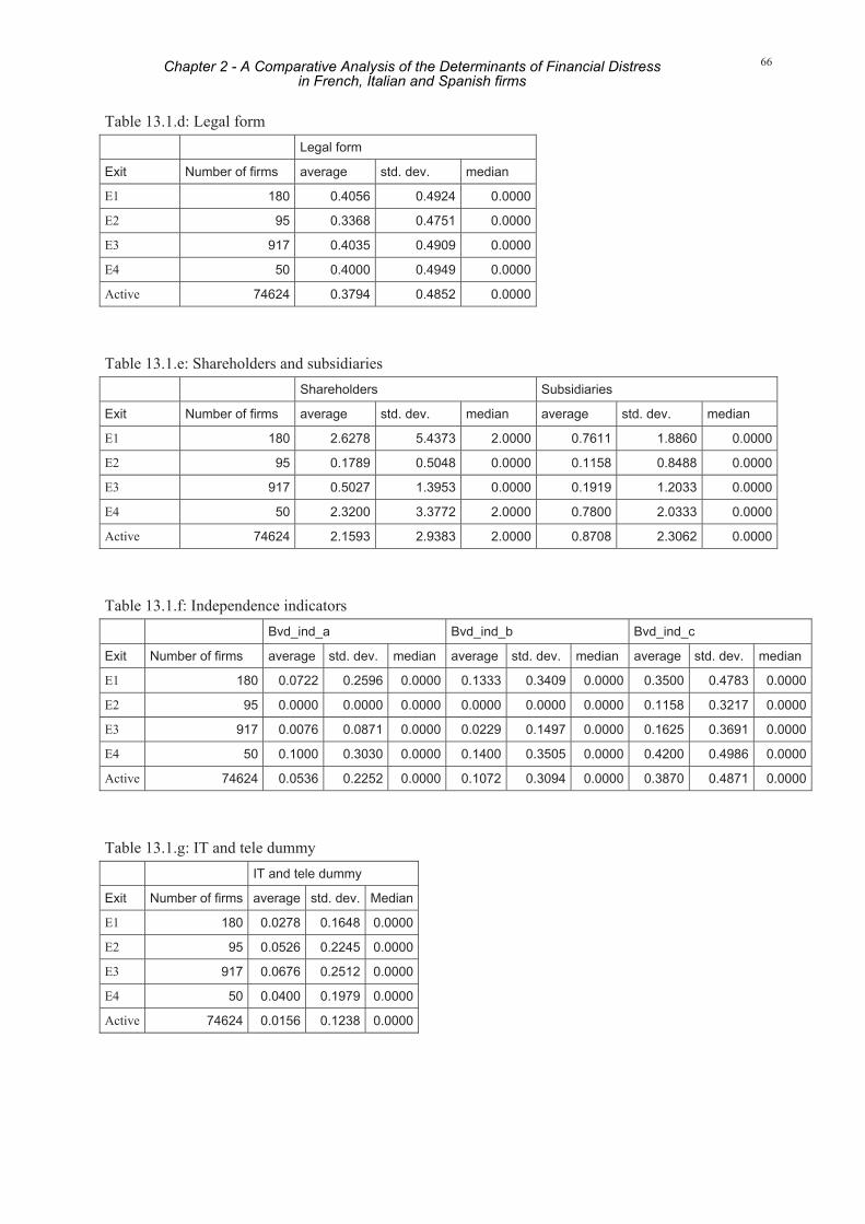
66

Table 13.1.d: Legal form Legal form

Exit Number of firms average std. dev. median

E1 180 0.4056 0.4924 0.0000

E2 95 0.3368 0.4751 0.0000

E3 917 0.4035 0.4909 0.0000

E4 50 0.4000 0.4949 0.0000

Active 74624 0.3794 0.4852 0.0000

Table 13.1.e: Shareholders and subsidiaries Shareholders Subsidiaries

Exit Number of firms average std. dev. median average std. dev. median

E1 180 2.6278 5.4373 2.0000 0.7611 1.8860 0.0000

E2 95 0.1789 0.5048 0.0000 0.1158 0.8488 0.0000

E3 917 0.5027 1.3953 0.0000 0.1919 1.2033 0.0000

E4 50 2.3200 3.3772 2.0000 0.7800 2.0333 0.0000

Active 74624 2.1593 2.9383 2.0000 0.8708 2.3062 0.0000

Table 13.1.f: Independence indicators Bvd_ind_a Bvd_ind_b Bvd_ind_c


E1 180 0.0722 0.2596 0.0000 0.1333 0.3409 0.0000 0.3500 0.4783 0.0000

E2 95 0.0000 0.0000 0.0000 0.0000 0.0000 0.0000 0.1158 0.3217 0.0000

E3 917 0.0076 0.0871 0.0000 0.0229 0.1497 0.0000 0.1625 0.3691 0.0000

E4 50 0.1000 0.3030 0.0000 0.1400 0.3505 0.0000 0.4200 0.4986 0.0000

Active 74624 0.0536 0.2252 0.0000 0.1072 0.3094 0.0000 0.3870 0.4871 0.0000

Table 13.1.g: IT and tele dummy IT and tele dummy

Exit Number of firms average std. dev. Median

E1 180 0.0278 0.1648 0.0000

E2 95 0.0526 0.2245 0.0000

E3 917 0.0676 0.2512 0.0000

E4 50 0.0400 0.1979 0.0000

Active 74624 0.0156 0.1238 0.0000


67

Table 13.1.h: Sector affiliation Mean

Exit Number of firms Dumman Dumorg Dumcon Dumfar Dummin

E1 180 0.0378 0.0167 0.1667 0.0111 0.0056

E2 95 0.2842 0.0211 0.0105 0.0000 0.0000

E3 917 0.2923 0.0632 0.0513 0.0218 0.0120

E4 50 0.2800 0.0200 0.1200 0.0000 0.0000

Active 74624 0.3559 0.0278 0.1191 0.0214 0.0120

Table 13.1.i: Sector affiliation Mean

Exit Number of firms Dumene Dumbus Dumpub Dumtraho Dumtra

E1 180 0.0000 0.0667 0.0278 0.2389 0.0889

E2 95 0.0105 0.1684 0.0000 0.3895 0.1158

E3 917 0.0120 0.1450 0.0153 0.2868 0.1003

E4 50 0.0000 0.0800 0.0000 0.4000 0.1000

Active 74624 0.0051 0.0945 0.0135 0.2902 0.0606


68

France

Table 13.2.a: France: Number of E1, E2, E3, E4 and active firms 2000 2001 2002 Total

E1 167 396 1140 1703

E2 48 686 675 1409

E3 2 22 39 63

E4 152 418 525 1095

Active 28757 34710 40796 104263

Total 29116 36232 43175 108533



E1 1703 22.2519 19.8680 16.0000 8.2535 0.6854 8.1236 E2 1409 22.0135 18.0559 17.0000 8.5188 0.7725 8.3705 E3 63 17.3968 14.1928 14.0000 8.0145 0.8903 8.0236 E4 1095 19.3434 17.1048 14.0000 8.3572 0.7533 8.2488 Active 104263 22.4788 17.9819 18.0000 8.4849 0.7303 8.3226

Table 13.2.c. (part 1): Earnings ratio and solvency ratio Earnings ratio Solvency ratio Exit Number of firms average std. dev. median average std. dev. median E1 1703 -0.0230 0.2305 0.0292 0.0585 0.3672 0.1121 E2 1409 0.0830 0.1580 0.0793 0.2586 0.3279 0.2584 E3 63 -0.0981 0.4989 -0.0494 -0.1278 0.8616 0.0757 E4 1095 -0.0184 0.2783 0.0333 0.1203 0.4181 0.1424 Active 104263 0.1020 0.1438 0.0962 0.3077 0.2574 0.2937

Table 13.2.c. (part 2): Loans to total assets ratio Loans to total assets Exit Number of firms average std. dev. median E1 1703 0.1117 0.1585 0.0543 E2 1409 0.0743 0.1335 0.0220 E3 63 0.1205 0.2305 0.0031 E4 1095 0.1088 0.1699 0.0389 Active 104263 0.0731 0.1153 0.0307


69



E1 1703 0.1632 0.3697 0.0000

E2 1409 0.1448 0.3520 0.0000

E3 63 0.1587 0.3684 0.0000

E4 1095 0.1489 0.3561 0.0000

Active 104263 0.1372 0.3441 0.0000



E1 1703 1.3030 1.4183 1.0000 0.3958 1.0441 0.0000

E2 1409 0.3385 0.7768 0.0000 0.0298 0.2365 0.0000

E3 63 0.8254 1.4204 0.0000 0.0794 0.3263 0.0000

E4 1095 0.5982 1.0652 0.0000 0.0758 0.4612 0.0000

Active 104263 1.3600 1.2720 1.0000 0.4583 1.2622 0.0000

Table 13.2.f: Independence indicator Bvd_ind_a Bvd_ind_b Bvd_ind_c


E1 1703 0.0411 0.1986 0.0000 0.0364 0.1874 0.0000 0.6312 0.4826 1.0000

E2 1409 0.0185 0.1346 0.0000 0.0106 0.1027 0.0000 0.1505 0.3576 0.0000

E3 63 0.0476 0.2147 0.0000 0.0476 0.2147 0.0000 0.2381 0.4293 0.0000

E4 1095 0.0228 0.1494 0.0000 0.0256 0.1579 0.0000 0.2785 0.4485 0.0000

Active 104263 0.0297 0.1697 0.0000 0.0318 0.1754 0.0000 0.6820 0.4657 1.0000



E1 1703 0.0464 0.2104 0.0000

E2 1409 0.0405 0.1971 0.0000

E3 63 0.0794 0.2725 0.0000

E4 1095 0.0922 0.2895 0.0000

Active 104263 0.0307 0.1726 0.0000


70



E1 1703 0.5079 0.0088 0.1133 0.0082 0.0029

E2 1409 0.2576 0.0234 0.0625 0.0099 0.0071

E3 63 0.3333 0.0000 0.0317 0.0159 0.0159

E4 1095 0.3306 0.0192 0.0648 0.0064 0.0055

Active 104263 0.3083 0.0222 0.0843 0.0123 0.0081



E1 1703 0.0000 0.0992 0.0123 0.1908 0.0564

E2 1409 0.0014 0.2229 0.0213 0.3329 0.0610

E3 63 0.0000 0.1905 0.0000 0.3492 0.0635

E4 1095 0.0018 0.2210 0.0110 0.2858 0.0539

Active 104263 0.0026 0.1320 0.0226 0.3494 0.0582


71

Italy

Table 13.3.a: Italy: Number of E1, E2, E3, E4 and active firms 2000 2001 2002 Total

E1 73 72 10 155

E2 6 2 16 24

E3 117 74 248 439

E4 9 10 46 65

Active 28083 32989 35977 97049

Total 28288 33147 36297 97732



E1 155 15.32258 10.26084 14 8.516675 0.751624 8.5368 E2 24 17.875 11.2687 18 8.835247 1.613305 8.885364 E3 439 20.96128 12.89192 18 8.945507 0.827272 8.930891 E4 65 11.33846 8.522538 9 8.756897 1.321122 8.823501 Active 97049 21.08392 13.72118 19 8.629584 0.812911 8.514991

Table 13.3.c (part 1): Earnings ratio and solvency ratio Earnings ratio Solvency ratio Exit Number of firms average std. dev. median average std. dev. median E1 155 -0.1685 0.3272 -0.0593 -0.1892 0.4706 -0.0127 E2 24 0.0712 0.0771 0.0762 0.2070 0.2359 0.1447 E3 439 0.0605 0.1868 0.0742 0.1817 0.3590 0.1744 E4 65 0.0703 0.0795 0.0671 0.2135 0.2465 0.1304 Active 97049 0.0979 0.1090 0.0882 0.2286 0.2084 0.1848

Table 13.3.c. (part 2): Loans to total assets Loans to total assets Exit Number of firms average std. dev. median E1 155 0.2065 0.2763 0.0967 E2 24 0.1881 0.1950 0.1707 E3 439 0.1581 0.2372 0.0738 E4 65 0.1124 0.1589 0.0022 Active 97049 0.1246 0.1578 0.0476


72


Exit Number of firms Average std. dev. median

E1 155 0.7290 0.4459 1.0000

E2 24 0.7083 0.4643 1.0000

E3 439 0.5330 0.4995 1.0000

E4 65 0.7231 0.4510 1.0000

Active 97049 0.6714 0.4697 1.0000


Exit Number of firms average std. dev. median Average std. dev. median

E1 155 0.5677 1.3437 0.0000 0.3290 1.2280 0.0000

E2 24 1.5417 1.8877 2.0000 0.2917 0.6903 0.0000

E3 439 0.7722 3.0689 0.0000 0.7631 1.8563 0.0000

E4 65 0.9385 2.0907 0.0000 0.2154 0.5726 0.0000

Active 97049 0.5776 1.5542 0.0000 0.4443 1.1794 0.0000

Table 13.3.f: Independence indicator Bvd_ind_a Bvd_ind_b Bvd_ind_c


E1 155 0.0129 0.1132 0.0000 0.0194 0.1382 0.0000 0.1613 0.3690 0.0000

E2 24 0.0417 0.2041 0.0000 0.0417 0.2041 0.0000 0.4583 0.5090 0.0000

E3 439 0.0205 0.1419 0.0000 0.0501 0.2184 0.0000 0.1572 0.3644 0.0000

E4 65 0.0154 0.1240 0.0000 0.0615 0.2422 0.0000 0.2000 0.4031 0.0000

Active 97049 0.0148 0.1206 0.0000 0.0407 0.1975 0.0000 0.1299 0.3362 0.0000


Exit Number of firms

Average std. dev. Median

E1 155

0.0645 0.2465 0.0000

E2 24

0.0833 0.2823 0.0000

E3 439

0.0364 0.1876 0.0000

E4 65

0.0154 0.1240 0.0000

Active 97049

0.0226 0.1486 0.0000


73



E1 155 0.5677 0.0065 0.1355 0.0065 0.0000

E2 24 0.6667 0.0000 0.0000 0.0000 0.0000

E3 439 0.5034 0.0137 0.0569 0.0023 0.0068

E4 65 0.4769 0.0000 0.0769 0.0308 0.0000

Active 97049 0.5236 0.0136 0.0747 0.0046 0.0074



E1 155 0.0000 0.0710 0.0065 0.1677 0.0387

E2 24 0.0000 0.0000 0.0000 0.2917 0.0417

E3 439 0.0046 0.0478 0.0137 0.3007 0.0478

E4 65 0.0154 0.0462 0.0000 0.3385 0.0154

Active 97049 0.0030 0.0511 0.0126 0.2663 0.0396


74

14. Appendix: The Construction of Sector Affiliation Codes

Table 14.a: Sector affiliation codes Sector Affiliation NACE-codes

1. Farming 01

2. Forestry 02

3. Fishing 05

4. Mining 10-14

5. Manufacturing 15-37

6. Energy (“Production of electricity, manufacturing of gas, collection, purification and distribution of water")

40-41

7. Construction (“Construction of buildings and civil engineering works, various contractors and other building completion”)

45

8. Trade and hotel (“Wholesale, retail, repair and hotels”) 50-52, 55

9. Transport 60-64

10. Business service (“Development and selling of real estate, renting, legal activities, advertising, etc."), (except 74.15: non-financial holding companies)

70-74

11. Public service activities (“General (overall) public service activities, education, hospital activities”)

75, 80, 85

12. Organisations, etc. (“Collection and treatment of waste, activities of business and employers organisations, etc., motion picture, video, radio, television, etc., laundering for industrial or commercial clients”)

90-93

Table 14.b: The construction of the IT and tele-dummy NACE codes included in the IT and tele-dummy Description of sector

3000 – 3100 Manufacture of office machinery and computers

3200 Manufacture of radio, television and communication equipment and apparatus

3220 – 3230 Manufacture of television and radio transmitters and apparatus for line telephony and line telegraphy

Manufacture of television and radio receivers, sound or video recording or reproducing apparatus and associated goods

6420 – 6421 Telecommunications

7200 – 7300 Computer and related activities

Hardware consultancy

Software consultancy and supply

Data processing


75

15. Appendix: Results

Tables 15.a, 15.b and 15.c show the parameter estimates for France, Italy and Spain. Tables 15.d, 15.e and 15.f present a detailed breakdown of the discriminatory power in the countries.

The fact that the parameters must be interpreted as contrasts between pairs means, for example, that the odds that an Italian private limited liability company will enter financial distress rather than staying active are about exp(0.4190)=1.52 the odds for Italian public limited liability companies. For the solvency ratio which in the French case has exp(-2.3606)=0.09, each 1-level increase in the variable multiplies the odds of moving into financial distress versus staying active by about 0.09.

The global tests (wald tests, not reported) for the effect of each variable on the outcome variable, controlling for the other variables in the models, shows that in the 1) French case none of the core variables and none of the proxies have no effect on the outcome variable, that in 2) Italian case one of the core variables (loans to total assets ratio) and three of the proxies (number of recorded shareholders, bvd_indep_a and bvd_indep_b) have no effect on the outcome variable, and that in the 3) Spanish case none of the core variables and two of the proxies (legal form and bvd_indep_b) have no effect on the outcome variable.

Table 15.a: Results for France E1 E2 E3 E4

Age 0.00302* 0.00212 -0.00745 -0.00308

Size -0.3265* 0.5722* -0.4964* 0.1710*

Earnings ratio -1.6054* -0.4369* -1.15674* -1.8075*

Solvency ratio -1.5832* -0.8419* -1.9564* -1.1897*

Loans to total assets 0.3169* -0.5846* -0.0394 0.4944*

Legal form 0.0624 -0.2267* -0.3305 -0.2054*

Shareholders -0.0214 -0.3424* 0.0862 -0.2355*

Subsidiaries 0.0355 -1.8568* -0.8478* -0.9966*

Bvd_indep_a 0.1973 -1.1061* -0.6731 -0.9097*

Bvd_indep_b -0.0924 -1.3081* -0.7056 -0.4851*

Bvd_indep_c -0.3653* -2.3551* -2.2554* -1.6785*

Note: A significance level of 5 pct. is chosen. Year dummies and sector affiliation dummies were included. Because the data was too sparse otherwise in some countries, a grouping of the sector affiliation dummies took place. The sector affiliation dummies that were included in the estimations were: Dumorgpub = dumorg + dumpub, dumcon, dumfarminene = dumfar + dummin + dumene, dumbus, dumtrahot, dumtra. France: In the first estimations age dummies were included. None of these turned out to be significant. In the final estimations no age dummies are included, only the variable age. Italy and Spain: In the first estimations a flexible baseline-hazard function was specified. This led to a quasi-complete separation of data points, meaning that a maximum likelihood estimate may not be possible to obtain, as the data is too sparse. The consequence of this was to use age in the estimations.


76

Table 15.b: Results for Italy E1 E2 E3 E4

Age -0.0298* -0.0164 -0.00493 -0.1149*

Size 0.2978* 0.2117 0.3954* 0.3110

Earnings ratio -2.4314* -1.2575 -1.3091* -1.3095

Solvency ratio -2.3606* 0.6237 -0.6816* 0.7455

Loans to total assets -0.2008 1.9005 0.1065 -0.4038

Legal form 0.4787* 0.5745 -0.3297* 0.0748

Shareholders 0.0258 0.0437 0.0269 0.0562

Subsidiaries -0.0954 -0.2823 0.0804* -0.2721

Bvd_indep_a -0.0391 1.5015 -0.0503 -0.1619

Bvd_indep_b -0.2694 0.2656 -0.0201 0.2981

Bvd_indep_c 0.0127 1.6508* -0.0817 0.2368


Table 15.c: Results for Spain E1 E2 E3 E4

Age 0.00784 0.0218* 0.00627* 0.00967

Size 0.0294 0.7983* 0.7497* -0.3548

Earnings ratio -1.1842* 0.0513 -1.4342* -2.0180*

Solvency ratio -0.9511* -1.5867* -0.4001* -0.2487

Loans to total assets 1.4822* 0.6268 0.0570 -0.5464

Legal form 0.1166 -0.3835 -0.0971 0.0524

Shareholders 0.0271 -1.9472* -0.7760* -0.0147

Subsidiaries -0.0516 -0.8504* -0.5788* 0.00860

Bvd_indep_a 0.1721 -11.7988 -1.5824* 1.1439*

Bvd_indep_b 0.0223 -9.9551 -0.4396 0.6974

Bvd_indep_c -0.3174 -0.1640 -1.0065* 0.4729



77

Table 15.d: Competing-risks model, detailed breakdown: France Model prediction:


Model prediction:



75 pct. (1,280 out of 1,703)


25 pct. (423 out of 1,703)

E2 (merger) Type 2 error: Wrong signal:

39 pct. (550 out of 1,409)


61 pct. (859 out of 1,409)


70 pct. (44 out of 63)


30 pct. (19 out of 63)

E4 (inactive (no precision)) Type 2 error: Wrong signal:

51 pct. (560 out of 1,095)


49 pct. (535 out of 1,095)

Active firms Type 2 error: Wrong signal:

28 pct. (29,347 out of 104,263)


73 pct. (76,070 out of 104,263)

Table 15.e: Competing-risks model, detailed breakdown: Spain Model prediction:


Model prediction:



76 pct. (137 out of 180)


24 pct. (43 out of 180)


45 pct. (43 out of 95)


55 pct. (52 out of 95)


36 pct. (330 out of 917)


64 pct. (587 out of 917)


48 pct. (24 out of 50)


52 pct. (26 out of 50)


32 pct. (23,717 out of 74,624)


67 pct. (50,907 out of 74,624)


78

Table 15.f: Competing-risks model, detailed breakdown: Italy Model prediction:


Model prediction:



88 pct. (137 out of 155)


12 pct. (18 out of 155)


25 pct. (6 out of 24)


75 pct. (18 out of 24)


26 pct. (116 out of 439)


74 pct. (323 out of 439)


25 pct. (16 out of 65)


75 pct. (49 out of 65)


29 pct. (28,145 out of 97,049)


71 pct. (68,904 out of 97,049)


"All models are wrong.

Some models are useful."

George E. P. Box

CHAPTER 3

Anne Dyrberg Rommer*

Testing the Assumptions of Credit-scoring Models

* This chapter is based on A. Dyrberg Rommer, 2005, Testing the Assumptions of Credit-scoring Models, Working Paper no. 28, Danmarks Nationalbank. The author would like to thank Hans Christian Kongsted, Jesper Berg, Karsten Biltoft, Steen Winther Blindum, Anders Møller Christensen, Bo Honoré, David Lando, Jesper Rangvid and colleagues at the Danish Central Bank for commenting on this or earlier versions of the paper and seminar participants at the Danish Graduate Program in Economics workshop held 13. - 14. November 2003, Centre for Applied Microeconometrics (University of Copenhagen) seminar held 18. November 2003, Danish Central Bank seminar held 27. November 2003. Corresponding address is Anne Dyrberg Rommer, Financial Markets, Danmarks Nationalbank, Havnegade 5, DK-1093 Copenhagen, Denmark. Phone: + 45 33 63 63 63. Email: [email protected]

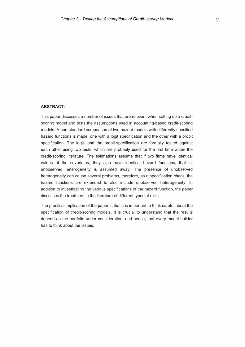
2

ABSTRACT:

This paper discusses a number of issues that are relevant when setting up a credit-scoring model and tests the assumptions used in accounting-based credit-scoring models. A non-standard comparison of two hazard models with differently specified hazard functions is made: one with a logit specification and the other with a probit specification. The logit- and the probit-specification are formally tested against each other using two tests, which are probably used for the first time within the credit-scoring literature. The estimations assume that if two firms have identical values of the covariates, they also have identical hazard functions, that is, unobserved heterogeneity is assumed away. The presence of unobserved heterogeneity can cause several problems, therefore, as a specification check, the hazard functions are extended to also include unobserved heterogeneity. In addition to investigating the various specifications of the hazard function, the paper discusses the treatment in the literature of different types of exits.

The practical implication of the paper is that it is important to think careful about the specification of credit-scoring models. It is crucial to understand that the results depend on the portfolio under consideration, and hence, that every model builder has to think about the issues.

Chapter 3 - Testing the Assumptions of Credit-scoring Models

3

1. Introduction .......................................................................................................4

2. Data and the Treatment of Exits .......................................................................7

3. The Estimation Problem..................................................................................12 3.1. Derivation of the Sample Likelihood...............................................12 3.2. Derivation of an easy Estimation Method.......................................15 3.3. Expression for the Hazard Rate .....................................................15 3.4. Unobserved Heterogeneity and its Consequences........................16 3.5. Expression for the Hazard Rate with Unobserved Heterogeneity..17 3.6. Specification Tests..........................................................................18

4. Results ............................................................................................................20 4.1. The Specification of the Hazard Function ......................................21 4.2. Testing for Unobserved Heterogeneity...........................................23 4.3. Parameter Estimates ......................................................................25

5. Prediction ........................................................................................................27

6. Conclusion ......................................................................................................31

7. LITERATURE..................................................................................................34


4

1. Introduction The purpose of this paper is to discuss a number of issues that are relevant when setting up a credit-scoring model and to test the assumptions used in accounting-based credit-scoring models. Specification issues are important to consider, as more powerful models are more profitable than weaker ones, c.f. Stein (2005). The topic is important not only for individual credit institutions, who use credit-scoring models to find out which clients they want to offer loans and to detect clients that are likely to default at an early stage, but also for banking supervisors, who are regulating banks, for central banks, who are analyzing the developments in the financial sector and accordingly assessing financial stability developments, and for other agents, e.g. management, financial analysts, investors and auditors, who also need timely warnings.

In addition to the strong interest in the topic of credit-scoring from the policy side (from central banks and banking supervisors) and from a more practical front (from e.g. credit institutions, managers, investors and auditors), there is also a strong academic interest in the topic. This is seen by the vast amount of literature on credit-scoring models. Some of the recent studies are Hillegeist, Keating, Cram and Lundstedt (2004), Jones and Hensher (2004), Dyrberg (2004) and Grunert, Norden and Weber (2005). Examples of surveys of the developments in the area include Zavgren (1982), Jones (1987), Dimitras, Zanakis and Zopounidis (1996), Altman and Saunders (1998) and Balcaen and Ooghe (2004). Some of the often-quoted parametric credit-rating studies are Altman (1968), Ohlson (1980) and Shumway (2001). Examples of non-parametric credit-rating studies are Frydman, Altman and Kao (1985), Tam and Kiang (1992) and Dimitras, Slowinski, Susmaga and Zopounidis (1999).

Altman (1968), Ohlson (1980) and Shumway (2001), which are some of the often-quoted parametric credit-rating studies, c.f. above, suggest the use of multivariate discriminant analysis, the logit model and the hazard model, respectively. These methods are the standard methods within the parametric credit-scoring literature. Accordingly, they are used in a number of papers. For example, discriminant analysis is used in Bardos (2001), Cifarelli and Corielli (1988), Betts and Belhoul (1987), Dambolena and Khoury (1980) and in Altman, Haldeman and Narayanan (1977), and logit models are used in Moody’s Investors Service (2001a), Moody’s Investors Service (2001b), Moody’s Investors Service (2002), Jiménez and Saurina (2004) and Corcóstegui, González-Mosquera, Marcelo and Trucharte (2003). Hazard models are used in Hillegeist, Keating, Cram and Lundstedt (2004), Campbell, Hilscher and Szilagyi (2005) and Chava and Jarrow (2004). In addition to the standard methods (discriminant analysis, logit models and hazard models), other parametric methods have been used occasionally, e.g. the probit model. Papers, which consider probit models, are e.g. Bunn and Redwood (2003), Skogsvik (1990) and Zmijewski (1985).


5

A number of studies compare various estimation strategies, c.f. Altman, Marco and Varetto (1994), Back, Laitinen, Sere and Wezel (1996), Begley, Ming and Watts (1996), Lo (1986), Frydman, Altman and Kao (1985) and Lennox (1999). This paper is a methodological paper along the lines of these papers. Most of the papers have compared logit analysis to other estimation methods such as discriminant analysis and various non-parametric techniques. Here a non-standard comparison of two hazard models with differently specified hazard functions is made: one with a logit specification and the other with a probit specification. The specification of the credit-scoring model as a hazard model allows us to include information leading up to “financial distress”. The logistic distribution is similar to the normal, except in the tails, and so the logit and the probit model tend to give similar probabilities, except in the tails. The tails of the logistic distribution are considerably heavier than the tails of the normal distribution, i.e. in the tails of the logistic distribution, the probabilities are larger compared to the normal distribution. The comparison of the two distributions is relevant, as the properties at the tails of the distributions are at focus here. The only other paper we have found, which compares the logit and the probit model (though not in the framework of a hazard model), is Lennox (1999).

We use the Davidson and MacKinnon (1993:492) test-procedure and the Silva (2001) test-procedure to test the two specifications for the hazard function. Lennox (1999) compares the results from the estimation of a logit and a probit model. He does not set up a hazard model and he does not provide any tests for the specification of the credit-scoring model as a logit or probit model. As we test the logit and the probit specification for the hazard function, our approach extends his study. To the best of our knowledge this is the first time, these tests have been used within the credit-scoring literature.

The estimations assume that if two firms have identical values of the covariates, they also have identical hazard functions, that is, unobserved heterogeneity is assumed away. The presence of unobserved heterogeneity can cause several problems, therefore, as a specification check, the hazard functions are extended to also include unobserved heterogeneity. Unobserved heterogeneity is not modelled in Lennox (1999). The only other studies we know of, which models unobserved heterogeneity in a credit-scoring setting, are Kaiser (2001), Bernhardsen (2001) and Jones and Hensher (2004).

In addition to the investigations of the various specifications of the hazard function (logit and probit specification with and without unobserved heterogeneity) the treatment of different types of exits in the literature is discussed. There are recent examples of studies within the credit-scoring and the industrial organization literature, which still do not distinguish between exit types (e.g. Bunn and Redwood (2003), Pérez, Llopis and Llopis (2004), Mata and Portugal (2002) and Kimura and Fujii (2003)). Therefore, it will be shown what the consequences are of setting up


6

1) a hazard model where the event financial distress is modelled and where firms that exit for other reasons than financial distress are treated as censored or no longer observed and 2) a hazard model where the general exit event is modelled (i.e. not split up on exit type). To the best of our knowledge no other paper provides the estimations of a hazard model, where firms in financial distress are modelled and where the other forms of exits are treated as censored versus a model, which pool the three modes of exit (financial distress, voluntary liquidation and mergers and acquisitions etc.). Dyrberg (2004), Harhoff, Stahl and Woyde (1998) and Schary (1991) are the papers, which are closest to our paper in this respect, c.f. section 2.

The data set used in the estimations is unique compared to most other credit-scoring studies and industrial organisation studies. It includes the whole population of Danish public and private limited liability companies, which existed between 1995 and 2001. Most are small and medium-sized enterprises. The panel data set covers all non-financial sectors of the Danish economy. Included in the estimations are around 30,000 firms and more than 150,000 firm-year observations. There are 2,617 firms in financial distress, 907 voluntarily liquidated firms, and 1,233 firms that are acquired/have merged with other firms, etc. In comparison, Lennox (1999) is not able to follow each firm throughout his observation window. His sample is also smaller than ours. Compared to our more than 30,000 firms and 2,617 defaults, he uses a sample, which includes 949 firms and 90 defaults.

The overall conclusions from the analysis are that there does not seem to be any major difference between the hazard model with the logit and the probit specification, that unobserved heterogeneity seems to be unimportant, but that the results differ depending on the event, which is modelled (financial distress versus pooled exits). The observations leading to these conclusions are discussed more extensively in section 6.

The practical implication of the paper is that it is important to think careful about the specification of credit-scoring models. Here the specification issues are highlighted and investigated using an extensive data set on Danish non-financial sector firms. It is crucial to understand that the results depend on the portfolio under consideration, and hence, that every model builder has to think careful about the issues. This paper provides a framework for such investigations.

The paper is divided into 6 sections. Section 2 presents the data, which is used in the estimations, and it discusses the way different exits are modelled in the literature. In section 3 the estimation problem is set up and tests for the specification of the hazard function are presented. Section 4 reports the results, including the outcome of the tests for the specification of the hazard function and the parameter estimates, which are obtained, when 1) the financial distress event and 2) the exit event is modelled. Section 5 discusses prediction in credit-scoring


7

models, and it evaluates the predictive ability of the models. Finally, section 6 concludes.

2. Data and the Treatment of Exits The data set used in the estimations covers all Danish public limited liability companies and private limited liability companies that existed in the period from 1995 to 2001. As it covers the whole population of public and private limited liability companies, it differs from the data set available to individual credit institutions, which wants to set up credit-scoring models. Some of the issues, which are necessary for individual credit institutions to think about, but which are not a problem in the set up here in this paper, are sketched in box 2.a (drop-outs) and box 2.b (reject inference).

The main part of the data set used in the estimations is received from the Danish credit-rating agency KOB A/S. It comprises information on financial issues as well as non-financial issues. On top of the information received from KOB A/S, the data base is augmented to also include whether or not the company is 1) an ultimate parent company, 2) a wholly owned subsidiary, 3) quoted on the stock exchange, 4) owned by the public, 5) owned by a fund and 6) a concentration index (measuring the concentration of the various sectors).

Box 2.a: Drop-outs in credit institutions portfolios

Although not discussed in the literature, individual banks have customers that may drop-out

of the sample, while they are still active. There can be different reasons for the drop-out.

One hypothesis could be that some firms choose another bank, because it offers better

service or a better price (perhaps because they are bundling their activities). These

companies may be well-performing companies, which show no indication of financial

distress. Another hypothesis could be that some companies change to another bank,

because they are asked to by their current bank, i.e. that their current bank could suspect

that they would soon enter financial distress. If it is not known by banks, why firms drop out

of their portfolio, it is crucial for banks to find out what type of drop-outs they observe, and

accordingly, what assumptions they can make about the drop-outs in order to obtain

consistent estimates, when they set up their credit-scoring models.

Rommer (2005b:17ff) provides a framework for analyzing drop-outs and interested

readers are referred to the paper for details on how she analyses drop-outs versus firms that

do not drop out by 1) testing for equal means of a number of characteristics, 2) by

estimation of drop-out probits and 3) by estimation of credit-scoring models with and

without the drop-outs.


8

Box 2.b: Reject inference

In the raw data set there are 603,956 firm-year observations. After the exclusion of holding companies and financial firms and after making some corrections to the database, there are 430,422 firm-year observations left. The panel used in the estimations consists of companies that were incorporated in the period 1995 – 2001 with at least 5 employees the year they are included in the sample and with a balance sheet of at least kr. 500,000 (flow sampled companies), and companies that were active in 1995 but were incorporated before 1995 with at a balance sheet of at least kr. 500.000 and 5 employees in 1995 (the stock sampled companies). The panel consists of 168,778 firm-year observations, covering 32,453 firms. Due to missing variables, the final number of firm-year observations in the estimations is 168,350, covering 32,365 firms.

Credit-scoring models are used in credit institutions to evaluate loan applicants in order to

assess whether or not a loan should be granted. The output of a credit-scoring model is an

estimate of the probability that a specific loan applicant will default within a certain

horizon, usually a one-year horizon.

Credit scoring-models have received new interest, as their output, the PD (probability of

default) can now serve as an input in the calculation of a credit institutions minimal capital

requirement, if the credit institutions choose to calculate their minimal capital requirement

using one of two different internal ratings-based approaches (IRB), c.f. BCBS (2004) and

Borup, Kurek and Rommer (2005). In the Basel II proposal, BCBS (2004:91), it is specifically

stated that “Internal ratings and default and loss estimates must play an essential role in the

credit approval, risk management, internal capital allocations, and corporate governance

functions of banks using the IRB approach. Ratings systems and estimates designed and

implemented exclusively for the purpose of qualifying for the IRB approach and used only to

provide IRB inputs are not acceptable. It is recognized that banks will not necessarily be

using exactly the same estimates for both IRB and all internal purposes. For example, pricing

models are likely to use PDs and LGDs [loss given default] relevant for the life of the asset.

Where there are such differences, a bank must document them and demonstrate their

reasonableness to the supervisor.”

The idea behind Basel II is that the credit institutions should not only develop credit-

scoring models and use these to calculate their minimal capital requirements, but that these

models should also play an essential role in the credit approval process. One issue, which is

not highlighted in the Basel II proposal, is that it may not be ideal to use the same credit-

scoring model to calculate the probability of default and to approve new loans. The reason

for this is the typical sample selection argument. If only obligors that already have been

approved for a loan are taken into account in the estimations, then it is not appropriate to

use the same model to consider new applications. If the models estimated using data on

already approved applicants are applied to all applicants, then a sample selection bias is

introduced.

Feelders (2003), among others, has a theoretical discussion of the sample selection issue,

also called the reject inference problem (without making reference to Basel II). The

literature is divided into two camps. Some of the estimations show that it does not make a

big difference to adjust for the reject inference problem. An example is Crook and Banasik

(2004) (consumer credit-scoring problem). Others find that it does make a difference to

adjust for the reject inference problem. These include Chen and Åstebro (2003) and

Roszbach (2003) (firm credit-scoring problems) and Chen and Åstebro (2001) and Greene

(1998) (consumer credit-scoring problems).


9

Note the difference between flow and stock sampled companies. The stock sampled companies are the ones that are active, when they are included in the sample. The flow sampled companies are the ones that are incorporated at some point in the observation window, which spans from 1995-2001. Hence, the difference between flow and stock sampled companies is that the whole history of the stock sampled companies is not observed, whereas the whole history of the flow sampled companies is observed. Both the flow and the stock sampled firms can be right censored. Only stock sampled firms are left truncated (i.e. not observed from the beginning of the spell, but with a known incorporation data). For further details see e.g. D'Addio and Rosholm (2002) and Dyrberg (2004).

Table 2.a: Number of firms

Financial distress (E1)

Voluntary liquidations (E2)

Mergers and acquisitions etc. (E3)

Active Total

1995 0 0 0 18853 18853

1996 372 87 177 20684 21320

1997 348 110 156 22008 22622

1998 347 129 195 23422 24093

1999 453 124 211 25000 25788

2000 618 148 226 26415 27407

2001 479 309 268 27639 28695

Total 2617 907 1233 164021 168778

Source: Dyrberg (2004)

An overview of the data set is seen from table 2.a, which shows the number of active firms every year and the number of firms that exit because of financial distress (E1), voluntary liquidation (E2), and mergers and acquisitions etc. (E3). Most firms exit because they are financially distressed. Voluntary liquidations account for the smallest number of exits. Rommer (2005a) and Phillips and Kirchhoff (1989) discuss the distinction between voluntary and involuntary exits.

Table 2.b summarizes the predictors used in the estimations. These are the same predictors that were used in Dyrberg (2004). They are divided into core variables, proxy variables, and controls. Core variables are variables that are usually used in credit-scoring studies. The proxy variables serve as proxies for inherently unobserved variables. Controls are included to take into account the macroeconomic effects and sector affiliation etc. As the focus in this paper is on


10

the methodology behind credit-scoring models and not on the selection of predictors and further details about the data set, for more on that, the reader is referred to Dyrberg (2004), which has extensive discussions of both issues.

Table 2.b: Predictors

Variables Firm Age (dummies) (reference category: firms that are one year old) Short-term debt to total assets Return on net assets Solvency ratio

CORE

VARIABLES

Firm size Firms that are not diversified (reference category) Diversification 2 sectors (related business) Diversification 3–9 sectors (related business) Diversification 2 sectors (unrelated business) Diversification 3–9 sectors (unrelated business) Local authority group 1 (reference category) Local authority group 2 Local authority group 3 Local authority group 4 Local authority group 5 Concentration Firms that are not owned by the public (reference category) Owned by the public (dummy) Firms that are not owned by the a fund (reference category) Owned by a fund (dummy) Firms that are not ultimate parent companies (reference category) Ultimate parent companies (dummy) Firms that are not wholly owned subsidiaries (reference category) Wholly owned subsidiaries (dummy) Public limited liability company (reference category) Private limited liability company (dummy) Firms that are not publicly traded (reference category) Publicly traded companies (dummy)

PROXIES

Firms without critical comments from the auditors (reference category) Critical comments from the auditors (dummy)

Year dummies: Year 1996 (reference category), Year 1997, Year 1998, Year 1999, Year 2000, Year 2001 Sector affiliation dummies: Farming, Forestry, Fishing, Mining, Manufacturing (reference category), Energy, Construction, Trade and hotel, Transport, Business service, Public service activities, Organisations, Not stated, Unknown. IT dummy (those firms that are considered as IT or tele-companies have, on top of the sector dummies, an IT dummy equal to 1, all other firms have an IT dummy equal to 0)

CONTROLS

Primary bank dummies: Some firms register a Primary Bank connection in one of the following four categories (see Dyrberg (2004:section 7) for further details): Category 1, Category 2, Category 3, Category 4, Some firms do not register a primary bank connection (reference category)


11

In the credit-scoring literature, active firms and financially distressed firms only are most often modelled (see e.g. Beaver (1966), Altman (1968) and Ohlson (1980)). Exceptions are Schary (1991) and Dyrberg (2004), who both advocate for a richer discussion of the determinants of exits. They distinguish between bankruptcy, voluntary liquidation, and mergers and acquisitions and estimate the credit-scoring models as a competing-risks model. Shumway (2001) sets up a hazard model and treats firms that exit for other reasons than financial distress as censored or no longer observed, when they leave the sample, i.e. he groups active firms and firms that are voluntarily liquidated, and firms that have merged or have been acquired by other firms etc. Bunn and Redwood (2003) consider a firm as failed in a particular year if its company status is ”in receivership, liquidation or dissolved, and its last reported accounts were in the previous year. This definition includes voluntary liquidation and dissolution where there may be no risk of default, but we are unable to distinguish between voluntary and compulsory failures in our data. … We do not consider being taken over to be a failure”, i.e. out of necessity Bunn and Redwood (2003) group firms in financial distress and voluntarily liquidated firms.

In the industrial organization literature there has been some attempts to study the factors, which lead firms to exit, split up on type of exit, c.f. Harhoff, Stahl and Woyde (1998), Köke (2001), Prantl (2003) and Bhattacharjee, Higson, Holly and Kattuman (2004). These four mentioned studies distinguish between two of the three mentioned exit types. Despite the fact that these papers show that it is important to distinguish between exit types, a number of recent industrial organization studies still consider exits in general, i.e. not split up on exit type. Some of these recent studies are Pérez, Llopis and Llopis (2004), Mata and Portugal (2002) and Kimura and Fujii (2003). Other studies are Audretsch and Mahmood (1994), Audretsch and Mahmood (1995) and Mata et al. (1995).

As there are recent examples of studies within the credit-scoring and the industrial organization literature, which still do not distinguish between exit types, it will be shown what the consequences are of setting up 1) a hazard model where the event financial distress is modelled and where firms that exit for other reasons are treated as censored or no longer observed and 2) a hazard model where the general exit event, i.e. not split up on exit type, is modelled. To the best of our knowledge no other paper provides such estimations. Dyrberg (2004), Harhoff et al. (1998) and Schary (1991) are the papers, which are closest to our paper. Harhoff et al. (1998) and Schary (1991), who distinguishes between two modes of exit (bankruptcies and voluntary liquidations) and three modes of exit (bankruptcies, voluntary liquidations, and mergers and acquisitions), respectively, estimate a competing-risks model and a model with pooled exits. None of the two studies provide estimates for a hazard model, which models financial distress and treats all other exits as censored or no longer observed, when they leave the sample. Dyrberg (2004), who distinguishes between three modes of exit


12

(bankruptcies, voluntary liquidations, and mergers and acquisitions, etc.), estimates a competing-risks model and a hazard model, where firms in financial distress are the event, and where all other exits are treated as censored or no longer observed, when they leave the data set. She does not provide estimates for a hazard model, which estimates the probability of the pooled exit event.

Another paper, which is along the lines of our paper, is Honjo (2000). He argues that by concentrating on firms in financial distress, he hopes to identify more significant factors, such as post-entry performance, compared to the studies, which model exits, i.e. treat all types of exits the same way.1 Honjo (2000) does not show what his results would have been, had he included firms that exit for other reasons than financial distress. By reporting the results (parameter estimates and predictive ability) from estimations where we model 1) firms in financial distress and 2) exits, we show what the consequences are of modelling either event.

3. The Estimation Problem Various statistical estimation methods have been suggested in the credit-scoring literature, c.f. the introduction. In this paper the focus is on the parametric estimation method, which is suggested in Shumway (2001), namely the hazard model. Shumway (2001) suggests the use of the hazard model, as it solves some of the econometric problems of the single-period logit approach that is suggested in Ohlson (1980). A particular important property of the hazard model is that it includes information on how long a firm survives with a set of characteristics.

We will investigate various specifications for the hazard function, namely the logit and the probit specification with and without unobserved heterogeneity.

In the following sections we set up the estimation problem, discuss the various specifications for the hazard functions and present the tests, which are used to test the different specifications against each other.

3.1. Derivation of the Sample Likelihood The sample likelihood for the hazard model is derived in this section, which builds on Jenkins (1995). We derive the sample likelihood for the case, when one has discrete data. In this respect, note, that the data, which is used in the estimations

1 Honjo (2000:560) is interested in investigating the post-entry performance of new firms, in particular,

the business failure of new firms over time: "Following the analytical framework used by Audretsch and Mahmood (1994), (1995) and Mata et al. (1995), we estimate determinants of business failure among new manufacturing firms in Tokyo during 1986-1994. However, whereas these previous studies dealt with exits, we analyze business failures, which may be regarded as special cases of exits, that is, exits without solvency. Firms exit for different reasons: some may exit voluntarily while they are still gaining profits, but others are forced to exit due to business failure. By concentrating on the latter ones, this paper, it is hoped, will be able to identify more significant factors, such as post-entry performance." Honjo (2000) defines firms without solvency as those firms, which have ceased operations with total debt more than 10 million yen. The data on failed firms include the firms that voluntarily compromised with creditors and ceased operations. Honjo (2000) does not consider firms that exit for other reasons than financial distress.


13

(and presented in section 2), is, what in the literature is called grouped duration data. Information on the firms is obtained once a year, when the financial statement is handed in. With grouped duration data one can assume that durations are intrinsically discrete and treat them accordingly, or alternatively, one may attempt to relate the model to an underlying process in continuous time. Here data is treated as if it was intrinsically discrete.

The probability that a firm ends up as an event (e.g. a financially distressed firm) at time 1T is

)()( 1 tTprobtTprob i === ,

where iT is a discrete random variable representing the time at which the end of the spell occurs, also called the event time. This is an unconditional probability, which can be rewritten as a product of conditional probabilities. Define the hazard rate, ith , as

);( itiiit XtTtTprobh ≥== ,

where itX is a vector of regressor variables which may vary with time. For both the stock and flow sampled firms, the probability of experiencing an event in year t, the unconditional probability, is

∏∏=

−

=

−−=−==t

i

t

ititiiti hhhhhtTprob1

1

1

)]1()1/([)1()(τ

ττ

τ

where τ denotes the incorporation date of the firm.

The probability of surviving beyond period t, the survivor function, is

∏=

−=>t

ii htTprob1

)1()(τ

τ

To motivate the derivation of the sample likelihood for the stock sampled (left truncated) firms consider a firm, i, which was incorporated in 1992, and which is still active in 1998. The unconditional probability of the firm still being active in 1998 is then

∏=

−−−=−=>t

iiiii hhhhtTprob1

1992,1997,1998, )1)...(1)(1()1()(τ

τ ,

whereas the probability of still being active, conditional on not having left the sample before 1995, when the firm is observed for the first time (called time b) is

)1)...(1()1)...(1)(1(

)1()1(1992,1994,

1992,1997,1998,

ii

iiisb

btitiii hh

hhhhbTstTprob

i

−−−−−

=−=−>+> ∏+

=


14

= )1)(1)(1)(1( 1995,1996,1997,1998, iiii hhhh −−−−

is indicates how many years each firms is observed.

The probability of experiencing the event in 1998, conditional on not having left the sample before 1995, is

∏+

=+

+

−−−−

=−−

=−>+=i

i

i

sb

bt ii

iiiit

sib

sibiii hh

hhhh

hh

bTstTprob)1)...(1(

)1)...(1)(()1(

1)1(

1992,1994,

1992,1997,1998,

= )1)(1)(1)(( 1995,1996,1997,1998, iiii hhhh −−−

It is seen that the conditioning of the survivor probabilities for the stock sampled firms is handled via a “cancelling” of terms. It is important to note, that a firm only contributes with as many observations as there is in the data set. The flow sampled firms are observed from the incorporation date (=when the firm is first observed at time b) and contributes from that time on, altogether is years. This is also seen from the equations.

The likelihood of observing the event history data for the whole sample can now be constructed. The likelihood is

∏ ∏∏=

−+

=

+

=+

+

⎥⎥

⎦

⎤

⎢⎢

⎣

⎡⎥⎦

⎤⎢⎣

⎡−

⎥⎥⎦

⎤

⎢⎢⎣

⎡−

−=

n

i

sb

btit

sb

btit

sib

sibi

ii

i

i

i hhh

hL

1

)1(

)1()1(1

δδ

1=iδ is defined as firms with completed spells and 0=iδ is defined as those with uncompleted spells. When the event financial distress is modelled, the firms with uncompleted spells are the ones, which are still active at the end of the observation window, or those which gets censored, e.g. because they leave the sample for other reasons than financial distress. When the exit event is modelled, the firms with uncompleted spells are the ones, which are active at the end of the observation window.

is indicates how many years each firms is observed and isb + refers to the point in time, when a firm leaves the database.

The log likelihood function is then

∑ ∑∑= =

+

=+

+ −+⎥⎥⎦

⎤

⎢⎢⎣

⎡

−=

n

i

n

i

sb

btit

sib

sibi

i

i

i hh

hL

1 1)1log(

1loglog δ

This specification of the likelihood function gives the probability that a particular firm experiences an event (either financial distress or exit, depending on which of the two we are modelling).


15

3.2. Derivation of an easy Estimation Method Using the above log likelihood function, Jenkins (1995:133) shows how to derive an easy estimation method. He defines a variable 1=ity if isbt += and 1=iδ , and 0=ity otherwise. Using the ity as indicator variable, the log-likelihood function can now be rewritten as

∑∑∑∑=

+

==

+

=

−+−=n

i

sb

btit

n

i

sb

btititit

ii

hhhyL11

)]1log[()]1/(log[log .

There are two important things to notice. One is (as mentioned above) that each firm contributes with as many observations as it has years at risk of exiting. The other is that the creation of multiple observations from each firm follows directly from factoring the likelihood function for the data. Each of the terms may be treated as though it came from a distinct, independent observation.

The log likelihood function has the same form as the standard log-likelihood function for regression analysis of a binary variable, in this case ity . Straightforward calculations give that the log likelihood function can be written as

∑∑∑∑=

+

==

+

=

−−+=n

i

sb

btitit

n

i

sb

btitit

ii

hyhyL11

)1log()1()log(log

3.3. Expression for the Hazard Rate Before the model can be estimated, the specification has to be completed by assuming an expression for the hazard rate. Below two different specifications will be presented. For now it is assumed that the specifications for the hazard functions capture all differences between firms using observed explanatory variables.

Let itX characterize the covariates, including the baseline hazard function. The baseline hazard function can be specified parametrically and non-parametrically. A non-parametric specification is preferred as any inconsistency caused by misspecification is then avoided. In the estimations, dummies for each age (up to a dummy with companies that are 30 years old or more) are included (the reference category is firms that are 1 year old). Note the difference between the age of the specific companies and the time dummies that control for the macroeconomic environment. Let β denote the coefficients of the covariates, which may be time-varying.

Having introduced itX and β , the specifications for the hazard function can now be presented. The suggested specifications are the logit and the probit. The logistic distribution is similar to the normal (except in the tails, which are considerably heavier, i.e. in the tails of the logistic distribution, the probabilities are larger compared to the normal distribution), and so the logit and the probit model tend to give similar probabilities, except in the tails, c.f. Greene (2003:667). Greene


16

(2003:667) also notes, that one would expect different predictions from the logit and the probit model, if the sample contains very few responses or non-responses. As we are in the tails of the distribution and as our sample contains very few responses compared to non-responses, it is worth investigating, whether the usual conclusion holds, namely that it is difficult to provide practical generalities on which model to choose (Greene (2003:667)).

The logit specification for the hazard function is:

ititititit XhhXh ')]1/(log[]]'exp[1/[1 ββ =−⇔−+=

The probit specification for the hazard function is:

itit Xh ')(1 β=Φ−

where )(1ith−Φ is the inverse cumulative distribution function of a standard normal

variable.

As the true hazard function is not known, there is no guarantee that any of the specifications represent the true specification of the hazard.

3.4. Unobserved Heterogeneity and its Consequences The hazard models presented above assumes that if two firms have identical values on the covariates, they also have identical hazard functions, that is, all differences between firms are assumed to be captured using observed explanatory variables, or, in other words, unobserved heterogeneity is assumed away. In Dyrberg (2004) it is argued that the assumption perhaps is more reasonable in estimations, which uses the data set presented and used in Dyrberg (2004) (as well as here) than in most cases, due to the fact several proxies are used for the variables that are inherently unobservable.

The probit and the logit specification for the hazard function are extended to also include unobserved heterogeneity. The estimation with unobserved heterogeneity can be seen as a specification check. The only other studies we know of, which models unobserved heterogeneity in a credit-scoring setting, are Kaiser (2001), Bernhardsen (2001) and Jones and Hensher (2004).

The presence of unobserved heterogeneity can cause several problems. The most serious problem is that the unobserved heterogeneity tends to produce estimated hazard functions that decline with age even when the true hazard is not declining for any individual in the sample (Kiefer (1988:671f)). Figure 3.4 sketches the effect of unobserved heterogeneity. The figure illustrates a case where all firms can be divided into two groups. One group consists of firms with a high and constant hazard (and with incompetent managers), and the other group consists of firms with a low and constant hazard (and with competent managers). When estimating the hazard function for the whole sample, the empirical hazard function starts out


17

midway between the two hazards and then declines until it approaches the lowest hazard as an asymptote. The estimated hazard captures a composition effect (the remaining sample is increasingly made up by firms with low hazards). The estimated hazard rate declines, even though the true hazards are constant.

A natural question is whether or not one can rely on the estimates of β in the presence of unobserved heterogeneity (see Allison (2001)). If the unobserved components are correlated with the measured covariates, then the coefficients may be severely biased. If the unobserved components are independent of the measured covariates (random effects) then the unobserved heterogeneity tends to attenuate the estimated coefficients towards 0. Both situations are undesireable. Nonetheless, the last case is “better” than the former, as we at least know, how the unobserved heterogeneity affects the parameter estimates.

Figure 3.4: Unobserved heterogeneity (composition effect)

3.5. Expression for the Hazard Rate with Unobserved Heterogeneity The specifications of the hazard functions are extended to incorporate unobserved heterogeneity (denoted iu ). The probit specification for the hazard function is now:

iitit uXh +=Φ− ')(1 β ,

where )(1ith−Φ is the inverse cumulative distribution function of a standard normal

variable.

The logit specification for the hazard function is now:

Hazard rate

incompetent managers

estimated hazard

competent managers

age of company


18

iititit uXhh +=− ')]1/(log[ β .

In the specifications the unobserved components are assumed to be uncorrelated with the measured covariates (random effects model) and the censoring times.

The estimation strategy is more complicated compared to the situation without unobserved heterogeneity, as there are as many firm specific effects as there are firms in the data set, and so there are not enough degrees of freedom left to fit these parameters. The way to get around the problem is to assume that the distribution of u has a shape whose functional form is summarized in terms of only a few key parameters. The way to proceed is then to write the likelihood function so that it refers to the distributional parameter (rather than each u). This method, which is known as ”integrating out the individual random effect”, is feasible because u is independent of the covariates and the censoring times. Details and derivations are found in Wooldridge (2002) and Greene (2003).

The importance of unobserved heterogeneity can be tested using a likelihood ratio test. u is assumed to follow a normal distribution, and the null hypothesis is, that the ratio of the heterogeneity variance to one plus the heterogeneity variance is equal to zero, i.e. that there is no cross-period correlation. If the null hypothesis that the ratio is zero cannot be rejected then unobserved heterogeneity is unimportant.

The way unobserved heterogeneity is tested for can be criticized. The specifications hinge on distributional assumptions. If they are not correct, one might incorrectly find that unobserved heterogeneity is important (or that it is not important). The approach is a parametric approach. Heckman and Singer (1984) have suggested a non-parametric approach to characterize the distribution of the unobserved heterogeneity. The idea is that one fits an arbitrary distribution using a set of parameters, and that these parameters comprise a set of “mass points” and the probabilities of a specific firm being located at each mass point. This should make the choice of distributional shape for u less arbitrary. Nonetheless, it is not clear how many mass points to fit. Usually one considers two mass points, but there are often no a priori reasons to believe that there will not be more mass points than two.

3.6. Specification Tests The specifications for the hazard function can be tested using the Davidson and MacKinnon (1993:492) test-procedure and the Silva (2001) test-procedure. Using these tests it is investigated whether the logit or the probit specification has the best fit. This is done in section 4. This section explains how the tests work. To the best of our knowledge this is the first time, these tests have been used within the credit-scoring literature. As is mentioned above, a number of studies use either the logit or the probit model, however, the only other study, which to the best of our


19

knowledge estimates credit-scoring models using both the logit and the probit model in order to compare the results using the two specifications, but not to perform any tests, is Lennox (1999). In section 6, where all the results from the comparison of the hazard models are discussed, we will return to the outcome of his investigations and compare them with the outcome of our tests.

Davidson and MacKinnon (1993:492) explain in their textbook how one can test non-nested models such as the logit and the probit. The test procedure is sketched here using an example: Let the model with the logit specification for the hazard function have a maximized value of the log likelihood function of -16,300 ("the worst fitting model"), and the model with the probit specification for the hazard function have a maximized value of the likelihood of -16,100 ("the best fitting model"). The null hypothesis is that the hazard follows the worst fitting model. The alternative hypothesis is that the hazard follows a "larger model", which is a weighted average of the two models. This means that the larger model must fit at least as well as whichever of the two models that fits best, since the larger model can choose to weight the worst fitting model with zero. Compute the likelihood ratio statistic, which in this case is

2(-16,100-(-16,300)) = 400.

The likelihood-ratio test is distributed 2 (1)χ . If the null is rejected, the test rejects that the hazard of financial distress follows the worst fitting model. Since 400 clearly exceeds the 5% critical value for a one-degree-of-freedom test, the worst fitting model is rejected at some level smaller than 5% if it is tested against the larger model, and so it is concluded that the model with the probit specification has a better fit in this example. Note that the worst fitting model is tested against the larger model, even though it is not estimated. The test does not say anything about the best fitting model, which might be rejected too, if one were to test it against the larger model.

Silva (2001) suggests another test for non-nested models, which is also discussed in Greene (2003:682ff). Let 1P and 2P denote the probability of an event (given the explanatory variables) under the models defined by 1L and 2L , e.g. the logit and the probit model, respectively. Let Model 1 denote the null specification and Model 2 denote the alternative. The likelihood of a “super model”, which combines the two alternative binary choice models, can be written using two mixing parameters α and ρ , c.f. Silva (2001) and Greene (2003:682) (the likelihood, which depends on both α and ρ , is not written here). The score test, which Silva (2001) derives, is the test for the hypothesis that 0=α for any particular value of ρ .

Silva (2001) suggests to set up the test in the following way for binary choice models. First parameter estimates of the competing models are computed by maximum likelihood and predicted probabilities for the events are computed. Then the variable )(ρz is calculated for the null model. )(ρz is defined as:


20

*1

111

2

1

2

]1[1

111

)(P

PPPP

PP

z −

⎥⎥⎥⎥⎥

⎦

⎤

⎢⎢⎢⎢⎢

⎣

⎡−⎟⎟

⎠

⎞⎜⎜⎝

⎛−−

−−⎟⎟

⎠

⎞⎜⎜⎝

⎛

=ρρ

ρ

ρρ

where

1P and 2P denote the probability of an event (given the explanatory variables)

under the models defined by 1L and 2L , and where *1P denotes the derivative of

)1( XyP = with respect to the index.

In the limit, when 0→ρ the formulae for )(ρz reduces to

*1

11

12

21 ]1[)1()1(ln)0(

PPP

PPPPz −

⎥⎦

⎤⎢⎣

⎡−−=

In the limit, when 1→ρ the formulae reduces to

*1

12 )()1(P

PPz −=

A priori it is not possible to know which value of ρ will lead to the test with the best

performance. Silva (2001:580) notes, that (in many cases) setting 0=ρ or 1=ρ

can be based on computational convenience. Using either )0(z or )1(z the two

models can be tested against each other, when Model 1 is re-estimated with

)(ρz as an additional variable. If the coefficient to )(ρz is not significantly different

from zero, when the model is re-estimated, then the null hypothesis, that 1=α , is

accepted, and Model 1 is favored. A rejection of the null hypothesis favors Model 2.

To conclude, this section presented two tests for non-nested models, such as the

logit and the probit model. These tests are performed and the outcome of the tests

is reported in section 4.

4. Results This section reports the results from the estimations of the various specifications of the hazard models. First it is tested whether the logit or the probit specification for the hazard function has the best fit. Then it is investigated whether or not unobserved heterogeneity plays a role. Finally, the parameter estimates of the preferred specification are presented and discussed. All results are obtained from the estimations of 1) a model, where the event is financial distress and where firms that exit for other reasons than financial distress are treated as censored or no


21

longer observed, and from the estimations of 2) a model, where the event is exit (i.e. not split up on exit type).

4.1. The Specification of the Hazard Function In this section the specification of the hazard function is tested. First, it is tested whether the preferred specification of the hazard function is the logit or the probit specification, when the event is the financial distress event (i.e. the E1 event). Then it is tested whether the preferred specification of the hazard functions is the logit or probit specification, when the event is the pooled exit event.

The relevant calculations for the Davidson and MacKinnon test are:

E1 event (logit or probit):

Likelihood ratio test = 2(“the worst fitting model” – “the best fitting model”)

= 2 (value of the maximized log likelihood function of the logit model – value of the maximized log likelihood function of the probit model)

= 2(-10,461-(-10,585)) = 248.

The null hypothesis is that the hazard follows the worst fitting model, which in this case is the logit model. The alternative hypothesis is that the hazard follows a "larger model", which is a weighted average of the two models. The likelihood-ratio test statistic is 248. It is distributed 2 (1)χ . Since 248 clearly exceeds the 5% critical value for a one-degree-of-freedom test, the worst fitting model is rejected at some level smaller than 5% if it is tested against the larger model, and so it is concluded that the model with the probit specification has a better fit.

For the pooled exit event, in the same way, it is found that the model with the probit specification has a better fit.

To sum up, according to the Davidson and MacKinnon (1993:492) test-procedure the best specification for the pooled exit event as well as the E1 event is the probit specification, c.f. table 4.1.a.

The relevant calculations for the Silva test are:

E1 event (logit or probit):

As a start the logit model is taken as Model 1 and the probit model as Model 2. The result of the test is that )(ρz is significantly different from zero, and so Model 2 is favored (the probit model). Then the probit model is taken as Model 1 and the logit model as Model 2. The result of this test is that )(ρz is significantly different from zero, and so Model 2 is favored (the logit model).

For the model estimated with the pooled exit event, in the same way, it is not possible to conclude whether the logit or the probit specification has the best fit.


22

To sum up, based on the Silva (2001) test, it is not possible to conclude, which specification of the hazard function is the preferred specification, c.f. table 4.1.b.

All in all, the Davidson and MacKinnon test showed that the probit model is preferred over the logit model, however, the Silva (2001) test did not give any guidance on what model to choose. The outcome of these tests (along with the other results obtained in this paper) is discussed in further details in section 6.

Table 4.1.a: The preferred specification for the hazard function: Davidson and MacKinnon test

Data treatment The specification of the hazard function and the resulting value of the maximized log likelihood function

The preferred specification for the hazard function

Logistic: -10,585 E1 exit is modelled

Probit: -10,461

The best fit: Probit

Logistic: -18,682 E1, E2 and E3 treated as one exit type

Probit: -18,638

The best fit: Probit

Table 4.1.b: The preferred specification for the hazard function: Silva test

Data treatment

The null model is the logit model The null model is the probit model


E1 exit is modelled

The coefficient to )1(z is 2.4761. The coefficient is significantly different from zero at the 1 pct. significance level, and so the alternative model is favoured (the probit)

The coefficient to )1(z is -2.1879. The coefficient is significantly different from zero at the 1 pct. significance level, and so the alternative model is favoured (the logit)

The best fit: Logit or Probit?

E1, E2 and E3 treated as one exit type

The coefficient to )1(z is 2.0710 The coefficient is significantly different from zero at the 1 pct. significance level, and so the alternative model is favoured (the probit)

The coefficient to )1(z is -0.7839. The coefficient is significantly different from zero at the 1 pct. significance level, and so the alternative model is favoured (the logit)

The best fit: Logit or Probit?


23

4.2. Testing for Unobserved Heterogeneity Unobserved heterogeneity can be important in specifications where proxies are not used for inherently unobserved variables. An example where things could go wrong, if proxies are not included, is sketched in Rommer (2005a), which uses the same data set as us in her estimations: “Say, for example, that some of the companies in the sample are willing to take a lot of chances and engage in risky investment projects. If no proxies are included for these firms, then these firms cannot be distinguished from other firms, which have the same levels of their explanatory variables as the risky firms have. When a negative shock is hitting, the problem is then, that a larger number of the risky firms are likely to enter financial distress compared to other firms. Since riskiness could be correlated with explanatory variables that are included, the parameter estimates on the latter are likely to be inconsistent, as they will then be correlated with the error term, which includes information on whether the firm is risky or not. The above situation is usually a problem in credit-scoring studies, which usually do not include proxies for inherently unobservable variables. Here the situation, which is sketched with the above example, is less of a problem, as we have included a number of proxies in the estimations. In connection to the above situation, two of the very important proxies are a dummy, which measures whether or not “illegal loans have been adopted”, there are “inconsistencies in the profit and loss account”, “the financial statement is incomplete” etc. and a dummy, which indicates whether or not the company is a private or public limited liability company. These proxies indicate the willingness to take on risk, the ability of the entrepreneur etc. and do as such indicate something about whether or not the firm is likely to engage in risky activities.” Note also, as Rommer (2005a) points out, “that Jenkins (2003:102) notes, that the effects of unobserved heterogeneity are mitigated, and thence estimates are more robust, if a flexible baseline-hazard specification is used (as it is in this case), and that the topic of unobserved heterogeneity underscores the importance of getting good data, including a wide range of explanatory variables that summarize well the differences between, in this case, the firms.”

Even though we do not suspect to find that unobserved heterogeneity is important (for the above mentioned reasons), the Davidson and MacKinnon (1993:492) test-procedure discussed above is used to test whether or not unobserved heterogeneity is important, c.f. table 4.2. The conclusion is that the probit model without unobserved heterogeneity does the best job, and so unobserved heterogeneity seems not to be important.

The following observations point to the conclusion:

E1 event (with and without unobserved heterogeneity):


24

There is no difference between the estimation of the probit model with and without unobserved heterogeneity, as the maximized log likelihoods in both cases yield the same result. This means that unobserved heterogeneity is not important.

The tests of the probit model without unobserved heterogeneity against the logit model with unobserved heterogeneity and the logit model without unobserved heterogeneity, respectively, are based on the following calculations:

Likelihood ratio test of probit model without unobserved heterogeneity against logit model with unobserved heterogeneity = 2(“the worst fitting model” – “the best fitting model”)

= 2(value of the maximized log likelihood function of the logit model with unobserved heterogeneity – value of the maximized log likelihood function of the probit model)

= 2(-10,579-(-10,461)) = 236.

The null hypothesis is that the hazard follows the worst fitting model. The alternative hypothesis is that the hazard follows a "larger model". The worst fitting model is rejected at some level smaller than 5% if it is tested against the larger model, and so it is concluded that the model with the probit specification has a better fit.

Likelihood ratio test of probit model without unobserved heterogeneity against logit model without unobserved heterogeneity is done in section 4.1.

The conclusion from the test is that the model with the probit specification has a better fit.

Pooled exit event (with and without unobserved heterogeneity):

As for the E1 event, there is no difference between the estimation of the probit model with and without unobserved heterogeneity, as the maximized log likelihoods in both cases yield the same result. This means that unobserved heterogeneity is not important. The same result holds for the logit model, when the pooled exit event is estimated, and so it is only necessary to compare the probit and logit model without unobserved heterogeneity. This was done in section 4.1. The result is that the probit specification has a better fit.

To conclude, the overall result is that unobserved heterogeneity seems not to be important. The hazard specification, which has the best fit, no matter whether we model firms in financial distress or exits in general, is the probit specification. Further comments to the result are provided in section 6.


25

Table 4.2: The preferred specification for the hazard function

Data treatment The specification of the hazard function and the resulting value of the maximized log likelihood (without and with unobserved heterogeneity)


Logistic (without): -10,585

Logistic (with): -10,579

E1 exit is modelled

Probit (without): -10,461

Probit (with): - 10,461*

The best fit: Probit (without)

Logistic (without): -18,682

Logistic (with): -18,682*

E1, E2 and E3 treated as one exit type

Probit (without): -18,638

Probit (with): -18,638*

The best fit: Probit (without)

Note: * indicates that unobserved heterogeneity is unimportant in these specifications. In these cases, the maximized value of the log likelihood function is equal to the models without unobserved heterogeneity.

4.3. Parameter Estimates The parameter estimates that are obtained when the pooled exit event and the E1 event are estimated using the probit specification without unobserved heterogeneity for the hazard function, respectively, are reported in figure 4.3 and tables 4.3.a ("core variables") and 4.3.b ("proxies").2 It is chosen to report the significance, sign and magnitude of the coefficients. One could also have calculated the change in the probability of financial distress or the probability of exit with respect to one of the right-hand-side variables, but this is not done here (the way to do this is discussed in Johnston and DiNardo (1997:422)).

Models with the pooled exit event and the E1 event are also estimated using the logit specification for the hazard function. The significant parameter estimates, that are obtained when these events are estimated, have the same sign, as when the probit specification for the hazard function is used (i.e. as reported in the tables).

The results can be grouped into four groups: 1) variables that are significant in one specification (e.g. the E1 event model) and insignificant in the other (e.g. pooled exit event model) (the dummy for being a private limited liability company, owned by the public and the ultimate parent company dummy), 2) variables that are significant in both cases, but with different signs (dummy for being a wholly owned subsidiary), 3) variables that are significant in both cases and with the same sign (but sometimes of quite different magnitude) (e.g. solvency ratio and short-term debt to total assets) and 4) variables that are insignificant in both specifications (owned by a fund and concentration index).

2 The results, which are reported, are the results of the specifications, where insignificant age

dummies are tested away.


26

Table 4.3.a: Pooled exit versus the E1 event: Core Variables

Variables Expected Effect E1 event Pooled exit

Firm Age (dummies) Negative See figure 4.3 See figure 4.3

Short-term debt to total assets Positive 0,2150* 0,3508*

Return on net assets Negative -0,6910* -0,7873*

Solvency ratio Negative -1,1831* -0,2010*

Firm size Negative -0,0612* -0,0532* Note: The parameter estimates, that are obtained when the E1 event and the pooled exit event are estimated, are reported. The dummy for publicly traded companies is not included in the estimations as no publicly traded firm enters financial distress. Concerning the controls: There is controlled for the macroeconomic environment and for the various sectors. In the estimations, farming and forestry is included in the same sector affiliation category, as the data were too sparse otherwise. The same is true for mining, energy and construction. The primary bank categories have been altered: As the data was too sparse otherwise, firms that register a bank in category 3 or 4 are now in the same group. * indicates that the variable is significant at the 1 pct. level. ** indicates that the variable is significant at the 5 pct. level.

Table 4.3.b: Pooled exit versus the E1 event: Proxies

Variables Expected Effect

E1 event Pooled exit

Owned by the public ? 0,0737 (not sign.) 0,4161*

Owned by a fund ? -0,5014 (not sign.) -0,1344 (not sign.)





Negative

Negative

Negative

Negative

-0,1434*

-0,1520*

-0,0843*

-0,1520*

-0,1854*

-0,2790*

-0,1324*

-0,2022*

Local authority group 1 (reference category)





?

?

?

?

-0,1497*

-0,1108*

-0,0712**

-0,1006*

-0,0720*

-0,1209*

-0,0702*

-0,1178*

Concentration ? -0,0017 (not sign.) 0,0033 (not sign.)

Critical comments from the auditors (dummy) Positive 0,4846* 0,3991*

Ultimate parent companies (dummy) ? 0,2008* 0,0547 (not sign.)

Wholly owned subsidiaries (dummy) Negative -0,1281* 0,2144*


Public limited liability company (reference category)

Positive 0,1707* 0,0283 (not sign.)

Note: For further details, see the note to table 4.3.a.

The effects of the controls differ (results are not reported). When estimating the E1 event the dummy for reporting a group 2 bank was significant and positive, and when estimating the pooled exit event the dummy was not significant. The dummies on the different sector affiliation categories also have different effects. When estimating the E1 event the dummies on trade and hotel, transport, business service, public service activities and organizations were significant and negative, whereas the dummy unknown was significant and positive. When estimating the pooled exit event only two dummies were significantly different from zero (and positive), namely the dummies unknown and not stated.


27

The overall conclusion from the comparison of parameter estimates is that they differ to quite an extent depending on which event is modelled. Therefore it is important to think careful about the specification of the model in order not to mix "apples and pears". Further comments to the results are provided in section 6.

Figure 4.3: The pooled exit event and the E1 event: Duration dependence

-0,7

-0,6

-0,5

-0,4

-0,3

-0,2

-0,1

0 2 3 4 5 6 7 8 9 10 11 12 13 14 15 16 17 18 19 20 21 22 23 24 25 26 27 28 29 30

dummies (E1 event) 5 year moving average (E1 event)

dummies (pooled exit) 5 year moving average (pooled exit)

Note: Reference category: 1 year old firms. The last dummy is called 30 years old or more. Most dummies are significant at the 1 pct. level. The exceptions are: 1) When estimating the E1 event the dummy for age 2 – 5 is significant at the 5 pct. level. 2) When estimating the pooled exit event the dummy for age 2 – 18 and the dummy for age 21 are significant at the 5 pct. level.

5. Prediction The predictive abilities of the model set-ups are evaluated in this section. There exists a whole literature on validation of credit-scoring models, including how to asses the discriminatory power of credit-scoring models, see e.g. BCBS (2005) for a good overview, or sources such as Sobehart, Keenan and Stein (2000), Stein (2002), Engelmann, Hayden and Tasche (2003a) and Engelmann, Hayden and Tasche (2003b). We are presenting the Receiver Operating Characteristics curve (ROC curve) and the Accuracy ratio, as these are two of the most commonly used measures, and as the Validation Group3, which is the author of BCBS (2005), has

3 The Validation Group is a subgroup under the Research Task Force formed by the Basel Committee

on Banking Supervision. The Validation Group was established in anticipation of the need for more knowledge regarding validation methodologies. The Validation Group consists of representatives from eleven countries.


28

found, that these two measures appear more meaningful than the other measures, which they present.

Before the measures are presented, first, the notion of type I and type II errors is explained. The important thing to notice is that when a statistical credit-scoring model, such as a hazard model, is used for prediction, it assigns a probability of default (PD) to all the firms in the sample. The PD varies between 0 and 1, and so the model builder has to decide when to declare a firm as an event (= financial distress) and when to declare it as a non-event (e.g. active firm). If the sample, that the model builder uses, contains en equal amount of events and non-events, it would seem natural to choose a cut-off of 0.5, i.e. to predict all firms with a PD above or equal to 0.5 as events and to predict all firms with a PD below 0.5 as non-events. However, if the sample is skewed (in the sense, that it entails a larger number of non-events compared to events), as it most often is, the naïve cut-off level of 0.5 is often modified, e.g. to reflect the proportion of events over non-events. If the model builder did not modify the cut-off level, he or she would only predict very few events as events, and so the number of type I errors (missing prediction) would be very high. With a modified cut-off level, which is lower than 0.5, the number of type I errors would decrease, but this would be at the cost of an increased number of type II errors (false alarms), i.e. a larger number of firms would be predicted to be events, but would be non-events. By adjusting the cut-off level up and down, the model builder can adjust the number of type I and type II errors. The adjustment of the cut-off level will always be at the cost of one of the two types of errors: If type I errors decreases, then type II errors increases and vice versa.

It is very important that the cut-off level that is used by the model builder reflects his or her assessment of the cost of making type I and type II errors, respectively. Because of the trade-off between incorrectly classifying a firm that does not exit because of financial distress as a financially distressed firm (type II error corresponding to the wrong signal) compared to not classifying a financially distressed firm as financially distressed (type I error corresponding to a missing prediction), the user of the model has to assess how bad it is to incorrectly classify a firm that does not exit because of financial distress as a financially distressed firm compared to not classifying a financially distressed firm as financially distressed. A few papers discuss the costs of errors in lending. Altman (1980) investigates how to specify the cost of lending errors for commercial banks and how to more accurately specify the optimal cut-off-score approach to credit-scoring, Weiss and Capkun (2004) compares the prediction of different models based on the net profit each would generate and Stein (2005) shows how the simple cut-off approach can be extended to a more complete pricing approach, and he demonstrates that more powerful models are more profitable than weaker ones.


29

The beauty of the Receiver Operating Characteristics curve (ROC curve), which we will use as one of our measures for the discriminatory power of the various models, is that it does not depend on the chosen cut-off level (see figure 5.b for the ROC curves generated by prediction with our models). Instead the curve depicts, for all cut-off levels, the type II errors (missing prediction) on the x-axis and the hit rate (correctly called events) on the y-axis. A credit-scoring model performs better the closer the ROC curve is to the upper left hand corner, i.e. to the point (0,1). This point corresponds to a perfect fit, which is indicated by no false alarms and a hit rate equal to 1. Two or more credit-scoring models can be compared and assessed using ROC curves. The credit-scoring model, which produces the curve, which is to the left of the curve of the other model, has the best fit.

One of the summary indices of ROC, the ROC measure (or Area Under the Curve, AUC) is an indicator of the quality of a rating model. It has been shown to be a linear transformation of the Accuracy Ratio (see e.g. Engelmann, Hayden and Tasche (2003b)). We will now introduce the Accuracy Ratio.

The Accuracy Ratio, which is also called the Gini-coefficient, is a summary index of the Cumulative Accuracy Profile (CAP), which is also known as the Gini curve, the power curve or the Lorenz curve. To obtain the CAP curve, which is illustrated in figure 5.a, all debtors are first ordered by their respective scores from riskiest to safest, that is, from the debtor with the lowest score to the debtor with the highest score. The CAP curve is then determined by plotting the cumulative percentage of all borrowers on the x-axis (and so the x-axis measures the fraction of borrowers with a lower-than-specified score within all defaulters) and the cumulative percentage of all defaulters on the y-axis. The quality of a rating system is measured by the accuracy ratio AR. It is defined as the ratio of the area Ra between the CAP curve of the rating model, which is validated, and the diagonal (the random model), and the area pa between the CAP curve of the perfect rating model and the CAP curve of the diagonal (the random model), that is:

p

R

aaAR = .

A rating system is more accurate the closer the AR is to one.

The statistical properties of the ROC measure (and therefore also for the AR measure) can also be used as the point of departure for a formal test (which compares the ROC measure of a rating system with that of a random rating and for comparing two or more rating systems), c.f. Engelmann, Hayden and Tasche (2003a).


30

Ra

Pa1

Figure 5.a: Cumulative Accuracy Profile

Fraction of defaulted companies

Perfect model

Rating model

Random model

1 Fraction of all companies

The ROC curves and the Accuracy Ratios for our estimated models are presented in table 5 and figure 5.b. The table and the figure show that the two measures are very close to each other. In fact, there are virtually no differences between estimating the E1 event with the probit and the logit specification for the hazard function, just as well as there are virtually no differences between estimating the pooled exit event with the probit and the logit specification for the hazard function. To sum up, based on the predictive ability of the models, there is hardly any difference between estimating a hazard model with a probit specification for the hazard functions and a hazard model with the logit specification for the hazard function.

There is, however, a big difference between the predictive ability of the models that estimate the E1 event versus the models that estimate the pooled exit event. Figure 5.b and table 5 show that the models, which model the pooled exit event and the E1 event, respectively, generate quite different predictions. The assumptions behind the E1 event model leads to the highest proportion of correct predictions at all points of the curve (that is, for all cut-off values) for both the probit and the logit specification, and so the overall conclusion is that depending on the event, which is modelled, the predictions vary to quite an extent.

Further comments to the results are provided in section 6.


31

Table 5: Area under the Receiver Operating Characteristics curve (ROC curve) and the Accuracy Ratio

E1 event Pooled exit

Probit Logit Probit Logit

Area under ROC curve

0.870 0.865 0.771 0.768

Accuracy Ratio = 2*AUC-1

0.74 0.73 0.542 0.536

Figure 5.b: ROC curves: The logit and the probit model

0

0,1

0,2

0,3

0,4

0,5

0,6

0,7

0,8

0,9

1

0 0,1 0,2 0,3 0,4 0,5 0,6 0,7 0,8 0,9 1

Non-events classified as events

Events classified as events

probit (E1 event) logit (E1 event) probit (pooled exit) logit (pooled exit)

6. Conclusion The purpose of this paper is to discuss a number of issues that are relevant when setting up a credit-scoring model and to test the assumptions used in accounting-based credit-scoring models. A non-standard comparison of two hazard models with differently specified hazard functions is made: one with a logit specification and the other with a probit specification. The probit and the logit specification for


32

the hazard function are extended to also include unobserved heterogeneity. The estimation with unobserved heterogeneity can be seen as a specification check. In addition to the investigations of the various specifications of the hazard function the consequences of different treatment of different types of exits is investigated. It is shown what the consequences are of setting up 1) a hazard model where the event financial distress is modelled and where firms that exit for other reasons than financial distress are treated as censored or no longer observed and 2) a hazard model where the general exit event is modelled (i.e. not split up on exit type).

The overall conclusions are that 1) there does not seem to be any major difference between the logit and the probit specification, 2) that unobserved heterogeneity seems to be unimportant, but 3) that the results differ depending on the event, which is modelled (financial distress versus pooled exits). The observations leading to these conclusions are the following:

The first result, namely, that there does not seem to be any major difference between the hazard model with the logit and the probit specification for the hazard function, is based on several observations. As a start, the two specifications were tested against each other using the Davidson and MacKinnon-test (1993) and the Silva (2001) test. The Davidson and MacKinnon-test (1993) showed that the probit model is preferred over the logit model, and the Silva (2001) test did not give any guidance on what model to choose. Despite the result of the Davidson and MacKinnon-test (1993), but along the lines of the result of the Silva (2001) test, the parameter estimates, which are obtained when the hazard model is estimated with the logit and the probit specification for the hazard function, respectively, are compared and show that the two specifications deliver significant parameters, which have the same sign (both when the financial distress event and the pooled exit event is modelled). Furthermore, the predictive abilities of the two model set ups are very alike, when the financial distress event is modelled and the hazard specification is either logit or probit, and when the pooled exit event is modelled and the hazard specification is either the logit or the probit specification. In fact, the predictive ability of the hazard model with the logit and the probit specification for the hazard function are almost identical.

The overall conclusion from the investigations is therefore that even in our case (where we are in the tails of the distribution and where the sample contains few responses to non-responses) it is difficult to provide generalities on which model to choose. Despite the fact that our tests gave conflicting results, the full analysis (which includes the tests, the estimated parameter estimates and the predictive abilities of the models) confirms that it is difficult to distinguish between the logit and the probit specification for the hazard model, and so the main conclusion is, that there does not seem to be a big difference between the logit and the probit specification. This result is in line with Lennox (1999). He does not propose to test the two specifications against each other. Instead he concludes that the results for


33

the two models “are very similar, indicating that there is little to choose between the probit and logit approaches” (Lennox (1999:355)). In addition to Lennox (1999), we are aware of no other credit-scoring study, which compares estimation results from a logit and a probit model.

The second result is that unobserved heterogeneity seems not to be important. This result is obtained using the Davidson and MacKinnon (1993) test, when the probit and the logit specification for the hazard function are extended to also include unobserved heterogeneity. The estimation with unobserved heterogeneity can be seen as a specification check. We did not expect to find that unobserved heterogeneity is important. Unobserved heterogeneity can be important in specifications where proxies are not used for inherently unobserved variables, but as we discussed, a number of proxies are used in this paper. Furthermore, a flexible baseline-hazard specification is used, which should also mitigate the effects of unobserved heterogeneity, c.f. Jenkins (2003:102). The only other studies we know of, which models unobserved heterogeneity in a credit-scoring setting, are Kaiser (2001), Bernhardsen (2001) and Jones and Hensher (2004). The result in this paper differs from the result in Jones and Hensher (2004), who find that unobserved heterogeneity is important in their specification, but is along the lines of Kaiser (2001) and Bernhardsen (2001), who find that unobserved heterogeneity is not important in their specifications.

The third result is that the findings differ depending on the event, which is modelled (financial distress versus pooled exits). This is the case for the estimated parameters as well as for the predictive abilities of the models (no matter whether the specification for the hazard function is the logit or the probit specification). In this way the results highlight that it is important to think careful about the specification of the model in order not to mix "apples and pears". Recent papers within the credit-scoring and industrial organization literature still do not distinguish between exit types. Examples are Bunn and Redwood (2003), Pérez, Llopis and Llopis (2004), Mata and Portugal (2002) and Kimura and Fujii (2003).

The practical implication of the paper is that it is important to think careful about the specification of credit-scoring models. Here the specification issues are highlighted and investigated using an extensive data set on Danish non-financial sector firms. The preferred specification in this set up is a hazard function with either the logit or the probit specification. Unobserved heterogeneity seems not to be present. However, it is important to think careful about the modelled event. It is crucial to understand that the results depend on the portfolio under consideration, and hence, that every model builder has to think careful about the issues. This paper provides a framework for such investigations.


34

7. LITERATURE D’Addio, A. and M. Rosholm, 2002. Left-Censoring in Duration Data: Theory and Applications. Working Paper No. 2002-5, Department of Economics, School of Economics and Management, University of Aarhus



Altman, E. I., Haldeman, R. G. and P. Narayanan, 1977. ZETA Analysis. A new model to identify bankruptcy risk of corporations. Journal of Banking and Finance, vol. 1, pp. 29-54

Altman, E. I., 1980. Commercial Bank Lending: Process, Credit Scoring, and Costs of Errors in Lending. The Journal of Financial and Quantitative Analysis, vol. 15, no. 4, pp. 813-832

Altman, E. I., G. Marco and F. Varetto, 1994. Corporate distress diagnosis: Comparisons using linear discriminant analysis and neural networks (the Italian experience). Journal of Banking and Finance, vol. 18., pp. 505-529

Altman, E. I. and A. Saunders, 1998. Credit risk measurement: Developments over the last 20 years. Journal of Banking and Finance, vol. 21, pp. 1721-1742

Audretsch, D. and T. Mahmood, 1994. The rate of hazard confronting new firms and plants in US manufacturing. Review of Industrial Organisation, vol. 9, pp. 41-56

Audretsch, D. and T. Mahmood, 1995. New firm survival: new results using a hazard function. Review of Economics and Statistics, vol. 73, pp. 97-103

BCBS, Basel Committee on Banking Supervision, 2004. International Convergence of Capital Measurement and Capital Standards. A Revised Framework. Bank for International Settlements, June 2004

BCBS, Basel Committee on Banking Supervision, 2005. Studies on the Validation of Internal Rating Systems. Working paper no. 14, Basel Committee on Banking Supervision, February 2005

Back, B., Laitinen, T., Sere, K. and M. v. Wezel, 1996. Choosing Bankruptcy Predictors Using Discriminant Analysis, Logit Analysis, and Genetic Algorithms. Turke Centre for Computer Science, Technical Report No. 40

Balcaen, S. and H. Ooghe, 2004. Alternative methodologies in studies on business failure: do they produce better results than the classical statistical methods? Working Paper 2004/249, Faculteit Economie en Bedrijfskunde


35



Beaver, W., 1968. Market Prices, Financial Ratios, and the Prediction of Failure. Journal of Accounting Research, vol. 8, pp. 179-92

Begley, J., Ming, J. and S. Watts, 1996. Bankruptcy Classification Errors in the 1980s: An Empirical Analysis of Altman’s and Ohlson’s Models. Review of Accounting Studies, vol. 1, pp. 267-284

Betts, J. and D. Belhoul, 1987. The Effecitveness of incorporating Stability Measures in Company Failure Models. Journal of Business Finance and Accounting, vol. 14, pp. 323-334

Bernhardsen, E., 2001. A Model of Bankruptcy Prediction. Norges Bank Working Paper, ANO 2001/10



Bunn, P. and V. Redwood, 2003. Company-accounts-based modelling of business failure and the implications for financial stability. Working paper no. 210, Bank of England

Campbell, J. Y., Hilscher, J. and J. Szilagyi, 2005. In Search of Distress Risk. Unpublished manuscript

Chava, S. and R. A. Jarrow, 2004. Bankruptcy prediction with industry effects. Review of Finance, vol. 8, pp. 537-569

Chen, G. C. and T. Åstebro, 2001. The Economic Value of Reject Inference in Credit Scoring. Unpublished manuscript

Chen, G. C. and T. Åstebro, 2003. Bound and Collapse Baysian Reject Inference When Data are Missing not at Random. Unpublished manuscript

Cifarelle, D. M. and F. Corielli, 1988. Business Failure Analysis. A Baysian Approach With Italian Firm Data. Studies in Banking and Finance, no. 7, pp. 73 - 89


36

Corcóstegui, C., L. González-Mosquera, A. Marcelo and C. Trucharte, 2003. Analysis of procyclical effects on capital requirements derived from a rating system. Paper presented at Basel Committee/Banca d’Italia workshop, 20-21 March 2003

Crook, J. and J. Banasik, 2004. Does reject inference really improve the performance of application scoring models? Journal of Banking & Finance, vol. 28, pp. 857-874

Dambolena, I. G. and S. J. Khoury, 1980. Ratio Stability and Corporate Failure. The Journal of Finance, vol. XXXV, no. 4, pp. 1017-1026

Davidson, R. and J. G. MacKinnon, 1993. Estimation and Inference in Econometrics. New York: Oxford University Press

Dimitras, A. I., Zanakis, S. H. and C. Zopounidis, 1996. A survey of business failures with an emphasis on prediction methods and industrial applications. European Journal of Operational Research, vol. 90, pp. 487-513

Dimitras, A. I., Slowinski, R., Susmaga, R. and C. Zopounidis, 1999. Business failure prediction using rough sets. European Journal of Operational Research, vol. 114, pp. 263-280

Dyrberg, A., 2004. Firms in Financial Distress: An Exploratory Analysis. Working Paper no. 17, Danmarks Nationalbank

Engelmann, B., Hayden E. and D. Tasche, 2003a. Testing rating accuracy. Risk, January 2003

Engelmann, B., Hayden E. and D. Tasche, 2003b. Measuring the Discriminative Power of Rating Systems. Discussion paper series 2, Banking and Financial Supervision, no. 01/2003

Feelders, A. J., 2003. An Overview of Model Based Reject Inference for Credit Scoring. Unpublished manuscript

Frydman, H., Altman, E. I. and D. Kao, 1985. Introducing Recursive Partitioning for Financial Classification: The Case of Financial Distress. The Journal of Finance, vol. XL, no. 1, pp. 269-291

Greene, W., 1998. Sample selection in credit-scoring models. Japan and the World Economy, vol. 10, pp. 299-316


Grunert, J., Norden, L. and M. Weber, 2005. The role of non-financial factors in internal credit ratings. Journal of Banking and Finance, vol. 29, pp. 509-531


37


Heckman, J. and B. Singer, 1984. A Method for Minimizing the Impact of Distributional Assumptions in Econometric Models for Duration Data, Econometrica, vol. 52, pp. 271-320

Hillegeist, S. A., Keating, E. K., Cram, D. P. and K. G. Lundstedt, 2004. Assessing the Probability of Bankruptcy. Review of Accounting Studies, no. 9, pp. 5-34

Honjo, Y., 2000. Business failure of new firms: an empirical analysis using a multiplicative hazards model. International Journal of Industrial Organization, vol. 18, pp. 557-574



Johnston, J. and J. DiNardo, 1997. Econometric Methods, fourth edition. New York: McGraw-Hill International Editions

Jiménez, G. and J. Saurina, 2004. Collateral, type of lender and relationship banking as determinants of credit risk. WP no. 0414, Banco de España

Jones, F. L., 1987. Current Techniques in Bankruptcy Prediction. Journal of Accounting Literature, vol. 6, pp. 131-164

Jones, S. and D. A. Hensher, 2004. Predicting Firm Financial Distress: A Mixed Logit Model. The Accounting Review, vol. 79, no. 4, pp. 1011-1038

Kaiser, U., 2001. Moving in and out of Financial Distress: Evidence for Newly Founded Service Sector Firms. Unpublished manuscript

Kiefer, N. M., 1988. Economic Duration Data and Hazard Functions. Journal of Economic Literature, vol. 26, pp. 646-79

Kimura, F. and T. Fujii, 2003. Globalizing activities and the rate of survival: Panel data analysis on Japanese firms. Journal of Japanese International Economics, vol. 17, pp. 538-560


Lennox, C., 1999. Identifying Failing Companies: A Re-evaluation of the Logit, Probit and DA Approaches. Journal of Economics and Business, vol. 51, pp. 347-364


38

Lo, A. W., 1986. Logit versus Discriminant Analysis. A Specification Test and Application to Corporate Bankruptcies. Journal of Econometrics, vol. 31, pp. 151-178

Mata, J., Portugal, P. and P. Guimarâes, 1995. The survival of new plants: start-up conditions and post-entry evolution. International Journal of Industrial Organization, vol. 13, pp. 459-481

Mata, J. and P. Portugal, 2002. The survival of new domestic and foreign-owned firms. Strategic Management Journal, vol. 23, pp. 323-343

Moody’s Investors Service, 2001a. Moody’s RiskCalc For Private Companies: Spain. Rating Methodology, July 2001

Moody’s Investors Service 2001b. Moody’s RiskCalc For Private Companies: France. Rating Methodology, December 2001

Moody’s Investors Service 2002. Moody’s RiskCalc For Private Companies: Italy. Rating Methodology, October 2002


Pérez, S. E., Llopis, A. S. and J. A. S. Llopis, 2004. The Determinants of Survival of Spanish Manufacturing Firms. Review of Industrial Organization, vol. 25, pp. 251-273

Phillips, B. D. and B. A. Kirchhoff, 1989. Formation, Growth and Survival; Small Firm Dynamics in the U.S. Economy. Small Business Economics, vol. 1, pp. 65-74


Rommer, A. D., 2005 (a). Firms in Financial Distress: An Exploratory Analysis. Unpublished manuscript

Rommer, A. D., 2005 (b). A Comparative Analysis of the Determinants of Financial Distress in French, Italian and Spanish firms. Working Paper no. 26, Danmarks Nationalbank

Roszbach, K., 2003. Bank Lending Policy, Credit Scoring and the Survival of Loans. Working Paper no. 154, Sveriges Riksbank

Schary, M. A., 1991. The probability of exit. RAND Journal of Economics, vol. 22, no. 3, pp. 339-353



39

Silva, J. M. C. S., 2001. A Score Test for Non-nested Hypotheses with Applications to Discrete Data Models. Journal of Applied Econometrics, vol. 16, pp. 577 - 597

Skogvsik, K., 1990. Current Cost Accounting ratios as Predictors of Business Failure: The Swedish Case. Journal of Business Finance & Accounting, vol. 17, no. 1, pp. 137-160

Sobehart, J. R., Keenan, S. C. and R. M. Stein, 2000. Rating Methodology: Benchmarking quantitative Default Risk Models: A Validation Methodology. Moody’s Investors Service, March 2000

Stein, R. M., 2002. Benchmarking Default Prediction Models. Pitfalls and Remedies in Model Validation. Moody’s KMV, Technical Report #030124

Stein, R. M., 2005. The relationship between default prediction and lending profits: Integrating ROC analysis and loan pricing. Journal of Banking & Finance, vol. 29, pp. 1213-1236

Tam, K. Y. and M. Y. Kiang, 1992. Managerial Applications of Neural Networks: The Case of Bank Failure Predictions. Management Science, vol. 38, no. 7, pp. 926-947

Weiss, L. A. and V. Capkun, 2004. The Impact of Incorporating the Cost of Errors into Bankruptcy Prediction Models. Unpublished manuscript



Zavgren, C., 1983. The Prediction of Corporate Failure: The State of the Art. Journal of Accounting Literature, vol. 2, pp. 1-38

Zmijewski, M. E., 1985. Methodological Issues Related to the Estimation of Financial Distress Prediction Models. Journal of Accounting Research, vol. 22, supplement 1984, pp. 59-82


"… I can't help smiling at complaints from bankers about their capital requirements, knowing that they always

imposed even stronger requirements on people in debt to them."

Merton H. Miller

CHAPTER 4

Lisbeth Borup1 Dorte Kurek2

Anne Dyrberg Rommer3

Assessing the consequences of Basel II: Are there incentives for cherry-

picking when banks pool data across countries?4

1 Lisbeth Borup, Financial Markets, Danmarks Nationalbank, Havnegade 5, DK-1093 Copenhagen, Denmark.

Phone: +45 3363 6363. Email: [email protected]. 2 Dorte Kurek, Financial Markets, Danmarks Nationalbank, Havnegade 5, DK-1093 Copenhagen, Denmark.

Phone: +45 3363 6363. Email: [email protected]. 3 Anne Dyrberg Rommer (corresponding author), Financial Markets, Danmarks Nationalbank, Havnegade 5,

DK-1093 Copenhagen, Denmark, phone: +45 3363 6363, email: [email protected], and Centre for Applied Microeconometrics (CAM), Institute of Economics, University of Copenhagen, email: [email protected].

4 The chapter is based on Borup, Kurek and Rommer, 2005, Assessing the consequences of Basel II: Are there incentives for cherry-picking when banks pool data across countries?, Working Paper no. 27, Danmarks Nationalbank. The chapter has been accepted for presentation at the C.R.E.D.I.T. 2005 Conference on Counterparty Credit Risk, which will take place in Venice on 22-23 September 2005. The authors would like to thank Hans Christian Kongsted, Jesper Berg, Karsten Biltoft, Anders Møller Christensen, Michael Friis, Hugo Frey Jensen, Kristian Kjeldsen, Jens Lundager and Jakob W. Lund for commenting on earlier versions of the paper.

2

Abstract This paper illustrates the consequences on the calculated capital requirements of pooling data from several countries for estimation of probability of defaults when using the foundation internal ratings-based approach in Basel II. We construct a hypothetical bank portfolio of loans to small and medium-sized enterprises in France, Italy and Spain based on real world data extracted from the Amadeus database provided by Bureau van Dijk. The calculated capital requirements using probability of defaults estimated in single-country credit scoring models and multi-country credit scoring models shows that banks might be motivated to choose a certain method because it results in a lower capital requirement (cherry-picking), when they pool data.

Chapter 4 - Assessing the consequences of Basel II:Are there incentives for cherry-picking when banks pool data across countries?

3

1. Introduction With the new capital adequacy rules, Basel II, entering into force in 2007, banks worldwide including EU banks will be given the opportunity to apply their internal models (credit-scoring models) when calculating their minimum capital requirement for credit risk using the internal ratings-based approaches (IRB). A bank's use of internal models has to be approved by the supervisor and the bank must demonstrate to the supervisor, that it fulfills a number of requirements, including validation requirements. Valid estimates and "backtesting" of credit-scoring models require a considerable amount of data and default observations. Many banks are still in the early phase of building up the necessary database in order to fulfill the model requirements of Basel II. Basel II allows for banks to pool their data to overcome their data shortcomings, c.f. BCBS, Basel Committee for Banking Supervision, (2004:86ff). Specific recommendations on the setting up and use of pools are not given, e.g. the use of cross-country pools for banks operating in several countries or for banks wishing to pool data with similar banks in other countries.

Following the Basel Committee's work on Basel II a number of data pooling projects have emerged illustrating that many banks require more data to fulfill the IRB requirements of Basel II. To name a few projects, a group of European banks incl. Barclays Capital, Calyon, Royal Bank of Scotland, JP Morgan Chase, and NIB Capital has formed the Pan-European Credit Data Consortium and plan to share loss data for their commercial loan portfolio, c.f. Dunbar (2005). Furthermore, Standard&Poor's is coordinating the pooling of loss data on project finance for Citigroup, ABN Amro, Société Générale and Deutsche Bank, c.f. Cass (2002).

The purpose of this paper is to illustrate the consequences on the calculated capital requirements of pooling data from several countries for banks' estimation of probability of default (PD), when following the foundation IRB approach in Basel II (further details on the foundation IRB approach are found in section 3.1 and in appendix 1). We construct a hypothetical loan portfolio for a hypothetical bank operating in France, Italy and Spain. For this purpose we use real world data on French, Italian and Spanish small and medium-sized enterprises (SMEs) extracted from the Amadeus database provided by Bureau van Dijk.5 The Amadeus database is arguably the best available database for cross-country analysis of firms in financial distress and comprises harmonized accounting data and financial distress events. Using this data, the PDs are estimated on the basis of single-country credit-scoring models and on the basis of multi-country credit-scoring models with pooled data from the three countries (with and without country dummies). The estimated PDs are then used to calculate the minimum capital requirements under the foundation IRB approach in Basel II. The consequences of the two setups (single-country versus multi-country credit-scoring models) are discussed.

The results are of particular interest for banks operating in different countries, which plan to pool data from their exposures in the various countries in order to estimate PDs like our hypothetical bank, maybe due to lack of a sufficient single-country database. The results are equally interesting for banks planning to pool data with banks from other countries to estimate PDs to make up for an insufficient database. In

5 The Amadeus database is based on public information. The information in the data base differs from the data,

which is available to individual banks, e.g. individual banks can use a 90 days past due default definition and include more parameters in their models than we are able to.


4

this respect it should be highlighted that Italy, Spain and France are countries, which in important aspects are fairly alike. They all belong to Continental Europe and they are all members of the European Monetary Union. Furthermore, they are inspired by the same legal tradition, c.f. La Porta, Lopez-De-Silanes, Shleifer and Vishny (1998).

The harmonized dataset presented and analyzed in Rommer (2005a) is used here. The consequences of estimating multi-country PDs based on pooled data compared to calculating single-country PDs in terms of the resulting capital requirements are investigated for French, Italian and Spanish small and medium-sized enterprises. To the best of our knowledge, this is the only study, which compares the calculated capital requirements based on PDs from single-country credit-scoring models and multi-country credit-scoring models. Other studies analyze the treatment of SME loans under the Basel II framework in one country only. Fabi, Laviola and Reedtz (2004) provide an empirical evaluation of the impact of Basel II on Italian corporates, Saurina and Trucharte (2003) analyze the impact of Basel II on lending to Spanish small and medium-sized enterprises and Masschelein (2003) analyzes the implication for Belgian banks of the Basel II treatment of SME loans. Thus, this paper fills a gap in the literature.

This paper is structured the following way. First, the role of capital for banks is reviewed from a theoretical point of view. Secondly, the Basel II framework and the internal ratings-based approaches are reviewed, and the minimum requirements for estimation probability of default and guidelines on pooling data are compared to the method we apply. Thirdly, the dataset is described and the estimation of the credit-scoring models is discussed. Fourthly, the capital requirements are calculated using credit-scoring models and multi-country credit-scoring models, and the results are discussed. The last section concludes.

2 The role of capital for banks and the reasoning for capital requirements This section presents the theoretical background for having capital requirements, and more specifically, the determinants of the capital structure for banks and the reasoning for financial regulators to apply capital adequacy rules.

In contrast to non-financial firms banks are subject to capital adequacy rules set by financial regulators. Thereby financial regulators implicitly assume that the optimal amount of capital for banks' shareholders without any regulations, often referred to as economic capital, is too low.6

The capital structure of banks7 is determined in part by the same variables that determine the capital structures of non-financial firms – taxes, expected costs of financial distress, transaction costs, signaling behavior and agency problems arising

6 This is one argument. However, one could also argue that banks benefit from the introduction of regulation.

E.g. this was (generally) the case for Danish banks: "When the banks were not subject to any regulation – before the first Danish banking act in 1919 – capital adequacy was generally far higher than today. Around the mid-19th century capital and reserves were approximately 40 per cent of the balance-sheet total, and by around 1900 a good 20 per cent. In the 1920s this had fallen to around 12 per cent. Today, the banks' net capital is an average of approximately 6 per cent of the balance-sheet total" (Andersen (2004)).

7 Berger, Herring and Szegö (1995) provide a comprehensive overview of the theoretical arguments to explain the optimal amount of capital for banks. Kjeldsen (2004) explains why capital requirements for banks are necessary and why banks usually prefer to hold excess reserves.


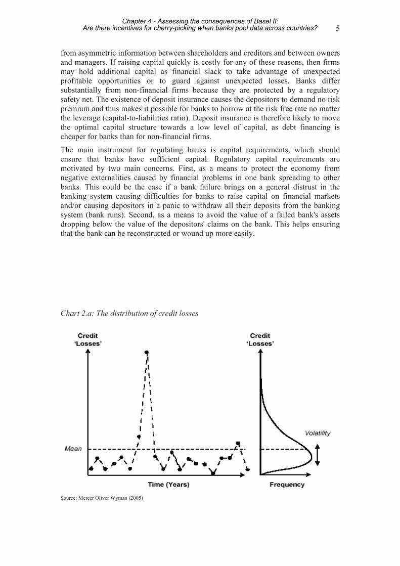
5

from asymmetric information between shareholders and creditors and between owners and managers. If raising capital quickly is costly for any of these reasons, then firms may hold additional capital as financial slack to take advantage of unexpected profitable opportunities or to guard against unexpected losses. Banks differ substantially from non-financial firms because they are protected by a regulatory safety net. The existence of deposit insurance causes the depositors to demand no risk premium and thus makes it possible for banks to borrow at the risk free rate no matter the leverage (capital-to-liabilities ratio). Deposit insurance is therefore likely to move the optimal capital structure towards a low level of capital, as debt financing is cheaper for banks than for non-financial firms.

The main instrument for regulating banks is capital requirements, which should ensure that banks have sufficient capital. Regulatory capital requirements are motivated by two main concerns. First, as a means to protect the economy from negative externalities caused by financial problems in one bank spreading to other banks. This could be the case if a bank failure brings on a general distrust in the banking system causing difficulties for banks to raise capital on financial markets and/or causing depositors in a panic to withdraw all their deposits from the banking system (bank runs). Second, as a means to avoid the value of a failed bank's assets dropping below the value of the depositors' claims on the bank. This helps ensuring that the bank can be reconstructed or wound up more easily.

Chart 2.a: The distribution of credit losses

Source: Mercer Oliver Wyman (2005)


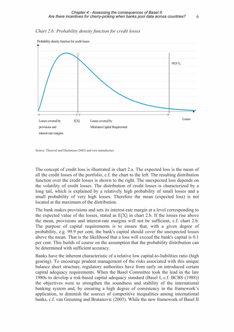
6

Chart 2.b: Probability density function for credit losses

Losses

Probability density function for credit losses

Losses covered by

provisions and

interest-rate margins

Losses covered by

Minimum Capital Requirement

99,9 %

E[X]

Source: Thoraval and Duchateau (2003) and own manufacture

The concept of credit loss is illustrated in chart 2.a. The expected loss is the mean of all the credit losses of the portfolio, c.f. the chart to the left. The resulting distribution function over the credit losses is shown to the right. The unexpected loss depends on the volatility of credit losses. The distribution of credit losses is characterized by a long tail, which is explained by a relatively high probability of small losses and a small probability of very high losses. Therefore the mean (expected loss) is not located at the maximum of the distribution.

The bank makes provisions and sets its interest-rate margin at a level corresponding to the expected value of the losses, stated as E[X] in chart 2.b. If the losses rise above the mean, provisions and interest-rate margins will not be sufficient, c.f. chart 2.b. The purpose of capital requirements is to ensure that, with a given degree of probability, e.g. 99.9 per cent, the bank's capital should cover the unexpected losses above the mean. That is the likelihood that a loss will exceed the bank's capital is 0.1 per cent. This builds of course on the assumption that the probability distribution can be determined with sufficient accuracy.

Banks have the inherent characteristic of a relative low capital-to-liabilities ratio (high gearing). To encourage prudent management of the risks associated with this unique balance sheet structure, regulatory authorities have from early on introduced certain capital adequacy requirements. When the Basel Committee took the lead in the late 1980s to develop a risk-based capital adequacy standard (Basel I, c.f. BCBS (1988)) the objectives were to strengthen the soundness and stability of the international banking system and, by ensuring a high degree of consistency in the framework’s application, to diminish the sources of competitive inequalities among international banks, c.f. van Greuning and Bratanovic (2003). While the new framework of Basel II


7

aims to provide a comprehensive approach to measuring banking risks, its fundamental objectives remain the same as those of the 1988 Accord.

3. Basel II This section reviews the Basel II framework and describes the calculation of the minimum capital requirements using the internal ratings-based approaches. Furthermore, the Basel II minimum requirements for estimation of probability of default as well as the Basel II requirements and other guidelines on data pooling are discussed. Finally, we compare our approach to the requirements and guidelines.

3.1 IRB approach of the Basel II framework In June 2004 the central bank governors and the heads of banking supervisory authorities of the G10 countries (the Basel Committee of Banking Supervision) endorsed the Revised Framework for Capital Measurement and Capital Standards, also known as Basel II, which is a set of recommendations for the capital requirements imposed on banking organizations by supervisory authorities. Basel II is designed to cope with the shortcomings of the current regime, the 1988 Capital Accord, c.f. Caruana (2004a) and Caruana (2004b).

The 1988 Capital Accord states that banks should hold capital in excess of 8 per cent of the risk weighted assets for credit risk and market risk. The Basel Committee of Banking Supervision introduced the Accord as a set of capital adequacy rules to apply for major internationally active banks based in the G10 countries. A common set of rules was necessary to prevent bank failures and at the same time ensure level playing field for banks competing in the same countries. Following the introduction of the Accord more than 100 countries including the EU chose to adopt the 1988 Accord for their banks.

The Basel Committee has made it clear, that Basel II aims at the same overall global capital requirement as the 1988 Accord, but to make each individual bank's capital requirement more closely linked to its risk of economic loss.

More than 100 countries worldwide are expected to adopt Basel II, c.f. BIS (2004) and Keefe (2004). The European Commission has worked in parallel with the Basel Committee on proposals for directives to replace the 1988 Accord with Basel II in the EU countries for credit institutions and investment firms. On 14 July 2004 the European Commission presented its proposals for Directives to transpose the Basel II into European Law. The proposed directives are expected to be finally adopted by the European Parliament and the Council in 2005 and enter into force at end-2006. Credit institutions and investment firms can apply the existing capital-adequacy rules until end-2007. However, institutions applying for the most advanced approaches8 for calculation of minimum capital requirements may not apply the new rules until 2008.

Basel II consists of three pillars. Pillar I sets out criteria for banking organizations' calculation of minimum capital requirements to cover market risk, credit risk and operational risk. The latter was not covered by the 1988 Accord. Pillar 1 represents an extension of the requirements in the 1988 Accord and introduces more sophisticated calculation approaches, which aligns the minimum capital requirements more closely

8 The advanced internal ratings-based approach for credit risk and advanced measurement approach for

operational risk


8

to the banks' risk of economic loss, especially for credit risk. For credit risk the banks can with the approval of the supervisory authority choose one of three approaches, namely the standard approach, the foundation internal ratings-based approach and the advanced internal ratings-based approach. In the two sophisticated approaches, the internal ratings-based approaches (IRB), the banks use their internal credit-scoring models in the calculation of the capital requirement, c.f. below. Pillar II requires banks to assess their need for capital in relation to their overall risk profile including risks not or only partly covered by pillar I, e.g. interest-rate risk on the banking book, business risk and strategic risk. Furthermore, the supervisory authority must evaluate the banks' assessment of its capital need. Pillar III sets out principles for banks' disclosure of information concerning risks and capital to enhance market discipline.

The focus of this paper is on the foundation IRB-approach for calculation of the capital requirement for credit risk of exposures to small and medium sized enterprises (SME) under pillar I. Nonetheless we will briefly review the main features of both the foundation IRB approach and the advanced IRB approach.

Both approaches use four quantitative inputs: 1) the probability of default (PD), which measures the likelihood that a borrower will default over a one-year time horizon, 2) loss given default (LGD), which measures the proportion of the exposure that will be lost if a default occurs, 3) exposure at default (EAD), which measures the nominal value of the debt and 4) the effective maturity (M), which measures the remaining economic maturity of exposure. Risk weights are calculated by inserting PD, LGD and M into the formulas prepared by the Basel Committee. The minimum capital requirement (K*) for each exposure can then be calculated as 8 % of the risk weight (RW) multiplied by EAD:

EADRWK ××= 08.0*

The main difference between the foundation and the advanced IRB approach is the extent the approaches rely on inputs provided by credit institutions on the basis of their own estimates, as opposed to those inputs that are pre-specified by the supervisor. In the foundation IRB approach, only the PDs are estimated by the credit institutions, whereas, in the advanced IRB approach, the credit institutions estimate all four risk factors themselves.

Under the IRB approaches, banks must categorize credit exposures into the following broad classes: corporate, sovereign, bank, retail and equity. For corporate exposures banks are permitted to distinguish separately exposures to SMEs and give them a lower risk weight. SMEs are defined by their size as corporate exposures where the reported sales for the consolidated group of which the firm is a part is less than 50 million euro. A firm-size adjustment is made to the corporate risk weight formula for exposures to SMEs. Very small exposures to SMEs can under certain conditions be eligible for the more favourable retail treatment. For an SME to be treated as a retail exposure it needs to have its loans managed as other retail exposures and the total exposure of a bank to an individual firm has to be less than 1 million euro. For the interested reader the Basel II formulas for calculation of credit exposures to SMEs are presented in appendix 1.

In this paper the calculations of minimum capital requirements for credit risk for SMEs are based on estimates of PD's from a credit-scoring model. We apply the foundation IRB approach which prescribes LGD=45 % and M=2.5 years for corporate


9

exposures. EAD is calculated as the sum of loans and long-term debt9. We assume that exposures are without collateral. SMEs are defined as corporate exposures where the reported sales of the firms are between 1 and 50 million euro. In this paper we do not consider the more favorable retail treatment for the very small SMEs with exposures less than 1 million euro. That is, we apply the SME formula for all firms in the data set.

3.2 Basel II requirements for estimation of probability of default For supervisory authorities to approve a bank for one of the IRB approaches for calculation of the minimum capital requirement for credit risk, the bank must demonstrate that it fulfills a number of requirements on an ongoing basis. This section describes the minimum requirements in Basel II, which are of particular importance when estimating probability of defaults, and it compares these requirements to the data and method we apply for calculating minimum capital requirements. According to Basel II default has occurred when 1) the bank considers that the obligor is unlikely to pay its credit obligations to the bank, the parent undertaking or any of its subsidiaries in full without recourse by the bank to actions such as realizing security, or 2) the obligor is past due more than 90 days on any material credit obligation to the bank, the parent undertaking or any of its subsidiaries. Basel II lists a number of indicators for the bank's assessment of an obligor's unlikeliness to pay. These include situations where the bank puts the credit obligation on non-accrued status, makes a value adjustment resulting from a significant perceived decline in credit quality, sells the credit obligation at a material credit-related economic loss, consents to a distressed restructuring of the credit obligation likely to result in diminished financial obligation, has filed for obligor's bankruptcy or where the obligor has sought or has been placed in bankruptcy. The same definition is used in the EU directive proposal. Of the two complementing approaches for defining default, the suggested indicators for the banks' assessment of the obligor's unlikeliness to pay (approach 1) imply that in most cases default will occur before the obligor is 90 days past due (approach 2). According to the EU directive proposal until 2012 the 90-days may be extended up to 180 days if local conditions make it appropriate, c.f. European Commission (2004: article 154, 4). The bank must have a rating system of its obligors with a meaningful distribution of exposures across grades with minimum 7 rating grades for non-defaulted obligors and one for defaulted obligors. For each grade the bank must estimate a PD for all the obligors in that grade. The EU directive proposal relaxes this requirement and allows banks to use direct estimates of PDs for calculation of the capital requirement, i.e. without introducing a rating system, c.f. European Commission (2004: Annex VII, part 4, 4). This implies that each obligor has a separate PD, whereas, when using a rating system, the obligors of each rating grade have the same PD. According to Basel II the PD should be a long run average of one-year default rates. The length of the underlying historical period should be at least five years. In the EU 9 According to Basel II, with the foundation internal ratings-based approach, EAD should be calculated as the on

and off-balance sheet position gross of specific provisions or partial write-offs, c.f. BCBS (2004:66).


10

directive proposal, the requirement for the underlying historical period is cut down to two years until end-2007, increasing by one year per year thereafter until end-2010, c.f. European Commission (2004:article 154,4). Therefore, the end-requirement will be an underlying period of five years as in Basel II. Basel II requires banks to use information and techniques that take appropriate account of the long-run experience when estimating the average PD for each rating grade. The EU directive proposal allows banks to use direct estimates of PDs without introducing a rating system. Nevertheless, we expect that these estimates should also take appropriate account of the long-run experience. The number of exposures in the sample and the data period used for quantification has to be sufficient to provide the bank with confidence in the accuracy and robustness of its estimates. In order to avoid over-optimism, a bank must add to its PD-estimates a margin of conservatism. If methods and data are less satisfactory and the likely range of errors is larger, the bank has to use a larger margin of conservatism. Finally, Basel II emphasizes that human judgment and human oversight is necessary to ensure that all relevant information, including that which is outside the scope of the model is also taken into consideration, and that the model is used appropriately. In addition, banks must recognize the importance of judgmental considerations in combining results of techniques and in making adjustments for limitations of techniques and information. For the purpose of this paper we estimate the probability of default for firms using a credit-scoring model. In line with the EU directive proposal, we estimate probability of default directly for each firm without developing a rating system and assigning firms to risk grades. Introducing a rating system would be more in line with Basel II, but would on the other hand force us to make a number of assumptions (e.g. definition of rating grades and calculation of average probability of defaults) bringing in unnecessary noise, which would blur our results. Furthermore, we apply the model's estimation of credit scores directly as probability of defaults. This implies no use of human judgment concerning probability of default for each firm or adding a conservative margin to avoid over-optimism. Use of human judgment and adding a conservative margin is not relevant for our problem since this would imply a shift in the PDs in the same direction for PDs obtained both from the estimation of the single-country credit-scoring models and from the multi-country credit-scoring models. The estimations of the credit-scoring models in this paper cover only firms that have handed in financial statements in the period 2000 – 2002. It is important to note that the correct computation of minimum capital requirements, according to Basel II, demands that the underlying historical period must be at least five years. The estimated probability of default in this paper does not take this requirement into account. However, it does accommodate the requirements in the EU directive proposal, in which the underlying historical period is reduced to two years and increasing one year per year from end-2007 to end-2010. This means that in a transition phase it is sufficient to use the data available to us.


11

The focus in this paper is on the firms that go bankrupt. This “financial distress-event” is a fairly late credit event compared to the Basel II definition. As this model is based on public information only, it is not possible to follow the Basel II default definition. Several studies imply that this is not of significant importance, when building the credit-scoring model. Hayden (2003) shows that credit-scoring models that rely on bankruptcy as default criterion instead of delay-in-payments can be equally powerful in predicting the credit loss events. Furthermore, Moody’s Investors Service (2001) reports that experience shows that the factors that can predict default are generally the same, no matter whether the definition of default is 90 days past due or bankruptcy. It is not uncommon to use a fairly late credit event in academic studies. The definition of default used in two of the three studies mentioned in the introduction is the bankruptcy event (Saurina and Trucharte (2003) and Masschelein (2003)). The last study uses banks' classification of loans as bad loans (Fabi, Laviola and Reedtz (2004)). Though using the Basel II default definition is not essential for building credit-scoring models in general, it is of importance when the probability of defaults estimated in the credit-scoring model is used for calculating the level of the capital requirement – since it affects the level of the PD and hence the resulting capital requirement. For the purpose of this paper, which compares the capital requirements using single-country credit-scoring models and multi-country credit-scoring models and the incentive structures this might create, the absolute level of the calculated capital requirements is not important.

3.3 Data pooling – requirements and guidelines Basel II and the EU directive proposal both allow banks to pool data to overcome their data shortcomings. The emergence of a number of data pooling projects illustrates the considerable need for banks to pool data in order to fulfill the Basel II IRB requirements. This section describes Basel II's and the EU directive proposal's requirements with regard to data pooling and furthermore it highlights recommendations on data pooling from guidelines published by supervisory authorities. Finally, these requirements and guidelines are compared to the data and method we apply for calculating minimum capital requirements. Basel II allows for banks to pool internal data with external data, c.f. BCBS (2004:92ff). The bank has to demonstrate that the internal rating systems of other banks in the pool are comparable to its own and representative of the population of the bank's actual borrowers. Furthermore, estimates based on internal or external data should be representative of long-run experience. The Basel Committee does not give specific recommendations on the setting up and use of pools, e.g. the use of cross-country pools - for instance for a bank with exposures in different countries (like our hypothetical bank) or for a bank with data for one country who plans to pool this with banks who have data from other countries. The EU directive proposal elaborates on the requirements for using external and pooled data. The directive proposal states that credit institutions using external data that is not itself consistent with the definition of default shall demonstrate that appropriate adjustments have been made to achieve broad equivalence with the definition of default, c.f. the European Commission (2004, Annex 7, part 4, 46). In addition, a credit institution using data pooled across credit institutions has to


12

demonstrate that the pool is representative for the portfolio for which the pooled data is used and that the pooled data is used consistently over time by the credit institution for its permanent estimates, c.f. the European Commission (2004, Annex 7, part 4, 57). The directive proposal requires that credit institutions use internal data for assigning exposures to rating grades as the primary source of information when estimating PDs and LGDs. Credit institutions are permitted to use external data (including pooled data) for quantification provided a strong link can be demonstrated between 1) the credit institution's process for assigning exposures to grades and the process used by the external data source and 2) the credit institution's internal risk profile and composition of the external data, c.f. the European Commission (2004, Annex 7, part 4, 69). That is, the pooled data should be representative for the credit institution's loan portfolio. The directive proposal does not provide rules on the use of external data or pooled data when using direct PD-estimation, i.e. estimating PD's without using rating grades. The wording of the directive proposal with regard to the use of external data and data pooling can be interpreted as applying for data pooling between banking institutions, which are a part of the same banking group, as well as for one bank wishing to pool data with other banks. The rules would thus apply for our hypothetical bank with cross-country exposures and for a bank planning to pool data with banks in other countries. Published guidance on the use of pooled data for PD-estimation is very limited or kept in general terms. Oesterreichische Nationalbank (2004:63ff) highlights the importance of a uniform definition of default in the pooled data and points out, that discrepancies can arise between individual countries due to use of different accounting standards. In this paper we use a uniform definition of default. The default observations are constructed as firms exiting the Amadeus database due to bankruptcy. As the three countries (France, Italy and Spain) are countries with French-civil-law tradition, differences between the institutional frameworks are limited, c.f. La Porta, Lopez-De-Silanes, Shleifer and Vishny (1998), who scores the countries based on enforcement variables (e.g. efficiency of judicial system), accounting standards and creditor rights (e.g. no automatic stay on assets and secured creditors paid first). Furthermore, the Amadeus database harmonizes accounting data from different countries. Discrepancies due to the use of different accounting standards are thus very limited. The UK Financial Services Authority (UK FSA) states in their consultation paper that if a bank uses data pooled across institutions it should be able to demonstrate to the FSA, that the pool is representative for the portfolio for which the pooled data is used, c.f. UK FSA (2005, appendix 1). This statement could apply both for a bank operating in other countries through subsidiaries, which plans to pool data from the subsidiaries and the parents, and for a bank planning to pool data with banks based in other countries. The consultation paper does not elaborate on the definition of representativity. The EU Committee of European Banking Supervisors is also working on guidelines on the implementation, validation and review of the IRB approaches including guidelines on the use of data pooling. These guidelines are not yet published.


13

Our hypothetical bank pools data on SME exposures in France, Italy and Spain. Based on this data set (portfolio) we estimate statistical default prediction models, namely three different hazard models, c.f. section 5. As we control for a number of effects in the estimations, e.g. industry, size, age and legal form (see section 5), we do not need to ensure that our sample from France is representative of the sample from Spain and Italy etc. In fact, even if there were no firms in the manufacturing sector in France, it would not matter for the estimation of the probability of default, as the dummy, which indicates whether a specific company is a manufacturing company or not, would then be set to 0, when the PDs for France are estimated. In the same way, it would not matter if there, for example, were no public limited liability companies in Spain. In the actual estimations, the estimated PD for each individual firm includes information on a wide number of individual characteristics, and so all of these characteristics are taken into consideration, when the credit-scoring models are estimated. Even though it is not necessary to show that all industries, sizes and legal forms are present for each country in our sample in order to get consistent estimates, c.f. above, for the interested reader, table 3.3 shows that in each of the countries we are analyzing the same industries, sizes and legal forms are present (further details on data are given in section 4). There are differences between the number of firms in the different industries, sizes and legal forms in the respective countries, but as is explained above, it is not a problem in our setting. Table 3.3: The analyzed sample split up on legal form, size and industries (percentages in brackets)

Spain France Italy

Public limited liability company

46,317 (62 pct.) 89,314 (86 pct.) 31,312 (32 pct.)

Legal form (number of firms) Private limited

liability company 28,635 (38 pct.) 14,530 (14 pct.) 65,129 (68 pct.)

Mean 8.51 8.45 8.61 Size (measured as ln(total assets)) Median 8.35 8.30 8.50

Farming, forestry and fishing

1,616 (2 pct.) 1,284 (1 pct.) 443 (0 pct.)

Mining 905 (1 pct.) 858 (1 pct.) 722 (1 pct.)

Manufacturing 26,648 (36 pct.) 31,829 (31 pct.) 50,861 (53 pct.)

Energy 389 (1 pct.) 275 (0 pct.) 285 (0 pct.)

Construction 8,945 (12 pct.) 8,808 (8 pct.) 7,298 (8 pct.)

Trade and hotel 21,554 (29 pct.) 35,714 (34 pct.) 25,215 (26 pct.)

Transport 4,578 (6 pct.) 6,113 (6 pct.) 3,789 (4 pct.)

Business service 7,176 (10 pct.) 14,244 (14 pct.) 4,958 (5 pct.)

Public service activities

1,022 (1 pct.) 2,380 (2 pct.) 1,233 (1 pct.)

Industries (number of firms)

Organisations 2,119 (3 pct.) 2,339 (2 pct.) 1,317 (1 pct.)


14

In the case where the estimated model does not include a large number of explanatory variables, e.g. only a few accounting ratios, the user of the model would need to ensure that the same sectors are represented in the various portfolios, which are pooled, just as well as it would be a good idea to ensure, that the composition of the portfolio with respect to legal form, would be the same across portfolios. Concerning both variables (sector affiliation and legal form), a number of credit-scoring studies have documented that the probability of default differs across sectors, as well as across legal form, see e.g. Dyrberg (2004).

4. Data The data used for Italy, Spain and France comes from the Amadeus database, which is a pan-European database provided by Bureau van Dijk. This section presents the data set and explains the construction of the dependent variable. Furthermore, this section gives an overview of the sample selection criteria and it presents the hypothetical loan portfolio. For further details on the data set the reader is referred to Rommer (2005a). 4.1 The raw data The Amadeus database comprises information on financial issues as well as non-financial issues. Bureau van Dijk has harmonized the database so that the financial items across countries are comparable. As part of the non-financial information, the database entails a legal status variable. This variable contains information on the status of the firm (active, bankrupt etc.). This piece of information is particularly important for this study, as it is used to construct the dependent variable. Unfortunately, information on the legal status variable is only kept in the database for 3 years, and so, currently, the estimations of the credit-scoring models cover only firms that have handed in financial statements in the period 2000 – 2002. Ideally, the estimation period would have covered a full business cycle. In the dataset, firms that hand in a financial statement in 2000 are recorded as belonging to year 2000. Firms that hand in a financial statement in 2001 are recorded as belonging to year 2001 etc. Some firms are represented with one data point, e.g. in 2000, in 2001 or in 2002, other firms will be represented by two points, e.g. in 2000 and 2001 or in 2001 and 2002, and other firms will be represented by three data points. In technical terms, the firms are both flow and stock sampled and the length of the spells varies across firms. There is one spell for each firm. When a firm has left the sample, it can never re-enter, i.e. the exit event is an absorbing state. For further details on duration data, the reader is referred to Dyrberg (2004). 4.2 Construction of the dependent variable The legal status variable for constructing the dependent variable, which is the event “financially distressed firms”, i.e. a measure of the firms that may inflict a loss on the financial sector. In the Amadeus database it is registered whether or not the company is bankrupt (France, Italy, Spain), whether or not the company is in receivership (France), and whether or not it has defaulted on its payments (Spain, France). The broadest measure of financial distress, which can be used here, is therefore a measure, which, for each country, includes the events that are registered for the respective countries. This broad measure is not a satisfactory measure for financial distress in this set up, where the impact on the calculated capital requirements of the estimation of single-country credit-scoring models and multi-country credit-scoring models is at


15

focus. Therefore, in order to make the financial distress event consistent across countries, we include only bankrupt firms for the measure of financial distress in the analyzed hypothetical loan portfolio. Accordingly, a hypothetical loan portfolio is constructed, which only includes the firms that go bankrupt and active firms. 4.3 Sample selection criteria and the hypothetical loan portfolio In order to construct the hypothetical loan portfolio, various sample selection criteria, which are discussed in details in Rommer (2005a), are applied to the data. Table 4.a gives an overview of the applied criteria. In particular, note that the analysed sample only includes SMEs with annual sales less than 50 million euro to comply with the criteria for when a firm can be treated as SME using the IRB approach. After the application of the sample selection criteria, the hypothetical loan portfolio is constructed. Table 4.b shows the hypothetical loan portfolio, i.e. the number of observations in the sample, which are used in the estimations (with bankruptcy as a default criterion). From the table we can see that our particular hypothetical bank has experienced most bankruptcies in its French portfolio (597 bankruptcies are registered) and the smallest number of bankruptcies in Spain (115 bankruptcies are registered).

Table 4.a: Sample selection criteria Criteria

Only unconsolidated statements are analysed

Financial institutions and non-financial holding companies are excluded

Only public limited liabilities and private limited liabilities are analysed

Only SMEs with at least 10 employees and with total assets of at least 2 million euro. This criterion ensures that micro-companies, which resemble households, are excluded from the sample, and furthermore, that only “truly” active companies are considered, c.f. the discussions in Rommer (2005a)

SMEs with total annual sales less than 50 million euro

Conceptual

Some firms leave with no explanation (that is, they are not assigned an exit code). These firms are called attritioners. Based on the analysis in Rommer (2005a), they are excluded from the dataset

Active companies are excluded if they hand in a financial statement in 2000 and 2002 only.

Various corrections are made to the database (e.g. firms with illogical variables, such as short-term debt less than zero and a solvency ratio larger than 100 pct., are excluded).

Firms with missing variables on any of the explanatory variables are excluded.

Other

If a company hands in two financial statements in one year, only the last financial statement is included in the estimations.


16

Table 4.b: Bankrupt firms and other firms (period covered 2000-2002) Spain France Italy Pooled

Number of firm-years

In percent of total


In percent of total


In percent of total


In percent of total

Bankruptcy 115 0.15 597 0.57 155 0.16 867 0.32

Active and censored firms

74837 99.85 103247 99.43 96286 99.84 274370 99.68

Total 74952 100 103844 100 96441 100 275237 100

5. Estimation of the PDs This section gives an overview of how the PDs are estimated, including the explanatory variables that are used in the estimations. Based on the dataset presented in table 4.b, accounting-based credit-scoring models are estimated. An accounting-based credit-scoring model is based on information extracted from company accounts and in some cases also non-financial information (such as the age of the company). It estimates the probability that a particular firm will default on its debt obligations. Various estimation techniques have been suggested in the accounting-based credit-scoring literature (e.g. discriminant analysis and logistic regression).10 Here the estimation strategy of Shumway (2001) is followed, thus the credit-scoring models are estimated as hazard models. The hazard functions are specified as logit models. The firms that exit for other reasons than financial distress (i.e. firms that are voluntarily liquidated) are treated as censored or no longer observed when they leave the dataset. Three different credit-scoring models are estimated: First, individual credit-scoring models for each country are estimated. Second, a multi-country credit-scoring model with country dummies is estimated. Third, a multi-country credit-scoring model without country dummies is estimated. The explanatory variables, which are included in the estimations, can be seen from table 5. They are divided into three categories: Core variables, proxies and controls. For further details the reader is referred to Rommer (2005a), which uses the same data. 10 For an overview of the literature the reader is referred to Jones (1987), Dimitras, Zanakis and Zopounidis

(1996), Altman and Saunders (1998), Balcaen and Ooghe (2004) and Lando (2004). Some of the often-quoted accountings-based credit-scoring studies are Beaver (1966), Altman (1968), Ohlson (1980) and Shumway (2001).


17

Table 5: The explanatory variables Variable

Profitability: Earnings ratio= EBITDA/total assets. EBITDA = earnings before interest, taxes, depreciation and amortization Solvency: Solvency = Equity/total assets Leverage: Loans/total assets Firms size: Ln(total assets)

Core variables

Age: The year of the financial statement minus the year of incorporation Legal form: This dummy is equal to 1, if it is a private limited liability company, and equal to 0, if it is a public limited liability company. Independence indicator: Three dummies are included. One is equal to one when the ownership is very concentrated (when at least one of the shareholders has an ownership above 49.9 pct.). One is equal to one when the ownership is of medium concentration (when none of the shareholders have an ownership percentage above 49.9 pct, but at least one or more shareholders has an ownership percentage above 24.9 pct.). One is equal to one when the ownership is not so concentrated (when none of the shareholders has more than 24.9 pct. of ownership share). Reference category is all other firms (for which there is no information on the shareholders). Shareholders: This variable measures the number of recorded shareholders.

Proxies

Subsidiaries: This variable measures the number of subsidiaries that a company has registered. Sector affiliation dummies: The data is divided in the following industries: 1) Farming, Forestry, Fishing 2) Mining, 3) Manufacturing, 4) Energy, 5) Construction, 6) Trade and hotel, 7) Transport, 8) Business service, 9) Public service activities, 10) Organisations etc. Financial firms and holding companies are excluded from the analysis. As there are no NACE codes for the IT and tele-sector a (self-constructed) IT and tele-dummy is included in the estimations. On top of belonging to one of the above sectors a firm is considered to by in the IT and tele group if it has activities in one of the sectors listed in table 14.b in section 14 in Rommer (2005a). Further details on the sectors are found in table 14.a in section 14 in Rommer (2005a). Note that in the actual estimations the following industries are grouped (as the data are too sparse otherwise): Organisations and public service activities are grouped. Farming, forestry, fishing, mining and energy are grouped.

Controls

Macroeconomic environment: Year dummies are included to control for business cycle effects. The reference year is 2000. Two dummies are included. One is equal to 1 for the firms, which hand in their financial statements in 2001. One is equal to 1 for the firms, which hand in their financial statements in 2002.

Controls (only in the multi-country credit-scoring model with country dummies)

Country dummies: A dummy for each country is included in the estimations to control for country-specific effects.

Source: Rommer (2005a) and own manufacture

6. Results Based on data on SMEs in Italy, Spain and France we have constructed a hypothetical loan portfolio. We have applied single-country credit-scoring models and multi-country credit-scoring models with and without country dummies to estimate PDs. The PDs have been used to calculate the resulting minimum capital requirement for our hypothetical bank using the foundation IRB approach.


18

Table 6: A comparison of the capital requirements for the hypothetical bank using the companies that were active in 2002 in the three model set ups, in million euros, and the largest range in capital requirements in percent of the smallest capital requirement (right column) Single-country

models Multi-country model (with country dummies)

Multi-country model (without country dummies)

Largest range in capital requirements in percent of the smallest capital requirement

IT 94,703 99,323 139,654 47 ES 122,588 109,837 148,737 35 FR 100,034 104,489 81,883 27 Total 317,324 313,649 370,274 18 Note: The number of active companies in 2002 is 35,818 in Italy, 29,447 in Spain and 41,251 in France. The total number of active companies in the three samples is 106,516.

This section presents the resulting capital requirements calculated on the basis of the PDs estimated in the single-country credit-scoring models and the multi-country credit-scoring models with and without country dummies, c.f. appendix 2, table 6 and figure 6. The estimated probabilities of default are set into the formulas for calculating the capital requirements using the foundation IRB approach for SMEs. In the formulas loss given default (LGD) is set to 45 pct. and maturity (M) is taken as 2.5 as prescribed by the foundation IRB approach. The exposure at default (EAD) is calculated as the sum of loans and long-term debt.11 12

The results presented in table 6 (further details are found in appendix 2) show that for each country the difference in the calculated capital requirements is quite large, when the probability of default is estimated using a single-country credit-scoring model compared to using multi-country credit-scoring models (with or without country dummies). Particular different results are obtained from the single-country credit-scoring models and the multi-country credit-scoring model without country dummies, and between the multi-country credit-scoring model with country dummies and the multi-country credit-scoring model without dummies, c.f. table 6. It is remarkable how limited the differences in the calculated capital requirements are between the single-country and the multi-country credit-scoring models with country dummies.

It is particularly noticeable that the lowest capital requirement in the countries is obtained using different model set-ups. In the Italian case, estimating a single-country credit-scoring model delivers the lowest capital requirement, in the Spanish case a multi-country model with country dummies delivers the lowest capital requirement and in the French case the multi-country model without country dummies delivers the lowest capital requirement. In the Italian and Spanish case the multi-country model without country dummies delivers the highest capital requirement, whereas the multi- 11 In the Amadeus database liabilities are spit up on current liabilities (short-term) and non-current liabilities

(long-term). Current liabilities are divided into loans, creditors and other current liabilities. Non-current liabilities are divided into long-term debt and other non-current liabilities (incl. provisioning).

12 A firm can have several bank connections. It is not indicated in the Amadeus database, whether the firms use one or more than one bank connection. In the calculations total exposure of a firm is interpreted as the exposure to one hypothetical bank.


19

country model with country dummies delivers the highest capital requirements in the French case.

In the situation where a bank considers pooling data with banks from other countries, the bank has an incentive to choose the method, which delivers the lowest capital requirement without considering what level of capital is actually appropriate to cover the overall credit risk, i.e. cherry-picking. Note, however, that Basel II does not allow banks to change their model for estimation of PD every so often for instance in order to obtain the lowest possible minimum capital requirement. Basel II states that banks must monitor the model stability, c.f. BCBS (2004:86). The EU directive proposal furthermore requires banks to validate the accuracy and consistency of rating systems, processes and the estimation of all relevant parameters, and points out that changes in estimation methods and data shall be documented, c.f. European Commission (2004:appendix VII, part 4, 109 and 112).

Table 6 shows that a bank with exposures to Italian firms would benefit form choosing a single-country model, a bank with the exposures to Spanish firms would benefit from using the multi-country model with country dummies etc. Furthermore, table 6 illustrates that our hypothetical bank would obtain the lowest capital requirement from estimating a multi-country model with country dummies. The overall capital requirement would then be marginally lower (313,649 million euro) compared to estimating single-country credit-scoring models (317,324 million euro) and much lower compared to a multi-country credit-scoring model without country dummies (370,274 million euro).

Chart 6: Capital requirements over total exposure at default (EAD), split up on country and method

0

0,5

1

1,5

2

2,5

3

3,5

4

4,5

5

IT ES FR Total

Single-country models Multi-country model (with country dummies)

Multi-country model (without country dummies)

Pct


20

Chart 6 illustrates the capital requirement over total exposure at default (EAD), split up on country and method. As we normalize the capital requirements in each country with the total exposure at default in each country, the figure enables us to compare the riskiness of the exposures across countries. The chart shows that the French loan portfolio is more risky (in the sense that it has a higher capital requirements over EAD), and that the Italian and Spanish loan portfolios are at the same risk-level, when the two preferred methods are compared. As we would expect, the total loan portfolio, which consists of exposures to all countries, is placed somewhere in between the French, and the Italian and Spanish loan portfolios.

The differences in the calculated capital requirements are not due to differences in the default definition, as only bankrupt firms from countries with French-civil-law tradition were considered. However, it can be sensitive towards the way we constructed the default measure. As was noted in section 4.2, the broadest measure of financial distress, which could be used, is a measure, which, for each country, includes the events that are registered for the respective countries. In order to make the default definition comparable across countries, we chose, in this paper, only to focus on bankruptcies. It is also worth pointing out that we used a database, which was harmonized across countries, and that we controlled for a number of variables in the estimations, including age of the company, size, solvency ratio, leverage, profitability, legal form, ownership variables and sector affiliation.

The calculations in this paper are based purely on the quantitative and technical requirements of the foundation IRB approach of Basel II and the EU directive proposal. We do not take into consideration effects of applying human judgment and a conservative perspective on PD estimation. The example of our hypothetical bank serves to illustrate the purely technical consequences of pooling data and the incentives it might give for banks when calculating minimum capital requirements.

One reason why the calculated capital requirements are different in the countries depending on whether the single-country or a multi-country model (with or without country dummies) is estimated could be that the predictors of financial distress differ across countries, c.f. box 6. As we controlled for macroeconomic effects by the use of year dummies, c.f. section 4, the differences in the predictors of financial distress in the single-country models are not due to differences in the macroeconomic environment in the respective countries, i.e. different levels of the real interest rate, growth, inflation etc. Note, however that differences in the macroeconomic environments could have the implication that the number of firms in financial distress differ across countries.

The concrete implication for banking supervision from the analysis is that banks and supervisory authorities must be aware that the pooling of data from several countries should be done with caution. As there are not many official guidelines from authorities on the issue, we believe that the illustration in this paper of the consequences of pooling data from several countries serves as an important input to the debate on how to set up credit-scoring models in banks that have cross-border exposures as well as for banks who choose to pool their data with banks in other countries. We have shown that it is not enough for banks to apply similar definitions of default and similar accounting regimes in the countries. Banks and regulators should also have a careful look into the models, especially the factors that drive financial distress, e.g. along the lines of Rommer (2005a). Rommer (2005a) is one concrete example of an econometric study that investigates the determinants of


21

financial distress in several countries. However, it is not only important to assess the factors that drive financial distress. Credit institutions and regulators should also pay special attention to 1) the sample selection and design, 2) the statistical technique and 3) the evaluation of results.

Under item 1) one issue, which is important to assess, is the extent of drop-outs in the credit institutions portfolio. Our analysis is based on a panel data set. In our observation window, which spans from 2000 to 2002, we follow the firms from the time, when they are incorporated, till they leave the sample. This is not always the case for individual credit institutions, c.f. Rommer (2005b). Credit institutions may experience drop-outs for a number of reasons, e.g. a firm may choose another bank as it offers a better service or a better price, or e.g. because the specific firm is asked to leave its current bank, as it suspects that it is heading into financial distress. It is important that the drop-outs are carefully analyzed in order to find out what kind of drop-outs one deals with. Otherwise inconsistent estimates may be obtained, when the credit-scoring model is set up and estimated. Another issue, which also falls under item 1), is the reject inference problem: In Basel II it is stated that internal ratings and default and loss estimates must play an essential role in the credit approval process. It is important to be aware, that if the “models estimated using data on already approved applicants are applied to all applicants, then a sample selection bias is introduced”, c.f. Rommer (2005b). The problem is that if only obligors, who have already been approved for a loan, are taken into account then it is not appropriate to use the same model to consider new applications. In the academic literature this problem is called the reject inference problem.

Concerning item 2), which is the choice of statistical technique, a wide range of papers discuss the differences between the various techniques, which have been suggested in the literature. The standard credit-scoring methods are multivariate discriminant analysis, logistic regression and hazard models. These methods are discussed in Altman (1968), Ohlson (1980) and Shumway (2001), respectively. It is important that credit institutions and regulators are aware of the advantages and limitations of the chosen approach. Examples of papers, which discuss various methodological aspects, are Dyrberg (2004), Rommer (2005b), Rommer (2005c), Altman, Marco and Varetto (1994), Back, Laitinen, Sere and Wezel (1996), Begley, Ming and Watts (1996) and Frydman, Altman and Kao (1985).

Concerning the evaluation of results (item 3) credit institutions have to show that their models have discriminatory power, i.e. that the models can discriminate between defaulting and non-defaulting borrowers. In the credit-scoring literature it is common to report the type I errors (missing prediction, i.e. the model predicts a non-event, but it turns out to be an event) and type II errors (wrong signal, i.e. the model predicts an event, but it is a non-event). A good overview of the literature on validation, including how to assess the discriminatory power of a credit-scoring model, can be found in BCBS (2005). In this paper, we have chosen not to focus on the validation of the credit-scoring models, which we have estimated. Instead we wanted to keep the story simple and only discuss different credit-scoring models and their implications for the calculated capital requirements.13

13 It is not simple to compare the discrimination abilities of the models, as the single-country models

and the multi-country models are estimated using different portfolios. For further details the reader is referred to Hamerle, Rauhmeier and Rösch (2003).


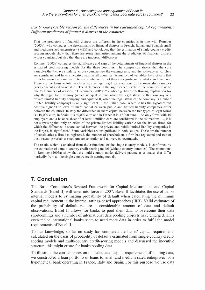
22

Box 6: One possible reason for the differences in the calculated capital requirements: Different predictors of financial distress in the countries

7. Conclusion The Basel Committee’s Revised Framework for Capital Measurement and Capital Standards (Basel II) will enter into force in 2007. Basel II facilitates the use of banks internal models to estimating probability of default when calculating the minimum capital requirement in the internal ratings-based approaches (IRB). Valid estimates of the probability of default require a considerable amount of data and default observations. Basel II allows for banks to pool their data to overcome their data shortcomings and a number of international data pooling projects have emerged. Thus even major international banks seem to need more data in order to fulfil the model requirements of Basel II.

To our knowledge, so far no study has compared the banks' capital requirements calculated on the basis of probability of defaults estimated from single-country credit-scoring models and multi-country credit-scoring models and discussed the incentive structure this might create for banks pooling data.

To illustrate the consequences on the calculated capital requirements of pooling data, we constructed a loan portfolio of loans to small and medium-sized enterprises for a hypothetical bank operating in France, Italy and Spain. For this purpose we use data

That the predictors of financial distress are different in the countries is in line with Rommer(2005a), who compares the determinants of financial distress in French, Italian and Spanish smalland medium-sized enterprises (SMEs) and concludes, that the estimation of single-country credit-scoring models show that there are some similarities among the predictors of financial distressacross countries, but also that there are important differences.

Rommer (2005a) compares the significance and sign of the determinants of financial distress in theestimated credit-scoring models for the three countries. The comparison shows that the corevariables that behave similarly across countries are the earnings ratio and the solvency ratio. Theyare significant and have a negative sign in all countries. A number of variables have effects thatdiffer between the countries in terms of whether or not they are significant or what sign they have.These are the loans to total assets ratio, size, age, legal form and one of the ownership variables(very concentrated ownership). The differences in the significance levels in the countries may bedue to a number of reasons, c.f. Rommer (2005a:26), who e.g. has the following explanation forwhy the legal form dummy (which is equal to one, when the legal status of the company is aprivate limited liability company and equal to 0, when the legal status of the company is a publiclimited liability company) is only significant in the Italian case, where it has the hypothesizedpositive sign: "The level of share capital between public and limited liability companies differbetween the countries. In Italy the difference in share capital between the two types of legal formsis 110,000 euro, in Spain it is 60,000 euro and in France it is 37,000 euro… As only firms with 10employees and a balance sheet of at least 2 million euro are considered in the estimations …, it isnot surprising that only an effect of the private limited liability variable for the Italian firms, forwhich the difference in share capital between the private and public limited liability companies isthe largest, is significant." Some variables are insignificant in both set-ups. These are the numberof subsidiaries a firm has registered, the number of shareholders a firm has registered and two ofthe ownership variables (medium concentration and not very concentrated).

The result, which is obtained from the estimations of the single-country models, is confirmed bythe estimation of a multi-country credit-scoring model (without country dummies). The estimationsin Rommer (2005a) show that the multi-country model delivers parameter estimates that differmarkedly from all the single-country credit-scoring models.


23

extracted from the Amadeus database provided by Bureau van Dijk. Using this data, the probability of default was estimated on the basis of single-country credit-scoring models and on the basis of multi-country credit-scoring models with pooled data from the three countries (with and without country dummies). The estimated probabilities of defaults are then used for calculating the minimum capital requirements for the hypothetical loan portfolio in the case of using country credit-scoring models, in the case of using a multi-country credit-scoring model with country dummies and in the case of using a multi-country credit-scoring model without country dummies.

Though our default definition is the same for the three countries and we controlled for variables such as age, size, legal form and sector, we find quite large differences in terms of the resulting minimum capital requirements for the portfolio in each of the three countries, when the probability of default is estimated using a single-country credit-scoring model compared to using multi-country credit-scoring models with and without country dummies.

One reason why the calculated capital requirements are different in the countries depending on whether the single-country or a multi-country model (with or without country dummies) is estimated could be that the predictors of financial distress differ across countries.

The results suggest that there might be incentives for cherry-picking, i.e. that banks choose a certain method because it delivers a lower capital requirement without considering what level of capital is actually appropriate to cover the overall credit risk. The overall calculated capital requirements vary with up to 18 percent depending on the choice of method for the hypothetical bank. Calculated for the individual countries it varies up to 47 percent.

Our hypothetical bank would obtain the lowest capital requirement from estimating a multi-country model with country dummies. In the situation where a bank considers pooling data with banks from other countries, the bank would also have an incentive to choose the method, which delivers the lowest capital requirement. The credit-scoring model, which delivers the lowest capital requirement, differs between the countries. For instance a bank with exposures to Italian firms would choose the single-country model, whereas a bank with the exposures to Spanish firms would choose the multi-country model with country dummies etc.

The calculations in this paper are based purely on the quantitative and technical requirements of Basel II and the EU directive proposal. We do not take into consideration effects of applying human judgment and a conservative perspective on PD estimation. The example of our hypothetical bank serves to illustrate the purely technical consequences of pooling data and the incentives it might give for banks when calculating minimum capital requirements.

The results are of particular interest for banks operating in different countries, which plan to pool data from their exposures in the various countries in order to estimate PDs like our hypothetical bank, maybe due to lack of a sufficient single-country database. The results are equally interesting for banks planning to pool data with banks from other countries to estimate PDs to make up for an insufficient database.

The overall conclusion from the analysis is that banks and supervisory authorities must be aware that the pooling of data from several countries should be done with caution. As there are not many official guidelines from authorities on the issue, we believe that the illustration in this paper of the consequences of pooling data from


24

several countries serves as an important input to the debate on how to set up credit-scoring models in banks that have cross-border exposures as well as for banks who choose to pool their data with banks in other countries. We have shown that it is not enough for banks to apply similar definitions of default and similar accounting regimes in the countries. Banks and regulators should also have a careful look into the models.


25

Literature Altman, E. I., 1968. Financial Ratios, Discriminant Analysis and the Prediction of Corporate Bankruptcy. Journal of Finance, vol. 23, no. 4, pp. 589-609 Altman, E. I. and A. Saunders, 1998. Credit risk measurement: Developments over the last 20 years. Journal of Banking and Finance, vol. 21, pp. 1721-1742 Altman, E. I., G. Marco and F. Varetto, 1994. Corporate distress diagnosis: Comparisons using linear discriminant analysis and neural networks (the Italian experience). Journal of Banking and Finance, vol. 18, pp. 505-529 Andersen, B. N., 2004. Annual Meeting of the Danish Bankers' Association on 1 December 2004. Speech by Governor Bodil Nyboe Andersen, Danmarks Nationalbank Back, B., Laitinen, T., Sere, K. and M. v. Wezel, 1996. Choosing Bankruptcy Predictors Using Discriminant Analysis, Logit Analysis, and Genetic Algorithms. Turke Centre for Computer Science, Technical Report No. 40 Balcaen, S. and H. Ooghe, 2004. Alternative methodologies in studies on business failure: do they produce better results than the classical statistical methods? Working Paper 2004/249, Faculteit Economie en Bedrijfskunde BCBS, Basel Committee on Banking Supervision, 1988. International Convergence of Capital Measurement and Capital Standards. Bank for International Settlements, July 1988 BCBS, Basel Committee on Banking Supervision, 2003. Press releas: Significant Progress on Major Issues . Bank for International Settlements, 11 October 2004 BCBS, Basel Committee on Banking Supervision, 2004. International Convergence of Capital Measurement and Capital Standards. A Revised Framework. Bank for International Settlements, June 2004 BCBS, Basel Committee on Banking Supervision, 2005. Studies on the Validation of Internal Rating Systems. Working paper no. 14, Basel Committee on Banking Supervision, February 2005 Beaver, W., 1966. Financial Ratios as Predictors of Bankruptcy. Journal of Accounting Research, vol. 6, pp. 71-102 Begley, J., Ming, J. and S. Watts, 1996. Bankruptcy Classification Errors in the 1980s: An Empirical Analysis of Altman’s and Ohlson’s Models. Review of Accounting Studies, vol. 1, pp. 267-284 Berger, A.N., Herring, R.J. and Szegö, G.P., 1995. The role of capital in financial institutions. Journal of Banking and Finance, vol. 19, pp. 393-430


26

BIS, 2004. BIS holds Annual General Meeting and releases its 74th Annual Report. Press release, June 2004 Caruana, J., 2004a. Risk management trends and the supervisory structure. Speech at the 31st General Assembly of the Geneva Association, Madrid, May 2004 Caruana, J. 2004b. Basel II – emerging market perspectives. Speech at Banker's Conference 2004, New Delhi, November 2004 Cass, D. (editor), 2002. Data hurdles. Risk magazine, vol. 15, no. 11 Dimitras, A. I., Zanakis, S. H. and C. Zopounidis, 1996. A survey of business failures with an emphasis on prediction methods and industrial applications. European Journal of Operational Research, vol. 90, pp. 487-513 Dunbar, N., 2005. Banks leapfrog the rating agencies. Risk magazine, vol. 18, no. 2 Dyrberg, A., 2004. Firms in Financial Distress: An Exploratory Analysis. WP no. 17, Danmarks Nationalbank European Commission, 2004. Proposals for directives of the European Parliament and of the Council, Re-casting Directive 2000/12/EC of the European Parliament and of the Council of 20 March 2000 relating to the taking up and pursuit of the business of credit institutions. COM (2004), 486 final. Fabi, F., Laviola, S. and P. M. Reedtz, 2004. The treatment of SME loans in the new Basel Capital Accord: Some Evaluations. Unpublished manuscript Frydman, H., Altman, E. I. and D. Kao, 1985. Introducing Recursive Partitioning for Financial Classification: The Case of Financial Distress. The Journal of Finance, vol. XL, no. 1, pp. 269-291 UK FSA, Financial Services Authority, 2005. Strengthening capital standards Greene, W., 2003. Econometric Analysis. New Jersey, USA: Prentice Hall Greuning, H. van and Bratanovic, S.B., 2003. Analyzing and Managing Banking Risk. A Framework for Assessing Corporate Governance and Financial Risk. The World Bank, Second edition, 2003. Hamerle, A., Rauhmeier, R. and D. Rösch, 2003. Uses and Misuses of Measures for Credit Rating Accuracy. Unpublished manuscript Hayden, E., 2003. Are Credit Scoring Models Sensitive With Respect to Default Definitions? Evidence from the Austrian Market. Unpublished manuscript Jenkins, S., 2003. Survival Analysis. Unpublished manuscript Jones, F. L., 1987. Current Techniques in Bankruptcy Prediction. Journal of Accounting Literature, vol. 6, pp. 131-164


27

Keefe, D., 2004. Caruana expects slower Basel II adoption. Global Risk Regulator, November 2004 Kjeldsen, K., 2004. The Role of Capital in Banks. Monetary Review, Danmarks Nationalbank, 3rd Quarter. Lando, D., 2004. Credit Risk Modeling. Theory and Applications. Princeton Series in Finance La Porta, R., F. Lopez-De-Silanes, A. Shleifer and R. Vishny, 1998. Law and Finance. The Journal of Political Economy, vol. 106, no. 6, pp. 1113-1155 Masschlein, N., 2003. The Basel II Capital Accord, SME Loans and Implications for Belgium. Financial Stability Review, Nationalbank of Belgium, June Mercer Oliver Wyman, 2005. Presentation at the Seminar on Capital Allocation in Banks. Joint training programme of Deutsche Bundesbank and Oesterreichische Nationalbank, Vienna, 27 to 28 April 2005. Moody’s Investors Service, 2001. Moody’s RiskCalc For Private Companies: Spain. Rating Methodology, July 2001 Oestereichische Nationalbank, 2004. Guidelines on Credit Risk Management, Rating Models and Validation Ohlson, J. A., 1980. Financial Ratios and the Probabilistic Prediction of Bankruptcy. Journal of Accounting Research, vol. 19, pp. 109-131 Rommer, A. D., 2005a. A Comparative Analysis of the Determinants of Financial Distress in French, Italian and Spanish firms. WP no. 26, Danmarks Nationalbank Rommer, A. D., 2005b. Testing the Assumptions of Credit-scoring Models. WP no. 28, Danmarks Nationalbank Rommer, A., D., 2005c. Firms in Financial Distress: An Exploratory Analysis. Unpublished manuscript Saurina, J. and C. Trucharte, 2003. The impact of Basel II on lending to small-and medium-sized firms. A regulatory policy assessment based on the Spanish Credit Register. Bank of Spain, June Shumway, T., 2001. Forecasting Bankruptcy More Accurately: A Simple Hazard Model. Journal of Business, vol. 74, no. 1, pp. 101-124 Thoraval, P. and Duchateau, A., 2003. Financial Stability and the New Basel Accord. Banque de France, Financial Stability Review, no. 3, November 2003.


28

Appendix 1: Calculation of the minimum capital requirement for SMEs 14 This appendix presents the formulas for calculation of the Basel II minimum capital requirement for SMEs.15 The formula specified by the Basel Committee for calculating the minimum capital requirement for a credit exposure (K*) is 8 % of the risk weight (RW) multiplied by the exposure at default (EAD):

EADRWK ××= 08.0*

For exposures not in default, the formula under the IRB-approaches for calculating the risk weight (RW) is:

( ) ( ) ( ) ( )( ) λ×××−

×−+×⎥⎥⎦

⎤

⎢⎢⎣

⎡×−⎟

⎟⎠

⎞⎜⎜⎝

⎛

−×+×=

−−

5.125.11

5.211

999.011

bbMPDLGD

RNRPDNNLGDRW

PD is the probability of default, LGD is the loss given default, and R is the assumed asset value correlation to systematic risk. N(x) denotes the cumulative distribution function for a standard normal random variable. The confidence level N-1(0.999) is set to 99.9 per cent. The first part in the squared brackets of the RW-formula is the assumed risk distribution of the losses, which is expressed as a function of LGD, PD and R.

The second part in the squared brackets ensures that the expected losses (-LGDxPD) are removed from the RW, as the minimum capital requirement under the IRB-approaches shall only cover unexpected losses. The constant 12.5 is the inverse of the capital requirement of 8 per cent. λ is a scale factor which was introduced by the Basel Committee to reiterate the Basel Committees objective of maintaining the current level of minimum capital requirements16. The Basel Committee has made it clear, that Basel II aims at the same global capital level as the 1988 Accord. The current best estimate of the scale factor from the Basel Committee is 1.06, c.f. BCBS (2004:14). The final determination of the scaling factor will probably be taken after the 5th quantitative impact study in 2005 and before the implementation of the Basel II, i.e. year-end 2006.

14 The appearance of the formulas can seem a bit arbitrary, but one must bear in mind that the formulas are a

result of economic and mathematical theory, several impact studies and not the least a pragmatic compromise between very different views and interests. The Basel Committee has chosen to be very brief in their explanation of the formulas. We will therefore not go into great detail explaining the formulas, also because the main focus in this paper is to illustrate the consequences of pooling data for corporate default risk by means of the Basel II capital requirement.

15 The notation in the EU directive proposal (see European Commission (2004)) is slightly different from the notation in the Basel Committee's Revised Framework for Capital Measurement and Capital Standards ( BCBS (2004)). We have chosen to follow the notation in the EU directive proposal.

16 For further details of the reasoning for the introduction of the scale factor see the press release, c.f. BCBS (2003: 11 October 2003).


29

The last part of the formula is dealing with maturity effects. If the effective maturity (M) measured in years is equal to 2.5, the term in the squared brackets is reduced to a function of b:

( )( )2ln05478.011852.0 PDb ×−=

The purpose of b is to transform the one-year time horizon, which is the time horizon for PD, to a "longer maturity" minimum capital requirement. The correlation to systematic risk R is determined by:

( ) SMEPDPD

ee

eeR ω−

−−−×+

−−×= −

×−

−

×−

50

50

50

50

11124.0

1112.0

The R-function is an estimate of the link (correlation) between the joint default of two separate borrowers. The IRB model relies on a single-factor asset value model to describe the co-movement of defaults in a portfolio. The single-factor can be interpreted as a variable, which represents the state of the economic cycle. IRB correlations to the single-factor are a decreasing function of the borrower's credit quality PD. The best credit quality borrowers (with a small PD) have a correlation of 24 %, and the lowest credit quality borrowers (with a high PD) have a correlation of 12 %, c.f. the R-formula.

For exposures to SME borrowers R is also a function of the firm size ωSME:

⎟⎠⎞

⎜⎝⎛ −−×=

455104.0 SSMEω

S is expressed as total annual sales in millions of euros for the companies, which have total annual sales between 5 and 50 million euro. Companies, which have reported sales under 5 million euro, will be treated as if they had sales of 5 million euro. The capital reduction increases linearly from 0 to 20 per cent with sales going from 50 to 5 million euros, and remains at 20 per cent for firms with sales figures lower than the latter threshold.

The Basel Committee has decided that the PD for corporate exposures (including SMEs) has to be larger than or equal to 0.03 %. This means that if the estimated PDs are less than 0.03 %, it should be set to 0.03 %, when calculating the risk weight. Under the foundation IRB approach, the Basel Committee has set the effective maturity (M) to 2.5 years and LGD for corporate claims to 45%

As illustrated in chart A1 the risk weight for exposures to SMEs are lower than for the exposures to corporates, and the difference increases with the size of PD.


30

Chart A1: IRB-curves for corporate and SME exposures

Note: LGD=45 %, M=2.5 and S= 25 million euro.

Risk Weight, %

0

20

40

60

80

100

120

140

160

180

0,0 1,0 2,0 3,0 4,0 5,0Probability of default, %

Corporates SMEs


31

Appendix 2: Results Table A.2.a: Results based on the PDs from the single-country credit-scoring models Number of active

companies in 2002 in the data set

The average probability of default for the companies that were active in 2002

The average capital requirement for the companies that were active in 2002, in 1000 euro

IT 35818 0.00138 2644 ES 29447 0.00135 4163 FR 41251 0.00544 2425 Note: The probability of default for each company is calculated as the average probability of default for the period 2000 – 2002. For a specific company the average probability of default can be calculated as the average of 1, 2 or 3 data points, depending on when the firm entered the sample. Table A.2.b: Results based on the PDs from the multi-country credit-scoring model (without country dummies) Number of active




IT 35818 0.00282 3899 ES 29447 0.00257 5051 FR 41251 0.00328 1985 Note: The probability of default for each company is calculated as the average probability of default for the period 2000 – 2002. For a specific company the average probability of default can be calculated as the average of 1, 2 or 3 data points, depending on when the firm entered the sample. Table A.2.c: Results based on the PDs from the multi-country credit-scoring model (with country dummies) Number of active




IT 35818 0.00154 2773 ES 29447 0.00144 3730 FR 41251 0.00520 2533 Note: The probability of default for each company is calculated as the average probability of default for the period 2000 – 2002. For a specific company the average probability of default can be calculated as the average of 1, 2 or 3 data points, depending on when the firm entered the sample.


32

Table A.2.d: The exposure of default (EAD) in the countries Number of active


The average exposure at default in the companies that were active in 2002, in 1000 euro

IT 35818 1140 ES 29447 1611 FR 41251 556


accounting-based credit-scoring models: econometric investigations

Documents