measurement of the flux of 8b solar neutrinos at the
TRANSCRIPT

Measurement of the Flux of 8B Solar Neutrinos at the
Sudbury Neutrino Observatory
James Chilton LoachLincoln College, University of Oxford
Thesis submitted in partial fulfilment of the requirements for the degree
of Doctor of Philosophy at the University of Oxford
Trinity Term, 2008

Measurement of the Flux of 8B Solar Neutrinos at the
Sudbury Neutrino Observatory
James Chilton Loach
Lincoln College, University of Oxford
Thesis submitted in partial fulfilment of the requirements for the
degree of Doctor of Philosophy at the University of Oxford
Trinity Term 2008
Abstract
The Sudbury Neutrino Observatory (SNO) was a heavy water Cerenkov detectorthat had the unique ability to measure both the total active flux of solar neutrino, usinga neutral current (NC) interaction, and the flux of electron neutrinos, using a chargedcurrent (CC) interaction. The experiment has demonstrated that neutrinos change flavourand that the total neutrino flux is consistent with the prediction of solar models.
This thesis presents results from the third phase of the experiment in which an arrayof 3He proportional counters, called Neutral Current Detectors (NCDs), were deployedin the heavy water to detect neutrons produced in NC interactions of neutrinos withdeuterium.
Converting the number of neutrons detected by the NCDs into a number of NCinteractions required a knowledge of the neutron detection efficiency. This was determinedusing two methods: with a neutron calibration source mixed into the heavy water andwith a calibrated Monte Carlo simulation. Methods for determining the strength of themixed source, using a Ge detector and the PMT array, are presented, as well as significantimprovements to the modelling of neutron propagation in the detector. Both methodswere shown to be in agreement and the neutron detection efficiency was found to be0.211 ± 0.07.
The total flux of solar neutrinos and the flux of electron neutrinos were statisticallyextracted from the NCD phase data using a technique that allowed a subset of the sys-tematic parameters to have their values constrained by the neutrino data. The measuredflux was
ΦNC = 5.443+0.329−0.327 (stat.) +0.318
−0.301 (syst.) × 106 ν cm−2 s−1
which is good agreement with standard solar models. The ratio of CC to NC fluxes, whichis the fraction of electron neutrinos in the active neutrino flux, was found to be
ΦCC
ΦNC= 0.318+0.030
−0.031 (total)
On the assumption that the reduced flux of electron neutrinos was due to neutrino oscil-lations and that CPT invariance holds, a global fit to the results of solar experiments andthe reactor anti-neutrino experiment KamLAND yielded the neutrino mixing parameters
∆m2 = 7.94+0.42−0.26 × 10⁻⁵ eV2 θ = 33.8+1.4
−1.3 degrees

For my parents.
i

Acknowledgements
There are many people to thank for making this work possible and my years as a graduate
student the formative ones that they’ve turned out to be.
Above all I want to thank my supervisor Nick Jelley, who has been a source of
optimism, guidance, and patience throughout.
I’ve shared the ups and downs of graduate life with the Oxford students Jeanne, Jess,
Charlotte, Wan, Gaby and Helen. The journey would not have been the same without
sightseeing in Squamish, swimming in Sudbury or the relentless good humour from the
far corner of the office.
I’ve enjoyed working with others at Oxford, notably Simon, Dave, Steve and, not
least, Nick West, who helped both me and SNOMAN survive my forays into the code.
Beverly, Kim and Sue have been patient guides through the mysteries of university regu-
lations.
Within SNO I’ve had the pleasure of working with, and learning from, a remarkable
group of people. Of the many I could mention, I want to thank a few in particular: Gene,
Jimmy, Melin, Bruce and Carsten, who were fellow-neutron analysts, and Nikolai, Scott,
Jason Goon and Blair of the signal extraction group. Jason Detwiler, Keith, Jaret, John
Roberts, Marc and others have answered my questions. Christine, Aksel, Hamish and Art
have given their time, energy and thoughts whenever I have asked.
I owe a huge amount of gratitude - I cannot express how much - to the Berkeley
group who have supported me over the last year. In particular to Alan, for your sound
advice and support behind the scenes, and to Gersende for sharing your goodwill and tiny
office. It has been a privilege to work with such a pleasant and intelligent group of people
and to spend time in such a beautiful corner of the world.
My final thanks are for Elisa who encouraged me to start this work all those years
ago, and for Carolyn and Marta, whose endless patience and support helped me reach the
end.
ii

Was the Sun designed to provide a convenient
laboratory for studying neutrino masses via oscillation?
It almost seems that way.
JOHN BAHCALL
Neutrino Astrophysics (1989)
i

Contents
1 Neutrinos and the Sun 1
1.1 How the Sun shines . . . . . . . . . . . . . . . . . . . . . . . . . . . . . . . 3
1.1.1 The source of the Sun’s energy . . . . . . . . . . . . . . . . . . . . 3
1.1.2 Modelling the Sun . . . . . . . . . . . . . . . . . . . . . . . . . . . 6
1.2 The physics of massive neutrinos . . . . . . . . . . . . . . . . . . . . . . . 13
1.2.1 Neutrinos and the standard model . . . . . . . . . . . . . . . . . . . 13
1.2.2 Mixing . . . . . . . . . . . . . . . . . . . . . . . . . . . . . . . . . . 14
1.2.3 Matter enhancement . . . . . . . . . . . . . . . . . . . . . . . . . . 16
1.3 Evidence for neutrino mass and oscillations . . . . . . . . . . . . . . . . . . 18
1.3.1 Oscillation parameters . . . . . . . . . . . . . . . . . . . . . . . . . 18
1.3.2 The solar sector . . . . . . . . . . . . . . . . . . . . . . . . . . . . . 19
1.3.3 The atmospheric sector . . . . . . . . . . . . . . . . . . . . . . . . . 21
1.3.4 θ13 and CP violation . . . . . . . . . . . . . . . . . . . . . . . . . . 22
1.3.5 Remaining questions . . . . . . . . . . . . . . . . . . . . . . . . . . 22
2 Measuring the flux of solar neutrinos 24
2.1 The three phases of SNO . . . . . . . . . . . . . . . . . . . . . . . . . . . . 24
2.1.1 The D2O phase . . . . . . . . . . . . . . . . . . . . . . . . . . . . . 28
2.1.2 The Salt phase . . . . . . . . . . . . . . . . . . . . . . . . . . . . . 28
2.1.3 The NCD phase . . . . . . . . . . . . . . . . . . . . . . . . . . . . . 29
2.2 Detecting neutrons . . . . . . . . . . . . . . . . . . . . . . . . . . . . . . . 31
2.2.1 The NCD array . . . . . . . . . . . . . . . . . . . . . . . . . . . . . 31
2.2.2 Data acquisition . . . . . . . . . . . . . . . . . . . . . . . . . . . . . 35
2.2.3 Events in the counters . . . . . . . . . . . . . . . . . . . . . . . . . 36
2.3 Detecting Cerenkov light . . . . . . . . . . . . . . . . . . . . . . . . . . . . 39
2.3.1 The PMT array . . . . . . . . . . . . . . . . . . . . . . . . . . . . . 39
2.4 Calibration . . . . . . . . . . . . . . . . . . . . . . . . . . . . . . . . . . . 40
2.4.1 Electronics calibrations . . . . . . . . . . . . . . . . . . . . . . . . . 40
2.4.2 Physics calibrations . . . . . . . . . . . . . . . . . . . . . . . . . . . 40
ii

2.5 Thesis outline . . . . . . . . . . . . . . . . . . . . . . . . . . . . . . . . . . 42
3 The neutron detection efficiency 44
3.1 Neutrons in SNO . . . . . . . . . . . . . . . . . . . . . . . . . . . . . . . . 44
3.2 Goals and methods . . . . . . . . . . . . . . . . . . . . . . . . . . . . . . . 46
3.3 The 24Na method . . . . . . . . . . . . . . . . . . . . . . . . . . . . . . . . 48
3.3.1 Overview . . . . . . . . . . . . . . . . . . . . . . . . . . . . . . . . 48
3.3.2 Measurements . . . . . . . . . . . . . . . . . . . . . . . . . . . . . . 49
3.3.3 Efficiency . . . . . . . . . . . . . . . . . . . . . . . . . . . . . . . . 50
3.3.4 Results . . . . . . . . . . . . . . . . . . . . . . . . . . . . . . . . . . 56
3.4 The point source method . . . . . . . . . . . . . . . . . . . . . . . . . . . . 57
3.4.1 Overview . . . . . . . . . . . . . . . . . . . . . . . . . . . . . . . . 57
3.4.2 Results . . . . . . . . . . . . . . . . . . . . . . . . . . . . . . . . . . 58
4 Modelling neutron propagation 59
4.1 The SNOMAN Monte Carlo . . . . . . . . . . . . . . . . . . . . . . . . . . 60
4.2 Nuclear reactions and media . . . . . . . . . . . . . . . . . . . . . . . . . . 61
4.2.1 Nuclear reactions . . . . . . . . . . . . . . . . . . . . . . . . . . . . 61
4.2.2 Media . . . . . . . . . . . . . . . . . . . . . . . . . . . . . . . . . . 63
4.3 Detector geometry . . . . . . . . . . . . . . . . . . . . . . . . . . . . . . . 65
4.3.1 Overview . . . . . . . . . . . . . . . . . . . . . . . . . . . . . . . . 65
4.3.2 The NCD array . . . . . . . . . . . . . . . . . . . . . . . . . . . . . 65
4.3.3 The acrylic vessel . . . . . . . . . . . . . . . . . . . . . . . . . . . . 71
4.3.4 Neutron calibration sources . . . . . . . . . . . . . . . . . . . . . . 73
4.4 Calibration sources . . . . . . . . . . . . . . . . . . . . . . . . . . . . . . . 74
4.4.1 Overview . . . . . . . . . . . . . . . . . . . . . . . . . . . . . . . . 74
4.4.2 The 252Cf source . . . . . . . . . . . . . . . . . . . . . . . . . . . . 74
4.4.3 The AmBe sources . . . . . . . . . . . . . . . . . . . . . . . . . . . 78
5 Source strength measurements using a Ge detector 81
5.1 Ge detectors in general, and the SNO Ge detector in particular . . . . . . . 82
5.1.1 Ge detectors . . . . . . . . . . . . . . . . . . . . . . . . . . . . . . . 82
5.1.2 Energy deposition spectra . . . . . . . . . . . . . . . . . . . . . . . 84
5.1.3 The SNO Ge detector . . . . . . . . . . . . . . . . . . . . . . . . . 86
5.1.4 Calibration sources . . . . . . . . . . . . . . . . . . . . . . . . . . . 88
5.2 A Monte Carlo simulation in SNOMAN . . . . . . . . . . . . . . . . . . . . 90
5.2.1 Verification . . . . . . . . . . . . . . . . . . . . . . . . . . . . . . . 94
5.3 Full-energy peak integration . . . . . . . . . . . . . . . . . . . . . . . . . . 95
iii

5.3.1 Determining peak areas . . . . . . . . . . . . . . . . . . . . . . . . 95
5.3.2 Comparison between the methods . . . . . . . . . . . . . . . . . . . 98
5.4 Tuning the dead layer and the KCl anomaly . . . . . . . . . . . . . . . . . 98
5.4.1 Analysis of calibration data . . . . . . . . . . . . . . . . . . . . . . 98
5.4.2 Tuning the dead layer . . . . . . . . . . . . . . . . . . . . . . . . . 102
5.4.3 The stability of the detector . . . . . . . . . . . . . . . . . . . . . . 103
5.4.4 Self absorption in the calibration sources . . . . . . . . . . . . . . . 106
5.4.5 Source strengths . . . . . . . . . . . . . . . . . . . . . . . . . . . . 108
5.4.6 The efficiency for detecting 24Na gammas . . . . . . . . . . . . . . . 109
5.5 Dead time . . . . . . . . . . . . . . . . . . . . . . . . . . . . . . . . . . . . 109
5.5.1 Understanding and modelling detector dead time . . . . . . . . . . 109
5.5.2 Dead time in the 24Na data . . . . . . . . . . . . . . . . . . . . . . 110
5.5.3 Dead time in the mixed source data . . . . . . . . . . . . . . . . . . 111
5.6 The 24Na source strength . . . . . . . . . . . . . . . . . . . . . . . . . . . . 113
5.6.1 Probability of photodisintegration . . . . . . . . . . . . . . . . . . . 113
5.6.2 Source strengths . . . . . . . . . . . . . . . . . . . . . . . . . . . . 116
5.7 The 222Rn source strengths . . . . . . . . . . . . . . . . . . . . . . . . . . . 117
5.7.1 Introduction . . . . . . . . . . . . . . . . . . . . . . . . . . . . . . . 117
5.7.2 The efficiency for detecting 214Bi gammas . . . . . . . . . . . . . . 119
5.7.3 Peak areas and dead time . . . . . . . . . . . . . . . . . . . . . . . 124
5.7.4 Source strengths . . . . . . . . . . . . . . . . . . . . . . . . . . . . 126
6 Source strength measurements using the PMT array 128
6.1 The 252Cf source strength . . . . . . . . . . . . . . . . . . . . . . . . . . . 128
6.1.1 Measurements . . . . . . . . . . . . . . . . . . . . . . . . . . . . . . 128
6.2 The 24Na source strengths . . . . . . . . . . . . . . . . . . . . . . . . . . . 132
6.2.1 Overview . . . . . . . . . . . . . . . . . . . . . . . . . . . . . . . . 132
6.2.2 Data selection . . . . . . . . . . . . . . . . . . . . . . . . . . . . . . 135
6.2.3 Radial neutron production profile (fC) . . . . . . . . . . . . . . . . 136
6.2.4 Probability of photodisintegration (fP ) . . . . . . . . . . . . . . . . 141
6.2.5 Source strengths . . . . . . . . . . . . . . . . . . . . . . . . . . . . 145
6.3 The AmBe source strengths . . . . . . . . . . . . . . . . . . . . . . . . . . 149
6.3.1 Overview . . . . . . . . . . . . . . . . . . . . . . . . . . . . . . . . 149
6.3.2 Source strengths . . . . . . . . . . . . . . . . . . . . . . . . . . . . 150
6.4 Summary . . . . . . . . . . . . . . . . . . . . . . . . . . . . . . . . . . . . 152
iv

7 The Neutron Detection Efficiency Using Point Sources 153
7.1 Point source data . . . . . . . . . . . . . . . . . . . . . . . . . . . . . . . . 154
7.1.1 Overview . . . . . . . . . . . . . . . . . . . . . . . . . . . . . . . . 154
7.1.2 The point source data . . . . . . . . . . . . . . . . . . . . . . . . . 155
7.1.3 Run selection . . . . . . . . . . . . . . . . . . . . . . . . . . . . . . 156
7.1.4 Source positions . . . . . . . . . . . . . . . . . . . . . . . . . . . . . 157
7.1.5 Detection efficiencies . . . . . . . . . . . . . . . . . . . . . . . . . . 161
7.1.6 Simulations . . . . . . . . . . . . . . . . . . . . . . . . . . . . . . . 161
7.2 The hydrogen fraction . . . . . . . . . . . . . . . . . . . . . . . . . . . . . 162
7.2.1 Method . . . . . . . . . . . . . . . . . . . . . . . . . . . . . . . . . 162
7.2.2 Results . . . . . . . . . . . . . . . . . . . . . . . . . . . . . . . . . . 164
7.3 The quality of the Monte Carlo . . . . . . . . . . . . . . . . . . . . . . . . 166
7.4 The NC neutron detection efficiency . . . . . . . . . . . . . . . . . . . . . . 169
7.4.1 Result . . . . . . . . . . . . . . . . . . . . . . . . . . . . . . . . . . 169
7.4.2 Systematic uncertainties . . . . . . . . . . . . . . . . . . . . . . . . 170
7.5 Other neutron detection efficiencies . . . . . . . . . . . . . . . . . . . . . . 174
7.6 Summary . . . . . . . . . . . . . . . . . . . . . . . . . . . . . . . . . . . . 174
8 Measuring the NC flux 176
8.1 Fitting using maximum likelihood . . . . . . . . . . . . . . . . . . . . . . . 177
8.1.1 Overview . . . . . . . . . . . . . . . . . . . . . . . . . . . . . . . . 177
8.1.2 The NCD phase formalism . . . . . . . . . . . . . . . . . . . . . . . 177
8.2 Probability distribution functions . . . . . . . . . . . . . . . . . . . . . . . 180
8.2.1 Signals and backgrounds . . . . . . . . . . . . . . . . . . . . . . . . 180
8.2.2 Observables in the PMT array . . . . . . . . . . . . . . . . . . . . . 182
8.2.3 Observables in the NCD array . . . . . . . . . . . . . . . . . . . . . 185
8.2.4 Instrumental and high level cuts . . . . . . . . . . . . . . . . . . . . 186
8.3 Fluxes and events . . . . . . . . . . . . . . . . . . . . . . . . . . . . . . . . 188
8.4 Systematic uncertainties . . . . . . . . . . . . . . . . . . . . . . . . . . . . 190
8.4.1 Using the data . . . . . . . . . . . . . . . . . . . . . . . . . . . . . 190
8.4.2 PMT stream . . . . . . . . . . . . . . . . . . . . . . . . . . . . . . . 193
8.4.3 NCD stream . . . . . . . . . . . . . . . . . . . . . . . . . . . . . . . 194
8.5 The MXF code . . . . . . . . . . . . . . . . . . . . . . . . . . . . . . . . . 195
8.5.1 Three codes . . . . . . . . . . . . . . . . . . . . . . . . . . . . . . . 195
8.5.2 Bias testing . . . . . . . . . . . . . . . . . . . . . . . . . . . . . . . 197
8.5.3 Blindness . . . . . . . . . . . . . . . . . . . . . . . . . . . . . . . . 201
8.6 Results . . . . . . . . . . . . . . . . . . . . . . . . . . . . . . . . . . . . . . 201
v

9 Conclusions 206
A The decay schemes of 232Th and 238U 210
B Combining measurements 213
C The SNOMAN geometry 214
C.1 Requirements and structure of the code . . . . . . . . . . . . . . . . . . . . 214
C.2 Testing the geometry . . . . . . . . . . . . . . . . . . . . . . . . . . . . . . 215
D Time series analysis 218
E The mass attenuation coefficient 219
F The total peak area method 220
G The composition of the mixed source 223
H Neutron poison in the NCD phase 225
H.1 Introduction . . . . . . . . . . . . . . . . . . . . . . . . . . . . . . . . . . . 225
H.2 Neutron poisons . . . . . . . . . . . . . . . . . . . . . . . . . . . . . . . . . 226
H.3 Statistical subtraction . . . . . . . . . . . . . . . . . . . . . . . . . . . . . 229
H.3.1 Overview . . . . . . . . . . . . . . . . . . . . . . . . . . . . . . . . 229
H.3.2 Method . . . . . . . . . . . . . . . . . . . . . . . . . . . . . . . . . 229
H.3.3 Results . . . . . . . . . . . . . . . . . . . . . . . . . . . . . . . . . . 230
H.4 Poison phase background PDFs . . . . . . . . . . . . . . . . . . . . . . . . 233
H.4.1 Overview . . . . . . . . . . . . . . . . . . . . . . . . . . . . . . . . 233
H.4.2 Method . . . . . . . . . . . . . . . . . . . . . . . . . . . . . . . . . 233
H.4.3 Results . . . . . . . . . . . . . . . . . . . . . . . . . . . . . . . . . . 233
I Neutrino flux fit results 235
Bibliography 241
vi

List of Figures
1.1 The pp chain. . . . . . . . . . . . . . . . . . . . . . . . . . . . . . . . . . . 7
1.2 The radial production profile of pp chain neutrinos [1]. . . . . . . . . . . . 10
1.3 The predicted solar neutrino energy spectrum [2] showing pp (solid lines)
and CNO neutrinos (dashed lines). . . . . . . . . . . . . . . . . . . . . . . 11
1.4 Agreement between sound speeds calculated using standard solar models
(dashed line) and those measured helioseismologically [3]. . . . . . . . . . . 13
1.5 The MSW effect, for a small vacuum mixing angle [4]. The masses of the
νe and νµ flavour eigenstates as a function of solar radius (light lines). The
top dark line shows the development of a νe as it leaves the production
point in the solar core and converts into a νµ. . . . . . . . . . . . . . . . . 17
1.6 Contours showing allowed values of the solar sector mixing parameters [5].
This plot does not include the results from this thesis. . . . . . . . . . . . . 20
1.7 Contours showing allowed values for the atmospheric mixing parameters [6]. 21
2.1 Diagrams of the neutrino interactions in SNO. Adapted from [7]. . . . . . . 25
2.2 The SNO detector. Adapted from [8]. . . . . . . . . . . . . . . . . . . . . . 27
2.3 Results from the salt phase [9]. The plot shows the flux of muon + tau
neutrinos versus the flux of electron neutrinos. . . . . . . . . . . . . . . . . 29
2.4 The NCD array looking down into the detector in the negative z direction. 32
2.5 An NCD string. Adapted from [8]. . . . . . . . . . . . . . . . . . . . . . . 34
2.6 Schematic diagram showing the main components of the NCD electronics.
The numbers in grey indicate the dead time associated with each component. 35
2.7 Example pulses: neutron (top left), alpha (top right), J3 instrumental
(bottom left), and oscillatory noise event (bottom right). In the neutron
and alpha panels the red lines are pulses where the ionisation was deposited
along a path oriented close to the counter radius, perpendicular to the wire,
and the black lines represent pulses where it was deposited close to parallel
with the wire. . . . . . . . . . . . . . . . . . . . . . . . . . . . . . . . . . . 37
2.8 Shaper-ADC energy spectrum for the neutrino data set. . . . . . . . . . . . 37
vii

2.9 Different types of neutron event showing the amounts of energy deposited
in the gas. . . . . . . . . . . . . . . . . . . . . . . . . . . . . . . . . . . . . 38
2.10 The calibration source manipulator system. Adapted from [8]. . . . . . . . 39
3.1 D2O and salt phase neutron detection efficiencies as a function of radius.
The points are measurements taken with a 252Cf source [9]. The fits are to
analytical models of the dependence of the efficiency on radius. . . . . . . . 46
3.2 The decay scheme of 24Na. The dominant decay channel (BR ∼ 1.0) is the
one containing the 1.369 and 2.754 MeV gammas. . . . . . . . . . . . . . . 49
3.3 The NCD neutron capture rate as a function of time in the 2005 measure-
ment [10]. The green points show the neutron detection rate in each run
and the black points show it corrected to the time at the start of counting. 50
3.4 Mixing of the 24Na: the ratio of the data and Monte Carlo radial light dis-
tributions (top plots) and the ratio of the 2006 and 2005 light distributions
(lower plots). Time increases from left to right and the rightmost plots
correspond to the steady state. . . . . . . . . . . . . . . . . . . . . . . . . 56
4.1 The 2H(n,2n)1H and 16O(n,α)13C cross sections as a function of energy. . . 63
4.2 Measurements of the mass of NaCl in the heavy water. Neutrino data were
taken in the period between the dashed lines. The conductivity measure-
ments were fit to a decaying exponential. . . . . . . . . . . . . . . . . . . . 66
4.3 The Monte Carlo geometry of an NCD string showing the top of a string
(left) and the section in between two counters (right). . . . . . . . . . . . . 68
4.4 The Monte Carlo geometry of an NCD cable. . . . . . . . . . . . . . . . . . 69
4.5 Simulated field lines at the end of a counter [11]. The region to the left of
line B corresponds to one half of the lightly hatched regions in Figure 4.3. . 70
4.6 NCD phase neutron calibration sources. . . . . . . . . . . . . . . . . . . . . 72
4.7 z-profile of source neutron captures on the materials of a source. The source
activity was located at z = 0. . . . . . . . . . . . . . . . . . . . . . . . . . 73
4.8 Energy spectra of 252Cf and NC neutrons. . . . . . . . . . . . . . . . . . . 75
4.9 252Cf gamma multiplicity distributions in the Monte Carlo compared with
experiment (left) and the energy spectrum from a 252Cf salt run simulation
(right). . . . . . . . . . . . . . . . . . . . . . . . . . . . . . . . . . . . . . . 76
4.10 An experimental AmBe energy spectrum from [12] (left) and the Monte
Carlo energy spectrum (right) which is the average of two measured spectra. 79
4.11 The energy-dependence of the neutron capture cross section on hydrogen
(left) and the NCD array neutron capture efficiency as a function of neutron
energy for a source placed just outside the acrylic vessel (right). . . . . . . 80
viii

5.1 Processes by which a gamma can interact in a Ge detector. Event 1
contributes to the Compton continuum; events 2 and 3 lie in the full-
energy peak; in event 4 a pair-produced gamma escapes and all other en-
ergy is absorbed, leaving a count in the first escape peak; in event 5 two
pair-produced gammas escape, leaving a count in the second escape peak.
Adapted from [13] . . . . . . . . . . . . . . . . . . . . . . . . . . . . . . . . 85
5.2 A 24Na energy deposition spectrum produced by the SNO Ge detector. . . 86
5.3 The Ge detector and Marinelli beaker geometry, as modelled in the Monte
Carlo simulation. The actual Marinelli beakers had gently sloping sides. . . 87
5.4 Background energy spectrum collected with an empty Marinelli beaker for
4 days. The highest ADC bin corresponds to 2.826 MeV. . . . . . . . . . . 88
5.5 Decay schemes for 40K (left) and 88Y (right). Adapted from [14]. . . . . . . 91
5.6 Simulated and experimental 24Na energy deposition spectra. . . . . . . . . 94
5.7 Comparisons between relative peak heights in data and Monte Carlo. 24Na
2.754 / 1.369 (top left), 24Na sum peak / 1.369 (top right), 88Y 1.836 /
0.898 (bottom left), 88Y sum / 0.898 (bottom right). In the 24Na plots the
comparison was made for all three measurements and for 88Y it was made
for the two highest statistics mixed source runs. . . . . . . . . . . . . . . . 96
5.8 An example 24Na peak showing the peak and background regions in the
TPA interpolation method. . . . . . . . . . . . . . . . . . . . . . . . . . . . 97
5.9 An example fit peak from the mixed source data showing the step function
background continuum and eight Gaussians that describe the peak. The
data points are green and the fit is black. Figure provided by Nirel [15]. . . 97
5.10 Efficiency as a function of energy measured using the mixed calibration
source. The small χ2/d.o.f. is because the efficiencies were assumed to be
uncorrelated in this fit. . . . . . . . . . . . . . . . . . . . . . . . . . . . . . 101
5.11 Two example Monte Carlo models for dead layer fitting: 383.8 keV 133Ba
peak (left) and 834.8 keV 54Mn peak (right). . . . . . . . . . . . . . . . . . 102
5.12 Measured minus simulated efficiency as a function of energy using the best
fit dead layer. . . . . . . . . . . . . . . . . . . . . . . . . . . . . . . . . . . 104
5.13 The best fit dead layer for each calibration source. Above the dashed line
the discrepancy between the three sources is seen clearly. The agreement
between the solid and second liquid KCl source (below the line) shows
the ability of the Monte Carlo to extrapolate between two sources of very
different density. . . . . . . . . . . . . . . . . . . . . . . . . . . . . . . . . 104
5.14 Stability of measurements made with the solid KCl source. Uncertainties
are statistical only. . . . . . . . . . . . . . . . . . . . . . . . . . . . . . . . 105
ix

5.15 Stability of measurements made with the mixed source: 383 keV 133Ba
peak (left) and 1116 65Zn peak (right). Uncertainties are statistical only. . 105
5.16 Dead time fit and residuals for the 1.369 MeV peak in the 2005 24Na mea-
surement. . . . . . . . . . . . . . . . . . . . . . . . . . . . . . . . . . . . . 112
5.17 The left hand plot shows the ratio of fit to DAQ dead time fractions in
the 2005 24Na measurement (1.369 MeV peak in red and 2.754 MeV peak
in blue). The right hand plot shows the effect of the discrepancy on the
recorded number of counts. . . . . . . . . . . . . . . . . . . . . . . . . . . . 112
5.18 The radon can and Ge detector geometry as implemented in the Monte
Carlo simulation. . . . . . . . . . . . . . . . . . . . . . . . . . . . . . . . . 118
5.19 A measured radon spectrum with select gammas from 214Pb and 214Bi
labelled. . . . . . . . . . . . . . . . . . . . . . . . . . . . . . . . . . . . . . 121
5.20 A Monte Carlo radon spectrum. Simulations runs with decays of the radon
daughter 214Bi only. . . . . . . . . . . . . . . . . . . . . . . . . . . . . . . . 121
5.21 An example 1764 keV full-energy peak showing the background regions on
both sides. Data is from the H2O measurement. . . . . . . . . . . . . . . . 124
5.22 Dead time fit and residuals for the 1764 keV peak in the D2O data (top)
and for the 2204 keV peak in the H2O data (bottom). . . . . . . . . . . . . 127
6.1 The 3He proportional counter apparatus used in the direct counting mea-
surement of the 252Cf source strength. Section (left) and plan (right). . . . 130
6.2 The 200 µs array capture efficiency (top left), 1000 µs capture efficiency
(top right), 200-1000 µs correction factor (bottom left) and the correction to
the efficiency measured with an unencapsulated source to make it applicable
for the acrylic 252Cf source (bottom right). All plots show the variation of
the quantity as a function of the distance of the production point above the
bottom of the well. Points are fit to polynomials to illustrate the general
dependence - there is no physical motivation for the functional forms. The
efficiencies in the top two plots are percentages. . . . . . . . . . . . . . . . 133
6.3 Measured energy-radius distributions for 252Cf (left) and 24Na (right). The
box highlights the analysis region. These plots are intended to illustrate
the relative distributions of events in energy-radius space; there happens
to be more events in the 24Na plot but this is of no consequence. . . . . . . 137
6.4 Energy-radius distributions for three PMT backgrounds: Monte Carlo sim-
ulation of 252Cf gammas (top left), 24Na gammas (top right) and (mainly)
low energy background events from a neutrino run (bottom). The box
highlights the analysis region. . . . . . . . . . . . . . . . . . . . . . . . . . 138
x
6.5 Radial neutron production profile of 24Na photodisintegration neutrons
(left) and radial capture profiles (right) of 24Na neutrons (red) and 252Cf
neutrons (blue). The y-axis units are arbitrary. The plots show the actual
positions of the verticies in the Monte Carlo rather than ones reconstructed
using position fitters. . . . . . . . . . . . . . . . . . . . . . . . . . . . . . . 139
6.6 Correction factor fC by radial bin (left) and as a function of lower radial
cut (right). The error bars give the statistical uncertainties and the green
bands give the systematic uncertainties. . . . . . . . . . . . . . . . . . . . . 139
6.7 Delrin mass attenuation coefficient experimental configuration, as simu-
lated in SNOMAN. . . . . . . . . . . . . . . . . . . . . . . . . . . . . . . . 142
6.8 Energy distribution of 2.754 MeV gammas after a single Compton Scatter-
ing (left); D2O total and photodisintegration cross sections (right). . . . . . 144
6.9 Fits to the radioactive decay law, with the 24Na half life fixed, yielding
activities at the start of the first run in each data set. Dry run (top), 2005
(middle) and 2006 (bottom). . . . . . . . . . . . . . . . . . . . . . . . . . . 146
6.10 Raw and corrected source strengths by bin (left) and as a function of lower
radial cut (right) for the 2005 measurement (top) and 2006 measurement
(bottom). Error bars are statistical. . . . . . . . . . . . . . . . . . . . . . . 147
6.11 Source strengths as a function of run number (top) projected onto the y-
axes (bottom). Medium rate source (left) and high rate source (right).
Uncertainties are statistical only. . . . . . . . . . . . . . . . . . . . . . . . 151
6.12 Source strengths as a function of radial bin. Medium rate source (left) and
high rate source (right). Uncertainties are statistical only and the central
values have been corrected with fC . . . . . . . . . . . . . . . . . . . . . . . 152
7.1 Source positions in one of the vertical planes (red dots) in a full AmBe scan
[16]. . . . . . . . . . . . . . . . . . . . . . . . . . . . . . . . . . . . . . . . 155
7.2 Source positions selected for use in this analysis (red dots). . . . . . . . . . 157
7.3 The dependence of neutron capture efficiency on source position for posi-
tions 12 and 9, which were the extreme positions in y. Simulations were
generated using the OCA (see text) NCD array geometry. . . . . . . . . . . 159
7.4 Representative examples of the measured efficiencies of different rings as
a function of time. The data points are for central runs. The grey boxes
indicate the fit uncertainties. 6-ring efficiencies are shown on the left (N, L
and I rings) and 3-ring efficiencies on the right (N+M, L+K and J+I rings).160
xi

7.5 Example Monte Carlo models gr(fH) showing ring efficiencies as a function
of the hydrogen fraction. Simulations are for the central position and used
the OCA geometry. The 6-ring efficiency for the N strings is shown on the
left and the 3-ring efficiency for the N+M rings combined on the right. . . 163
7.6 Example hydrogen fraction fits for the central source position using the
OCA geometry. Shown are fit results (left) and residuals (right) for 6-rings
(top) and 3-rings (bottom). . . . . . . . . . . . . . . . . . . . . . . . . . . 165
7.7 3-ring fit hydrogen fractions (top) and efficiency scale (bottom) by fit num-
ber (left) and manipulator source radius (right). . . . . . . . . . . . . . . . 167
7.8 The ratio of measured to predicted efficiencies at 13 source positions. The
left section contains the data points within the array, used to tune the
hydrogen fraction. The middle section contains the points at the top and
bottom of the array. And the right section contains points outside the array.
The source positions for the left two sections are from the manipulator.
Those in the right section are fit. The yellow bar gives the correlated
uncertainty on the data due to the AmBe source strengths. . . . . . . . . . 168
7.9 Comparison of 252Cf source data (red points) and Monte Carlo (green
points) along the central, vertical axis of the detector [17]. Efficiencies
were determined using the TSA analysis (see Appendix D). The error bars
are statistical only. . . . . . . . . . . . . . . . . . . . . . . . . . . . . . . . 169
7.10 NC capture efficiencies as a function of hydrogen fraction for OCA geometry
(left) and LRF geometry (right). . . . . . . . . . . . . . . . . . . . . . . . . 170
7.11 The effect of absorption in the acrylic vessel on the NC neutron capture
efficiency. The parameter varied is the density of hydrogen in the acrylic
vessel. The left hand plot shows the NC efficiency as a function of the
change in density; the right hand plot shows the variation of captures in
various geometry regions. . . . . . . . . . . . . . . . . . . . . . . . . . . . 171
8.1 Signal PDFs. The distributions in the PMT observables for CC, ES and
NC are shown in energy (top left), cosine of reconstructed direction with
respect to that of the Sun (top right) and radius (centre left). Note that the
shapes of the energy PDFs for CC and ES events were allowed to float in
the fits. The background radial distributions are shown centre right. The
bottom plot shows the distributions in the NCD observable shaper-ADC
energy. Normalisations should be considered arbitrary. . . . . . . . . . . . 183
8.2 Results of bias tests run on the ensemble of fake data sets with properties
equivalent to the neutrino data set. . . . . . . . . . . . . . . . . . . . . . . 200
xii

8.3 Fit results obtained using the Monte Carlo alpha PDF. In the PMT en-
ergy plot two spectra are shown for both ES and CC: the ones labelled
‘E con. equiv.’ are the Monte Carlo energy spectra normalised to the to-
tal number of ES or CC events; the ones labelled ‘E uncon.’ are the fit,
energy-unconstrained, spectra. . . . . . . . . . . . . . . . . . . . . . . . . . 202
8.4 Comparison of the flux results in different phases and, for ES, also with
the results of Super Kamiokande-I [18]. The red bars are the statistical
uncertainties and the blue bars are the total uncertainties. . . . . . . . . . 204
8.5 The cos θ⊙ distribution in the three lowest energy bins. 6.0-6.5 MeV (left)
to 7.0-7.5 MeV (right). . . . . . . . . . . . . . . . . . . . . . . . . . . . . . 204
8.6 Neutrino oscillation contours from a combined fit to the three phases of
SNO data (top), global fit to all solar data (bottom right) and global fit to
all solar data and KamLAND. . . . . . . . . . . . . . . . . . . . . . . . . . 205
A.1 The 232Th decay chain. The Q-values are quoted in MeV and the gamma
energies in keV. Adapted from [19]. . . . . . . . . . . . . . . . . . . . . . . 211
A.2 The 238U decay chain. The Q-values are quoted in MeV and the gamma
energies in keV. Adapted from [19]. . . . . . . . . . . . . . . . . . . . . . . 212
C.1 The canned 24Na source and manipulator, as modelled in SNOMAN. The
dots are the intersections of simulated neutrino events with the boundaries
of geometry regions. . . . . . . . . . . . . . . . . . . . . . . . . . . . . . . 217
F.1 Schematic diagram illustrating the TPA method. . . . . . . . . . . . . . . 221
H.1 Schematic diagram showing the effect of adding poison on the signal counts
S and background counts B in a region of pulse parameter space. ε is the
ratio of neutrino and poison livetimes and χ is the ratio of signal detection
rates in the neutrino and poison phases (the effectiveness of the poison). . 229
H.2 Extracted number of neutrons and fractional error as a function of the ratio
of neutrino and poison livetimes. Salt phase poisoning is assumed in the
left hand plot. The vertical lines correspond to poison livetimes of 60 and
90 days. . . . . . . . . . . . . . . . . . . . . . . . . . . . . . . . . . . . . . 231
H.3 Example fit using a 60 day poison phase PDF and a background to signal
ratio of 2.115. . . . . . . . . . . . . . . . . . . . . . . . . . . . . . . . . . . 234
xiii

List of Tables
1.1 Important solar parameters (from [1]). . . . . . . . . . . . . . . . . . . . . 8
2.1 Calibration sources used during the NCD phase. . . . . . . . . . . . . . . . 41
3.1 Percentages of neutrons produced by NC neutrino interactions capturing in
various regions and on various nuclei, taken from a Monte Carlo simulation.
Missing entries are zero or negligible. The inactive NCD regions are regions
where the ionisation was not collected. . . . . . . . . . . . . . . . . . . . . 45
3.2 Measurements of the 24Na source strength An (in n s−1). The strengths
for each measurement were scaled to a common reference time, mass and
spatial distribution. . . . . . . . . . . . . . . . . . . . . . . . . . . . . . . . 51
3.3 Summary of the results of the 24Na method broken down in components
correlated and uncorrelated between the measurements. . . . . . . . . . . . 57
5.1 Mixed source radioisotopes [20, 14]. The reference time for the activities is
Feb 1st 2005 06:00:00 EDT. . . . . . . . . . . . . . . . . . . . . . . . . . . 90
5.2 Summary of KCl sources. Lip and step are defined in Figure 5.3. The
purities are those specified by the manufacturers. Fill levels and masses
were taken from [21, 22] . . . . . . . . . . . . . . . . . . . . . . . . . . . . 91
5.3 Comparison between fit (from [23]) and interpolation (TPA) peak areas
in the mixed source data. In the notes column NL means the peak lay
on a particularly non-linear background and OP means that it overlapped
significantly with an adjacent peak. . . . . . . . . . . . . . . . . . . . . . . 99
5.4 Measured detection efficiencies for each of the mixed source radioisotopes
[23]. . . . . . . . . . . . . . . . . . . . . . . . . . . . . . . . . . . . . . . . 100
5.5 Summary of net mass attenuation coefficients and fa = N/N0 values for
the different sources. . . . . . . . . . . . . . . . . . . . . . . . . . . . . . . 107
5.6 Ratios of fa values between the different sources for different effective thick-
nesses. The ratios are the ‘column’ source divided by the ‘row’ source. . . . 107
5.7 Predicted 24Na efficiencies. . . . . . . . . . . . . . . . . . . . . . . . . . . . 109
xiv
5.8 Dead time-corrected gamma detection rates n0 at the start of the first Ge
detector run taken with each source. All times are local to Sudbury. . . . . 111
5.9 Sample and reference (injected) masses. The reference mass for the dry run
was arbitrary (and only used to make comparisons between the methods)
because no injection took place. . . . . . . . . . . . . . . . . . . . . . . . . 114
5.10 24Na gamma (Rγ) and neutron (Am) production rates at the reference time
(local to Sudbury). The gamma production rate is that of the sample
measured by the Ge detector. The neutron production rate is that of the24Na source injected into SNO. . . . . . . . . . . . . . . . . . . . . . . . . 115
5.11 Systematic uncertainties on the source strengths measured using the Ge
detector. They were identical, within the quoted number of significant
figures, in the 2005 and 2006 measurements . . . . . . . . . . . . . . . . . 115
5.12 Monte Carlo efficiencies from 214Bi simulations. The systematics are MC
(accuracy of Monte Carlo decay scheme), BF (experimental uncertainties
on branching fractions), 214Bi (distribution of activity within the can) and
D. layer (uncertainty on the dead layer thickness). . . . . . . . . . . . . . 123
5.13 Summary of dead time fit results. . . . . . . . . . . . . . . . . . . . . . . . 125
5.14 Parameters used in the 222Rn source strength analysis. All times Sudbury
local times. The Ge detector computer runs on winter time all year round
and D2O start of counting time has been corrected by one hour. . . . . . . 125
6.1 Results of the methods for determining the 252Cf source strength. The
reference date is June 12, 2001. . . . . . . . . . . . . . . . . . . . . . . . . 132
6.2 Analysis cuts. Parameters are described in the text. . . . . . . . . . . . . . 135
6.3 Values for the correction factor fC . . . . . . . . . . . . . . . . . . . . . . . 140
6.4 Values for the correction factor fP taken from Monte Carlo. . . . . . . . . 145
6.5 Reference masses and times. The reference (injected) mass for the dry run
is arbitrary as no injection took place. . . . . . . . . . . . . . . . . . . . . 147
6.6 Mixed source strengths (Am) in n s−1. The last value in the section for each
data set corresponds to the default analysis cuts. . . . . . . . . . . . . . . 148
6.7 Contributions to the uncertainties on the 24Na source strengths measured
using the PMT array. . . . . . . . . . . . . . . . . . . . . . . . . . . . . . . 148
7.1 Source position systematic uncertainties for the source positions and co-
ordinates to which they were applied. The uncertainties are those on the
neutron detection efficiencies measured at each point resulting from the
uncertainties on the source positions. . . . . . . . . . . . . . . . . . . . . . 159
xv

7.2 Results of hydrogen fraction tuning. The NC efficiencies are from Monte
Carlo simulations run with the relevant fit hydrogen fractions. The uncer-
tainty on the parameter η was not included in the uncertainty on the NC
efficiency. . . . . . . . . . . . . . . . . . . . . . . . . . . . . . . . . . . . . 164
7.3 Systematic uncertainties on the Monte Carlo NC neutron detection efficiency.171
8.1 Summary of signals included in the fit. The last two columns indicate
whether the signal is present in the PMT and NCD streams. PD stands
for photodisintegration. . . . . . . . . . . . . . . . . . . . . . . . . . . . . . 180
8.2 Neutron detection efficiencies. . . . . . . . . . . . . . . . . . . . . . . . . . 181
8.3 High level cuts. . . . . . . . . . . . . . . . . . . . . . . . . . . . . . . . . . 184
8.4 Correction factors used when converting fluxes into numbers of events. . . 190
8.5 Numbers of background events produced and detected. For the neutron
backgrounds the fit constraints were the numbers produced and for the
neutron-like backgrounds the fit constraints were the numbers detected. . . 191
8.6 PDF shape systematic uncertainties with their one sigma constraints. The
units are cm for distances and MeV for energies. . . . . . . . . . . . . . . . 192
8.7 Summary of fit parameters. . . . . . . . . . . . . . . . . . . . . . . . . . . 196
8.8 Results of bias tests run on the ensemble of minimal fake data sets. . . . . 199
G.1 The atomic composition of the epoxy media [20]. . . . . . . . . . . . . . . 224
H.1 Isotopic and elemental neutron capture cross sections [24]. . . . . . . . . . 227
H.2 Candidate neutron poisons. The figures in the ‘injected mass’ column indi-
cate the mass of the compound required to reduce the NCD array capture
efficiency to each of the specified levels. The ‘H2O contamination’ column
indicates the masses of H2O added to detector in the form of H2O molecules.228
H.3 Assumptions made on parameters relevant to signal-background discrimi-
nation. . . . . . . . . . . . . . . . . . . . . . . . . . . . . . . . . . . . . . . 231
H.4 Uncertainties on the extracted number of neutrons for various model pa-
rameters. χ is the ratio of signal rates in the neutrino and poison phases
(the effectiveness of the poison) and E is the shaper-ADC energy. . . . . . 232
H.5 Fit results. . . . . . . . . . . . . . . . . . . . . . . . . . . . . . . . . . . . . 234
I.1 Physics signal fluxes (Monte Carlo alpha PDF). . . . . . . . . . . . . . . . 236
I.2 Physics signal events (Monte Carlo alpha PDF). . . . . . . . . . . . . . . . 237
I.3 Background events and fit systematics (Monte Carlo alpha PDF). . . . . . 238
I.4 PMT correlation matrix (Monte Carlo alpha PDF). . . . . . . . . . . . . . 239
I.5 NCD correlation matrix (Monte Carlo alpha PDF). . . . . . . . . . . . . . 240
xvi

Glossary
3-ring One of the rings of NCD strings, when the strings were divided into 3 rings about
a source position
6-ring One of the rings of NCD strings, when the strings were divided into 6 rings about
a source position
ADC Analogue to Digital Converter
AV Acrylic Vessel
β14 A measure of the isotropy PMT hits in an event
CC Charged Current (neutrino interaction)
CNO cycle Minor energy- and neutrino-generating chain of nuclear reactions within the
Sun; more important in larger stars
DAMN cuts A series of high level cuts for removing instrumental events
DAQ Data AcQuisition system
EGS4 A Monte Carlo code used to simulate the transport of electrons and gammas
EN External neutrons
ES Elastic Scattering (neutrino interaction)
FTN An algorithm for reconstructing event positions and directions using the PMT array
Hotspot A localised region of elevated radioactivity on the NCD array
HPGe High Purity Ge detector
ITR In Time Ratio, which is a measure of the fraction of PMT hits in an event that are
prompt
xvii

LRF Laser Range Finder
MC Monte Carlo
MCNP Monte Carlo N-Particle transport code, used in this thesis to model neutron
transport
MNS Maki-Nakagawa-Sakata
MSW Mikheyev-Smirnov-Wolfenstein
MXF MaXimum likelihood Fitter
NCD Neutral Current Detector
NC Neutral Current (neutrino interaction)
OCA Optical CAlibration
PDF Probability Distribution Function
PD Photodisintegration
pp chain Dominant energy- and neutrino-generating chain of nuclear reactions within
the Sun
PSUP Photomultiplier Support Structure
RSP An algorithm for estimating event energies using the PMT array
SNOMAN SNO Monte Carlo and ANalysis software package
SNO Sudbury Neutrino Observatory
SSM Standard Solar Model
TPA Total Peak Area method for determining the number of counts in peak in Ge
detector energy spectra
TSA Time Series Analysis used to study neutron calibration 252Cf source data.
xviii

Chapter 1
Neutrinos and the Sun
Anaxagoras... incurred not only unpopularity, but even legal prosecution, by
the tenor of his philosophical opinions, especially those on astronomy. To
Greeks who believed in Helios and Selene as not merely living things but
Deities, his declaration that the Sun was a luminous and fiery stone, and the
Moon an earthy mass, appeared alike absurd and impious. Such was the judge-
ment of Sokrates, Plato, and Xenophon,... and the general Athenian public...
[that] Perikles was compelled to send him away from Athens.
GEORGE GROTE
Plato (1865)
For as long as man has had the capacity to wonder he must have done so about the
Sun, the source of light and warmth that has crossed the sky each day for all of
human history. Its importance to life must have been realised from the beginning and,
throughout recorded history, it has found a place at the centre of myths and rituals built to
explain the rhythms and vagaries of the world. Modern science has, as always, dispelled
the myths but it has not diminished the Sun’s importance; while no longer a deity it
remains the source of energy that makes life possible, that drives the atmospheric and
biological processes of the Earth.
The journey from the first speculations to our modern understanding has been cou-
pled with the rise of science and, most of all, with the development of modern physics.
Even a basic understanding of the Sun requires knowledge of all the fundamental forces
of nature, and could not be achieved until as recently as the 1930s, when the weak in-
teraction was first described. Throughout this journey, and still today, the Sun has been
1

Chapter 1. Neutrinos and the Sun 2
more than just an object for study but also, because of its uniqueness in our immediate
environment, a tool and a laboratory for studying fundamental physics: it has provided
physicists with its electromagnetic spectrum, its gravitational field and its neutrinos.
There has been a particularly special relationship between solar and neutrino physics.
The Earth-Sun system is the laboratory in which neutrino flavour change was first ob-
served. The fusion reactions in the solar core generate a pure flux of electron neutrinos
that is sent through the high density of the solar interior and then across 1.5 × 10⁸ km
of empty space before reaching the Earth. The comparison of measured fluxes with the
predictions of solar models gave the first indications that neutrinos can change flavour
and allowed parameters governing their oscillation to be measured. It also drove the de-
velopment of precision solar models and measurement of their input parameters, and the
eventual, beautiful agreement between theory and experiment has confirmed our under-
standing of the Sun.
The first experiment to detect solar neutrinos was the Homestake chlorine experi-
ment [25], which took data from 1970 to 1994. It detected electron neutrinos using the
inverse β-decay process
37Cl + νe → 37Ar + e− (1.1)
The measured interaction rate, corresponding to the production of less than one 37Ar
atom per day, disagreed with the predictions of solar models and became known as the
solar neutrino problem. After being confirmed by further experiments and more refined
solar models it was seen as strong evidence for the existence of either new solar physics
or new neutrino physics.
The subject of this thesis, the Sudbury Neutrino Observatory (SNO), was an ex-
periment designed to distinguish between the two possibilities, something which it did
very successfully. SNO identified neutrino flavour change as the mechanism by making
measurements of the combined flux of all active solar neutrinos and, separately, the flux
of the flavour produced by the Sun. The difference of the ratio from unity demonstrated
that neutrinos change flavour and explained the deficit in the Homestake experiment.
The ability of SNO to measure the combined flux of all neutrino flavours was unique.
By comparing this flux to the predictions of solar models, SNO could test these models,
independent of any details of neutrino flavour change. The comparison is important
because neutrinos provide a unique window on the Sun: in their rate and energy spectrum
they carry information from reaches of the Sun opaque to electromagnetic radiation, where
the reactions that produce the neutrinos and generate the Sun’s energy take place. The
detection of solar neutrinos is the only direct evidence that nuclear reactions power the

Chapter 1. Neutrinos and the Sun 3
Sun and the agreement between the total flux measured by SNO and model predictions
is the first direct evidence that these nuclear processes are understood.
SNO’s demonstration that neutrinos change flavour and the measurement of their
oscillation parameters has been, and continues to be, important in the effort to produce
a coherent model of the universe. But equally important is SNO’s confirmation that our
model of energy generation in the Sun is correct and that, after innumerable years of
wondering, we do now understand the Sun.
This chapter presents background to both solar and neutrino physics. It first dis-
cusses the problem of the source of the Sun’s energy and the construction of solar models.
The remainder gives an overview of neutrinos within the standard model of particle physics
(and extensions thereof), summarises the properties of neutrinos, and gives a survey of
experimental results.
1.1 How the Sun shines
1.1.1 The source of the Sun’s energy
Speculations
The enormity of the Sun’s energy output was first quantified in independent measurements
by Claude Pouillet [26] and John Herschell [27] in 1837. Allowing for corrections due
to atmospheric absorption they measured solar constants close to the modern value of
L⊙ = 6500 W cm−2. The source of this energy was unknown and their research drew
attention to the problem at a time when it was becoming amenable to quantitative study:
the following decades saw the emergence of the principle of energy conservation and the
development of thermodynamics. A number of theories appeared:
Mayer considered the problem of the Sun’s energy [28] and showed that the fossil
record disfavoured the most obvious explanations: that the Sun was a giant coal-burning
furnace (the Earth was clearly older than the few thousand years such burning could
sustain) or that it was a body that had initially been much hotter and was cooling slowly
over time. In the same 1848 publication he proposed the meteoric hypothesis in which the
Sun’s heat had its origin in the kinetic energy of impacting meteorites. The idea remained
in obscurity until it was independently proposed by Waterston in 1853 [29] and gained
the influential support of Kelvin. The promising theory eventually foundered because
of its incompatibility with the observed frequency of meteorite strikes on the Earth and

Chapter 1. Neutrinos and the Sun 4
because there was no evidence for an increase in solar mass over time.
Some years before, in 1845, Waterston had proposed another theory, which turned
out to be more compatible with observations, though at the time his papers were rejected
for publication. He suggested gravitational contraction as the heat production mechanism
and calculated that a reduction in the solar radius of 3 miles could maintain the current
luminosity for about 9000 years [30]. It reached a wide scientific audience only after the
success of his meteoric theory, which it quickly superseded, and remained in favour for
much of the 19th century. Like that theory it too came to the attention of Kelvin, but
more significantly to Helmholtz, who extended Waterston’s calculations, finding that the
gravitational collapse of the gaseous nebula from which the Sun was thought to have
formed could maintain the solar luminosity for over 20 million years.
The English naturalist Charles Darwin was troubled by timescales of this order and
felt that longer periods were necessary for evolution to have generated the current diversity
of life. He made his own estimates for the age of geological features on the Earth, most
notably the Weald in the first two editions of On the Origin of the Species [31] in 1859.
The Weald is a valley in Kent between the chalk escarpments of the North and South
Downs that was formed by the erosion of a dome-shaped structure known as an anticline.
From an estimate of the mean rate of erosion Darwin calculated an age of 100-300 million
years and noted that ‘the denudation [erosion] of the Weald has been a mere trifle, in
comparison with that which had removed masses of our Palaeozoic strata’. He believed
the Earth was much older than 300 million years. However, Darwin actually removed
these calculations, and all specific geological timescales, from later editions because they
were irreconcilable with the views of Kelvin and others, which worried him greatly. Kelvin,
it might be added, was at least as troubled by Darwin’s theory of evolution by natural
selection.
By the end of the 19th century it was clear the timescales for gravitational contraction
were incompatible with geology and biology. Radioactive dating ultimately showed the
great age of fossil bearing rocks [32] and the fossils themselves gave no indication of the
large expected changes in the Sun’s energy output over time.
Nuclear reactions
Tassoul and Tassoul [33] attribute the earliest suggestion of sub-atomic processes as the
source of the Sun’s energy to the geologist Thomas Chamberlin. In an 1899 paper [34]
he made the analogy with latent chemical energies and wondered if atoms might be ‘the
complex organisations and the seats of enormous energies’ exceeding even the ‘enormous
Chapter 1. Neutrinos and the Sun 5
resources that reside in gravitation’. It was a prescient idea and the study of radioactivity,
notably of the large heating power of radium, soon gave it a firm grounding.
Given the discoveries in radioactivity at the turn of the century, it is perhaps remark-
able that it wasn’t until the 1930’s that the exact mechanism for solar energy generation
took its modern form. Knowledge of nuclear physics was won very slowly. The diffi-
culties were twofold: first the challenge of conducting controlled experiments at nuclear
scales and energies, and second the time it took to develop the theoretical framework
to understand the experimental results, with the new ideas of quantum mechanics and
relativity.
Nuclear fission had been ruled out as the mechanism by 1915 when it became clear
that the abundance of heavy elements in the Sun was too low to generate the required
amount of energy. Another possibility was suggested in that year by Harkins [35] who
calculated the huge energy released from the conversion of hydrogen into helium and
recognised its possible role in the Sun. Some years later, in 1920, the mechanism was
proposed independently by Perrin [36, 37] and most famously by Eddington [38].
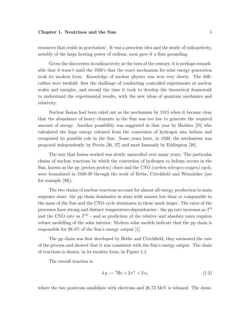
The way that fusion worked was slowly unravelled over many years. The particular
chains of nuclear reactions by which the conversion of hydrogen to helium occurs in the
Sun, known as the pp (proton-proton) chain and the CNO (carbon-nitrogen-oxygen) cycle,
were formulated in 1938-39 through the work of Bethe, Critchfield and Weizsacker (see
for example [39]).
The two chains of nuclear reactions account for almost all energy production in main
sequence stars: the pp chain dominates in stars with masses less than or comparable to
the mass of the Sun and the CNO cycle dominates in those much larger. The rates of the
processes have strong and distinct temperature-dependencies - the pp rate increases as T 5
and the CNO rate as T 15 - and so prediction of the relative and absolute rates requires
robust modelling of the solar interior. Modern solar models indicate that the pp chain is
responsible for 98.4% of the Sun’s energy output [1].
The pp chain was first developed by Bethe and Critchfield; they estimated the rate
of the process and showed that it was consistent with the Sun’s energy output. The chain
of reactions is shown, in its modern form, in Figure 1.1.
The overall reaction is
4 p → 4He + 2 e+ + 2 νe (1.2)
where the two positrons annihilate with electrons and 26.73 MeV is released. The domi-

Chapter 1. Neutrinos and the Sun 6
nant neutrino producing reaction is
p + p → 2H + e+ + νe (1.3)
which produces pp neutrinos with an end point energy of 0.42 MeV. Less numerous are
the mono-energetic pep neutrinos produced in
p + e− + p → 2H + νe (1.4)
Both of these reactions have deuterium in the final state, which takes part in further
reactions and leads the pp chain to one of four terminations. The most probable PPI
chain produces no further neutrinos. The next most probable is the PPII chain, which
produces mono-energetic 0.384 MeV or 0.862 MeV 7Be neutrinos via
7Be + e− → 7Li + νe (1.5)
followed by the PPIII chain, which gives 8B neutrinos ; these have an end point energy of
15 MeV and are produced following the β+-decay of 8B produced in
7Be + p → 8B + γ (1.6)
The least probable termination results in hep neutrinos with energies of up to 18.77 MeV
via3He + p → 4He + e+ + νe (1.7)
The CNO cycle was independently discovered by Bethe and Weizsacker in 1938.
They realised that if other chemical elements were present in a star at its formation - that
it was not composed initially of only hydrogen and helium - then other energy-producing
reactions were possible. They engaged in systematic investigations and came across the
remarkable CNO cycle. As in the pp chain four protons are converted into an alpha
particle with the release of 26.73 MeV, but the path taken is very different. The CNO
cycle uses 12C as a catalyst: the isotope converts, in turn, into 13N, 13C, 14N, 15O, 15N,
and then back to 12C, making a closed loop. Two low energy neutrinos are produced in
this cycle.
1.1.2 Modelling the Sun
The task of building a coherent model of the Sun, suitable for predicting neutrino fluxes, is
much more involved than identifying the energy generation mechanism. The Sun must be
described as a whole, including radiation transport, material transport, thermodynamic

Chapter 1. Neutrinos and the Sun 7
p + p H + e +2 +
ue
99.6 %
p + H +2
uee + p-
0.4 %pp pep
2H g+ p He +
3
3 4 +He + p He e ++ ue
7 8Be + B +p g
8 8 * +B Be e ++ ue
8 *Be 2 He
4
3 4 7He He Be+ + g
2 He He3 4
+ 2 p
7 -Be e+ Li +
7ue
7 4Li 2 He+ p
hep
85 % << 1 %
99.9 % 0.1 %
BPPIII
87Be
PPII
15 %
PPI
Figure 1.1: The pp chain.

Chapter 1. Neutrinos and the Sun 8
Table 1.1: Important solar parameters (from [1]).
Parameter Value
Photon luminosity (L⊙) 3.86 × 1026 J s−1
Neutrino luminosity 0.023 L⊙
Mass (M⊙) 2.0 × 1030 kgRadius (R⊙) 696 000 kmAge ∼ 4.55 × 10⁹ yEffective surface temperature 5.78 × 10³ KCentral temperature 15.6 × 10⁶ KInitial helium abundance by mass (Y) 0.27Initial heavy element abundance by mass (Z) 0.020
behaviour and variations in chemical composition, subject to boundary conditions in space
and time.
The standard approach is to model the development of the Sun since its formation,
subject to constraints on its initial composition and to the requirement that the model
reproduce the current, observable properties of the Sun. The physical processes that gov-
ern stellar evolution are well understood in principle and the considerable sophistication
of solar models is due to the numerical techniques they employ. The uncertainties in their
predictions are mainly due to uncertainties on input parameters.
This section gives an overview of the main components of a solar model: the equa-
tions of stellar evolution, input parameters, boundary conditions, and calculational tech-
niques. A more detailed discussion can be found in the book by Bahcall [1]. The most
recent results from the widely-respected Bahcall model can be found in [2].
The equations of stellar evolution
The Sun is a main sequence star with a radius of 696 000 km and a mass of 2.0× 1030 kg.
Some of its important properties are given in Table 1.1.
Its gross structure can be divided into distinct regions as a function of radius: a
dense, hot inner core, where nuclear fusion occurs; the radiation zone, in which radiative
energy transfer dominates; the convection zone, in which convective energy transfer dom-
inates; the opaque photosphere, in which the Sun’s visible light is produced; and beyond
this, a low density atmosphere.
Solar models begin with the basic equations of stellar evolution, which can be written

Chapter 1. Neutrinos and the Sun 9
as follows, under the good assumption of spherical symmetry:
• Hydrostatic equilibrium.dP
dr= −GMρ
r2(1.8)
where G is the gravitational constant, P and ρ are the pressure and density, re-
spectively, at a radius r, and M is the mass enclosed within r. This relationship
expresses the fundamental balance between gravity and the pressures due to radia-
tion and matter that resist collapse. The sun is treated as a quasistatic system.
• Mass continuity.dM
dr= 4πr2ρ (1.9)
reflects the conservation of mass.
• Luminosity gradient.dL
dr= 4πρε (1.10)
where L and ε are the luminosity and the energy generation rate, respectively, at a
radius r. The luminosity is defined as the radiative energy per unit time through a
sphere at radius r. This equation reflects conservation of energy; the flux of energy
generated by nuclear reactions in the solar core follows the temperature gradient
outwards in radius. Neglecting convection and small contributions from mechanical
energy generation (for example, gravitational contraction) the observed luminosity
is given by
L⊙ =
∫ R⊙
0
dL
drdr (1.11)
where R⊙ is the solar radius.
• Temperature gradient.dT
dr= − 3κLρ
16πσcr2T 3(1.12)
where κ is the opacity, σ is the Stefan-Boltzmann constant and T is the temperature.
This equation describes radiation transport, which is the dominant energy transport
mechanism in all but the outer regions of the Sun.
These equations are accompanied by the equations of state, which express the pres-
sure, opacity and energy generation rate as functions of density, temperature and chemical
composition.

Chapter 1. Neutrinos and the Sun 10
Figure 1.2: The radial production profile of pp chain neutrinos [1].
More refined models also include machinery for dealing with diffusion, in particular
the gravitational settling of heavier elements such as 7Li, and convection in the Sun’s
outer regions.
Input parameters, boundary conditions and calculational procedure
The main boundary condition that must be satisfied by Eq. 1.8 to 1.12 is the outer radial
boundary condition, which is relatively unimportant for processes occurring in the solar
core, such as neutrino production. This is rather fortuitous as the outer regions of the
Sun are those most strongly affected by convection and turbulence, which are difficult
to model. The typical approach is to assume convective equilibrium and the standard
relationships between pressure and temperature that apply in this regime.
The initial chemical abundances are taken from two sources: spectroscopic measure-
ments of the photosphere and of CI carbonaceous chondrite meteorites, which are known
to be representative of the matter from which the solar system formed. Abundances
from both sources are in excellent agreement [40]. In solar models the abundances are
parametrised by three numbers: X, the mass fraction of hydrogen; Y , the mass fraction
of helium; and Z, the mass fraction of elements heavier than helium. The ratio Z/X is
one of the most important parameters. The parameter Y is difficult to measure and it is
left as an adjustable parameter.
Radiative opacities determine the rate of energy transfer from the core to the outer
regions of the Sun and calculating them is extremely complex. It requires a knowledge

Chapter 1. Neutrinos and the Sun 11
Figure 1.3: The predicted solar neutrino energy spectrum [2] showing pp (solid lines) andCNO neutrinos (dashed lines).
of the relative chemical abundances and a detailed simulation of the relevant statistical
mechanics and atomic physics. Calculating solar opacities is a peaceful application of
codes built originally for simulating nuclear weapons.
Nuclear reaction cross sections are the final important ingredient. Typical nuclear
reactions within the Sun occur between charged particles at keV energies so the domi-
nant mechanism is quantum mechanical tunnelling. The cross section for this process is
conventionally parametrised by
σ(E) =S(E)
Eexp(−2πη) (1.13)
where η is the Somerville parameter
η =zZe2
~ν. (1.14)
The term exp(−2πη), known as the Gamow penetration factor, is responsible for reducing
many nuclear fusion cross sections to levels un-measurable in the laboratory at low solar
energies (and consequently for ensuring the slow hydrogen burn rate and long life of
the Sun). Experimental measurements are limited to the 100 keV scale but, because of
the form of Eq. (1.14), can be scaled down in energy with reasonable precision; S(E)
is expanded as a Taylor series and the coefficients fit to the experimental data. Recent
measurements by the LUNA collaboration, using an underground accelerator to reduce

Chapter 1. Neutrinos and the Sun 12
backgrounds, have made the best low energy measurements of a number of reactions, in
particular 3He(3He,2p)4He [41] and d(p,γ)3He [42].
Solar models begin with a main sequence star of homogeneous composition and
evolve it forward in time, typically in steps of 1 × 10⁹ years, until the current age of the
Sun is reached. There are usually two free parameters - the He mass fraction Y and an
initial entropy-like variable - that are iterated until an accurate description of the current
Sun is reached, meaning values of M⊙, L⊙ and R⊙ differing from their present values by
typically less than 1 part in 105.
The primary outputs of solar models are the current solar temperature profile, den-
sity profile, and chemical composition. These outputs can be used to predict the rate of
the nuclear reactions in the core, in particular the relative rates of the different branches of
the pp chain, from which predictions for the observed neutrino fluxes and energy spectra
can be made. Figure 1.2 shows a radial neutrino production profile and Figure 1.3 shows
a flux and energy spectrum prediction.
Helioseismology
The basic test of a solar model is its ability to converge to a state matching the current Sun
in all of its observable parameters, but particularly mass, radius, luminosity and neutrino
flux. It is important to note, though, that aside from comparison of these quantities,
there is a further, very effective way of testing solar models called helioseismology, which
is the study of the propagation of pressure waves within the Sun.
Pressure waves are produced by the turbulence in the convection zone and par-
ticular frequencies are amplified by constructive interference as they propagate between
the boundaries of the convection zone with the radiation zone and the photosphere - the
Sun acts as a resonant cavity. The frequencies of the modes are sensitive to the internal
composition of the Sun, which makes compositions of measured and predicted oscillation
frequencies very instructive. Figure 1.4 shows the radial dependence of the speed of sound,
which can be inferred from the oscillation frequencies, and the excellent agreement with
theory - the predicted and measured speeds agree to better than 0.1% between 0.05 and
0.95 R⊙.
Helioseismology provides tests of many important parameters and, as such, is an
invaluable tool for solar modellers. Its integration over the physics of the solar interior
allows strong constraints to be placed on the rates of the dominant nuclear reactions but
the relative rates of others can be changed with little effect on the oscillation frequencies.

Chapter 1. Neutrinos and the Sun 13
Figure 1.4: Agreement between sound speeds calculated using standard solar models(dashed line) and those measured helioseismologically [3].
1.2 The physics of massive neutrinos
1.2.1 Neutrinos and the standard model
The standard model of particle physics is a unified mathematical description of the elec-
tromagnetic, weak and strong interactions of the known elementary particles. The ele-
mentary particles are spin-1/2 fermions, which interact via the exchange of force carrying
bosons. They are arranged in three generations, each consisting of two oppositely charged
quarks, a charged lepton and neutrino.
Before the discovery of neutrino mass, a massless neutrino was present in each gen-
eration as the left-handed, uncharged partner of the left-handed charged lepton. Each
left-handed doublet was accompanied by a right-handed charged lepton singlet. Experi-
ment dictates that weak interactions couple only to νL and νR and this is reflected in the
structure of the model.
To allow for neutrino mass, modifications are required to the minimal standard
model as a non-zero neutrino mass is inconsistent with the particle’s status as a Dirac
particle existing in one helicity state - masses generated by the Higgs field involve both
helicity states. There are two ways in which the model can be extended: by adding a
right-handed Dirac neutrino state or by treating the neutrino as a Majorana particle,

Chapter 1. Neutrinos and the Sun 14
meaning that it is its own anti-particle.
If the neutrino is a Dirac particle, as all charged fermions must be to conserve electric
charge, then extra right-handed neutrino and left-handed anti-neutrino states must be
added to each generation. The results of experiments, expressed in the basic symmetry
of the standard model, dictate that these extra states must be sterile: to preserve the
basic SUC(3) × SUL(2) structure, right-handed neutrinos would have to be singlets with
respect to weak interaction and therefore be unable to interact weakly.
If the neutrino is a Majorana particle then it is its own anti-particle; the states νL
and νR would be left-handed and right-handed states of the same particle. Majorana
particles fit elegantly into generalisations of the standard model, where they take part in
a see-saw mechanism, which can be used to explain the small neutrino mass scale.
1.2.2 Mixing
Whether neutrinos are Dirac or Majorana particles, it has been established that the weak
eigenstates, in which neutrinos are produced, differ from the mass eigenstates, which gov-
ern their propagation. This difference generates the phenomena of neutrino oscillations:
a neutrino produced in a given flavour eigenstate has a finite probability of being detected
as a different flavour at a different time or point in space.
The neutrino flavour eigenstates να (α = e, µ, τ) can be written in terms of the mass
eigenstates νi(i = 1, 2, 3)
|να〉 =∑
i
Uαi |νi〉 (1.15)
where Uαi is the Pontecorvo-Maki-Nakagawa-Sakata (PMNS) matrix. The nine parame-
ters in this unitary matrix can be expressed in terms of 3 mixing angles and 1 CP-violating
phase.
It is instructive, and often useful, to consider the mixing between two neutrino
generations, say between electron and muon neutrinos. In this case the matrix U depends
only on a single parameter and can be written
U =
(
cos θ12 sin θ12
− sin θ12 cos θ12
)
(1.16)
such that
|νe〉 = cos θ12 |ν1〉 + sin θ12 |ν2〉 (1.17)
|νµ〉 = − sin θ12 |ν1〉 + cos θ12 |ν2〉 (1.18)

Chapter 1. Neutrinos and the Sun 15
The mass eigenstates are stationary states and therefore have a time dependence given
by
|ν1(t)〉 = e−iE1t |ν1(0)〉 (1.19)
|ν2(t)〉 = e−iE2t |ν2(0)〉 (1.20)
Now suppose there is a source of electron type neutrinos at (x, t) = (0, 0) of fixed energy
E. The probability for finding the neutrino to still be electron type at a time t after its
production is given by
P (νe → νe) = |A(νe → νe)|2 = |〈νe|νe(t)〉|2 (1.21)
where
|νe(t)〉 = cos θ12e−iE1t |ν1(0)〉 + sin θ12e
−iE2t |ν2(0)〉 (1.22)
At all practical energies neutrinos are highly relativistic so p ≫ mi and E ∼ p, and Ei
can be written
Ei =√
p2i + m2
i ≃ pi +m2
i
2pi≃ E +
m2i
2E(1.23)
so Eq. (1.22) becomes
|νe(t)〉 = e−iE1t
(
cos θ12 |ν1(0)〉 + sin θ12ei∆m2
12t
2E |ν2(0)〉)
(1.24)
where ∆m212 = m2
1 − m22. After some algebra, the probability P can then be written
P (νe → νe) = 1 − sin2 2θ12 sin2
(
∆m212L
4E
)
(1.25)
where t has been replaced by L, which is the distance from the source to the measuring
point. P (νe → νe) is referred to as the survival probability.
Examining Eq. (1.25) it can be seen that the survival probability oscillates with a
characteristic length
L =4πE
∆m212
which is the distance travelled by the neutrino before it returns to its initial state i.e.
until the point where the probability of measuring it to be an electron neutrino is 1. The
mixing angle θ12 determines the oscillation amplitude and the mass squared difference
sets the oscillation length.
If the neutrino source has dimensions comparable to or larger than L, or produces
neutrinos with a range of energies, then the average survival probability is given by
P (νe → νe) = 1 − 1
2sin2 θ12
The maximum suppression is therefore 1/2.

Chapter 1. Neutrinos and the Sun 16
1.2.3 Matter enhancement
The considerations above apply to oscillations in vacuum, but if the neutrinos travel
through a dense medium then the situation becomes more complex as propagation is
affected by interactions with the medium. These interactions are not the same for all
neutrinos flavours: electron neutrinos can scatter from electrons via the CC and NC
interactions but muon and tau neutrinos can scatter only via the NC interaction. This
difference in potential affects the flavour composition of a neutrino beam and is known at
the MSW effect after Wolfenstein [43] who discovered it and Mikhaev and Smirnov who
applied it to solar neutrinos [44].
Consider the case of two flavour mixing, but this time in the presence of a uniform
medium. Electron neutrinos experience an additional potential Vw in their Hamiltonian,
compared to muon and tau neutrinos, which alters their forward scattering amplitude.
The weak potential Vw is given by
Vw = GF
√2Ne (1.26)
where Ne is the electron density. This is equivalent to an extra effective mass so that m2
becomes
m2 = (E + Vw)2 − p2 ≃ m2 + 2EVw (1.27)
Thus, the mass squared of the electron neutrino increases by
2√
2GFNeE (1.28)
The algebra from the previous section can be repeated with Vw included. The
Schrodinger equation for the propagation of the flavour states is
id
dt
(
νe
νµ
)
= M
(
νe
νµ
)
(1.29)
where M is the mass matrix. For propagation in vacuum, M can be written
MV =∆m2
4p
(
− cos 2θ sin 2θsin 2θ cos 2θ
)
(1.30)
where terms giving the same phase factor to both flavours are neglected. For propagation
in matter, M is given by
MM =∆m2
4p
(
− cos 2θ + A sin 2θsin 2θ cos 2θ − A
)
(1.31)
where A = 2√
2GFNep/∆m2. If a matter mixing angle θm is defined such that

Chapter 1. Neutrinos and the Sun 17
Figure 1.5: The MSW effect, for a small vacuum mixing angle [4]. The masses of the νe
and νµ flavour eigenstates as a function of solar radius (light lines). The top dark lineshows the development of a νe as it leaves the production point in the solar core andconverts into a νµ.
∆m2
4p
(
− cos 2θ + A sin 2θsin 2θ cos 2θ − A
)
=∆m2
m
4p
(
− cos 2θm sin 2θm
sin 2θm cos 2θm
)
(1.32)
then matter and vacuum mixing angles are related by
tan 2θm =sin 2θ
cos 2θ − A=
tan 2θ
1 − (Lν/Lm) sec 2θ(1.33)
where the vacuum oscillation is Lν = 4πp/∆m2, as before, and the electron interaction
length is Lm = 4π/(2√
2GF Ne), so that A = Lν/Lm. Regardless of the value of θ, as long
as ∆m2 > 0 (i.e. m2 > m1) a resonance can occur at an electron density equal to
Ne = ∆m2 cos 2θ12
2√
2GFp(1.34)
at which point the mixing becomes maximal.
Figure 1.5 shows the effect of this mechanism in the Sun where the electron density
varies as a function of radius. This schematic figure applies to the situation where the
vacuum mixing angle is small. The figure shows νe and νµ masses as a function of radius:
the νµ mass is independent of electron density and is represented by a straight line, while
the νe mass is proportional to electron density. At the resonance, where θm = π/4, the νe
has a mass that in vacuum would be largely identified with the νµ flavour eigenstate. It can
be shown (see [1]) that, as long as the electron density changes slowly and adiabatically,
transitions between the mass states ν1 and ν2 are suppressed and when the neutrino exits
Chapter 1. Neutrinos and the Sun 18
the Sun in remains mostly ν2; in the diagram the νe produced in the solar core follows
the solid line and leaves the Sun as a νµ.
In the Sun the resonance condition is not met for low energy neutrinos and their
behaviour is governed by vacuum oscillations. However, for higher energy neutrinos it can
be met and results in greater suppression of the electron neutrino flux than possible with
vacuum oscillations alone [4]. It can be shown [45] that the average survival probability
in the presence of a matter oscillation resonance becomes
PMSW (νe → νe) =1
2+
(
1
2− Pjump
)
cos 2θm cos 2θ12 (1.35)
where θm is determined using the density at the νe production point and Pjump is the
probability of jumping from one adiabatic mass state to the other, which is small because
of the slowly changing electron density in the Sun. In contrast to the equivalent expression
for vacuum oscillations (Eq. (1.2.2)) the minimum value of this expression can approach
0, rather than 1/2, making it a more powerful suppression mechanism.
The smoking gun signature for matter oscillations, as opposed to vacuum oscilla-
tions, is the characteristic energy dependence; the relatively larger suppression of neutrinos
with enough energy to pass through resonance compared to those of lower energy. This
can be observed by comparing the suppressions observed in experiments with different en-
ergy thresholds or by looking for distortions to the energy spectra of neutrinos produced
with a continuous energy distribution. The former has been observed over the range of
solar neutrino experiments but no measurement has yet been made of matter-induced
spectral distortions.
A further signature for matter oscillations is the so-called day-night effect in which
the solar neutrino flux measured during daytime differs from that measured during the
nighttime, when the neutrinos have to pass through the additional mass of the Earth.
During the night, the neutrino beam can be regenerated by the inverse of the process
occurring in the Sun. This process, whereby a νµ can be converted into a νe is illustrated
in Figure 1.5. It is predicted to be a small effect and has not yet been observed.
1.3 Evidence for neutrino mass and oscillations
1.3.1 Oscillation parameters
In three flavour neutrino mixing, the matrix U , which connects the flavour and mass
eigenstates, can be factorised as

Chapter 1. Neutrinos and the Sun 19
U =
1 0 00 c23 s23
0 −s23 c23
·
c13 0 s13 e−iδ
0 1 0−s13 eiδ 0 c13
·
c12 s12 0−s12 c12 0
0 0 1
(1.36)
where sαi = sin θαi, cαi = cos θαi, θαi is the mixing angle and δ is the CP-violating
phase. This form is convenient because, experimentally, θ13 is found to be small and
∆m223 ≫ ∆m2
12, meaning that mixing in the θ12 ‘solar sector’ and the θ23 ‘atmospheric
sector’ can be approximated by two flavour oscillations, as described in the previous
sections.
A full characterisation of the neutrino oscillation phenomena requires measurements
of the four parameters in the matrix and the mass squared differences ∆m212 and ∆m2
23.
Meaningful measurements have been made of, or limits placed on, all the parameters
except δ. Recent values are
Parameter Value. Main experiment(s) Ref.
tan2 θ12 0.47+0.06−0.05 SNO, KamLAND [5]
sin2 θ23 > 0.95 MINOS [6]sin2 θ13 < 0.19 CHOOZ [46]∆m2
12 7.59+0.21−0.21 × 10⁻⁵ eV2 SNO, KamLAND [5]
∆m223 (2.43 ± 0.13) × 10−3 eV2 MINOS [6]
where uncertainties correspond to 68% confidence level except for CHOOZ which corre-
sponds to 90% confidence level. The limit on sin2 θ13 was quoted using ∆m223 = 1.9×10⁻³
eV2 and would be slightly lower for the value of ∆m223 in the table. The solar sector
mixing parameters do not include the data analysed in this thesis.
The following section describes the measurements of these parameters and of at-
tempts to fix the mass hierarchy (the ordering in mass of the states ν1, ν2, ν3) and scale
(the absolute as opposed to the relative mass scale).
1.3.2 The solar sector
Measurements of θ12 and ∆m212 are dominated by the SNO and KamLAND experiments.
The SNO experiment (described in detail in the next section) measured the total
flux of solar neutrinos above ∼ 5 MeV and its electron neutrino component. The physics
signatures were the ratio of the νe flux to the total neutrino flux (νe + νµ + ντ ) and the
ratio of νe fluxes during day and night. The results of the experiment are consistent with
the primary oscillation mechanism being matter oscillations within the Sun.

Chapter 1. Neutrinos and the Sun 20
Figure 1.6: Contours showing allowed values of the solar sector mixing parameters [5].This plot does not include the results from this thesis.
The observation of a νe to (νe + νµ + ντ ) ratio of less than unity demonstrates that
neutrinos change flavour. Its particular value places a strong constraint on θ12 and non-
observation of a day-night effect, which would have been evidence for matter-regeneration
of the νe flux within the Earth, places a weak constraint on ∆m212. The interpretation of
the νe flux suppression in terms of the MSW effect means that m2 > m1.
The KamLAND experiment detects electron anti-neutrinos from nuclear reactors in
Japan and South Korea. The typical baseline (reactor-experiment separation) is 180 km
and νe neutrinos are detected using the inverse beta decay process
νe + p → e+ + n (1.37)
whose signature is light from annihilation of the e+ and a delayed 2.2 MeV γ from cap-
ture of the neutron by a proton. The active volume is 1000 tonnes of ultra-pure liquid
scintillator contained in a transparent nylon balloon and instrumented with 1879 pho-
tomultiplier tubes. The combination of KamLAND’s average baseline and a νe energy
spectrum extending to ∼ 7 MeV makes the experiment sensitive to vacuum oscillations
in the same region of θ12 − ∆m212 parameter space that SNO is sensitive to via matter
oscillations.
KamLAND [47, 48, 5] observes a deficit in the anti-neutrino flux and a distortion in
the detected neutrino energy spectrum characteristic of vacuum oscillations. There are

Chapter 1. Neutrinos and the Sun 21
θ
Δ
Figure 1.7: Contours showing allowed values for the atmospheric mixing parameters [6].
no matter oscillations because of the short baseline, low energies and low density of the
Earth. KamLAND’s results place a strong limit on ∆m212 and a weaker one on θ12.
If CPT invariance is assumed, so that the neutrino and anti-neutrino oscillation
parameters are identical, then the results of the solar experiments and of KamLAND can
be combined. Figure 1.6 shows the KamLAND and solar results (dominated by SNO)
superimposed and in excellent agreement.
1.3.3 The atmospheric sector
The first direct evidence for neutrino mass was found in the analysis of atmospheric
neutrino data taken by the Super-Kamiokande water Cerenkov detector [49].
Atmospheric neutrinos are produced by interactions of cosmic rays with nuclei in the
Earth’s atmosphere. Copious numbers of pions are produced in these reactions, which
decay to muons and anti-muons with their accompanying neutrinos; additional muon

Chapter 1. Neutrinos and the Sun 22
and electron neutrinos are produced when the muons decay. GeV-range neutrinos are
produced uniformly at the same rate all around the Earth and so the measured upward-
and downward-going fluxes at any point should be equal. Super-Kamiokande found that
this was true for electron neutrinos but not for muon neutrinos, providing evidence that
neutrinos have mass. This was interpreted as being due to their oscillation into tau
neutrinos while passing through the Earth. Analysis of the data allowed ∆m223 and θ23 to
be measured.
In much the same was as KamLAND is able to probe the solar parameter space
using a terrestrially generated neutrino source, so muon-neutrino-producing accelerator
neutrino experiments are able to probe the atmospheric neutrino parameter space. K2K
[50] and MINOS [6] are the most important experiments of this type. Each consists of an
accelerator producing muon neutrinos, a near detector close to the source to characterise
the beam and a far detector, positioned 250 km away for K2K and 735 km away for
MINOS, to characterise the beam after oscillation. Both experiments have observed a
deficit and seen the expected distortion to the energy spectrum. MINOS is a more recent
and higher precision experiment.
Atmospheric and accelerator data can of course be combined to yield the best esti-
mates for θ23 and ∆m223. The results of a recent global analysis are shown in Figure 1.7.
1.3.4 θ13 and CP violation
A parameter of particular importance in the mixing matrix is θ13, which must be non-zero
to allow CP violation to be measured. A measurement of CP violation in neutrinos would
be of immense cosmological interest.
No measurement has yet been made of θ13 but there are two active approaches:
a search for νe disappearance in short baseline reactor neutrino experiments and νe or
νe appearance in a long baseline accelerator neutrino experiment. A measurement of a
sufficiently large θ13 would motivate the construction of a neutrino factory, which is a
high-intensity neutrino source using muon-storage rings, that could make a measurement
of the CP-violating phase δ.
1.3.5 Remaining questions
The neutrino mass spectrum has only been partly resolved by existing experiments: mea-
surements in the solar sector yield ∆m212 and establish that m2 > m1 and those in the

Chapter 1. Neutrinos and the Sun 23
atmospheric sector determine ∆m223. That leaves two pieces of information missing: the
ordering of the ν2 and ν3 mass states - to establish the mass hierarchy - and the absolute
mass of one of the neutrinos.
The mass hierarchy can be established from the study of the matter interactions of
accelerator neutrinos. The absolute mass scale may be determined by the study of the β
energy spectrum end point in tritium β decay, by measuring the effective Majorana mass
in double beta decay, or from cosmological models. The strongest constraint is currently
provided by the latter - [51] calculate a limit on the sum of the neutrino mass states of
0.17 eV at 95% confidence level.

Chapter 2
Measuring the flux of solar neutrinos
The first principle is that you must not fool yourself - and you are the easiest
person to fool.
RICHARD FEYNMAN (1974)
2.1 The three phases of SNO
The SNO experiment used a heavy water target to detect 8B solar neutrinos. The use
of heavy water gave SNO the unique ability to measure both the total flux of solar
neutrinos and its electron neutrino component. The experiment was proposed by Herb
Chen [52] in 1984.
Neutrinos interact with heavy water in three ways, which are illustrated in Fig-
ure 2.1. They are
νe + d → p + p + e− − 1.44 MeV (2.1)
νx + e− → νx + e− (2.2)
νx + d → p + n + νx − 2.22 MeV (2.3)
where the symbol νx refers to any neutrino flavour.
The charged-current (CC) interaction (Eq. 2.1) is sensitive only to electron-type
neutrinos and its signature was the Cerenkov light produced by the final state electron.
The threshold is 1.44 MeV and there is a weak correlation between the directions of the
24

Chapter 2. Measuring the flux of solar neutrinos 25
�W
D
νe
p
p
e−
(a) Charged-current
�Z0
D
νx
p
n
νx
(b) Neutral-current
�W
e−
νe
νe
e−
�Z0
e−
νx
e−
νx
(c) (d)Elastic scattering
Figure 2.1: Diagrams of the neutrino interactions in SNO. Adapted from [7].

Chapter 2. Measuring the flux of solar neutrinos 26
electron and neutrino; the distribution of angles is given by
f(cos θ⊙) ≃ 1 − 1
3cos θ⊙ (2.4)
where θ⊙ is the angle between the directions. There is a correlation between the electron
and neutrino energies.
The elastic-scattering (ES) interaction (Eq. 2.2) is sensitive to all neutrino flavours,
though preferentially to νe, by a factor of ∼ 6 at solar neutrino energies compared to its
sensitivity to νµ or ντ . This is because electron neutrinos can scatter via both W and
Z0 exchange whereas muon and tau neutrinos are restricted to the latter. The signature
was again a final state Cerenkov electron and events were distinguished from CC events
by the strong correlation between the neutrino and electron directions, which generates
a sharp peak in the distribution of electron directions, pointing away from the Sun. At
SNO energies the ES cross section is approximately 10 times smaller than CC, making
this a minor interaction.
The neutral-current (NC) interaction (Eq. 2.3) is equally sensitive to all neutrino
flavours. It has a threshold of 2.2 MeV and its signature was the production of the
final state neutron. There was no correlation between the properties of the detected
neutron and the neutrino - all energy and direction information was lost because neutrons
scattered many times and thermalised before capture. The neutrons were counted via a
different mechanism in each phase of the experiment: in the first phase using the gamma
produced following capture back on a deuteron; in the second phase using the gamma
cascade produced following capture on 35Cl, introduced into the detector in the form
of common salt; and in the third phase by capture on 3He in an array of proportional
counters anchored in the heavy water. The three phases are described in the following
sections, after a brief description of the detector.
The detector is shown in Figure 2.2. It was designed and instrumented primarily
to detect Cerenkov light from CC, ES and NC interactions in the heavy water - CC and
ES from the final state electrons and NC from Compton-scattered electrons produced in
(n,γ) reactions.
The target was 1000 tonnes of heavy water contained in a transparent acrylic vessel
(AV) of diameter 12 m and thickness 5.5 cm, suspended by ropes from a deck structure
at the top of the cavity. The AV had a cylindrical neck, or chimney, of diameter 1.5 m
allowing access to the heavy water for deployment of calibration sources. Outside the
AV was a region of ultra pure light water shielding and beyond that an array of 9456
20 cm photomultiplier tubes (PMTs), which were fixed to a 17.8 m diameter geodesic
steel structure. Between the structure and cavity walls was a further region of light water

Chapter 2. Measuring the flux of solar neutrinos 27
InnerH O2
D O2
OuterH O2
NCDString
AcrylicVessel
PSUP
Figure 2.2: The SNO detector. Adapted from [8].

Chapter 2. Measuring the flux of solar neutrinos 28
acting as both a shield from radioactivity in the rock and as a muon veto. The AV had
transparent acrylic anchor blocks arranged on a grid in the lower half of the detector to
anchor the proportional counters in the final phase of the experiment.
The detector was located at a depth of 2092 m (5890±200 m water equivalent [53])
in the Creighton Nickel Mine in Sudbury, Canada. At this depth the cosmic ray muon
flux is highly attenuated and only ∼ 70 muons interacted in the heavy water per day.
Water purification systems maintained low levels of U, Th (and their daughters) in
the light and heavy water and strict material selection procedures ensured very low levels
in the fixed materials.
2.1.1 The D2O phase
In the first phase of the experiment [54, 55], which ran from November 2, 1999 to May
31, 2001, neutrons were detected using the reaction
n + d → t + γ + 6.25 MeV (2.5)
in which a neutron captured on a deuteron producing a single 6.25 MeV gamma in the final
state. The gamma typically Compton scattered an electron and the resultant Cerenkov
light was detected.
This phase provided a precise measurement of the CC flux. The NC measurement
was more limited, for two reasons: the first was the difficulty in distinguishing the CC
electron from the Compton-scattered NC electron - in a fit, making no assumption on the
neutrino energy spectrum, the only distinguishing observables were radius and direction
from the Sun, in which CC and NC events did not differ strongly; the second was the low
d(n,γ) cross section of 0.5 mb, which gave a neutron detection efficiency of only 14.4%,
and correspondingly low statistics. It was possible to make a measurement of the NC
flux using only radius and direction from the Sun as observables, but to made a good
measurement the neutrino energy spectrum had to be assumed and energy used as an
additional distinguishing variable.
2.1.2 The Salt phase
In the second phase of the experiment [9], which ran between July 26, 2001 and August
28, 2003, 2 tonnes of NaCl were added to the heavy water to improve the neutron response

Chapter 2. Measuring the flux of solar neutrinos 29
Figure 2.3: Results from the salt phase [9]. The plot shows the flux of muon + tauneutrinos versus the flux of electron neutrinos.
of the detector. Neutrons were detected using the reaction
n + 35Cl → 36Cl + γs + 8.6 MeV (2.6)
in which the neutron captured on 35Cl emitting a cascade of gammas with a total energy
of 8.6 MeV.
The addition of salt increased the neutron detection efficiency (to 41%) because of
the large 35Cl(n,γ) cross section of 44 b. It also allowed CC and NC events to be more
easily distinguished: the gamma cascade produces multiple Compton-scattered electrons
and therefore Cerenkov light that is more isotropic than that produced by a single CC
electron. A good measurement of the NC flux could be made with no assumption on the
neutrino energy spectrum. The results are shown in Figure 2.3.
2.1.3 The NCD phase
In the third phase of the experiment the salt was removed and an array of 3He proportional
counters, known as NCDs (neutral-current detectors), were deployed in the heavy water.
Neutrons were detected using the reaction
n + 3He → p + t + 764 keV (2.7)
There were three main reasons for changing the neutron detection mechanism so radically
from the first two phases:

Chapter 2. Measuring the flux of solar neutrinos 30
• The CC-NC correlation was broken.
In the salt and D2O phases there was a significant correlation between the CC and
NC fluxes, which arose because of the large overlap of the distributions in each of
the observables. In the NCD phase the correlation was much reduced because the
CC and NC events were recorded in effectively independent detectors - CC events
in the PMT array and NC events mainly in the NC array. These are the salt and
NCD phase correlation matrices:
Salt phase NCD phase
CC ES NC CC ES NC
CC 1.00 CC 1.00ES -0.16 1.00 ES 0.24 1.00NC -0.52 -0.06 1.00 NC -0.19 0.02 1.00
• The systematics on the NC flux were different.
The systematic uncertainties associated with the NC measurement were substan-
tially different to previous phases. SNO was a systematics-limited experiment and
the exchange of one set of systematics on the NC flux for another was an extremely
powerful check that the estimates for both sets of systematic uncertainties were
robust.
• Neutron contamination of the CC spectrum was diminished.
NC neutron events were the largest background to the CC signal in the first two
phases but in the NCD phase they were greatly reduced in number: the ratio of
NC to CC PMT events in the NCD phase was ∼ 0.14 compared to ∼ 0.92 in the
salt phase. The benefit of this reduction in ‘background’ was somewhat offset by
the interference of the NCD array with the detection of Cerenkov light but, even
accounting for this, it was possible to make a measurement of the CC flux with
comparable precision to previous phases. Note that the energy threshold was higher
than in previous phases so the measurement necessarily provided less information
on the CC (and therefore 8B neutrino) energy spectrum.
The challenges of the NCD phase were accounting for the shadowing and reflection of
Cerenkov light by the counters, handling the radioactivity introduced into the detector
in the materials of the array, and identifying neutron events in the counters above the
background of instrumental and radioactive backgrounds.

Chapter 2. Measuring the flux of solar neutrinos 31
2.2 Detecting neutrons
2.2.1 The NCD array
The NCD array was an array of 3He proportional counters which detected neutrons via
the reaction
n + 3He → p + t + 764 keV
and recorded the ionisation produced by the final state proton and triton. Such counters
are widely used for neutron detection, but the design of an array suitable for use inside
the target of a low background Cerenkov detector presented unique challenges. The array
had to have the following properties:
• high neutron capture efficiency,
• geometry causing minimal interference with Cerenkov light from CC reactions,
• low radioactive contamination to minimise the background to the NC signal from
ionisation due to alphas produced inside the counters and neutrons produced by
photodisintegration of deuterons external to the counters,
• provide sufficient information on the characteristics of the ionisation to allow neutron
events to be distinguished from instrumental events and those due to radioactivity,
• mechanical stability over long periods of time in the large pressures at the bottom
of the heavy water and in an environment subject to seismic disturbances.
The need for a high capture efficiency and small interference with Cerenkov light fixed the
basic geometry of the array, which consisted of long, thin counters sparsely distributed
throughout the heavy water. The high 3He neutron capture cross section of 5316 b meant
that the counters, with a diameter of 5 cm, remained effectively black to neutrons.
The need for low backgrounds required that the amount of material added to the de-
tector be minimised, that the material added have as small an amount of radioactive con-
tamination as possible, and what contamination there was be accurately measured. The
nickel counter walls, in particular, were made extremely thin; specialist low-background
processes were used to produce the bodies; and the long periods of underground storage
prior to deployment used to allow cosmogenic activity to decay away.
The ability to separate events due to neutrons from backgrounds required a combi-
nation of gas properties and counter radius such that ionisation from typical events was

Chapter 2. Measuring the flux of solar neutrinos 32
I1
x
y
I1 K3 M3 N2 M6 K6 I1N3
M5
K5 J5
L3 J6
K7
J7
I1M7
J8
L2M8
N4
K8
I1I1
K1
M1
N1
L1
M2
J1
J2
J3
K2
L4 M4
K4
I1 I1
J4
3He
4He
Figure 2.4: The NCD array looking down into the detector in the negative z direction.
contained within the counters - that the probability of particles colliding with the walls
be minimised. Pulses were digitised to allow comparison of the energy deposition profiles
between different pulses. Some counters were filled with 4He rather than 3He to allow the
study of backgrounds; the radiation transport properties of the two gases are identical
but 4He could not capture neutrons.
Each NCD was a string of 3 or 4 counters laser-welded together in series. Strings
were buoyant and were anchored to fixtures built into the acrylic vessel. Signals were
read out from strings via cables leaving the tops of the strings and exiting the detector
through the AV neck. The cables were attached to the anode wires using flexible resistive
couplers.
The geometrical arrangement of the NCDs is shown in Figure 2.4. Cartesian and
spherical coordinates systems were defined with respect to an origin at the centre of the
PSUP, which approximately coincided with the centre of the AV. In the Cartesian system
the z-axis is vertical and parallel with the NCDs. The only spherical coordinate used in
this thesis is r = (x2 + y2 + z2)1/2.
The NCDs were positioned on a 1 m grid; in the xy-plane they were clustered
towards the centre of the detector, though vertically they extended to within 10s of cm

Chapter 2. Measuring the flux of solar neutrinos 33
of the AV. The clustering in the xy-plane was to reduce the length of the cables (and
therefore the amount of associated U and Th in the detector) and to optimise the neutron
detection efficiency.
The array geometry was originally optimised for a measurement of 1/3 of the stan-
dard solar model rate, which called for a 96 string arrangement. However, given the strong
indication from the first two phases that the NC flux was consistent with expectations
the array could be reduced to 40 strings comprising 156 individual counters and 398 m of
active length.
A diagram of an NCD string is shown in Figure 2.5. The average wall thickness was
∼ 400 µm and the copper anode wire had a diameter of 50 µm. The counter gas was a
mixture of 85% 3He or 4He by pressure with 15% CF4 at a pressure of 2.50 ± 0.01 atm.
The 3He density was 1.07 × 10⁻⁴ g cm−3.
The nickel used in the counters was produced in a chemical vapour deposition (CVD)
process. The process began with a source of nickel which was heated in a carbon monoxide
atmosphere. Under pressure at ∼ 50 C nickel combines with carbon monoxide to form
gaseous Ni(CO)4, a process which reverses at ∼ 175 C. Using this cycle nickel could be
extracted from the source and deposited onto cylindrical mandrels with diameters equal
to the inner diameters of the counters. The nickel was purified because, while U and Th
also form carbonyls, they do not do so reversibly at these temperatures.
Finished counter bodies were stored underground to allow cosmogenic activity to
decay away and were etched and electropolished to remove any contamination from the
handling and storage processes, in particular the alpha-emitting radon daughter 210Po,
which was discovered on the surfaces in relatively high concentration.
Electrical field lines close to the counter ends were necessarily distorted by the
counter geometry, so fused silica insulators were fitted around the anode wires at these
points to prevent deposited ionisation from being collected. This caused a small reduction
in the active volume of the array - and hence in the neutron detection efficiency - but
prevented distorted pulses, which would have been difficult to model, from entering the
data steam.
Strings were installed using a remotely operated vehicle (ROV), which was a custom
built submersible used to guide the NCD anchors into their fixtures.
After deployment, two discrete sources of radioactive contamination were discovered
on strings K2 and K5. Using a variety of methods the composition of these hotspots could
be determined and accounted for in the analysis; the way in which this was done is

Chapter 2. Measuring the flux of solar neutrinos 34
Figure 2.5: An NCD string. Adapted from [8].

Chapter 2. Measuring the flux of solar neutrinos 35
Preamp
Multiplexer
NCD
Oscilloscope
Shaper-ADC
~ 600 sμ
236 s (fixed)μ
0.8 s
Figure 2.6: Schematic diagram showing the main components of the NCD electronics.The numbers in grey indicate the dead time associated with each component.
discussed in detail in Section 8.2.4. Other mechanical defects observed in the array were
a leak of 3He into the counter-interspace region on string K5; permanent or periodic
electrical disconnect due to faulty resistive couplers on strings K2 and M8; and gain
instabilities on string K7.
2.2.2 Data acquisition
The NCD data acquisition system (DAQ) was designed to detect neutrons from two
different sources with very different characteristic event rates: 8B solar neutrinos and
neutrinos from a possible galactic supernova.
A galactic supernova of the magnitude expected every 100 years would have pro-
duced a large burst of neutrons with a kHz event rate, and the number of events and
relative timing would be of immense physical interest. For low rate solar neutrino data
the main issue was the ability to distinguish neutron events from backgrounds and instru-
mentals and, to this end, the detector was required to digitise individual pulses to allow
discrimination based on the energy deposition profiles.
To achieve the goals of high rate data collection and pulse digitisation in a cost
effective manner, a system was designed that had two paths with independent triggers: a
fast pulse integration path with a threshold set on event charge and a slower digitisation
path with a threshold set on pulse amplitude. A simplified diagram of the system is shown
in Figure 2.6.
The pulse integration path is referred to as the shaper-ADC system. Signals were

Chapter 2. Measuring the flux of solar neutrinos 36
integrated by a series of operational amplifiers and compared to a threshold set string-by-
string. There was one shaper-ADC for every 6 or 7 strings and the dead time was fixed
at 236 µs. To verify the dead time each channel was fitted with a scalar counter to count
the number of times the signal crossed the threshold but was not read out.
The digitisation path is referred to as the scope system. The path began in the
multiplexer - one box for up to 12 strings - where signals were log-amplified to help deal
with the large dynamic range. If the pulse passed a given threshold, again set string-by-
string, the multiplexer attempted to digitise the event using one of a pair of oscilloscopes.
If a scope was available it digitised the pulse at a rate of 1 GHz for 15 µs. The dead time
associated with each multiplexer was typically 600 µs and with each scope, 0.8 s.
Events selected for data analysis had to trigger both the shaper-ADC and scope
systems.
2.2.3 Events in the counters
The physics events in the counters were neutron captures and events due to alphas, elec-
trons and gammas from radioactive backgrounds. Alphas were by far the most important
background to the neutron signal.
A neutron capturing in a counter produced a back-to-back proton-triton pair with
total energy 764 keV, which was the maximum amount of energy that could be deposited
as ionisation (the triton and proton carried 191 and 563 keV respectively). The minimum
amount of energy typically deposited in the gas was 191 keV, occurring when the proton
struck the counter wall immediately after being produced. Some of the topologies are
illustrated in Figure 2.9. Both the proton and neutron have Bragg peaks and neutron
events, with suitable geometries, generated characteristic double-peaked pulses.
Alpha events had a single Bragg peak and the pulses were therefore single-peaked.
They ranged in energy up to ∼ 9 MeV and had a spectrum that was featureless in the
neutron region (191-764 keV). Over the whole energy range, the spectrum for U and Th
chain bulk alphas produced within the nickel walls was featureless, but the Po surface
alphas produced a large peak at 5.3 MeV.
Electrons and gammas produced long, low energy pulses that made them easy to
distinguish from neutrons and alphas.
Individually, background neutrons were indistinguishable from signal neutrons be-
cause they typically scattered many times and thermalised before capture. The main pro-

Chapter 2. Measuring the flux of solar neutrinos 37
µµ
µ µ
µµ
Figure 2.7: Example pulses: neutron (top left), alpha (top right), J3 instrumental (bottomleft), and oscillatory noise event (bottom right). In the neutron and alpha panels the redlines are pulses where the ionisation was deposited along a path oriented close to thecounter radius, perpendicular to the wire, and the black lines represent pulses where itwas deposited close to parallel with the wire.
Energy (MeV)0 1 2 3 4 5 6 7 80
500
1000
1500
2000
2500
3000
3500
Figure 2.8: Shaper-ADC energy spectrum for the neutrino data set.
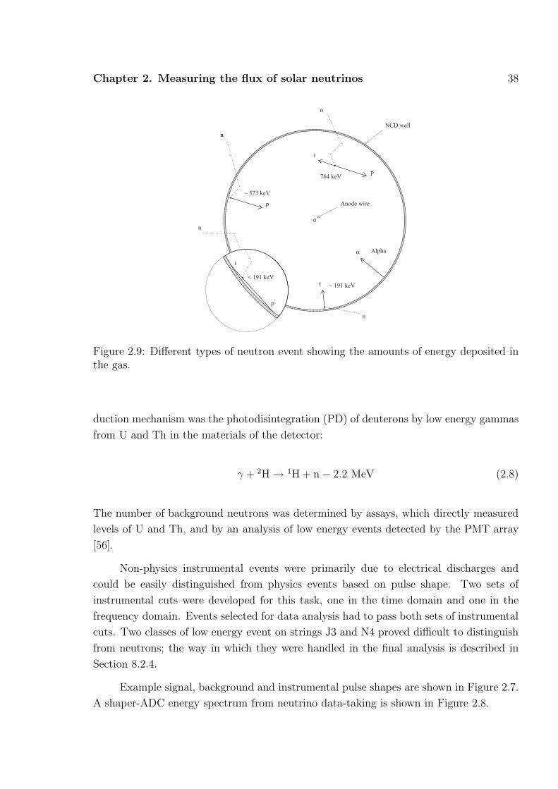
Chapter 2. Measuring the flux of solar neutrinos 38
t
Anode wire
p
NCD wall
764 keV
a Alpha
p
t
t
p
n
n
n
n
n
~ 573 keV
~ 191 keV
< 191 keV
Figure 2.9: Different types of neutron event showing the amounts of energy deposited inthe gas.
duction mechanism was the photodisintegration (PD) of deuterons by low energy gammas
from U and Th in the materials of the detector:
γ + 2H → 1H + n − 2.2 MeV (2.8)
The number of background neutrons was determined by assays, which directly measured
levels of U and Th, and by an analysis of low energy events detected by the PMT array
[56].
Non-physics instrumental events were primarily due to electrical discharges and
could be easily distinguished from physics events based on pulse shape. Two sets of
instrumental cuts were developed for this task, one in the time domain and one in the
frequency domain. Events selected for data analysis had to pass both sets of instrumental
cuts. Two classes of low energy event on strings J3 and N4 proved difficult to distinguish
from neutrons; the way in which they were handled in the final analysis is described in
Section 8.2.4.
Example signal, background and instrumental pulse shapes are shown in Figure 2.7.
A shaper-ADC energy spectrum from neutrino data-taking is shown in Figure 2.8.

Chapter 2. Measuring the flux of solar neutrinos 39
Glove Box
Motor Mounts
Central Rope
ManipulatorCarriage
Source
Side Rope
Figure 2.10: The calibration source manipulator system. Adapted from [8].
2.3 Detecting Cerenkov light
2.3.1 The PMT array
The PMT array consisted of 9456 20 cm photomultiplier tubes custom made for SNO
with low radioactivity glass and components. 9438 of the tubes faced inwards to detect
neutrino events; 91 faced outwards to instrument the light water region, making it an
effective muon veto; 4 were installed in the detector neck to veto events caused by static
discharges in the gas above the heavy water; and 23 were mounted on a removable sled
to allow studies of material ageing.
The tubes facing inwards were fitted into reflective concentrators, which increased
the effective photocathode coverage by ∼ 60%. Magnetic compensation coils built into
the cavity walls cancelled the vertical component of the Earth’s magnetic field, increasing
the collection efficiency by an average of 10%.
Event positions and directions were estimated using a time-of-flight fitter and ener-
gies using a position-dependent conversion applied to the number of hit PMTs.

Chapter 2. Measuring the flux of solar neutrinos 40
2.4 Calibration
2.4.1 Electronics calibrations
Regular electronics calibrations were required for both the NCD and PMT arrays.
For the NCD array there were two classes of calibration: one measured the response
of the electronics and one searched for anomalous behaviour symptomatic of electrical
disconnects at the resistive couplers connecting the anode wires to the cables.
The electronics response calibration was used to determine the linearity of the sys-
tem, to quantify the shaper-ADC and digitisation thresholds and to measure the parame-
ters governing the logarithmic amplification and digitisation of pulses. Electrical pulses of
various shapes were injected into the preamplifier and compared with the recorded pulses
to extract the parameters of interest.
The electrical disconnect calibrations were performed to search for failure of the
resistive couplers. During the NCD phase one string suffered a permanent failure and
another experienced intermittent failure. The disconnects were discovered by the obser-
vation of anomalously long periods where no events were observed in the detectors. To
guard against this behaviour in other strings, on shorter and therefore less noticeable
timescales, a calibration task was implemented that injected a distinctive square pulse
into a preamplifier every minute, and looked for reflected pulses with shapes indicative of
disconnects. None were found on any other strings.
PMT electronics calibrations were used to measure various parameters such as the
discriminator thresholds and timing.
2.4.2 Physics calibrations
Calibration sources were used to determine the response of the NCD and PMT arrays
to physics events. Two different classes of source were used: point sources positioned at
discrete locations around the detector using a manipulator system (see Figure 2.10) and
distributed sources, which were radioisotopes injected into the heavy water to produce
uniform sources. The vast majority of calibration data were taken with point sources.
The manipulator could position the source in almost any position in two perpen-
dicular vertical planes in the detector; the movement of the source was constrained to
these planes by the geometry of the NCD array. The source could be positioned with
an accuracy of 1-2 cm on the central axis of the detector and with less accuracy, though

Chapter 2. Measuring the flux of solar neutrinos 41
Table 2.1: Calibration sources used during the NCD phase.
Class Source Description Calibration PMT NCD
Point Laserball Isotropic light; discrete Optics and position yeswavelengths (337-619 nm) reconstruction
16N 6.13 MeV γ; triggered Energy estimation yes8Li β-decay electrons; Energy estimation yes
end point ∼ 14 MeV
Th Low energy gammas Low energy backgrounds yes
AmBe n and 4.4 MeV γ Neutron detection eff. yes yes252Cf Fission neutrons Neutron detection eff. yes yes
Dist. 222Rn Low energy gammas; Low energy backgrounds yesneutrons via 2H(γ,n)3H
24Na Low energy gammas; Neutron detection eff.; yes yesneutrons via 2H(γ,n)3H low energy backgrounds
always better than 5 cm, at other positions.
A list of the calibration sources is given in Table 2.1. The individual calibrations
are described below:
• Optics (laserball).
These calibrations were used to measure the timing response of each PMT, measure
the optical properties of the detector components, fit the positions of the NCD
strings (see Section 4.3.2), and assess systematic uncertainties and define functions
to account for NCD shadowing for use in the position reconstruction fitters [57, 58].
The laserball was a pulsed laser source combined with a diffuser ball to produce
near-isotropic light.
Event positions were estimated using the information provided by the optics cali-
brations and the FTN event reconstruction algorithm [59]. FTN used the relative
timing of PMT hits and a model of the detector response to infer event positions.
• Energy (16N, 8Li).
The goal of the energy calibration was to estimate the parameters in a model con-
verting the number of hit PMTs into an event energy and assign systematic uncer-
tainties.

Chapter 2. Measuring the flux of solar neutrinos 42
Event energies were estimated using the information provided by the energy calibra-
tions, optical calibrations and the RSP energy estimator [60]. RSP used the number
of prompt PMT hits and a model of the detector response to infer event energies.
The energy deposited in the detector is referred to as effective kinetic energy. The
output of the RSP estimator is numerically equal to the sum of the effective kinetic
energy and the electron mass.
• Low energy backgrounds (Th, 24Na, 222Rn)
Source runs were used in the in situ low energy background analysis to create
probability distribution functions for light from U- and Th-chain activity in the
detector materials that could be used to fit the amount of activity due to each
and thereby infer the number of neutrons produced by the activity, via deuteron
photodisintegration.
• Neutron detection efficiency (AmBe, 252Cf, 24Na)
This was the measurement of the probability that a NC neutron produced in the
detector would be detected by the PMT or NCD array. It is one of the main subjects
of this thesis and will be discussed in detail in subsequent chapters.
2.5 Thesis outline
This thesis describes two analyses: the measurement of the flux of 8B neutrinos, most
importantly via the NC interaction, which is sensitive to all active neutrino flavours;
and the measurement of one of the important component numbers in that analysis - the
probability that a neutron produced in an NC interaction was detected.
These analyses were performed as part of a collaboration of many people doing
closely related work. The physics chapters of this thesis concentrate on areas in which the
author took a leading role and efforts have been made to cite the contributions of others
where appropriate.
The five chapters following this one describe the neutron detection efficiency analysis.
Chapter 3 acts as an overview, explaining how the various components fitted together;
Chapter 4 describes work that the author undertook to ensure accurate modelling of
neutron propagation in the NCD phase Monte Carlo; Chapters 5 and 6 describe methods
for measuring the strengths of the neutron calibration sources; and Chapter 7 describes
a method for determining the neutron detection efficiency using point sources, as an

Chapter 2. Measuring the flux of solar neutrinos 43
alternative to the principle method, which used a neutron source distributed uniformly in
the heavy water.
Chapter 8 describes the statistical extraction of the solar neutrino fluxes from the
NCD phase data. Much of this chapter explains how the component analyses - calibration
measurements, background measurements, instrumental cuts etc. - were brought together
into a statistical extraction code. The work of the author was to develop the code and
techniques for combining the analyses that made best use of the available information
and allowed accurate estimation of the uncertainties on the physics parameters.

Chapter 3
The neutron detection efficiency
Measure what is measurable, and make measurable what is not so.
GALILEO GALILEI
(c. 1630)
This chapter outlines the measurement of the neutron detection efficiency - the prob-
ability that a neutron produced in the heavy water was detected. It describes the
philosophy behind the analysis and provides a background to the following chapters,
which focus on particular aspects to which the author was the main contributor. It also
summarises the results.
3.1 Neutrons in SNO
Most neutrons produced in SNO came from one of three sources:
• NC neutrino interactions.
NC interactions produced neutrons uniformly throughout the heavy water with
typical energies of . 0.5 MeV. They thermalised rapidly and survived a mean life
of 21 ms before capture. The detector regions where they captured are listed in
Table 3.1.
The NCD array captured 26.4% of all NC neutrons but the detection efficiency was
somewhat less because six strings were removed from the analysis due to mechanical
44

3.1 Neutrons in SNO 45
Table 3.1: Percentages of neutrons produced by NC neutrino interactions capturingin various regions and on various nuclei, taken from a Monte Carlo simulation.Missing entries are zero or negligible. The inactive NCD regions are regions wherethe ionisation was not collected.
Capture Capture region
isotope D2O H2O AV NCD Other Total
Active Inactive Ni Cables
H 10.95 6.09 28.54 0.08 2.25 47.91D 17.90 17.9016O 3.37 3.3817O 0.03 0.033He 25.27 1.14 0.00 26.41Ni 2.24 2.24Other 0.19 0.02 0.20
Total 32.25 6.09 28.73 25.27 1.14 2.24 0.08 2.27
defects or contamination and ionisation was not collected from some regions of the
gas (see Chapters 2 and 4 for details). The detection efficiency was 21.0%.
In the heavy water the equivalent numbers were 34.3% captured and 4.9% detected
by the PMTs. Here the difference was because some captures did not produce
gammas and many gammas were removed by analysis cuts, particularly those in
radius and energy.
• Deuteron photodisintegration by radioactive backgrounds.
U and Th chain gammas with an energy greater than 2.2 MeV (see Figures A.1 and
A.2) could photodisintegrate deuterons and liberate neutrons in the heavy water via
the reaction
γ + 2H → 1H + n − 2.2 MeV (3.1)
U and Th were present in the largest quantities in the D2O, H2O, the NCD Ni bodies
and the two NCD hot spots. The amounts of U and Th, the numbers of neutrons
produced and the neutron detection efficiencies varied between the sources. The
NCD neutron detection efficiencies depended most strongly on the mean production
radius - neutrons produced by activity within the array were the most likely to be
captured and those produced by activity in the light water were least likely. The
total number of PD background neutrons detected by the NCDs was ∼ 1/8 th of the
NC signal.

3.2 Goals and methods 46
Figure 3.1: D2O and salt phase neutron detection efficiencies as a function of radius. Thepoints are measurements taken with a 252Cf source [9]. The fits are to analytical modelsof the dependence of the efficiency on radius.
• (α,n) reactions in the acrylic vessel.
These reactions occurred in the acrylic vessel and produced neutrons at high radii.
They are referred to as AV (α,n) neutrons. The detection efficiency for these neu-
trons is not considered further in this thesis, but a full description can be found in
[61]. The number detected in the NCDs was ∼ 1/50 th of the NC signal.
3.2 Goals and methods
The goal of this analysis was to measure the PMT and NCD neutron detection efficiencies
for signal NC neutrons and background photodisintegration neutrons. Of these, the effi-
ciency for NC neutrons in the NCD array was by far the most important - NC neutrons
were the main physics signal and were detected in the largest number. Unless specified
otherwise this is the efficiency being considered.
In the ideal neutron calibration a neutron source of known strength would be intro-
duced into the detector and would generate neutrons with the same energy and spatial
distributions as NC neutrons. The source strength and number of neutrons detected

3.2 Goals and methods 47
would then lead trivially to the detection efficiency. In the real world calibrations are not
perfect:
• Source strength.
The uncertainty on the source strength is a basic limit on the precision of an absolute
efficiency measurement.
• Backgrounds.
Non-neutron events must be removed from the data stream or otherwise accounted
for.
• Energy.
Neutrons of different energies can take part in different nuclear reactions or in the
same reactions but with different probabilities - they propagate differently. The
difference in energy between calibration source and signal neutrons means that, in
general, an efficiency measured with the former will have to be corrected before it
can be applied to the latter.
• Spatial distribution.
Differences in the spatial distribution of calibration source and signal neutrons can
result in substantial systematic uncertainties. If the aim is to mimic the distribution
of the signal neutrons then there is an uncertainty associated with the ability to
quantify the difference. If the aim is to sample the efficiency using point sources
then there is an uncertainty associated with the thoroughness of the sampling and
the knowledge of the source positions.
• Time variations.
Calibrations take place at distinct points in time but produce results that must be
applied to continuous periods of signal data taking. The stability of the efficiency
must be folded into the final uncertainty.
In the D2O and salt phases the neutron detection efficiencies were measured using
point sources. The efficiency was sampled at various points and the results fit to an
analytical function, which could be derived because of the simplicity and symmetry of
the detector. Radial profiles from the D2O and salt phases are shown in Figure 3.1. A
similar approach was not possible in the NCD phase because the spherical symmetry of
the detector was broken by the NCD array, and so two new techniques were used.

3.3 The 24Na method 48
The first approach, known as the 24Na method, was to mimic the NC signal using a
novel distributed source - the radioisotope 24Na injected into the heavy water to produce a
uniform source of low energy neutrons by photodisintegrating deuterons. This calibration
was performed twice during the NCD phase and measurements with point sources were
used to assess the stability of the efficiency over time. A similar calibration was attempted
using the isotope 222Rn instead of 24Na.
The second approach was to calculate the number theoretically, using a Monte Carlo
simulation, and use point source data to tune and test the simulation. The tuning was
done in a relative way that was independent of source strength and used calibration data
taken on a monthly basis throughout the NCD phase. Systematic uncertainties were
assigned to the Monte Carlo input parameters. This is known as the point source method.
The two methods were complementary - they were almost completely independent
and produced results in excellent agreement. They are described in turn in the following
sections.
3.3 The 24Na method
3.3.1 Overview
The aim of the 24Na method was to produce and use a neutron calibration source that
mimicked the neutrons produced by NC interactions. The radioisotope 24Na was injected
into the heavy water to produce a uniform source of low energy neutrons by photodisin-
tegrating deuterons.
The decay scheme of 24Na is shown in Figure 3.2. The isotope β-decays to 24Mg
with a half-life of 14.96 hours and produces 1.37 and 2.75 MeV gammas from the decay
of 4.12 MeV excited state of 24Mg. The 2.75 MeV gamma is above the deuteron photo-
disintegration threshold of 2.2 MeV and in SNO ∼ 1 gamma in 380 produced a neutron
through this process. The combined light from the beta decay electron and the gammas
could be detected by the PMT array and be used to measure the uniformity of the source.
The choice of radioisotope was governed by a number of considerations. The half-life
had to be long enough to allow relatively easy transport from the production facility to
the detector but be short enough to limit the amount of time that the background in the
detector was too high for normal data taking. The final state product or products had to
be stable, or rapidly decaying, and not compromise data taking or the water purification
systems. In addition the isotope had to be available in a form free from contamination

3.3 The 24Na method 49
11Na14.9590 h b
-5.5136
24
4+
3+5235.20
2+4238.36
4+4122.874
2+1368.675
0+
Stable
5235.200.053
0.000599.944
0.003
3866
.19
996.
82
4237
.96
2869
.50
2754
.028
1368
.633
% I0
12Mg24
Figure 3.2: The decay scheme of 24Na. The dominant decay channel (BR ∼ 1.0) is theone containing the 1.369 and 2.754 MeV gammas.
.
by other radioisotopes.
24Na was ideal because of its 15 hour half life and its availability to SNO in a
verifiably pure form - it could be manufactured by neutron-activation of concentrated
ultra pure D2O brine remaining from the salt phase of the experiment. SNO also had
experience dealing with 24Na and its byproduct 24Mg in that phase, where it was produced
by neutron calibration sources and by Th sources (these produced neutrons by deuteron
photodisintegration).
3.3.2 Measurements
The 24Na calibration was performed twice during the NCD phase, in the middle of data
taking (October 2005) and at the end (October 2006). In each measurement the D2O
brine was activated in a research reactor at the Royal Military College of Canada in
Kingston, Ontario and then transferred to Sudbury. Before injection into the detector
samples of brine were taken for use in determining the source strength.
In the 2005 measurement the brine was injected at a number of points along the
detector z-axis using a custom-built device fitted to the source manipulator system. In the
2006 measurement the brine was injected into the water systems and entered the heavy

3.3 The 24Na method 50
Figure 3.3: The NCD neutron capture rate as a function of time in the 2005 measurement[10]. The green points show the neutron detection rate in each run and the black pointsshow it corrected to the time at the start of counting.
water from the bottom of the acrylic vessel. In both cases the heavy water was circulated
to ensure thorough mixing of the brine; this took 3 days for the first measurement and
2 days for the second. Figure 3.3 shows the neutron detection rate in the NCDs as a
function of time in the first measurement.
3.3.3 Efficiency
The NC neutron detection efficiency was given by
εNC = funiform · fedge ·R
An
(3.2)
where R is the measured neutron detection rate, scaled to an arbitrary reference time,
An is the neutron production rate, scaled to the same time, funiform is a correction factor
accounting for non-uniformities in the spacial distribution of the 24Na and fedge is a
correction factor accounting for differences, mainly near the edge of the D2O, in the
distribution of neutrons produced by NC interactions and those produced by perfectly
mixed 24Na.

3.3 The 24Na method 51
Table 3.2: Measurements of the 24Na source strength An (in n s−1). The strengths foreach measurement were scaled to a common reference time, mass and spatial distribution.
Data set Source strength An ( n s−1)
in situ (PMT) in situ (NCD) Ge
Value Unc. % Value Unc. % Value Unc. %
Dry run 84.8 +2.7−4.0
+3.2−4.7 80.0 1.4 1.8 88.1 2.1 2.4
2005 1.284 +0.068−0.065
+5.3−5.1 1.240 0.020 1.6 1.236 0.029 2.3
2006 0.810 +0.046−0.042
+5.7−5.2 0.838 0.013 1.5 0.857 0.020 2.3
Source strength (An)
The source strength was measured using samples of brine taken before it was injected into
the heavy water. Two samples were taken from each source:
• Ge detector sample.
One sample was counted using a Ge detector, which measured the gamma produc-
tion rate. This was converted into a neutron production rate using the deuteron
photodisintegration cross section. This analysis will be discussed in detail in Chap-
ter 5.
• in situ sample.
One sample was put in a small capsule and positioned at the centre of the SNO
detector. The neutron detection rate was compared to that of a well-calibrated 252Cf
source placed in the same position, allowing the strength of the brine sample to be
inferred. This measurement was done using the PMT and NCD arrays to detect
neutrons concurrently, which gave two statistically independent measurements. This
is known at the in situ method. The PMT-based analysis is discussed in Chapter 6
and the NCD-based measurement in [62].
The standard neutron candle in the D2O and salt phases of the experiment was a
well-calibrated 252Cf source and the same source was used again as the efficiency standard
in the in situ 24Na source strength measurements. A nice feature of the Ge detector
measurement was that it did not depend on the 252Cf source and therefore guarded against
any mistakes in its calibration.

3.3 The 24Na method 52
The in situ measurements had potential for greater precision because they did not
require a knowledge of the photodisintegration cross section, on which there is a ∼ 2%
experimental uncertainty. This photodisintegration cross section was required to con-
vert the measured gamma production rate into a neutron production rate and was the
dominant uncertainty in the Ge detector measurement. In the in situ methods the dom-
inant uncertainties were statistics, detector stability (NCDs) and position reconstruction
(PMTs).
The results from the three methods are summarised in Table 3.2. In this table ‘dry
run’ refers to a practice measurement in which the brine was activated and had its strength
measured but was not injected into the detector; the data were useful for comparing the
different methods. The results for the different methods in the 2005 and 2006 measure-
ments were in good agreement but there was a statistically significant discrepancy in the
dry run, for which no firm explanation has been found (it is possible that it was due to
an inconsistency in the reference times). In general the NCD and Ge measurements were
the most precise and of similar precision.
For each data set, the three source strength measurements were combined, under
the reasonable assumption that they were uncorrelated. The only significant correlation
was between the NCD and PMT in situ measurements but the latter carried little weight
in the combination. The final results were:
Data set Source strength An (n s−1)
Value Unc. % χ2/d.o.f.
Dry run 82.8 2.6 3.1 5.42005 1.241 0.016 1.3 0.222006 0.842 0.011 1.3 0.59
The error on the dry run number was inflated by√
χ2/d.o.f. to account for the lack of
consistency between the results (see Appendix B).
Event rate (R)
The analysis used to extract neutron event rates is fully described in [63]. It was concerned
with calculating
R =M
T(3.3)
where R is the event rate, M is the number of neutron events in the NCDs and T is the
livetime.

3.3 The 24Na method 53
To calculate M the number of events recorded in the counters was corrected for
sources of inefficiency - for example, due to data cleaning - and alpha background con-
tamination. To calculate T the raw live time was corrected for dead times associated with
hardware and offline cuts.
The analysis was repeated with different definitions of what constituted a neutron
candidate event:
• Event triggers shaper-ADC only.
• Event triggers shaper-ADC and scopes (correlated event).
• Event triggers scopes only
and for different ranges of energy, as measured by the shaper-ADC system:
• 0.421-0.875 MeV (narrow range)
• 0.179-0.875 MeV (wide range)
After correcting for acceptance and dead times, all six event-energy range combinations
were expected to yield the same result. Making comparisons between them was an impor-
tant way to test models of the detector behaviour and was a powerful check on the results.
The preferred combination was correlated events with a narrow energy range because it
was the one least sensitive to noise and with the largest signal to background ratio.
Uncertainties on the event rates were assigned by examining the consistency of
measurements over time and by propagating uncertainties on input parameters such as
dead time constants. The measured rates were:
Data set Detection rate R (n s−1)
Value Stat. Sys. Tot. %
2005 0.2708 0.0020 0.0027 0.0034 1.32006 0.1811 0.0016 0.0018 0.0024 1.3
Correction factors (fedge and funiform)
The correction factor fedge accounted for the difference between the neutron distribution
produced by uniformly mixed 24Na and by NC interactions. The author found that there

3.3 The 24Na method 54
was an intrinsic non-uniformity to the 24Na neutron distribution, which arose from the
neutron production mechanism: 2.75 MeV gammas had a mean free path of 26 cm in
heavy water and so a significant proportion of those produced close to the acrylic vessel
escaped the heavy water before interacting. There was therefore a lower probability of24Na neutrons being produced at high radii - and therefore a larger probability of them
being captured - than NC neutrons. From Monte Carlo simulations the correction factor
was fedge = 0.970 ± 0.008.
The correction factor funiform accounted for non-uniformities in the distribution of24Na in the heavy water. The uniformity of the source was assessed using the combined
light from the β-decay electron and the 1.37 MeV and 2.75 MeV gammas, which yielded
an energy spectrum peaking at ∼ 3.6 MeV. The spatial distribution of the reconstructed
events was the same as that of the neutrons produced by photodisintegration. A full
description of this analysis can be found in [64].
The detector was divided up into N ∼ 1000 elements of equal volume. For both
data and uniform 24Na Monte Carlo the probability of detecting a gamma in region i was
calculated using
fi =ni
∑Ni=1 ni
(3.4)
where ni is the number of events reconstructing in region i. The ratio of the probabilities
for data and Monte Carlo (Ri = fdatai /fMC
i ) was a measure of the non-uniformity asso-
ciated with element i. In the limit of high statistics, a uniform source and an accurate
simulation of the detector {Ri} → 1.
For uniformly produced neutrons the neutron detection efficiency is given by
εMCuniform =
∑Ni=1 nNCD
i∑N
i=1 mi
(3.5)
where mi is the number of neutrons produced in element i and nNCDi is the number of
these detected by the NCD array. Similarly, for neutrons produced non-uniformly, with
a distribution parametrised by Ri, the detection efficiency is
εMCnon−uniform =
∑Ni=1 Ri n
NCDi
∑Ni=1 Ri mi
(3.6)
so that funiform is given by
funiform =εMC
uniform
εMCnon−uniform
(3.7)
3.3 The 24Na method 55
For the 2005 measurement, the value was found to be funiform = 0.9812±0.0021(stat.)+0.0333−0.0212(syst.).
The systematic uncertainty was mainly due to imperfections in the Monte Carlo and un-
certainties on position and energy reconstruction.
A major challenge in this analysis was understanding the response of the detector
at ∼ 3.6 MeV. The method described above required an accurate Monte Carlo simulation
of the detector’s optical response so that differences in the spatial distribution of the
gammas could be interpreted as non-uniformities in the 24Na distribution rather than
mis-modelling of the detector. The challenge arose because of the low energy of the
gammas. In general, the energy response of SNO varied as a function of position - the
detector geometry meant that more light could be collected per MeV of energy deposited
in some places than in others - but this variation was particularly large and troublesome
at low energies, which are close to the detector hardware thresholds. SNO’s hardware and
analysis tools were not designed to study events below 3 MeV and the energy calibration,
in particular, was tuned to higher energies.
The correction factor funiform thus had two interpretations. If one hypothesised that
the 24Na was uniformly mixed then measuring funiform consistent with 1 was a verification
of uniformity and its uncertainty was a measure of the ability to measure it. Alternatively,
if one thought there were reasons why the source might not be uniform then one could
take the central value of funiform at face value and consider it as a correction, with an
uncertainty again representative of the ability to measure the uniformity. There were
in fact good physical reasons to suppose that the 24Na was uniform and so the former
approach was taken.
The first argument for uniformity was that, during mixing, the flow entering and
exiting the acrylic vessel would have been turbulent on a significant scale. The water flow
of 200 L min−1 through a surface of 1 m2 in the vicinity of the entry and exit points would
been equivalent to 0.003 m s−1. Using the kinematic velocity of water this corresponds to
a Reynolds number of 3000, which is in the turbulent range. Turbulent flow on this scale
would have generated persistent eddies, which would have considerably aided mixing, even
if the flow through the bulk of the array was streamlined.
However, the main piece of evidence that the 24Na was properly mixed came from a
comparison of the 2005 and 2006 measurements. In each of these the source was injected
very differently and the subsequent mixing set up distinct currents of 24Na in the heavy
water. The final light distributions in these measurements were identical but a little
different from what would be expected for a uniform source. This can be seen in Figure 3.4,
which shows a comparison of the radial light distributions between data and Monte Carlo

3.3 The 24Na method 56
Figure 3.4: Mixing of the 24Na: the ratio of the data and Monte Carlo radial lightdistributions (top plots) and the ratio of the 2006 and 2005 light distributions (lowerplots). Time increases from left to right and the rightmost plots correspond to the steadystate.
as a function of time in the upper plots and a comparison of 2005 and 2006 data in the
lower plots; the difference between data and Monte Carlo persists over time but the 2005
and 2006 data show convergence to the same distribution. Comparisons of other variables
such as x, y and azimuthal angle can be found in [64].
It is improbable that the 24Na could converge to same spatial distribution in 2005
and 2006, and that distribution not be a uniform one. The difference between data and
Monte Carlo, though consistent with statistics, was therefore taken to be due to mis-
modelling in the Monte Carlo.
In calculating the efficiency it was decided to take funiform = 1, and treat the error
as measure of the ability of the analysis to demonstrate uniformity. The components of
the error were 2.73% from symmetrising the statistical component of the uncertainty on
funiform above, 0.21% from the statistical error on that number and 0.75% from statistical
ability of the 24Na data to constrain the radial profile of the activity. The final correction
factor was funiform = 1.00000 ± 0.02837.
3.3.4 Results
The efficiencies derived in the 2005 and 2006 measurements, and calculated using Eq. (3.2),
are given in Table 3.3. The two measurements were combined in the standard way using

3.4 The point source method 57
Table 3.3: Summary of the results of the 24Na method broken down in componentscorrelated and uncorrelated between the measurements.
Data set Detection efficiency εNC
Value Cor. Uncor. Tot.
2005 0.2117 0.0069 0.0024 0.00732006 0.2087 0.0068 0.0026 0.0073
Combined 0.2102 0.0069 0.0018 0.0071
only the parts of the uncertainties uncorrelated between the measurements. The source
strengths and the correction factors fedge and funiform were assumed to be 100% correlated.
All but a component of 0.5% in the neutron capture rates, relating to the efficiency of
the instrumental cuts, was assumed to be 100% uncorrelated. The final neutron detection
efficiency was 0.210 ± 0.0071.
3.4 The point source method
3.4.1 Overview
The point source method was a largely theoretical estimate of the neutron detection ef-
ficiency made using a Monte Carlo simulation. A model of the detector geometry and
neutron propagation within it was constructed and used to predict the efficiency. Uncer-
tainties were assigned on all of the input parameters. Point source calibration data taken
using 252Cf and AmBe sources (see Section 4.4) were used in three ways: to tune a param-
eter in the Monte Carlo - the concentration of hydrogen in the D2O - on which there was
a significant experimental uncertainty; to check that the Monte Carlo correctly predicted
the efficiency as a function of position within and outside the NCD array; and to assign an
uncertainty to the variation in detector response as a function of time. The final detection
efficiency was independent of the calibration source strength and thus independent of the24Na method. The method is described in detail in Chapter 7.
1Note that this efficiency differs slightly from the value of 0.211± 0.007 used in the remainder of thisthesis; the latter was taken from the final report of the neutron topic review committee [65], while theformer was calculated by the author. The cause of the difference between the two is not known.

3.4 The point source method 58
3.4.2 Results
The neutron detection efficiency was found to be 0.2101 ± 0.0032, which is in excellent
agreement with the results of the 24Na method. The point source method had the smaller
uncertainty, by approximately 50%. Even so, the 24Na result was used in the final analysis.
This was because it was a direct measurement using a calibration source - an approach
consistent with previous SNO publications - and because it did not require the assumption
that nothing that had been neglected in the Monte Carlo.

Chapter 4
Modelling neutron propagation
Everything is vague to a degree you do not realise till you have tried to make
it precise...
BERTRAND RUSSELL
The Philosophy of Logical Atomism (1949)
The Monte Carlo simulation of the SNO detector was an important tool in the neutron
detection efficiency analysis. This chapter describes the development and testing of
the model that was undertaken to prepare for the salt and NCD phases of the experiment.
The following aspects of the simulation are considered:
• Nuclear reactions.
Cross-sections for processes occurring in the detector and, where necessary, the
simulation of final state gammas.
• Media.
Densities and compositions of materials in the detector.
• Geometry.
The models of the acrylic vessel, NCD array and neutron calibration sources.
• Particle generation.
The energy and multiplicity of neutrons produced by neutron calibration sources
and the gammas that accompany them.
59

4.1 The SNOMAN Monte Carlo 60
Developments were guided by measurements of detector parameters made by the collab-
oration or published studies of relevant physical processes. Where possible the effects of
the changes were evaluated by making comparisons with experimental data.
The chapter begins with an introduction to the SNO Monte Carlo followed by sec-
tions on nuclear reactions, detector media, detector geometry and neutron calibration
sources.
4.1 The SNOMAN Monte Carlo
The SNO Monte Carlo and ANalysis software package SNOMAN [66] was used to process
data and to simulate interactions in the detector. It was a FORTRAN-based package of
processors, or software units, sharing a common ZEBRA data structure.
SNOMAN processors applied electronic and optical calibrations, instrumental cuts,
position fitters and energy estimators to raw data, to produce calibrated data sets for
physics analyses. The processors and data structure were designed to allow real and
simulated data to be treated identically.
The Monte Carlo processor generated simulated data, accounting for the state of the
detector (such as the PMT and NCD electronics thresholds) in the run being simulated.
It contained models of particle production mechanisms, the physical parameters of the
detector, particle transport and the data acquisition system.
Each particle production mechanism had a generator routine. SNOMAN could
produce solar, atmospheric and supernova neutrinos; beta, beta-gamma and alpha decays;
neutrons and fissions, amongst many others. Particles could be generated with user
defined energies and spatial distributions.
SNOMAN modelled the transport of various particles across a huge energy range,
though this thesis is concerned only with a subset: neutrons, electrons and gammas
produced in normal neutrino and calibration data taking. Gammas ranged in energy
from ∼ eV Cerenkov photons to ∼ MeV gammas produced following neutron captures.
Neutrons ranged from thermal to ∼ MeV energies.
The propagation of these particles, with the exception of Cerenkov photons (which
were handled by custom SNO code [67]), were handled by two industry-standard packages
integrated into SNOMAN. Neutrons were propagated by MCNP [68] and electrons and
gammas by EGS4 [69]. The physics governing the propagation of these particles is well-
understood and by making use of standard software SNO benefited from years of testing

4.2 Nuclear reactions and media 61
by many users in different contexts.
MCNP was incorporated in SNOMAN without any substantial changes [70] and only
one modification was made to EGS4 - the inclusion of the photodisintegration reaction.
The two codes were embedded in a common structure so, for example, when a neutron
was captured in MCNP, custom SNO code decided whether any final state gammas should
be simulated and, if so, looked up the properties of the cascade; the gammas were then
handed to EGS4 which propagated them through the detector. If one of these gammas
photodisintegrated a deuteron then the final state neutron was handed back to MCNP.
The final component of the particle propagation code was the SNOMAN geometry,
which was a collection of routines describing the shapes, dimensions, arrangement and
media of all the objects making up the detector. MCNP and EGS4 calculated cross
sections with reference to the geometry code.
The challenge of modelling particle transport in SNO was primarily not a problem
in simulating the basic physics, which is well understood. It was in correctly describing
the geometry of the detector, the distributions of the particles produced by the sources
and also, through calibration, the optical and electronic characteristics of the detector.
4.2 Nuclear reactions and media
4.2.1 Nuclear reactions
The cross sections of important nuclear reactions in the Monte Carlo were checked, fol-
lowing on from a previous study by Lyon [70]. This work was motivated by the significant
changes in detector configuration that occurred between the salt and NCD phases (chiefly
the insertion of the NCD array into the heavy water) and by the realisation that some
materials were much more important than previously suspected. In particular, the au-
thor demonstrated the unexpectedly large probability of neutrons re-capturing on the
materials of the neutron calibration sources.
Thermal neutron cross sections in the Monte Carlo were compared to experimental
values. Cross sections were extracted by running simulations of mono-energetic neutrons
at the centre of a large test volume of the material of interest. The probability of first
interaction pi of the neutron being a reaction of type i was related to the number density
of the isotope ni and the partial interaction cross section σi by
pi =niσi
∑
j njσj(4.1)

4.2 Nuclear reactions and media 62
where the sum in the denominator is over all isotopes and was evaluated using cross
sections from the ENDF/B-VI library [71]. This equation was used to calculate partial
cross sections σi for important reactions in the counter gas (3He), CVD nickel (isotopes of
nickel) and stainless steel (isotopes of iron, manganese and chromium). There was good
agreement between simulations and experiment. A cross section of particular importance
- that on 3He was found to be 5315.8 ± 0.6 b in the Monte Carlo compared to the
experimental value of 5316 b.
The author resolved an issue with the 2H(n,2n)1H reaction that had caused con-
fusion in previous neutron detection efficiency analyses. The reaction has a threshold
of 3.4 MeV and a cross section that increases monotonically to 0.1 b at 7 MeV. It was
important to model correctly because it occurred for neutrons produced by AmBe and252Cf sources, which produced neutrons of relatively high energy, but not for NC neutrons,
which produced neutrons of a lower energy. Efficiencies measured with the sources had
to be reduced, to account for the extra neutron production, if they were to apply to NC
neutrons.
For some time it was assumed that 2H(n,2n)1H was not modelled in SNOMAN. The
reaction was accounted for by applying a correction of 1%, derived analytically by [72], to
efficiencies measured with the 252Cf source. However, the author found that the reaction
was present but was hidden because of its obscure implementation in the ENDF libraries.
Monte Carlo simulations indicated that the correction of 1% was too large by ∼ 30%
because the analytical calculation had neglected the moderating effect of the interactions
of neutrons with oxygen in the heavy water.
Further investigation showed that correcting for 2H(n,2n)1H was actually unneces-
sary as its effect was compensated for by the neutron-absorbing 16O(n,α)13C reaction,
which has a cross section with a similar magnitude and energy dependence. The cross
sections are compared in Figure 4.1. Taking into account that there were twice as many2H nuclei as 16O nuclei in the heavy water it is clear that the probability of the reac-
tions occurring is very similar in the relevant energy range, below 10 MeV. Given the
substantial experimental uncertainty on the 2H(n,2n)1H interaction in particular [73], the
net correction accounting for the two reactions became consistent with zero. A survey
of other interactions in SNO found none of comparable probability showing this energy
dependence.
Explicit corrections of this nature were necessary only in the salt phase neutron effi-
ciency analysis because that analysis was designed to be data-based. This means that the
efficiency was derived from analysis of point source data and then corrected a posteriori

4.2 Nuclear reactions and media 63
Energy (MeV)2 4 6 8 10 12 14 16 18 20
(b)
σ
0.0
0.1
0.2
0.3
0.4
0.5
H(n,2n)2 )αO(n,16
Figure 4.1: The 2H(n,2n)1H and 16O(n,α)13C cross sections as a function of energy.
for differences between point source and NC neutrons, using Monte Carlo where appro-
priate. In contrast, the corresponding analysis in the NCD phase was Monte Carlo-based,
meaning that the NC efficiency was taken directly from Monte Carlo, which had been
verified using point source data.
The (n,γ) gamma cascades in the Monte Carlo were checked for omissions and only
two minor ones were found - the cascades produced following the reactions 16O(n,γ)17O
and 17O(n,γ)18O. These were added using information from [74, 75]. The neutron capture
cross sections of 16O and 17O are small but the reactions produced gammas extending in
energy up to 3.9 MeV and were added for completeness.
4.2.2 Media
This section discusses two impurities that were present in the heavy water during the
NCD phase. The low neutron capture cross section of deuterium (0.5 mb) meant that
neutron propagation in the heavy water was sensitive to low concentrations of impurities
such as 1H (333 mb), 17O (0.538 mb), 18O (0.160 mb), 35Cl (43.6 b), 37Cl (433 mb) and3He (5333 b). Two of these were of particular interest:
• 1H
The isotope 1H was present in the heavy water, mainly as HDO, because of the

4.2 Nuclear reactions and media 64
incompleteness of the original deuterium enrichment. During the NCD phase Ford
and Robertson [76] made a new measurement of the hydrogen number fraction of
fH = (9.8 ± 0.5) × 10−4 using Fourier Transform Infrared (FTIR) spectroscopy.
The hydrogen fraction was also fit using the SNO data in the analysis described in
Chapter 7.
• 35Cl
The isotope 35Cl was present in the heavy water during the NCD phase in the form
of small quantities of NaCl remaining from the salt phase of the experiment. The
amount was expected to decrease over the course of data taking as it was gradually
removed by the reverse osmosis system.
The concentration of NaCl was measured in two ways. The first used the con-
ductivity of samples of D2O and the following expression, which related the D2O
conductivity σ (µS cm−1) to the mass of dissolved NaCl m (g)
m = 484.5 × σ (4.2)
This linear relationship was obtained from measurements at SNO [77]. Masses
derived in these measurements had estimated uncertainties of ±50%. The results
were:
Date Conductivity NaCl Mass (g)
(µS cm−1) Value Unc.
9th Oct 2003 1.260 610 30513th Jun 2004 0.511 248 1241st May 2006 0.281 136 68
The second method used commercial ICP-AES (Inductively Coupled Plasma-Atomic
Emission Spectrometry) analyses, which were available as pre-screens for the ICP-
MS (Inductively Coupled Plasma-Mass Spectrometry) process. ICP-AES analyses
gave the concentration of sodium in units of parts per million, which were converted
into masses of NaCl by assuming that the number densities of Na and Cl were
identical. No uncertainties were available. These are the results:
Date Na (ppm) NaCl Mass (g)
Value Unc.
1st Dec 2005 0.8 2340 n/a15th Mar 2006 0.6 1755 n/a

4.3 Detector geometry 65
They are compared to the conductivity measurements in Figure 4.2 and can be seen
to be in disagreement by a factor of ∼ 10. The reason for the discrepancy is not
known and so both sets were treated as valid and a systematic uncertainty assigned
to cover the difference between them.
The effect of the NaCl on the NC neutron detection efficiency was assessed using
(rather statistically limited) Monte Carlo simulations, which were run for all of
the NaCl concentrations. The general level of salt indicated by the conductivity
measurements produced a drop in efficiency of 0.3 ± 0.2% while the level from
the ICP-AES measurements produced a drop of 0.4 ± 0.2%. In both cases the
change in capture efficiency between the smallest and largest masses was statistically
insignificant.
An NaCl impurity was not permanently implemented in SNOMAN but correction
factors were calculated for NC, AmBe and 252Cf neutron detection efficiencies pre-
dicted by the Monte Carlo. The correction was taken to be the mean effect of the
two sets of concentrations with an uncertainty spanning the difference. The cor-
rection for NCD NC neutron efficiencies was 0.9964 ± 0.0025 and for AmBe/252Cf
efficiencies was 0.9971±0.0029. In this thesis these small corrections were neglected
in all analyses aside from the theoretical prediction of the NC neutron detection
efficiency discussed in Chapter 7.
4.3 Detector geometry
4.3.1 Overview
This section describes upgrades made to the detector geometry model covering the NCD
array, the acrylic vessel and the neutron calibration sources. A discussion of the unique
mechanics of the SNOMAN geometry code can be found in Appendix C.
4.3.2 The NCD array
A detailed model of the NCD array geometry was constructed for the NCD phase of the
experiment. This section describes the main features; technical details can be found in [78,
79, 80]. The model was based on the preliminary work of Brice and Duba. Heise collated
much of the necessary information, particularly that recorded during the installation of
the array.

4.3.2 The NCD array 66
Date
07/2003 01/2004 07/2004 12/2004 07/2005 12/2005 07/2006
Mas
s (g
)
0
500
1000
1500
2000
2500
3000 / ndf 2χ 0.6219 / 1
Prob 0.4304p0 4.688± 22.18 p1 4.256e-09± -1.514e-08
/ ndf 2χ 0.6219 / 1
Prob 0.4304p0 4.688± 22.18 p1 4.256e-09± -1.514e-08
Conductivity
ICP-AES
Figure 4.2: Measurements of the mass of NaCl in the heavy water. Neutrino data weretaken in the period between the dashed lines. The conductivity measurements were fit toa decaying exponential.
The physical characteristics of an NCD string are shown in Figure 2.5. Most of
the geometry was intrinsically quite simple - thin walled nickel tubes split into individual
counters by end cap regions, with anchor assemblies at the bottoms and cables at the
tops. The aim was to accurately model the positions and outer dimensions of the strings
and to ensure that the masses of materials inside them were correct, even if some small
geometric details were omitted.
The basic geometries of strings and cables in the Monte Carlo are shown in Figures
4.3 and 4.4. Each string was a cylinder of nickel containing 3 or 4 volumes of counter
gas (either 3He-CF4 or 4He-CF4) known as live volumes. Between the live volumes were
regions of inert Ar-CO2 known as dead volumes. At the ends of each 3He live volume were
regions of gas where ionisation was not effectively collected, known as live end regions;
these were implemented as separate geometry elements. Notable small omissions from
the geometry were the anode wires and the extensions of the quartz feedthroughs into the
counter gas.
Each cable was constructed from three primitive volumes: an arc from the top of
the string to the acrylic vessel, a second arc running along the acrylic vessel to the neck
and a cylinder leaving the neck vertically. This geometry was approximate as the exact
positions of the cables between the string and neck were not known - they were relatively

4.3.2 The NCD array 67
flexible and not pulled taught.
These parts of the geometry model are worthy of comment or of particular relevance
to the work in the rest of this thesis:
• String positions and orientations.
NCD strings were anchored to fixtures built into the acrylic vessel, whose positions
had been surveyed and were well-known. However, the tops of the strings were
not fixed and they remained close to vertical because they were buoyant. The
buoyancy was not large enough to ensure that the strings were absolutely vertical
and so the positions of the tops had to be measured in situ. This was done using
two independent methods. The first were fits to the optical calibration (OCA) data
[57], which gave string positions and orientations, and the second were measurements
made with a laser range finder (LRF) [81] to directly survey the positions of the
string tops.
The uncertainties on the OCA positions were estimated to be 50% smaller than those
made using LRF. The mean string tilt (the mean difference in xy-coordinates of the
tops and bottoms of the strings) was −3.01 ± 0.35 cm in the OCA measurements
and −4.22 ± 0.70 cm in the LRF measurements.
Simulations could be run with each individual geometry or with the weighted average
of the two.
• Counter walls.
The nominal thickness of the nickel counter walls was 360 µm. However, measure-
ments were available of counter weights and lengths [82, 83] that allowed the wall
thicknesses to be calculated, and implemented in the Monte Carlo, on a counter-by-
counter basis. These measurements indicated that there were substantial deviations
from the nominal thickness.
The measurements available were of the weights and lengths of the nickel tubes,
used to construct the counters, taken after their manufacture. The inner radius of
all tubes was exactly 2.54 cm as this was the radius of the aluminium mandrels on
which the Ni was deposited. The outer radii were calculated using the measured
masses and a nickel density of 8.902 g cm−3 [84]. Account was then made of the
mass removed during electropolishing, which was 56.8 g (20 µm) from the outside
of each 2 m tube and 5 g (2 µm) from the inside, and etching, which removed an
additional 3 g (1 µm) from both surfaces. The uncertainties on the masses removed
were ∼ 20%.

4.3.2 The NCD array 68
0.40
3.0
0
Upperdead volume
Middledead volume
Quartzfeedthrough
Insensitivecounter gas
End cap
5.6
98
.38
0.0
96
2.542
2.579
0.037
Middlesection
Topsection
Countergas
10
.33
Figure 4.3: The Monte Carlo geometry of an NCD string showing the top of a string (left)and the section in between two counters (right).

4.3.2 The NCD array 69
NCDstring
r b
Acrylicvessel
ra
Cable
qa
qb
Figure 4.4: The Monte Carlo geometry of an NCD cable.

4.3.2 The NCD array 70
End cap
Anode wire
Cathode
Feedthrough
AB
Figure 4.5: Simulated field lines at the end of a counter [11]. The region to the left of lineB corresponds to one half of the lightly hatched regions in Figure 4.3.
The final inner radius for all counters was 2.542 cm and the average outer radius was
2.579 cm, making the average wall thickness 371 µm. The minimum wall thickness
was 352 µm; the maximum wall thickness was 423 µm and the standard deviation
was 9 µm. When a counter was made of two tubes welded together the outer radius
was the length-weighted average of the component tubes. When no information was
available for a particular tube, as was the case for 31 of the 156 counters, the outer
radius was taken to be the average of the tubes for which information was available.
A complete list of counter wall thicknesses can be found in [80].
The inner radius of the dead regions was decreased to account for the mass of nickel
missing from the model due to the geometry simplifications in these regions. This
amounted to a total of 10 kg over the array. The thickness was increased from 0.037
cm to 0.062 cm.
• Live end regions.
At each end of the gas volume in each counter there was an insulating silica feed-
through tube that allowed the anode wire to pass from the counter gas into the end
cap. These feedthroughs extended into the counters to produce regions of gas from
which deposited charge was not collected. This feature was designed to reduce the
effects of electrical field distortions at the ends of the counters on pulse shapes.

4.3.2 The NCD array 71
Figure 4.5 shows the simulated electric field lines close to the end of a counter. In the
simulation all charge deposited to the right of the line A would have been collected
by the anode. The charge deposited following a neutron capture was spread over a
finite distance so, depending on the geometry of the track, the charge could either
be completely collected, partially collected or not collected at all.
The end regions were simulated in the Monte Carlo by defining volumes close to the
counter ends as separate geometry elements, so that captures within them could be
identified. The extent to which charge was collected in a particular event was deter-
mined by the separate pulse simulation code. The surface A was approximated by a
conical surface, labelled B, with a slope of m = ∆z/∆r = 1.2 so that approximately
the same volume was contained to left of surfaces A and B.
These regions captured a significant fraction of the neutrons produced in the detector
and actually more than would be naıvely estimated from the volume of gas they
contained, relative to the total (3.8%); for example, they captured 4.7% of NC
neutrons. This was mainly because the 3He neutron capture cross section was so
high that most neutrons were captured nearer to the counter walls than to the
anode, and close to the counter walls proportionally more of the counter lengths
were end regions. A smaller effect was that a large proportion of NC neutrons were
generated outside the array, at large radii, and those produced at high and low z
were more likely to capture in end regions than those produced at small radii, within
the array.
The modelling of the end regions was particularly important for the analysis of
point AmBe and 252Cf neutron source data. In some source locations the fraction of
neutrons captured could be much larger or much smaller than for NC neutrons. For
example, compared to 0.047 for NC neutrons, the fraction was only 0.02 for neutrons
produced at (x, y, z) = (0, 0, 400) cm but it rose to 0.07 for neutrons produced at
(x, y, z) = (0, 250, 0) cm, close to an end region.
4.3.3 The acrylic vessel
There were two changes to the geometry of the acrylic vessel in the NCD phase. The
first was that, for the first time, it was correctly positioned with respect to the PMT
array, which defined the detector coordinate system. Calibration source measurements
and surveys [85] indicated that the centre to the acrylic vessel was -5.32 cm lower than
the centre of the PSUP.
The second was extra material added around the base of the neck where it joined
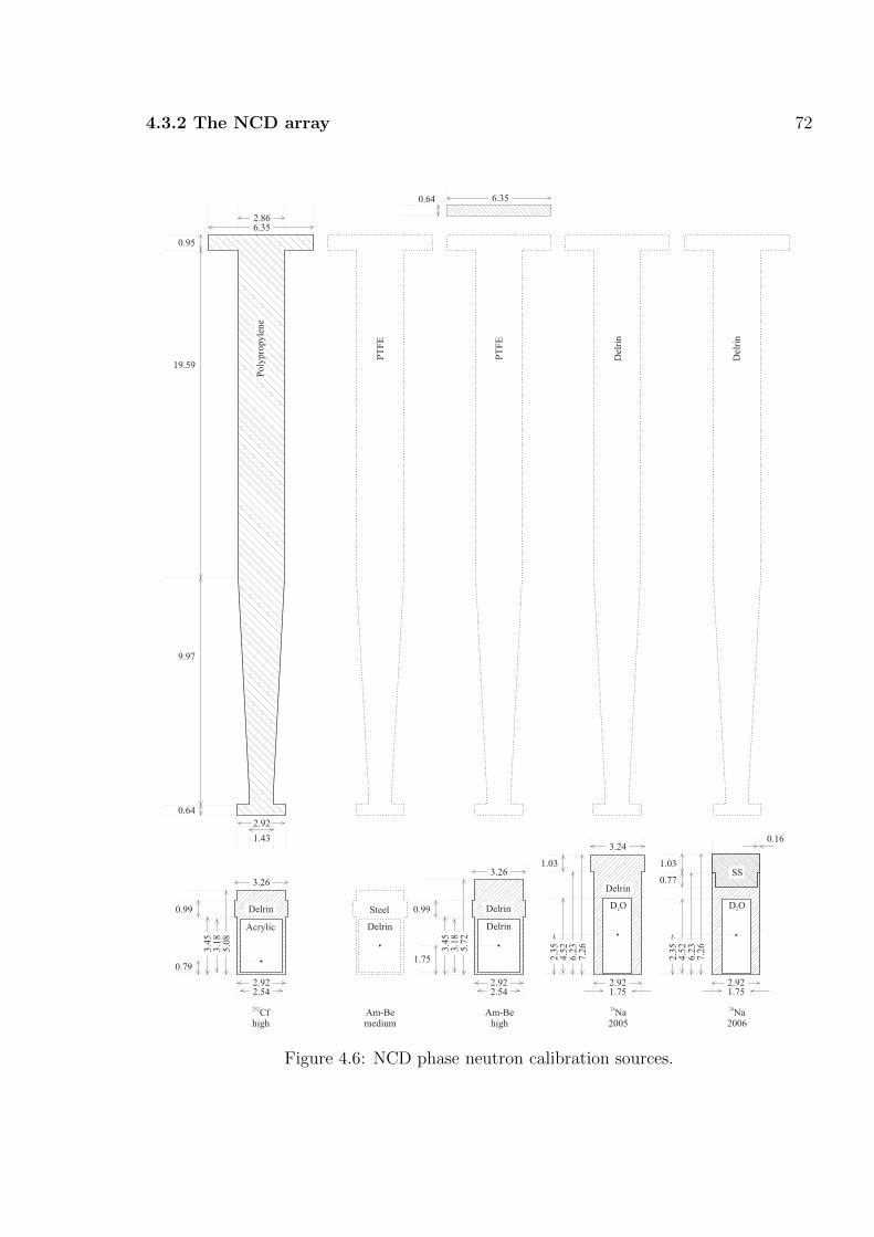
4.3.2 The NCD array 72
Figure 4.6: NCD phase neutron calibration sources.

4.3.2 The NCD array 73
z (cm)0 10 20 30 40 50 60 70 80
10
210
310
410
Figure 4.7: z-profile of source neutron captures on the materials of a source. The sourceactivity was located at z = 0.
with the spherical part of the vessel. This mass of acrylic, used to strengthen the joint,
had previously been omitted.
One omission in the geometry that remains is that of the acrylic anchor blocks to
which the NCD anchors were attached. Their effect on light propagation was studied by
Seibert [86] and found to be non-negligible; their effect on neutron propagation has not
been studied but is expected to be small as they are on the acrylic vessel.
4.3.4 Neutron calibration sources
The geometry of each neutron calibration source was composed of three parts: the source
housing, the stem and the weight/carriage apparatus, referred to as the manipulator,
to which stems were attached. The first two are shown in Figure 4.6 and the latter in
Figure 2.10. A range of different construction materials were used with different abilities
to absorb neutrons, from weakly absorbing Teflon1, used to make some of the cans, to
strongly absorbing steel, which was mainly present in the manipulator.
The author was the first to appreciate the extent of neutron re-absorption on the
materials of the sources, which could be more than 6% of all neutrons produced by a
1For a plastic, Teflon (CnF2n) is a particularly weak absorber of neutrons because it contains nohydrogen.

4.4 Calibration sources 74
source. Figure 4.7 shows the z-distribution of captures in a source run Monte Carlo
simulation where the source was located at z = 0. The bulk of the captures for this
source were on the housing (below z = 5 cm) and manipulator (above z = 34 cm); there
were relatively few captures on the Teflon stem.
The discovery of these captures helped resolve two long-standing issues in the un-
derstanding of neutron propagation in the salt phase of SNO. The first was that the
neutron mean life predicted by the diffusion equation was smaller than that measured
experimentally. After sink terms were included in the equation to approximate the effect
of absorption on the source the lifetimes agreed [87]. The second was a disagreement be-
tween different estimates for the contamination of the source neutron spectrum by prompt252Cf source gammas (see below); the result of one method was biased because it confused
gammas from neutrons capturing on the source with the prompt gammas.
The source geometries were modelled in particular detail and a database was built
to ensure that simulations for each of the calibration runs were generated with the correct
geometry. The efficacy of this database was limited by the quality of records kept by the
experiment which meant that there was sometimes uncertainty over which stem was used
in particular runs; however, the most important neutron-absorbing part of the geometry
- the manipulator - was common to all.
4.4 Calibration sources
4.4.1 Overview
This section describes the physics of the point 252Cf and AmBe neutron calibration sources
and how the source interactions are modelled in the Monte Carlo.
4.4.2 The 252Cf source
The 252Cf source produced neutrons by spontaneous fission, typically in small bursts, each
accompanied by the emission of prompt gammas and delayed neutrons from the decay
of the fission fragments. It was important to model the properties of the neutrons and
gammas in the Monte Carlo for various analyses, but particularly for testing the time
series analysis (see Appendix D) and determining the contamination of the signal window
in the in situ measurement of the 24Na source strength (see Section 6.2).
The activity in the 252Cf source was overwhelmingly due to the isotope 252Cf but

4.4 Calibration sources 75
Energy (MeV)0 1 2 3 4 5 6 7 8 9
0.00
0.02
0.04
0.06
0.08
0.10
0.12
0.14
0.16
0.18
0.20 NC
Cf 252
Figure 4.8: Energy spectra of 252Cf and NC neutrons.
there was a small contribution due to 250Cf, which produced 1.92±0.02% of the neutrons
on the source reference date of 12th June 2001 [88]. The fission of 250Cf generates an
average of 3.511 ± 0.037 neutrons per fission [89]. Its contribution to the activity was
taken into account in source strength measurements but the isotope was not modelled in
the Monte Carlo. The properties of 252Cf were modelled in some detail:
• Neutrons.
The neutron multiplicity distribution of 252Cf was described by a Gaussian of mean
3.7676 ± 0.0047 and width 1.57 [89]. The energy spectrum of the prompt neutrons
was modelled by a Maxwellian distribution with temperature 1.42 MeV (1.64×10¹⁰
K) [90]
fEdE = fP
(
dp
dE
)
dE = 2
√
E
π(kT )3exp
(
− E
kT
)
dE (4.3)
This energy spectrum is shown in Figure 4.8 where it can be compared to that of
NC neutrons.
The delayed neutrons, which were not modelled in SNOMAN, amounted to 0.0078
neutrons per fission [91]. 17 ± 5% of these had half-lives of less than 0.5 s [92].
• Gammas.
The simulation of the gammas was somewhat more involved because there is a
correlation between the total energy of the neutrons and the total energy of the

4.4 Calibration sources 76
Figure 4.9: 252Cf gamma multiplicity distributions in the Monte Carlo comparedwith experiment (left) and the energy spectrum from a 252Cf salt run simulation(right).
gammas. Nifenecker et al. [93] found the following linear relationship between the
average number of neutrons n and the average total energy of the gammas Eγ,tot
Eγ,tot = 0.75 n + 4.0 MeV (4.4)
The energy spectrum of individual gammas was described by
P (Eγ) = c√
Eγ exp
(
−Eγ
E0
)
(4.5)
which was taken from [94]. E0 = 0.62 MeV and c is a normalisation constant.
In the Monte Carlo the relationship Eq. (4.4) had to be smeared so that for given n
there was some realistic distribution of Eγ,tot(n); recall that Eq. (4.4) related an av-
erage total gamma energy Eγ,tot to an average number of neutrons n. Unfortunately
no information was available on the distribution of Eγ,tot(n), for fixed n, so the dis-
tributions had to be estimated using the gamma multiplicity distribution, which
was known from the work of Brunson [95, 96]. He found the following multiplicity
distribution, normalised to a gamma detection threshold of 140 keV
Π(G) = c1cG2 e−c2
G!+ (1 − c1)
cG3 e−c3
G!(4.6)
where G is the number of detected gammas per fission and the parameters are
c1 = 0.675, c2 = 6.78 and c3 = 9.92.

4.4 Calibration sources 77
The value of Eγ,tot from Eq. (4.4) was smeared in such a way that Brunson’s multi-
plicity distribution could be reproduced, with an artificially imposed gamma detec-
tion threshold of 140 keV. The smeared energy E ′γ,tot was given by
E ′γ,tot(n) = g(0, 2.15) + (0.75 n + 4.0) MeV (4.7)
where g(0, 2.15) is a random number sampled from a Gaussian of mean 0 and width
2.15 MeV. The width of the Gaussian was chosen to reasonably approximate the
multiplicity distribution. E ′γ,tot(n) was not allowed to drop below zero. The sim-
ulated gamma multiplicity distributions are shown, with and without smearing, in
the left hand plot of Figure 4.9. The level of agreement was more than adequate.
Tests of the simulation could be made by extracting various parameters from Monte
Carlo runs and comparing them to experimental averages compiled by Valentine
[96]. This table shows the comparison for 3 representative parameters
Quantity SNOMAN Experiment
Value Unc. Value Unc.
Mean total gamma energy 6.85 0.01 6.95 0.3Mean gamma energy 0.93 0.00 0.87 0.02Mean gamma multiplicity 8.19 0.00 7.89 0.4
The effect of the gammas on the energy spectrum measured in a 252Cf run is shown
in Figure 4.9. This distribution cannot be compared directly to SNO data because
of the large number of background events below 4 MeV.
The neutron production rate of the 252Cf source was measured using various methods that
will be discussed in Section 6.1. The resulting source strength was 16.55 ± 0.11 on 12th
June 2001. The source strength at an arbitrary time A(t) was calculated using
A(t) = A0 e−t/τ252 + f250 A0
{
e−t/τ250 − e−t/τ252}
(4.8)
where A0 = 16.55 ± 0.11 n s−1 is the activity on 12th June 2001, the 250Cf half life is
13.08 y, the 252Cf half life is 2.645 y and f250 = 0.0192 ± 0.0002 is the relative number of
neutrons produced by 250Cf as opposed to 252Cf. The error on this is given by
δA(t) = δA0 e−t/τ252 + A0 f250
√
(
δA0
A0
)2
+
(
δf250
f250
)2{
e−t/τ250 − e−t/τ252}
(4.9)
where the uncertainties on τ250 and τ252 are neglected because they are small in comparison
to the uncertainties on f250 and A0.

4.4 Calibration sources 78
4.4.3 The AmBe sources
The AmBe sources produced neutrons via (α,n) reactions. Approximately 60% of the
neutrons were accompanied by a 4.4 MeV gamma.
AmBe sources consist of the long-lived alpha-unstable isotope 241Am, which gener-
ates the alphas, and 9Be, which readily undergoes (α,n) reactions. The two most impor-
tant of the latter are9Be(α, n)12C, Q = 5.701 MeV; (4.10)
9Be(α, n)12C∗ → 12C + γ + 4.44 MeV, Q = 1.261 MeV. (4.11)
where the second is responsible for the 4.4 MeV gamma. The cross sections of the two
reactions have different dependencies on alpha energy and so their relative rates are some-
what dependent on the arrangement of the 241Am and 9Be within the source. There are
two common arrangements: in foil sources the 9Be is present as a foil next to the 241Am
and in powder sources the 9Be and 241Am are mixed together in a fine powder. One source
of each type was used in SNO during the NCD phase (the source with the higher activity
was the powder source).
This table from Croft [97] shows calculated and measured branching fractions for
the 4.4 MeV gamma-producing reaction for various different AmBe sources
Ref. Year Method B.R.
Value Unc.
[98] 1968 Calc. 0.59 0.06[99] 1970 Exp. 0.75 0.11[100] 1986 Exp. 0.558 0.031[97] 1988 Exp. 0.591 0.015[97] 1988 Calc. 0.566 0.057
There is considerable variation, reflecting the variation in internal arrangements of the
sources. Croft reported that the probability was relatively well defined only for powder
sources (he measured 0.591 ± 0.015). In the Monte Carlo this number was used for both
sources as sufficient information was not available to make an independent estimate for
the foil source. This simplification had no consequences for any of the measurements
discussed in this thesis.
The neutron energy spectra of AmBe sources are also somewhat dependent on the
individual source characteristics. The left hand plot of Figure 4.10 shows one of two

4.4 Calibration sources 79
Energy (MeV)0 2 4 6 8 10
Pro
babi
lity
0.02
0.04
0.06
0.08
0.10
0.12
0.14
0.16
0.18
37 GBq
370 GBq
Average
Figure 4.10: An experimental AmBe energy spectrum from [12] (left) and the MonteCarlo energy spectrum (right) which is the average of two measured spectra.
experimental spectra from Marsh [12]. The average of this spectrum and another, which
did not exhibit the low energy rise, was implemented in the Monte Carlo in the form a
binned PDF. The Monte Carlo spectrum is shown in the right hand plot of Figure 4.10.
As mentioned above, the energy spectrum was relatively unimportant for modelling
neutron propagation in the D2O but it did matter in the H2O. Neutron calibration sources
were deployed in the H2O close to the surface of the acrylic vessel to calibrate the detection
efficiency for neutrons produced within the acrylic of the vessel by (α,n) reactions. The
neutron capture cross section on H is highly sensitive to neutron energy, at low energies,
which made the neutron capture efficiency of the array for sources close to the acrylic
vessel also very sensitive to the neutron energy. Figure 4.11 shows the H cross section as
a function of energy and the array capture efficiency as a function of energy for a light
water AmBe run; in the latter the x-axis gives the mean energy of a Gaussian of width
1.5 MeV from which the neutron energies were sampled.

4.4 Calibration sources 80
-310
-210
-110
010
Energy (MeV)
0.0001
0.0002
0.0003
0.0004
0.0005
Cro
ss S
ection (
b)
Gaussian mean (MeV)0 1 2 3 4 5 6 7
Arr
ay c
aptu
re e
ffici
ency
0.003
0.004
0.005
0.006
0.007
0.008
0.009
0.010
0.011
0.012 / ndf 2χ 0.1831 / 2
Prob 0.9125
p0 0.001309± 0.005109
p1 0.001539± -0.001038
p2 0.0005048± 0.0005487
p3 4.862e-05± -4.792e-05
/ ndf 2χ 0.1831 / 2
Prob 0.9125
p0 0.001309± 0.005109
p1 0.001539± -0.001038
p2 0.0005048± 0.0005487
p3 4.862e-05± -4.792e-05
Figure 4.11: The energy-dependence of the neutron capture cross section on hydrogen(left) and the NCD array neutron capture efficiency as a function of neutron energy for asource placed just outside the acrylic vessel (right).

Chapter 5
Source strength measurements usinga Ge detector
I am never content until I have constructed a mechanical model of the subject
I am studying. If I succeed in making one, I understand; otherwise I do not.
WILLIAM THOMSON
Lecture notes on Molecular Dynamics and the Wave Theory of Light
This chapter presents measurements of the distributed 24Na and 222Rn neutron cali-
bration source strengths using a Ge detector. It describes the process of converting
the energy deposition spectra into source strengths. The main analysis tasks were as
follows:
• Efficiency calibration.
The efficiency of a Ge detector is the energy-dependent probability that a gamma
deposits all of its energy in the sensitive region of the detector. The efficiency can
be determined by taking measurements with calibration sources of known intensity.
However, the efficiency is a strong function of gamma energy and source geometry,
both of which differed between the calibration sources and the 24Na and 222Rn
samples. The differences were accounted for by using a Monte Carlo simulation,
tuned and verified with reference to calibration data, to predict the efficiencies.
• Dead time measurement.
Dead time fractions as high as 16% and 63% were observed in the 24Na and 222Rn
data respectively. These fractions had to be precisely quantified and corrected for.
81

Chapter 5. Source strength measurements using a Ge detector 82
• Full-energy peak integration.
The numbers of counts in the peaks in the energy deposition spectra had to be
determined consistently across all the calibration and sample data. The method
for integrating peaks had to handle a variety of background shapes and produce
numbers with statistical and systematic uncertainties.
• Detector stability measurement.
Measurements were taken over a period of almost two years and the detector stability
over than time had to be assessed.
• Implementation of the deuteron photodisintegration cross section.
Ge detectors count gammas, but the NCD array was sensitive to neutrons produced
by the gammas via photodisintegration. The cross section for this process has an
appreciable uncertainty (2%) and was an irreducible systematic in the 24Na source
strength measurement. Its value and uncertainty had to be assessed and, ideally,
other systematics controlled such that it was dominant.
All of these are discussed in the following sections. The analyses of the 24Na and 222Rn
measurements were broadly similar so, for the sake of clarity, the analysis is discussed in
detail only for the 24Na measurements. The final section describes how the 222Rn analysis
differed and presents the 222Rn results.
5.1 Ge detectors in general, and the SNO Ge detec-
tor in particular
5.1.1 Ge detectors
The semiconductor germanium can be used to build radiation detectors with excellent
energy resolution. Ge forms solid crystals in which the valence-4 Ge atoms bond covalently
with their neighbours. All valence electrons participate in covalent bonds so the valence
band is full and the conduction band is empty; the two bands are separated by an energy
gap of 0.66 eV. Energy supplied to the crystal, either thermally or through interaction
with radiation, can excite electrons into the conduction band, leaving positively charged
holes in the valence band, allowing the material to conduct.
Semiconductors are usually doped to improve their electrical properties. In a p-
type material valence-5 atoms are introduced; four electrons form covalent bonds leaving

Chapter 5. Source strength measurements using a Ge detector 83
one electron per atom loosely bound and able to move easily through the lattice. These
electrons form donor states just below the conduction band. In n-type materials, valence-
3 atoms are added producing an excess of loosely-bound holes; these form acceptor states
just above the conduction band.
If p-type and n-type materials are brought into contact in a junction the excess
electrons in the n-type material diffuse into the p-type material and combine with the
excess holes. This leaves a region around the junction, called the depletion region, across
which the remaining charged donor and acceptor states produce an electric field.
The deposition of energy in the depletion region by radiation can create electron-
hole pairs. In the electric field the electrons and holes flow in opposite directions, and,
if totally collected, the total of number electrons can form an electronic pulse with an
amplitude proportional to the energy of the radiation. A reverse bias voltage applied
to the crystal can be used to increase the size of the depletion region, and therefore the
sensitive region of the crystal, improving the charge collection efficiency.
A typical Ge detector consists of a p-type high purity Ge (HPGe) crystal partially
surrounded by a thin layer of Li, which is a dopant that is drifted into the surface of
the crystal to create an n-type layer. These layers are typically 0.1-1.5 mm thick and
are regions from which no deposited charge is collected. They are known as dead layers.
Gammas of moderate energies (hundreds of keV) pass easily into the sensitive region of
the crystal - the range of a 100 keV gamma is ∼ 4 mm - whilst the detector is shielded
from externally produced electrons and alphas, both by the dead layer and the materials
surrounding the crystal - the range of a 1 MeV electron is ∼ 1 mm and that of a 5 MeV
alpha is considerably less.
Ge detectors are favoured in the study of nuclear decays, despite the availability of
cheaper and more efficient alternatives, because of their excellent energy resolution. For
example, the typical energy resolution of a Ge detector (conventionally measured using
the 662 keV line of 137Cs) is ∼ 1 keV, while for a NaI scintillation detector it is ∼ 40 keV
[13]. The origins of the high resolution are the small amount energy required to produce
an electron hole pair (3 eV), consequent large number of events per interaction (220000
for the 662 keV gamma), and the high efficiency with which the electrons are collected.
In general the statistical contribution to resolution is actually smaller than would
naıvely be calculated using Poisson statistics. As demonstrated by Fano [101], the energy
deposited in the detector is constrained to a fixed total energy, that of the incoming
gamma, and the amount deposited in each interaction is not continuous or independent.
The correlation can act to reduce the statistical uncertainty. Fano showed that the√
N

Chapter 5. Source strength measurements using a Ge detector 84
uncertainty of Poisson statistics is modified to
δN
N=
√FN
N(5.1)
where F is the Fano factor. A typical value for a Ge detector would be 0.13 [102]. In
proportional gas counters it can be even lower but in a scintillation detector it is typically
∼ 1.
The important processes by which gammas interact with a Ge crystal are shown
schematically in Figure 5.1. At 1 MeV the dominant interaction is Compton scattering,
followed in intensity by the photoelectric (PE) effect and pair production (PP). At lower
energy the PE cross section becomes more important and the process dominates below
0.5 MeV. PP dominates above 10 MeV.
A typical Ge detector data acquisition system consists of a preamplifier, which
converts the charge pulse from the detector into a voltage pulse; a linear amplifier, to
amplify the millivolt preamp pulse into a pulse of a few volts; and a multichannel analyser
(MCA), which converts the pulse amplitude into a digital value, which can be read out
and stored.
5.1.2 Energy deposition spectra
A 24Na energy deposition spectrum is shown in Figure 5.2 to illustrate the general features
of such spectra.
24Na decays with the simultaneous emission1 of 1.369 and 2.754 MeV gammas. The
spectrum therefore has three full-energy peaks corresponding to collection of all energy
deposited by the 1.369 and 2.754 MeV gammas, and of both at once. The simultaneous
absorption of two gammas from the same cascade is known as true coincidence summing
(in contrast to random coincidence summing when the gammas are from different cas-
cades). Associated with each of these peaks are first and second escape peaks with energies
511 and 1022 keV less than the full-energy peaks. Counts appear in the first escape peak
when a PP positron, produced during absorption, annihilates and one of the 511 keV
gammas escapes. A count appears in the second when both gammas escape. Below each
full-energy peak is a Compton edge which corresponds to the maximum amount of energy
that can be transferred to an electron in a Compton scattering event. The count lies
at the edge, or below, in the Compton continuum, if the scattering gamma escapes the
1In all cascades analysed in this study the time between the emission of successive gammas is vastlysmaller than the time-resolution of the detector.

Chapter 5. Source strength measurements using a Ge detector 85
Escaping 511 keVannihilation radiation
e-
e-
e-
e-
e-
e-
e-
e-
e-
e-
e-
e-
e-
e+
e+
1
2
3
4
5
Compton scattering
Escaping scattered photon(incomplete energy loss)
e+
Figure 5.1: Processes by which a gamma can interact in a Ge detector. Event 1 contributesto the Compton continuum; events 2 and 3 lie in the full-energy peak; in event 4 a pair-produced gamma escapes and all other energy is absorbed, leaving a count in the firstescape peak; in event 5 two pair-produced gammas escape, leaving a count in the secondescape peak. Adapted from [13]

Chapter 5. Source strength measurements using a Ge detector 86
ADC bin0 1000 2000 3000 4000 5000 6000 7000 8000
10
210
310
410
510
610
1.390 MeVfull-energy peak 2.754 MeV
full-energy peak
4.144 MeVtrue-coincidentsum peak
Electronicartifact
4.144 MeVsum escape peaks
2.754 MeVescape peaks
3000 4000
1.390 MeVescape peaks
e annihilationpeak
+
2.754 MeV Compton edge
Figure 5.2: A 24Na energy deposition spectrum produced by the SNO Ge detector.
crystal without interacting further. The peak at 511 keV is believed to originate from PP
outside the Ge crystal; PP followed by annihilation of the positron produces back-to-back
511 keV gammas only one of which, because of the source-detector geometry, is likely to
be detected.
5.1.3 The SNO Ge detector
The SNO Ge detector (Princeton Gamma-Tech, Princeton, NJ; model no. IGC 5021; serial
no. 2518) contained a coaxial high purity p-type crystal mounted in a low background
cryostat (model no. NPR/12-ULB-PB). The cryostat was positioned in a cavity formed
by 2 inches of copper shielding inside 8 inches of lead shielding. The cavity was flushed
with N2 before the start of measurements to eliminate any radon and a N2 atmosphere
was maintained during data taking.
The detector electronics were configured in a standard way, described above, but
with the addition of a pile-up rejection feature in the amplifier, which, at high count rates,
decreased the time taken for the baseline to return to zero amplitude. The shaping time
constant of the amplifier was 6 µs and the MCA had 8192 channels. Data acquisition
was handled by the Maestro-32 package, version 6 (Ortec, Oak Ridge, TN). The computer
clock was set to run permanently on EDT (eastern daylight time, which is Sudbury winter

Chapter 5. Source strength measurements using a Ge detector 87
Epoxy orD O or
KCl2
7.62 cm
4.26 cm
7.77 cm
4.2
5 cm
Germaniumcrystal
Vacuum
AirGermaniumdead layer
3.53 cm0.60 cm
4.25 cm0.102 cm0.051 cm
Copper cryostatCopper can
Teflon insulator
0.102 cm
12
.78
cm
7.3
6 c
m9
.60
cm
0.1
02
cm
No
min
al 0
.1 c
m0
.10
2 c
m0
.15
0 c
m0
.07
6 c
m
0.1
5 c
m
6.91 cm7.06 cm
0.1
5 c
m
Air
Polyetheylenebeaker
Step
Lip
Figure 5.3: The Ge detector and Marinelli beaker geometry, as modelled in the MonteCarlo simulation. The actual Marinelli beakers had gently sloping sides.

Chapter 5. Source strength measurements using a Ge detector 88
ADC bin0 1000 2000 3000 4000 5000 6000 7000 8000
1
10
210
Figure 5.4: Background energy spectrum collected with an empty Marinelli beaker for 4days. The highest ADC bin corresponds to 2.826 MeV.
time).
The detector had been underground, at the SNO facility, since 1997. For most of
the time between then and these measurements it had been inactive, with the crystal
at the ambient temperature [103]. The detector was cooled down and reconditioned in
2004/05 and since then had been in continuous use. Following reconditioning, studies
demonstrated the energy linearity of the detector and measured its energy resolution to
be 1.95 keV using the 1332.5 keV line of 60Co [103]. This study is the first rigorous
efficiency calibration.
Figure 5.4 shows a background energy spectrum collected with an empty Marinelli
beaker (see below) for 4 days. Over the part of this spectrum which would contain the24Na peaks (approximately ADC bins 3000-8000) the background rate was negligible.
5.1.4 Calibration sources
This section describes the composition and geometry of the calibration sources used in
this study. The analysis of data acquired using them is left to later sections.
All sources had a Marinelli beaker geometry (see Figure 5.3), designed to maximise

Chapter 5. Source strength measurements using a Ge detector 89
the number of counts for a given sample activity2. All Marinelli beakers were manufac-
tured to the same specification and had nominal volumes of 1 litre. Some small differences
in geometry between beakers were observed - quoted volumes and fill levels could not al-
ways be completely reconciled - and in such cases the fill level was taken as the measure
of sample size when configuring the Monte Carlo.
The primary efficiency standard was a mixed radioisotope source, referred to as the
mixed source. The source (QSA Global, Germany; source no. NB 518) consisted of a
mixture of 8 radioisotopes homogeneously [104] suspended in an epoxy matrix, which
produced gammas with energies in the range 81-1836 keV. The matrix had a density
1.5 g cm−3 (see Appendix G for details of its composition). The highest energy line was
from 88Y at 2.734 MeV. The highest energy line not produced in a cascade, and therefore
subject to summing effects, was the 1115.5 MeV gamma from 88Zn.
The one sigma uncertainty on each isotope’s activity was quoted at 1.5% [20]. Com-
munication with the source manufacturer revealed that these uncertainties were not in-
dependent. The activity of each nuclide was calculated from the mass of a reference
solution added to the epoxy, whose activity was measured by the manufacturer and by
PTB (Physikalisch-Technische Bundesanstalt). Some part of the uncertainty was there-
fore correlated - relating to the amount of reference solution added to the epoxy - and
some part uncorrelated - relating to the relative amounts of each isotope in the solution.
The manufacturer could provide little quantitative guidance on how to divide up the 1.5%
uncertainty other than that it was likely to be mostly uncorrelated. The division was im-
portant as the less correlated the source strengths, the more information the calibration
provided about the efficiency of the detector. The sources strengths were conservatively
treated as being, on average, 50% correlated and 50% uncorrelated.
A high statistics mixed source run was used for the primary efficiency calibration.
Additional lower statistics runs were used to monitor detector stability.
The other sources used in this analysis were custom-made using 40K as the radioiso-
tope, supplied in the form of crystalline KCl. 40K is a naturally occurring isotope of
potassium with a half-life of 1.3× 10⁹ years [14]. It decays by electron capture producing
a 1460 keV gamma (see Figure 5.5) with probability 0.107 ± 0.002.
There were three KCl sources: the solid KCl source consisted of crystalline KCl
packed into a Marinelli beaker [103]; the first liquid KCl source was a small amount of
2Historically the use of this geometry was motivated by the small size of Ge crystals and low detectorefficiency. The disadvantage, particularly compared with a point source geometry, is the problem ofaccounting for absorption of radiation within the source. However, they remain a useful way of maximisingcount rates for low rate sources and minimising acquisition times for high rate sources.

Chapter 5. Source strength measurements using a Ge detector 90
Table 5.1: Mixed source radioisotopes [20, 14]. The reference time for the activities is Feb1st 2005 06:00:00 EDT.
Isotope Half-life (days) Gamma Ref. activity Prob. gamma
Value Unc. (keV) (kBq) Value Unc.
Ba-133 3841 7 80.997 1960 0.36680 0.00280Co-57 271.74 0.06 122.061 1780 0.85600 0.00170Co-57 271.74 0.06 136.474 1780 0.10680 0.00080Ce-139 137.64 0.02 165.860 1680 0.79900 0.00040Ba-133 3841 7 276.400 1960 0.07164 0.00020Ba-133 3841 7 302.851 1960 0.18330 0.00060Ba-133 3841 7 356.013 1960 0.62050 0.00190Ba-133 3841 7 383.848 1960 0.08940 0.00030Sr-85 64.84 0.02 514.005 7140 0.98400 0.00400Cs-137 10968 18 661.657 3910 0.85100 0.00200Mn-54 312.12 0.06 834.848 3720 0.99976 0.00000Y-88 106.62 0.01 898.042 8030 0.94400 0.00300Zn-65 243.66 0.09 1115.539 9140 0.50600 0.00220Y-88 106.62 0.01 1835.969 8030 0.99240 0.00310Y-88 106.62 0.01 2734.105 8030 0.00610 0.00020
KCl, from a different supplier, dissolved in D2O [21]; the second liquid KCl source was
a similar amount of KCl, from the same batch as the solid source, dissolved in D2O. A
summary of the different KCl sources is given in Table 5.2.
Using the KCl sources in the efficiency calibration was desirable for two reasons.
First, the 1460 keV gamma was closer in energy to the 24Na gammas than any usable line
from the mixed source, and second, the source densities were closer to the 24Na brine (and
actually identical in the case of the liquid sources). However, it was discovered during this
study (see Section 5.4) that KCl is an unsuitable material for use as a source standard,
because of the apparent unreliability of manufacturer-measured purities. But the sources
remained suitable for checking detector stability and the ability of the Monte Carlo to
predict the relative efficiencies of sources of different densities.
5.2 A Monte Carlo simulation in SNOMAN
A Monte Carlo simulation of the Ge detector allowed efficiencies appropriate for 24Na
gammas to be derived from measurements made using calibration sources with different

Chapter 5. Source strength measurements using a Ge detector 91
Table 5.2: Summary of KCl sources. Lip and step are defined in Figure 5.3. The puritiesare those specified by the manufacturers. Fill levels and masses were taken from [21, 22]
Name Material Density Fill Purity(g cm−3) (%)
Solid Crystalline KCl (1725.8 g inc. beaker) 1.24 1 mm below step 99.2Liquid 1 1170.4 g D2O + 29.975(0.027) g KCl 1.105 30.5 mm below lip 99.95(0.05)Liquid 2 1025.8 g D2O + 102.8 g KCl 1.105 Step 99.2
19K1.248 9 yEEC 1.50469
40
4-
2+
Stable
1460.851 1460
.822
18Ar40
0+
39Y106.65 dEC 3.6226
88
4-
5-
Stable
3584.7 850.
6
38Sr88
0+
2+3218.6
3-2734.130
2+1836.084
3219
.7
1382
.2
2734
.0
898.
042
1836
.063
0.065
% IEC
0.028
94.4
5.3
Figure 5.5: Decay schemes for 40K (left) and 88Y (right). Adapted from [14].
Chapter 5. Source strength measurements using a Ge detector 92
densities and producing gammas of different energies. It was the ideal way to extrapolate
in density and in energy - the physics of photon and electron transport are well understood
and there was sufficient computing power to keep statistical uncertainties small.
There is a substantial literature describing efforts to construct Monte Carlo sim-
ulations of Ge detectors (see [105] for a review), much of it describing the difficulty in
getting agreement between data and simulation. The main problems arise from the lack of
knowledge of the internal detector geometry and, to a lesser extent, the construction ma-
terials and charge-collection characteristics of the crystal (charge collection is not uniform
throughout the detector volume due to imperfections in the crystal and non-uniformity of
the electric field). This information is often not readily available, even from the manufac-
turer - Ge detectors are not mass-produced and have their own individual characteristics
and histories of use and misuse. Helmer [105] states that errors in manufacturers’ detector
position could be a few mm and that the detector axis is often not parallel to the housing
axis’.
There are two approaches to this general lack of information: the first is to measure
the internal geometry (the most efficient method uses x-rays) and the second is to fit
uncertain geometry parameters by comparison of calibration data and simulations. The
second approach was taken in this study and the parameter chosen was the dead layer, a
region of Ge surrounding the active part of the crystal, from which charge is not effectively
collected. The manufacturer could not provide a precise value (only a nominal thickness
of 1 mm) and it is a quantity with which the efficiency is strongly correlated. The aim
was to constrain the dead layer thickness using the mixed source data and use the tuned
Monte Carlo to predict efficiencies for 24Na gammas.
The Monte Carlo was constructed within the SNO Monte Carlo framework (known
as SNOMAN and described in detail in Section 4.1), which provided a geometry interfaced
with the electron and photon transport package EGS4. SNOMAN has been tested exten-
sively by the SNO collaboration and EGS4 is an industry-standard package. Adapting
SNOMAN for the Ge detector simulation involved constructing the detector and cali-
bration source geometry, adding the epoxy and KCl media, selecting appropriate EGS4
parameters and adding decay schemes and angular correlations for 24Na and 88Y. Each of
these adaptions is discussed in turn.
As much information as possible was obtained on the internal detector construction
and it was faithfully reproduced in SNOMAN: detector measurements were obtained from
communications with the manufacturer and from drawings made during repairs; the gently
sloping sides of the Marinelli beakers were approximated by vertical lines as frustums of

Chapter 5. Source strength measurements using a Ge detector 93
cones containing cavities were difficult to simulate in SNOMAN; the electronics behind
and within the crystal were neglected, as was the copper and lead shielding; and the
dead layer was assumed to have equal thickness over all surfaces of the crystal. The dead
layer on the surface facing into the well may have been smaller than the one on the outer
surface, but equal thickness was a good approximation as most gamma interactions were
with the outer layer. Likewise there were few interactions of gammas with the electronics
and shielding. Media were created for each of the sources and the density of the solid
KCl medium was scaled to account for imperfect packing of the crystals in the Marinelli
beaker.
EGS4 contains two parameters ECUT and PCUT which give the energies below which
the transport of electrons and photons, respectively, are no longer simulated; these were
set to 520 keV and 15 keV (close to the smallest possible) to maximise the quality of the
simulated energy deposition spectra (see Figure 5.6).
The decay schemes of 24Na and 88Y, two isotopes whose gammas were produced in
cascades, are shown in Figures 3.2 and 5.5. Only the 1.369 and 2.754 MeV 24Na gammas
and the 0.898, 1.836 and 2.734 MeV 88Y gammas were included in the simulation as the
branching ratios to other gammas were negligible. The 88Y branching fractions are:
Cuml. Energy (MeV)
B.R. Gamma 1 Gamma 2
0.00711 2.734 0.0000.94496 1.836 0.8981.00000 1.836 0.000
In addition to the energies and probabilities, the angular correlations between the gam-
mas had to be included as they affect the likelihood of coincident summing. Angular
correlations between two gammas can be parametrised in various ways, two common ones
being in powers of cos2 θ and in Legendre Polynomials, Pn(cos θ):
W (θ) =
l∑
i
ai cos2i θ
W (θ) =
l∑
i
aiP2i(cos θ)
where W (θ) is the probability of θ being the angle between the gammas.
The 24Na decay is a 4+−2+−0+ sequence producing two gammas which are almost

Chapter 5. Source strength measurements using a Ge detector 94
ADC bin0 1000 2000 3000 4000 5000 6000 7000 8000
1
10
210
310
410
510 Data
Tuned EGS4
Default EGS4
Figure 5.6: Simulated and experimental 24Na energy deposition spectra.
entirely E2. The coefficients can be calculated analytically [106] and the expression is
WNa(θ) = 1 +1
8cos2 θ +
1
24cos4 θ (5.2)
For the 88Y coefficients measured values [107] were used
WY (θ) = 1 − 0.1283 P2(cos θ) − 0.0243 P4(cos θ) (5.3)
5.2.1 Verification
There were a number of ways that the Monte Carlo could be verified. The three main ones
were: testing the ability of the tuned Monte Carlo to reproduce the efficiencies measured
with each of the mixed source isotopes, the relative efficiencies of the liquid and solid KCl
sources and the 24Na energy deposition spectra. The first two are discussed in Section 5.4.
Measured and simulated 24Na energy deposition spectra are shown overlaid in Fig-
ure 5.6. All features of the spectrum are reproduced in the Monte Carlo. The differences
are the magnitude of the rise in Compton back-scattering at low energies - because the
material surrounding the Ge detector was not simulated; the width of the peaks - because

Chapter 5. Source strength measurements using a Ge detector 95
the energy resolution of the Monte Carlo was perfect; and a small discrepancy at high
energies, above the 2.75 MeV peak.
A powerful quantitative test could be made by comparing relative peak areas in the24Na spectrum, which are sensitive to the modelling of detector geometry and angular
correlations. The results are shown in Figure 5.7 and there was good agreement for the
lower energy peaks, in particular. The agreement was less pleasing for the higher energy
peaks, which makes sense given the differences seen in Figure 5.6. The higher energy
peaks were not used for source strength measurements. A similar exercise was performed
using the 88Y lines in the mixed source data: 88Y has lines at 0.898 and 1.836 MeV as
well as true and random coincidence lines at 2.734 MeV (see Figure 5.5).
5.3 Full-energy peak integration
5.3.1 Determining peak areas
The shape of a typical full-energy peak can be described by the sum of three components:
• Smoothly varying background.
Contributions from the Compton continua of other lines in the spectrum, usually
described by a first or second order polynomial.
• Gaussian.
Corresponds to complete charge collection; the width comes from the statistical
variation in the number of electrons produced by a gamma of a given energy.
• Skew Gaussian and/or step function.
The are often more counts just below peaks than just above. This can occur if the
peak lies on the Compton edge of another; because Compton electrons sometimes
don’t deposit all of their energy before escaping the active region; and because of
incomplete charge collection due to crystal imperfections.
There are various ways to determine peak areas. Two common ones are fitting
the peak to a combination of the functions above (or equivalent) and estimating the
background by interpolating under the peak from regions either side of it. Peak fitting
is the most flexible and can cope with non-linear backgrounds and overlapping peaks.

Chapter 5. Source strength measurements using a Ge detector 96
Dat
a / s
imul
atio
n
0.96
0.98
1.00
1.02
1.04
1.06
1.08
Dry run Spike 1 Spike 2
Dat
a / s
imul
atio
n
0.96
0.98
1.00
1.02
1.04
1.06
1.08
Dry run Spike 1 Spike 2
Dat
a / s
imul
atio
n
0.86
0.88
0.90
0.92
0.94
0.96
0.98
1.00
1.02
1.04
050916 061127-1
Dat
a / s
imul
atio
n
0.86
0.88
0.90
0.92
0.94
0.96
0.98
1.00
1.02
1.04
050916 061127-1
Figure 5.7: Comparisons between relative peak heights in data and Monte Carlo. 24Na2.754 / 1.369 (top left), 24Na sum peak / 1.369 (top right), 88Y 1.836 / 0.898 (bottomleft), 88Y sum / 0.898 (bottom right). In the 24Na plots the comparison was made for allthree measurements and for 88Y it was made for the two highest statistics mixed sourceruns.

Chapter 5. Source strength measurements using a Ge detector 97
ADC bin4200 4220 4240 4260 4280 4300 4320 4340
310
410
510
Figure 5.8: An example 24Na peak showing the peak and background regions in the TPAinterpolation method.
Figure 5.9: An example fit peak from the mixed source data showing the step functionbackground continuum and eight Gaussians that describe the peak. The data points aregreen and the fit is black. Figure provided by Nirel [15].

Chapter 5. Source strength measurements using a Ge detector 98
Interpolation is rapid and easily applied to large amounts of data but can fail if peaks lie
on non-linear backgrounds or if they are not well separated from adjacent peaks.
A combination of both methods was applied to the data in this study. The 24Na
measurements were taken in many small runs, each consisting of large peaks on smooth
backgrounds, and were analysed using an interpolation method. Likewise the mixed source
data that were used in the analysis of detector stability. However, peaks in the primary
mixed source data were fit [23] to maximise the number that could be used.
This strategy made efficient use of calibration data and allowed consistent and rapid
analysis of the many experimental and stability spectra. It rested on the assumption that,
on average and where applicable, both methods gave the same results. The extent to which
this was the case, and the calculation of a conversion factor between the two methods, is
discussed below.
The particular interpolation method used in this study, referred to as the total peak
area (TPA) method, is described in Appendix F. An example peak on which the TPA
method was used is shown in Figure 5.8. It can be compared to a peak fit, shown in
Figure 5.9.
5.3.2 Comparison between the methods
The level of agreement between fitting and the TPA method was investigated by applying
both methods to the primary mixed source data. The results are shown in Table 5.3.
They produce very similar peak counts, except where a peak overlapped with others, or
where the background was highly non-linear.
On average the TPA method gave peak areas 0.3% larger than fitting. So a scale
factor of 0.9967 - the weighted average of the scale factors - was applied to all data
analysed with the TPA method. The standard deviation of the scale factors, 0.0058, was
converted into a general systematic uncertainty of 0.59% applied to all peak areas.
5.4 Tuning the dead layer and the KCl anomaly
5.4.1 Analysis of calibration data
For the mixed source the full-energy peak efficiency εi for gamma i was given by
εi =Ni
Si· TR
TL(5.4)

Chapter 5. Source strength measurements using a Ge detector 99
Table 5.3: Comparison between fit (from [23]) and interpolation (TPA) peak areas inthe mixed source data. In the notes column NL means the peak lay on a particularlynon-linear background and OP means that it overlapped significantly with an adjacentpeak.
Isotope Energy TPA method Fit Comparison
(keV) Counts Uncertainty (%) counts Diff. Scale Unc. Note
Stat. Sys. Tot (%)
Ba-133 81.0 1617139 0.54 1.23 1.34 1700516 -5.03 1.0516 0.0141 NLCo-57 122.1 8731522 0.12 1.01 1.02 8579800 1.75 0.9826 0.0100Co-57 136.5 1186982 0.73 2.34 2.45 1184641 0.20 0.9980 0.0245Ce-139 165.9 5465726 0.18 0.77 0.80 5177712 5.41 0.9473 0.0075 OPBa-133 276.4 1471039 0.52 0.50 0.72 1481355 -0.70 1.0070 0.0072Ba-133 302.9 3689553 0.21 0.19 0.29 3676517 0.35 0.9965 0.0028Ba-133 356.0 11412643 0.07 0.12 0.14 11354682 0.51 0.9949 0.0014Ba-133 383.8 1591569 0.41 0.36 0.55 1581508 0.63 0.9937 0.0054Sr-85 514.0 5949002 0.11 0.07 0.13 4789533 21.59 0.8051 0.0010 OPCs-137 661.7 21943586 0.03 0.08 0.08 21856992 0.40 0.9961 0.0008Mn-54 834.8 13045649 0.04 0.03 0.05 13004853 0.31 0.9969 0.0005Y-88 898.0 8837086 0.06 0.31 0.32 8752261 0.96 0.9904 0.0032Zn-65 1115.5 11663590 0.04 0.06 0.07 11628741 0.30 0.9970 0.0007Y-88 1836.0 5713957 0.05 0.03 0.06 5698784 0.27 0.9973 0.0006Y-88 2734.1 119356 0.32 0.12 0.34 118106 1.05 0.9895 0.0034

Chapter 5. Source strength measurements using a Ge detector 100
Table 5.4: Measured detection efficiencies for each of the mixed source radioisotopes [23].
Isotope Gamma Efficiency
Value Unc.
Ba-133 81.0 0.00599 0.00010Co-57 122.1 0.02458 0.00037Co-57 136.5 0.02720 0.00046Ce-139 165.9 0.02979 0.00045Ba-133 276.4 0.02671 0.00041Ba-133 302.9 0.02591 0.00040Ba-133 356.0 0.02364 0.00036Ba-133 383.8 0.02285 0.00035Sr-85 514.0 0.01929 0.00030Cs-137 661.7 0.01619 0.00025Mn-54 834.8 0.01415 0.00021Y-88 898.0 0.01249 0.00019Zn-65 1115.5 0.01174 0.00018Y-88 1836.0 0.00773 0.00012Y-88 2734.1 0.02608 0.00094
where
Si =R0iPγi
λi
(
e−λi(t0−tR) − e−λi(t1−tR))
(5.5)
is the number of gammas i produced by the source in TR, TR is the real time, TL is the
live time, Ni is the number of counts in the full-energy peak, λi is the decay constant of
the parent isotope, R0i is the activity of the parent isotope at the reference time, tR is the
reference time, Pγi is the probability of gamma emission per parent decay, t0 is the time
at the start of measurement and t1 is the time at the end of measurement.
The results from the primary calibration are shown in Figure 5.10 and Table 5.4. The
efficiency curve fitted well to
log10ε = p0 + p1E +p2
E+
p3
E 2+
p4
E 3+
p5
E 4(5.6)
which is a common efficiency curve parametrisation (see, for example, [108]).
For the KCl sources the full-energy peak efficiency was given by
ε =N
S· TR
TL(5.7)

Chapter 5. Source strength measurements using a Ge detector 101
Energy (keV)
210 310
Effi
cien
cy
-310
-210
/ ndf 2χ 2.332 / 6
Prob 0.8868
p0 0.008797± -1.957
p1 8.514e-06± -0.000126
p2 2.598± 216.2
p3 319.7± -3.608e+04
p4 3.159e+04± 2.773e+06
p5 1.858e+06± -1.138e+08
/ ndf 2χ 2.332 / 6
Prob 0.8868
p0 0.008797± -1.957
p1 8.514e-06± -0.000126
p2 2.598± 216.2
p3 319.7± -3.608e+04
p4 3.159e+04± 2.773e+06
p5 1.858e+06± -1.138e+08
Figure 5.10: Efficiency as a function of energy measured using the mixed calibrationsource. The small χ2/d.o.f. is because the efficiencies were assumed to be uncorrelatedin this fit.
where
S = msample η λ f40 Pγ ·NA
mK + mCl· (t1 − t0) (5.8)
is the number of gammas i produced by the source in TR, N is the number of counts in
full-energy peak, msample is the sample mass, η is the sample purity (by mass), λ is the40K decay constant, R0 is the 40K activity (decays per second), Pγ is the probability of
gamma emission per decay, mK is the molecular mass of K and mCl is the molecular mass
of Cl. The values of the some of these parameters are:
Parameter Value
λ (5.554 ± 0.013) × 10−10 y−1
Pγ 0.1066 ± 0.0018mK 39.098 g mole−1
mCl 35.453 g mole−1

Chapter 5. Source strength measurements using a Ge detector 102
Dead layer thickness (mm)1.00 1.05 1.10 1.15 1.20
Pre
dict
ed e
ffici
ency
0.0220
0.0222
0.0224
0.0226
0.0228
0.0230
Dead layer thickness (mm)1.00 1.05 1.10 1.15 1.20
Pre
dict
ed e
ffici
ency
0.0138
0.0139
0.0140
0.0141
0.0142
0.0143
0.0144
0.0145
0.0146
Figure 5.11: Two example Monte Carlo models for dead layer fitting: 383.8 keV 133Bapeak (left) and 834.8 keV 54Mn peak (right).
5.4.2 Tuning the dead layer
The primary mixed source calibration data were used to calibrate the Monte Carlo by
using it to fit the dead layer. When calibrated the Monte Carlo could be used to predict
the efficiencies for 24Na gammas.
The dead layer was fit by minimising the expression
χ2 =∑
i
(
ηi − εi(δ)
σi
)2
(5.9)
where the sum is over the source gammas i. εi(δ) are Monte Carlo predictions for the
efficiency as a function of dead layer thickness δ, and ηi ± σi are the measured efficien-
cies. For the fit to return the correct uncertainty on δ the uncertainties σi had to be
uncorrelated.
The models εi(δ) were obtained by running simulations for a series of dead layers
(1.0-1.2 mm for mixed source data and 1.2-1.7 mm for KCl data) and fitting second order
polynomials to the results. Two examples are shown in Figure 5.11.
As discussed in Section 5.1.4, the activities of the mixed source gammas were not
independent and so the σi were correlated. The correlations were accounted for by dividing
the uncertainty into it’s uncorrelated and correlated parts, si and ∆i respectively, related

Chapter 5. Source strength measurements using a Ge detector 103
by
σ2i = s2
i + ∆2i (5.10)
The minimisation was first performed with σi = si to give the uncorrelated uncertainty on
δ; it was then repeated with the εi(δ) shifted up and down by ∆i. The average difference
between the results was the correlated uncertainty on δ.
The mixed source fit residuals are shown in Figure 5.12. If the fit was performed
over the energy range 276.4-1115.5 keV, the best fit dead layer was 1.094 ± 0.062 mm
with a reduced χ2 of 1.54. If the fit was performed over the full-energy range 81.0-1115.5
keV, the quality deteriorated significantly - the dead layer fitted to 1.029±0.042 cm with
a reduced χ2 of 4.91. The deterioration was assumed to be due to imperfections in the
detector geometry model, which lower energy gammas, with their small mean free paths,
are more sensitive to. Higher energy gammas are more sensitive to the average geometry
rather than the detailed modelling. The energy range 276.4-1115.5 keV was selected for
this analysis because these gammas were closest in energy to the 24Na gammas, which
were the gammas the detector was being calibrated for.
These fits were repeated for the KCl sources and the results are shown in Figure 5.13.
The initial results (shown above the dashed line) were inconsistent - the same dead layer
could not reproduce the efficiencies measured using all the sources. To find the origin
of this discrepancy various investigations were undertaken into the calibration sources,
detector simulation and detector stability: mixed source data taken over an extended
period of time was analysed to demonstrate the stability of the detector; to distinguish
between a problem with the Monte Carlo or with the source strengths, calculations were
made to determine whether the relative source self-absorptions predicted by the Monte
Carlo agreed with expectations; and a second liquid KCl source was prepared, using the
KCl from the same batch as the solid source, to check whether the Monte Carlo could
predict the relative source self absorptions of two sources of different densities when the
specific source strength was the same (independent of its absolute value). The results of
these investigations are discussed in the following sections.
5.4.3 The stability of the detector
The stability of the detector was examined using both KCl and mixed source data: three
KCl runs, taken between September 2004 and July 2006, and fourteen mixed source runs,
taken between September 2005 and November 2006.
The results from the KCl source are shown in Figure 5.14. The 40K half-life is so

Chapter 5. Source strength measurements using a Ge detector 104
Energy (MeV)0.2 0.4 0.6 0.8 1.0 1.2 1.4
Res
idua
l effi
cien
cy (
data
-mod
el)
-0.0020
-0.0015
-0.0010
-0.0005
0.0000
0.0005
0.0010
0.0015
0.0020
Figure 5.12: Measured minus simulated efficiency as a function of energy using the bestfit dead layer.
Fit dead layer (mm)0.2 0.4 0.6 0.8 1.0 1.2 1.4 1.6 1.8 2.0
KCl (liquid 2)
Mixed
KCl (liquid 1)
KCl (solid)
Figure 5.13: The best fit dead layer for each calibration source. Above the dashed linethe discrepancy between the three sources is seen clearly. The agreement between thesolid and second liquid KCl source (below the line) shows the ability of the Monte Carloto extrapolate between two sources of very different density.

Chapter 5. Source strength measurements using a Ge detector 105
200401/07
200431/12
200502/07
200531/12
200602/07
Cou
nt r
ate
(Hz)
19.2
19.4
19.6
19.8
20.0
20.2
20.4
20.6
20.8
21.0 / ndf 2χ 0.3092 / 2
Prob 0.8568
p0 0.05868± 20.03
/ ndf 2χ 0.3092 / 2
Prob 0.8568
p0 0.05868± 20.03
Figure 5.14: Stability of measurements made with the solid KCl source. Uncertaintiesare statistical only.
200531/08
200531/10
200531/12
200602/03
200602/05
200602/07
200601/09
200601/11
Pea
k H
cou
nt r
ate
(Hz)
3.2
3.4
3.6
3.8
4.0
4.2
4.4
4.6
4.8
5.0 / ndf 2χ 15.9 / 13
Prob 0.2544
p0 0.02081± 3.979
/ ndf 2χ 15.9 / 13
Prob 0.2544
p0 0.02081± 3.979
200531/08
200531/10
200531/12
200602/03
200602/05
200602/07
200601/09
200601/11
Pea
k M
cou
nt r
ate
(Hz)
50
52
54
56
58
/ ndf 2χ 30.71 / 13
Prob 0.003711
p0 0.1191± 53.74
/ ndf 2χ 30.71 / 13
Prob 0.003711
p0 0.1191± 53.74
Figure 5.15: Stability of measurements made with the mixed source: 383 keV 133Ba peak(left) and 1116 65Zn peak (right). Uncertainties are statistical only.

Chapter 5. Source strength measurements using a Ge detector 106
long that no correction had to be made for depletion of the 40K in the KCl source from
one run to the next.
Representative results from two gammas in the mixed source are shown in Fig-
ure 5.15. Half-lives in the mixed source ranged from 107 to 10968 days and so rates were
corrected to an arbitrary reference time.
The KCl and mixed source time series, with uncorrelated errors only, fitted well to
straight lines. In the fit to 65Zn in the mixed source the large reduced χ2 resulted from
a single low point (possibly due to an incorrectly estimated background) and data taken
in the run for other gammas showed no such effect. In general there was no evidence for
significant variations in detector performance over time.
5.4.4 Self absorption in the calibration sources
A study was carried out to check that source self-absorptions predicted by the Monte Carlo
were consistent with expectations, based on source densities, materials and geometry. The
aim was to see whether the differences in fit dead layers could be explained by deficiencies
in the Monte Carlo. Simulations were run with 1.5 MeV gammas, an energy for which
D2O mass attenuation coefficients were available.
Mass attenuation coefficients were calculated for all source materials using a method
described in Appendix E. The mass attenuation coefficient of a material is a measure of
it’s ability to attenuate a beam of gammas; it depends on gamma energy, but is defined
in a way that makes it independent of the material density. Mass attenuation coefficients
for the calibration source materials are shown in Table 5.5 along with values of fa =
N/N0, which is the fraction of gammas that have not interacted, as a function of material
thickness. The thicknesses were meant to be representative of the path lengths traversed
by gammas in the source material. Ratios of these quantities between the sources are
given in Table 5.6.
It is reasonable to assume that the relative efficiencies of two sources were propor-
tional to their relative fa values. From Table 5.6, fa for the solid KCl source was expected
to be ∼1% lower than a liquid KCl source, compared to a Monte Carlo prediction of 1%
lower. fa for the solid KCl source was predicted to be 2.7 − 4.2% lower than the mixed
source compared to a Monte Carlo prediction of 5.5%.
These approximate calculations indicated differences between data and Monte Carlo
at the 1-2% level at most, an order of magnitude smaller than would be needed to account
for the variation in fit dead layers.

Chapter 5. Source strength measurements using a Ge detector 107
Table 5.5: Summary of net mass attenuation coefficients and fa = N/N0 values for thedifferent sources.
Source Mass attenuation coefficient Density fa = N/N0
at 1.5 MeV (cm2 g−1) (g cm−3) 1.5 cm 2.0 cm 2.5 cm
KCl + D2O 0.0516 1.105 0.9180 0.8921 0.86701.1037 0.9181 0.8923 0.8672
D2O 0.0517 1.105 0.9179 0.8920 0.8699Solid KCl 0.0504 1.240 0.9106 0.8826 0.8554Mixed 0.0536 1.500 0.8863 0.8514 0.8197
Table 5.6: Ratios of fa values between the different sources for different effective thick-nesses. The ratios are the ‘column’ source divided by the ‘row’ source.
Thickness (cm) Source KCl + D2O Solid KCl Mixed
1.5 KCl + D2O 1.000 0.992 0.965Solid KCl 1.000 0.973Mixed 1.000
2.0 KCl + D2O 1.000 0.989 0.954Solid KCl 1.000 0.965Mixed 1.000
2.5 KCl + D2O 1.000 0.987 0.945Solid KCl 1.000 0.958Mixed 1.000

Chapter 5. Source strength measurements using a Ge detector 108
5.4.5 Source strengths
The point below the dashed line in Figure 5.13 is for a second liquid KCl source, made
using KCl from the same batch as the solid source. The fit dead layer was in good
agreement with that fit using the solid source, which demonstrated the ability of the Monte
Carlo to extrapolate correctly between sources made of different materials, irrespective of
the source strength. This measurement indicated that the inconsistency of the first liquid
with the second liquid and solid KCl sources was likely to be due to errors in the source
strengths. Possible causes of source strength errors in the KCl sources were investigated.
One explanation would have been a variation in the isotopic composition from source
to source, but the 39K/40K ratio, in particular, is fixed by very fundamental processes (its
constancy is an assumption underlying the 40Ar/39Ar dating technique). Depletion of 40K
during KCl purification was considered improbable.
A more likely explanation was manufacturer error in the source purity measure-
ments. Norman et al. [109] discovered such inaccuracies in experiments searching for
differences in 40K decays rates in different chemical environments3. Using neutron ac-
tivation analysis they could determine the actual amount of potassium in their sources
and found, for example, that their ‘99.998% pure’ KCl and KNbO3 sources were only
95.3 ± 0.4% and 81.8 ± 0.3% pure respectively. It appears [110] that the manufacturers
only count ‘metallic impurities’.
Using the mixed source dead layer, Monte Carlos were run to determine the KCl
source detection efficiencies and these used to estimate the source purities:
Source MC efficiency Purity (%)
Value Unc. Value Unc.
Liquid 1 0.01077 0.00008 86.4 1.8Liquid 2 0.01077 0.00008 91.7 1.9Solid 0.01067 0.00008 92.7 1.9
The purities fit for the two sources made with KCl from the same source (solid
and second liquid) were in reasonable agreement (however, note that the errors on the
purities resulted mainly from the uncertainty in the gamma emission probability on the
decay of 40K and were therefore largely correlated). Given the doubts over the source
strengths, the KCl sources could not be used in the efficiency calibration or to cast doubt
on the efficiency calibration using the mixed source. The agreement between the two KCl
3No differences were found.

Chapter 5. Source strength measurements using a Ge detector 109
Table 5.7: Predicted 24Na efficiencies.
Peak Efficiency
Value Syst. Stat. Total
1.369 0.009946 0.000094 0.000018 0.00009582.754 0.005700 0.000058 0.000014 0.0000994Sum 0.000083 0.000002 0.000002 0.0000941
sources demonstrated the ability of the Monte Carlo to extrapolate between sources of
very different density and composition.
5.4.6 The efficiency for detecting 24Na gammas
The best fit dead layer was 1.0939 ± 0.0618 mm and Monte Carlos run using this, the24Na source geometry, and the 24Na gamma angular correlations, were used to predict the
efficiency for 24Na gammas. The results are given in Table 5.7.
5.5 Dead time
5.5.1 Understanding and modelling detector dead time
Dead times in Ge detectors can be considerable when counting high rate sources, such as
the 24Na brine. Dead time in the KCl data was less than 1% for all sources; in the mixed
source data it was 2.6-4.7%; and in the 24Na data it was in the range 0-16%. Dead time
in the 24Na and mixed source data will now be considered in turn.
If the dead time associated with an event is a constant τ , two fundamental dead
time models can be distinguished. The dead time can be non-extendable, in which case
any event occurring during τ is lost, or it can be extendable, in which case the event is
still lost but it extends the time during which the system is unable to record events by
an additional τ after it occurs.
If the dead time is non-extendable, it can be shown (see, for example, [111]), that
the recorded event rate m is related to the true event rate n by
m =n
1 + nτ(5.11)

Chapter 5. Source strength measurements using a Ge detector 110
and if the dead time is extendable they are related by
m = ne−nτ (5.12)
If the system dead time has multiple contributions from different components the rela-
tionship between m and n can be much more complicated.
The SNO Ge detector DAQ reported a live fraction for each run but the method by
which this was calculated was unknown and the fraction had no associated uncertainty.
In addition, analysis of 24Na data corrected for the reported live time gave count rates
that did not fall with the time constant expected from 24Na .
Efforts were therefore made to determine the dead time from the data itself. This
was possible because of the way the data were recorded - it was collected in a series of
runs with lengths small compared to the half-life of the decaying isotope. The change in
count rate from run to run changed the size of the dead time and allowed its magnitude
to be determined, given a model for its behaviour. Cleveland [112] demonstrated that the
detector dead time could be described by an extendable dead time model. This was done
by comparing fit qualities between the extendable and the non-extendable dead times
model applied to samples of 24Na data.
5.5.2 Dead time in the 24Na data
All 24Na data were recorded in a series of small runs, with lengths short compared to
the half-life. In each run the integral of the instantaneous count rate m(t) was recorded
between times tb and te
N =
∫ te
tb
m(t)dt (5.13)
Using Eq. (5.12) and evaluating the integral, this becomes
N =1
λτ
(
e−n0τe−λte − e−n0τe−λtb
)
(5.14)
Background was neglected because it was both constant and vastly smaller than the event
rate. The count rate at t = 0, n0, and the dead time constant, τ , could be fit by minimising
χ2 =
18∑
i=1
(
Ni − Mi
δMi
)2
(5.15)
where Mi is the number of counts recorded in run i.

Chapter 5. Source strength measurements using a Ge detector 111
Table 5.8: Dead time-corrected gamma detection rates n0 at the start of the first Gedetector run taken with each source. All times are local to Sudbury.
Data Start of counting Peak Dead time fit
set date / time n0 (s−1) Unc. τ (µs) Unc. χ2/d.o.f.
Dry run 12/09/2005 15:14:29 1.369 7.60 0.02 872.3 679.3 0.862.754 4.37 0.02 2218.0 1489.7 0.78
2005 30/09/2005 12:13:37 1.369 361.76 0.20 575.0 2.7 0.802.754 207.95 0.14 1003.8 5.5 1.77
2006 27/10/2006 14:48:17 1.369 206.64 0.18 560.9 9.5 0.982.754 118.7 0.12 1007.1 15.8 1.29
The results of fits to the dry run and both 24Na measurements are given in Table 5.8.
An example fit with residuals is shown in Figure 5.16. The fit qualities were good and
there were no trends in the residuals. The dead time constant was not well constrained by
the dry run data because the count rate, and therefore the magnitude of the dead time,
was lower than in the other two data sets.
There was one peculiarity in the fits for which no firm explanation could be found -
the extendable dead time constant τ varied as a function of energy. Its value for the 2.754
MeV 24Na peak was approximately double that for the 1.369 MeV peak, meaning that
higher energy events were less likely to be recorded. This behaviour perhaps originated
from the longer ADC digitisation time typically associated with higher energy events.
5.5.3 Dead time in the mixed source data
The simple extendable dead time model could not be successfully applied to the mixed
source data because the dead time was driven by many gammas produced with different
energies at different rates. Attempts to generalise the model were also unsuccessful. So
for the mixed source data the only option was using the dead time reported by the DAQ.
A comparison between the fit and DAQ dead times in the 24Na data could be used
to assess the accuracy of the DAQ dead time. The left hand plot of Figure 5.17 shows the
ratio of the fit dead time fraction to that reported by the DAQ for the 1.369 and 2.754
MeV peaks in the 2005 measurement. There was a 6-8% disagreement that reached its
maximum value in the limit of zero dead time.
The right hand plot shows the effect of the disagreement on the recorded number of

Chapter 5. Source strength measurements using a Ge detector 112
Hours since start of counting0 10 20 30 40 50 60 70
Cou
nts
0
500
1000
1500
2000
2500
3000
3500
4000
310×
Figure 5.16: Dead time fit and residuals for the 1.369 MeV peak in the 2005 24Na mea-surement.
Figure 5.17: The left hand plot shows the ratio of fit to DAQ dead time fractions in the2005 24Na measurement (1.369 MeV peak in red and 2.754 MeV peak in blue). The righthand plot shows the effect of the discrepancy on the recorded number of counts.

Chapter 5. Source strength measurements using a Ge detector 113
counts - i.e. the values plotted in the left hand plot weighted by the absolute magnitude
of the dead time. In the region 2.6-4.7%, which encompasses the dead time fractions
encountered in the mixed source data, the effect is negligible. Note also that the dead
time is smaller for the lower energy 24Na peak and that all mixed source gammas used
for tuning the dead layer had even lower energies.
The conclusion was that using the DAQ dead time for the mixed source data and
the fit dead time for the 24Na data would lead to accurate and consistent dead times.
5.6 The 24Na source strength
5.6.1 Probability of photodisintegration
The analysis has so far been concerned with calculating gamma production rates but
these had to be converted into neutron production rates using the photodisintegration
cross section. The conversions were done via the SNOMAN Monte Carlo so that the
interaction of gammas in materials other than D2O, such as the NCDs and AV could
be accounted for. It was of course important that the photodisintegration cross section
was properly modelled in SNOMAN. This section reviews the model and evaluates a
representative probability of photodisintegration for 24Na gammas.
The code which handles deuteron photodisintegration in SNOMAN is discussed at
length in [70]. At energies below 25 MeV the cross section was described by an analytical
model, calculated using effective range theory (ERT), multiplied by a phenomenological
function whose three parameters were fit using published experimental data. At energies
above 35 MeV a phenomenological fit due to [113] took over. In between the two, the
cross section was smoothly interpolated.
Below 20 MeV the only nuclear moments contributing significantly to the interaction
are E1 and M1. Over most of this energy range the M1 contribution is small relative to E1,
but close to threshold it becomes relatively large. An expression for σE1 can be derived
which depends only on the initial photon energy, n-p triplet effective range and physical
constants. A similar expression can be derived for σM1, depending additionally on the n-p
singlet effective range. In the derivation of the latter a significant simplification is made
- contributions due to meson exchange are neglected. No such processes occur in the E1
interaction.
The effect of neglecting meson exchange is significant. Noyes [114] estimates that
including it increases σM1 by 9.5 ± 1.2%. In SNOMAN this is assumed to be energy-

Chapter 5. Source strength measurements using a Ge detector 114
Table 5.9: Sample and reference (injected) masses. The reference mass for the dry runwas arbitrary (and only used to make comparisons between the methods) because noinjection took place.
Data set Sample mass (g) Ref. mass (g)
Value Unc. Value Unc.
Dry run 30.57 0.02 1406.2 n/a2005 30.62 0.02 968.7 0.12006 32.76 0.02 549.8 0.4
independent and the ERT σM1 is scaled up by 9.5%. The 1.2% taken as a systematic
uncertainty.
The experimental data were fit to the phenomenological model
σC = σPD
m∑
n=0
anxn (5.16)
where σC and σPD are the corrected and theoretical cross sections, and x = Eγ − E0,
where E0 is the threshold energy. The polynomial order m was fixed at 3 to give a good
fit (probability 0.25) and small difference between the theoretical and fit cross sections at
threshold (0.3%).
The statistical uncertainties on σE1 and σM1 due to input parameter uncertainties
were 0.2% and 0.1% respectively. To first order, the uncertainty on σE1 is independent
of energy. The uncertainty on σM1 was evaluated at ∼ 4 MeV for convenience and has a
weak energy dependence. To estimate the uncertainty on the phenomenological fit, Lyon
used a Monte Carlo method. For 2.2-2.7 MeV gammas he estimated an uncertainty of
0.7%.
Determining an overall uncertainty was not straightforward. The data below 5 MeV
is sparse and in his phenomenological fit, Lyon had only 4 points available, one at ∼ 5
MeV with a 7% uncertainty, and 3 at ∼ 2.75 MeV, with a combined uncertainty of 2%.
He also implicitly assumed that the theoretical cross section was correct at threshold - he
did not formally constrain the function at its lower bound, but rather used the level of
agreement as a criteria for selecting the order m, along with the goodness of fit.
The effect of different shapes for the M1 contribution was also not investigated. But
Sims [19], using the work of Chen [115], considered effective field theory (EFT) as an
alternative to ERT for calculating σE1 and σM1. She found that close to threshold EFT

Chapter 5. Source strength measurements using a Ge detector 115
Table 5.10: 24Na gamma (Rγ) and neutron (Am) production rates at the reference time(local to Sudbury). The gamma production rate is that of the sample measured by theGe detector. The neutron production rate is that of the 24Na source injected into SNO.
Data Start of counting Reference Peak Rγ (s−1) Am (n s−1)
set date / time date / time Value Unc. Value Unc.
Dry run 12/09/2005 15:14:29 12/09/2005 16:16:00 1.369 725.99 9.28 88.07 2.062.754 728.90 7.75 88.43 1.97
2005 30/09/2005 12:13:37 07/10/2005 12:37:00 1.369 14.82 0.18 1.236 0.0292.754 14.86 0.15 1.240 0.027
2006 27/10/2006 14:48:17 02/11/2006 21:20:00 1.369 20.27 0.23 0.857 0.0202.754 20.32 0.37 0.859 0.019
Table 5.11: Systematic uncertainties on the source strengths measured using the Gedetector. They were identical, within the quoted number of significant figures, in the2005 and 2006 measurements
Item Unc. (%)24Na decay constant 0.06Photodisintegration probability 1.95Ratio of sample and injected masses 0.07Full-energy peak areas 0.59Dead time fit (n0) 0.05Full-energy peak efficiency 1.09
Total 2.32

Chapter 5. Source strength measurements using a Ge detector 116
predicted a σM1 4-7% lower than ERT, and that the difference was energy-dependent.
This difference is lower than the uniform 9.5% used by Lyon. On average, the SNOMAN
cross section was found to differ from the EFT cross section by 2.2% (though this was half
the uncertainty quoted in the EFT calculations - EFT and SNOMAN did agree within
error over the energy range under study).
Overall it was felt that the model in SNOMAN was robust but that it was difficult
to use the uncertainties associated with it to constrain the uncertainty on the photodis-
integration cross section at 2.75 MeV because σC between 2.2-2.7 MeV depended on the
choice of theoretical and phenomenological models. Instead, a conservative uncertainty
was derived solely from experimental measurements at 2.75 MeV. Three measurements of
the deuteron photodisintegration cross-section at 2.75 MeV [116, 117, 118], presumably
those originally used by Lyon, were combined to yield a uncertainty of 1.9%.
From Monte Carlo simulations in SNOMAN the probability of photodisintegration
for 2.7 MeV gammas, produced uniformly in SNO, was found to be 0.002601± 0.000052,
where the uncertainty includes the 1.9% quoted above and a statistical uncertainty of
0.44%.
5.6.2 Source strengths
The gamma detection rates at the start of counting, the detection efficiency and the
photodisintegration cross section together lead directly to the source strengths.
The gamma production rate at the reference time RR was given by
Rγ =n0
εe−λ(tR−t0) (5.17)
where tR is the reference time, t0 is the start of counting, ε is the detection efficiency, and
λ is the decay constant of 24Na , 1.11208± 0.00009 days−1. The neutron production rate
Am for the activated brine injected into SNO was then given by
Am = Rγ · PPDmdist
msample(5.18)
where msample is the sample mass, mdist is the mass injected into the detector, and PPD
is the probability of photodisintegration. The sample masses are given in Table 5.9, the
results are given in Table 5.10 and a breakdown of the systematic uncertainties in ??.
The source strengths derived using the lower energy 1.369 MeV peaks were used in
the neutron detection efficiency analysis because they were closer in energy to calibration

Chapter 5. Source strength measurements using a Ge detector 117
data used to fix the dead layer. Little was to be gained from combining the results from
the two peaks given their strong correlation. The recommended source strengths are:
Data set Reference Am (n s−1)
date / time Value Unc. %
2005 07/10/2005 12:37:00 1.236 0.029 2.32006 02/11/2006 21:20:00 0.857 0.020 2.3
5.7 The 222Rn source strengths
5.7.1 Introduction
This section describes measurements of the strengths of the two distributed 222Rn sources,
which were deployed in the light and heavy water, and used to produce neutrons via pho-
todisintegration and to construct background PDFs (see Chapter 3). The measurements
and analysis were similar to those described above but there were important differences,
resulting from the gaseous nature of 222Rn and the strengths of the samples:
• All of the 222Rn prepared for injection was counted rather than just a sample.
This was to minimise the number of times the gas was transferred. The container
that was designed to hold the gas during counting could receive the gas directly
from the 222Rn generator and could be connected to the detector water systems at
injection. The vessel had fittings that allowed it to be flushed with N2 to ensure
that the efficiency of transferring the gas to the SNO detector was 100%.
• 222Rn easily diffuses through many materials.
A standard plastic Marinelli beaker was unsuitable for holding a sample during
counting and so a special metal container or can, with Marinelli-like geometry, was
constructed (shown in Figure 5.18).
• 222Rn is a gas.
There was no gaseous source available for calibrating the Monte Carlo and use had
to be made of the existing 24Na calibration. The different source self-absorptions
and geometries had to be accounted for using Monte Carlo.
• 222Rn produces no gammas directly.

Chapter 5. Source strength measurements using a Ge detector 118
Air
6.83 cm4.41 cm
6.99 cm
4.2
5 cm
4.2
5 cm
Stainless steel can
Germaniumcrystal
Vacuum
AirGermaniumdead layer
4.13 cm0.60 cm
4.25 cm0.102 cm0.051 cm
Copper cryostatCopper can
Teflon insulator
0.102 cm
Surface layer
9.8
4 c
m
10.1
6 c
m7.3
0 c
m
11.2
9 c
m
0.1
02 c
m
Nom
inal
0.1
cm
0.1
02 c
m0.1
45 c
m
0.001 cm
0.0
76 c
m
0.3
18 c
m
1.1
1 c
m
Figure 5.18: The radon can and Ge detector geometry as implemented in the Monte Carlosimulation.

Chapter 5. Source strength measurements using a Ge detector 119
222Rn alpha decays and the gammas are produced by its daughters, in particular214Bi, which is the only one that gives gammas with enough energy to photodisin-
tegrate deuterons. The decay scheme of 214Bi is complex and the energy spectra
collected during 222Rn measurements were subject to extensive random and coin-
cident summing. A Monte Carlo was used to disentangle the different spectral
contributions.
• The heavy water source was very weak and the light water source very strong.
The heavy water spike could be counted for only three hours (because of experi-
mental constraints), which exacerbated the consequences of its low source strength.
The light water source on the other hand, which was counted for five days, had an
activity in the 10s of kBq and consequently generated large detector dead times -
up to 63% - providing a stringent test of the dead time model.
The Monte Carlo was relied on more extensively in this analysis but was less well-
calibrated because of the dissimilarity between the calibration source and sample. The
measurement was less precise than 24Na but much more precise than any of the alterna-
tives [119, 120].
The following sections discuss the efficiency of the Ge detector in the new config-
uration; the method for evaluating peak areas and dead time; and the source strength
calculations.
5.7.2 The efficiency for detecting 214Bi gammas
Four lines were selected for analysis because of their strength and because they spanned
a large fraction of the energy spectrum - they were 214Bi gammas at 609, 1120, 1765 and
2204 keV.
The full-energy peak efficiencies for each of these were calculated using Monte Carlo.
Simulations were run for 214Bi only (the other main gamma-producing isotope 214Pb only
produces gammas below 0.5 MeV) using the dead layer thickness fixed in the 24Na analysis.214Bi decays were simulated either on the inner surface of the can or uniformly distributed
inside the cavity as the distribution was unknown - even though the 222Rn would have
been uniform there was concern that 214Bi and 214Pb may have plated out on the inside
surface of the can.
Systematic uncertainties were assigned to the efficiencies to account for the following
effects:

Chapter 5. Source strength measurements using a Ge detector 120
• Accuracy of the Monte Carlo 214Bi decay scheme.
This table shows a comparison of branching fractions in the Monte Carlo and pub-
lished values [121] for the lines used in this study:
Gamma Monte Literature Scale
keV Carlo Value Unc. factor
609 0.4673 0.461 0.005 0.98621120 0.1517 0.151 0.002 0.99511765 0.1622 0.154 0.002 0.94952204 0.0485 0.0508 0.0004 1.0468
Scale factors were calculated to correct the Monte Carlo-derived efficiencies and a
general uncertainty of 4.0%, equal to the standard deviation of the scale factors, was
applied to all efficiencies. The experimental uncertainties on the branching fractions
were also folded in.
• Distribution of 214Bi within the can.
As mentioned above, the distribution of 214Bi within the can was unknown and
separate simulations were run for the two extreme scenarios - with 214Bi on the
inner surface and distributed throughout the cavity. For each line the average value
was taken as the central value and the difference between the two as a systematic
uncertainty. The size of the uncertainty varied from 4.4% for the lowest energy peak
to 0.2% for the highest energy peak.
• Uncertainty in the dead layer thickness.
Monte Carlos were run with the best fit dead layer of 1.094 mm and the upper and
lower bounds of 1.040 mm and 1.156 mm. The difference in efficiencies, ranging
between 0.5% and 3.0%, was taken as a systematic uncertainty.
Other effects were more difficult to quantify, in particular the consequences of the
change in detector geometry. It was not clear that it was justifiable to use the dead layer
derived in the 24Na analysis in simulations using the radon can. If, for example, the
gamma ray attenuation in the plastic of the Marinelli beaker was modelled incorrectly
then the dead layer thickness would have been tuned to compensate - while not a problem
in the 24Na analysis, this might give misleading results when the plastic was replaced by
another material. It had to be assumed that the process of fitting the dead layer was
tuning only that part of the geometry, internal to the Ge detector, that was common

Chapter 5. Source strength measurements using a Ge detector 121
ADC bin0 1000 2000 3000 4000 5000 6000 7000 8000
1
10
210Bi
0.609
214
Bi1.120
214 Bi1.765
214
Bi2.204
214
Pb0.352
214
Figure 5.19: A measured radon spectrum with select gammas from 214Pb and 214Bi la-belled.
Energy (MeV)
0.0 0.5 1.0 1.5 2.0 2.5 3.0
1
10
210
310
410
510
Bi0.609
214
Bi1.120
214
Bi1.765
214
Bi2.204
214
Figure 5.20: A Monte Carlo radon spectrum. Simulations runs with decays of the radondaughter 214Bi only.

Chapter 5. Source strength measurements using a Ge detector 122
between the 24Na and radon geometries. This hypothesis was supported by the good
agreement as a function of energy seen in Figure 5.12.
Example experimental and Monte Carlo energy deposition spectra are shown in
Figures 5.19 and 5.20. Notable differences between the two are the omission of low energy
gammas and lines due to 214Pb in the Monte Carlo. The efficiencies calculated using the
Monte Carlo are given in Table 5.12.

Chapte
r5.
Sourc
estre
ngth
measu
rem
ents
usin
ga
Ge
dete
cto
r123
Table 5.12: Monte Carlo efficiencies from 214Bi simulations. The systematics are MC (accuracy of Monte Carlo decay scheme),BF (experimental uncertainties on branching fractions), 214Bi (distribution of activity within the can) and D. layer (uncertaintyon the dead layer thickness).
Gamma Surface eff. Cavity eff. Systematics (fractional) Corrected efficiency
(keV) Value Unc. Value Unc. MC BF 214Bi D. layer Value Stat. Syst.
609 0.008705 0.000033 0.008993 0.000033 0.0403 0.0108 0.0326 0.0052 0.008726 0.000016 0.0004651120 0.001858 0.000015 0.001911 0.000015 0.0403 0.0132 0.0283 0.0181 0.001875 0.000008 0.0001011765 0.001628 0.000014 0.001646 0.000014 0.0403 0.0130 0.0110 0.0106 0.001554 0.000007 0.0000692204 0.000416 0.000007 0.000426 0.000007 0.0403 0.0079 0.0235 0.0298 0.000440 0.000004 0.000025
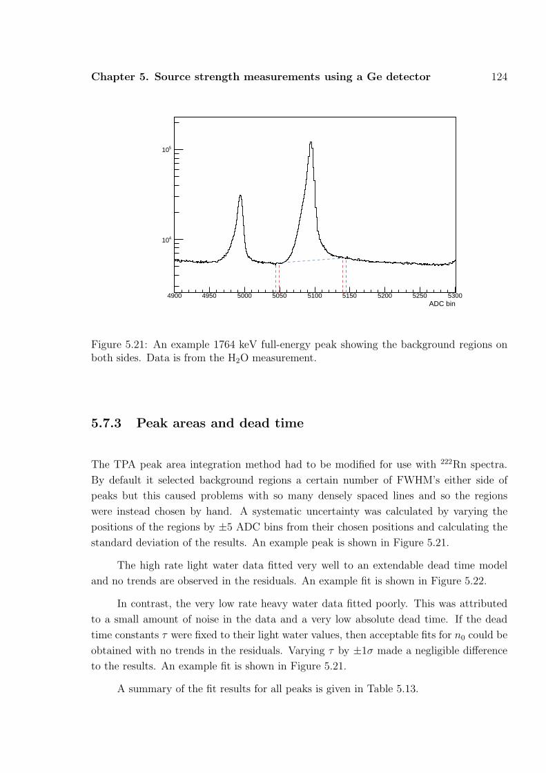
Chapter 5. Source strength measurements using a Ge detector 124
ADC bin4900 4950 5000 5050 5100 5150 5200 5250 5300
410
510
Figure 5.21: An example 1764 keV full-energy peak showing the background regions onboth sides. Data is from the H2O measurement.
5.7.3 Peak areas and dead time
The TPA peak area integration method had to be modified for use with 222Rn spectra.
By default it selected background regions a certain number of FWHM’s either side of
peaks but this caused problems with so many densely spaced lines and so the regions
were instead chosen by hand. A systematic uncertainty was calculated by varying the
positions of the regions by ±5 ADC bins from their chosen positions and calculating the
standard deviation of the results. An example peak is shown in Figure 5.21.
The high rate light water data fitted very well to an extendable dead time model
and no trends are observed in the residuals. An example fit is shown in Figure 5.22.
In contrast, the very low rate heavy water data fitted poorly. This was attributed
to a small amount of noise in the data and a very low absolute dead time. If the dead
time constants τ were fixed to their light water values, then acceptable fits for n0 could be
obtained with no trends in the residuals. Varying τ by ±1σ made a negligible difference
to the results. An example fit is shown in Figure 5.21.
A summary of the fit results for all peaks is given in Table 5.13.

Chapter 5. Source strength measurements using a Ge detector 125
Table 5.13: Summary of dead time fit results.
Data set Gamma n0 (s−1) τ (µs) χ2 / d.o.f. Count rate (Bq)
(keV) Value Unc. Value Unc. Value Unc.
D2O 609 1.538 0.021 936.06 Fixed 2.08 175.82 10.161120 0.343 0.011 4312.05 Fixed 0.56 180.96 10.471765 0.313 0.007 4711.60 Fixed 1.05 198.95 11.572204 0.082 0.004 18235.50 Fixed 0.88 193.60 15.33
Ave. 184.90 9.10
H2O 609 1089.35 0.94 936.06 0.41 0.90 124515 69831120 245.20 0.59 4312.05 4.82 0.85 129512 62531765 210.05 0.46 4711.60 5.95 1.01 133604 70832204 57.49 0.26 18235.50 52.96 0.50 135152 8946
Ave. 130135 6145
Table 5.14: Parameters used in the 222Rn source strength analysis. All times Sudburylocal times. The Ge detector computer runs on winter time all year round and D2O startof counting time has been corrected by one hour.
Parameter Value
Half-life of 222Rn (days) 3.8235 ± 0.0004D2O start of Ge counting 11/08/2006 06:20:32D2O reference time 11/08/2006 10:40:00H2O start of Ge counting 03/11/2006 15:14:04H2O reference time 08/11/2006 20:21:00

Chapter 5. Source strength measurements using a Ge detector 126
5.7.4 Source strengths
This section describes how the four source strengths derived for each radon measurement
- one for each gamma - were combined. Unlike 24Na there was no good reason to prefer a
source strength derived with any particular gamma. For each measurement the strengths
were combined taking into account the correlations between them.
The uncertainties due to the modelling of the gamma cascade were taken to be
random and the all others to be 100% correlated; numerically this corresponded to an
almost equal division of the uncertainties into correlated and uncorrelated parts. The
source strengths, with their uncorrelated errors, were combined in the standard way (see
Appendix B). The reduced χ2 for the heavy water measurement was 1.91 and so the final
error was inflated accordingly; the reduced χ2 for the light water spike was 0.79 so the
error was not changed. The procedure was then repeated with the central values shifted up
and down by the correlated parts of their uncertainties, with the largest change in central
value for each measurement symmetrized to give the combined correlated uncertainty.
Correlated and uncorrelated uncertainties were then added in quadrature.
The final activities, in 222Rn decays per second, were:
Data set Reference Activity (Bq)
date / time Value Unc. %
D2O 11/08/2006 10:40:00 180.4 9.2 5.1H2O 08/11/2006 20:21:00 50700 2100 4.1

Chapter 5. Source strength measurements using a Ge detector 127
Hours since start of counting0.0 0.5 1.0 1.5 2.0 2.5 3.0 3.5
Cou
nts
50
60
70
80
90
100
110
120
130
140
150
Hours since start of counting0 20 40 60 80 100 120
Cou
nts
270
280
290
300
310
320
330
340
350
310×
Figure 5.22: Dead time fit and residuals for the 1764 keV peak in the D2O data (top) andfor the 2204 keV peak in the H2O data (bottom).

Chapter 6
Source strength measurements usingthe PMT array
Never express yourself more clearly that you are able to think.
NEILS BOHR
This chapter describes measurements of the strengths of the 252Cf , 24Na and AmBe
neutron calibration sources. The 252Cf source was calibrated absolutely and served
as the standard reference source in the NCD phase. Its strength was measured using three
separate methods, which are described in the first section. The 24Na and AmBe sources
were calibrated relative to the 252Cf source using the SNO detector. In this in situ method
they were positioned at the centre of the detector and the PMT neutron detection rates
compared to those recorded with the 252Cf source in the same position. The calibration
of the 24Na and AmBe sources is discussed in the second and third sections, respectively.
6.1 The 252Cf source strength
6.1.1 Measurements
A physical description of the 252Cf source can be found in Section 4.4.2. This section
describes the measurement of its activity, defined as the number of neutrons produced
per second at the site of the activity within the source housing (as distinct from the
number of neutrons exiting the source housing). Three methods were used:
128
6.1 The 252Cf source strength 129
• D2O multiplicity.
In this technique [122, 123] the neutron multiplicity distribution measured during
the D2O phase was fit to an analytical model. The model gave the probability that
in one unit of time - the data were divided into 2 second units - d neutrons would
be detected from r produced in N 252Cf fissions; it could be written
P (d) =
∞∑
N=1
∞∑
r=d
r!εdεr−d
d!(r − d)!· e−
(r−Nµ)2
2Nσ2
2Nπσ2· λNe−λ
N !(6.1)
where λ is the 252Cf fission rate, µ is the mean of the multiplicity distribution, σ is
the width of the multiplicity distribution and ε is the neutron detection efficiency.
The D2O data were used because of the relative ease with which neutron events could
be identified by cuts on event position and energy. In the salt phase the neutron
diffusion length was much smaller so it became difficult to distinguish neutron events
from high energy prompt gammas.
The neutron detection efficiency ε was corrected for the sacrifice of the cuts used to
identify neutrons to give a source strength of 16.33 ± 0.18 n s−1.
• Time series.
The time series analysis (see Appendix D), like the method described above, also
harnessed the bursty nature of the 252Cf source, but in a more complete and general
way. It allowed five parameters to be fit independently: the source strength, neutron
detection efficiency, neutron mean lifetime and the contamination of the neutron
signal by prompt fission gammas and radioactive backgrounds. The inclusion of the
prompt fission gammas meant that the method could be used in the salt phase. The
source strength was found to be 16.46 ± 0.12 n s−1.
• Direct counting.
In the direct counting method [88] an array of 3He proportional counters was used
to directly measure the 252Cf neutron production rate. The experimental arrange-
ment (shown in Figure 6.1) consisted of three rings of 3He proportional counters,
supported by a polyethylene moderator, and surrounding a well where the sources
were placed. There were 42 counters in all but only the inner 24 were used. The
neutron detection efficiency of the array was evaluated using two methods:
1. In the fission-triggered evaluation a sample of the same 252Cf used to make the
source was electroplated onto a Si(Li) surface barrier detector and covered by
a further barrier detector. The detectors acted as fission triggers which opened

6.1 The 252Cf source strength 130
8.89 cm16.51 cm24.13 cm
AirAir
Polyethylene
Steel wall
He3
Acrylicsource
Polyethyleneblock
5.08 cm27.94 cm
z = 0
27
.94
cm
15
.00
cm
10.16 cm
35
.56
cm
2.54 cm
= 0q
Figure 6.1: The 3He proportional counter apparatus used in the direct countingmeasurement of the 252Cf source strength. Section (left) and plan (right).
a 200 µs window for observing 252Cf neutrons in the array. (This was assumed
to contain the majority of the prompt neutrons but source strengths measured
using this window were corrected to a long 1000 µs window to include the
remaining prompt and delayed neutrons). The measured multiplicity distribu-
tion was fit to a model to determine the fission rate and therefore the array
efficiency, which was found to be εft = 0.2668 ± 0.0023.
2. In the Pt disk evaluation 252Cf was electroplated onto two platinum disks. The
deposited activities were measured using a Frisch grid chamber before the disks
were placed separately in the well and the event rates measured. The efficiency
was found to be εPt = 0.2755 ± 0.0020, which is the weighted average of the
values found using each disk: 0.2733 ± 0.0027 and 0.2792 ± 0.0029.
The 252Cf source was placed in the array and the measured count rate converted into
a source strength using each of the efficiencies. The source strength was initially
found to be 17.78± 0.16 using the fission triggered efficiency and 17.22± 0.14 using
the Pt disk efficiency. The weighted average of these was 17.45 ± 0.30 n s−1
There were a few issues with this analysis that the author investigated. The first
was the 2.2% (1.2σ) discrepancy between the two Pt disk measurements; the second
was the 3.3% (2σ) discrepancy between the εft and εPt measurements; and the third
was the discrepancy between the direct counting and the multiplicity and time series

6.1 The 252Cf source strength 131
measurements, which agreed well with each other.
One possible explanation for the first two was inconsistent positioning of sources
inside the well. For the last, a possibility was moderation and absorption of neutrons
by the acrylic in which the 252Cf was encapsulated. A Monte Carlo simulation of the
apparatus was built within the SNOMAN framework to help quantify the magnitude
of these effects. The plots in Figure 6.2 show the results.
The top two figures show the dependence of the 200 and 1000 µs array efficiencies on
the vertical position of the source in the well. The Monte Carlo efficiencies at z = 0
were within ∼ 3% of the measured values, which was reassuring, particularly as no
attempt was made to simulate the response of the counters - capture efficiencies
were equated to detection efficiencies. This level of agreement was sufficient in a
study of relative effects.
The 200 µs efficiency increased with increasing z because neutrons produced further
up in the well were less likely to enter the mass of polyethylene below the well,
where they were well moderated but less likely to reach a counter in 200 µs. The
behaviour of the 1000 µs efficiency resulted from two competing effects: a tendency
of the efficiency to fall with an increase in position because neutrons became less
well moderated and therefore less likely to capture, and a tendency of it to rise
because neutrons were produced closer to the centre of the array and were more
likely to reach counters. The decrease won at smaller displacement and the increase
at larger displacements.
If inconsistencies in the mounting of the Pt disks in the well caused differences in
vertical position of 0.5 cm then the discrepancy between the values for the two discs
would fall below 1σ. The difference between εft and εPt measurements could not be
explained by any vertical displacement consistent with the experimental procedure.
The effect of the source housing was investigated by running simulations with and
without the 252Cf source encapsulated in acrylic. The hypothesis was that the
acrylic surrounding the source might moderate the neutrons and thereby increase
the efficiency of the array compared to what it would have been for the bare activity.
The bottom right plot of Figure 6.2 shows the efficiency correction factor as a
function of the position of the Pt disk/triggered source, when the acrylic source was
placed at the bottom of the well (where its activity would be located at the centre
of the acrylic housing, at z = 1.28 cm). Assuming the Pt disk/triggered source was
at z = 0, the correction was found to be 2.25 ± 0.08%. This result was confirmed
by Hime [124] who found a correction of 2.15 ± 0.20% using an independent code.
The correction was responsible for removing most of the discrepancy between the

6.2 The 24Na source strengths 132
Table 6.1: Results of the methods for determining the 252Cf source strength. The referencedate is June 12, 2001.
Method Strength (n s−1)
Value Unc.
D2O multiplicity 16.33 0.18Salt time series 16.46 0.12Frisch grid 16.75 0.14Triggered Si(Li) 17.08 0.43
Weighted mean 16.55 0.11
direct counting and other methods.
Hime refined other aspects of the analysis [124] and the final source strengths were
17.08 ± 0.43 (fission triggered) and 16.75 ± 0.14 (Pt disks).
The source strengths from all methods are summarised in Table 6.1. They were combined
using the standard method (see Appendix B); the error was scaled up by 1.37 to account
for a slightly large χ2 of 5.2.
6.2 The 24Na source strengths
6.2.1 Overview
This section describes the calculation of the distributed 24Na source strengths using a
cross-calibration technique, which related the strength of the injected 24Na to the strength
of the 252Cf source.
In each 24Na measurement a sample of the activated brine was encapsulated in a
small can (see Figure 4.6), which was attached to the source-manipulator system and
positioned in the centre of the SNO detector. The neutron detection rate was measured
in this configuration and then with the 252Cf source in the same position. As the 252Cf
source strength was known the 24Na source strength could be inferred. The analysis
could be done using either the PMT or NCD array to detect the neutrons. The author
was responsible for the PMT analysis.
If RNa is the dead time-corrected neutron detection rate measured using the canned

6.2 The 24Na source strengths 133
z (cm)∆0.0 0.5 1.0 1.5 2.0 2.5 3.0 3.5 4.0 4.5 5.0
s)µIn
ner
coun
ter
capt
ure
effic
ienc
y (<
200
27.5
27.6
27.7
27.8
27.9
28.0
28.1
28.2
28.3
28.4
28.5 / ndf 2χ 12.78 / 18
Prob 0.8043
p0 0.0305± 27.78 p1 0.02974± 0.1076
p2 0.005872± -0.005602
/ ndf 2χ 12.78 / 18Prob 0.8043
p0 0.0305± 27.78 p1 0.02974± 0.1076
p2 0.005872± -0.005602
z (cm)∆0.0 0.5 1.0 1.5 2.0 2.5 3.0 3.5 4.0 4.5 5.0
s)µIn
ner
coun
ter
capt
ure
effic
ienc
y (<
1000
32.5
32.6
32.7
32.8
32.9
33.0
33.1
33.2
33.3
33.4
33.5 / ndf 2χ 11.64 / 18
Prob 0.8651
p0 0.03299± 32.99 p1 0.03216± -0.1026
p2 0.006351± 0.01716
/ ndf 2χ 11.64 / 18Prob 0.8651
p0 0.03299± 32.99 p1 0.03216± -0.1026
p2 0.006351± 0.01716
z (cm)∆0.0 0.5 1.0 1.5 2.0 2.5 3.0 3.5 4.0 4.5 5.0
Cor
rect
ion
(%)
16.0
16.5
17.0
17.5
18.0
18.5
19.0
19.5 / ndf 2χ 22.98 / 18
Prob 0.1914p0 0.0511± 18.75 p1 0.0491± -0.8214 p2 0.00959± 0.0855
/ ndf 2χ 22.98 / 18Prob 0.1914p0 0.0511± 18.75 p1 0.0491± -0.8214 p2 0.00959± 0.0855
z (cm)∆0.0 0.5 1.0 1.5 2.0 2.5 3.0 3.5 4.0 4.5 5.0
Cor
rect
ion
(%)
1.0
1.5
2.0
2.5
3.0
3.5
4.0 / ndf 2χ 11.41 / 17
Prob 0.8344p0 0.1325± 2.186 p1 0.232± 0.3838 p2 0.1166± -0.08893 p3 0.01616± 0.005006
/ ndf 2χ 11.41 / 17
Prob 0.8344p0 0.1325± 2.186 p1 0.232± 0.3838 p2 0.1166± -0.08893 p3 0.01616± 0.005006
Figure 6.2: The 200 µs array capture efficiency (top left), 1000 µs capture efficiency (topright), 200-1000 µs correction factor (bottom left) and the correction to the efficiencymeasured with an unencapsulated source to make it applicable for the acrylic 252Cf source(bottom right). All plots show the variation of the quantity as a function of the distanceof the production point above the bottom of the well. Points are fit to polynomials toillustrate the general dependence - there is no physical motivation for the functional forms.The efficiencies in the top two plots are percentages.

6.2 The 24Na source strengths 134
24Na source and RCf is the dead-time corrected corresponding to the production of 1 n s−1
by the 252Cf source, both scaled to some reference time, then the strength of the 24Na
injected into SNO Am is given by
Am =1
fCfP
RNa
RCf
mm
mNa(6.2)
where mm is the mass of the injected brine, mNa is the mass of brine in the can and fC
and fP are two correction factors, discussed below.
The correction factor fC accounted for the different detection efficiencies of 252Cf
and 24Na neutrons. The efficiencies differed because the former were produced within the
source but the latter were generated by photodisintegration in a cloud extending some
distance from the source (the radiation length of 2.754 MeV gammas was ∼ 26 cm). The
efficiencies were related by
εNa = fC εCf
where
fC =εNa
MC
εCfMC
(6.3)
was calculated using Monte Carlo.
The correction factor fP accounted for the different photodisintegration probabili-
ties of gammas produced by the canned and distributed 24Na sources. Gammas from the
canned source could interact with the materials of the can, which reduced the photodis-
integration probability compared to gammas from the distributed source. The photodis-
integration probabilities were related by
Am = fPmm
mNa
ANa
where
fP =P m(PD)
P Na(PD)(6.4)
The quantities P m(PD) and P Na(PD) are photodisintegration probabilities for the dis-
tributed and canned sources, respectively, calculated using Monte Carlo.
The Monte Carlo simulations used to calculate these correction factors are described
in the following section along with the measurement of the ratio RNa/RCf . However, first
is a discussion of the cuts used to identify neutrons events.

6.2 The 24Na source strengths 135
Table 6.2: Analysis cuts. Parameters are described in the text.
Cut
DAMN0 & 0xCCF56FE1^0x0400000
0.55 < ITR < 1.00−1.0 < u · r < 1.0−0.12 < β14 < 0.95
5.5 < ERSP < 10 MeV200 < r < 450 cm
6.2.2 Data selection
Cuts were developed to distinguish events in the PMT array due to neutrons from those
due to backgrounds and instrumentals. They fell into two categories: ‘standard’ SNO
analysis cuts to remove instrumental, muon and other events; and analysis-specific cuts
to distinguish neutrons from gammas produced by the sources and by U and Th in the
materials of the detector. The cuts are listed in Table 6.2. The analysis-specific cuts are
shown below the line.
The analysis cuts are standard ones on u.r, which is the projection of the direction
vector on the radius vector; β14, which is a measure of the isotropy of PMT hits in the
event; and ITR, which is the fraction of the detected photons falling in the prompt peak.
These cuts were designed to remove non-physics events or events for which the position
fitter returned non-sensical results. β14 and ITR are discussed further in Section 8.2.4.
The DAMN mask is a specification of which low level instrumental cuts should be applied;
the mask used in this analysis was identical to the one used in the analysis of neutrino
data except that it excluded the burst cut. This cut could not be used with a bursty
fission source.
The analysis-specific cuts were on event energy and position. Figure 6.3 shows
measured energy-radius distributions for canned 24Na and 252Cf runs. These are the
classes of event that compose the distributions:
• Neutrons.
Neutrons mainly captured on deuterons producing 6.25 MeV gammas. The events
were concentrated at low radii, close to the source, but the distribution had an
exponential tail out to high radii.

6.2 The 24Na source strengths 136
• Sources gammas.
In the 24Na sources these were 1.37 and 2.54 MeV gammas from the decay of 24Mg∗,
the beta decay final nucleus, and in the 252Cf source they were gammas from the
de-excitation of the fission fragments. These gammas could be reconstructed some
distance from the source location because of two effects: first, a gamma could travel
some distance before Compton scattering an electron (and thereby producing the
Cerenkov signal that was detected) and second, the finite position resolution of the
detector. Monte Carlo-generated distributions for 24Na and 252Cf source gammas
are shown in the top plots of Figure 6.4.
• Low energy U and Th backgrounds.
Gammas from the U and Th decay chains (see Appendix A) were a background at
low energies and particularly at high radii, close to the relatively low-radiopurity
AV and H2O. The energy-radius distribution for a neutrino run, where the majority
of the events are U and Th gammas, is shown in the lower plot of Figure 6.4.
• Miscellaneous.
A number of minor processes could generate neutrons indistinguishable from those
produced directly by the sources. Neutrons produced by (α, n) reactions in the
acrylic of the AV, NC neutrino interactions and photodisintegration by U and Th
gammas had low enough rates to be neglected. Those produced by photodisintegra-
tion by source gammas were included in the Monte Carlo.
The analysis region was selected to maximise the neutron rate and exclude background
events; it lay within 200 < r < 450 cm and 5.5 < T < 10 MeV.
6.2.3 Radial neutron production profile (fC)
The correction factor fC accounted for the different neutron detection efficiencies of 252Cf
and 24Na neutrons, resulting from the different radial neutron production profiles. It was
defined in Eqn. 6.3
fC =εNa
MC
εCfMC
To calculate εNaMC it was important that the radial production profile (shown in
Figure 6.5) be correct in the Monte Carlo. To test this the 2.754 MeV gamma radiation
length was extracted from a simulation and compared to a calculation. The Monte Carlo
distribution fitted to a decaying exponential with radiation length 25.80 ± 0.38 cm. A

6.2 The 24Na source strengths 137
1
10
210
RSP energy (MeV)
0 2 4 6 8 10 12 14 16 18 20
Rad
ius
(cm
)
0
100
200
300
400
500
600
700
800
1
10
210
310
410
RSP energy (MeV)
0 2 4 6 8 10 12 14 16 18 20
Rad
ius
(cm
)
0
100
200
300
400
500
600
700
800
Figure 6.3: Measured energy-radius distributions for 252Cf (left) and 24Na (right). Thebox highlights the analysis region. These plots are intended to illustrate the relativedistributions of events in energy-radius space; there happens to be more events in the24Na plot but this is of no consequence.
theoretical value was calculated using D2O mass attenuation coefficients prepared by
[125]. These were extrapolated to 2.754 MeV to give a coefficient of 0.0422 cm2 g−1,
which corresponded to a radiation length of 26.19 ± 0.52 using a D2O density of 1.1056
g cm−3. There was therefore good agreement between Monte Carlo and calculation.
The right hand plot of Figure 6.5 shows the simulated radial capture distributions
for 252Cf and 24Na . The 252Cf distribution is higher than Na at low radii, the distributions
cross at about 100 cm, and 24Na neutrons are preferentially detected at higher radii. The
steep rise at low radii in both distributions is a volume effect.
Values of fC were calculated using reconstructed Monte Carlo, that is, using Monte
Carlo fit in the same way as the data to take into account any biases or artifacts in
the position and energy reconstruction algorithms. For diagnostic purposes values were
calculated as a function of radial bin and lower radial cut.
Figure 6.6 shows fC by radial bin and as a function of lower radial cut. The Monte
Carlo used was the sum of that produced for the dry run and the 2005 spike. The
correction factors for the second spike were derived separately using dedicated Monte
Carlo.
The task of predicting fC was actually a demanding one for the Monte Carlo because
it relied on proper modelling of the propagation of neutrons and gammas over distances

6.2 The 24Na source strengths 138
1
10
210
RSP energy (MeV)
0 2 4 6 8 10 12 14 16 18 20
Rad
ius
(cm
)
0
100
200
300
400
500
600
700
800
1
10
210
RSP energy (MeV)
0 2 4 6 8 10 12 14 16 18 20
Rad
ius
(cm
)
0
100
200
300
400
500
600
700
800
1
10
210
RSP energy (MeV)
0 2 4 6 8 10 12 14 16 18 20
Rad
ius
(cm
)
0
100
200
300
400
500
600
700
800
Figure 6.4: Energy-radius distributions for three PMT backgrounds: Monte Carlo sim-ulation of 252Cf gammas (top left), 24Na gammas (top right) and (mainly) low energybackground events from a neutrino run (bottom). The box highlights the analysis region.

6.2 The 24Na source strengths 139
Figure 6.5: Radial neutron production profile of 24Na photodisintegration neutrons (left)and radial capture profiles (right) of 24Na neutrons (red) and 252Cf neutrons (blue). They-axis units are arbitrary. The plots show the actual positions of the verticies in theMonte Carlo rather than ones reconstructed using position fitters.
Radius (cm)100 150 200 250 300 350 400 450
Cor
rect
ion
fact
or
0.8
0.9
1.0
1.1
1.2
1.3
1.4
1.5
Radius (cm)100 150 200 250 300 350 400 450
Cor
rect
ion
fact
or
0.8
0.9
1.0
1.1
1.2
1.3
1.4
1.5
Figure 6.6: Correction factor fC by radial bin (left) and as a function of lower radial cut(right). The error bars give the statistical uncertainties and the green bands give thesystematic uncertainties.
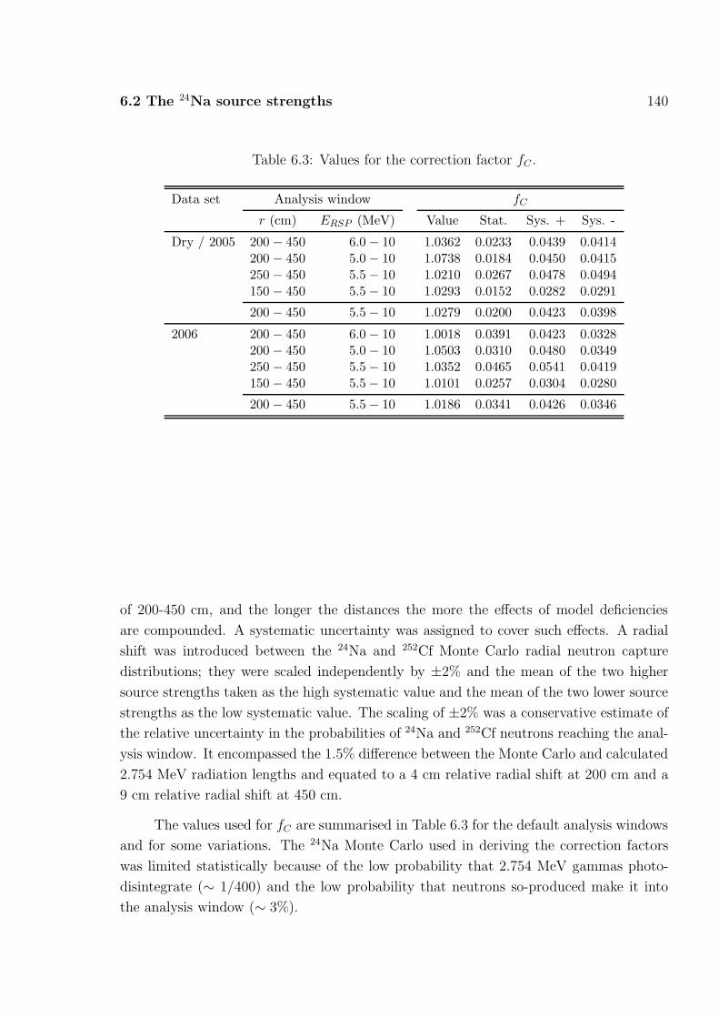
6.2 The 24Na source strengths 140
Table 6.3: Values for the correction factor fC .
Data set Analysis window fC
r (cm) ERSP (MeV) Value Stat. Sys. + Sys. -
Dry / 2005 200 − 450 6.0 − 10 1.0362 0.0233 0.0439 0.0414200 − 450 5.0 − 10 1.0738 0.0184 0.0450 0.0415250 − 450 5.5 − 10 1.0210 0.0267 0.0478 0.0494150 − 450 5.5 − 10 1.0293 0.0152 0.0282 0.0291
200 − 450 5.5 − 10 1.0279 0.0200 0.0423 0.0398
2006 200 − 450 6.0 − 10 1.0018 0.0391 0.0423 0.0328200 − 450 5.0 − 10 1.0503 0.0310 0.0480 0.0349250 − 450 5.5 − 10 1.0352 0.0465 0.0541 0.0419150 − 450 5.5 − 10 1.0101 0.0257 0.0304 0.0280
200 − 450 5.5 − 10 1.0186 0.0341 0.0426 0.0346
of 200-450 cm, and the longer the distances the more the effects of model deficiencies
are compounded. A systematic uncertainty was assigned to cover such effects. A radial
shift was introduced between the 24Na and 252Cf Monte Carlo radial neutron capture
distributions; they were scaled independently by ±2% and the mean of the two higher
source strengths taken as the high systematic value and the mean of the two lower source
strengths as the low systematic value. The scaling of ±2% was a conservative estimate of
the relative uncertainty in the probabilities of 24Na and 252Cf neutrons reaching the anal-
ysis window. It encompassed the 1.5% difference between the Monte Carlo and calculated
2.754 MeV radiation lengths and equated to a 4 cm relative radial shift at 200 cm and a
9 cm relative radial shift at 450 cm.
The values used for fC are summarised in Table 6.3 for the default analysis windows
and for some variations. The 24Na Monte Carlo used in deriving the correction factors
was limited statistically because of the low probability that 2.754 MeV gammas photo-
disintegrate (∼ 1/400) and the low probability that neutrons so-produced make it into
the analysis window (∼ 3%).

6.2 The 24Na source strengths 141
6.2.4 Probability of photodisintegration (fP)
The correction factor fP accounted for the different deuteron photodisintegration proba-
bilities for gammas from canned and distributed 24Na . It was defined in Eqn. 6.4
fP =P m(PD)
P Na(PD)
Gammas produced by the former could be absorbed or scattered by the material of the
can before they had a chance to photodisintegrate and the probability of them doing so
was therefore smaller. The can dimensions and materials are shown in Figure 4.6; in the
first measurement the can was made entirely of Delrin but in the second it was fitted with
a stainless steel lid.
Values for the probabilities of photodisintegration (PD) were taken from Monte
Carlo simulations:
Type P(PD) 1/P(PD)
Value Unc. Value Unc.
Distributed 0.002596 0.000009 385.27 1.32Can (2005) 0.002564 0.000007 389.97 1.03Can (2006) 0.002523 0.000009 396.38 1.39
The probability was lower for the 2006 measurement because of the steel lid, which at-
tenuated the gammas more strongly.
The main focus of this section is the uncertainty on fP due to P(PD). Delrin was
added to the SNOMAN Monte Carlo specifically to allow fP to be calculated and it was
important to check that interactions of gammas with Delrin were handled correctly. Infor-
mation was available to do this - Evans [126, 127] performed an experiment to measure the
mass attenuation coefficient of Delrin at 2.754 MeV. SNOMAN was used to simulate the
experimental configuration and assign a systematic uncertainty on P(PD), and therefore
on fP , based on the ability of the Monte Carlo to reproduce the result of the experiment.
The mass attenuation coefficient µ/ρ (see Appendix E) is a parameter well-characterising
the interactions of gammas with a material.
In the experiment a small quantity of activated 24Na brine was enclosed in a thin-
walled vial and positioned a short distance from the face of a Ge detector. The 1.369
and 2.754 MeV full-energy peak counts R were measured with and without a Delrin disk
placed between the source and the detector. The quantity A, given by
A =Rwith
Rwithout= e−(µ/ρ)xρ (6.5)

6.2 The 24Na source strengths 142
Figure 6.7: Delrin mass attenuation coefficient experimental configuration, as simulatedin SNOMAN.
was calculated for each peak, corrected for the change in source strength between mea-
surements and used to infer the mass attenuation coefficient. The measured values and
mass attenuation coefficients were:
Gamma A µ/ρ (cm2g−1)
(keV) Value Unc. Value Unc.
1369 0.9497 0.0014 0.0562 0.00162754 0.9631 0.0022 0.0410 0.0025
where the uncertainties are statistical only.
These coefficients can be compared to calculated values. Taking the chemical com-
position of Delrin to be (CH2O)n [128] and using elemental mass attenuation coefficients
from [129], the mass attenuation coefficients of Delrin were found to be 0.0572 at 1.369
MeV and 0.0398 g cm−2 at 2.754 MeV, which were in good agreement with the measured
values.
The important features of the experimental setup were reproduced in the Monte
Carlo. The geometry is shown in Figure 6.7. In constructing it several simplifications
were made:

6.2 The 24Na source strengths 143
• Materials.
The Ge detector had no outer casing and the crystal had no dead layer. No attempt
was made to simulate the charge collection characteristics of the detector. The vial
materials were neglected. No attempt was made to simulate materials surrounding
the apparatus from which photons might scatter back into the detector. These
simplifications were minor because the measurement was a relative one, concerned
only with the change in count rate when the disk was placed in front of the detector.
• Disk thickness.
The thickness of the Delrin disk differed slightly from the experiment to reflect the
difference in densities - 1.4 g cm−3 in SNOMAN compared to 1.434(0.007) g cm−3
in the experiment. The thickness was adjusted to give the same mass per unit area
of 0.9177 g cm−2.
The EGS4 photon and electron cut offs (see Section 5.2) were set to PCUT = 0.025
and ECUT = 0.526 to add detail to the energy deposition spectra. Following the exper-
imental procedure, events were classed as falling in full-energy peaks if the deposited
energy was within 0.5 keV either side of the nominal gamma energy.
This table shows the Monte Carlo-derived mass attenuation coefficients µsim/ρ along
with the experimental and calculated values (uncertainties are statistical):
Gamma Asim µsim/ρ (g cm−2) µexp/ρ (g cm−2) µcalc/ρ (g cm−2)
(keV) Value Unc. Value Unc. Value Unc. Value Unc.
1367 0.9518 0.0030 0.0538 0.0034 0.0562 0.0016 0.0572 n/a2754 0.9662 0.0045 0.0375 0.0051 0.0410 0.0025 0.0398 n/a
All results were consistent, but it was decided to take convert the difference between the
simulated and experimental central values into a systematic uncertainty. A difference
in mass attenuation coefficients would imply an uncertainty in the probability of gam-
mas scattering from the source material and, because scattered and unscattered gammas
have different energy distributions and the photodisintegration cross section is energy-
dependent, this would imply an uncertainty in the photodisintegration probability.
The probability of a 2.754 MeV gamma causing a photodisintegration P (PD) could
be written
P (PD) = P (PD | s) · P (s) + P (PD |ns) · P (ns)
= P (PD | s) · P (s) + P (PD |ns) · (1 − P (s))
= P (s) · [P (PD | s) − P (PD |ns)] + P (PD |ns) (6.6)

6.2 The 24Na source strengths 144
Energy (MeV)
0.0 0.5 1.0 1.5 2.0 2.5 3.0
410
510
Energy (MeV)
2.2 2.3 2.4 2.5 2.6 2.7 2.8 2.9 3.0
)2
Cro
ss-s
ectio
n (c
m
-2810
-2710
-2610
-2510
-2410
-2310totσ
PDσ
Figure 6.8: Energy distribution of 2.754 MeV gammas after a single Compton Scattering(left); D2O total and photodisintegration cross sections (right).
where P (s) is the probability of scattering and P (ns) = 1−P (s) is the probability of not
scattering. An uncertainty due to the difference in mass attenuation coefficients would
create an uncertainty δP (s) on P (s). The resultant uncertainty on P (PD) was
δP (PD)
P (PD)=
P (PD | s) − P (PD |ns)
[P (PD | s) − P (PD |ns)] · P (s) + P (PD |ns)· δP (s) (6.7)
To evaluate this, the quantities P (s), δP (s), P (PD | s) and P (PD |ns) had to be calcu-
lated.
P (s) was calculated using µexp/ρ and an estimate of 0.6 cm for the characteristic
thickness of material gammas passed though before entering the D2O. The uncertainty
δP (s) was the change in P (s) when µexp/ρ was replaced by µsim/ρ. The calculated value
was P (s) = 0.033 ± 0.003.
P (PD |ns) could be found simply, but P (PD | s) required a knowledge of the energy
distribution after scattering as well as the photodisintegration cross section.
To calculate the energy distribution after scattering, the intensity as a function of
angle was first found using the Klein-Nishina formula [130]
I(θ)
I(θ = 0)=
1
[1 + γ(1 − cos θ)]2·(
1 + cos2 θ +γ2(1 − cos θ)2
1 + γ(1 − cos θ)
)
(6.8)
where γ = Eγ/mec2 and θ is the angle through which the gamma was scattered. An-

6.2 The 24Na source strengths 145
Table 6.4: Values for the correction factor fP taken from Monte Carlo.
Data set fP
Value Stat. Sys.
Dry run / 2005 1.0122 0.0044 0.0019
2006 1.0288 0.0050 0.0019
gles were sampled randomly from this distribution and converted to energies using the
standard Compton formula
E ′(θ) =Eγ
1 + γ(1 − cos θ)(6.9)
The resulting energy distribution is shown in Figure 6.8. The probability of twice-
scattered gammas photodisintegrating was neglected; any such events would have reduced
the systematic uncertainty and neglecting them made the value of the systematic conser-
vative.
P (PD | s) was given by
P (PD | s) =
∫
σPD(E)
σtot(E)dE (6.10)
where the integral is over the energy distributions. σPD was taken from [70] and σtot calcu-
lated using D2O mass attenuation coefficients from [125]1. It was found that P (PD | s) =
0.00041. Using Eqn. 6.10 with E = 2.754 MeV gave P (PD |ns) = 0.00122. And substi-
tuting both of these into Eqn. 6.7 gave δP (PD)P (PD)
= 0.0019, which was the final systematic
uncertainty. The values of fP are summarised in Table 6.4.
6.2.5 Source strengths
The 252Cf data were used to determine RCf , which was the count rate within analysis
cuts that corresponded to the production of 1 n s−1. For each 24Na run the count rate at
the start of the run RNa was calculated from the number of counts within the analysis
cuts N using
RNa =Nλ
1 − e−λL(6.11)
1µ/ρ = σtot/m where µ/ρ is the mass attenuation coefficient and m is the atomic/molecular mass.

6.2 The 24Na source strengths 146
Figure 6.9: Fits to the radioactive decay law, with the 24Na half life fixed, yieldingactivities at the start of the first run in each data set. Dry run (top), 2005 (middle) and2006 (bottom).

6.2 The 24Na source strengths 147
Radius (cm)50 100 150 200 250 300 350 400 450
)-1
Ref
eren
ce s
ourc
e st
reng
th (
ns
0.5
1.0
1.5
2.0
2.5
Uncorrected
Corrected
Radius (cm)50 100 150 200 250 300 350 400 450
)-1
Ref
eren
ce s
ourc
e st
reng
th (
ns
0.5
1.0
1.5
2.0
2.5
Uncorrected
Corrected
Nominal cut
Radius (cm)50 100 150 200 250 300 350 400 450
)-1
Ref
eren
ce s
ourc
e st
reng
th (
ns
0.4
0.6
0.8
1.0
1.2
1.4
1.6
1.8
Uncorrected
Corrected
Radius (cm)50 100 150 200 250 300 350 400 450
)-1
Ref
eren
ce s
ourc
e st
reng
th (
ns
0.4
0.6
0.8
1.0
1.2
1.4
1.6
1.8
Uncorrected
Corrected
Nominal cut
Figure 6.10: Raw and corrected source strengths by bin (left) and as a function of lowerradial cut (right) for the 2005 measurement (top) and 2006 measurement (bottom). Errorbars are statistical.
Table 6.5: Reference masses and times. The reference (injected) mass for the dry run isarbitrary as no injection took place.
Data set Sample mass (g) Ref. mass (g) Reference date / time
Value Unc. Value Unc.
Dry run 10.92 0.02 1406.2 0.0 Sep 12th 2005 16:16:00 EDT2005 10.36 0.02 968.7 0.1 Oct 7th 2005 12:37:00 EDT2006 10.80 0.02 549.8 0.4 Nov 2nd 2006 21:20:00 EST

6.2 The 24Na source strengths 148
Table 6.6: Mixed source strengths (Am) in n s−1. The last value in the section for eachdata set corresponds to the default analysis cuts.
Data set Analysis window Raw Corrected source strength (Am)
r (cm) ERSP (MeV) Value Unc. Value Sys. + Sys. - Stat.
Dry run 200 − 450 6.0 − 10 83.46 3.39 81.53 3.50 3.30 3.78200 − 450 5.0 − 10 87.94 2.69 82.90 3.52 3.25 2.91250 − 450 5.5 − 10 83.81 3.89 83.08 3.93 4.06 4.42150 − 450 5.5 − 10 86.30 2.26 84.86 2.40 2.47 2.55
200 − 450 5.5 − 10 84.37 2.93 83.08 3.47 3.27 3.30
2005 200 − 450 6.0 − 10 1.301 0.040 1.271 0.055 0.051 0.048200 − 450 5.0 − 10 1.364 0.032 1.286 0.055 0.050 0.037250 − 450 5.5 − 10 1.304 0.046 1.293 0.061 0.063 0.057150 − 450 5.5 − 10 1.296 0.026 1.275 0.036 0.037 0.032
200 − 450 5.5 − 10 1.304 0.034 1.284 0.054 0.050 0.042
2006 200 − 450 6.0 − 10 0.804 0.018 0.824 0.038 0.028 0.028200 − 450 5.0 − 10 0.841 0.015 0.810 0.034 0.028 0.031250 − 450 5.5 − 10 0.821 0.022 0.816 0.043 0.034 0.042150 − 450 5.5 − 10 0.801 0.012 0.816 0.025 0.023 0.024
200 − 450 5.5 − 10 0.802 0.016 0.810 0.034 0.028 0.031
Table 6.7: Contributions to the uncertainties on the 24Na source strengths measured usingthe PMT array.
Item Unc. (%)
2005 2006
Correction factor fP 0.47 0.52Correction factor fC (statistical) 1.95 3.35Correction factor fC (radial scaling)) 3.99 3.79Ratio of sample and injected masses 0.19 0.20

6.2 The 24Na source strengths 149
where λ is the 24Na decay constant and L is the run length. These were converted into
source strengths by dividing by RCf .
The sets of source strengths for each measurement (dry run, 2005 or 2006) were
fitted to the radioactive decay law with the 24Na half-life fixed to find the strength at
the start of the first run (see Figure 6.9). These were scaled to the reference times and
masses, and the Monte Carlo corrections applied, using Eq. (6.2).
Corrected and uncorrected source strengths are shown in Figure 6.10 for each of the
data sets, by radial bin and as a function of lower radial cut. The analysis was done in a
single large radial bin so plots with many radial bins are for illustration only. The correc-
tion factors were successful in accounting for most of the strong radial dependence of the
uncorrected source strengths. Final source strengths for different radial and energy cuts
are shown in Table 6.6. Contributions to the final uncertainties are shown in Table 6.7.
6.3 The AmBe source strengths
6.3.1 Overview
This section describes the calculation of the strengths of the AmBe sources using a cross-
calibration method similar to that outlined above. A physical description of the two
AmBe sources used in the NCD phase can be found in Section 4.4.3.
Pairs of AmBe and 252Cf runs were identified that were taken close to the centre of
the detector at similar times. They were distributed relatively uniformly over the periods
of time when each source was in use - the medium rate source was used mainly towards
the beginning of the NCD phase and the high rate source towards the end. For each pair,
the PMT neutron detection rates RAmBe and RCf were measured and the AmBe source
strength AAmBe was calculated using
AAmBe =RAmBe
RCfACf (6.12)
where ACf is the activity of the 252Cf source. Detection rates were corrected for dead time,
which was non-negligible, particularly for the high rate AmBe runs. The same analysis
window was used as before; AmBe gammas are somewhat higher in energy than those
from 252Cf and 24Na but not enough to affect the choice of cuts.
For each of the sources a straight line was fit to the time series of source strengths,
with only the statistical (uncorrelated) errors included on each point. If the reduced χ2

6.2 The 24Na source strengths 150
was greater than 1 then the fit uncertainty was scaled up by√
χ2/d.o.f. to compensate
(see Appendix B). Figure 6.11 shows the results run-by-run, which were consistent over
time.
Each of the fit source strengths was then scaled by a correction factor fC , which
accounted for the different detection efficiencies of AmBe and 252Cf neutrons. These
differed because the sources produced different numbers of photodisintegration neutrons
and because different amounts of neutrons captured back on the source materials. fC was
defined by
εAmBe = fC εCf
where
fC =εAmBe
MC
εCfMC
(6.13)
such that
< AAmBe >corrected=< AAmBe >
fC
(6.14)
where < AAmBe > is the fitted source strength. fC was assumed to be the same for all
source pairs, with the same rate AmBe source, and was calculated by summing together
Monte Carlo for the relevant AmBe runs and using a single very high statistics 252Cf
simulation. fC was 1.015 ± 0.007 for the medium rate source and 1.012 ± 0.007 for the
high rate source.
The uncertainties on the 252Cf source strength and the correction factor fC were
combined in quadrature with the scaled fit uncertainty.
6.3.2 Source strengths
The final source strengths were 23.63±0.27 Hz for the medium rate source and 68.70±0.74
Hz for the high rate source. The uncertainties were split almost equally between statistics
and the 252Cf source strength uncertainty.
Figure 6.12 shows the dependence of the source strengths on radius. The lack of a
strong dependence on radius across the analysis region gives confidence in the modelling
of neutron propagation in the Monte Carlo and indicated an absence of contamination,
which would be unlikely to be uniform in radius. No explanation has been found for the
slight turn down in the highest radius bin, which was also seen in the 24Na analysis; the
bin carried little weight because the number of events was small.

6.2 The 24Na source strengths 151
Run number
48000 49000 50000 51000 52000 53000 54000 55000 56000
Sou
rce
stre
ngth
(H
z)
22.0
22.5
23.0
23.5
24.0
24.5
25.0
25.5
26.0 / ndf 2χ 4.868 / 8
Prob 0.7716p0 0.1834± 23.99
/ ndf 2χ 4.868 / 8Prob 0.7716p0 0.1834± 23.99
/ ndf 2χ 4.868 / 8Prob 0.7716p0 0.1834± 23.99
/ ndf 2χ 4.868 / 8Prob 0.7716p0 0.1834± 23.99
Run number
54000 56000 58000 60000 62000 64000 66000 68000
Sou
rce
stre
ngth
(H
z)
62
64
66
68
70
72
74
76 / ndf 2χ 30.56 / 18
Prob 0.03233p0 0.3441± 69.47
/ ndf 2χ 30.56 / 18Prob 0.03233p0 0.3441± 69.47
/ ndf 2χ 30.56 / 18Prob 0.03233p0 0.3441± 69.47
/ ndf 2χ 30.56 / 18Prob 0.03233p0 0.3441± 69.47
Source strength (Hz)21.0 21.5 22.0 22.5 23.0 23.5 24.0 24.5 25.0 25.5 26.00.0
0.5
1.0
1.5
2.0
2.5
3.0
Source strength (Hz)62 64 66 68 70 72 74 760
1
2
3
4
5
Figure 6.11: Source strengths as a function of run number (top) projected onto the y-axes (bottom). Medium rate source (left) and high rate source (right). Uncertainties arestatistical only.

6.2 The 24Na source strengths 152
Radius (cm)100 200 300 400 500 600
Sou
rce
stre
ngth
(H
z)
19
20
21
22
23
24
25
26
27
28 / ndf 2χ 0.6778 / 3
Prob 0.8784p0 0.2431± 23.58
/ ndf 2χ 0.6778 / 3Prob 0.8784p0 0.2431± 23.58
/ ndf 2χ 0.6778 / 3Prob 0.8784p0 0.2431± 23.58
/ ndf 2χ 0.6778 / 3Prob 0.8784p0 0.2431± 23.58
Radius (cm)100 200 300 400 500 600
Sou
rce
stre
ngth
(H
z)
62
64
66
68
70
72
74 / ndf 2χ 0.9546 / 3
Prob 0.8122p0 0.6018± 68.54
/ ndf 2χ 0.9546 / 3Prob 0.8122p0 0.6018± 68.54
/ ndf 2χ 0.9546 / 3Prob 0.8122p0 0.6018± 68.54
/ ndf 2χ 0.9546 / 3Prob 0.8122p0 0.6018± 68.54
Figure 6.12: Source strengths as a function of radial bin. Medium rate source (left) andhigh rate source (right). Uncertainties are statistical only and the central values havebeen corrected with fC .
6.4 Summary
In the chapter measurements of the strengths (neutron production rates) of the two 24Na
sources and the two AmBe sources used in the NCD phase have been reported. They are
summarised in the table below, with errors symmetrised. Reference dates are given for the24Na sources as 24Na has a half-life which is not long on the timescale of the experiment.
Source Data set Reference Source strength (n s−1)
date / time Value Unc. %24Na 2005 7/10/2005 12:37:00 1.284 0.067 5.224Na 2006 2/11/2006 21:20:00 0.810 0.044 5.4
AmBe med 23.63 0.27 1.1AmBe high 68.70 0.74 1.1

Chapter 7
The Neutron Detection EfficiencyUsing Point Sources
But there are also unknown unknowns - the ones we don’t know we don’t know.
A member of the US administration.
(2002)
The goal of this analysis was to make a theoretical prediction of the NCD NC neutron
detection efficiency - the probability that an NC neutron produced in the heavy
water was detected by the NCD array.
The prediction was made using a Monte Carlo simulation of the detector, tuned using
AmBe point source neutron calibration data. The tunable parameter was the hydrogen
concentration in the heavy water, referred to as the hydrogen fraction, on which there was
a significant experimental uncertainty. The performance of the tuned Monte Carlo was
evaluated by making comparisons between data and simulations with a larger set of point
source data than were used for the tuning. The systematic uncertainty on the prediction
of the detection efficiency was evaluated by propagating uncertainties on the Monte Carlo
input parameters, including those relating to the isotopic composition of the heavy water
and the detector geometry. This approach complemented the 24Na measurement in a
number of ways:
• It was independent.
The point source method used a different set of calibration data and was therefore
largely independent. The two methods acted as powerful checks of each other.
153

Chapter 7. The Neutron Detection Efficiency Using Point Sources 154
• It did not depend on the strength of a calibration source.
It was not limited by the precision with which the strength of any particular cali-
bration source was known; it relied instead on the high precision of MCNP and a
detailed model of the detector geometry. As a theoretical number, it was limited
only by the completeness of the model and the uncertainties on its input parame-
ters. Point source data was used to tune the Monte Carlo in a relative way, such
that source strengths cancelled.
The absolute point source strengths were used only when testing the ability of the
tuned Monte Carlo to reproduce the measured efficiencies. These tests were of the
consistency of the data with the tuned Monte Carlo and no uncertainty was applied
based on the ability to make the comparison (the degree of knowledge of the source
strengths is one part of this uncertainty).
• It had different systematics.
It did not suffer from the dominant systematic in the 24Na measurement associated
with the ability to demonstrate the uniformity of the source. There was an analogue,
associated with the knowledge of the positions of the point sources used to tune the
Monte Carlo, but it was more easily dealt with.
The first section of this chapter describes the point source data taken during the NCD
phase and how it was analysed; the second section covers the tuning of the hydrogen
fraction; the third evaluates the performance of the tuned Monte Carlo by making com-
parisons with calibration data; and the fourth describes the evaluation of NC efficiency
and its systematic uncertainties. A final section describes the measurement of efficiencies
for NC neutrons in the PMT array and for photodisintegration neutrons in the PMT and
NCD arrays.
7.1 Point source data
7.1.1 Overview
This section describes the point source data taken during the NCD phase and how it was
analysed for this study. The aim was to form a data set that was suitable for use in fitting
the hydrogen fraction and for making comparisons between data and Monte Carlo. A set
of source positions were identified and, for each of these, a representative average efficiency
was evaluated, which could be compared with average simulated efficiencies generated for
the same points.

Chapter 7. The Neutron Detection Efficiency Using Point Sources 155
Figure 7.1: Source positions in one of the vertical planes (red dots) in a full AmBe scan[16].
7.1.2 The point source data
Point source calibration data was taken with AmBe and 252Cf neutron sources. Most
runs were taken with the AmBe sources because they were of much higher rate. This
maximised statistics and reduced the amount of lost neutrino live time associated with
neutron calibrations.
The sources could be positioned at various points on two perpendicular planes inter-
secting on the z-axis of the detector (see Figure 2.10). The manipulator system could not
reach positions on the diagonals because the ropes would have become entangled with the
array. Some runs at large absolute x and y had to be very long to ensure that a significant
number of neutrons reached the counters of the inaccessible strings on the diagonals.
Sets of measurements taken with the AmBe sources, referred to as scans, were
acquired on approximately a monthly basis; they were either mini scans, for which the
source positions were selected to ensure that each string received a large number of counts,
or full scans, which had larger numbers of source positions such that all counters received
a large number of counts. The source positions in one plane for a full scan are shown in
Figure 7.1.
Around 5% of the NCD phase detector live time was devoted to collecting AmBe
neutron calibration data. Such a large amount of data was necessary so that significant

Chapter 7. The Neutron Detection Efficiency Using Point Sources 156
numbers of neutron events could be collected on each of the 156 counters on a regular
basis. The data was used in a variety of studies on the neutron detection efficiency and
response of the counters to neutron events.
252Cf data were taken less frequently and in a smaller subset of positions, typically
at, or towards, the centre of the array, though there was one comprehensive scan along
the central z-axis of the detector. The 252Cf runs were mainly used by the time series
analysis (see Appendix D).
7.1.3 Run selection
A subset of 103 AmBe runs were selected for this analysis out of the several hundred
taken during 13 scans in the NCD phase. The run selection criteria were:
• AmBe runs only.
Only runs taken with the medium and high rate AmBe sources were selected. The252Cf data were lower rate, deployed less frequently and its burstiness generated
dead time behaviour in the NCDs that was difficult to model.
The strengths of the two AmBe sources were determined in Section 6.3. The domi-
nant contribution to the strength of each source was that of the 252Cf source, which
they were calibrated with reference to. The uncertainties on the strengths of the
two AmBe sources are therefore largely correlated and so, in this analysis, nothing
was to be gained by treating them as distinct sources.
• Good spatial and temporal coverage.
A set of source positions was identified that provided good spatial coverage of
the array and a large number of runs at each position spread over time, provid-
ing a good temporal coverage. There were 7 source positions within the array at
(0, 0, 0), (±200, 0, 0), (0,±200, 0), (0, 0,±150) and 6 outside the array at (0, 0,±550),
(±480, 0, 65), (0,±480, 65), making 13 positions in total. Selected runs typically lay
within 5 cm of these positions. The source positions are shown in Figure 7.2 with
the ID numbers that are referred to in this chapter.
• One run in each position per scan.
A maximum of one run from each scan was included at each position to ensure
relatively uniform statistics over time. If there was more than one run close to a
given position in a given scan then the longer run was selected. Within the array

Chapter 7. The Neutron Detection Efficiency Using Point Sources 157
Figure 7.2: Source positions selected for use in this analysis (red dots).
there were at least 11 runs at all positions except z = ±150, which had only 2 each.
There were fewer than 11 runs at positions outside the array
7.1.4 Source positions
The run selection process described above was carried out using source positions recorded
by the manipulator system but source positions could also be fit using light generated by
the sources. It was important to carefully gauge the uncertainties on the source positions
because the neutron detection efficiencies of individual NCDs were very sensitive to the
source-string separation. Within the array the sensitivity could be significantly reduced
by considering groups of strings surrounding positions but this could not be done outside
the array, where the knowledge of source positions was therefore particularly important.

Chapter 7. The Neutron Detection Efficiency Using Point Sources 158
• Manipulator system positions.
Manipulator positions were taken from the central database of source runs main-
tained by the author. A model of the source position uncertainties was built with
advice from Kraus [131]; it assigned no uncertainties to positions within the array,
where the actual uncertainty was less than 1 cm, and outside the array applied an
uncertainty of δz = ±2.0 to positions at z = ±550 cm and δx or δy = ±2.5 cm to
positions at x or y = ±480 cm.
• Fit positions.
The distribution of event positions about a source, reconstructed using light detected
by the PMT array, had two components: one due to the gammas produced following
neutron captures and one due to the prompt gammas produced by the source. In
the x- and y-coordinates the sum of the distributions was symmetric but in the
z-coordinate it was not, because the materials of the source were positioned only
above the activity. The resultant bias meant that fit positions were only derived in
the xy-plane - manipulator positions were always used for z-coordinates. Fits could
not be used for positions at large absolute z because of the close proximity of the
acrylic vessel and string ends, which interfered with the light.
The positions, in each coordinate separately, were derived using unbinned likelihood
fits of Gaussians to distributions of reconstructed event positions. Fits were per-
formed over a range of ±25 cm about the estimated source positions to focus the
fits on the narrow peak of prompt gammas rather than the broad distribution of
gammas from neutron captures.
Uncertainties on fit positions were derived from the systematic uncertainties asso-
ciated with the position reconstruction algorithm, which were a coordinate scale
uncertainty of 0.6% and a coordinate offset uncertainty of ±4 cm (see Section 8.4).
For positions at large absolute x and y the radial scale systematic gave an uncer-
tainty of δx or δy = ±2.5 cm and the position shift systematic gave an uncertainty
of δx or δy = ±4.0 cm.
The effect of the source position uncertainties was evaluated by running simulations with
the source systematically shifted to produce models of the variation of the efficiency
with position. Two such models are shown in Figure 7.3. Source position systematic
uncertainties are summarised in Table 7.1.
It was felt that the most robust source positions and uncertainties were obtained
by using manipulator source positions within the array and at large absolute z; and fit
source positions outside the array at large absolute x and y.

Chapter 7. The Neutron Detection Efficiency Using Point Sources 159
y (cm)δ-6 -4 -2 0 2 4 6
Fra
ctio
nal c
hang
e in
effi
cien
cy
-0.25
-0.20
-0.15
-0.10
-0.05
-0.00
0.05
0.10
0.15
0.20
0.25 / ndf 2χ 1.491 / 3
Prob 0.6844
p0 0.005732± 0.001438
p1 0.001676± 0.01485
/ ndf 2χ 1.491 / 3
Prob 0.6844
p0 0.005732± 0.001438
p1 0.001676± 0.01485 12
y (cm)δ-6 -4 -2 0 2 4 6
Fra
ctio
nal c
hang
e in
effi
cien
cy
-0.25
-0.20
-0.15
-0.10
-0.05
-0.00
0.05
0.10
0.15
0.20
0.25 / ndf 2χ 2.478 / 3
Prob 0.4793
p0 0.00548± 0.00428
p1 0.001606± -0.01254
/ ndf 2χ 2.478 / 3
Prob 0.4793
p0 0.00548± 0.00428
p1 0.001606± -0.01254 9
Figure 7.3: The dependence of neutron capture efficiency on source position for positions12 and 9, which were the extreme positions in y. Simulations were generated using theOCA (see text) NCD array geometry.
Table 7.1: Source position systematic uncertainties for the source positions and coordi-nates to which they were applied. The uncertainties are those on the neutron detectionefficiencies measured at each point resulting from the uncertainties on the source positions.
Posn. Av. manip. posn. (cm) Manip. sys. Av. fit posn. (cm) Fit sys.
ID x y z Coord. Unc. (%) x y z Coord. Unc. (%)
7 -0.43 -1.04 -549.74 z 2.788 0.81 -10.08 549.72 z 3.44
9 -0.75 482.61 59.43 y 3.11 -1.21 485.83 60.13 y 6.1010 478.76 -1.60 63.11 x 3.14 481.79 -0.61 65.58 x 6.1511 -2.05 -481.77 63.25 y 2.47 -2.08 -482.17 62.11 y 4.8412 -481.79 -0.31 64.95 x 3.71 -483.55 1.30 66.69 x 7.27

Chapter 7. The Neutron Detection Efficiency Using Point Sources 160
Run number50000 52000 54000 56000 58000 60000 62000 64000 66000 68000
6-rin
g ca
ptur
e ef
ficie
ncy
0.250
0.255
0.260
0.265
0.270
0.275
0.280
0.285
0.290
0.295
0.300 / ndf 2χ 210 / 11
Prob 0
p0 0.0002357± 0.2742
/ ndf 2χ 210 / 11
Prob 0
p0 0.0002357± 0.2742
Run number50000 52000 54000 56000 58000 60000 62000 64000 66000 68000
3-rin
g ca
ptur
e ef
ficie
ncy
0.360
0.365
0.370
0.375
0.380
0.385
0.390
0.395
0.400 / ndf 2χ 208 / 11
Prob 0
p0 0.0002804± 0.3855
/ ndf 2χ 208 / 11
Prob 0
p0 0.0002804± 0.3855
Run number50000 52000 54000 56000 58000 60000 62000 64000 66000 68000
6-rin
g ca
ptur
e ef
ficie
ncy
0.0250
0.0255
0.0260
0.0265
0.0270
0.0275
0.0280
0.0285
0.0290
0.0295
0.0300 / ndf 2χ 4.884 / 11
Prob 0.9367
p0 7.382e-05± 0.02715
/ ndf 2χ 4.884 / 11
Prob 0.9367
p0 7.382e-05± 0.02715
Run number50000 52000 54000 56000 58000 60000 62000 64000 66000 68000
3-rin
g ca
ptur
e ef
ficie
ncy
0.040
0.041
0.042
0.043
0.044
0.045
0.046 / ndf 2χ 6.679 / 11
Prob 0.8244
p0 9.338e-05± 0.04329
/ ndf 2χ 6.679 / 11
Prob 0.8244
p0 9.338e-05± 0.04329
Run number50000 52000 54000 56000 58000 60000 62000 64000 66000 68000
6-rin
g ca
ptur
e ef
ficie
ncy
0.0020
0.0025
0.0030
0.0035
0.0040
0.0045 / ndf 2χ 9.882 / 11
Prob 0.541
p0 2.539e-05± 0.003217
/ ndf 2χ 9.882 / 11
Prob 0.541
p0 2.539e-05± 0.003217
Run number50000 52000 54000 56000 58000 60000 62000 64000 66000 68000
3-rin
g ca
ptur
e ef
ficie
ncy
0.012
0.013
0.014
0.015
0.016
0.017
0.018
0.019 / ndf 2χ 8.945 / 11
Prob 0.627
p0 5.632e-05± 0.01574
/ ndf 2χ 8.945 / 11
Prob 0.627
p0 5.632e-05± 0.01574
Figure 7.4: Representative examples of the measured efficiencies of different rings as afunction of time. The data points are for central runs. The grey boxes indicate thefit uncertainties. 6-ring efficiencies are shown on the left (N, L and I rings) and 3-ringefficiencies on the right (N+M, L+K and J+I rings).

Chapter 7. The Neutron Detection Efficiency Using Point Sources 161
7.1.5 Detection efficiencies
String-by-string capture rates were calculated by [132] using the method described in Sec-
tion 3.3.3. They were converted into efficiencies using the AmBe source strengths derived
in Section 6.3. The following analyses were performed using the statistical components of
the rate uncertainties; the correlated components were reintroduced, where appropriate,
at the end of the analyses. The 4He strings and the 3He strings that were excluded from
the neutrino analysis (see Section 8.2.4) were omitted.
The efficiencies measured at each source position were combined into a single data
point for each position by averaging over time. For each position, the efficiency time
series was fit to a straight line and the fit uncertainty was increased, where necessary,
to give a reduced χ2 of 1 (see Appendix B). This procedure generated a data point for
each position that was averaged over the temporal variations and had an uncertainty that
included them. Examples are shown in Figure 7.4.
7.1.6 Simulations
Monte Carlo simulations were generated for all positions at the weighted average manip-
ulator source location and, for locations at large absolute x and y, also at the weighted
average fit locations. The weights were equal to the estimated number of neutrons gener-
ated in each run (live time× source strength). Simulations thus generated were suitable
for comparison with the average data points for each position discussed above.
Simulations were generated separately using the NCD array geometry (string posi-
tions and orientations) extracted from the optical calibration data, referred to as the OCA
geometry and that extracted using a laser range finder, referred to as the LRF geometry
(see Section 4.3.2). Recall that the uncertainties on the OCA positions were estimated
to be 50% of those on the LRF positions. Simulations were run separately, rather than
for the average geometry, so that the effects of the uncertainty on the geometry could be
propagated through the analyses - OCA and LRF were two independent measurements
of the true geometry and the difference between the results obtained using them was a
good estimate for the systematic uncertainty associated with the geometry.

Chapter 7. The Neutron Detection Efficiency Using Point Sources 162
7.2 The hydrogen fraction
7.2.1 Method
Point source neutron calibration data was used to tune the isotopic composition of the
heavy water in the Monte Carlo in a way that was independent of the source strength.
The particular method used was based on an idea by Robertson [133].
For each source position the relative neutron detection rates in rings of NCDs about
the position were compared between data and Monte Carlo. The concentration of hy-
drogen in the heavy water - a parameter on which there was significant experimental
uncertainty - was tuned in the Monte Carlo to get the best agreement between data and
simulation. If the hydrogen fraction was low in the Monte Carlo then the neutron ab-
sorbing power of the heavy water would have been reduced and there would have been
preferentially more captures on the outer rings, compared to the data. If it was high then
there would have been preferentially less captures on the outer rings.
The ring efficiencies were derived by combining the string efficiencies into efficiencies
for either 3 or 6 rings about each position; the hydrogen fraction fits were performed
in both 3-ring and 6-ring versions. For source positions on the central axis the 6-rings
matched the lettered rings I, ..., N in Figure 7.2 and the 3-rings were combinations of pairs
of adjacent 6-rings. For source positions away from the central axis the rings groupings
were determined by hand to give a reasonable distribution of statistics; the rings furthest
away from these positions typically contained more strings than the ones closer. Only runs
taken within the array were used in the tuning process because there the ring efficiencies
were relatively insensitive to source positions.
The prediction for the neutron capture efficiency εmodelr in ring r was given by
εmodelr (η, fH) = η · gr(fH) (7.1)
where r is the ring number, fH is the hydrogen fraction, and η is the efficiency scale. The
function gr(fH) was constructed using Monte Carlo; fH and η are defined as follows:
• Hydrogen fraction (fH).
This was the relative number density of H atoms, compared to D atoms, in the heavy
water. It had a nominal value of 0.000982± 0.000050 [134]. fH affected predictions
for both the overall array efficiency and the relative efficiencies of different rings.
Fits were performed with and without the nominal value applied as a constraint.

Chapter 7. The Neutron Detection Efficiency Using Point Sources 163
Hydrogen fraction0.0007 0.0008 0.0009 0.0010 0.0011 0.0012
Cap
ture
effi
cien
cy
0.250
0.255
0.260
0.265
0.270
0.275
0.280
0.285
0.290
0.295
0.300 / ndf 2χ 10.11 / 6
Prob 0.1201
p0 0.009769± 0.3024 p1 21.39± -39.04
p2 1.153e+04± 9494
/ ndf 2χ 10.11 / 6Prob 0.1201
p0 0.009769± 0.3024 p1 21.39± -39.04
p2 1.153e+04± 9494
6-ring N
Hydrogen fraction0.0007 0.0008 0.0009 0.0010 0.0011 0.0012
Cap
ture
effi
cien
cy
0.35
0.36
0.37
0.38
0.39
0.40
0.41
0.42
0.43
0.44
0.45 / ndf 2χ 3.955 / 6
Prob 0.6827p0 0.0116± 0.4297 p1 25.39± -53.09 p2 1.368e+04± 7407
/ ndf 2χ 3.955 / 6Prob 0.6827p0 0.0116± 0.4297 p1 25.39± -53.09 p2 1.368e+04± 7407
3-ring NM
Figure 7.5: Example Monte Carlo models gr(fH) showing ring efficiencies as a functionof the hydrogen fraction. Simulations are for the central position and used the OCAgeometry. The 6-ring efficiency for the N strings is shown on the left and the 3-ringefficiency for the N+M rings combined on the right.
• Efficiency scale (η).
This was a scale or normalisation factor between data and Monte Carlo with a
nominal value of 1.0. Effects causing it to deviate from 1.0 would be an error on
the source strength, an error on the threshold, cut and data cleaning efficiencies, or
a mis-modelling of the 3He end regions. η affected predictions of the overall array
efficiency but did not change the relative efficiencies of different rings.
The functions gr(fH) were generated by running Monte Carlo at various values of fH and
fitting second order polynomials to the resultant efficiencies to allow interpolation.
Maximum likelihood fits were performed to extract the most likely values for fH
and η at each source position. The negative log-likelihood function was
L = − lnL =1
2
∑
r
(
εr − εmodelr (η, fH)
σr
)2
+1
2
(
fH − fH
¯σfH
)2
(7.2)
where εr are the data points, η and fH are the fit parameters, and fH and ¯σfHare the
central values and uncertainty on the optional fH external constraint. Example fits and
residuals are shown in Figure 7.6.
The values of fH and η for source positions within the array were averaged to give

Chapter 7. The Neutron Detection Efficiency Using Point Sources 164
Table 7.2: Results of hydrogen fraction tuning. The NC efficiencies are from MonteCarlo simulations run with the relevant fit hydrogen fractions. The uncertainty on theparameter η was not included in the uncertainty on the NC efficiency.
Geometry Rings fH const. Efficiency scale (η) Hydrogen fraction (fH) NC efficiency
Val. Unc. Val. Unc. Val. Unc.
LRF 3 no 0.9924 0.0218 0.0009205 0.0001456 0.2106 0.0037yes 0.9974 0.0153 0.0009337 0.0000940 0.2102 0.0012
6 no 0.9863 0.0217 0.0008579 0.0001324 0.2106 0.0037yes 0.9845 0.0238 0.0008854 0.0001089 0.2115 0.0028
OCA 3 no 0.9904 0.0196 0.0008838 0.0001497 0.2116 0.0038yes 1.0019 0.0100 0.0009484 0.0000470 0.2100 0.0012
6 no 0.9879 0.0153 0.0008875 0.0000973 0.2122 0.0035yes 0.9935 0.0111 0.0009204 0.0000616 0.2116 0.0024
LRF+OCA 3 no 0.9936 0.0202 0.0009068 0.0001381yes 1.0018 0.0121 0.0009464 0.0000642
6 no 0.9863 0.0217 0.0008820 0.0001049yes 0.9915 0.0183 0.0009115 0.0000804
the final values and uncertainties. The uncertainties were scaled, where necessary, to give
a reduced χ2 of 1.
7.2.2 Results
Across all source positions the 3-ring fits were generally of higher quality than the 6-ring
fits. In the 6-ring fits the larger residuals were for rings closer to the source. This was
perhaps to be expected as the closest 6-ring to each position contained only 4 strings,
which reduced the benefit of the averaging effect of combining strings. It was also the
ring where the uncertainties on the source-string separations mattered most - a difference
between the source positions in data and Monte Carlo of say 2 cm is considerably more
important when the average source-string separation is 70 cm, as it is for the closest ring,
rather than 2 or 3 m. In a 3-ring fit the nearest and next-nearest rings were combined
into a single ring that increased the amount of averaging and improved the fit quality.
Results from 3-ring fits were therefore preferred over those from 6-ring fits.
Fit values for fH and η across all runs are shown in Figure 7.7 and the results,
averaged over the source positions, are given in Table 7.2; in the OCA+LRF fit the OCA

Chapter 7. The Neutron Detection Efficiency Using Point Sources 165
6-ring
N M L K J I
Neu
tron
cap
ture
effi
cien
cy
0.00
0.05
0.10
0.15
0.20
0.25
0.30
0.35
0.40
0.45
6-ring
N M L K J I
Fit
resi
dual
(da
ta -
MC
)
-0.002
-0.001
0.000
0.001
0.002
0.003
3-ring
NM LK JI
Neu
tron
cap
ture
effi
cien
cy
0.00
0.05
0.10
0.15
0.20
0.25
0.30
0.35
0.40
0.45
3-ring
NM LK JI
Fit
resi
dual
(da
ta -
MC
)
0.0000
0.0005
0.0010
0.0015
0.0020
0.0025
Figure 7.6: Example hydrogen fraction fits for the central source position using the OCAgeometry. Shown are fit results (left) and residuals (right) for 6-rings (top) and 3-rings(bottom).

Chapter 7. The Neutron Detection Efficiency Using Point Sources 166
points were given twice the weight of the LRF points to reflect the better knowledge of
the string positions and orientations. It was pleasing that in all fits the efficiency scale
was consistent with 1 and that similar hydrogen fractions were fit with and without the
external constraint applied as a penalty term in the likelihood.
The preferred values of the hydrogen fraction were those obtained using 3 rings, with
the external constraint on the hydrogen fraction applied. They were 0.000934± 0.000094
for the LRF geometry and 0.000948± 0.000047 for the OCA geometry. The uncertainties
are mainly due to the variations in fit hydrogen fraction from point to point around the
array.
7.3 The quality of the Monte Carlo
The ability of the Monte Carlo to reproduce the results of point source calibration mea-
surements was assessed by making comparisons for all 13 source positions (the 7 positions
used to tune the hydrogen fraction and the 6 positions outside the array at large absolute
x, y and z).
Figure 7.8 shows the ratio of the average measured array-wide efficiency to the
average simulated array-wide efficiency as a function of source position. The plot shows
the values obtained for the OCA and LRF geometries separately and splits the uncertainty
on each point into its systematic and statistical components. The statistical uncertainties
were primarily those on the data points rather than the simulations. The systematic
uncertainties were due to the hydrogen fraction and, for points outside the array and
at high and low z, due to the source position. The yellow band shows the correlated
uncertainty on the data points due to the AmBe source strength uncertainties.
The ability to test the quality of the Monte Carlo using point source data outside
the array was limited by the significant uncertainties on the source positions and conse-
quent large systematic uncertainties on the Monte Carlo predictions. However, there was
pleasing agreement within the array and consistency outside the array.
Figure 7.9 shows an additional test of the performance of the Monte Carlo using the
TSA analysis (see Appendix D) applied to 252Cf point source data taken on the central,
vertical axis of the detector. There is again pleasing agreement between data and Monte
Carlo.

Chapter 7. The Neutron Detection Efficiency Using Point Sources 167
Posn ID0 1 2 3 4 5 6
HH
ydro
gen
frac
tion
f
0.0006
0.0007
0.0008
0.0009
0.001
0.0011
0.0012
0.0013
0.0014
Posn ID0 1 2 3 4 5 6
HH
ydro
gen
frac
tion
f
0.0006
0.0007
0.0008
0.0009
0.001
0.0011
0.0012
0.0013
0.0014OCA geometryLRF geometryWeighted meanWeighted unc.Nominal val.Nominal unc.
r (cm)0 50 100 150 200 250 300
HH
ydro
gen
frac
tion
f
0.0006
0.0007
0.0008
0.0009
0.001
0.0011
0.0012
0.0013
0.0014
r (cm)0 50 100 150 200 250 300
HH
ydro
gen
frac
tion
f
0.0006
0.0007
0.0008
0.0009
0.001
0.0011
0.0012
0.0013
0.0014OCA geometryLRF geometryWeighted meanWeighted unc.Nominal val.Nominal unc.
Posn ID0 1 2 3 4 5 6
ηE
ffici
ency
sca
le
0.85
0.90
0.95
1.00
1.05
1.10
1.15
Posn ID0 1 2 3 4 5 6
ηE
ffici
ency
sca
le
0.85
0.90
0.95
1.00
1.05
1.10
1.15OCA geometryLRF geometryWeighted meanWeighted unc.Nominal val.Nominal unc.
r (cm)0 50 100 150 200 250 300
ηE
ffici
ency
sca
le
0.85
0.90
0.95
1.00
1.05
1.10
1.15
r (cm)0 50 100 150 200 250 300
ηE
ffici
ency
sca
le
0.85
0.90
0.95
1.00
1.05
1.10
1.15OCA geometryLRF geometryWeighted meanWeighted unc.Nominal val.Nominal unc.
Figure 7.7: 3-ring fit hydrogen fractions (top) and efficiency scale (bottom) by fit number(left) and manipulator source radius (right).
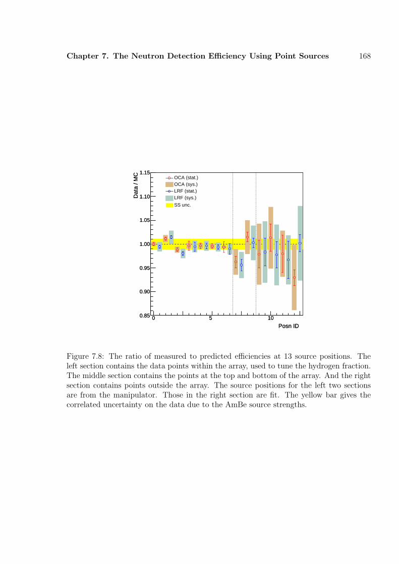
Chapter 7. The Neutron Detection Efficiency Using Point Sources 168
Posn ID0 5 10
Dat
a / M
C
0.85
0.90
0.95
1.00
1.05
1.10
1.15
Posn ID0 5 10
Dat
a / M
C
0.85
0.90
0.95
1.00
1.05
1.10
1.15OCA (stat.)OCA (sys.)LRF (stat.)LRF (sys.)
SS unc.
Figure 7.8: The ratio of measured to predicted efficiencies at 13 source positions. Theleft section contains the data points within the array, used to tune the hydrogen fraction.The middle section contains the points at the top and bottom of the array. And the rightsection contains points outside the array. The source positions for the left two sectionsare from the manipulator. Those in the right section are fit. The yellow bar gives thecorrelated uncertainty on the data due to the AmBe source strengths.

Chapter 7. The Neutron Detection Efficiency Using Point Sources 169
Figure 7.9: Comparison of 252Cf source data (red points) and Monte Carlo (green points)along the central, vertical axis of the detector [17]. Efficiencies were determined using theTSA analysis (see Appendix D). The error bars are statistical only.
7.4 The NC neutron detection efficiency
7.4.1 Result
Models of the dependence of the NC neutron detection efficiency on hydrogen fraction,
for the OCA and LRF geometries, were produced using Monte Carlo simulations. They
are shown in Figure 7.10. They were used to calculate the NC efficiencies corresponding
to the hydrogen fractions in Table 7.2.
The recommended value for the NC efficiency was taken to be the average of the
efficiencies found using 3 rings with the OCA and LRF geometries. The result was
0.2101 ± 0.0012.
The uncertainty include statistics, the uncertainty on the NCD geometry and the
uncertainty on the hydrogen fraction. It small magnitude reflects the small sensitivity of
the efficiency to latter two effects. The following section considers additional systematic
uncertainties that amount to 1.54% or 0.0032. The final NC neutron detection efficiency
was found to be 0.2101 ± 0.0035.

Chapter 7. The Neutron Detection Efficiency Using Point Sources 170
Hydrogen fraction0.0007 0.0008 0.0009 0.0010 0.0011 0.0012
Effi
cien
cy
0.200
0.205
0.210
0.215
0.220
0.225
0.230 / ndf 2χ 9.308 / 6
Prob 0.157p0 0.01309± 0.2375 p1 28.64± -33.34 p2 1.543e+04± 4600
/ ndf 2χ 9.308 / 6Prob 0.157p0 0.01309± 0.2375 p1 28.64± -33.34 p2 1.543e+04± 4600
Hydrogen fraction0.0007 0.0008 0.0009 0.0010 0.0011 0.0012
Effi
cien
cy
0.200
0.205
0.210
0.215
0.220
0.225
0.230 / ndf 2χ 1.01 / 6
Prob 0.9852p0 0.01309± 0.2376 p1 28.64± -33.1 p2 1.543e+04± 4053
/ ndf 2χ 1.01 / 6Prob 0.9852p0 0.01309± 0.2376 p1 28.64± -33.1 p2 1.543e+04± 4053
Figure 7.10: NC capture efficiencies as a function of hydrogen fraction for OCA geometry(left) and LRF geometry (right).
7.4.2 Systematic uncertainties
This section contains a list of systematic effects whose impact on the NC neutron detection
efficiency was investigated. They are summarised in Table 7.3.
• Hydrogen fraction and array geometry.
These were naturally taken into account in the procedure for fitting the hydrogen
fraction, described above.
• Acrylic vessel and light water.
Approximately 29% of NC neutrons were captured in the acrylic vessel and 6% in
the light water and so it was important to investigate the quality of the modelling
of these regions.
The geometry of the acrylic vessel was modelled in the Monte Carlo in some detail.
The most significant geometry parameter was the inner radius of the vessel, which
was 600.50 cm in the Monte Carlo, close to the true value of 600.54 cm. The only
significant omission was the simulation of the acrylic NCD anchor blocks but their
collective volume was small and their effect on the neutron detection efficiency was
expected to be negligible.
The modelling of the material of the acrylic vessel as a potential source of uncertainty
was studied by varying the density of hydrogen in the acrylic vessel in the Monte

Chapter 7. The Neutron Detection Efficiency Using Point Sources 171
Table 7.3: Systematic uncertainties on the Monte Carlo NC neutron detection efficiency.
Item Unc. (%)
Hydrogen fraction (fH) and string positions / tilts 0.57AV modelling ∼ 0.0Number of deuterons 0.2Counter dead regions 1.0Counter Ni wall thickness ∼ 0.0Counter gas pressure ∼ 0.03He cross section ∼ 0.0Residual NaCl concentration ∼ 0.0
NCD thresholds, data cleaning etc. 1.0
Total 1.54
Fractional change in AV H density-0.4 -0.3 -0.2 -0.1 -0.0 0.1 0.2 0.3 0.4
NC
neu
tron
cap
ture
effi
cien
cy
0.190
0.195
0.200
0.205
0.210
0.215
0.220
0.225
0.230 / ndf 2χ 5.584 / 7
Prob 0.589
p0 0.0002925± 0.2102
p1 0.001896± -0.001649
/ ndf 2χ 5.584 / 7
Prob 0.589
p0 0.0002925± 0.2102
p1 0.001896± -0.001649
Fractional change in AV H density-0.4 -0.3 -0.2 -0.1 -0.0 0.1 0.2 0.3 0.4
NC
neu
tron
cap
ture
effi
cien
cy
-210
-110
1O
2D
O2H
AVHe
3
Figure 7.11: The effect of absorption in the acrylic vessel on the NC neutron captureefficiency. The parameter varied is the density of hydrogen in the acrylic vessel. The lefthand plot shows the NC efficiency as a function of the change in density; the right handplot shows the variation of captures in various geometry regions.

Chapter 7. The Neutron Detection Efficiency Using Point Sources 172
Carlo to simulate a change in the ability of the acrylic vessel to absorb neutrons.
The results of these simulations are shown in Figure 7.11. The left hand plot shows
the variation in the NC neutron capture efficiency as a function of fractional change
in hydrogen density. A change in density of 30% resulted in a 0.02% change in
efficiency, indicating that there was an extreme insensitivity to neutron-absorbing
properties of the acrylic vessel. This was because the acrylic vessel and light water
contained large amounts of hydrogen and so were very strongly absorbing; the main
effect of varying the density was altering the depth the neutrons penetrated into the
acrylic vessel, rather than the probability that they were captured, having entered
the acrylic. This behaviour can be seen in the right hand plot of Figure 7.11, which
shows that when the density increased the 3He capture efficiency remained constant
but the fraction of neutrons capturing in the light water (i.e. those passing all the
way through the acrylic vessel) decreased. The modelling of the acrylic vessel was
neglected as a source of uncertainty in the Monte Carlo.
Neutron propagation in the light water region was described by a dedicated ENDF
table in MCNP [68] and it captured a relatively small fraction of neutrons. There
was no reason to suspect any mis-modelling would have had any significant effect,
so it too could be neglected as a source of uncertainty.
• Counter end regions.
If the uncertainty on the size of the end regions was conservatively estimated at 50%,
there would be an uncertainty on the active volume of 3He gas, and therefore on the
neutron detection efficiency, of 1%. This was taken as a systematic uncertainty.
• Counter nickel wall thickness.
There was no significant uncertainty on the nickel wall thicknesses or on the overall
mass of nickel in the detector. The thicknesses of the counter walls varied in the
Monte Carlo based on measurements the masses and lengths of the nickel tubes
from which the counters were constructed (see Section 4.3.2). The counter walls
captured 2.2% of NC neutrons or around 1/10th of the number capturing on 3He;
a 0.5% change in the 3He capture efficiency would require an implausible error of
∼ 5% in the mass of Nickel. No systematic uncertainty was assigned.
• Counter gas pressure.
There was some variation in the pressure of the 3He gas from counter to counter.
The limit on this variation was derived from the tolerance on the counter gain of
3%. The gain of each counter was measured before deployment and if it fell outside
this tolerance it had to be refilled. The gain was very sensitive to gas pressure and

Chapter 7. The Neutron Detection Efficiency Using Point Sources 173
Robertson [135] estimated that the gain tolerance of 3% was equivalent to a gas
pressure tolerance of 0.5%.
The effect of such a change on the NC efficiency was expected to be negligible as the
large 3He cross section meant that the counters were effectively black to neutrons.
A small change in the gas pressure would have changed the mean capture depth but
would have had little effect on the efficiency.
A leak of 3He gas from a counter would have been manifest as a change in gain of
the counter or by the appearance of 3He in the heavy water. No systematic gain
changes were found and a 3He detection system found no evidence of 3He in the
heavy water. The 3He detection system, which was integrated into the existing
water systems, searched for a mass-3 signal in exhaust gas from the D2O degasser.
It is described in more detail in [136].
No systematic uncertainty was assigned.
• 3He cross section.
This was checked in Section 4.2.1 and found to be set correctly in the Monte Carlo.
No systematic uncertainty was assigned.
• Residual NaCl concentration.
This was considered in Section 4.2.2. The small effect of the residual salt concen-
tration is likely to have been calibrated out by the hydrogen fraction tuning (the
effect on neutron propagation would be indistinguishable from a slightly increased
hydrogen fraction) and so no correction factor was applied. Likewise no systematic
uncertainty was assigned.
• Number of deuterons.
The density of the D2O in the Monte Carlo was found to be too small by 1.3%.
The effect of this on the detection efficiency is likely to have been tuned away by
the hydrogen fraction fitting. Taking this into account Robertson [135] estimated a
conservative uncertainty of 0.2%.
• Threshold efficiencies, data cleaning etc.
The effect of the NCD threshold efficiencies and other inefficiencies on the NC
efficiency was conservatively estimated by Guillian [132] to be 1%.

Chapter 7. The Neutron Detection Efficiency Using Point Sources 174
7.5 Other neutron detection efficiencies
Most of this thesis has been concerned with calculating the neutron detection efficiency
for NC neutrons in the NCD array. The PMT efficiency for NC neutrons was also required
as well as the PMT and NCD efficiencies for all classes of background neutron. These
efficiencies were less important, and therefore given less attention, because of the small
number of neutrons detected in each case and, for the backgrounds, the large uncertainties
on the numbers of neutrons produced in the detector.
Efficiencies were taken directly from Monte Carlo and systematics assigned based
on the result for NC neutrons in the NCD array. The systematic on the NCD efficiencies
was taken to be the same as the uncertainty on the NC NCD efficiency (1.54%). The
systematic on the PMT efficiencies was 1.17%, which was the part of the NCD systematic
that did not relate directly to detection (as opposed to capture) of neutrons by the NCD
array; the main contribution removed was the one due to the size of the NCD end regions.
Systematic uncertainties associated with energy reconstruction, position reconstruction,
cut acceptance etc. were naturally handled in the fits to extract the neutrino fluxes
described in the next chapter. The results were:
Background PMT eff. NCD eff.
Value Unc. Value Unc.
K2 PD 0.0641 0.0008 0.2603 0.0047K5 PD 0.0700 0.0009 0.3039 0.0054Bulk PD 0.0595 0.0010 0.4095 0.0071
NC 0.0485 0.0006
The efficiencies for the acrylic vessel (α,n) neutrons and others originating at or near the
acrylic vessel were evaluated in a separate study by [61].
7.6 Summary
This chapter has described theoretical determinations of the neutron detection efficiencies
for neutrons from various sources in the PMT and NCD arrays. The NCD NC neutron
detection efficiency was found to be
0.2101 ± 0.0035

Chapter 7. The Neutron Detection Efficiency Using Point Sources 175
where the systematic contributions to the uncertainty are given in Table 7.3. The non-
NCD-non-NC efficiencies are given in the table above.

Chapter 8
Measuring the NC flux
If your experiment needs statistics, you ought to have done a better experiment.
ERNEST RUTHERFORD
This chapter describes the statistical extraction of the 8B solar neutrino fluxes from
the NCD phase data. A maximum likelihood technique was used to estimate the
numbers of neutrino candidate events that were due to neutrino interactions (CC, ES or
NC) and backgrounds. Events were described by a set of observable parameters, such as
event energy or radius, and the data were fit to a combination of probability distribution
functions (PDFs) for each of the signals in each of the observables. PDFs were constructed
using Monte Carlo or calibration data.
The numbers of events belonging to each class of background were constrained in
the fit by external measurements. Systematic uncertainties, such as neutron detection
efficiencies, which were also constrained by external measurements, were either allowed
to float in the fit, as nuisance parameters, or the fit was repeated with the parameters
set to the positive and negative 1 σ limits allowed by the external measurements. Where
possible, systematic uncertainties were floated, as this allowed the data to constrain their
values and allowed central values to move within their constraints.
This chapter begins with the maximum likelihood method and the particular for-
malism used in this analysis. Following this is a description of the way that the systematic
uncertainties were handled and of the analysis code. Finally the results are presented -
the neutrino fluxes and the inferred solar neutrino mixing parameters.
176

Chapter 8. Measuring the NC flux 177
8.1 Fitting using maximum likelihood
8.1.1 Overview
The maximum likelihood technique is a procedure for estimating model parameters. It
is widely used because of its simplicity and ideal asymptotic behaviour - in the limit of
a large number of data points uncertainties on fit parameters take their smallest possible
values and fits are unbiased [137].
The data is described by a set of observables and the model parameter values are
those which maximise the probability of the observed data. Parameter uncertainties are
assigned using the variation of the probability with parameter value about the best fit
point, with all other parameters unconstrained.
In this analysis the neutrino data were described as a sum of CC, ES, NC and
background events. Each of these classes of event is referred to as a signal ; the fit
parameters were the numbers of events (or equivalently fluxes) corresponding to each
signal. The observables were quantities measured by SNO, such as event energy.
8.1.2 The NCD phase formalism
The likelihood function L is given by
L =
Nd∏
d=1
f(xd; θ) (8.1)
where Nd is the number of data events and f(xd; θ) is the PDF giving the probability of
measuring observable values xd, given a set of parameters θ. The best fit parameters are
those which maximise L.
In this analysis the PDF was given by
f(xd; θ) =
Ns∑
s=1
ns
Ndfs(xd) (8.2)
where Ns is the number of signals, ns is the number of data events belonging to signal s,
Nd is the number of events in the data set, and fs(xd) is a PDF obtained from Monte Carlo
or calibration data, which gave the probability of measuring xd for signal s. Substituting

Chapter 8. Measuring the NC flux 178
Eq. (8.2) into Eq. (8.1) gives
L =
Nd∏
d=1
Ns∑
s=1
ns
Ndfs(xd) (8.3)
The total number of events Nd is distributed about the expected number of events µ0
according to Poisson statistics. The probability of observing Nd given µ0 can be included
in the likelihood function in what is known as the extended maximum likelihood method.
Eq. (8.3) becomes
L =µNd
0 e−µ0
Nd!
Nd∏
d=1
Ns∑
s=1
ns
Ndfs(xd) =
e−µ0
Nd!
Nd∏
d=1
µ0
Ns∑
s=1
ns
Ndfs(xd) (8.4)
Rather than maximise L it is conventional to minimise the negative log-likelihood L =
− logL. The logarithm is introduced because likelihoods can take large absolute values
and the minus sign because widely used codes minimise rather than maximise functions.
Taking the negative logarithm of Eq. (8.4) gives
L = −Nd∑
d=1
log
(
Ns∑
s=1
µ0ns
Ndfs(xd)
)
+ µ0 + log(Nd!) (8.5)
The expected number of events µs of signal s can be written
µs = µ0ns
Nd
(8.6)
such that
µ0 =Ns∑
s=1
µs (8.7)
Substituting these into Eq. (8.5) gives
L = −Nd∑
d=1
log
(
Ns∑
s=1
nsfs(xd)
)
+Ns∑
s=1
ns (8.8)
where the constant term in Nd has been omitted.
If external measurements provide constraints on any of the fit parameters then
constraint terms may be added to the likelihood. Eq. (8.8) becomes
L = −Nd∑
d=1
log
(
Ns∑
s=1
nsfs(xd)
)
+
Ns∑
s=1
ns −1
2
Np∑
p=1
(
λp − λp
σp
)2
(8.9)

Chapter 8. Measuring the NC flux 179
where λp is the central value of the Gaussian constraint on parameter λp and σp is its
width. Constraints may also be applied to parameters used when forming the PDFs
fs(xd), such as the energy scale, or in the conversion of fluxes into numbers of events,
such as neutron detection efficiencies.
It was physically interesting to make no assumption on the energy spectra of CC
and ES events, which was equivalent to making no assumption on the 8B neutrino energy
spectrum. The number of events in each energy bin was treated as an independent fit
parameter and the probability inside each energy bin taken to be constant. This type of
fit is referred to as an unconstrained fit. The PDF f(xd; θ) becomes
f(xd; θ) =∑
s = CC,ES
(
Nspec∑
i=1
nsifsi(xd)
)
+∑
s 6=CC,ES
nsfs(xd) (8.10)
where Nspec is the number of CC and ES spectral bins. The negative log-likelihood L is
modified accordingly.
In this analysis there were two data streams from largely independent detectors - the
PMT and NCD arrays. Some signals were unique to each detector, such as CC neutrino
events in the PMTs and alpha backgrounds in the NCD, while others could be recorded
by both detectors, such as NC and photodisintegration background neutrons. With two
data streams the negative log-likelihood becomes
L = LPMT + LNCD (8.11)
LPMT = −Nd∑
d=1
log
(
Ns∑
s=1
nsfs(xd)
)
+Ns∑
s=1
ns −1
2
Np∑
p=1
(
λp − λp
σp
)2
(8.12)
LNCD = −N ′
d∑
d=1
log
(
N ′s
∑
s=1
n′sf
′s(xd)
)
+
N ′s
∑
s=1
n′s −
1
2
N ′p
∑
p=1
(
λ′p − λ′
p
σ′p
)2
(8.13)
where the unprimed quantities refer to to the PMT stream and primed quantities to the
NCD stream. When a pair of event classes have a common source, the event numbers ni
and n′i are not independent and are related by
ni = Fi × Si × Ei (8.14)
n′i = Fi × S ′
i × E ′i (8.15)
where Ei and E ′i are the numbers of events expected to be observed in each stream, given
predictions for the source production rate and detector response; Si and S ′i are corrections

Chapter 8. Measuring the NC flux 180
Table 8.1: Summary of signals included in the fit. The last two columns indicate whetherthe signal is present in the PMT and NCD streams. PD stands for photodisintegration.
Type Name Events Data
PMT NCD
Physics CC CC neutrino yesES ES neutrino yesNC NC neutrino yes yes
Neutron AV AV (α,n) + H2O PD n yes yesbackgrounds K2 PD K2 hotspot PD n yes yes
K5 PD K5 hotspot PD n yes yesNCD PD NCD Ni PD n + (α,n)17/18O yes yesUniform D2O PD n yes yesn-like Atmos. ν + NCD cable PD n + 16N yes yes
NCD-only Alphas Alphas from NCD components yesbackgrounds J3 J3 instrumentals yes
N4 N4 instrumentals yes
to Ei and E ′i to account for the change in the expected number of events after application
of a shift in a systematic parameter; and Fi is the fraction of the expected number of
events observed. In general, it is the quantities Fi, referring to fluxes or source terms,
which are fit for, rather than numbers of events.
Uncertainties on fit parameters are defined as the variations in parameter values
that cause increases in the negative log-likelihood of 0.5. For example, the uncertainty
δns on ns is defined by
L(ns ± δns) = L(ns) + 0.5 (8.16)
8.2 Probability distribution functions
8.2.1 Signals and backgrounds
A list of the signals included in the likelihood function is given in Table 8.1. They were
grouped into three categories:
• Physics signals.

Chapter 8. Measuring the NC flux 181
Table 8.2: Neutron detection efficiencies.
Signal PMT NCD
Val. Unc. Val. Unc.
NC 0.0485 0.0006 0.211 0.007
AV 0.0068 0.0113
K2 0.0641 0.0008 0.2603 0.0027K5 0.0700 0.0009 0.3034 0.0027Bulk 0.0595 0.0010 0.4095 0.0032Uniform See NC See NC
The physics signals were events due to CC, ES and NC neutrino interactions. CC
and ES events were detected by the PMT array and NC events by both the PMT and
NCD arrays. All signals were fit as solar neutrino fluxes, which were converted into
numbers of events using Eq. (8.14) and Eq. (8.15), to allow the likelihood function
to be evaluated.
• Neutron and neutron-like backgrounds.
There were three main sources of neutrons in the detector, other than NC interac-
tions: deuteron photodisintegration by gammas from U and Th in the H2O, D2O,
bulk materials of the NCD array, the acrylic vessel, the two NCD hotspots and the
NCD cables; (α,n) reactions in the acrylic vessel; and interactions of atmospheric
neutrinos in the D2O. These produced events in both the PMT and NCD arrays.
In addition, there were two non-negligible sources of neutron-like events in the
PMT array only: the decay of 16N produced in the reactions 16O(µ−,νµ)16N and16O(n,p)16N; and atmospheric neutrino interactions other than those producing neu-
trons.
In previous SNO analyses most neutron and neutron-like backgrounds were deducted
from the fit number of NC events, but because there were two detectors in the NCD
phase they now had to be included in the fit. This was because, for some of the
backgrounds, the relative event rates between the detectors and radial distributions
differed from NC neutrons. The differences in radial profiles were not large enough
to allow the data to help significantly in distinguishing the backgrounds from each
other, or from NC neutrons, but they had the potential to bias the fit results.
The backgrounds were divided into 6 groups, each containing backgrounds with
similar detection efficiencies and with similar distributions in the observables. In
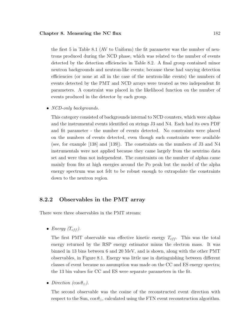
Chapter 8. Measuring the NC flux 182
the first 5 in Table 8.1 (AV to Uniform) the fit parameter was the number of neu-
trons produced during the NCD phase, which was related to the number of events
detected by the detection efficiencies in Table 8.2. A final group contained minor
neutron backgrounds and neutron-like events; because these had varying detection
efficiencies (or none at all in the case of the neutron-like events) the numbers of
events detected by the PMT and NCD arrays were treated as two independent fit
parameters. A constraint was placed in the likelihood function on the number of
events produced in the detector by each group.
• NCD-only backgrounds.
This category consisted of backgrounds internal to NCD counters, which were alphas
and the instrumental events identified on strings J3 and N4. Each had its own PDF
and fit parameter - the number of events detected. No constraints were placed
on the numbers of events detected, even though such constraints were available
(see, for example [138] and [139]). The constraints on the numbers of J3 and N4
instrumentals were not applied because they came largely from the neutrino data
set and were thus not independent. The constraints on the number of alphas came
mainly from fits at high energies around the Po peak but the model of the alpha
energy spectrum was not felt to be robust enough to extrapolate the constraints
down to the neutron region.
8.2.2 Observables in the PMT array
There were three observables in the PMT stream:
• Energy (Teff).
The first PMT observable was effective kinetic energy Teff . This was the total
energy returned by the RSP energy estimator minus the electron mass. It was
binned in 13 bins between 6 and 20 MeV, and is shown, along with the other PMT
observables, in Figure 8.1. Energy was little use in distinguishing between different
classes of event because no assumption was made on the CC and ES energy spectra;
the 13 bin values for CC and ES were separate parameters in the fit.
• Direction (cos θ⊙).
The second observable was the cosine of the reconstructed event direction with
respect to the Sun, cos θ⊙, calculated using the FTN event reconstruction algorithm.

Chapter 8. Measuring the NC flux 183
Energy (MeV)0.4 0.5 0.6 0.7 0.8 0.9 1.0 1.1 1.2 1.3 1.4
Energy (MeV)0.4 0.5 0.6 0.7 0.8 0.9 1.0 1.1 1.2 1.3 1.4
NeutronsAlphas
J3 instr.N4 instr.
Figure 8.1: Signal PDFs. The distributions in the PMT observables for CC, ES and NCare shown in energy (top left), cosine of reconstructed direction with respect to that ofthe Sun (top right) and radius (centre left). Note that the shapes of the energy PDFs forCC and ES events were allowed to float in the fits. The background radial distributionsare shown centre right. The bottom plot shows the distributions in the NCD observableshaper-ADC energy. Normalisations should be considered arbitrary.

Chapter 8. Measuring the NC flux 184
Table 8.3: High level cuts.
Stream Parameter Cut
PMT Teff 6 < Teff < 20ρ 0 < ρ < (550
600)3
cos θ⊙ −1.0 < cos θ⊙ < 1.0β14 -0.12 < β14 < 0.95ITR ITR > 0.55
NCD EADC 0.4 < EADC < 1.4String Cut 4He strings 3, 10, 20, 30
Cut bad strings 0, 1, 8, 18, 26, 31 [140]
It was binned in 25 bins between -1 and 1. cos θ⊙ placed a strong constraint on the
number of ES events.
• Radius (ρ).
The third observable was event radius in the form of the radial parameter ρ =
(r/rAV )3, where rAV = 600 cm was the nominal radius of the acrylic vessel. ρ was
binned in 10 bins from 0 to (550/rAV )3. The volume within 550 cm is known as
the fiducial volume. ρ provided some ability to distinguish NC from CC and ES
events - the former had a non-uniform distribution because the NCD array mainly
absorbed neutrons at small radii and the acrylic vessel at larger radii.
PMT PDFs were generated using binned Monte Carlo events. The overall PMT PDF was
factorised into two parts
f(Teff , cos θ⊙, ρ) = f(Teff , ρ) × f(cos θ⊙)
The reason that a full 3 dimensional PDF was not used was to increase the number of
PDF events in each bin. This was desirable because it reduced the potential for fit biases
by reducing the effect of statistical fluctuations on the PDF shapes. For example, moving
from 3D to 2D×1D increased the average number of events per bin in the NC PDF (the
physics signal with the least statistics) from 60 to 1500. However, any factorisation of this
sort did have the potential to introduce a bias because the PDF then explicitly neglected
the correlations between some of the observables. Tests (see Section 8.5.2) were performed
to establish that correlations between cos θ⊙ and either Teff or ρ did not cause biases in
the fit fluxes.

Chapter 8. Measuring the NC flux 185
8.2.3 Observables in the NCD array
There was a single observable in the NCD stream:
• Energy (EADC).
The NCD observable was shaper-ADC energy EADC in which neutrons, alphas, J3
and N4 instrumentals had different distributions. The energy range was from 0.4
to 1.4 MeV in 20 bins. This range included the neutron peak and a region above
∼ 0.8 MeV where there were no neutron events.
The lower energy cut resulted in sacrifice of the 6% of neutron events occurring below
0.4 MeV but the loss of statistics was more than compensated for by removing the
need to model the alpha spectrum down to these energies. An added advantage was
that it excluded the region where most J3 and N4 instrumental events occurred; the
energy spectrum of these events was difficult to model.
The region above 0.8 MeV was included to provide information on the alpha back-
ground, which helped constrain its magnitude underneath the neutron peak. The
reason alpha events above 1.4 MeV were not included, even though they would have
provided more statistics for the constraint, was because of the demands it would
have placed on the ability to model the alpha spectrum over a large energy range.
Neutrons for all sources had identical energy spectra and so the NCD array could not
distinguish between NC and background neutrons. This ability would have been provided
by a spatial variable as not all classes of background neutron produced captures uniformly
distributed over the array. Various possibilities were considered including a 40 string PDF
and 6 ring PDFs where the rings of strings were centred on the detector z-axis or on the
strings containing the hotspots. However, given the strength of the external constraints
on the background neutron production rates there was little to gain from the added
complexity of including a spatial PDF. This is discussed further in Section 8.5.2.
The neutron energy PDF was generated using data from the 2005 24Na measurement.
The nominal alpha PDF was generated using Monte Carlo. The following analytical PDFs
from [139, 141] were used for the J3 and N4 instrumentals
f ′J3(EADC) = Ce
−“
EADC−βJ30.34 EADC
”2
(1 + erf(−2.0(EADC − βJ3)) (8.17)
f ′N4(EADC) = Ce
−“
EADC−βN4−19.6 EADC
”2
(1 + erf(−1.59(EADC − βN4)) (8.18)

Chapter 8. Measuring the NC flux 186
where βJ3 = 0.4584 ± 0.0262 and βN4 = 0.0257 ± 0.0138. These functional forms had
no physical basis other than that they provided good fits to samples of the events. The
production mechanism for J3 and N4 instrumental events has not been identified. The
particular characteristics of these events are described in the next section.
There was a period during the development of this analysis when the pulse shapes of
alpha events could not be simulated satisfactorily and it was unclear how to treat events
such as the J3 and N4 instrumentals. The particular concern with the alpha simulation
was that, with no Monte Carlo, there was no reliable way of determining the shape of the
background underneath the neutron peak, particularly as the radioactivity on the 4He
strings turned out to be rather unrepresentative, in its composition, of that of the 3He
strings. The collaboration actively considered running with a neutron-absorbing isotope,
such as Gadolinium, dissolved in the heavy water to remove the neutron signal from the
NCDs and allow a direct measurement of the background. A study of the statistical power
of such a measurement is described in Appendix H.
These concerns were allayed by improvements in the understanding of alpha pulse
formation - particularly by Wan [142] who discovered that alpha events with anomalously
long pulses originated from radioactivity on the NCD wires - and by exhaustive, negative
searches for non-physics events on other strings (see, for example, [143]). The Monte
Carlo used for the alpha background in this analysis could reproduce all classes of alpha
pulse shape and the energy spectrum of the 4He strings.
8.2.4 Instrumental and high level cuts
Neutrino candidate events in the PMT stream were events that passed a set of low level
instrumental cuts and a set of more sophisticated high level cuts on the following param-
eters:
• ITR > 0.55
The in-time ratio (ITR) was a measure of the proportion of the PMT hits in an
event arriving in the prompt peak; larger values corresponded to a larger proportion.
This cut was effective at removing low energy background events that occurred in
the light water but mis-reconstructed inside the fiducial volume.
• −0.12 < β14 < 0.95
The parameter β14 was a measure of event isotropy. It was constructed from the βl
parameters, which were the average values of the Legendre polynomials Pl of the

Chapter 8. Measuring the NC flux 187
cosine of the angles, with respect to the reconstructed position, between each pair of
PMT hits in an event [144]. β14 = β1 +4β4 increased with increasing event isotropy.
The range was chosen to include all physics events originating within the acrylic
vessel.
There were 146 431 247 raw PMT triggers during the NCD phase, composed mainly of
instrumental and low energy background events. 2 381 of these were selected as neutrino
candidates.
In the NCD stream there was again a set of low level instrumental cuts. There were
no high level cuts but events on all 4He strings and on 6 3He strings [140] were removed.
The 3He strings that were cut were:
• K5 (hotspot and leak).
This string suffered from a slow leak of 3He from one of the counters into an in-
terspace region which caused distortions to the energy spectrum that varied slowly
over the NCD phase; this made energy calibration difficult. In addition, K5 was the
site of one of the radioactive hotspots and registered 47% of the detected neutron
events arising from it.
• K2 (hotspot and electrical disconnect).
This string suffered from intermittent electrical disconnects and consequently had a
live time that was difficult to quantify. It was also the site of one of the radioactive
hotspots and registered 47% of the detected neutron events arising from it.
• M8 (electrical disconnect).
This string suffered a permanent electrical disconnect.
• J3 (neutron-like instrumentals).
This string contained an excess of the low energy events referred to as J3 instrumen-
tals that had pulse shapes that were difficult to distinguish from neutrons. They
had a different energy spectrum to neutrons, peaking much lower in energy. Both
the pulse shapes and energy distributions were consistent with the events being be-
tas but no source has been identified. The string itself was removed and a J3 PDF
included in the fit to pick up these events if they occurred on other strings.
• N4 (neutron-like instrumentals).
Like string J3, string N4 contained low energy instrumental events and they were
dealt with in the same way.

Chapter 8. Measuring the NC flux 188
• K7 (gain changes).
This string suffered from sporadic gain changes that made its energy calibration
unreliable.
The were 1 417 811 raw NCD triggers during the NCD phase. After instrumental cuts
this was reduced to 91 636 and, after removal of strings and imposing the energy cut, to
7 302 events, of which ∼ 80% were alphas.
8.3 Fluxes and events
For classes of event detected in both the PMT and NCD data streams the fit parameter
was the flux of neutrinos or the number of background neutrons produced rather than
the number of events in each stream. However, numbers of events were required to
evaluate the likelihood function in Eq. (8.11) so conversion factors were required. This
section describes how the quantities E and E ′, which governed the conversion of fluxes or
production rates into events via Eq. (8.14) and Eq. (8.15), were calculated.
The signals that were fit as fluxes or neutrons produced were the CC, ES and NC
neutrino events and the 5 groups of neutron backgrounds. The expected numbers of
events for each, in each stream, were given by
ECC,ES = Nmc · (ηtarget · ηnuclei · rgeom · εcut · tcut) (8.19)
EPMTNC = Rmc · εPMT
nc · Tlive · (ω · r⊙ · εcut) (8.20)
E ′NCDNC = Rmc · εNCD
nc · Tlive · (ω · r⊙ · εcut) (8.21)
EPMTbkgrd = Rgen · εPMT
bkgrd · Tlive · (εcut) (8.22)
E ′NCDbkgrd = Rgen · εNCD
bkgrd · Tlive · (εcut) (8.23)
The expression for CC and ES has a slightly different form than the one for NC. This
is because for CC and ES the Monte Carlo is used to predict the number of events for
each unit of neutrino flux, whereas for NC that relationship is measured via the neutron
detection efficiencies.
The values of the quantities in these expressions are given in Table 8.4 or elsewhere,
as indicated below. They are defined as follows:

Chapter 8. Measuring the NC flux 189
• Nmc
The number of Monte Carlo events within cuts per standard solar model assuming
an undistorted 8B neutrino energy spectrum. The model used was BP2000 [145],
which predicted a 8B flux of 5.145 × 10⁶ ν cm2 s−1.
• Rmc
NC neutron production rate of 13.2745 day−1 predicted, by SNOMAN, to correspond
to a flux of 5.145 × 10⁶ ν cm2 s−1.
• ηtarget
A correction for the number of deuteron or electron targets, which differed slightly
between data and Monte Carlo.
• ηnuclei
A correction for neutrino interactions on oxygen and nickel that were not included
in the Monte Carlo.
• ǫgeom
A correction for the number of CC and ES Monte Carlo events aborted during
simulation because of errors in the SNOMAN geometry code [146].
• εcut
In the PMT stream this was a correction for the difference in cut efficiencies between
data and Monte Carlo. In the NCD stream this included contributions due to the
sacrifice of neutrons below 0.4 MeV and instrumental cuts.
• εPMT/NCDnc/bkgrd
Neutron detection efficiencies (see Table 8.2).
• tcut
A correction for the difference in livetimes between data and Monte Carlo.
• Tlive
The NCD phase livetime of 385.17 ± 0.14 days [147].
• r⊙
A correction to the number of predicted NC events to account for the mean orbital
radius during data taking.

Chapter 8. Measuring the NC flux 190
Table 8.4: Correction factors used when converting fluxes into numbers of events.
Correction CC ES NC NC PD PD
Symbol Description PMT NCD PMT NCD
r⊙ Mean orbital radius 1 1 1.00101 1.00101 1 1ηtarget Number of D / e− 1.01218 1.0131 1 1 1 1ηnuclei CC interactions on O, Ni 1.0078 1 1 1 1 1εcut Cut acceptance 0.9917 0.9917 0.9917 0.862 0.9917 0.862tcut Livetime correction 0.9804 0.9804 1 1 1 1εgeom Geometry errors 1.0123 1.0073 1 1 1 1ω Radiative correction 1 1 1/1.024 1/1.024 1 1
Net correction 1.00398 0.99219 0.96944 0.84265 0.9917 0.862
• ω
A correction to account for radiative corrections to the neutrino interaction cross
sections as implemented in the Monte Carlo. These were small and so applied ‘on
average’ rather than event-by-event.
• Rgen
The measured background neutron production rates (see Table 8.5).
After application of all these correction factors and using the central values of all sys-
tematic parameters, the numbers of events expected for 1 standard solar model (a flux of
5.145 × 10⁶ ν cm−2 s−1) were 5583.670 CC events, 480.471 ES events, 240.398 NC events
in the PMT array and 909.071 NC events in the NCD array.
8.4 Systematic uncertainties
8.4.1 Using the data
There were two classes of systematic uncertainty in this analysis: the first was uncertain-
ties on PDF shapes and the second was uncertainties on the conversions between fluxes
and number of events. The detector energy scale is an example of the former and the
neutron detection efficiencies are examples of the latter. The values and uncertainties on
systematic parameters were assessed using calibration data.

Chapter 8. Measuring the NC flux 191
Table 8.5: Numbers of background events produced and detected. For the neutron back-grounds the fit constraints were the numbers produced and for the neutron-like back-grounds the fit constraints were the numbers detected.
Background Produced PMT detected NCD detected
Value Unc. Value Unc. Value Unc.
AV 2719.30 1359.65 18.34 9.17 26.49 13.24K2 146.37 23.50 9.30 1.50 32.84 5.27K5 120.56 13.87 8.37 0.96 31.53 3.63Bulk 78.27 36.51 4.62 2.16 27.63 12.89Uniform 170.59 25.88 8.21 1.25 31.03 4.71
n-like 27.99 5.20 36.12 15.60
Total 76.82 10.98 185.63 25.46
In previous SNO 8B flux analyses systematic uncertainties were handled using the
shift and re-fit method. In this technique the full fit, with all parameters free, was run
using the central values of all systematic parameters and then again when each systematic
was shifted to its ±1σ limits. The changes in the flux values due to each systematic were
assumed to be independent and were added in quadrature.
This method is not ideal for a number of reasons, all stemming from the fact that
it does not use the information provided by the neutrino data. For example, if that data
strongly favoured one value of a systematic, the ±1σ shifts, derived from the calibration
data, might change the fit likelihood by much more than 0.5, leading to an overestimate of
the error. The shift-and-refit procedure also does not allow the central value systematics
to move, given the information provided by the data. The ideal method is one in which
all systematics are included as parameters in the fit, subject to constraints from external
measurements. This is referred to as the floating systematics method.
The technical challenges involved in floating systematics in fits to SNO data can be
substantial because most PDFs are binned and constructed from large numbers of Monte
Carlo events. During the fit every time the value of a systematic parameter associated with
a PDF shape is changed then the PDFs need to be rebuilt. As well as being CPU-intensive
this procedure can cause convergence problems because discontinuities are introduced into
the likelihood space when events move between bins.
Three different approaches were taken to the problem of handling systematic uncer-
tainties in the NCD flux analysis, in three independent codes (described in Section 8.5.1).

Chapter 8. Measuring the NC flux 192
Table 8.6: PDF shape systematic uncertainties with their one sigma constraints. Theunits are cm for distances and MeV for energies.
Stream Param. Description Value Unc. Type
PMT axo x-coordinate shift 0.0 4.0 Shift
ay0 y-coordinate shift 0.0 4.0 Shift
az0 z-coordinate shift 5.0 4.0 Shift
bxyz0 xyz-coordinate scale 0.000 0.009 Shift
cxy0 xy-resolution constant 0.06546 0.02860 Shift
cxy1 xy-resolution linear -0.00005501 0.00006051 Shift
cxy2 xy-resolution quadratic 3.9 × 10⁻⁷ 2.0 × 10⁻⁷ Shift
cz0 z-resolution constant 0.07096 0.02805 Shift
cz1 z-resolution linear 0.0001155 0.00008251 Shift
a⊙0 Angular resolution 0.00 0.06 ShiftbT0 Energy scale 0.0000 0.0109 Shift
cT0 Energy resolution (n) 0.0119 0.0104 Shift
cT0 Energy resolution (e−) 0.0162 0.0142 Shift
NCD bA0 Neutron energy scale 0.0 0.01 Shift
cA0 Neutron energy resolution 0.0 +0.01 Shift
bα0 Alpha Po depth variation 0 1 Float
bα1 Alpha Bu depth variation 0 1 Float
bα2 Alpha drift time variation 0 1 Float
bα3 Alpha avalanche width offset variation 0 1 Float
bα4 Alpha avalanche grad. offset variation 0 1 Float
bα5 Alpha Po/Bu fraction variation 0 1 Float
bα6 Alpha ion mobility 0 1 Float
αJ3 J3 3NA shape parameter 0.458419 0.026243 FloatαN4 N4 3NA shape parameter 0.025720 0.013758 Float
In the analysis reported here systematics associated with the shapes of binned PDFs were
handled using the shift and re-fit method but all others - those associated with the shapes
of analytical PDFs and with the conversion of fluxes into numbers of events were floated
in the fit, subject to their external constraints.
The systematic parameters in this analysis are shown in Table 8.6. For systematics
handled using the shift and re-fit method the values of the systematics in the table were
used for the central fits. Note that a large number of the values differed from zero. The
PDF shape systematics are described in turn in the following sections.

Chapter 8. Measuring the NC flux 193
8.4.2 PMT stream
• Energy.
Scale and resolution uncertainties associated with the estimated event energy were
calculated by [148]. The energy used in the fit T ′eff was related to the raw estimated
energy Teff by
T ′eff = (1 + bT
0 ) Teff + cT0 (Teff − Teff,gen) (8.24)
where bT0 is the energy scale, cT
0 is the energy resolution and Teff,gen is the energy
of the generated Monte Carlo event. The energy scales for neutrons and electrons
were different but completely correlated; they differed because of the different char-
acteristics of the neutron and electron (16N) calibration sources and were correlated
because the detector was the same for both. In the shift-and-refit-procedure bT0 and
cT0 were moved independently to their 1 σ limits. In the shifts of bT
0 the electron and
neutron energy scales were shifted together.
• Vertex.
Vertex offset, scale and resolution uncertainties arose from the knowledge of the
optical response of the detector and the performance of the FTN fitter [59]. Coor-
dinates used in the fit were related to the reconstructed positions by
x′ = ax0 + (1 + bxyz
0 ) x + (cxy0 + cxy
1 z + cxy2 z2) (x − xgen) (8.25)
y′ = ay0 + (1 + bxyz
0 ) y + (cxy0 + cxy
1 z + cxy2 z2) (y − ygen) (8.26)
z′ = az0 + (1 + bxyz
0 ) z + (cz0 + cz
1z) (z − zgen) (8.27)
where ax0 , a
y0, a
z0 are coordinate shifts, bxyz
0 is vertex scaling common to each co-
ordinate, cxy0 , . . . , cz
1 are resolution parameters and xgen, ygen and zgen are event
generation points in the Monte Carlo. The resolution parameters were correlated
but in this analysis, where they were handled by the shift and re-fit procedure, they
were treated as being independent. Vertex resolution uncertainties were so small
(see results) that neglecting the correlation between the parameters cannot have
affected the final uncertainties.
• Angular resolution.
The PMT angular resolution systematic uncertainty was applied only to the ES
signal, because only that signal had a distribution in cos θ⊙ that was not slowly
varying; CC and NC PDFs in this parameter were close to uniform. A convenient

Chapter 8. Measuring the NC flux 194
parametrisation of the uncertainty was derived by [149], in which the value cos θ⊙
used in the fit was related to that reported by the position fitter by
cos θ′⊙ = 1 + (1 + c⊙0 ) (cos θ⊙ − 1) (8.28)
During the shift and re-fit procedure if cos θ⊙ for a particular event was pushed
outside the physical region −1 < cos θ⊙ < 1 then the event was assigned a random
value of c⊙0 between -1 and 1. This was to avoid artificial peaks being created in
the first and last bins because of pile up events. The number of events affected was
negligible, less than 1/100th of a percent.
8.4.3 NCD stream
• Neutron energy.
Scale and resolution systematic uncertainties were assigned to the neutron shaper-
ADC energy PDF in an analysis by [150]. The energy used in the fit was related to
calibrated neutron energy from the 24Na measurement by
E ′ADC = (1 + bA
0 ) EADC + g(0, cA0 ) EADC (8.29)
where bA0 is the scale and cA
0 is the resolution. The neutron energy PDF was unique
in being formed from calibration data and thus had a resolution that could only be
broadened. The broadening was done by sampling from a Gaussian g(0, cA0 ) with
mean 0 and width cA0 .
• Alpha energy.
The NCD alpha energy PDF was generated using Monte Carlo [151, 152]. Seven
systematic uncertainties, each accounting for the uncertainty on a different Monte
Carlo input parameter, were each assigned a second-order polynomial re-weighting
factor fs(EADC) that parametrised the effect of the uncertainty on the PDF. Each
polynomial was multiplied by a systematic parameter bs that was included in the
fit and constrained by a Gaussian of mean 0 and width 1.
The probability pi in energy bin i was modified using
p′i =
(
1 +
6∑
s=0
bαs fs(EADC)
)
pi (8.30)
where
f0 = −2.06 + 6.58 EADC − 6.56 E2ADC + 2.11 E3
ADC (8.31)

Chapter 8. Measuring the NC flux 195
f1 = −0.0684 + 0.0892 EADC (8.32)
f2 = −0.131 + 0.252 EADC − 0.117 E2ADC (8.33)
f3 = −0.0541 + 0.0536 EADC (8.34)
f4 = −0.0166 (8.35)
f5 = −0.00405 EADC + 0.0386 E2ADC (8.36)
f6 = 0.861 − 2.77 EADC + 2.72 E2ADC − 0.87 E3
ADC (8.37)
are the seven re-weighting polynomials and bs are the contributions of each. The
polynomials were evaluated at the bin centres. They correspond to uncertainties in
the following :
f0 Depth of Po alphas in the Ni counter walls
f1 Depth of bulk U and Th alphas in the Ni counter walls
f2 Drift time
f3 Avalanche width offset
f4 Avalanche width gradient and ion mobility
f5 The relative amounts of Po and bulk alphas
f6 Data cleaning
• J3 and N4 instrumental energies.
The functional forms for these analytical PDFs are given in Eq. (8.17) and Eq. (8.18).
Each depended on a single shape parameter, which was floated in the fit within a
constraint that came from fits to samples of the events.
8.5 The MXF code
8.5.1 Three codes
There were three independent flux analyses of the NCD phase data, each handling sys-
tematics in a different way.
This analysis, as indicated above, included some systematic parameters in the fit
and used the shift and re-fit procedure for the rest. The code was based on the MXF
signal extraction code developed by McGregor [153], Wilson [7], Dunford [154], Orebi
Gann [155] and others. The author adapted this code for the NCD phase analysis by

Chapter 8. Measuring the NC flux 196
Table 8.7: Summary of fit parameters.
Stream Parameter
PMT & NCD NC fluxAV neutrons producedK2 neutrons producedK5 neutrons producedBulk neutrons producedUniform neutrons produced
PMT CC flux in 13 energy binsES flux in 13 energy binsMisc. events detectedNC neutron detection efficiency
NCD Alpha background eventsJ3 3NA eventsN4 3NA eventsMisc. events detectedNC neutron detection efficiencySlope of linear alpha backgroundMC alpha Po alpha depth variationMC alpha bulk alpha depth variationMC alpha drift time variationMC alpha avalanche width offset variationMC alpha avalanche gradient offset and ion mobility variationMC alpha Po/Bu fraction variationMC alpha data cleaningJ3 3NA shape parameterN4 3NA shape parameter

Chapter 8. Measuring the NC flux 197
adding the ability to float systematic parameters associated with analytical PDF shapes
and with conversion of fluxes to numbers of events, amongst other improvements. MXF
was implemented within the SNOMAN framework and used the MINUIT minimisation
package [156].
A second analysis [157] also used a variant of the MXF code but employed a sta-
tistical sampling method invented by Oser [158, 159] to float systematic uncertainties
associated with the shapes of binned and analytical PDFs. Many fits were performed
in parallel, each taking a different set of values for the systematic parameters, randomly
sampled from the external constraints. The results for each output parameter were then
weighted by the likelihood, so that fits with greater likelihood were given more weight, and
histogrammed. The fit values were the means of these distributions and the uncertainties
were the widths. The author developed a code to study this method but did not carry it
forward because of concerns over the number of fits required to reach convergence on the
correct central values and uncertainties; this would be a particular concern if systematic
parameters were strongly correlated or if there was a large difference in the central values
favoured by systematic parameters and by the data [160].
A third analysis [161] used a Markov Chain Monte Carlo, and the Metropolis-
Hastings algorithm [162, 163] in particular, to integrate over systematic parameters. In
this algorithm the Markov Chain Monte Carlo maps out a function - the chain moves
from point to point around the function and, after a period of ‘burn-in’ or convergence,
samples points with a frequency proportional to the magnitude of the function at each
point. After convergence the values of each parameter at every step of the chain were
histogrammed, which built up distributions that could be fitted with Gaussians to extract
the best fit values and uncertainties. Because this method integrated over systematic pa-
rameters it was not sensitive to discontinuities introduced into the likelihood when events
changed bins, but it did require extensive CPU resources, particularly as it did not lend
itself to parallelisation. It was the primary NCD phase flux analysis technique because of
its complete handling of systematic uncertainties.
8.5.2 Bias testing
The fitting code was tested on ensembles of fake data sets to check for biases. Two
sets of data were prepared for this purpose: one for use with a cut down version of the
code to study PDF factorisations and variables, and another for use with the full, final
version of the code. They were constructed using Monte Carlo simulations generated
using SNOMAN, estimates of event numbers from published SNO results and preliminary

Chapter 8. Measuring the NC flux 198
estimates for the NCD phase backgrounds.
The bias Bi and pull Pi of a fit to a fake data set i are defined by
Pi =Ni − E
σi, (8.38)
and
Bi =Ni − E
E, (8.39)
where Ni is the fit number of events, with uncertainty σi, and E is the expected number
of events. Values of Pi and Bi were histogrammed; the means of the bias and pull
distributions were checked for consistency with 0 and the width of the pull distribution
for consistency with 1.
The first ensemble of 100 fake data sets contained only the physics signals and the
NCD alpha background. It was used for the preliminary choice of observables and PDF
factorisations. The fake data sets and PDFs were independent, no systematic shifts were
applied to any of the observable values and the alphas were split into their bulk and
Po components. Bias test results for various PDF factorisations are shown in Table 8.8.
The lowest dimension PDF factorisation exhibiting zero bias was f(Teff , ρ)× f(cos θ⊙)×f ′(EADC); the bias in the PMT-only fit with this factorisation was suppressed by the
constraint on the NC flux provided by the NCD array. The PMT part of this PDF was
selected instead over a 3D PDF to increase the number of events per bin. The other result
to note in Table 8.8 is the small decrease in the uncertainty on the NCD flux with the
addition of a string-by-string PDF. At face value the 9% reduction is significant but it
does not include the uncertainty on the string PDF which would have reduced the benefit
substantially.
The second ensemble of 100 fake data sets contained all signals and was used to
verify the mechanics of the code to guard against unexpected biases or coding errors. The
data set, which was common to all three codes, was prepared by Jamieson [164]. The
values of the observables for each event were smeared by values randomly sampled from
the constraints on the systematic parameters. The fake data sets and PDFs were not
independent but this was not expected to have any impact on the quality of the tests
because the number of events in each PDF bin was very large and the neutrino PDFs
contained ∼ 500 or 1000 times as many events as each fake data set. Bias test results
are shown in Figure 8.2. There was no evidence for bias in the means or widths of the
distributions.

Chapter 8. Measuring the NC flux 199
Table 8.8: Results of bias tests run on the ensemble of minimal fake data sets.
Factorisation Signal Bias Frac. Unc.
Value Unc. Value Unc.
f(Teff , ρ, cos θ⊙) CC -0.0006 0.0023 0.0350 0.0001ES -0.0005 0.0071 0.1022 0.0010NC 0.0054 0.0183 0.2234 0.0049
f(Teff , ρ) × f(cos θ⊙) CC -0.0033 0.0023 0.0353 0.0001ES -0.0026 0.0071 0.1023 0.0010NC 0.0276 0.0184 0.2190 0.0048
f(Teff , ρ) × f(cos θ⊙|E) CC -0.0013 0.0022 0.0335 0.0001ES -0.0010 0.0071 0.1019 0.0009NC 0.0110 0.0172 0.2025 0.0038
f(Teff , ρ) × f(cos θ⊙) × f ′(EADC) CC 0.0007 0.0014 0.0269 0.0001ES -0.0007 0.0069 0.1015 0.0009NC 0.0008 0.0107 0.0634 0.0005Bu -0.0052 0.0149 0.1404 0.0023Po 0.0081 0.0206 0.1971 0.0047
f(Teff , ρ) × f(cos θ⊙) × f ′(EADC) × f ′(str) CC 0.0003 0.0014 0.0268 0.0001ES -0.0009 0.0070 0.1015 0.0010NC 0.0049 0.0108 0.0578 0.0004Bu -0.0039 0.0052 0.0561 0.0003Po 0.0043 0.0072 0.0762 0.0006

Chapter 8. Measuring the NC flux 200
CC
01
CC
02
CC
03
CC
04
CC
05
CC
06
CC
07
CC
08
CC
09
CC
10
CC
11
CC
12
CC
13
ES
01
ES
02
ES
03
ES
04
ES
05
ES
06
ES
07
ES
08
ES
09
ES
10
ES
11
ES
12
ES
13
NC
PM
T
NC
NC
D
Mea
n bi
as
-0.5
-0.4
-0.3
-0.2
-0.1
-0.0
0.1
0.2
0.3
0.4
0.5
Figure 8.2: Results of bias tests run on the ensemble of fake data sets with propertiesequivalent to the neutrino data set.

Chapter 8. Measuring the NC flux 201
8.5.3 Blindness
A blind analysis procedure was used to prevent bias when developing the analysis tech-
niques described in the preceding sections.
The particular scheme that was adopted allocated 20% of the data for developing
instrumental cuts, randomly tagged and removed between 10% and 30% of the events in
the data set and introduced extra neutron events into the data set. The extra neutron
events were neutrons produced following muon interactions in the detector, which were
usually removed by a cut that identified muons and removed events recorded immediately
following them. The scheme changed the number of events fitted as NC and also the ratio
of the numbers of CC and NC events.
When the blindness was lifted a number of small but statistically significant dif-
ferences were found between the results of the three codes. The only one relating to
this analysis was an error in the coding of the shaper-ADC energy resolution, which was
corrected.
8.6 Results
The fit results obtained with the Monte Carlo alpha PDF are shown in Figure 8.3. Ap-
pendix I gives the values and uncertainties for all fit parameters.
There was one post-processing modification made to the fit results and that was a
correction for what are known as Cerenkov tail events. These were events in the D2O that
occurred outside the fiducial volume or in the H2O, but reconstructed inside the fiducial
volume. The former are known as internal tails and the latter as external tails. The
expected number of internal tail events was 0.70+0.37−0.38 [165] and the expected number of
external tail events was 5.1+9.7−2.9 [166]. These events were CC- or ES-like and were deducted
from the fit numbers of CC and ES events; 10% were deducted from ES and 90% from
CC on the basis that the ES peak, which is the only means of distinguishing them, covers
∼10% of the range of cos θ⊙.
The final fit neutrino fluxes were (in units of 106 ν cm−2 s−1)

Chapter 8. Measuring the NC flux 202
Figure 8.3: Fit results obtained using the Monte Carlo alpha PDF. In the PMT energyplot two spectra are shown for both ES and CC: the ones labelled ‘E con. equiv.’ are theMonte Carlo energy spectra normalised to the total number of ES or CC events; the oneslabelled ‘E uncon.’ are the fit, energy-unconstrained, spectra.

Chapter 8. Measuring the NC flux 203
Signal Flux
Value Stat. Syst. Total
CC 1.728 +0.049−0.047
+0.068−0.068
+0.084−0.083
ES 1.811 +0.238−0.214
+0.080−0.073
+0.251−0.226
NC 5.443 +0.329−0.327
+0.318−0.301
+0.458−0.444
These fluxes were in reasonable agreement with those obtained using the Markov Chain
Monte Carlo [161]:
Signal Monte Carlo
Value Unc.
CC 1.669 +0.082−0.092
ES 1.768 +0.255−0.234
NC 5.543 +0.483−0.456
The flux results are compared with previous SNO measurements in Figure 8.4. The p-
value for agreement between the NCD phase CC, ES and NC fluxes with results from the
D2O and salt phases, calculated using the numbers from the Markov Chain analysis, was
32.8%.
The uncertainty on the CC flux was improved compared to previous SNO phases.
This had two causes: first, the sensitivity to CC events was maintained, despite the
scattering and absorption of Cerenkov light by the NCDs, by improvements to the optical
calibration and the removal of most neutron events from the PMT stream by the NCD
array; and second, the relatively high energy threshold, which reduced the contamination
of the CC signal by background events.
The ES flux was 2.2σ low compared to that found by Super-Kamiokande-I [167],
with which previous SNO measurements were in good agreement. There was no reason
to suspect that this was anything other than a statistical fluctuation. Figure 8.5 shows
the cos θ⊙ distribution in the three lowest energy bins and the virtual absence of the ES
peak in the second bin can be clearly seen - this was the main statistical fluctuation.
The NC flux was in good agreement with previous phases and in excellent agreement
with the BS2005 standard solar model which predicted a 8B flux of 5.69 ×10⁶ ν cm−2 s−1.
The ratio of the 8B flux measured with the CC and NC interactions was
ΦCC
ΦNC= 0.318+0.030
−0.031 (8.40)
where the uncertainty is the combined statistical and systematic uncertainty.

Chapter 8. Measuring the NC flux 204
Figure 8.4: Comparison of the flux results in different phases and, for ES, also with theresults of Super Kamiokande-I [18]. The red bars are the statistical uncertainties and theblue bars are the total uncertainties.
)sunθcos(-1.0 -0.8 -0.6 -0.4 -0.2 -0.0 0.2 0.4 0.6 0.8 1.00
5
10
15
20
25
30
35
40
45
50
)sunθcos(-1.0 -0.8 -0.6 -0.4 -0.2 -0.0 0.2 0.4 0.6 0.8 1.00
5
10
15
20
25
30
35
40
45
50
)sunθcos(-1.0 -0.8 -0.6 -0.4 -0.2 -0.0 0.2 0.4 0.6 0.8 1.00
5
10
15
20
25
30
35
40
45
50
Figure 8.5: The cos θ⊙ distribution in the three lowest energy bins. 6.0-6.5 MeV (left) to7.0-7.5 MeV (right).

Chapter 8. Measuring the NC flux 205
θ2tan
)2 (
eV2
m∆
-810
-710
-610
-510
-410
-310
-310 -210 -110 1
68% CL
95% CL
99.73% CL
(a)
θ2tan
)
2(e
V2
m∆
0.05
0.1
0.15-310×
0.2 0.4 0.6 0.8
(b)
θ2tan0.2 0.4 0.6 0.8
(c)
Figure 8.6: Neutrino oscillation contours from a combined fit to the three phases of SNOdata (top), global fit to all solar data (bottom right) and global fit to all solar data andKamLAND.
Figure 8.6 shows the regions of ∆m2-tan2 θ parameter space from a combined χ2 fit
[136] to the SNO D2O, salt and NCD phase data (the numbers from the Markov Chain
analysis), as well as those of a global analysis including all solar experiments, and all solar
experiments plus the 766 ton-year KamLAND reactor anti-neutrino results [48]. The best
fit point to the global solar plus KamLAND fit was at
∆m2 = 7.94+0.42−0.26 × 10⁻⁵ eV2 θ = 33.8+1.4
−1.3 degrees
Chapter 9
Conclusions
It’s the sides of the mountain which sustain life, not the top. Here’s where
things grow.
ROBERT PIRSIG
Zen and the Art of Motorcycle Maintenance (1974)
The Sudbury Neutrino Observatory (SNO) was a heavy water Cerenkov detector that
had the unique ability to measure both the total active flux of 8B solar neutrino, using
a neutral current (NC) interaction, and the flux of electron neutrinos, using a charged
current (CC) interaction. The signature of the NC interaction was the production of a
neutron, which was detected differently in each phase of the experimental program.
In the D2O phase neutrons were detected via the gamma produced following their
capture on deuterons. The results of this phase demonstrated, if the 8B neutrino energy
spectrum was assumed, that neutrinos change flavour and that the total active neutrino
flux was consistent with the predictions of standard solar models.
In the Salt phase NaCl was added to the heavy water to increase the sensitivity
to neutrons. They were detected via the cascade of gammas produced following neutron
capture on 35Cl. The neutron capture efficiency was increased, as was the ability to
distinguish CC and NC events, by using the difference in isotropy of the light produced
by CC interactions and the cascade of gammas following neutron capture. Precision
measurements of the CC and NC fluxes could be made with no assumption on the shape
of the 8B neutrino energy spectrum.
This thesis has presented results from the final phase of the experiment, in which
206

Chapter 9. Conclusions 207
neutrons were detected using an array of 3He proportional counters, known as NCDs
(Neutral Current Detectors), deployed in the heavy water. The NCD and PMT arrays
were effectively independent detectors so using the PMT array to detect CC events and
NCD array to detect most NC events largely broke the correlation between the measure-
ments of the CC and NC fluxes, which had been significant in previous phases. The
systematic uncertainties on the NC measurement in this phase were also very different
to previous phases; SNO was a systematics-limited experiment and the exchange of one
set of systematics on the NC flux for another was an extremely powerful check that the
estimates for both sets of systematic uncertainties were robust.
This thesis has described two analyses contributing to the neutrino flux measure-
ments in the NCD phase: the statistical extraction of the 8B neutrino solar neutrino fluxes
from the NCD phase data, and the measurement of one of the most important parame-
ters in that analysis - the probability that a neutron produced in an NC interaction was
detected.
There were two approaches to the problem of determining the neutron detection
efficiency. The first was to mimic the NC signal using a distributed neutron source -
the radioisotope 24Na was injected into the heavy water to produce a uniform source of
neutrons by photodisintegrating deuterons. The second was to calculate the efficiency
theoretically, using a Monte Carlo simulation, which was tuned and tested using point
neutron source data. Chapter 3 gave overviews of both techniques and the following
chapters described analyses carried out by the author.
Chapter 4 presented a series of improvements to the modelling of neutron propa-
gation in the detector. These changes were important for many aspects of the neutron
detection efficiency analyses but particularly for the theoretical determination of the effi-
ciency. A detailed model of the NCD array was constructed and various refinements made
to other parts of the detector geometry. Improvements were also made to the modelling
of the distributions of the neutrons and gammas produced by the calibration sources.
Chapters 5 and 6 described two methods for determining the strengths of the 24Na
sources. The first used a Ge detector to count gammas produced by samples of 24Na
brine. The efficiency of the Ge detector was determined using a Monte Carlo that was
tuned using a well-calibrated mixed radioisotope source. The second method used the
SNO detector itself. A sample of 24Na brine was put in a small capsule and positioned
at the centre of the detector and the neutron detection rate, as measured by the PMT
array, was compared to that of a well-calibrated 252Cf source placed in the same position,
allowing the strength of the source to be inferred. This latter method was also used to

Chapter 9. Conclusions 208
determine the strengths of the AmBe sources.
Chapter 7 described the theoretical determination of the neutron detection efficiency
using a Monte Carlo simulation. The simulation was tuned using AmBe point source neu-
tron calibration data to fix the hydrogen concentration in the heavy water, a parameter on
which there was a significant experimental uncertainty. The tuning was done in a relative
way that was independent of the strengths of the sources. The performance of the tuned
Monte Carlo was evaluated by making comparisons between data and simulations with
a larger set of point source data than was used for the tuning. Systematic uncertainties
on the final result were evaluated by propagating uncertainties on the Monte Carlo input
parameters, including those relating to the isotopic composition of the heavy water and
to the detector geometry.
Both methods for determining the neutron detection efficiency were found to be
excellent agreement.
Chapter 8 described the statistical extraction of the 8B solar neutrino fluxes from
the NCD phase data. A maximum likelihood technique was used to estimate the numbers
of neutrino candidate events that were due to neutrino interactions (CC, ES or NC) and
backgrounds. Events were described by a set of observable parameters, such as event en-
ergy or radius, and the data were fit to a combination of probability distribution functions
for each of the signals in each of the observables. The numbers of events belonging to
each class of background were constrained in the fit by external measurements.
Systematic uncertainties, such as neutron detection efficiencies, which were also
constrained by external measurements, were either allowed to float in the fit, as nuisance
parameters, or the fit was repeated with the parameters set to the positive and negative
1 σ limits allowed by the external measurements. Where possible, systematic uncertainties
were floated, as this allowed the data to constrain their values and allowed central values
to move within their constraints.
The measured fluxes were
ΦCC = 1.728+0.049−0.047 (stat.) +0.068
−0.068 (syst.) × 106 ν cm−2 s−1
ΦES = 1.811+0.238−0.214 (stat.) +0.080
−0.073 (syst.) × 106 ν cm−2 s−1
ΦNC = 5.443+0.329−0.327 (stat.) +0.318
−0.301 (syst.) × 106 ν cm−2 s−1
The ratio of CC to NC fluxes, which is the fraction of electron neutrinos in the active
neutrino flux, was found to be
ΦCC
ΦNC= 0.318+0.030
−0.031 (total)

Chapter 9. Conclusions 209
The uncertainty on the CC flux was improved compared to previous SNO measure-
ments. This was because improvements in the optical calibration of the detector were
able to compensate for the scattering and absorption of Cerenkov light by the NCDs;
NC events were removed from the PMT stream by the NCD array; and because of the
relatively high energy threshold, which reduced the contamination of the CC signal by
background events. The NC flux was found to be in good agreement with previous phases
and with the BS2005 standard solar model, which predicted a flux of 5.69 ×10⁶ ν cm−2 s−1.
The probability of agreement between the CC, ES and NC fluxes measured during the
NCD phase and those in the D2O and Salt phases was estimated to be 32.8%.
On the assumption that the reduced flux of electron neutrinos was due to neutrino
oscillations and that CPT invariance holds, a global fit to the results of earlier SNO phases,
other solar experiments and the reactor anti-neutrino experiment KamLAND yielded the
neutrino mixing parameters
∆m2 = 7.94+0.42−0.26 × 10⁻⁵ eV2 θ = 33.8+1.4
−1.3 degrees
The NCD phase thus met its stated goals of making an independent measurement, of
comparable precision, of the total active flux of 8B neutrinos, with systematic uncertainties
different to those in previous phases of the experiment. The results were in agreement
with previous phases and with the predictions of standard solar models.
This thesis has presented an analysis of the final set of 8B neutrino data taken by
the SNO experiment. Even so, the most precise results of the experiment are yet to come,
and will be achieved though joint fits to data taken in different phases. The first step in
this program will be combining the results of the D2O and Salt phase; it will be concluded
by a joint analysis of all three phases. The results of these fits, in combination with the
results of the KamLAND experiment, will likely provide the most accurate measurements
of the solar sector neutrino mixing parameters for many years to come.

Appendix A
The decay schemes of 232Th and 238U
Figures A.2 and A.1 show the decay chains of 232Th and 238U respectively.
210

A The decay schemes of 232Th and 238U 211
232Th
1.4 10 yE
228Ra
5.76 y
a 4.08
228Ac
6.15 h
228Th
1.91 y
220Rn
55.6 s
216Po
0.15 s
212Pb
10.6 h
224Ra
3.66 d
212Bi
60.6 m
208Tl
3.05 m
212Po
0.30 sm
b-
0.046
b g-
2.14 338, 911, 969
a 5.52
a 8.95
a 6.40
a 6.91
208Pb
Stable
b g-
0.57 239
64 % b g-
2.25 727
a 5.79
36 % a 6.21
b g-
4.99 583, 860, 2614
Figure A.1: The 232Th decay chain. The Q-values are quoted in MeV and the gammaenergies in keV. Adapted from [19].

A The decay schemes of 232Th and 238U 212
238U
4.47 9 yE
234Th
24.10 d
a 4.27
234Pa
1.18 m
234U
2.45 5 yE
226Ra
1599 y
230Th
8 4E y
b-
0.26 g 63, 92
b-
2.21
a 4.86
a 4.77
222Rn
3.82 d
218Po
3.05 m
214Pb
26.8 m
214Bi
19.7 m
210Tl
1.30 m
214Po
164 sm
a 7.83
a 5.59
a 6.11
210Pb
22.26 y
b g-
1.02 352
> 99 % b g-
3.27 607, ~2% > 2200
a 4.87
0.021 % a 5.62
b g-
5.49 800, ~1% > 2200
210Bi
5.01 d
210Po
138 d
206Pb
Stable
b-
0.06
b-
1.16
a 5.30
Figure A.2: The 238U decay chain. The Q-values are quoted in MeV and the gammaenergies in keV. Adapted from [19].

Appendix B
Combining measurements
This appendix describes the method used in this thesis to combine statistically indepen-
dent measurements of the same quantity. It is taken from [168].
The weighted average of a set of N uncorrelated measurements xi ± δxi of the same
quantity is given by
x ± δx =
∑
i wixi∑
i wi± 1
(∑
i wi)2 (B.1)
where the weights wi are wi = 1/δx2i .
The quantity χ2 =∑
i wi(x− xi)2 can be compared to N − 1, which is the expected
value if the measurements are Gaussian distributed. Three situations can be distinguished:
1. If χ2/(N − 1) is less than or equal to one then the measurements are compatible
and x ± δx can be accepted.
2. If χ2/(N − 1) is very large there may be a problem with some of the data and the
cause should be investigated.
3. If χ2/(N − 1) is a little greater than 1 there is evidence that one or more of the
error bars may be under-estimated. This can be compensated for by scaling up δx
by S, which is defined as
S =χ2
√N − 1
(B.2)
It should be noted that finding χ2/(N−1) > 1 does not mean that any any error has
definitely been underestimated as χ2/(N − 1) itself has a distribution that extends
above 1 even for compatible measurements. Scaling by S will therefore tend to give
a conservative uncertainty.
213

Appendix C
The SNOMAN geometry
This appendix gives a brief overview of the SNOMAN geometry code (a more detailed
account can be found in [169]). The author was responsible for increasing the scope and
complexity of the geometry model, but made few modifications to the organisation of the
of the code.
C.1 Requirements and structure of the code
The SNOMAN geometry code supplied information on the detector geometry to other
areas of the code, most notably those concerned with particle propagation. It was designed
to deal with 4 types of request, through a standard interface:
NEXT Return the distance to the next boundary in a given direction.
NEAR Return the distance to the closest boundary in any direction.
PICK Randomly pick a point in a region.
REGION Find the region corresponding to a given point.
The principle requirements of the code were speed and flexibility. SNOMAN balanced
these often conflicting demands by using the following structure:
• Geometry regions representing distinct parts of the detector, such as a calibration
source can or the AV, were constructed from combinations of geometry primitives
such as cylinders and spheres. Each region was composed of a single material and
is assigned a region code.
214

C The SNOMAN geometry 215
• The logical relationships between the primitives constituting a region, or between
different regions, were hardwired. The exact dimensions and positions were specified
in data files.
• Each data file was divided into design and deployment sections. The design section
listed the dimensions and relative positions of the primitives; the deployment section
gave the absolute position of the region in the detector.
• Each region knew only about other regions with which it shares internal or external
boundaries.
• Boundaries between regions were decided based on relative priorities, which were
specified for each region in its data file.
Each primitive was described by a routine that could handle NEXT, NEAR and
PICK requests. Each region had a routine defining the relationship between its primitives,
which called their routines as appropriate, and handed the net result to the geometry
interface.
To maximise speed and efficiency, similar objects (defined as objects differing in
dimension and position, but not in structure) were grouped together into arrays, under
a single region code. Each member of the array had a different serial number. The array
routines knew about their members and efficiently answered requests relating to them; for
example, in a NEAR request for the NCD array the routine identified the closest string
to the reference point by simple geometry and make a NEAR call to that string only; this
saved 39 unnecessary NEAR calls to the other strings.
There were additional routines for handling special cases, such as the 4He NCD
strings. From the point of view of the geometry code these had an identical structure
to 3He strings, but from the point of view of particle propagation they were of course
different. The 4He string boundary manager removed the need for large amounts of code
repetition by concealing the difference between 3He and 4He strings from the geometry
code, while keeping the differences visible to the rest of SNOMAN.
C.2 Testing the geometry
The hybrid structure of the geometry code, partly hardwired and partly specified in data
files, meant objects can only be visualised by building up images using a Monte Carlo
method: simulated neutrinos were propagated through the geometry and the positions

C The SNOMAN geometry 216
of their boundary interactions recorded. These positions were used to form images that
allowed the relative positions and orientations of primitives and regions to be checked. A
typical example is shown in Figure C.1.
Geometry errors were failures of the code due to inconsistencies in the geometry
specification. The structure of the code made these easy to introduce and challenging to
debug. They were located as part of the viewing process - when a trajectory failed one
of the in-built consistency checks the cause was found by examining the coordinates and
nature of the failure. Geometry errors always occurred in SNOMAN at some level and
keeping that level low was important as they could bias the results of simulations.

C The SNOMAN geometry 217
x (cm)
-20 -15 -10 -5 0 5 10 15 20
z (c
m)
-10
0
10
20
30
40
50
60
70
80
Figure C.1: The canned 24Na source and manipulator, as modelled in SNOMAN. Thedots are the intersections of simulated neutrino events with the boundaries of geometryregions.

Appendix D
Time series analysis
The time series analysis (TSA) [170, 92, 171] was used to analyse data taken using the252Cf fission source, which produced bursts of neutrons and prompt fission gammas.
TSA fitted the joint distribution of time intervals before and after events to an
analytical model whose parameters were
• Neutron detection efficiency.
• Prompt fission gamma ray detection efficiency.
• Source strength.
• Background event rate.
• Neutron mean life.
Neutron events tended to occur in bursts; the first event in a burst could be a prompt
gamma; and a lone event was likely to be a gamma or a background. The main as-
sumptions were the shape of the neutron multiplicity distribution and that the media was
homogeneous and large on the scale of the neutron mean free path. The latter assumption
was a good one in the salt phase and, despite the introduction of the NCD counters, was
adequate in the NCD phase, where the TSA could be used with pleasing results.
218

Appendix E
The mass attenuation coefficient
A beam of gammas is attenuated via absorption and scattering as it passes through
material. For 1 MeV gammas, the chief mechanisms are pair production and Compton
scattering, with the latter being dominant. Pair production becomes dominant at higher
energies and photoelectric absorption at lower energies.
The linear attenuation coefficient is defined [172] as the fraction of gammas removed
from a monoenergetic beam per unit thickness of material. The mass attenuation coeffi-
cient µ/ρ is the linear attenuation coefficient normalised for unit density of material. It
has units of cm2 g−1.
For a monoenergetic beam of gammas incident on a slab of material with mass
attenuation coefficient µ/ρ the fraction transmitted through a mass thickness x without
interacting isN
N0
= e−(µ/ρ)xρ (E.1)
where xρ is measured in g cm−2.
Tables listing mass attenuation coefficients as a function of energy are available for
different elements [129]. The mass attenuation coefficients of compounds and mixtures
can be calculated from these using the formula
µ/ρ = wi
∑
i
(µ/ρ)i, (E.2)
where wi is the fraction by weight of the ith atomic constituent.
219

Appendix F
The total peak area method
The total peak area method for peak integration described here is a variant of the method
detailed in [173] and the book by Gilmore [174].
Regions of spectrum either side of a peak are used to estimate the background
beneath it, on the assumption that the background is linear. Linearity is often a reasonable
assumption but can fail if the peak lies on the Compton edge of another. The regions are
located at set multiples of the peak full width at half maximum (FWHM) above and below
the peak centroid. The inferred background count rate is deducted from the integral of
the spectrum between the regions. This subtraction is shown schematically in Figure F.1
and the algorithm is described below.
• Choosing the region of interest.
A region of interest (ROI) about each peak is identified by eye. It encompasses
the peak and excludes significant distortions to the background shape caused by
neighbouring peaks.
• Identifying background regions.
The background regions have width m bins and are located at set multiples of the
peak FWHM above and below the peak.
1. The maximum bin in the ROI is used as the first estimate for the peak centroid.
This first estimate is refined by fitting a Gaussian over a small range (in this
study, ±4 bins) about the peak.
2. The average count rate at the extremes of the ROI C0 is used as a first estimate
of the background rate. The expected count at half-height C1/2 is given in terms
220

F The total peak area method 221
Co
un
ts
ADC binL U
n binsm bins m bins
Figure F.1: Schematic diagram illustrating the TPA method.
of C0 and the peak height CT by
C1/2 =CT − C0
2
3. An interpolation is performed between the channels with counts just above and
below C1/2 either side of the peak (channels A and B below, and channels C
and D above) identifying the bin values at the lower and upper ends of the
FWHM, denoted by HL and HU . The FWHM is then given by
Γ = HU − HL
where,
HL = A +
(
C1/2 − CA
CB − CA
)
and,
HU = C +
(
CC − C1/2
CC − CD
)
CA, CB, CC , CD are the counts in channels A, B, C and D respectively.
• Subtracting the background.
The edges of the high and low background regions nearest to the peak begin at set
numbers of FWHMs above and below the peak centroid. The lower region runs

F The total peak area method 222
from bins (L − m) to (L − 1) and the upper region from bins (U + 1) to (U + m).
The peak area A is then given by
A =U∑
i=L
Ci − n
[
L−1∑
i=L−m
Ci +U+m∑
U+1
Ci
]
/ 2m (F.1)
where Ci is the number of counts in each bin, n is number of bins between L and U
inclusive and m is the number of bins in each background region.
• Calculating uncertainties.
The statistical uncertainty on A due to the number of counts in the background
integration regions is given by
σ2A =
U∑
i=L
Ci + n2
[
L−1∑
i=L−m
Ci +
U+m∑
U+1
Ci
]
/ 4m2 (F.2)
To estimate a systematic uncertainty, the location of the background regions can be
varied, and the standard deviation taken of the resulting peak counts. In this study
the default position of the background region below the peak was 5.5×FWHM and
above was 4.0×FWHM. To calculate the systematic uncertainty the positions above
and below were varied by ±0.5×FWHM.
The method was found to be robust when tested on idealised fake data composed of
Gaussians on a linear background, with bin contents fluctuated according to Poisson
statistics.

Appendix G
The composition of the mixed source
Table G.1 shows the composition of the mixed source epoxy matrix, derived from infor-
mation supplied by [20].
223

G The composition of the mixed source 224
Table G.1: The atomic composition of the epoxy media [20].
Element Isotope Number (%) Mass (%)
Hydrogen 1H 43.9246 4.23952H 0.0026 0.0005
Carbon 12C 18.2585 20.983113C 0.1822 0.2269
Oxygen 16O 20.9047 32.022017O 0.0075 0.012218O 0.0382 0.0658
Sodium 23Na 8.0847 17.8000
Silicon 28Si 4.2168 11.298229Si 0.2067 0.573730Si 0.1317 0.3782
Sulphur 32S 3.8475 11.780833S 0.0299 0.094334S 0.1637 0.532436S 0.0007 0.0025

Appendix H
Neutron poison in the NCD phase
H.1 Introduction
This appendix presents an investigation into the use of a neutron poison as a technique
for measuring the non-neutron background in the NCD array.
Neutron poisons are isotopes with large neutron capture cross sections that can be
dissolved in the heavy water to absorb neutrons to prevent them reaching the NCD array.
Running with poison can effectively switch off the NC signal and allow a data set of
background events to be collected. These can be used to form background PDFs or to
directly measure the event rate.
The use of a poison would only have been attractive if there were large systematics
associated with a poor understanding of the background. It was actively considered at a
time when there were difficulties in reproducing measured alpha pulse shapes and after
the discovery of instrumental events on strings J3 and N4 that that had similar pulse
shapes to neutrons. A poison run turned out not to be necessary and so this study, of the
statistical power of a poison run, is presented only as an appendix.
The first section investigates the effectiveness of different compounds as neutron
poisons. The next two sections examine the sensitivity of different ways to use the poison
data: in a statistical subtraction of poison from neutrino (non-poison) data, and using it
to create background PDFs for fits to the neutrino data.
225

H Neutron poison in the NCD phase 226
H.2 Neutron poisons
A good candidate for a neutron poison is an isotope that will absorb a large fraction
of the NC neutrons per unit mass added to detector. It should dissolve in D2O, be
easily introduced and removed using existing water systems, and be available in high
purity. Importantly, it should introduce only small amounts of radioactivity into the
detector; radioactive contaminants could lessen the effect of the poison, by generating
photodisintegration neutrons, or contaminate the NCDs and AV, limiting their use in
further experiments.
The SNO water group suggested compounds which met these criteria [175] and
their effectiveness was compared. NaCl, at its salt phase concentration of 1.96 t per 1000
t of D2O, was used as a reference. For this concentration, NCD phase NaCl Monte Carlo
simulations gave an array capture efficiency of 5.8%. The masses of the various compounds
required to reach this efficiency and also 2.5%, 1.0% and 0.5% were calculated by scaling
this result by the ratio of atomic masses and cross sections (see Table H.1). The results
are given in Table H.2. Gadolinium compounds were promising candidates; they have
extraordinarily high neutron capture cross sections (120 kg of Gd2(CO3)3 would absorb
98% of the neutrons) and a history of use in low background neutrino experiments (see,
for example, [176]).

H Neutron poison in the NCD phase 227
Table H.1: Isotopic and elemental neutron capture cross sections [24].
Element Mass (u) σ (b) Abundance/ isotope10B 3835.00 10.01 0.19935Cl 44.10 34.97 0.758155Gd 61100.00 154.92 0.148157Gd 259000.00 156.92 0.157113Cd 20600.00 112.90 0.122
Gd 157.250 49705.80Cd 112.411 2513.20B 10.811 763.17Cl 35.453 33.43N 14.007 1.90O 15.999 0.00019H 1.008 0.33Na 22.990 0.53C 12.011 0.0035

HN
eutro
npoiso
nin
the
NC
Dphase
228
Table H.2: Candidate neutron poisons. The figures in the ‘injected mass’ column indicate the mass of the compound requiredto reduce the NCD array capture efficiency to each of the specified levels. The ‘H2O contamination’ column indicates themasses of H2O added to detector in the form of H2O molecules.
Name Formula Mass σ Injected mass (t) H2O contamination
Full Calculation (u) (b) 5.8% 2.5% 1.0% 0.5% 5.8% 2.5% 1.0% 0.5%
Gadolinium nitrate Gd(NO3)3.xH2O Gd(NO3)3 295.27 49706 0.0070 0.0217 0.0636 0.1596Gadolinium chloride GdCl3.6H2O GdCl3 263.61 49706 0.0062 0.0193 0.0567 0.1425
GdCl3.6H2O GdCl3.6H2O 291.70 49706 0.0069 0.0214 0.0628 0.1576 0.0026 0.0079 0.0233 0.0584Gadolinium carbide Gd2(CO3)3.xH2O Gd2(CO3)3 446.53 99412 0.0053 0.0164 0.0481 0.1207Gadolinium acetate Gd(O2C2H3)3.4H2O Gd(O2C2H3)3 334.38 49706 0.0079 0.0245 0.0720 0.1807
Gd(O2C2H3)3.4H2O Gd(O2C2H3)3.4H2O 406.44 49706 0.0096 0.0298 0.0875 0.2196 0.0017 0.0053 0.0155 0.0389Cadmium chloride CdCl2 CdCl2 183.32 2513 0.0855 0.2661 0.7805 1.9593Boric acid H3BO3 H3BO3 61.83 763 0.0950 0.2955 0.8670 2.1763
Sodium chloride NaCl 58.44 35 1.9600 6.0960 17.8833 44.8917

H Neutron poison in the NCD phase 229
Parameter Parameter
Ev
ents
Ev
entsNeutrino Poison
S
B
eB
ecS
Figure H.1: Schematic diagram showing the effect of adding poison on the signal counts Sand background counts B in a region of pulse parameter space. ε is the ratio of neutrinoand poison livetimes and χ is the ratio of signal detection rates in the neutrino and poisonphases (the effectiveness of the poison).
H.3 Statistical subtraction
H.3.1 Overview
This calculation applies to a worst case scenario in which neutron-background separation
is reduced to the weighted subtraction of the number of counts in the neutrino and poison
phases. It is the safest but least powerful way of using poison data. The subtraction is
performed over a region of pulse parameter space (in this study, shaper-ADC energy).
An analytical calculation shows how the uncertainty on the extracted number of neutrons
depends on the length of the poison phase and on the effectiveness of the poison.
H.3.2 Method
Nν and Np are the numbers of detected events, in the region of pulse parameter space,
in the neutrino and poison phases. They can be written in terms of the number of signal
pulses S and background pulses B (see Figure H.1)
Nν = S + B (H.1)
Np = εχS + εB, (H.2)
where ε is the ratio of the poison and neutrino livetimes and χ is the effectiveness of the
poison, the ratio of signal detection rates in the neutrino and poison phases. No account

H Neutron poison in the NCD phase 230
is taken of external neutrons, photodisintegration neutrons, or any other background
whose rate would be altered by the use of poison; the background consists of alphas
and instrumentals. Due to the geometry of the NCD array, external neutrons would be
preferentially removed compared with NC neutrons; most photodisintegration neutrons
would be removed with similar probability.
Eliminating B between Equations H.1 and H.2 gives an expression for S in terms of
the measured numbers of events Nν and Np
S =1
1 − χ
(
Nν −1
εNp
)
(H.3)
Assuming Gaussian errors, the variance of S is
σ2S =
1
(1 − χ)2
(
S + B +χ
εS +
1
εB)
(H.4)
If there are α background events observed per signal event in the neutrino phase then
B = αS (H.5)
which, substituted into H.4, gives the uncertainty on S
σS =√
S · 1
1 − χ
√
1 + α +χ
ε+
α
ε(H.6)
For a perfect poison χ = 0 and
σS =√
S ·√
1 + α(
1 +1
ε
)
(H.7)
Equation H.6 shows that the uncertainty on S can be reduced by increasing the
ratio of the poison and neutrino livetimes ε, by decreasing the background to signal ratio
α and by increasing the effectiveness of the poison χ. Only the last of these does not
involve a sacrifice of signal statistics. Altering the signal-background ratio means placing
a cut in the pulse parameter space and increasing the length of the poison phase means
a reduction in signal livetime.
H.3.3 Results
Estimates for parameters needed to evaluate σS are given in Table H.3. The background
to signal ratio in the neutron region has the largest uncertainty: Stonehill [138] analysed

H Neutron poison in the NCD phase 231
ε0.00 0.05 0.10 0.15 0.20 0.25 0.30 0.35 0.40
S
0
200
400
600
800
1000
1200
1400
1600
1800
2000
2200
2400
ε0.00 0.05 0.10 0.15 0.20 0.25 0.30 0.35 0.40
S/S
δ
0.00
0.05
0.10
0.15
0.20
0.25
0.30
0.35
0.40
0.45
0.50
Salt phase poisonSalt phase poison x 2Perfect poison
Figure H.2: Extracted number of neutrons and fractional error as a function of the ratioof neutrino and poison livetimes. Salt phase poisoning is assumed in the left hand plot.The vertical lines correspond to poison livetimes of 60 and 90 days.
Table H.3: Assumptions made on parameters relevant to signal-background discrimina-tion.
Parameter Value
NCD phase live days 477NC neutron production rate 12.5 day−1
NCD array neutron capture efficiency 26.5%Extrapolation background to signal ratio 6.636Fit background to signal ratio 2.115

H Neutron poison in the NCD phase 232
Table H.4: Uncertainties on the extracted number of neutrons for various model param-eters. χ is the ratio of signal rates in the neutrino and poison phases (the effectiveness ofthe poison) and E is the shaper-ADC energy.
Poison Cut Bkgrd. to Poison Subtraction neutrons
level signal ratio (α) phase (d) Mean Unc. Frac. (%)
Perfect None 2.115 60 1381 156.9 11.36(χ = 0.0) 120 1183 105.5 8.92
6.636 60 1381 272.5 19.73120 1183 179.9 15.22
Perfect 650 < E < 820 0.891 60 997 89.8 9.00(χ = 0.0) MeV (from 2.115) 120 854 62.3 7.29
2.795 60 997 152.2 15.26(from 6.636) 120 854 101.7 11.91
Salt None 2.115 60 1381 209.6 15.17(χ = 0.22) 120 1183 139.8 11.83
6.636 60 1381 354.3 25.65120 1183 233.4 19.74
the open (non-blind) neutrino data set, by extrapolating the background into the neutron
region from higher energy, and found a ratio of 6.636 with an estimated uncertainty of
∼15%. A subset of the blind neutrino data gave a ratio of 2.115 in an analysis where
the energy spectrum in the neutron region was fit to a combination of 24Na neutron and4He background energy spectra. The difference was due to the blindness scheme and the
simplicity of the open data analysis. Both ratios are used in this analysis and can be
considered upper and lower limits.
Figure H.2 shows fractional and absolute uncertainties on S as a function of ε for
different poison strengths. Similar results were obtained if a cut was placed on pulse
energy.
Table H.4 shows the uncertainties on S for various model parameters and cuts. The
improvement in fractional uncertainty with an energy cut was substantial.

H Neutron poison in the NCD phase 233
H.4 Poison phase background PDFs
H.4.1 Overview
This study considers a scenario in which the poison is effectively perfect and the poison
data provides a background PDF for use in neutrino flux fits. Neutrino data were fit to
a combination of the 24Na neutron and poison background PDFs.
The low statistics on the poison background introduced a significant uncertainty
into the fit result. It was accounted for by using the elegant method of Barlow and
Beeston [177], which fits data to a combination of PDFs taking into account statistical
uncertainties of both the data and PDFs. It is an extension of the standard maximum
likelihood technique that allows the Monte Carlo predictions to float in the fit using an
analytical approximation. The technique also allows for empty PDF bins.
An ensemble of neutrino flux fits on fake data were used to assess the statistical
power of fits based on background PDFs extracted from poison phase data.
H.4.2 Method
For convenience energy was chosen as the observable. Pulse width or a combination of
pulse shape parameters could equally well have been used.
A neutron energy PDF was formed using 2005 24Na data. The true background
energy spectrum was assumed to be flat and 1000 fake poison data sets were randomly
sampled, allowing the total number of events in each data set to vary according to Poisson
statistics.
1000 fake neutrino data sets were sampled from the neutron and true background
PDFs, again allowing the total numbers of events to vary. Each fake data set was fit using
the neutron PDF and one of the poison background PDF. The fit numbers of neutrons
from each fit were binned and fit to a Gaussian whose width was taken as the uncertainty.
H.4.3 Results
An example fit is shown in Figure H.3 and the results of the ensemble tests are shown
in Table H.5. As might be expected, using the poison data to form a background PDF
improves on the results of the statistical subtraction, though the improvement is small if
an energy cut applied to the latter.

H Neutron poison in the NCD phase 234
Energy (MeV)0.2 0.3 0.4 0.5 0.6 0.7 0.8 0.9 1.00
100
200
300
400
500
600Data
Fit
Neutrons
Backgrounds
Fit neutrons
800 1000 1200 1400 1600 18000
5
10
15
20
25
30
/ ndf 2χ 68.55 / 83
Prob 0.8732
Constant 1.08± 25.76
Mean 3.9± 1376
Sigma 3.2± 116.2
Figure H.3: Example fit using a 60 day poison phase PDF and a background to signalratio of 2.115.
Table H.5: Fit results.
Bkgrd. to Poison Mean neutrino events Poison Fit neutrons
signal ratio (α) phase (days) Neutron Bkgrd. events Mean Unc. Frac. (%)
2.115 60 1381 2921 420 1376.0 116.2 8.452.115 120 1183 2501 841 1184.6 75.6 6.386.636 60 1381 9166 420 1367.9 183.1 13.386.636 120 1183 7847 841 1181.2 122.8 10.40

Appendix I
Neutrino flux fit results
This appendix presents a more detailed breakdown of neutrino flux fit results
235

I Neutrino flux fit results 236
Table I.1: Physics signal fluxes (Monte Carlo alpha PDF).
Signal Value Fit. Sys. Total
Fit neutrino fluxes (106 ν cm−2 s−1)
CC 1.733 0.049 0.068 0.084ES 1.817 0.226 0.078 0.239NC 5.443 0.430 0.136 0.451
CC01 1.588 0.149 0.056 0.159CC02 1.882 0.145 0.059 0.156CC03 1.748 0.134 0.054 0.145CC04 1.674 0.132 0.052 0.141CC05 1.676 0.134 0.053 0.144CC06 1.575 0.138 0.060 0.150CC07 1.779 0.159 0.076 0.176CC08 1.660 0.167 0.084 0.187CC09 2.197 0.219 0.127 0.253CC10 1.885 0.226 0.133 0.262CC11 1.544 0.239 0.127 0.271CC12 1.819 0.308 0.167 0.350CC13 1.774 0.235 0.236 0.333
ES01 2.005 0.570 0.070 0.574ES02 0.657 0.508 0.036 0.509ES03 2.600 0.663 0.092 0.670ES04 2.417 0.726 0.101 0.733ES05 1.403 0.675 0.059 0.678ES06 2.171 0.826 0.090 0.831ES07 2.884 1.065 0.151 1.076ES08 1.902 0.967 0.080 0.970ES09 0.088 0.899 0.040 0.899ES10 0.248 0.920 0.027 0.921ES11 1.475 1.252 0.102 1.256ES12 1.434 1.531 0.148 1.538ES13 3.095 1.368 0.353 1.413

I Neutrino flux fit results 237
Table I.2: Physics signal events (Monte Carlo alpha PDF).
Signal Value Fit. Sys. Total
Derived neutrino events
CC 1881.1 53.6 19.5 57.0ES 169.7 21.1 3.5 21.4NC PMT 254.3 20.1 16.5 26.0NC NCD 962.8 76.0 24.1 79.8
CC01 222.8 20.9 4.6 21.4CC02 263.5 20.2 4.6 20.8CC03 234.8 18.0 3.5 18.4CC04 210.9 16.6 2.5 16.8CC05 190.6 15.2 1.4 15.3CC06 156.9 13.7 1.1 13.7CC07 148.6 13.3 0.8 13.3CC08 112.8 11.3 0.5 11.3CC09 117.2 11.7 0.4 11.7CC10 76.2 9.1 0.2 9.1CC11 45.3 7.0 0.1 7.0CC12 37.6 6.4 0.1 6.4CC13 63.6 8.4 0.2 8.4
ES01 33.1 9.4 0.7 9.4ES02 9.5 7.4 0.4 7.4ES03 32.4 8.3 0.5 8.3ES04 25.6 7.7 0.6 7.7ES05 12.3 5.9 0.3 5.9ES06 15.8 6.0 0.3 6.0ES07 16.9 6.2 0.5 6.3ES08 8.9 4.5 0.1 4.5ES09 0.3 3.2 0.2 3.2ES10 0.7 2.5 0.0 2.5ES11 3.0 2.5 0.1 2.5ES12 2.1 2.2 0.1 2.2ES13 9.2 4.1 0.2 4.1

I Neutrino flux fit results 238
Table I.3: Background events and fit systematics (Monte Carlo alpha PDF).
Signal Value Fit. Sys. Total
Fit background detected events
α 5672.1 214.1 20.8 215.2J3 3NA 479.2 203.2 100.7 226.8N4 3NA 0.0 0.9 97.2 97.2n-like (PMT) 27.9 5.2 0.0 5.2n-like (NCD) 36.4 15.6 0.1 15.6
Fit background PD / AV(α,n) produced neutrons
AV(α,n) 2764.0 1343.5 32.7 1343.9K2 146.0 23.5 0.1 23.5K5 120.9 13.9 0.0 13.9Bulk 79.0 36.5 0.1 36.5Uni. 170.6 25.9 0.0 25.9
Derived background PD / AV(α,n) detected neutrons
AV(α,n) (PMT) 18.6 9.1 1.7 9.2K2 (PMT) 9.3 1.5 0.5 1.6K5 (PMT) 8.4 1.0 0.5 1.1Bulk (PMT) 4.7 2.2 0.2 2.2Uni. (PMT) 8.2 1.2 0.5 1.3
AV(α,n) (NCD) 26.9 13.1 0.3 13.1K2 (NCD) 32.8 5.3 0.0 5.3K5 (NCD) 31.6 3.6 0.0 3.6Bulk (NCD) 27.9 12.9 0.1 12.9Uni. (NCD) 31.0 4.7 0.0 4.7
Total n bkgrd. (PMT) 77.1 10.9 3.2 11.4Total n bkgrd. (NCD) 186.6 25.4 0.4 25.4
Fit systematics
b0 1.200 0.703 0.078 0.707b1 -0.017 0.838 0.078 0.842b2 -0.262 0.992 0.027 0.992b3 0.011 0.946 0.045 0.947b4 0.028 1.001 0.004 1.001b5 -0.051 0.968 0.039 0.969b6 -0.415 0.952 0.025 0.952αJ3 0.469 0.022 0.010 0.024αN4 0.026 0.014 0.002 0.014εNC(PMT ) 0.049 0.001 0.000 0.001εNC(NCD) 0.211 0.007 0.000 0.007

IN
eutrin
oflux
fit
resu
lts239
Table I.4: PMT correlation matrix (Monte Carlo alpha PDF).
C01 C02 C03 C04 C05 C06 C07 C08 C09 C10 C11 C12 C13 E01 E02 E03 E04 E05 E06 E07 E08 E09 E10 E11 E12 E13 NC AV K2 K5 Bulk Uni.
CC01 1.00 0.09 0.06 0.04 0.03 0.02 0.01 0.01 0.00 0.00 0.00 0.00 0.00 -0.24 0.01 0.01 0.00 0.00 0.00 0.00 0.00 0.00 0.00 0.00 0.00 0.00 -0.28 -0.12 0.00 0.00 0.02 -0.00CC02 0.09 1.00 0.04 0.03 0.02 0.01 0.01 0.01 0.00 0.00 0.00 0.00 0.00 0.01 -0.27 0.00 0.00 0.00 0.00 0.00 0.00 0.00 0.00 0.00 0.00 0.00 -0.21 -0.07 0.00 0.00 0.02 -0.00CC03 0.06 0.04 1.00 0.02 0.01 0.01 0.01 0.00 0.00 0.00 0.00 0.00 0.00 0.01 0.01 -0.22 0.00 0.00 0.00 0.00 0.00 0.00 0.00 0.00 0.00 0.00 -0.14 -0.05 0.00 0.00 0.01 0.00CC04 0.04 0.03 0.02 1.00 0.01 0.01 0.00 0.00 0.00 0.00 0.00 0.00 0.00 0.00 0.00 0.00 -0.25 0.00 0.00 0.00 0.00 0.00 0.00 0.00 0.00 0.00 -0.09 -0.03 -0.00 -0.00 0.01 0.00CC05 0.03 0.02 0.01 0.01 1.00 0.00 0.00 0.00 0.00 0.00 0.00 0.00 0.00 0.00 0.00 0.00 0.00 -0.24 0.00 0.00 0.00 0.00 0.00 0.00 0.00 0.00 -0.06 -0.02 -0.00 -0.00 0.00 0.00CC06 0.02 0.01 0.01 0.01 0.00 1.00 0.00 0.00 0.00 0.00 0.00 0.00 0.00 0.00 0.00 0.00 0.00 0.00 -0.24 0.00 0.00 0.00 0.00 0.00 0.00 0.00 -0.04 -0.01 -0.00 -0.00 0.00 0.00CC07 0.01 0.01 0.01 0.00 0.00 0.00 1.00 0.00 0.00 0.00 0.00 0.00 0.00 0.00 0.00 0.00 0.00 0.00 0.00 -0.26 0.00 0.00 0.00 0.00 0.00 0.00 -0.03 -0.00 -0.00 -0.00 0.00 0.00CC08 0.01 0.01 0.00 0.00 0.00 0.00 0.00 1.00 0.00 0.00 0.00 0.00 0.00 0.00 0.00 0.00 0.00 0.00 0.00 0.00 -0.22 0.00 0.00 0.00 0.00 0.00 -0.02 -0.00 -0.00 -0.00 0.00 0.00CC09 0.00 0.00 0.00 0.00 0.00 0.00 0.00 0.00 1.00 0.00 0.00 0.00 0.00 0.00 0.00 0.00 0.00 0.00 0.00 0.00 0.00 -0.35 0.00 0.00 0.00 0.00 -0.01 -0.00 -0.00 -0.00 0.00 0.00CC10 0.00 0.00 0.00 0.00 0.00 0.00 0.00 0.00 0.00 1.00 0.00 0.00 0.00 0.00 0.00 0.00 0.00 0.00 0.00 0.00 0.00 0.00 -0.25 0.00 0.00 0.00 -0.01 -0.00 -0.00 -0.00 0.00 0.00CC11 0.00 0.00 0.00 0.00 0.00 0.00 0.00 0.00 0.00 0.00 1.00 0.00 0.00 0.00 0.00 0.00 0.00 0.00 0.00 0.00 0.00 0.00 0.00 -0.19 0.00 0.00 -0.01 -0.00 -0.00 -0.00 0.00 0.00CC12 0.00 0.00 0.00 0.00 0.00 0.00 0.00 0.00 0.00 0.00 0.00 1.00 0.00 0.00 0.00 0.00 0.00 0.00 0.00 0.00 0.00 0.00 0.00 0.00 -0.20 0.00 -0.00 -0.00 -0.00 0.00 0.00 0.00CC13 0.00 0.00 0.00 0.00 0.00 0.00 0.00 0.00 0.00 0.00 0.00 0.00 1.00 0.00 0.00 0.00 0.00 0.00 0.00 0.00 0.00 0.00 0.00 0.00 0.00 -0.21 -0.00 -0.00 0.00 0.00 -0.00 0.00
ES01 -0.24 0.01 0.01 0.00 0.00 0.00 0.00 0.00 0.00 0.00 0.00 0.00 0.00 1.00 0.00 0.00 0.00 0.00 0.00 0.00 0.00 0.00 0.00 0.00 0.00 0.00 -0.03 -0.02 -0.00 0.00 0.00 -0.00ES02 0.01 -0.27 0.01 0.00 0.00 0.00 0.00 0.00 0.00 0.00 0.00 0.00 0.00 0.00 1.00 0.00 0.00 0.00 0.00 0.00 0.00 0.00 0.00 0.00 0.00 0.00 -0.03 -0.00 -0.00 -0.00 0.00 -0.00ES03 0.01 0.00 -0.22 0.00 0.00 0.00 0.00 0.00 0.00 0.00 0.00 0.00 0.00 0.00 0.00 1.00 0.00 0.00 0.00 0.00 0.00 0.00 0.00 0.00 0.00 0.00 -0.01 -0.00 0.00 -0.00 0.00 0.00ES04 0.00 0.00 0.00 -0.25 0.00 0.00 0.00 0.00 0.00 0.00 0.00 0.00 0.00 0.00 0.00 0.00 1.00 0.00 0.00 0.00 0.00 0.00 0.00 0.00 0.00 0.00 -0.01 -0.00 -0.00 0.00 0.00 0.00ES05 0.00 0.00 0.00 0.00 -0.24 0.00 0.00 0.00 0.00 0.00 0.00 0.00 0.00 0.00 0.00 0.00 0.00 1.00 0.00 0.00 0.00 0.00 0.00 0.00 0.00 0.00 -0.01 -0.00 -0.00 -0.00 0.00 0.00ES06 0.00 0.00 0.00 0.00 0.00 -0.24 0.00 0.00 0.00 0.00 0.00 0.00 0.00 0.00 0.00 0.00 0.00 0.00 1.00 0.00 0.00 0.00 0.00 0.00 0.00 0.00 -0.00 -0.00 -0.00 0.00 0.00 0.00ES07 0.00 0.00 0.00 0.00 0.00 0.00 -0.26 0.00 0.00 0.00 0.00 0.00 0.00 0.00 0.00 0.00 0.00 0.00 0.00 1.00 0.00 0.00 0.00 0.00 0.00 0.00 -0.00 0.00 -0.00 -0.00 0.00 0.00ES08 0.00 0.00 0.00 0.00 0.00 0.00 0.00 -0.22 0.00 0.00 0.00 0.00 0.00 0.00 0.00 0.00 0.00 0.00 0.00 0.00 1.00 0.00 0.00 0.00 0.00 0.00 -0.00 -0.00 -0.00 0.00 0.00 0.00ES09 0.00 0.00 0.00 0.00 0.00 0.00 0.00 0.00 -0.35 0.00 0.00 0.00 0.00 0.00 0.00 0.00 0.00 0.00 0.00 0.00 0.00 1.00 0.00 0.00 0.00 0.00 -0.00 0.00 0.00 -0.00 0.00 0.00ES10 0.00 0.00 0.00 0.00 0.00 0.00 0.00 0.00 0.00 -0.25 0.00 0.00 0.00 0.00 0.00 0.00 0.00 0.00 0.00 0.00 0.00 0.00 1.00 0.00 0.00 0.00 -0.00 0.00 0.00 -0.00 0.00 0.00ES11 0.00 0.00 0.00 0.00 0.00 0.00 0.00 0.00 0.00 0.00 -0.19 0.00 0.00 0.00 0.00 0.00 0.00 0.00 0.00 0.00 0.00 0.00 0.00 1.00 0.00 0.00 -0.00 0.00 0.00 -0.00 0.00 0.00ES12 0.00 0.00 0.00 0.00 0.00 0.00 0.00 0.00 0.00 0.00 0.00 -0.20 0.00 0.00 0.00 0.00 0.00 0.00 0.00 0.00 0.00 0.00 0.00 0.00 1.00 0.00 -0.00 -0.00 -0.00 -0.00 -0.00 0.00ES13 0.00 0.00 0.00 0.00 0.00 0.00 0.00 0.00 0.00 0.00 0.00 0.00 -0.21 0.00 0.00 0.00 0.00 0.00 0.00 0.00 0.00 0.00 0.00 0.00 0.00 1.00 -0.00 -0.00 -0.00 0.00 0.00 0.00
NC -0.28 -0.21 -0.14 -0.09 -0.06 -0.04 -0.03 -0.02 -0.01 -0.01 -0.01 -0.00 -0.00 -0.03 -0.03 -0.01 -0.01 -0.01 -0.00 -0.00 -0.00 -0.00 -0.00 -0.00 -0.00 -0.00 1.00 -0.17 -0.07 -0.05 -0.17 -0.06
EN -0.12 -0.07 -0.05 -0.03 -0.02 -0.01 -0.00 -0.00 -0.00 -0.00 -0.00 -0.00 -0.00 -0.02 -0.00 -0.00 -0.00 -0.00 -0.00 0.00 -0.00 0.00 0.00 0.00 -0.00 -0.00 -0.17 1.00 0.00 0.00 0.00 -0.00K2 0.00 0.00 0.00 -0.00 -0.00 -0.00 -0.00 -0.00 -0.00 -0.00 -0.00 -0.00 0.00 -0.00 -0.00 0.00 -0.00 -0.00 -0.00 -0.00 -0.00 0.00 0.00 0.00 -0.00 -0.00 -0.07 0.00 1.00 -0.00 -0.00 -0.00K5 0.00 0.00 0.00 -0.00 -0.00 -0.00 -0.00 -0.00 -0.00 -0.00 -0.00 0.00 0.00 0.00 -0.00 -0.00 0.00 -0.00 0.00 -0.00 0.00 -0.00 -0.00 -0.00 -0.00 0.00 -0.05 0.00 -0.00 1.00 -0.00 -0.00Bulk 0.02 0.02 0.01 0.01 0.00 0.00 0.00 0.00 0.00 0.00 0.00 0.00 -0.00 0.00 0.00 0.00 0.00 0.00 0.00 0.00 0.00 0.00 0.00 0.00 -0.00 0.00 -0.17 0.00 -0.00 -0.00 1.00 -0.00Uniform -0.00 -0.00 0.00 0.00 0.00 0.00 0.00 0.00 0.00 0.00 0.00 0.00 0.00 -0.00 -0.00 0.00 0.00 0.00 0.00 0.00 0.00 0.00 0.00 0.00 0.00 0.00 -0.06 -0.00 -0.00 -0.00 -0.00 1.00

IN
eutrin
oflux
fit
resu
lts240
Table I.5: NCD correlation matrix (Monte Carlo alpha PDF).
NC EN K2 K5 Bulk Uni. J3 3NA N4 3NA Alphas b0 b1 b2 b3 b4 b5 b6 αJ3 αN4 εNC
NC 1.00 -0.17 -0.07 -0.05 -0.17 -0.06 0.04 -0.05 -0.13 -0.09 0.16 0.08 0.08 -0.00 0.06 -0.02 -0.16 -0.01 -0.42EN -0.17 1.00 0.00 0.00 0.00 -0.00 0.00 -0.00 -0.00 -0.00 0.00 0.00 0.00 -0.00 0.00 -0.00 -0.00 -0.00 -0.00K2 -0.07 0.00 1.00 -0.00 -0.00 -0.00 -0.00 0.00 0.00 0.00 -0.00 -0.00 -0.00 0.00 -0.00 0.00 0.00 0.00 0.00K5 -0.05 0.00 -0.00 1.00 -0.00 -0.00 -0.00 0.00 0.00 0.00 -0.00 -0.00 -0.00 0.00 -0.00 0.00 0.00 0.00 0.00Bulk -0.17 0.00 -0.00 -0.00 1.00 -0.00 0.00 -0.00 -0.00 -0.00 0.00 0.00 0.00 -0.00 0.00 -0.00 -0.00 -0.00 0.00Uniform -0.06 -0.00 -0.00 -0.00 -0.00 1.00 -0.00 -0.00 -0.00 -0.00 0.00 0.00 0.00 -0.00 0.00 -0.00 -0.00 -0.00 0.00J3 3NA 0.04 0.00 -0.00 -0.00 0.00 -0.00 1.00 0.23 0.85 -0.72 -0.38 -0.28 -0.21 -0.01 -0.13 0.24 0.10 0.03 -0.00N4 3NA -0.05 -0.00 0.00 0.00 -0.00 -0.00 0.23 1.00 -0.08 0.05 0.03 0.01 0.02 0.00 0.01 -0.01 0.05 0.15 0.00Alphas -0.13 -0.00 0.00 0.00 -0.00 -0.00 0.85 -0.08 1.00 -0.66 -0.42 -0.29 -0.23 -0.01 -0.15 0.24 0.14 -0.01 0.00b0 -0.09 -0.00 0.00 0.00 -0.00 -0.00 -0.72 0.05 -0.66 1.00 0.29 0.06 0.13 -0.02 0.14 0.31 -0.29 0.01 0.00b1 0.16 0.00 -0.00 -0.00 0.00 0.00 -0.38 0.03 -0.42 0.29 1.00 0.05 -0.22 -0.00 -0.15 0.05 0.03 0.00 -0.00b2 0.08 0.00 -0.00 -0.00 0.00 0.00 -0.28 0.01 -0.29 0.06 0.05 1.00 0.02 -0.01 0.03 -0.02 0.02 0.00 -0.00b3 0.08 0.00 -0.00 -0.00 0.00 0.00 -0.21 0.02 -0.23 0.13 -0.22 0.02 1.00 -0.00 -0.08 0.02 0.01 0.00 -0.00b4 -0.00 -0.00 0.00 0.00 -0.00 -0.00 -0.01 0.00 -0.01 -0.02 -0.00 -0.01 -0.00 1.00 -0.00 -0.01 -0.00 0.00 0.00b5 0.06 0.00 -0.00 -0.00 0.00 0.00 -0.13 0.01 -0.15 0.14 -0.15 0.03 -0.08 -0.00 1.00 0.03 0.02 0.00 -0.00b6 -0.02 -0.00 0.00 0.00 -0.00 -0.00 0.24 -0.01 0.24 0.31 0.05 -0.02 0.02 -0.01 0.03 1.00 0.04 -0.00 0.00αJ3 -0.16 -0.00 0.00 0.00 -0.00 -0.00 0.10 0.05 0.14 -0.29 0.03 0.02 0.01 -0.00 0.02 0.04 1.00 0.01 0.00αN4 -0.01 -0.00 0.00 0.00 -0.00 -0.00 0.03 0.15 -0.01 0.01 0.00 0.00 0.00 0.00 0.00 -0.00 0.01 1.00 0.00εNC -0.42 -0.00 0.00 0.00 0.00 0.00 -0.00 0.00 0.00 0.00 -0.00 -0.00 -0.00 0.00 -0.00 0.00 0.00 0.00 1.00

Bibliography
[1] J. N. Bahcall. “Neutrino Astrophysics”. Cambridge University Press (1989).
[2] J. N. Bahcall, A. M. Serenelli & S. Basu. Astrophys J., 621 (2005) 85–88.
[3] J. N. Bahcall, M. H. Pinsonneault & S. Basu. Astrophys J., 555 (2001) 990–1012.
[4] H. A. Bethe. Phys. Rev. Lett., 56 (1986) 1305.
[5] S. Abe et al. Phys. Rev. Lett., 100 (2008) 221803.
[6] P. Adamson et al. hep-ex , arXiv:0807.2424v1.
[7] J. Wilson. “A Measurement of the 8B Solar Neutrino Energy Spectrum at the
Sudbury Neutrino Observatory”. Ph.D. thesis, University of Oxford (2004).
[8] The SNO Collaboration. Nucl. Instrum. Meth. A, 449, 1–2 (2000) 172–207.
[9] B. Aharmin et al. Phys. Rev. C , 72 (2005) 055502.
[10] G. Guillian. “The Determination of the NCD Capture Rate of Neutrons Produced
by 24Na Brine Injected and Mixed in the SNO D2O Volume”. Technical report, The
Sudbury Neutrino Observatory (2008).
[11] A. W. P. Poon. Private Communication (2004).
[12] M. Burke J. W. Marsh, D. J. Thomas. Nucl. Instrum. Meth. A, 255 (1975) 267–274.
[13] K. S. Krane. “Introductory Nuclear Physics”. Wiley (1987).
[14] R. B. Firestone, C. M. Baglin & S. Y. F. Chu. “Table of Isotopes, 8th Edition”.
Wiley-Interscience (1999).
[15] Y. Nir-El. Private Communication (2008).
[16] S. J. Peeters. Private Communication (2006).
[17] J. Law. Private Communication (2008).
241

Bibliography 242
[18] S. Fukuda et al. Phys. Lett. B , 539 (2002) 179–187.
[19] C. Sims. “Background Determination in the Salt Phase of the Sudbury Observatory
Experiment”. Ph.D. thesis, University of Oxford (2005).
[20] “Zusammensetzung von Geometriestrahlern mit Zusatzstoffen fur Dichten bis 1,55
g/cm3”. Technical report, AEA Technology QSA GmbH (2005).
[21] B. T. Cleveland, I. T. Lawson & J. C. Loach. “KCl in D2O source”. Technical
report, SNO (2006).
[22] B. T. Cleveland. Private Communication (2006).
[23] Y. Nir-El. Private Communication (2006).
[24] NIST.
http://www.ncnr.nist.gov/resources/n-lengths/list.html.
[25] B. T. Cleveland et al. Astrophys J., 496 (1998) 505–526.
[26] C. S. N. Pouillet. Compt. rend., 7 (1838) 24–28.
[27] C. A. Young. “The Sun”. Appleton and Co. (1897).
[28] J. R. Mayer. “Beitrage zur Dynamik des Himmels in popularer Darstellung”. Heil-
bronn: Johann Ulrich Landherr (1848).
[29] J. J. Waterston. The Atenaeum, 1351 (1853) 1099–1100.
[30] J. J. Waterston. Phil. Trans. R. Soc., 183 (1892) 1–79.
[31] C. R. Darwin. “On the Origin of Species”. Murray (1859).
[32] B. B. Boltwood. Amer. J. Sci., 23 (1907) 77–88.
[33] J. L. Tassoul & M. Tassoul. “A Concise History of Solar and Stellar Physics”.
Princeton University Press (2004).
[34] T. C. Chamberlin. Science, 9 (1899) 12.
[35] W. D. Harkins & E. D. Wilson. Phil. Mag., 30 (1915) 723.
[36] J. Perrin. Annales de physique, xi (1919) 90–91.
[37] J. Perrin. La revue du mois , xxi (1920) 158–164.
[38] A. S. Eddington. Nature, 106 (1920) 13.
[39] H. A. Bethe. Phys. Rev., 55 (1939) 434–456.

Bibliography 243
[40] N. Grevesse, A. Noels & A. J. Sauval. Astronomical Society of the Pacific Conference
Series, 99 (1996) 117–126.
[41] C. Arpesella et al. Phys. Rev. C , 57 (1998) 2700–2710.
[42] C. Broggini. astro-ph/0308537 .
[43] L. Wolfenstein. Phys. Rev. D , 17 (1978) 2369.
[44] S. P. Mikhaev & A. Y. Smirnov. Nuov. Cim., 9C (1986) 17.
[45] S. J. Parke. Phys. Rev. Lett., 57 (1986) 1275.
[46] M. Apollonio et al. Phys. Lett. B , 466 (1999) 415–430.
[47] K. Eguchi et al. Phys. Rev. Lett., 90 (2003) 021802.
[48] T. Araki et al. Phys. Rev. Lett., 94 (2005) 081801.
[49] Y. Fukuda et al. Phys. Rev. Lett., 81 (1998) 1562–1567.
[50] S. Yamamoto et al. Phys. Rev. Lett., 96 (2006) 181801.
[51] U. Seljak, A. Slosar & P. McDonald. J. Cosmol. Astropart. Phys., 0610 (2006) 014.
[52] H. H. Chen. Phys. Rev. Lett., 55 (1985) 1534–1536.
[53] J. A. Formaggio. “The True Depth of SNO”. Technical report, The Sudbury
Neutrino Observatory (2007).
[54] Q. R. Ahmad et al. Phys. Rev. Lett., 87 (2001) 071301.
[55] Q. R. Ahmad et al. Phys. Rev. Lett., 89 (2002) 011301.
[56] H. M. O’Keeffe. “Low Energy Background in the NCD Phase of the Sudbury
Neutrino Observatory”. Ph.D. thesis, University of Oxford (2008).
[57] O. Simard et. al. “Optical Calibrations in the NCD Phase”. Technical report, The
Sudbury Neutrino Observatory (2007).
[58] P.-L. Drouin. “FTN: A Time Fitter for the NCD Phase (UNIDOC)”. Technical
report, The Sudbury Neutrino Observatory (2008).
[59] P-L. Drouin. “FTN: A Time Fitter for the NCD Phase (Version 5.0)”. Technical
report, The Sudbury Neutrino Observatory (2008).
[60] R. MacLellan. “RSP for the NCD Phase”. Technical report, The Sudbury Neutrino
Observatory (2007).

Bibliography 244
[61] M. Huang. “Detection efficiency of external neutrons for NCD phase”. Technical
report, The Sudbury Neutrino Observatory (2007).
[62] G. Guillian. “A Summary of Measurements of the 24Na Source Strength”. Technical
report, The Sudbury Neutrino Observatory (2008).
[63] G. Guillian et .al. “A Description of the Direct Counting Technique Used to Deter-
mine the NCD Neutron Capture Rate from Data”. Technical report, The Sudbury
Neutrino Observatory (2008).
[64] K. Boudjemline & S. Peeters. “Non-Uniformity Correction for Mixed 24Na in the
NCD Phase”. Technical report, The Sudbury Neutrino Observatory (2008).
[65] N. A. Jelley et al. “Neutron topic committee final report”. Technical report, The
Sudbury Neutrino Observatory (2008).
[66] The SNO Collaboration. “SNOMAN User Manual”. Technical report, The Sudbury
Neutrino Observatory (2008).
[67] M. D. Lay. “Creation and Detection of Cerenkov Light in the Sudbury Neutrino
Observatory”. Ph.D. thesis, University of Oxford (1994).
[68] J. F. Breismeister. “MCNP-4C - A general Monte Carlo N-particle transport code”.
Technical report, Los Alamos National Laboratory (2000).
[69] W. R. Nelson. “The EGS4 Code System”. Technical report, SLAC (1985).
[70] M. J. Lyon. “Neutron Transport in the Sudbury Neutrino Detector”. Ph.D. thesis,
University of Oxford (1996).
[71] P. F. Rose. “ENDF-201: ENDF/B-VI summary documentation”. Technical report,
BNL (1991).
[72] A. Hime and J. Heise. “(n,2n) corrections to the neutron capture efficiency”. Tech-
nical report, The Sudbury Neutrino Observatory.
[73] G. Pauletta and F. D. Brooks. Nucl. Phys. A, 255 (1975) 267–274.
[74] A. B. McDonald et al. Nucl. Phys. A, 281 (1977) 325–344.
[75] D. R. Tilley et al. Nucl. Phys. A, 595 (1995) 409–480.
[76] R. Ford and H. Robertson. “Hydrogen Isotope Abundance in Heavy Water during
NCD Phase of SNO (SNO-STR-2008-01)”. Technical report, The Sudbury Neutrino
Observatory (2008).
[77] R. Ford. Private Communication (2007).

Bibliography 245
[78] J. C. Loach. “The Neutral Current Detector Geometry in SNOMAN”. Technical
report, The Sudbury Neutrino Observatory (2004).
[79] J. C. Loach. “NCD Geometry Titles Banks”. Technical report, The Sudbury Neu-
trino Observatory (2005).
[80] J. C. Loach. “The Thickness of the NCD Counter Walls”. Technical report, The
Sudbury Neutrino Observatory (2006).
[81] H. Robertson and J. Amsbaugh. Private Communication (2008).
[82] Jaret Heise. Private Communication (2006).
[83] Keith Rielage. Private Communication (2006).
[84] K. M. Heeger. “Model-Independent Measurement of the Neutral Current Interaction
Rate of Solar 8B Neutrinos with Deuterium in the Sudbury Neutrino Observatory”.
Ph.D. thesis, University of Washington (2002).
[85] C. Kraus. Private Communication (2008).
[86] S. Seibert. “Optical Effects of the NCD Anchors”. Technical report, The Sudbury
Neutrino Observatory (2006).
[87] B. G. Nickel. Private Communication (2004).
[88] M. R. Dragowsky et al. “Measurement of the 252Cf Acrylic Source Standard”.
Technical report, The Sudbury Neutrino Observatory (2001).
[89] E. J. Axton. Nucl. Stand. Ref. Data, 214.
[90] H. Marten et al. J. NSE , 106 (1990) 353.
[91] A. C. Wahl. Atomic Data and Nuclear Data Tables 39 , 1 (1988) 1–156.
[92] H. Labranche, J. Law & B. G. Nickel. “Efficiency of neutron detection from 252Cf
source time series”. Technical report, The Sudbury Neutrino Observatory (2003).
[93] H. Nifenecker et al. Nucl. Phys. A, 189 (1972) 285–304.
[94] International Commission on Radiation Units & Measurements (1977). Report No.
26 - Neutron Dosimetry for Biology and Medicine.
[95] G. Brunson. “Multiplicity and Correlated Energy Gamma Rays Emitted in the
Spontaneous Fission of Californium-252 (LA-9408-T)”. Technical report, LANL
(1982).
Bibliography 246
[96] T. E. Valentine. “Evaluation of Prompt Fission Gamma Rays for Use in Simulating
Nuclear Safeguard Measurements (ORNL/TM-1999/300)”. Technical report, ORNL
(1999).
[97] S. Croft. Nucl. Instrum. Meth. A, 281 (1989) 103–116.
[98] L. Van der Zwan. Can. J. Phys., 46 (1968) 1527.
[99] J. S. Jayakar G. Venkataraman, Dayashankar. Nucl. Instrum. Meth., 82 (1970)
49–50.
[100] B. K. Kamboj & M. G. Shahani. Nucl. Instrum. Meth. A, 244 (1986) 513–515.
[101] U. Fano. Phys. Rev., 72, 1 (1947) 26–29.
[102] H. R. Bilger. Phys. Rev., 163 (1967) 238–253.
[103] Y. Nir-El. “Recent Measurements with the Ge Detector”. Technical report, SNO
(2004).
[104] AEA Technology QSA GmbH. Private Communication (2006).
[105] R. G. Helmer et al. Nucl. Instrum. Meth. A, 511 (2003) 360–381.
[106] E. L. Brady & M. Deutsch. Phys. Rev., 78, 5 (1950) 558–566.
[107] G. B. Lee, S. Ko & S. K. Nha. New. Phys. (Korean Phys. Soc.), 32, 4 (1992)
457–465.
[108] M. F. Annunziata. “Handbook of Radioactivity Analysis, Second Edition”. Aca-
demic Press (2003).
[109] G. Norman et al. Phys. Lett. B , 519 (2001) 15–22.
[110] G. Norman. Private Communication (2006).
[111] W. R. Leo. “Techniques for Nuclear and Particle Physics Experiments: A How-To
Approach”. Springer (1994).
[112] B. T. Cleveland. “Ge detector deadtime”. Technical report, SNO (2006).
[113] P. Rossi et al. Phys. Rev. C , 40 (1989) 2412–2415.
[114] H. Pierre Noyes. Nucl. Phys., 74 (1965) 508–532.
[115] J.-W. Chen & M. J. Savage. Phys. Rev. C , 60 (1999) 065205.
[116] R. Moreh, T. J. Kennett & W. V. Prestwich. Phys. Rev. C , 39, 4 (1989) 1247–1250.

Bibliography 247
[117] W. R. McMurray & C. H. Collie. Proc. Phys. Soc. A, 68, 3 (1954) 181–188.
[118] G. R. Bishop et al. Phys. Rev., 80, 2 (1950) 211–222.
[119] H. M. O’Keeffe. “In-situ analysis of the H2O222Rn spike.” Technical report, SNO
(2006).
[120] H. M. O’Keeffe. “In-situ analysis of the D2O222Rn spike.” Technical report, SNO
(2006).
[121] National Nuclear Data Center.
http://www.nndc.bnl.gov/nndc/.
[122] J. J. Simpson. “The Strength of the Strong Cf-Source and the Efficiency for De-
tecting Neutrons”. Technical report, The Sudbury Neutrino Observatory (2002).
[123] M. R. Dragowsky and A. Hime. “Neutron Response and Efficiency for the Pure-D2O
Phase in SNO Draft v1.1”. Technical report, The Sudbury Neutrino Observatory
(2002).
[124] A. Hime. Private Communication (2004).
[125] C. Kanchanawarin. “Photon Mass Attenuation Coefficient of Heavy Water from 1
MeV to 20 MeV”. Technical report, SNO (c1998).
[126] H. C. Evans. “Measurement of Gamma-ray Attenuation in Delrin”. Technical
report, The Sudbury Neutrino Observatory (2005).
[127] H. C. Evans. Private Communication (2005).
[128] P. Andre. J. Phys. D: Appl. Phys., 29 (1996) 1963–1972.
[129] National Institute of Standards & Technology.
http://physlab2.nist.gov/PhysRefData/XrayMassCoef/cover.html.
[130] O. Klein and T. Nishina. Z. Physik , 52 (1929) 853–868.
[131] C. Kraus. Private Communication (2008).
[132] E. Guillian. Private Communication (2008).
[133] H. Robertson. “Calibrating the Neutron Monte Carlo for the NCD Phase”. Technical
report, The Sudbury Neutrino Observatory (2008).
[134] R. Ford and H. Robertson. “Hydrogen Isotope Abundance in Heavy Water during
NCD Phase of SNO”. Technical report, The Sudbury Neutrino Observatory (2008).

Bibliography 248
[135] H. Robertson. “Uncertainties in the Neutron Monte Carlo in the NCD Phase”.
Technical report, The Sudbury Neutrino Observatory (2008).
[136] B. Aharmim et al. hep-ex , arXiv:0806.0989v1.
[137] G. Cowan. “Statistical Data Analysis”. Oxford University Press (1998).
[138] L. C. Stonehill. “Deployment and Background Characterization of the Sudbury Neu-
trino Observatory Neutral Current Detectors”. Ph.D. thesis, University of Wash-
ington (2005).
[139] B. Monreal. “NNNA spectra on N4 and J3”. Technical report, The Sudbury Neu-
trino Observatory (2008).
[140] K. Rielage. “Proposal to Remove NCD Strings From Final NC Analysis”. Technical
report, The Sudbury Neutrino Observatory (2007).
[141] N. Tolich. Private Communication (2008).
[142] H. S. Wan Chan Tseung. “In preparation”. Ph.D. thesis, University of Oxford
(2008).
[143] B. Monreal. “PSA bump hunt: updates and new discoveries”. Technical report,
The Sudbury Neutrino Observatory (2008).
[144] J. A. Dunmore. “Separation of CC and NC Events in the Sudbury Neutrino Ob-
servatory”. Ph.D. thesis, University of Oxford (2004).
[145] J. N. Bahcall, M. H. Pinsonneault & S. Basu. Astrophys J., 555 (2001) 990.
[146] B. Jamieson. “NCD Phase Geometry and Roundoff Correction (MANN-7CDRV6)”.
Technical report, The Sudbury Neutrino Observatory (2008).
[147] J. Detwiler et al. “Livetime for the Full NCD Data Set”. Technical report, The
Sudbury Neutrino Observatory (2008).
[148] J. Secrest. “Energy Systematics for Phase III”. Technical report, The Sudbury
Neutrino Observatory (2007).
[149] S. Oser. “A Comment on Implementing the Angular Resolution Uncertainty in
Sigex”. Technical report, The Sudbury Neutrino Observatory (2008).
[150] A. Wright. “Systematic Uncertainties Associated with the Use of the 24Na Neutron
PDF”. Technical report, The Sudbury Neutrino Observatory (2008).
[151] J. Monroe. Private Communication (2008).

Bibliography 249
[152] J. Monroe. “Monte Carlo Systematics (v2.0)”. Technical report, The Sudbury
Neutrino Observatory (2008).
[153] G. A. McGregor. “The Measurement of the Neutral Current Interaction at the
Sudbury Neutrino Observatory”. Ph.D. thesis, University of Oxford (2002).
[154] M. Dunford. “Measurement of the 8B Solar Neutrino Energy Spectrum at the
Sudbury Neutrino Observatory”. Ph.D. thesis, University of Pennsylvania (2006).
[155] G. D. Orebi Gann. “An Improved Measurement of the 8B Solar Neutrino Energy
Spectrum at the Sudbury Neutrino Observatory”. Ph.D. thesis, University of Oxford
(2008).
[156] CERN Program Library Long Writeups. “D506 HEPDB” (1998).
[157] J. Goon. “MXF with Scott’s SS method for the NCD Phase V 4.1”. Technical
report, The Sudbury Neutrino Observatory (2008).
[158] S. Oser. “An Example Where Conventional Systematic Error Propagation Fails”.
Technical report, The Sudbury Neutrino Observatory (2006).
[159] S. Oser. “Scott’s Statistical Sampling (SSS) Method of Floating SNO Systematics”.
Technical report, The Sudbury Neutrino Observatory (2007).
[160] J. C. Loach. “A Comment on Scott’s Statistical Sampling Method”. Technical
report, The Sudbury Neutrino Observatory (2007).
[161] B. Jamieson. “SNO NCD Phase Signal Extraction with Integration over System-
atic Nuisance Parameters by Markov-Chain Monte-Carlo”. Technical report, The
Sudbury Neutrino Observatory (2008).
[162] N. Metropolis et al. Journ. Chem. Phys., 21 (1953) 1087.
[163] W. K. Hastings. Biometrika, 57 (1970) 97.
[164] B. Jamieson. Private Communication (2008).
[165] H. M. O’Keeffe. “Cerenkov Tails in the D2O region”. Technical report, The Sudbury
Neutrino Observatory (2008).
[166] J. Goon. “External Cerenkov Tails Analysis in the NCD Phase”. Technical report,
The Sudbury Neutrino Observatory (2008).
[167] J. Hosaka et al. Phys. Rev. D , 73 (2006) 112001.
[168] W. M. Yao et al. Particle Data Group, 33 (2006) 1–1232.

Bibliography 250
[169] S. J. Brice. “Monte Carlo and Analysis Techniques for the Sudbury Neutrino Ob-
servatory”. Ph.D. thesis, University of Oxford (1996).
[170] H. Labranche. “Time Series Analysis for the Cf Source in the Sudbury Neutrino
Observatory”. Master’s thesis, The University of Guelph (2003).
[171] H. Labranche, J. Law & B. G. Nickel. “Time series analysis of SNO 252Cf source”.
Technical report, The Sudbury Neutrino Observatory (2003).
[172] J. T. Bushberg, J. A. Seibert, E. M. Leidholdt & J. M. Boone. “The Essential
Physics of Medical Imaging”. Lippincott Williams & Wilkins (2002).
[173] G. Kennedy. Nucl. Instrum. Meth. A, 299 (1990) 349–353.
[174] G. Gilmore & J. D. Hemmingway. “Practical Gamma-Ray Spectrometry”. John
Wiley & Sons (1995).
[175] N. A. Jelley. Private Communication (2006).
[176] M. Apollonio et al. Phys. Lett. B , 420 (1998) 397–404.
[177] R. Barlow & C. Beeston. Comput. Phys. Commun., 77 (1993) 219–228.