MDP PresentationMDP PresentationCS594 CS594

Automated Optimal Decision MakingAutomated Optimal Decision Making

Sohail M Yousof

Advanced Artificial Intelligence

TopicTopic

Planning and Control in

Stochastic Domains

With

Imperfect Information

ObjectiveObjective

Markov Decision Processes (Sequences of decisions)– Introduction to MDPs– Computing optimal policies for MDPs

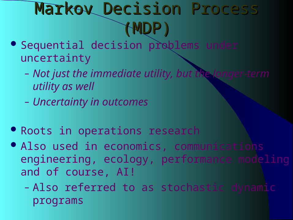
Markov Decision Process (MDP)Markov Decision Process (MDP)

Sequential decision problems under uncertainty– Not just the immediate utility, but the longer-term utility

as well– Uncertainty in outcomes

Roots in operations research Also used in economics, communications engineering,

ecology, performance modeling and of course, AI! – Also referred to as stochastic dynamic programs

Markov Decision Process (MDP)Markov Decision Process (MDP) Defined as a tuple: <S, A, P, R>

– S: State– A: Action– P: Transition function

Table P(s’| s, a), prob of s’ given action “a” in state “s”– R: Reward

R(s, a) = cost or reward of taking action a in state s

Choose a sequence of actions (not just one decision or one action)– Utility based on a sequence of decisions

Example: What SEQUENCE of actions Example: What SEQUENCE of actions should our agent take?should our agent take?

Reward

-1

Blocked

CELL

Reward

+1

Start1 2 3 4

1

2

3

0.8

0.10.1

• Each action costs –1/25• Agent can take action N, E, S, W• Faces uncertainty in every state

N

MDP Tuple: <S, A, P, R>MDP Tuple: <S, A, P, R> S: State of the agent on the grid (4,3)

– Note that cell denoted by (x,y) A: Actions of the agent, i.e., N, E, S, W

P: Transition function – Table P(s’| s, a), prob of s’ given action “a” in state “s”– E.g., P( (4,3) | (3,3), N) = 0.1– E.g., P((3, 2) | (3,3), N) = 0.8– (Robot movement, uncertainty of another agent’s actions,…)

R: Reward (more comments on the reward function later)– R( (3, 3), N) = -1/25– R (4,1) = +1

??Terminology??Terminology

• Before describing policies, lets go through some terminology

• Terminology useful throughout this set of lectures

•Policy: Complete mapping from states to actions

MDP Basics and TerminologyMDP Basics and Terminology

An agent must make a decision or control a probabilistic system

Goal is to choose a sequence of actions for optimality Defined as <S, A, P, R> MDP models:

– Finite horizon: Maximize the expected reward for the next n steps

– Infinite horizon: Maximize the expected discounted reward.

– Transition model: Maximize average expected reward per transition.

– Goal state: maximize expected reward (minimize expected cost) to some target state G.

???Reward Function???Reward Function According to chapter2, directly associated with state

– Denoted R(I)– Simplifies computations seen later in algorithms presented

Sometimes, reward is assumed associated with state,action– R(S, A)– We could also assume a mix of R(S,A) and R(S)

Sometimes, reward associated with state,action,destination-state– R(S,A,J)

– R(S,A) = R(S,A,J) * P(J | S, A)J

Markov AssumptionMarkov Assumption

Markov Assumption: Transition probabilities (and rewards) from any given state depend only on the state and not on previous history

Where you end up after action depends only on current state– After Russian Mathematician A. A. Markov (1856-1922)– (He did not come up with markov decision processes

however)– Transitions in state (1,2) do not depend on prior state (1,1)

or (1,2)

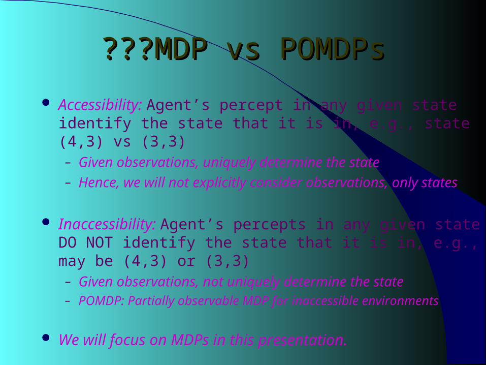
???MDP vs POMDPs???MDP vs POMDPs

Accessibility: Agent’s percept in any given state identify the state that it is in, e.g., state (4,3) vs (3,3)– Given observations, uniquely determine the state– Hence, we will not explicitly consider observations, only states

Inaccessibility: Agent’s percepts in any given state DO NOT identify the state that it is in, e.g., may be (4,3) or (3,3)– Given observations, not uniquely determine the state– POMDP: Partially observable MDP for inaccessible environments

We will focus on MDPs in this presentation.

MDP vs POMDP MDP vs POMDP

Agent

World

States

Actions

MDP

Agent

World

ObservationsActions

SE Pb

Stationary and Deterministic PoliciesStationary and Deterministic Policies Policy denoted by symbol

PolicyPolicy

Policy is like a plan, but not quite– Certainly, generated ahead of time, like a plan

Unlike traditional plans, it is not a sequence of actions that an agent must execute– If there are failures in execution, agent can continue to execute a

policy

Prescribes an action for all the states

Maximizes expected reward, rather than just reaching a goal state

MDP problemMDP problem

The MDP problem consists of:

– Finding the optimal control policy for all possible states;– Finding the sequence of optimal control functions for a specific

initial state– Finding the best control action(decision) for a specific state.

Non-Optimal Vs Optimal PolicyNon-Optimal Vs Optimal Policy

-1

+1

Start

1 2 3 4

1

2

3

• Choose Red policy or Yellow policy?• Choose Red policy or Blue policy?

Which is optimal (if any)?• Value iteration: One popular algorithm to determine optimal policy

Value Iteration: Key IdeaValue Iteration: Key Idea• Iterate: update utility of state “I” using old utility of

neighbor states “J”; given actions “A”– U t+1 (I) = max [R(I,A) + P(J|I,A)* U t (J)] A J

– P(J|I,A): Probability of J if A is taken in state I– max F(A) returns highest F(A)– Immediate reward & longer term reward taken into

account

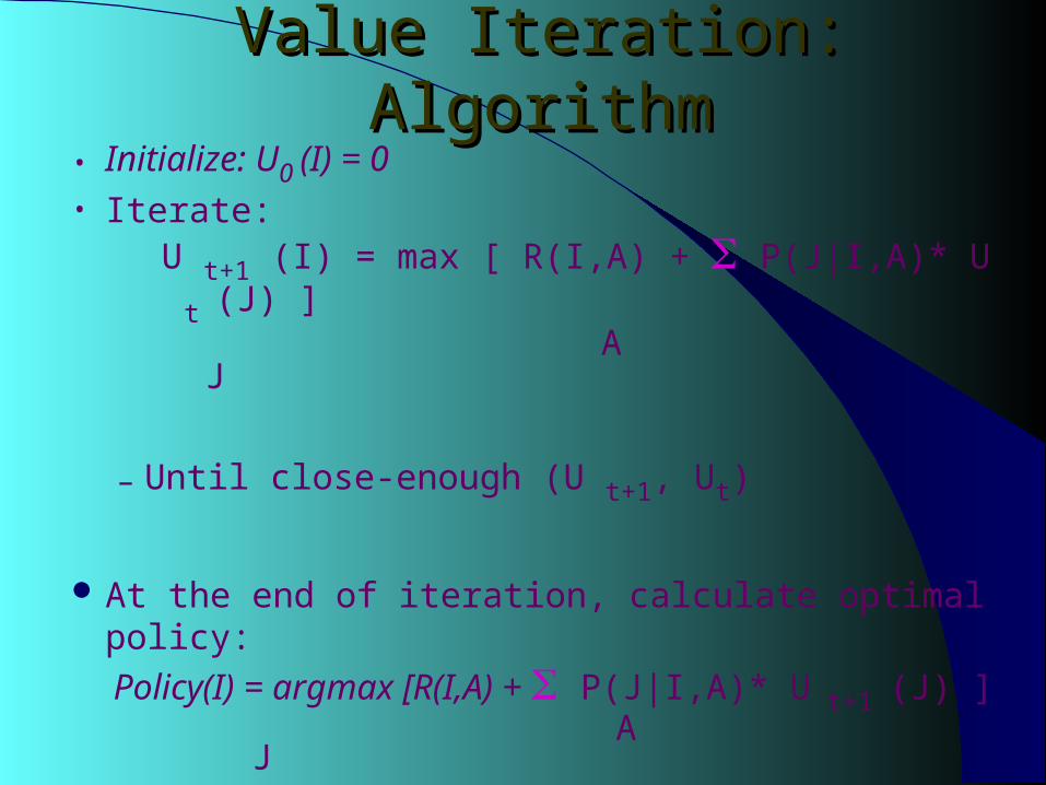
Value Iteration: AlgorithmValue Iteration: Algorithm• Initialize: U0 (I) = 0• Iterate:

U t+1 (I) = max [ R(I,A) + P(J|I,A)* U t (J) ] A J

– Until close-enough (U t+1, Ut)

At the end of iteration, calculate optimal policy:

Policy(I) = argmax [R(I,A) + P(J|I,A)* U t+1 (J) ] A J

Forward MethodForward Methodfor Solving MDPfor Solving MDP

Decision Tree

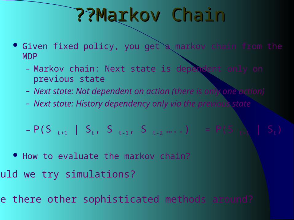
??Markov Chain??Markov Chain

Given fixed policy, you get a markov chain from the MDP– Markov chain: Next state is dependent only on previous state– Next state: Not dependent on action (there is only one action)– Next state: History dependency only via the previous state

– P(S t+1 | St, S t-1, S t-2 …..) = P(S t+1 | St)

How to evaluate the markov chain?

• Could we try simulations?

• Are there other sophisticated methods around?

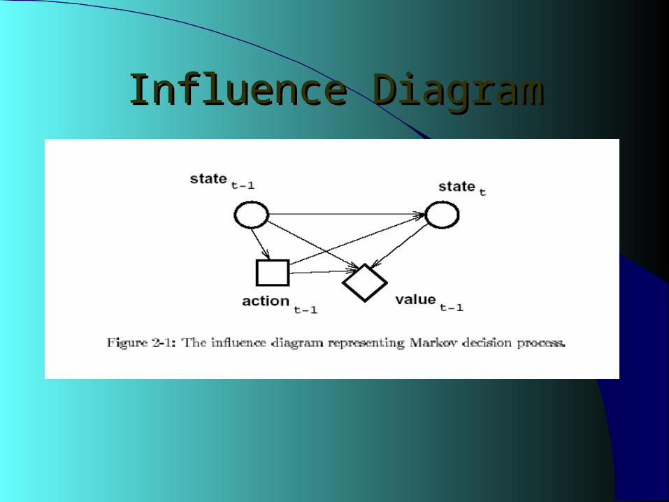
Influence DiagramInfluence Diagram

Expanded Influence DiagramExpanded Influence Diagram

Relation betweenRelation between time & steps-to-go time & steps-to-go

Decision TreeDecision Tree

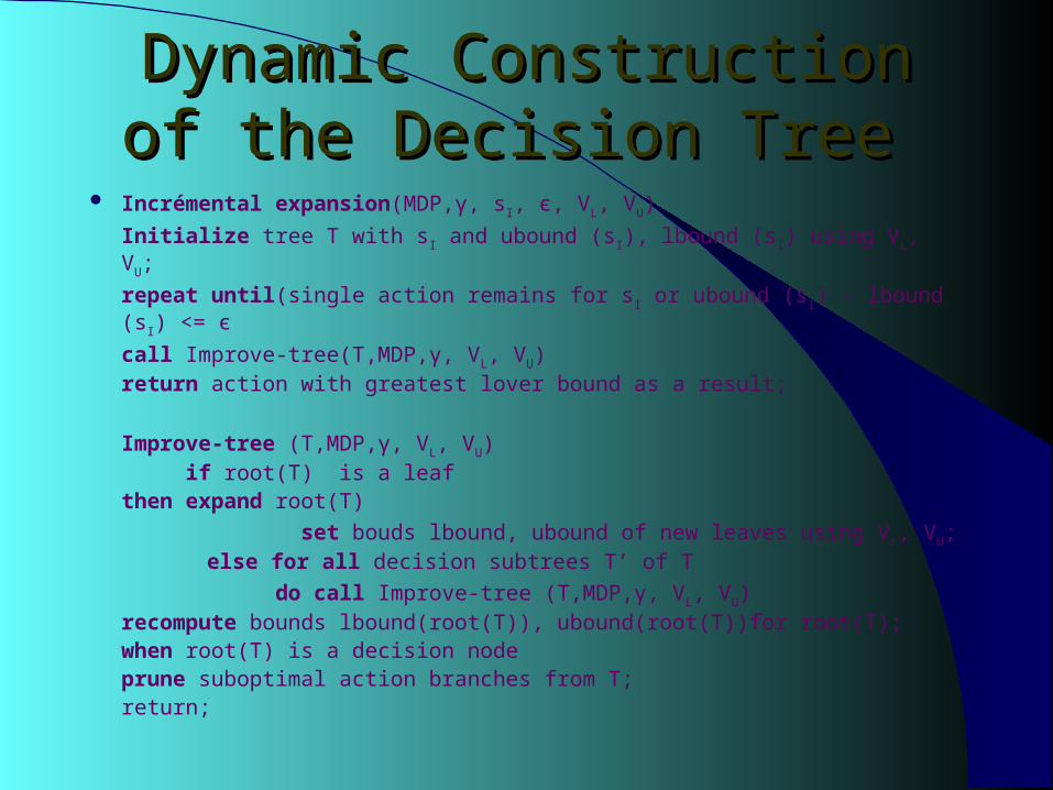
Dynamic ConstructionDynamic Constructionof the Decision Tree of the Decision Tree

Incrémental expansion(MDP,γ, sI, є, VL, VU)

Initialize tree T with sI and ubound (sI), lbound (sI) using VL, VU;

repeat until(single action remains for sI or ubound (sI) - lbound (sI) <= є

call Improve-tree(T,MDP,γ, VL, VU)return action with greatest lover bound as a result; 

Improve-tree (T,MDP,γ, VL, VU) if root(T) is a leaf

then expand root(T)

set bouds lbound, ubound of new leaves using VL, VU; else for all decision subtrees T’ of T

do call Improve-tree (T,MDP,γ, VL, VU)recompute bounds lbound(root(T)), ubound(root(T))for root(T);when root(T) is a decision node

prune suboptimal action branches from T;return;

Incremental expansion function:Basic Method for the Dynamic Construction of the Decision Tree

start

MDP, γ, SI, ε, VL, VU

OR SI)-bound(SI)

initialize leaf node of the partially built decision tree

return

call Improve-tree(T,MDP, γ, ε, VL, VU)

Terminate

Computer DecisionsComputer Decisionsusing Bound Iterationusing Bound Iteration

Incrémental expansion(MDP,γ, sI, є, VL, VU)

Initialize tree T with sI and ubound (sI), lbound (sI) using VL, VU;

repeat until(single action remains for sI or ubound (sI) - lbound (sI) <= є

call Improve-tree(T,MDP,γ, VL, VU)return action with greatest lover bound as a result; 

Improve-tree (T,MDP,γ, VL, VU) if root(T) is a leaf

then expand root(T)

set bouds lbound, ubound of new leaves using VL, VU; else for all decision subtrees T’ of T

do call Improve-tree (T,MDP,γ, VL, VU)recompute bounds lbound(root(T)), ubound(root(T))for root(T);when root(T) is a decision node

prune suboptimal action branches from T;return;

Incremental expansion function:Basic Method for the Dynamic Construction of the Decision Tree

start

MDP, γ, SI, ε, VL, VU

OR (SI)-bound(SI)

initialize leaf node of the partially built decision tree

return

call Improve-tree(T,MDP, γ, ε, VL, VU)

Terminate

Solving Large MDP problmesSolving Large MDP problmes

If You Want to Read MoreIf You Want to Read Moreon MDPson MDPs

If You Want to Read Moreon MDPs

Book:– Martin L. Puterman

Markov Decision Processes Wiley Series in Probability

– Available on Amazon.com