maxwell’s theory of electrodynamics - adam...
TRANSCRIPT

Maxwell’s Theory of Electrodynamics
From lectures given byYaroslav Kurylev
Edited, annotated and expanded byAdam Townsend & Giancarlo Grasso
19 May 2012

MATH3308 Maxwell’s Theory of Electrodynamics
Figure 1: Our Dear Leader and His Spirit Guide
2

Contents
1 Introduction to the Theory of Distributions 5
1.1 Introduction . . . . . . . . . . . . . . . . . . . . . . . . . . . . . . . . . 5
1.2 Definitions and notation . . . . . . . . . . . . . . . . . . . . . . . . . . 6
1.3 Functionals . . . . . . . . . . . . . . . . . . . . . . . . . . . . . . . . . 12
1.4 Distributions . . . . . . . . . . . . . . . . . . . . . . . . . . . . . . . . 14
1.5 Support of a Distribution . . . . . . . . . . . . . . . . . . . . . . . . . . 19
1.6 Differentiation of Distributions . . . . . . . . . . . . . . . . . . . . . . . 22
1.7 Convolution . . . . . . . . . . . . . . . . . . . . . . . . . . . . . . . . . 24
1.8 Density . . . . . . . . . . . . . . . . . . . . . . . . . . . . . . . . . . . 30
1.9 Integration of Distributions . . . . . . . . . . . . . . . . . . . . . . . . 37
1.10 The Laplace Operator and Green’s Function . . . . . . . . . . . . . . . 42
2 Electrostatics 47
2.1 Introduction to electrostatics . . . . . . . . . . . . . . . . . . . . . . . . 47
2.2 The fundamental equations of electrostatics . . . . . . . . . . . . . . . 48
2.3 Divergence theorem and Stokes’ theorem . . . . . . . . . . . . . . . . . 51
2.4 Finding E and Φ for different ρ . . . . . . . . . . . . . . . . . . . . . . 52
2.5 Dipoles . . . . . . . . . . . . . . . . . . . . . . . . . . . . . . . . . . . . 53
2.6 Conductors . . . . . . . . . . . . . . . . . . . . . . . . . . . . . . . . . 61
2.7 Boundary value problems of electrostatics . . . . . . . . . . . . . . . . 64
2.8 Dirichlet boundary value problems for Laplace’s equation . . . . . . . . 67
3 Magnetism 77
3.1 The laws for magnetostatics . . . . . . . . . . . . . . . . . . . . . . . . 77
3.2 The laws of magnetodynamics . . . . . . . . . . . . . . . . . . . . . . . 82
3.3 Maxwell’s equations . . . . . . . . . . . . . . . . . . . . . . . . . . . . . 86
3.4 Etude on differential forms . . . . . . . . . . . . . . . . . . . . . . . . . 87
4 Electromagnetic Waves 91
4.1 Electromagnetic energy . . . . . . . . . . . . . . . . . . . . . . . . . . . 92
4.2 Electromagnetic waves in an homogeneous isotropic medium . . . . . . 94
4.3 Plane waves . . . . . . . . . . . . . . . . . . . . . . . . . . . . . . . . . 95
4.4 Harmonic plane waves . . . . . . . . . . . . . . . . . . . . . . . . . . . 97
3

Editors’ note
This set of course notes was released initially in April 2011 for the University Col-lege London mathematics course MATH3308, Maxwell’s Theory of Electrodynam-ics, a ten-week course taught by Professor Yaroslav Kurylev between January andMarch 2011. The editors were members of this class. These notes were publishedto http://adamtownsend.com and if you wish to distribute these notes, please directpeople to the website in order to download the latest version: we expect to be makingsmall updates or error corrections sporadically. If you spot any errors, you can leave acomment on the website or send an email to the authors at [email protected] hope you enjoy the notes and find them useful!
AKT GWGLondon, April 2011
Acknowledgments
The editors would like to thank the following for their help in the production of thisset of course notes:
• Lisa for catapults and providing essential Russian to English translation;
• Kav for questions;
• The Permutation Boys (Jonathan, James and Charles) for permuting;
• Ewan for patiently being Ian;
• Prof. Kurylev for coffee and many, many invaluable life lessons.
We would also like to thank those who have offered corrections since the originalpublication.
4

Chapter 1
Introduction to the Theory ofDistributions
1.1 Introduction
James Clerk Maxwell (1831–1879), pictured on page 2, was a Scottish mathematicianand physicist who is attributed with formulating classical electromagnetic theory, unit-ing all previously unrelated observations, experiments and equations of electricity,magnetism and even optics into one consistent theory. Maxwell’s equations demon-strated that electricity, magnetism and even light are all manifestations of the samephenomenon, namely the electromagnetic field. By the end of the course we’ll havebuilt up the mathematical foundation that we need in order to understand this fully(more so than Maxwell himself!), and we’ll have derived and used Maxwell’s famousequations. Although they bear his name, like much of mathematics, his equations (inearlier forms) come from the work of other mathematicians, but they were broughttogether for the first time in his paper, On Physical Lines of Force, published between1861 and 1862∗.
The first chapter of this course is concerned with putting together a mathematicallysound foundation which we can build Maxwell’s theory of electrodynamics upon. Max-well’s theory introduces functions that don’t have derivatives in the classical sense,so we use a relatively new addition to analysis in order to understand this. Thisfoundation is the Theory of Distributions. Distributions (not related to probabilitydistributions) are the far-reaching generalisations of the notion of a function and theirtheory has become an indispensable tool in modern analysis, particularly in the theoryof partial differential equations. The theory as a whole was put forth by the French†
mathematician Laurent Schwartz in the late 1940s, however, its most important ideas(of so-called ‘weak solutions’) were introduced back in 1935 by the Soviet mathem-atician Sergei Sobolev. This course will cover only the very beginnings of this theory.
∗Paraphrased from Wikipedia†Honest!
5

MATH3308 Maxwell’s Theory of Electrodynamics
1.2 Definitions and notation
Let me start by reminding you of some definitions and notation:
Definition 1.1 A compact set K in a domain Ω, denoted K ⋐ Ω is a closed, boundedset.
Notation 1.2 C∞(Ω) is the set of continuous functions which can be differentiatedinfinitely many times in a domain Ω.
Notation 1.3 C0(Ω) is the set of continuous functions which are equal to 0 outsidesome compact K ⋐ Ω. That is to say, if f ∈ C0, ∀x /∈ K, f(x) = 0. This is known asthe set of continuous functions with compact support
Notation 1.4 C∞0 (Ω) is the set of continuous, infinitely differentiable functions withcompact support
Notation 1.5 We use Br(x0) to denote the closed ball of radius r centred at a pointx0 in our domain Ω: that is to say,
Br(x0) = x ∈ Ω : |x− x0| ≤ rwhere | · | is the norm of our domain. For this course we’ll always say that ourdomains are subsets of Rn, so we don’t need to worry about special types of norm:|v| is the standard (Euclidean) length of the vector v, which we work out in the usualPythagorean way.∗
Note: we’ll use the convention of writing vectors in boldface (e.g. v) from chapter 2onwards—the first chapter deals heavily in analysis and since we are being general inwhich domain we’re working in (R, R2 or R3), the distinction between one-dimensionalscalars and higher-dimensional vectors is unnecessary; most of our results hold in ndimensions, and excessive boldface would clutter the notes. As such we’ll use standarditalic (e.g. v) unless clarity demands it of us.
1.2.1 The du Bois-Reymond lemma and test functions
We start by proving a very useful lemma, first proved by the German mathematicianPaul du Bois-Reymond.
Lemma 1.6 Let Ω ⊂ Rn be an open domain (bounded or unbounded). Let f(x) ∈C(Ω). Assume that for any φ ∈ C∞0 (Ω),
∫
Ω
f(x)φ(x)dx = 0.
∗You may find that other authors use the notations B(x0, r), B(x0, r) or Bc(x0, r) (where the barand c denote ‘closed’).
6

Chapter 1. Introduction to the Theory of Distributions
Then f ≡ 0.
Proof: We’ll approach this using contradiction. Say we have x0 ∈ Ω such thatf(x0) > 0.
f ∈ C(Ω), i.e.
∀ ε > 0, ∃ δ > 0 s.t. |x− x0| < δ =⇒ |f(x)− f(x0)| < ε
Let ε = 12f(x0), i.e. there exists a ball of radius δ, Bδ(x0) such that f(x) > 1
2f(x0) for
all x ∈ Bδ(x0).
Choose φ from C∞0 such that:
1. φ(x) ≥ 0 for all x
2. φ(x) = 1 for x ∈ B δ2
(x0)
3. φ(x) = 0 for x /∈ Bδ(x0).
Then look at ∫
Ω
f(x)φ(x)dx =
∫
Bδ(x0)
f(x)φ(x)dx
since φ is zero outside of this ball. But∫
Bδ(x0)
f(x)φ(x)dx ≥∫
B δ2
(x0)
f(x)φ(x)dx
since all the f(x)φ(x) terms are positive. Then∫
B δ2
(x0)
f(x)φ(x)dx =
∫
B δ2
(x0)
f(x)dx
since φ(x) = 1 by condition 2 above. Then∫
B δ2
(x0)
f(x)dx ≥ 1
2f(x0) · Vol(B δ
2
(x0)) > 0
by our choice of ε above.
But our initial assumption was that∫
Ω
f(x)φ(x)dx = 0
which is a contradiction.
The crucial result underlining the proof of this lemma is the following:
7

MATH3308 Maxwell’s Theory of Electrodynamics
Proposition 1.7 Let K1 and K2 be two compacts in Rn such that K1 ⋐ K2. Thenthere exists φ ∈ C∞0 (Rn) such that
1. 0 ≤ φ(x) ≤ 1 on Rn;
2. φ(x) = 1 on K1;
3. φ(x) = 0 on Rn \K2.
K1
φ = 1
K2
Rn
φ = 0
Figure 1.1: Proposition 1.7 tells us this exists
We can take from the lemma a simple corollary:
Corollary 1.8 Let f, g ∈ C(Ω). Then if ∀φ ∈ C∞0 (Ω),∫
Ω
f(x)φ(x)dx =
∫
Ω
g(x)φ(x)dx
then f = g.
Proof: Subtracting one side from the other gives∫
Ω
f(x)φ(x)dx−∫
Ω
g(x)φ(x)dx = 0
∫
Ω
(f(x)− g(x))φ(x)dx = 0
Then f(x)− g(x) = 0 by Lemma 1.6, i.e. f(x) = g(x).
To understand the importance of this result, remember that normally to test whethertwo functions f and g are equal, we have to compare their values at all points x ∈ Ω.By the Du Bois-Reymond lemma, however, this is equivalent to the fact that integralsof f and g with all φ ∈ C∞0 (Ω) are equal. Thus, functions are uniquely characterised bytheir integral with C∞0 (Ω) functions. It is, of course, crucial that we look at the valuesof integrals of f with all C∞0 (Ω) functions, i.e. to test f with all C∞0 (Ω) functionswhich are, therefore, called test functions.
8

Chapter 1. Introduction to the Theory of Distributions
Definition 1.9 C∞0 (Ω) is called the space of test functions and is often denotedD(Ω)
1.2.2 Topological vector spaces and multi-indices
Definition 1.10 D(Ω) is a topological vector space, i.e.
1. It is a linear vector space, i.e. if f, g ∈ D(Ω) and λ, µ ∈ R,
h(x) = (λf + µg)(x) = λf(x) + µg(x) ∈ D(Ω) x ∈ Ω
and h(x) = 0 for x /∈ Kf ∪Kg, i.e. x not in the compact support of either.
2. There is a notion of convergence, i.e. there is a meaning to fk −−−→k→∞
f . This is
defined shortly.
For the next few definitions we need to introduce a further few convenient definitions:
Definition 1.11 A multi-index α is an n-dimensional vector, where n = dim(Ω),with non-negative integer components:
α = (α1, α2, . . . , αn), αi = 0, 1, . . . i = 1, . . . , n
Multi-indices are convenient when we want to write high-order partial derivatives,namely
∂αφ(x) =∂|α|φ
∂xα1
1 · · ·∂xαnn
, j = 1, . . . , n, |α| = α1 + · · ·+ αn.
1.2.3 Null set and support
Definition 1.12 The null set of a function f , N (f), is the maximal open set in Ωwhere f ≡ 0. In other words, x0 ∈ N (f) if it has a neighbourhood x0 ∈ U ⊂ Ω withf(x) = 0 when x ∈ U and if any other open set A holds this property, then A ⊂ N (f)
Definition 1.13 The support of a function f , supp(f) is the complement of N (f)in Ω, i.e.
supp(f) = Ω \ N (f)
Note that by this definition, supp(f) is always closed in Ω.
9

MATH3308 Maxwell’s Theory of Electrodynamics
Example 1.14 Let Ω = R and
f(x) =
0 if x ≤ 0x if x > 0
Then N (f) = (−∞, 0) and supp(f) = [0,∞).
f(x) 6
-x
Figure 1.2: Look, a picture of the function!
1.2.4 Convergence
Definition 1.15 A function φk converges to φ in D(Ω) if the following two conditionsare satisfied:
1. For any multi-index α and any x ∈ Ω,
∂αφp(x)→ ∂αφ(x), as p→∞
i.e. all derivatives converge
2. There is a compact K ⋐ Ω such that
supp(φp), supp(φ) ⊂ K, p = 1, 2, . . .
Problem 1.16 For any φ ∈ D(Ω) and any multi-index β, show that
∂βφ ∈ D(Ω)
Proof:N (∂βφ) ⊃ N (φ) =⇒ supp(∂βφ) ⊂ supp(φ) ⋐ Ω
10

Chapter 1. Introduction to the Theory of Distributions
supp φp supp φ
K
Ω
Figure 1.3: Definition 1.15(2) in picture form
Problem 1.17 If ζ ∈ C∞(Ω), then for any φ ∈ D(Ω), show
ψ = ζφ ∈ D(Ω)
Proof:
supp(ψ) ⊂ supp(φ) ⋐ Ω
Problem 1.18 Let φp → φ in D(Ω) and let β = (β1, . . . , βn) be some fixed multi-index. Show that
∂βφp → ∂βφ in D(Ω).
Solution This just follows from condition 1 of the definition of φp converging toφ. X
Problem 1.19 ∗ Let ζ ∈ C∞(Ω), i.e. ζ is an infinitely differentiable function in Ω.Show that, for φp → φ in D(Ω),
ζφp → ζφ in D(Ω).
Solution Want to show that if ψp = ζφp, ψ = ζφ, that
1. ∀β, ∂βψp → ∂βψ
2. ∃K s.t. supp(ψp), supp(ψ) ⊂ K
So let’s do it.
11

MATH3308 Maxwell’s Theory of Electrodynamics
1.
∂βψp = ∂β(ζφp)
=∑
γ:γ≤β
(βγ
)(∂β−γζ
)(∂γφp)
which is the sum of C∞ terms. So as p→∞, since φp → φ in D(Ω),
→∑
γ:γ≤β
(βγ
)(∂β−γζ
)(∂γφ)
= ∂β(ζφ).
2. N (ψ) ⊃ N (φ) =⇒ supp(ψ) ⊂ supp(φ) ⋐ Ω since φp → φ in D(Ω).N (ψp) ⊃ N (φp) =⇒ supp(ψp) ⊂ supp(φp) ⋐ Ω.
And so ∃K ⋐ Ω such that supp(ψ), supp(ψp) ∈ K.
X
Problem 1.20 If φp → φ, ψp → ψ in D(Ω) and λ, µ ∈ R, show that
λφp + µψp → λφ+ µψ in D(Ω)
Problem 1.21 If φp → φ, ψp → ψ in D(Ω) and λp → λ, µp → µ in R, show that
λpφp + µpψp → λφ+ µψ in D(Ω)
1.3 Functionals
Now we move on to functionals :
Definition 1.22 A function F : V → R, mapping from a vector space onto thereals, is called a functional.
Definition 1.23 A continuous, linear functional F has the properties,
1. Linearity:
F (λv + µw) = λF (v) + µF (w); v,w ∈ V ; λ, µ ∈ R (1.1)
2. Continuity:F (vp)→ F (v) as vp → v (1.2)
12

Chapter 1. Introduction to the Theory of Distributions
Problem 1.24 1. Let F be a linear functional on a topological vector space V .Show that F (0) = 0, where 0 is the zero vector in V .
2. Assume, in addition, that F satisfies
F (vp)→ 0, as vp → 0
Show that then F is continuous.
1.3.1 Dual space
Definition 1.25 The space of continuous linear functionals on V is called the dualspace to V and is denoteda by V ′.
The dual space is itself a topological vector space if, for λ, µ ∈ R and F,G ∈ V ′ wedefine λF + µG by
(λF + µG)(v) = λF (v) + µG(v), v ∈ V (1.3)
and Fp → F if, for any v ∈ V ,
Fp(v)→ F (v), as p→∞. (1.4)
Problem 1.26 Show that H = λF + µG defined by (1.3) is a continuous linearfunctional on V , i.e. H satisfies (1.1), (1.2).
Proof: We need to check that this object is linear and continuous:
1. Linearity:
(λF + µG)(αv + βw) = λF (αv + βw) + µG(αv + βw)
and each F,G are linear functionals, therefore
= λ(αF (v) + βF (w)) + µ(αG(v) + βG(w))
= α[λF (v) + µG(v)] + β[λF (w) + µG(w)]
= α(λF + µG)(v) + β(λF + µG)(w)
2. Continuity:
(λF + µG)(vp) =λF (vp) + µG(vp)
−−−→p→∞
λF (v) + µG(v)
=(λF + µG)(v)
†Other, if not most, authors denote the dual space to V by V ∗
13

MATH3308 Maxwell’s Theory of Electrodynamics
Problem 1.27 ∗ Show that if Fp → F and Gp → G, where Fp, F, Gp, G ∈ V ′, then
λFp + µGp → λF + µG.
Solution Again, just like above,
(λFp + µGp)(v) = λFp(v) + µGp(v)
and, by the information given in the question,
−−−→p→∞
λF (v) + µG(v)
= (λF + µG)(v)
X
Problem 1.28 If Fp → F , Gp → G, λp → λ, µp → µ, show that
λpFp + µpGp → λF + µG
Solution We want to show then that
(λpFp + µpGp)(v)→ (λF + µG)(v)
So here we go, quite succinctly.
(λpFp + µpGp)(v) = λpFp(v) + µpGp(v)
−−−→p→∞
λF (v) + µG(v)
= (λF + µG)(v)
X
Example 1.29 Let V = R2, the space of 2-dimensional vectors. Recall that vp → viff ‖vp − v‖ → 0. Then V ′ is actually V itself and we define, for w ∈ V ′ (which isagain just a 2-vector) and v ∈ V ,
w(v) = w · v = w1v1 + w2v2
i.e. the scalar product of w and v.
1.4 Distributions
Let us return to the topological vector space D(Ω) = C∞0 (Ω). Then it has a dual spaceof its functionals.
14

Chapter 1. Introduction to the Theory of Distributions
Definition 1.30 The topological vector space D′(Ω) of continuous linear functionalson D(Ω) is called the space of distributions on Ω.
Let me just remind you of a definition and result from real analysis (MATH7102):
Definition 1.31 We say that φp converges to φ (φp −−−→p→∞
φ) uniformly if:
∀ε > 0 ∃P (ε) s.t. p > P (ε) =⇒ |φp(x)− φ(x)| < ε ∀x ∈ Ω
Lemma 1.32 Let φp ∈ C(Ω) and φp(x) → φ(x) for any x ∈ Ω. Then for anycompact K ⋐ Ω, φp → φ uniformly.
What are some examples of distributions?
Proposition 1.33 Take any f ∈ C(Ω). For any φ ∈ D(Ω), consider
Ff (φ) =
∫
Ω
f(x)φ(x)dx.
Then Ff is a distribution (a continuous linear functional on D(Ω)) called a distributionassociated with the function f . That is to say, the integrals form a linear continuousfunctional in D(Ω).
Proof:
1. Linearity:
Ff(λφ+ µψ) =
∫
Ω
f(x) (λφ(x) + µψ(x)) dx
= λ
∫
Ω
f(x)φ(x)dx+ µ
∫
Ω
f(x)ψ(x)dx
= λFf(φ) + µFf(ψ) (1.5)
i.e Ff satisfies (1.1).
2. Continuity:
Let φp → φ in D(Ω).Then we’re told in definition 1.15 that for any multi-index α,
∂αφp(x)→ ∂αφ(x) x ∈ Ω
So take α = (0, . . . , 0), then obviously since ∂0φ = φ, we get
φp(x)→ φ(x), x ∈ Ω
=⇒ f(x)φp(x)→ f(x)φ(x)
But we can’t say that∫f(x)φp(x) dx→
∫f(x)φ(x) dx because this simply isn’t
true.
15

MATH3308 Maxwell’s Theory of Electrodynamics
Counterexample: Take the interval (0, 1) and
φp(x) =
p if x ∈ (0, 1
p)
0 if x ∈ [1p, 1)
Then ∀x ∈ (0, 1), φp(x)→ 0 but∫ 1
0φp(x)dx = 1.
We need the extra condition that φp → φ uniformly.
Recall that the definition of convergence (1.15) says that there is a compactK ⋐ Ω such that
supp(φp), supp(φ) ⊂ K, p = 1, 2, . . .
Then by Lemma 1.32 above, we have all we need and
Ff(φp) =
∫
K
f(x)φp(x)dx→∫
K
f(x)φ(x)dx = Ff(φ). (1.6)
This completes the proof.
So in summary, every f ∈ C(Ω) defines a distribution Ff ∈ D′(Ω), where
Ff(φ) =
∫
Ω
f(x)φ(x)dx
Moreover, the Du Bois-Reymond lemma says that to two different functions f1 andf2, we associate different Ff1 and Ff2 .
So we say that C is embedded in D′, C(Ω) ⊂ D′(Ω), and this embedding is continuous.
Previously we defined uniform convergence of a function, let us state what it meansfor a function to converge pointwise:
Definition 1.34 A function fp −−−→p→∞
f pointwise in C(Ω) if
fp(x)→ f(x) ∀x ∈ Ω
Problem 1.35 ∗ If fp, f ∈ C(Ω) and fp → f pointwise, show that
Ffp → Ff in D′(Ω)
Proof: Ffp → Ff in D′(Ω) means that
∀φ ∈ D′(Ω), Ffp(φ)→ Ff(φ) ⇐⇒∫
Ω
fp(x)φ(x)dx→∫
Ω
f(x)φ(x)dx
⇐⇒∫
K
fp(x)φ(x)dx→∫
K
f(x)φ(x)dx
16

Chapter 1. Introduction to the Theory of Distributions
where K = supp(φ).
Since fpφ→ fφ pointwise, and fpφ and fφ are continuous, then fpφ → fφ uniformlyin K.
1.4.1 Distributions of different forms
This leads us to the next question: are there any distributions F ∈ D′(Ω) which arenot of the form Ff for some f ∈ C(Ω)?
Definition 1.36 Let y ∈ Ω. Define the Dirac delta functional,
δy(φ) := φ(y). (1.7)
Problem 1.37 Show that the Dirac delta functional is a distribution.
Proof:
1. Linearity:
δy(λφ+ µψ) = (λφ+ µψ)(y)
= λφ(y) + µψ(y)
= λδy(φ) + µδy(ψ)
2. Continuity: if φp → φ in D, then, in particular, φp(y)→ φ(y), so that
δy(φp) = φp(y)→ φ(y) = δy(φ)
Problem 1.38 Show that there is no f ∈ C(Ω) such that δy = Ff .
Solution Without loss of generality, take y = 0. Assume δ = Ff with f ∈ C(Ω) andtake a function φε ∈ D(Ω) such that
0 ≤ φε(x) ≤ 1 in Ω
φε(x) = 1 in Bε
φε(x) = 0 outside B2ε
17
MATH3308 Maxwell’s Theory of Electrodynamics
δ(φε) = φε(0) = 1 so
1 = δ(φε) = Ff(φε) =
∣∣∣∣∣∣
∫
Ω
f(x)φε(x) dx
∣∣∣∣∣∣
=
∣∣∣∣∣∣
∫
B2ε
f(x)φε(x) dx
∣∣∣∣∣∣
≤∫
B2ε
|f(x)| |φε(x)| dx
≤∫
B2ε
|f(x)| dx
Let f ∈ C(Ω). Since f is continuous, it is bounded in any compact, i.e.
|f(x)| ≤ C in B1
(where we’ve picked the radius of the ball to be 1 fairly arbitrarily). Therefore
1 ≤ C
∫
B2ε
dx
= C · (vol. of ball in n-dim. case) · (2ε)n→ 0 as ε→ 0
which is a contradiction. X
Now for more examples of distributions:
Example 1.39 Let Ω = R3. Consider the plane, say x3 = a. Let h(x1, x2) be acontinuous function of two variables, i.e. h ∈ C(R2). Define
Fa,h(φ) =
∫h(x1, x2)φ(x1, x2, a) dx1 dx2,
i.e. the integral over the plane x3 = a:
=
∫
planex3=a
h(x)φ|R dA
Then Fa,h ∈ D′(R3) (we could denote this by hδa(x3)).
Example 1.40 More generally, let S ⊂ Ω ⊂ R3 be a surface and h a continuousfunction on S. Define
FS,h(φ) =
∫
S
hφ dAS,
where dAS is the area element on S, known as the surface integral from MATH1402.
18

Chapter 1. Introduction to the Theory of Distributions
Example 1.41 Let now, L be a curve in Ω ⊂ R2 or Ω ⊂ R3 and h be some continuousfunction on L. We define
FL,h(φ) =
∫
L
hφ dℓ
where dℓ is the length element on L.
Problem 1.42 Show that Fa,h ∈ D′(R3), as well as FS,h, FL,f ∈ D′(Ω).
1.5 Support of a Distribution
We know what supp(f) is when f ∈ C(Ω): this is the closure of the set of points wheref(x) 6= 0. This definition uses the values of the function at all points. Can we findsupp(f) looking only at
Ff(φ) =
∫
Ω
f(x)φ(x)dx?
To this end, observe that if supp(φ) ⊂ N (f), then
Ff(φ) = 0.
Moreover, by the Du Bois-Reymond lemma, if U ⊂ Ω is open and, for any φ ∈ D(Ω)with supp(φ) ⊂ U ,
Ff (φ) =
∫
Ω
f(x)φ(x)dx = 0,
then f = 0 in U , i.e. U ⊂ N (f). This makes it possible to find N (f) and, therefore,supp(f), looking only at Ff .
This also motivates the following definition:
Definition 1.43 Let F ∈ D′(Ω). We say that F = 0 in an open U ⊂ Ω (we candenote this F |U) if
F (φ) = 0, φ ∈ D(Ω), supp(φ) ⊂ U. (1.8)
This is a very natural definition: that, the distribution F is zero in U if, for whicheverfunction φ ∈ D = C∞0 we put into it, the result is zero so long as the support of φ (i.e.the non-zero bits) is contained entirely in U .
Definition 1.44 The null-set N (F ) is the largest open set U in Ω such that (1.8) isvalid when supp(φ) ⊂ U (i.e. the largest open set where F = 0).
19

MATH3308 Maxwell’s Theory of Electrodynamics
Definition 1.45 The support supp(F ) is the closed set
supp(F ) = Ω \ N (F ).
The consistency of this definition is based on the fact (which I shan’t prove) that
F = 0 in U1 and F = 0 in U2 =⇒ F = 0 in U1 ∪ U2. (1.9)
Problem 1.46 Show that supp(δy) = y
Proof: If supp(φ) ⊂ Ω \ y, then φ(y) = 0. Therefore,
δy(φ) = φ(y) = 0.
Thus(Ω \ y) ⊂ N (δy).
Now let’s assume that y ∈ N (δy). Then N (δy) = Ω since we’ve just added y to(Ω \ y), and
N (δy) = Ω ⇐⇒ δy(φ) = 0 ∀φ ∈ D(Ω).But Proposition 1.7 says that there exists φ ∈ D(Ω) such that φ(y) = 1. But thenδy(φ) = φ(y) = 1, which is clearly a contradiction.
Hence y /∈ N (δy).
Problem 1.47 Suppose S ⊂ Ω and h is a continuous function on S. Show thatsupp(FS,h) ⊂ S.
Proof:
FS,h(φ) =
∫
S
h(x)φ|S(x) dA
Look at the supports:Ω \ S ⊂ N (FS,h)
since F is integrating over an area S (if you take away S you’re left with nothing).Hence, taking complements,
S ⊃ supp(FS,h)
Actually, supp(FS,h) = S ∩ supp(h).
Problem 1.48 ∗ Show that supp(FL,h) ⊂ L.
20

Chapter 1. Introduction to the Theory of Distributions
Proof:
FL,h(φ) =
∫
L
h(x)φ|L(x) dℓ
Look at the supports:Ω \ L ⊂ N (FL,h)
since F is integrating over a line L (if you take away L you’re left with nothing).Hence, taking complements,
L ⊃ supp(FL,h)
1.5.1 Distributions with compact support (E ′)
The subclass of distributions with compact support is denoted by
E ′(Ω) ⊂ D′(Ω).
Definition 1.49 F ∈ E ′(Ω) if supp(F ) is compact in Ω.
The importance of E ′(Ω) is that we can unambiguously define F (ψ) for any ψ ∈ C∞(Ω)when F ∈ E ′(Ω).
Indeed, let supp(F ) ⊂ K1 ⊂ K2 ⋐ Ω, where K1 and K2 satisfy the conditions ofProposition 1.7.
Let
φ(x) ∈ D(Ω) =
1 if x ∈ K1
0 if x ∈ Ω \K2
(the existence of such φ is guaranteed by Proposition 1.7).
We now defineF (ψ) := F (φψ). (1.10)
Note that this definition is independent of the choice of φ satisfying
φ(x) = 1 x ∈ supp(F ).
Indeed, if φ is another function with this property, then
F (φψ)− F (φψ) = F ((φ− φ)ψ) = 0,
since supp(F ) ∩ supp((φ− φ)ψ) = ∅.
Definition 1.50 We say that Fp → F in E ′(Ω) if Fp → F in D′(Ω). That is tosay, Fp(φ) → F (φ) for any φ ∈ D(Ω) and there is a compact K ⋐ Ω such thatsupp(Fp), supp(F ) ⊂ K.
21

MATH3308 Maxwell’s Theory of Electrodynamics
1.6 Differentiation of Distributions
Take a function f ∈ C∞(Ω). Then, for any multi-index β, define
g := ∂βf =∂|β|f
∂xβ1
1 · · ·∂xβnn
Obviously g ∈ C∞(Ω) as well. So
Fg(φ) =
∫
Ω
g(x)φ(x) dx
=
∫
Ω
∂βf(x)φ(x) dx
= (−1)|β|∫
Ω
f(x) ∂βφ(x)︸ ︷︷ ︸∈D(Ω)
dx (1.11)
= (−1)|β|Ff (∂βφ) (1.12)
where line 1.11 has been achieved by integrating by parts |β| times. You can think ofthis process like repeating this:
[φ(x)∂β−1f(x)
]︸ ︷︷ ︸This disappears since
f, φ = 0 at the boundaries
−∫
Ω
∂φ(x) ∂β−1f(x) dx
Therefore:
Definition 1.51 For F ∈ D′(Ω) and a multi-index β, then ∂βF ∈ D′(Ω) is thedistribution of the form
∂βF (φ) = (−1)|β|F (∂βφ)and is called the β-derivative of the distribution F .
Let us just show that this definition is OK.
First, since φ has infinitely many derivatives, then ∂βφ also has infinitely many deriv-atives. Moreover, since φ = 0 on the open set N (φ), then (−1)|β|∂βφ = 0 on N (∂βφ),which is larger than N (φ) and
supp(∂βφ) ⊂ supp(φ).
This implies that supp(∂βφ) is a compact in Ω. Therefore, line 1.12 above is well-defined.
Now, to show that (1.12) is a distribution, we should prove the relations of linearity(1.5) and continuity (1.6).
22
Chapter 1. Introduction to the Theory of Distributions
1. Linearity:
∂βF (λ1φ1 + λ2φ2) = (−1)|β|F (∂β[λ1φ1 + λ2φ2])
= (−1)|β|F (λ1∂βφ1 + λ2∂βφ2)
= (−1)|β|λ1F (∂βφ1) + (−1)|β|λ2F (∂βφ2)
= λ1∂βF (φ1) + λ2∂
βF (φ2).
2. Continuity: by the definition of convergence, if φp → φ, then
∂βφp → ∂βφ
Thus,
∂βF (φp) = (−1)|β|F (∂βφp)→ (−1)|β|F (∂βφ) = ∂βF (φ).
Thus, for distributions associated with smooth functions, the derivatives of these dis-tributions are associated with the derivatives of the corresponding functions. Thisobservation shows that our definition 1.51 is a natural extension of the notion of dif-ferentiation from functions to distributions.
Problem 1.52 The Heaviside step function, Θ(x) or H(x), for x ∈ R, is given by
H(x) =
0 if x < 01 if x ≥ 0
.
Show that H ′ = δ, where H represents the distribution derived from the functionH(x).
Proof:
H ′(φ) = (−1)H(φ′)
= −∫ ∞
0
φ′(x) dx
= φ(0) [since φ(∞) = 0 because of compact support]
= δ(φ)
Problem 1.53 The sign (or signum) function, sgn(x), for x ∈ R is given by
−1 if x < 00 if x = 01 if x > 0
.
Show that sgn′ = 2δ.
23
MATH3308 Maxwell’s Theory of Electrodynamics
Proof:
sgn′(φ) = (−1) sgn(φ′)
= −∫ ∞
−∞sgn(x)φ′(x) dx
= −(∫ 0
−∞sgn(x)φ′(x) dx+
∫ ∞
0
sgn(x)φ′(x) dx
)
= −(−∫ 0
−∞φ′(x) dx+
∫ ∞
0
φ′(x) dx
)
= −(− [φ(x)]0−∞ + [φ(x)]∞0
)
= − (− (φ(0)− φ(−∞)) + (φ(∞)− φ(0)))= 2φ(0) [since φ(∞) = φ(−∞) = 0 because of compact support]
= 2δ(φ)
Problem 1.54 Show that, for any multi-index α and any y ∈ Ω,
∂αδy(φ) = (−1)|α|(∂αφ)(y).
Solution
∂αδy(φ) = (−1)|α|δy(∂αφ)= (−1)|α|(∂αφ)(y)
X
Note, in a matter unrelated to the problem above, that if F ∈ D′ is a distribution andψ ∈ C∞, then
(ψF )(φ) = F (ψφ), ψ ∈ D(Ω)
1.7 Convolution
An important operation acting on distributions is convolution. To define it, we start,as usual, with continuous functions.
24

Chapter 1. Introduction to the Theory of Distributions
Definition 1.55 Let
f ∈ C0(Rn)
g ∈ C(Rn)
i.e. f has compact support, supp(f) ⊂ K ⋐ Rn. Then define
h(x) = (f ∗ g)(x) :=∫
Rn
f(x− y)g(y) dy
=
∫
Rn
f(y)g(x− y)dy
= (g ∗ f)(x),
which is called the convolution of f and g. Clearly, f ∗ g ∈ C(Rn).
Consider the corresponding distribution Fh,
Fh(φ) = Ff∗g(φ) =
∫
Rn
∫
Rn
f(x− y)g(y)dy
φ(x)dx
=
∫
Rn
∫
Rn
f(x− y)φ(x)dx
g(y)dy
(z := x− y) =⇒ =
∫
Rn
∫
Rn
f(z)φ(z + y)dz
g(y)dy
(x := z) =⇒ =
∫
Rn
∫
Rn
f(x)φ(x+ y)dx
g(y)dy
(φy(x) := φ(x+ y)) =⇒ =
∫
Rn
∫
Rn
f(x)φy(x)dx
g(y)dy
=
∫
Rn
Ff (φy)︸ ︷︷ ︸
Φ(y)
g(y)dy
= Fg(Φ)
= Fg(Ff (φy))
Here, for any y ∈ Rn, we denoted by φy the translation of φ,
φy(x) = φ(x+ y).
Therefore,Ff∗g(φ) = Fg (Ff(φ
y)) . (1.13)
It turns out that formula (1.13) makes sense for any F ∈ E ′(Rn), G ∈ D′(Rn).
25

MATH3308 Maxwell’s Theory of Electrodynamics
Definition 1.56 For F ∈ E ′(Rn), G ∈ D′(Rn), we can define the convolution, H =F ∗G ∈ D′(Ω) by
(F ∗G)(φ) = G(F (φy)).
We will now show that this definition is (1) well-defined, (2) linear and (3) continuous.
1. Well-defined:
(a) Support:
Since F ∈ E ′(Rn),=⇒ supp(F ) ⋐ R
n
i.e. ∃b > 0 such that Rn \ Bb(0) ⊂ N (F ), where Bb(0) is a ball of radius bcentred at 0.
Since φ ∈ D(Rn),
=⇒ ∃a > 0 such that supp(φy) ⊂ Ba(y)
i.e. supp(φ) ⊂ Ba(0)
Thus if |y| > b+ a,supp(F ) ∩ supp(φy) = ∅
=⇒ F (φy) = 0
Denote Φ(y) = F (φy). Then supp(Φ) ⊂ Bb+a(0).
(b) Is Φ(y) ∈ C∞(Rn)?
We will show that Φ is infinitely differentiable by proving that
∂αΦ = F (∂αφy),
using induction on |α|.Assume
∂αΦ = F (∂αφy), |α| ≤ m
and let us show that
∂βΦ = F (∂βφy), |β| = m+ 1.
Let β = α+ ei, where
ei = (0, . . . , 0, 1, 0, . . . , 0)
with the 1 in the ith place.
By our inductive hypothesis,
∂i∂αΦ = ∂iF (∂
αφy)
but we need to prove that the right hand side exists. In order to do this,we need to show that:
ψs −−→s→0
ψ in D(Ω)
26

Chapter 1. Introduction to the Theory of Distributions
Where
ψs(y) =∂αφy+sei − ∂αφy
s, ψ(y) = ∂βφy
So we need, for any multi-index γ:
∂γψs −−→s→0
∂γψ
For |γ| = 0, we have:
ψs(y) =∂αφy+sei − ∂αφy
s=∂αφ(x+ y + sei)− ∂αφ(x+ y)
s−−→s→0
∂α+eiφ(x+ y)
=∂βφy = ψ(y)
Now, for an arbitrary multi-index γ, we want to show that:
∂γψs = ∂γ[∂αφ(x+ y + sei)− ∂αφ(x+ y)
s
]−−→s→0
∂γ+βφ(x+ y) = ∂γψ
Well,
∂γ+αφ(x+ y + sei)− ∂γ+αφ(x+ y)
s= ∂i∂
γ+αφ(x+ y)
= ∂γ+α+eiφ(x+ y)
= ∂γ+βφ(x+ y)
So ψs −−→s→0
ψ in D(Ω), which means that F (ψs) −−→s→0
F (ψ), now:
∂βΦ = ∂iF (∂αφy) = lim
s→0
F (∂αφy+sei)− F (∂αφy)
s
= lims→0
F
(∂αφy+sei − ∂αφy
s
)
= lims→0
F (ψs)
= F (ψ) = F (∂βφy)
So then, by induction, for any multi-index α
∂αF (φy) = F (∂αφy) (1.14)
Therefore F (φy) ∈ C∞(Rn). Thus G(F (φy)) is well defined.
2. Linearity: Clearly, the functional
φ 7→ G (F (φy))
is linear.
27

MATH3308 Maxwell’s Theory of Electrodynamics
3. Continuity: This is also a pain, but it’s the same type of pain.
Let φk → φ in D. We need
(F ∗G)φk → (F ∗G)(φ)
i.e.G(F (φy
k)) −−−→k→∞
G(F (φy)).
It is sufficient to show that
F (φyk) = Φk(y)→ Φ(y) = F (φy) in D.
So let’s check support and differentials
(a) Check support: Let us show that supp(Φk), supp(Φ) lie in the same ball.
As φk → φ in D, ∃a > 0 such that supp(φk), supp(φ) ⊂ Ba.
Then supp(Φk), supp(Φ) ⊂ Bb+a (where supp(F ) ⊂ Bb).
(b) Show ∂αΦk(y)→ ∂αΦ(y)
i.e. show F (∂αφyk)→ F (∂αφy)
Since φk → φ in D(Rn), this implies that φyk → φy in D(Rn).
Then by Proposition 1.7, ∂αφyk → ∂αφy in D(Ω) ∀α.
Therefore F (∂αφyk)→ F (∂αφy)
Congratulations!!! You did it!
Proposition 1.57 Convolution is a continuous map from E ′(Ω) × D′(Ω) to D′(Ω),i.e. if Fp → F in E ′(Ω) and Gp → G in D′(Ω), then
Fp ∗Gp → F ∗G.
We won’t prove this as it’s too difficult.
Problem 1.58 ∗ If Fp → F in E ′(Ω) and G ∈ D′(Ω), show that
Fp ∗G→ F ∗G
Solution
(Fp ∗G)(φ) = G(Fp(φy))
G is continuous, and Fp → F in E ′(Ω), so Fp(φy)→ F (φy), and hence
−−−→p→∞
G(F (φy))
= (F ∗G)(φ)
X
28

Chapter 1. Introduction to the Theory of Distributions
Lemma 1.59F ∗G = G ∗ F. (1.15)
Remark 1.60 We prove (1.15) later, although it’s obvious for distributions from thefunctions: if F = Ff , G = Fg,
G ∗ F = Fh h(x) =
∫g(x− y)f(y) dy
F ∗G = Fh h(x) =
∫f(x− y)g(y) dy
which are clearly equal.
Although the convolution of distribution is usually defined only for Ω = Rn, in somecases it may be defined for general Ω. In particular, when 0 ∈ Ω, F ∗ G is defined forF = ∂αδ, where α is arbitrary.
Problem 1.61 Show that(∂αδ) ∗G = ∂αG.
Solution
[(∂αδ) ∗G](φ) = G[(∂αδ)(φy)]
= G[(−1)|α|δ(∂αφy)]
= (−1)|α|G[δ(∂αφy)]
= (−1)|α|G[∂αφ]= (∂αG)(φ)
X
Now we will show that we can move about derivatives:
Proposition 1.62 Let F ∗G ∈ D′(Ω) be the convolution of two distributions. Then,for any multi-index α,
∂α(F ∗G) = (∂αF ) ∗G = F ∗ (∂αG).
Proof: By the definition of differentiation (definition 1.51),
∂α(F ∗G)(φ) = (−1)|α|(F ∗G)(∂αφ)= (−1)|α|G(F (∂αφy))
by the definition of convolution (definition 1.56).
To proceed, notice that
∂αφy(x) =∂αφ(x+ y)
∂xα=∂αφ(x+ y)
∂yα
29
MATH3308 Maxwell’s Theory of Electrodynamics
Therefore
F (∂αφy) = F
(∂αφy
∂yα
)
=∂α
∂yα(F (φy))
by equation 1.14. So, proceeding,
∂α(F ∗G)(φ) = (−1)|α|(F ∗G)(∂αx φ)= (−1)|α|G(F (∂αx φy))
= (−1)|α|G(F (∂αy φy))
= (−1)|α|G(∂αy F (φy))
= ∂αy G(F (φy))
= (F ∗ ∂αG)(φ)
Note the importance of which variable we differentiate with respect to. And sinceF ∗G = G ∗ F , swapping F and G holds.
Corollary 1.63
∂β+γ(F ∗G) = ∂β(F ) ∗ ∂γ(G)
1.8 Density
Now for a little notation
Notation 1.64
F : C(Ω) 7→ D′(Ω) F(f) = Ff
As we know F(C(Ω)) 6= D′(Ω). However, we have the following density result
Theorem 1.65
cl (F(C0(Ω))) = D′(Ω),i.e. for any F ∈ D′(Ω), Ω ⊂ Rn, there is a sequence fp ∈ D(Ω) such that
Ffp −−−→p→∞
F in D′(Ω) (1.16)
Sketch of proof: We will prove this theorem in 2 parts:
1. We will show that the distributions with compact support, E ′(Ω) are dense inthe space of all distributions D′(Ω), i.e. we show that cl(E ′(Ω)) = D′(Ω).
30

Chapter 1. Introduction to the Theory of Distributions
2. We will show that the space of distributions of compact support due to continu-ous functions with compact support is dense in the space of distributions withcompact support, i.e. we show that cl (F(C0(Ω))) = E ′(Ω). We will do this inthree steps:
(a) For F , a distribution with compact support, we will construct a sequenceof distributions converging to F in D′(Ω).
(b) Then we will show that in fact these distributions all have compact support,lying in the same compact, so that they converge to F in E ′(Ω).
(c) Finally we will show that they are in fact all distributions due to continuousfunctions with compact support.
Once we have proven these facts we see that F(C0(Ω)) is dense in E ′(Ω) which is, inturn, dense in D′(Ω). Recall, by the nature of the closure operation, this then meansthat cl(F(C0(Ω))) = D′(Ω). (Since D′(Ω) = cl(E ′(Ω)) = cl(cl(C0(Ω))) = cl(C0(Ω)) asthe closure of a closed set is itself).
1. We will show that any distribution can be approximated by distributions withcompact support, i.e.
∀F ∈ D′(Ω), ∃Fp ∈ E ′(Ω) s.t. Fp → F
First, let Kp, p = 1, 2, . . . , be a sequence of compacts exhausting Ω, i.e.
Kp ⋐ Ω, Kp ⊂ int(Kp+1),
∞⋃
p=1
Kp = Ω.
In fact we can define them as
Kp =
x ∈ Ω : |x| ≤ p, dist(x, ∂Ω) ≥ 1
p
Now let χp ∈ D(Ω) be functions with the properties described by Proposition1.7, where K1 = Kp and K2 = Kp+1, i.e.
χp(x) =
1 if x ∈ Kp
0 if x ∈ Ω \Kp+1
Let F ∈ D′(Ω), then define Fp by:
Fp = χpF
Fp(φ) = χpF (φ) = F (χpφ).
Note thatsupp(Fp) ⊂ Kp+1. (1.17)
Indeed, if φ ∈ D(Ω) and supp(φ) ∩Kp+1 = ∅, then
Fp(φ) = χpF (φ) = F (χpφ︸︷︷︸0
) = 0.
31

MATH3308 Maxwell’s Theory of Electrodynamics
Also, Fp → F . To prove this, we want to show that
F (χpφ) = Fp(φ) −−−→p→∞
F (φ) ∀φ ∈ D(Ω)
which clearly it does. Indeed, for large p, K ⊂ Kp
Proof:dist(K, ∂Ω) = d > 0
since K ⋐ Ω. As K is a compact, K ⊂ BR, for some radius R > 0.
Hence for p > max(R, 1d), K ⊂ Kp.
2. (a) Any distribution with compact support can be approximated by distribu-tions of functions with compact support, i.e.
∀F ∈ E ′(Ω), ∃fp ∈ D(Ω) s.t. Ffp → F ∈ E ′(Ω)
Let us introduce a function χ(x) ∈ D(Rn) such that
i. supp(χ) ⊂ B1(0)
ii. χ(x) =
1 if x ∈ B1/2(0)0 if x ∈ Ω \B1(0)
iii.
∫
Rn
χ(x)dx = 1
iv. χ = χ(|x|) (i.e. χ is a radial function)
The existence of such χ follows easily from proposition 1.7.
Now consider, for sufficiently small ε > 0, a function χε(x) ∈ D(Rn) suchthat
i. supp(χε) ⊂ Bε(0)
ii. χε(x) =
1 if x ∈ Bε/2(0)0 if x ∈ Ω \Bε(0)
iii.
∫
Rn
χε(x)dx = 1
iv. χε(x) =1
εnχ(xε
)
Now defineF ε := χε ∗ F ∈ E ′(Ω) (1.18)
then for φ ∈ D(Ω), by the definition of convolution,
F ε(φ) = (χε ∗ F )(φ) = F (χε(φy))
= Fχε(φy)
:=
∫
Rn
χε(x)φ(x+ y) dx ∈ D(Rn)
and we’ll show now that
χε(φy)→ φ(y) ∈ D(Ω).
32
Chapter 1. Introduction to the Theory of Distributions
First note that
χε(φy) =
∫
|x|≤ε
χε(x)φ(x+ y) dx
=
∫
|x|≤ε
χε(x) [φ(y) + φ(x+ y)− φ(y)] dx
= φ(y)
∫
|x|≤ε
χε(x) dx+
∫
|x|≤ε
χε(x) [φ(x+ y)− φ(y)] dx
= φ(y) +
∫
|x|≤ε
χε(x) [φ(x+ y)− φ(y)] dx
As
∫
|x|≤ε
χε(x) dx = 1.
So we can write
χε(φy) = φ(y) +
∫
|x|≤ε
χε(x)[φ(x+ y)− φ(y)] dx
Observe that
sup|x|≤ε|φ(x+ y)− φ(y)| −−→
ε→00 ∀y ∈ Ω
i.e. pointwise in Ω, which means that φ(x+ y)− φ(y) −−→ε→0
0 uniformly on
any K ⋐ Ω. Hence
ψǫ(y) = χε(φy) = φ(y) +
∫
|x|≤ε
χε(x) [φ(x+ y)− φ(y)]︸ ︷︷ ︸→0 ∀y∈Ω
dx
−−→ε→0
φ(y) uniformly on any compact
i.e.ψǫ(y) = χε(φy)→ φ(y) ∀y ∈ Ω
and uniformly on any compact.
And the same goes for the derivative. If we replace χε(φy) by ∂αχε(φy), weuse the same trick and
∂αχε(φy)→ ∂αφ(y) ∀y ∈ Ω,α
This means that χε(φy) = ψε → φ in E(Ω) = C∞(Ω).
So (χε ∗ F )(φ) = F (χε(φy)) −−→ε→0
F (φ) since F ∈ E ′(Ω) and χε(φy) → φ in
E(Ω)
So χε ∗ F → F in D′(Ω).
33

MATH3308 Maxwell’s Theory of Electrodynamics
(b) Now we show that χε ∗ F ∈ E ′(Ω), i.e. We show that χε ∗ F has compactsupport. First, we find supp(χε(φy)).
Suppose d(y, supp(φ)) > ε then d(x + y, supp(φ)) > 0 for |x| ≤ ε, whichmeans that x+ y /∈ supp(φ), so:
χε(φy) =
∫
|x|≤ε
χε(x)φ(x+ y) dx = 0 ∀y s.t. d(y, supp(φ)) > ε
So, supp(χε(φy)) ⊂ y : d(y, supp(φ)) ≤ ε, i.e. supp(χε(φy)) lies in anε-vicinity of supp(φ).
Now we claim that supp(χε ∗ F ) ⊂ x : d(x, supp(F )) ≤ ε = supp(F )ε, i.esupp(χε ∗ F ) lies in an ε-vicinity of supp(F ).
Let φ be such that:
supp(φ) ∩ supp(F )ε = ∅
Then:
d(supp(φ), supp(F )) > ε
i.e. the ε-vicinity of supp(φ) lies outside of supp(F ). Thus:
supp(χε(φy)) ∩ supp(F ) = ∅
So:
(χε ∗ F )(φ) = F (χε(φy)) = 0 ∀φ s.t. supp(φ) ∩ supp(F )ε = ∅
Which means that:
supp(χε ∗ F ) ⊂ supp(F )ε
Now take ε0 =12d(supp(F ), ∂Ω) so that supp(F )ε0 is compact in Ω. Then:
∀ε ≤ ε0 supp(χε ∗ F ) ⊂ supp(F )ε ⊂ supp(F )ε0 ⋐ Ω
So that supp(χε ∗ F ) ⋐ Ω which means that:
χε ∗ F ∈ E ′(Ω)
(c) Now we show that, for ε < 12d(supp(F ), ∂Ω), χε ∗ F ∈ C∞0 (Ω)
In other words, there are functions hε ∈ C∞0 (Ω) s.t. χε ∗ F = Fhε
34

Chapter 1. Introduction to the Theory of Distributions
We approach this problem as we always do; in order to construct hε we firstlook at the case when F = Ff , then:
(χε ∗ Ff )(φ) = Ff (χε(φy))
=
∫f(y)
(∫χε(x)φ(x+ y)dx
)dy
=
∫ (∫f(y)χε(z − y)φ(z)dz
)dy
︸ ︷︷ ︸z=x+y,dz=dx
=
∫ (∫f(y)χε(z − y)φ(z)dy
)dz
=
∫φ(z)
(∫χε(z − y)f(y)dy
)dz
= Fhε(φ)
Where: hε(z) =
∫f(y)χε(y − z)dy
= Ff (χε,−z)
Where we have denoted χε,−z(x) = χε(x − z). Now we generalise this tothe case when F is any distribution, by trying to show that:
If hε = F (χε,−z) ∈ C∞0 (Ω), then χε ∗ F = Fhε
Now observe that:
χε(φy) =
∫χε(x)φ(x+ y)dx =
∫χε(z − y)φ(z)dz
= limδ→0
∑
i
χε(zi − y)φ(zi)δn
:= limδ→0
Rεδ(y)
Also that:
∂αy χε(φy) = ∂αy
∫χε(z − y)φ(z)dz =
∫∂αy χ
ε(z − y)φ(z)dz
= limδ→0
∑
i
∂αy χε(zi − y)φ(zi)δn
= limδ→0
∂αy∑
i
χε(zi − y)φ(zi)δn
= limδ→0
∂αy Rεδ(y)
35
MATH3308 Maxwell’s Theory of Electrodynamics
Thus
χε(φy) = limδ→0
Rεδ in D(Ω)
=⇒ (χε ∗ F )(φ) = F (χε(φy))
= limδ→0
F (Rεδ)
= limδ→0
F
(∑
i
χε(zi − y)φ(zi)δn)
= limδ→0
(∑
i
(F (χε,−zi)
)φ(zi)δ
n
)
=
∫F (χε,−z)φ(z)dz
=
∫hε(z)φ(z)dz hε(z) = F (χε,−z) ∈ C∞0 (Ω)
= Fhε(φ)
These three parts prove that cl(F(C∞0 (Ω)) = E ′(Ω)
So we see that cl(F(C∞0 (Ω)) = D′(Ω) since cl(E ′(Ω)) = D′(Ω).
Problem 1.66 ∗ Prove that χε −−→ε→0
δ (where χε represents the distribution from
the function χε defined in part 2a above).
Solution
Fχε(φ) =
∫
R2
χε(x)φ(x) dx ∈ D(R2)
and since χε(x) = 0 outside of Bε,
=
∫
Bε
χε(x)φ(x) dx
=
∫
Bε
χε(x)φ(x) dx+ φ(0)− φ(0)
and since φ(0) = φ(0)∫Bεχε dx =
∫Bεχεφ(0) dx,
=
∫
Bε
χε(x) [φ(x)− φ(0)] dx+ φ(0)
and as ε→ 0, the integral → 0, leaving us with
→ φ(0)
Hence χε → δ. X
36
Chapter 1. Introduction to the Theory of Distributions
Now we return to a lemma from earlier:
Lemma 1.59F ∗G = G ∗ F. (1.15)
Proof: Let Ffp → F , where fp ∈ D(Ω) and Ggp → G, where gp ∈ C(Ω). We know,by remark 1.60, that:
Ffp ∗Ggp = Ggp ∗ Ffp
and that, by proposition 1.57,
Ffp ∗Ggp −−−→p→∞
F ∗G
so
F ∗G = limp→∞
(Ffp ∗Ggp) = limp→∞
(Ggp ∗ Ffp) = G ∗ F.
1.9 Integration of Distributions
We complete this section with the notion of integration of distributions with respectto some parameter τ = (τ1, . . . , τn) ∈ A ⊂ Rn. Let Fτ ∈ D′(Ω) be continuous withrespect to τ , i.e. Fτ → Fτ0
, in D′(Ω), when τ → τ 0. Recall that this means that,
Fτ (φ)→ Fτ0(φ), as τ → τ 0; φ ∈ D(Ω).
Then, if g ∈ C0(A), we define a distribution Gg ∈ D′(Ω) by
Gg =
∫
A
g(τ )Fτdτ .
Gg(φ) =
∫
A
g(τ )Fτ (φ)dτ . (1.19)
We can check that ifFτ = Ff(τ )
where f(τ ) = f(x, τ ) ∈ C(Ω×A)then
Gg = Fh
h(x) =
∫
A
g(τ )f(x, τ ) dτ .
37

MATH3308 Maxwell’s Theory of Electrodynamics
Anyway, now let’s consider A = Ω = Rn.
As a particular case, consider the operation of translation. As usual, we start withf ∈ C(Ω), which we then continue by 0 on the whole Rn. Let y ∈ Rn. By translationof f by y we understand the operation
Ty : f 7→ fy, fy(x) = f(x− y).
Let us consider the corresponding distribution TyFf = Ffy ,
TyFf(φ) =
∫
Ω
f(x− y)φ(x) dx
=
∫
Rn
f(x− y)φ(x) dx
=
∫
Rn
f(x)φ(x+ y) dx
= Ff (φy). (1.20)
We would like to use formula (1.20) to define the translation of distributions. However,in general, φy /∈ D(Ω) but just in C∞(Ω). Thus, assuming that F ∈ E ′(Ω) we find thefollowing definition
Definition 1.67 Let F ∈ E ′(Ω), y ∈ Rn. Then,
TyF (φ) = F (φy), φ ∈ D(Ω), (1.21)
and we continue it by 0 outside Ω.
There are a few different notations for translation, one of Prof. Kurylev’s favourites isTyF = F (· − y), which the editors wish he wouldn’t use because it sucks. Another isTyF = Fy.
Example 1.68Ty(δ) = δy
Proof:
(Tyδ)(φ) = δ(φy)
= φy(0)
= φ(y)
= δy(φ)
Observe that the operation of translation TyF is a distribution in D′(Rn), which de-pends continuously on y:
TyF → Ty0F as y → y0.
38

Chapter 1. Introduction to the Theory of Distributions
Is it true that
(Ty(F ))(φ) = F (φy) −→?
(Ty0F )(φ) = F (φy0)?
Yes it is because if y → y0,
φy = φ(x+ y)→ φ(x+ y0) = φy0 in D(Rn)
And clearly
∂αφ(x+ y) −−−→y→y0
∂αφ(x+ y0) ∀α ∀x ∈ Rn
since the supports lie in the same compact (see the compacts of φy and φy0 movingtowards each other as y → y0).
Thus, if g(y) ∈ C0(Rn), we can define using equation 1.19
Gg =
∫
Rn
g(y)(TyF ) dy
Gg(φ) =
∫
Rn
g(y)F (φy) dy
Problem 1.69 Show that Gg = Fg ∗ F
Problem 1.70 ∗ Let f(x) = 34(1 − x2) for |x| ≤ 1, f(x) = 0 for |x| > 1, x ∈ R.
Denote fn(x) = nf(nx), n = 1, 2, . . . and let Fn ∈ D′(R) be a distribution given by
Fn(φ) =
∫ ∞
−∞fn(x)φ(x) dx, φ ∈ C∞0 (R).
Show that Fn → δ0, as n→∞, in D′(R).
Solution
Fn(φ) =
∫ ∞
−∞fn(x)φ(x) dx
and because f(x) has compact support on [−1, 1], f(nx) has compact support on[− 1
n, 1n
], and fn(x) = nf(nx),
=
∫ 1/n
−1/nfn(x)φ(x) dx.
39
MATH3308 Maxwell’s Theory of Electrodynamics
Now, by the mean value theorem, since fn(x) does not change sign on[− 1
n, 1n
], there
exists a point x0 ∈(− 1
n, 1n
)such that
= φ(x0)
∫ 1/n
−1/nfn(x) dx
= φ(x0)
∫ 1/n
−1/nn3
4(1− x2n2) dx
= φ(x0)
[3n
4
(x− x3n2
3
)]1/n
−1/n
= φ(x0)
[3n
4
(1
n− n2
3n3
)+
3n
4
(1
n− n2
3n3
)]
= φ(x0)
[2 · 3n
4
(2
3n
)]
= φ(x0)
and since x0 ∈(− 1
n, 1n
), as n→∞, x0 → 0, so
Fn(φ)→ φ(0)
i.e.Fn → δ0
X
Problem 1.71 ∗ Let
gn(x) =
−3
2n3x if |x| < 1
n
0 if |x| ≥ 1n
.
Show that Gn → δ′0, as n→∞, in D′(R).
Solution Note that
gn(x) =d
dxfn(x)
using the definition of f from Problem 1.70
=d
dx
[3n
4
(1− n2x2
)]on |x| < 1
n
= −3n42n2x
= −32n3x on |x| < 1
n
and since Fn → δ0, we conclude that Gn → δ′0, so long as I can show that ∂Hn → ∂Hfor some distribution H . And I can do this by pointing out that
∂Hn(φ) = Hn(−∂φ)−−−→n→∞
H(−∂φ)= ∂H(φ)
40

Chapter 1. Introduction to the Theory of Distributions
since Hn = Fn and H = δ0. X
Problem 1.72 Let f ∈ C(Rn) satisfy
∫
Rn
f(x)dx = 1,
∫
Rn
|f(x)|dx <∞.
Letfp(x) = pnf(px), p = 1, 2, . . . .
Show that fp → δ, as p→∞, in D′(Rn). (here fp stands for the distribution Ffp)
Solution
Ffp(φ) = pn∫
Rn
f(px)φ(x) dx
Letting y = px, then dy = pn dx, since x is an n-dimensional vector
=
∫
Rn
f(y)φ
(y
p
)dy
=
∫
Rn
f(y)φ(0) dy +
∫
Rn
f(y)
[φ
(y
p
)− φ(0)
]
︸ ︷︷ ︸→0 pointwise
dy
= φ(0)
∫
Rn
f(y) dy
︸ ︷︷ ︸1 by definition
= φ(0)
Now, pointwise convergence is OK but we really want uniform convergence for rigour,i.e. we want to show
∀ε ∃P (ε) s.t. p > P (ε) =⇒
∣∣∣∣∣∣
∫
Rn
f(y)
[φ
(y
p
)− φ(0)
]dy
∣∣∣∣∣∣< ε
The trick we’ll employ is that ∫
Rn
=
∫
BA
+
∫
Rn\BA
Let’s deal with the area outside the ball of radius A first. Using part of the questionsetup, ∫
Rn
|f(x)|dx = C <∞ =⇒ ∀δ ∃A(δ) s.t.∫
Rn\BA
|f(x)|dx < δ
41
MATH3308 Maxwell’s Theory of Electrodynamics
So if we define
M = max |φ(y)|
and take
δ =ε
4M
then we have∫
Rn\BA
∣∣∣∣f(y)[φ
(y
p
)− φ(0)
]∣∣∣∣ dy ≤ 2M
∫
Rn\BA
|f(y)|dy
≤ ε
2
Now, inside the ball of radius A,∣∣∣∣y
p
∣∣∣∣ ≤A
p−−−→p→∞
0
which we can write analysis-style as∣∣∣∣φ(y
p
)− φ(0)
∣∣∣∣ ≤ε
2Cif p ≥ P (ε)
(picking ε2C
for use later!) Therefore
∫
BA
|f(y)|∣∣∣∣φ(y
p
)− φ(0)
∣∣∣∣ dy ≤ε
2C
∫
Rn
|f(y)|dy = ε
2
X
1.10 The Laplace Operator and Green’s Function
Let us have φα ∈ C∞(Ω) and F ∈ D′(Ω), and
DF =∑
|α|≤mφα(x)∂
αF.
Can we solve the equation DF = δy?
If we can, then we have a distribution Gy ∈ D′(Ω) which we call Green’s function.Typically Gy depends continuously on y.
Recall that the Laplacian, ∇2, in Rn is given by
∇2φ =n∑
i=1
∂2φ
∂x2i.
42

Chapter 1. Introduction to the Theory of Distributions
Definition 1.73 A function (or, more generally, a distribution), Φy ∈ D′(Rn) iscalled Green’s function (or a fundamental solution) for the Laplacian, ∇2, at the pointy ∈ Rn, if
−∇2Φy = δy.
In the study of electromagnetism, the most important case is n = 3 (and, sometimes,n = 1 or n = 2). So, let us look for Green’s function in R3.
Lemma 1.74 The function
Φy(x) =1
4π|x− y| (1.22)
is the fundamental solution for ∇2 in R3.
Before proving the lemma, let us make some remarks. The notation Φy(x) for theGreen’s function is typical in physics, in mathematics we tend to use Gy(x). Note alsothat this fundamental solution is a distribution associated with the function (1.22).Note that Φy(x) /∈ C(R3), as it has a singularity at x = y, however, Φy(x) ∈ L1
loc(R3).
Strictly speaking we should write, instead of Φy, FΦybut from now on we will identify
f as representing Ff and just write
f(φ) = Ff (φ).
Proof: We need to show that
− (∇2Φy)(φ) = δy(φ) = φ(y). (1.23)
By definition
(∇2Φy)(φ) = Φy(∇2φ)
=
∫
R3
∇2φ(x)
4π|x− y|dx.
Denote by Bε(y) a ball of radius ε centred at y and observe that
∫
R3
∇2φ(x)
4π|x− y|dx = limε→0
∫
R3\Bε(y)
∇2φ(x)
4π|x− y|dx. (1.24)
Since 14π|x−y| is smooth in R3 \ Bε(y) we can integrate by parts in the above integral.
Recall the second of Green’s identities from MATH1402,
∫
V
(g∇2f − f∇2g
)dV =
∫
S
(∂f
∂ng − f ∂g
∂n
)dS, (1.25)
where S is the surface surrounding V and n is the exterior unit normal to S.
43

MATH3308 Maxwell’s Theory of Electrodynamics
We take
V = R3 \Bε(y)
f = φ
g =1
4π|x− y| .
Note that since φ ∈ D(R3), we can integrate over the infinite domain R3 \Bε(y). Notealso that on the sphere Sε(y), the normal vector n exterior to V looks into Bε(y). Atlast, note that
∇2g = ∇2
(1
4π|x− y|
)= 0. (1.26)
So ∫
V
(g∇2f − f∇2g
)dV =
∫
S
(∂f
∂ng − f ∂g
∂n
)dS,
becomes
∫
R3\Bε(y)
∇2φ
4π|x− y|dV =
∫
Sε
(∂φ
∂n
(1
4π|x− y|
)− φ ∂
∂n
(1
4π|x− y|
))dS (1.27)
Now, plugging this into equation 1.24 gives us
limε→0
∫
R3\Bε(y)
∇2φ(x)
4π|x− y|dx = limε→0
∫
Sε
(∂φ
∂n
(1
4π|x− y|
)− φ ∂
∂n
(1
4π|x− y|
))dS
=1
4πlimε→0
∫
Sε
(∂φ
∂n
(1
|x− y|
)− φ ∂
∂n
(1
|x− y|
))dS
Now recall that y is fixed—this is really important because it means we can do thefollowing substitutions
z := x− yThen convert to spherical coordinates
(z = ρ, θ, ϕ)
So φ(x) becomes a function of φ(y + ρω), where ω is a unit vector made up of θ andϕ. In fact,
ω = (sin θ cosϕ, sin θ sinϕ, cos θ)
Observe that∂
∂n= − ∂
∂ρ
Giving us1
4πlimε→0
∫
ρ=ε
(−∂φ∂ρ
(1
ρ
)+ φ
∂
∂ρ
(1
ρ
))dS
44

Chapter 1. Introduction to the Theory of Distributions
=1
4πlimε→0
∫
ρ=ε
(−∂φ∂ρ
(1
ε
)− φ 1
ε2
)dS
and dS = ε2 sin θ dθ dϕ which gives us that
(∇2Φy)(φ) = −1
4πlimε→0
∫
ρ=ε
(∂φ
∂ρ
1
ε+ φ
1
ε2
)ε2 sin θ dθ dϕ
and of course
∫
ρ=ε
=
∫∫
0≤θ≤π0≤ϕ≤2π
.
Now note that ∫∫∂φ
∂ρ
1
εε2 sin θ dθ dϕ −−→
ε→00
since ∂φ∂ρ
is bounded, and from what’s left,
− 1
4π
∫∫
θ,ϕ
φ(y + εω) sin θ dθ dϕ −−→ε→0− 1
4πφ(y)
∫∫
θ,ϕ
sin θ dθ dϕ
︸ ︷︷ ︸vol. of sphere
of radius 1 = 4π
= −φ(y).
So we have shown that
−∇2
(1
4π|x− y|
)= δy.
We want to let y = 0:
−∇2
(1
4π|x|
)= δ0?
Well,
−∇2
(Ty
1
4π|x|
)= Tyδ0,
and noting that Ty δα = δα Ty,
Ty
(−∇2 1
4π|x|
)= Tyδ0 = δy,
So it’s sufficient to prove that
−∇2
(1
4π|x|
)= δ0
and use commutativity to solve
−∇2
(1
4π|x− y|
)= δy
45

MATH3308 Maxwell’s Theory of Electrodynamics
1.10.1 Motivation
Why is knowledge of Green’s function such a useful thing?
Say we want to solve a differential equation with constant coefficients. Let cα beconstants and D be the differential operator:
D =∑
|α|≤mcα∂
α.
Suppose we wish to solve the differential equation:
DF = H
where H is a known function (or distribution) and F is our unknown. Now supposewe know G such that DG = δ, i.e. we know the Green’s function for our differentialoperator D. Now construct F = G ∗H so that:
DF = D(G ∗H)
=∑
|α|≤mcα∂
α(G ∗H).
By Proposition 1.62 and linearity
=
∑
|α|≤mcα∂
αG
∗H
= δ ∗H= H.
So we see that knowledge of the Green’s function for a differential operator, allows usto solve a differential equation with any right hand side, by use of the comparativelysimple operation of convolution.
For example if you ever wanted to solve −∇2F = g in Ω ⊂ R3, then
F =1
4π|x| ∗ g.
Observe that if g ∈ C0(R3),
F (x) =1
4π
∫
R3
g(y)
|x− y|dy.
46
Chapter 2
Electrostatics
Now finally we can apply this mathematics. In this chapter we apply it to electrostaticsand in the following chapter, we’ll apply it to magnetism (which is very similar), andin doing so, derive Maxwell’s famous equations.
2.1 Introduction to electrostatics
2.1.1 Coulomb’s law
F1←2
x1
q1
F2←1*x2
q2
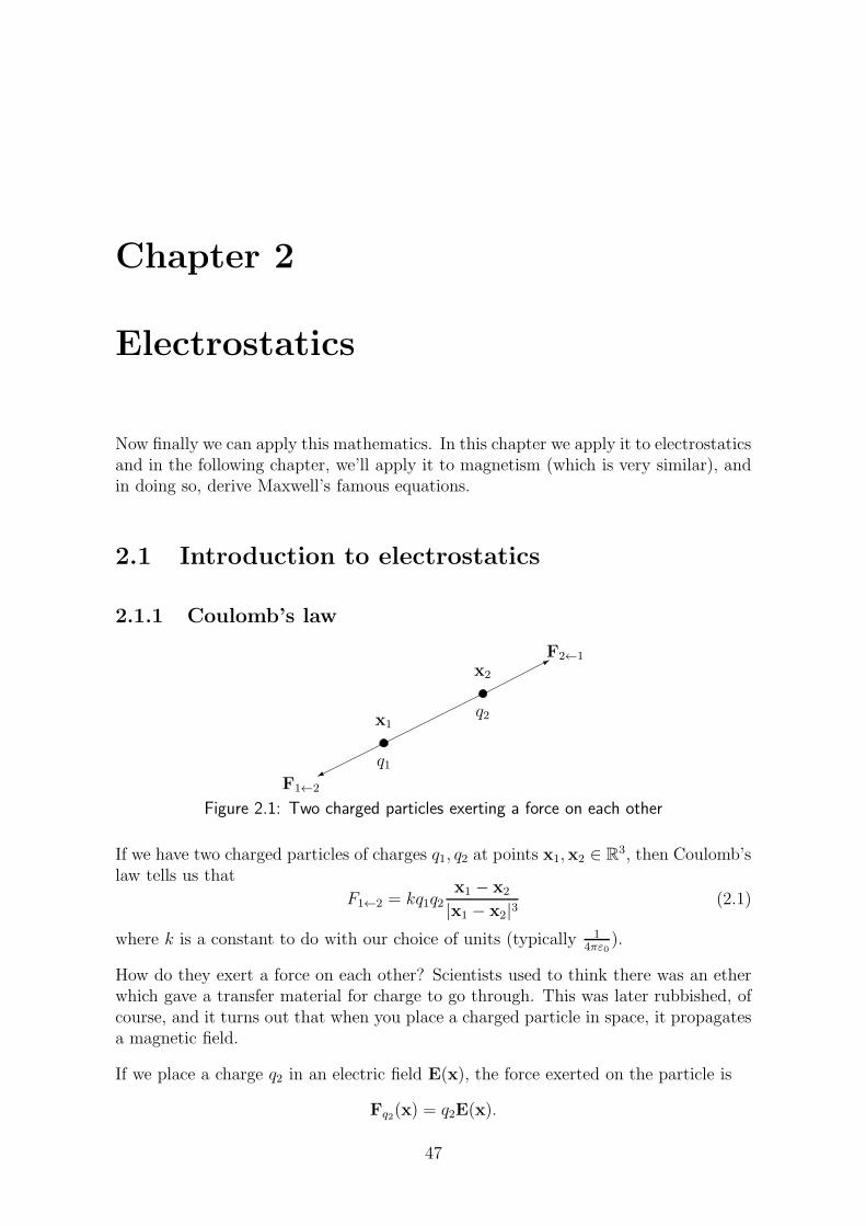
Figure 2.1: Two charged particles exerting a force on each other
If we have two charged particles of charges q1, q2 at points x1,x2 ∈ R3, then Coulomb’slaw tells us that
F1←2 = kq1q2x1 − x2
|x1 − x2|3(2.1)
where k is a constant to do with our choice of units (typically 14πε0
).
How do they exert a force on each other? Scientists used to think there was an etherwhich gave a transfer material for charge to go through. This was later rubbished, ofcourse, and it turns out that when you place a charged particle in space, it propagatesa magnetic field.
If we place a charge q2 in an electric field E(x), the force exerted on the particle is
Fq2(x) = q2E(x).
47
MATH3308 Maxwell’s Theory of Electrodynamics
Combining this with Coulomb’s law (2.1) above,
E(x) = kq1x1 − x2
|x1 − x2|3= kq1
(x1 − x2)
|x1 − x2|2
Electric fields add linearly.
2.1.2 Electric potential
If we have an electric field E, then we define the (scalar) electric potential Φ by
E(x) = −∇Φ(x)
(note that ∇×E = 0 and the domain is simply connected, so by what we learnt inMATH1402, E has a potential Φ.)
Obviously Φ is defined up to a constant, so it has no physical meaning, but thedifference of potentials does, of course.
So, taking a path ℓ between our two charges at x1 and x2, at any point x along thepath,
F(x) = qE(x).
The work done then getting from x to x+ δx is then dW = F(x) · dx, so
Work =W =
∫
ℓ
F(x) · dx
= q
∫
ℓ
E(x) · dx
= −q∫
ℓ
∇Φ(x) · dx
= −q [Φ(x2)− Φ(x1)]
= q [Φ(x1)− Φ(x2)]
The convention is that Φ = 0 at infinity.
2.2 The fundamental equations of electrostatics
We are now going to derive the fundamental equations of electrostatics, first in the caseof discrete point charges, and second in the case of a continuous charge distribution.
48

Chapter 2. Electrostatics
2.2.1 The discrete case
Definition 2.1 If we have a group of electric charges qi at positions yi, for i =1, . . . , p, then we say that the electric potential at the point x is
Φt(x) =
p∑
i=1
qi4πε0|x− yi|
(the t is for total!)
Definition 2.2 The electric field created by these charges is defined as
Et(x) = −∇Φt(x)
Definition 2.3 The charge density distribution created by these charges is definedas
ρ =
p∑
i=1
qiδyi
Lemma 2.4 If Φ is Green’s function and ρ is the discrete distribution as describedabove, then the electrostatic potential due to the distribution ρ of charges is
Φt = Φ ∗ ρε0
Proof:
Φ ∗ ρε0
=1
4π|x| ∗1
ε0
p∑
i=1
qiδyi
=1
ε0
p∑
i=1
(1
4π|x| ∗ qiδyi
)
︸ ︷︷ ︸What is this?
Recall that, for a distribution H ,
(δz ∗H)(φ) := H(δzφy)
= H(φy(z))
= H(φz) (since φy(z) = φz(y))
= (TzH)(φ)
so δz ∗H = TzH .
So1
4π|x| ∗ qiδyi=
qi4π|x− yi|
49

MATH3308 Maxwell’s Theory of Electrodynamics
and we getp∑
i=1
qi4πε0|x− yi|
= Φt(x)
2.2.2 The continuous case
Now we are given a distribution ρ ∈ E ′(R3). So what is Φρ, the electrostatic potentialdue to ρ?
Well, we want to usep∑
i=1
qi4πε0|x− yi|
but we want to make it continuous.
So consider that inside a small cube centred at xi in R3, the approximate charge is
qi = ρ(xi) δx δy δz.
Now take the limit as δx, δy, δz → 0.
limδxδyδz
→0
∑
i
ρ(xi) δx δy δz
4πε0|x− xi|=
1
4πε0
∫
R3
ρ(y)
|x− y|dy
=1
4π|x| ∗ρ
ε0
= Φ ∗ ρε0
= Φρ
So we get the same result as we did in the discrete case in Lemma 2.4, i.e.
Φρ = Φ ∗ ρε0
2.2.3 The equations
Take the Laplacian of our potential distribution Φρ:
−∇2Φρ = −∇2Φ ∗ ρε0
(by definition of Φ) = δ ∗ ρε0
=ρ
ε0
50

Chapter 2. Electrostatics
And recall that the definition of the electric field due to a particle distribution ρ is
Eρ = −∇Φρ
which gives us. . .
Definition 2.5 The fundamental equations of electrostatics are
1. ∇ · Eρ =ρ
ε0(Gauss’ law in differential form)
2. ∇× Eρ = 0
2.3 Divergence theorem and Stokes’ theorem
Problem 2.6 If F ∈ D′(Ω), where Ω ⊂ R3, then
(∂F
∂x,∂F
∂y,∂F
∂z
)= ∇F ∈ D′(Ω)3.
Show that∇×∇F = 0 and ∇ · (∇F ) = ∇2F
Taking the fundamental equations of electrostatics, let us put these into the divergencetheorem from MATH1402, for a domain V with boundary S:
∫
S
Eρ · n dS =
∫
V
∇ ·Eρ dV
But ∇ · Eρ = ρε0
=⇒
=1
ε0
∫
V
ρ dV =Q(V )
ε0(Gauss’ law in integral form)
where Q(V ) is the total charge in V . This is known as Gauss’ law in integral form.
Now what about putting Eρ into Stokes’ law? Recall that Stokes’ law, for some vectorF, is ∫
S
(∇× F) · n dS =
∮
C
F · dr
Substituting F = Eρ gives us
0 =
∫
S
(∇× Eρ)︸ ︷︷ ︸0
·n dS =
∮
C
Eρ · dr
but remember that Stokes’ law is only valid for simply connected domains.
51
MATH3308 Maxwell’s Theory of Electrodynamics
2.4 Finding E and Φ for different ρ
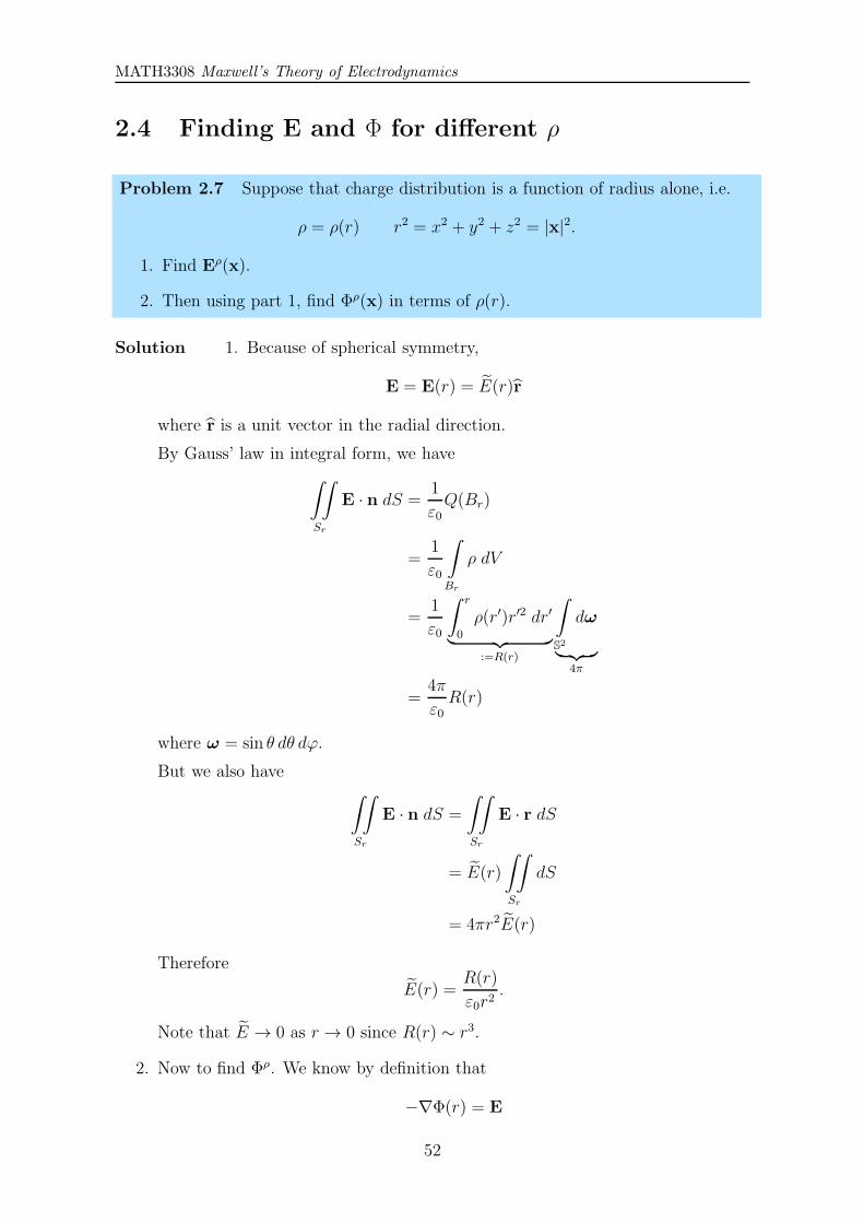
Problem 2.7 Suppose that charge distribution is a function of radius alone, i.e.
ρ = ρ(r) r2 = x2 + y2 + z2 = |x|2.
1. Find Eρ(x).
2. Then using part 1, find Φρ(x) in terms of ρ(r).
Solution 1. Because of spherical symmetry,
E = E(r) = E(r)r
where r is a unit vector in the radial direction.
By Gauss’ law in integral form, we have
∫∫
Sr
E · n dS =1
ε0Q(Br)
=1
ε0
∫
Br
ρ dV
=1
ε0
∫ r
0
ρ(r′)r′2 dr′
︸ ︷︷ ︸:=R(r)
∫
S2
dω
︸ ︷︷ ︸4π
=4π
ε0R(r)
where ω = sin θ dθ dϕ.
But we also have∫∫
Sr
E · n dS =
∫∫
Sr
E · r dS
= E(r)
∫∫
Sr
dS
= 4πr2E(r)
Therefore
E(r) =R(r)
ε0r2.
Note that E → 0 as r → 0 since R(r) ∼ r3.
2. Now to find Φρ. We know by definition that
−∇Φ(r) = E
52
Chapter 2. Electrostatics
Therefore, setting up Φ so that it is 0 at ∞,
Φ(r) = −∫ r
∞E(r′) dr′
=
∫ ∞
r
E(r′) dr′
=
∫ ∞
r
R(r′)
r′2dr′
We could be done at this point but it would be nice to integrate by parts sinceR itself is an integral. So, letting our ‘first’ be R(r) and our ‘second’ be 1/r2,
=
[R(r)
−1r
]∞
r
+
∫ ∞
r
R′(r′)1
r′dr′
=R(r)
r+
∫ ∞
r
ρ(r′)r′ dr′
X
Problem 2.8 ∗ Let ρ = ρ(r) in cylindrical coordinates (r, ϕ, z), i.e. r2 = x2 + y2.Find Eρ (using Gauss’ law).
Solution By symmetry, Eρ = E(r) = E(r)r, so
∇ · Eρ = ∇ · E(r)r
=1
r
d
dr
(rE(r)
)
=ρ
ε0
And so
E(r)− E(0)︸︷︷︸0
=1
rε0
∫ r
0
rρ(r) dr
=⇒ E(r) =1
rε0
∫ r
0
rρ(r) dr
and Eρ = E(r)r. X
2.5 Dipoles
We now introduce the idea of dipoles.
53
MATH3308 Maxwell’s Theory of Electrodynamics
Definition 2.9 If we have a charge distribution
ρ = p · ∇yδy = −p · ∇xδy p = pu
where u is a unit vector, then p · ∇δy is called the dipole of size p in the direction uat the point y.
Recall for maths’ sake that
p · ∇δy = p
(∂δy∂x
u1 +∂δy∂y
u2 +∂δy∂z
u3
)
= p∂δy∂u
Consider placing a charge psat the point y+ su, and a charge −p
sat the point y. This
is, physically, a dipole.
Then the electrostatic potential Φs = Φsp,y due to the two point charges
(psδy+su −
p
sδy
)
is
Φs =p
sε0
[1
4π|x− (y + su)| −1
4π|x− y|
]
Now take s→ 0:
lims→0
Φs(x) =p
ε0
∂
∂uyΦy(x)
= − p
ε0
∂
∂uxΦy(x)
Now in order to find Φdp,y, we first look at:
∇(
1
4π|x|
)
Taking each component of ∇ in turn:
∂
∂x
(1√
x2 + y2 + z2
)= −1
2· 2x · 1
(x2 + y2 + z2)3/2
= − x
|x|3
∂
∂y
(1√
x2 + y2 + z2
)= − y
|x|3
∂
∂z
(1√
x2 + y2 + z2
)= − z
|x|3
54
Chapter 2. Electrostatics
hence
∇(
1
4π|x|
)= − x
4π|x|3
But we know that for a dipole (d), of size p in direction u sitting on the point y,
Φdp,y =
1
ε0Φ ∗ (p · ∇yδy)
=1
ε0Φ ∗ (−p · ∇xδy)
= − 1
ε0p · ∇x(Φ ∗ δy)
= − 1
ε0(p · ∇Φ) ∗ δy
= − 1
ε0
(p · ∇
(1
4π|x|
))∗ δy
= − 1
ε0
(p ·(− x
4π|x|3))∗ δy
=1
4πε0
(p ·(
x
|x|3))∗ δy
=1
4πε0
p · (x− y)
|x− y|3
Since convolution with δy is the same as translation by −y
And so we get:
Definition 2.10 The potential of a dipole of size p in the direction u at a point y is
Φdp,y =
1
4πε0
p · (x− y)
|x− y|3
Now to find the corresponding electric field. Edp,y.
We know
Edp,y = −∇Φd
p,y
so let’s work it out.
Let y = 0 for ease. Then
Φdp,0 =
1
4πε0
(p1x1 + p2x2 + p3x3)
|x|3
55

MATH3308 Maxwell’s Theory of Electrodynamics
and working out Edp,0 component-wise, we get
Edp,y = −∇Φd
p,y
so∂Φd
p,0
∂x1= − 1
4πε0
(p1|x|3 −
3p1x21
|x|5).
Continuing this process we end up with
Edp,0 =
1
4πε0
(3(p · x)x− p
|x|3)
2.5.1 Jumps
Recall that for a surface S and h ∈ C0(S),
Fh,S(φ) =
∫
S
h(x)φ(x) dSx
We want to find, for the h-surface charge distribution, Φh,S and Eh,S.
Lemma 2.11
Φh,S(x) :=1
ε0Φ ∗ Fh,S =
1
4πε0
∫
S
h(y)
|x− y|dSy
Proof: We have
Φh,S(φ) =1
ε0Φ ∗ Fh,S(φ
y)
Fh,S(φy) =
∫
S
h(x)φ(x+ y)dSx ∈ D(R3)
(where y is fixed in dSx). Therefore
Φh,S(φ) =1
4πε0
∫
R3
1
|y|
∫
S
h(x)φ(x + y)dSx
dy
=1
4πε0
∫
S
h(x)
∫
R3
φ(x+ y)
|y| dy
dSx
=1
4πε0
∫
S
h(x)
∫
R3
φ(z)
|x− z|dz
dSx
=
∫
R3
φ(z)
1
4πε0
∫
S
h(x)
|x− z|dSx
dz
56

Chapter 2. Electrostatics
Hence
Φh,S(x) =1
4πε0
∫
S
h(y)
|x− y|dSy
Note that Φh,S is continuous over S. However, Eh,S has a jump discontinuity acrossS.
To find E, we need to find ∇Φ, and h(y)|x−y| becomes like ∼ 1
r2r dr and we have problems.
But this is how we get around it:
Imagine we have a surface S upon which we have a charge density h. Take a cylinderof circular area ω and of height 2ε. Push this through the surface at a point so thatit’s perfectly half-way through the surface. So, denoting the cylinder C,
C = ω × (−ε, ε)n
Gauss’ law in integral form, applied to this cylinder, tells us that
∫
∂C
(Eh,S · ν)dS =Q(C)
ε0
where ν is normal to ∂C
=1
ε0
∫
ω
h dS (2.2)
because the only charge in the cylinder is in the disc of area ω.
Now, let’s take a look at the left hand side.
∫
∂Cεω
=
∫
ω+ε
+
∫
ω−
ε
+
∫
Sε
where
ω±ε = ω ± εn the top and bottom of the cylinder
Sε = ∂ω × (−ε, ε)n the side surface of the cylinder
Let’s take a look at these three integrals as we take ε→ 0
∫
Sε
E · ν dS → 0
57

MATH3308 Maxwell’s Theory of Electrodynamics
since Area(Sε)→ 0
∫
ω+ε
E · ν dS =
∫
ω
E(x+ εn) · n dSx
−−−→ε→0+
∫
ω
limε→0
E(x+ εn) · n dSx
=
∫
ω
E+(x) · n dSx
and similarly
∫
ω−
ε
E · ν dS =
∫
ω
E(x− εn) · (−n) dSx
−−−→ε→0−
−∫
ω
E−(x) · n dSx
Therefore,
limε→0
∫
∂Cεω
Eh,S · ν dS =
∫
ω
[E+(x)−E−(x)
]· n dS
So taking that and comparing it with the right-hand side of equation 2.2, we get
[E+(x)− E−(x)
]· n =
h(x)
ε0(2.3)
i.e. the normal component of Eh,S has a jump across S of sizeh
ε0.
2.5.2 Tangential continuity
We are now going to show that despite the normal component of the electric fieldhaving a jump, the tangential component is continuous.
To do this, let’s take a line ℓ from point x0 to x1 upon a surface S. Draw similar linesat a distance ε above and below ℓ. Now join lines at the sides connecting them up,forming a loop. Suppose we decide on an anticlockwise direction round this loop. Sothe four lines, mathematically speaking, are
Lε = x0 × (ε,−ε)n (left)
Rε = x1 × (−ε, ε)n (right)
ℓ−ε = ℓ×−εn (bottom)
ℓ+ε = ℓ× εn (top)
58

Chapter 2. Electrostatics
Now, ∮
Cℓε
E · dr = 0 (2.4)
and, using a similar trick to last time,∮
Cℓε
=
∫
ℓ−ε
+
∫
ℓ+ε
+
∫
Lε
+
∫
Rε
Notice that
limε→0
∫
Lε
+
∫
Rε
= 0
since the length is 2ε→ 0. And for the other two,
limε→0
∫
ℓ−ε
+
∫
ℓ+ε
=
∫
ℓ
[E−(x)−E+(x)
]· dr
= 0 (2.5)
by the initial observation in equation 2.4.
Say that dr = r dt, where r is a tangential vector to S, which we’ll define as t.
Change ℓ through any x ∈ S (i.e. rotate ℓ) to have all possible tangential directions.Then 2.5 means that [
E+(x)−E−(x)]· t = 0
for any tangential t, i.e. the tangential part of the electric field is continuous!
2.5.3 Brief recap of definitions
If we have a dipole p · ∇δy at y,
Φp,y(x) =1
4πε0
p · (x− y)
|x− y|3
and across the whole surface,
Φdp,S(x) =
1
4πε0
∫
S
p · (x− y)
|x− y|3 dSy
Problem 2.12 ∗ Let S = z = 0, the xy-plane. Assume the magnitude of thedipole is constant p = p0.
1. Find Φ(x), the corresponding electrostatic potential of this surface.
2. Find the jump of Φ(x) across z = 0.
59

MATH3308 Maxwell’s Theory of Electrodynamics
Solution From the above,
Φ(x) =1
4πε0
∫
z=0
p · (x− y)
|x− y|3 dSy
Now, letting
x =
x1x2x3
y =
y1y2y3
and using the fact that p = p0z,
=1
4πε0
∫
z=0
p0 · (x3 − y3)|x− y|3 dSy
And since on the surface z = 0, y3 = 0,
=1
4πε0
∫
z=0
p0x3|x− y|3 dSy
=p0x34πε0
∫
z=0
1
|x− y|3 dSy
=p0x34πε0
∫
z=0
1
[(x1 − y1)2 + (x2 − y2)2 + (x3)2]3/2
dSy
=p0x34πε0
∫ ∞
−∞
∫ ∞
−∞
1
[(x1 − y1)2 + (x2 − y2)2 + (x3)2]3/2
dy1 dy2
Using the substitutions
y′1 = y1 − x1 y′2 = y2 − x2 dy′1 = dy1 dy′2 = dy2
=p0x34πε0
∫ ∞
−∞
∫ ∞
−∞
1
[(y′1)2 + (y′2)
2 + (x3)2]3/2
dy′1 dy′2
Then converting to polar coordinates
r2 = (y′1)2 + (y′2)
2
=p0x34πε0
∫ 2π
0
∫ ∞
0
1
[r2 + x32]3/2r dr dθ
=p0x34πε0
2π
∫ ∞
0
r
[r2 + x32]3/2
dr
=p0x32ε0
[−1
(r2 + x32)1/2
]∞
0
60
Chapter 2. Electrostatics
=p0x32ε0
1
|x3|=
p02ε0
sgn(x3)
and the jump, therefore, isp0ε0. X
2.6 Conductors
A conductor is a very good man metal. Assume we have a conductor in a domain D,placed into an electrostatic field Eext.
All the positively charged particles want to move along Eext, but they’re too heavy sothey don’t. All the negatively charged particles want to move along −Eext under theaction of the electric field, and they can because they’re small. (Hand-waving much?)
Eventually then, inside this conductor, the electric field is 0 for our study of elec-trostatics, since all the negatively charged particles at the boundary somehow competewith Eext, creating E = 0.
So electrons move to the boundary on one side.
To put it another way: in conductors, elementary charges can move freely. As a result,there will be redistribution of these elementary charges inside D and the total electricfield becomes zero in D.
As Etotal = E+ Eext = 0 in D, =⇒ Φ = const inside D.
By the Poisson equation,
−∇2Φ =ρ
ε0i.e. ρ = 0 inside D.
Therefore the charges are concentrated on S = ∂D, i.e. we have a surface charge FS,σ,where σ is the charge distribution over the surface.
Using E := Etotal from now on, recall that for jumps of the electric field across acharged surface,
[E+(y)− E−(y)
]· ny =
σ(y)
ε0[E+(y)− E−(y)] · t = 0
for any tangential vector t. But E− = 0 since E = 0 inside D. Therefore
E+(y) =1
ε0σ(y) ny.
Also,Φ+(y) = Φ−(y)
61

MATH3308 Maxwell’s Theory of Electrodynamics
because Φ is continuous across the boundary, for y on the surface. And since Φ isconstant on the surface,
Φ+(y) = Φ−(y)∣∣y∈S = const.
Now, suppose we have a large conductor D3 with a big hole cut out of it. Insidethe cavity are two small conductors D1, D2 which do not touch. Call the cavity Ω =R3 \ (D1 ∪D2 ∪D3). And let Si be the boundary of Di.
For x ∈ Ω,
Φ|S1= c1
Φ|S2= c2
Φ|S3= c3
Now assume we divide D1 into two by a thin insulator running somewhere throughit. Then the electrostatic potential in the two halves are different. Calling the twoboundaries S±1 ,
Φ|S+1= c+1
Φ|S−
1= c−1
which are different. Keep on dividing D1 into smaller and smaller pieces, each givinga different value of Φ, i.e. we obtain
Φ|∂Ω = φ,
an arbitrary continuous function, where φ tells you the charge at a point.
Therefore, when considering Φ(x), x ∈ Ω, we can often assume that we know, for agiven φ,
Φ|∂Ω = φ (Dirichlet boundary condition)
but we also know that Φ in Ω satisfies
−∇2Φ =ρ
ε0. (Poisson’s equation)
The combination of these two equations is called in mathematics, the Dirichlet bound-ary value problem for Poisson’s equation. How original.
62
Chapter 2. Electrostatics
Problem 2.13 Let us have a paraboloid sitting centrally on top of the xy-plane,and a potential
Φ(x) =
sin x if z ≥ x2 + y2
sin x+ ez(z − x2 − y2) if z < x2 + y2
1. Find the charge density ρ inside the paraboloid.
2. Find the charge density ρ outside the paraboloid.
3. Find the surface charge density σ on the paraboloid z − (x2 + y2) = 0.
Recall that if your surface is given by the equation
S = f(x, y, z) = 0
then
n =∇f|∇f |
Solution 1. If we ever want to find out ρ then we want to be using the equation
−∇2Φ =ρ
ε0.
Inside the paraboloid, z ≥ x2 + y2 and so Φ = sin x, hence
−∇2Φ = −(− sin x)
and soρ = ε0 sin x.
2. Outside the paraboloid, Φ = sin x+ ez(z − x2 − y2), so
−∇2Φ = −(− sin x+ ez(z − x2 − y2 − 2)
)
and soρ = ε0
(sin x− ez(z − x2 − y2 − 2)
)
3. By equation (2.3), for a surface charge distribution σ,
(E+ − E−) · n =σ
ε0
and of course we know E+ and E− since we know Φ+ and Φ−, if we denote theinside as ‘+’ and the outside as ‘−’.
E+ − E− = −∇Φ+ +∇Φ−
= −∇(Φ+ − Φ−
)
= −∇(−ez(z − x2 − y2)
)
=
ez(−2x)ez(−2y)
ez(z − x2 − y2 + 1)
63
MATH3308 Maxwell’s Theory of Electrodynamics
Now what is n? As we’re reminded, if the surface is given by the equationf(x, y, z) = 0, which in this case is
f(x, y, z) = z − x2 − y2 = 0
then
n =∇f|∇f | =
1√1 + 4(x2 + y2)
−2x−2y1
Calculating,
(E+ −E−) · n =1√
1 + 4(x2 + y2)
ez(−2x)ez(−2y)
ez(z − x2 − y2 + 1)
·
−2x−2y1
=ez[4x2 + 4y2 + z − x2 − y2 + 1]√
1 + 4(x2 + y2)
So
σ = ε0(E+ − E−) · n
=ε0e
z[4x2 + 4y2 + z − x2 − y2 + 1]√1 + 4(x2 + y2)
σ(x, y) =ε0e
x2+y2 [4x2 + 4y2 + x2 + y2 − x2 − y2 + 1]√1 + 4(x2 + y2)
=ε0e
x2+y2 [4x2 + 4y2 + 1]√1 + 4(x2 + y2)
and that’s the answer. A bit ugly but there you go. Not everything in mathem-atics is beautiful.
X
2.7 Boundary value problems of electrostatics
Say we have a domain (cavity) Ω ⊂ R3, and we have the following three conditions:
(O)
−∇2Φ =ρ
εin Ω
Φ|∂Ω = φ (given φ)
Φ(x)→ 0 if |x| → ∞
The third condition is strictly not necessary in simple cases, so we “have it with apinch of salt”.
64

Chapter 2. Electrostatics
Then this problem actually reduces to the following case. Let Φ1, Φ2 solve problems(A) and (B) below:
(A)
−∇2Φ1 =ρ
εin Ω
Φ1|∂Ω = 0
Φ1(x)→ 0 if |x| → ∞
(B)
−∇2Φ2 = 0 in Ω
Φ2|∂Ω = φ (given φ)
Φ2(x)→ 0 if |x| → ∞Then Φ = Φ1 + Φ2 solves (O). Nice, huh?
Notice that (B).1 is Laplace’s equation: Φ2 is a harmonic function.
Now, let’s take a particular case when ρ = δ. So we’re looking for Green’s function(where we use G notation as not to confuse ourselves!) corresponding to (A). It is adistribution (actually a discontinuous function) in D′(Ω)
G(x,y) y ∈ Ω fixed
So we have
(A′)
−∇2G(x,y) = δy(x)
G(x,y)|x∈∂Ω = 0
G(x,y)→ 0 if |x| → ∞
If Ω = R3 then
G0 =1
4π|x− y|where we use the convention of using the subscript 0 to denote free space, i.e. R3.
LetΨy(x) = G(x,y)−G0(x,y).
Then
−∇2Ψy = −∇2xG− (−∇2
xG0)
(where y is constant)
= δy(x)− δy(x)= 0
So −∇2Ψy = 0 in Ω.
Meanwhile, let’s have a look what happens on the boundary.
Ψy(x)|x∈∂Ω = G(x,y)|x∈∂Ω − G0(x,y)|x∈∂Ω (2.6)
65

MATH3308 Maxwell’s Theory of Electrodynamics
but G on the boundary is 0
= − 1
4π|x− y|
∣∣∣∣x∈∂Ω
(2.7)
So as x→∞, Ψy → 0.
So we’ve reduce the problem (A′) to
(B′)
−∇2Ψy = 0 in Ω
Ψy(x)|x∈∂Ω = − 1
4π|x− y|
∣∣∣∣x∈∂Ω
Ψ(x,y)→ 0 if |x| → ∞
Now what about solving Φ for any ρ ∈ C0(Ω)? Let
Φ =1
ε0
∫G(x,y)ρ(y) dy
−∇2x(Φ) =
1
ε0
∫−∇2
xG(x,y)ρ(y) dy
=1
ε0
∫δ(x− y)ρ(y) dy
=1
ε0ρ(x)
So we’ve proved the following lemma!
Lemma 2.14 Let G(x,y) be known, x,y ∈ Ω. Then, for any ρ ∈ C0(Ω),
Φρ(x) =1
ε0
∫
Ω
G(x,y)ρ(y) dy
solves −∇2Φρ =
1
ε0ρ
Φρ|∂Ω = 0
2.7.1 To summarise
We had
−∇2Φ =ρ
εΦ|∂Ω = 0
Φ(x)→ 0 as |x| → ∞Which we reduced to finding the Green’s function
−∇2xG = δy y ∈ Ω
G|∂Ω = 0
G(x)→ 0 as |x| → ∞
66
Chapter 2. Electrostatics
and then since G(x,y) = G0(x,y) + Ψy(x), it reduces to find Ψ such that
−∇2xΨy(x) = 0 y ∈ Ω
Ψy(x)|x∈∂Ω = − 1
4π|x− y|Ψy(x)→ 0 as |x| → ∞
and this last set of equations dictate the special Dirichlet boundary value problems forLaplace’s equation.
2.8 Dirichlet boundary value problems for Laplace’s
equation
Now we’ll use u instead of Φ so as not to imply R3, since this result holds for any Rn.We have the system
−∇2u = 0
u|x∈∂Ω = φ ∈ C(∂Ω)u(x)→ 0 as |x| → ∞
Recalling that ∇2u = 0 in Ω ⇐⇒ u(x) is a harmonic function in Ω.
Problem 2.15 ∗ Assume that u ∈ C2(Ω) is harmonic. Show that, in 3D (i.e.Ω ⊂ R3), ∫
∂Ω
∂u
∂ndS = 0
(hint: use Green’s identities)
Solution Green’s identity in 3D is, for Ω ⊂ R3,
∫
Ω
[f∇2g − g∇2f ] dV =
∮
∂Ω
[f∂g
∂n− g ∂f
∂n
]dS
Letting f = 1, g = u, ∫
Ω
∇2u dV =
∫
∂Ω
∂u
∂ndS
And u is harmonic ⇐⇒ ∇2u = 0, so
=⇒∫
∂Ω
∂u
∂ndS = 0
which is what we were looking for. X
67

MATH3308 Maxwell’s Theory of Electrodynamics
Problem 2.16 Assume that u ∈ C2(S) is harmonic. Show that, in 2D (i.e. S ⊂ R2),
∫
∂S
∂u
∂ndℓ = 0
Solution Again, we need to use Green’s identity, but we first need to find Green’sidentity in 2D. Let me write down the identity in 3D again:
∫
Ω
[f∇2g − g∇2f ] dV =
∮
∂Ω
[f∂g
∂n− g ∂f
∂n
]dS
Now letΩ = S × −h, h f = f(x, y) g = g(x, y)
i.e., turn Ω into a cylinder of height 2h. What does this mean for our integrals?
∮
∂Ω
= 2h
∫
∂S
+ 2
∫
S∮
Ω
= 2h
∫
S
So Green’s theorem becomes
2h
∫
S
[f∇2g − g∇2f ] dS = 2h
∫
∂S
[f∂g
∂n− g ∂f
∂n
]dℓ+ 2
∫
S
[f∂g
∂z− g∂f
∂z
]dS
where we’ve made the observation that n = z on the top and bottom of the cylinder.This means that ∂g
∂z= ∂f
∂z= 0, since f and g are functions of x, y alone.
= 2h
∫
∂S
[f∂g
∂n− g ∂f
∂n
]dℓ
=⇒∫
S
[f∇2g − g∇2f ] dS =
∫
∂S
[f∂g
∂n− g ∂f
∂n
]dℓ
which gives us Green’s identity for 2 dimensions.
Now, to solve the problem, just like last time we let f = 1 and g = u to give
0 =
∫
S
∇2u dS =
∫
∂S
∂u
∂ndℓ
once again. X
Let us introduce a theorem to help us do more stuff.
68

Chapter 2. Electrostatics
Theorem 2.17 (The Mean Value Theorem)
Let u be harmonic in Ω ⊂ R3 (i.e. ∇2u = 0), and BR(x0) ⊂ Ω. Then in the 3D case,
u(x0) =1
4πR2
∫
∂BR(x0)=SR(x0)
u(x) dSx
and in the 2D case,
u(x0) =1
2πR
∫
CR(x0)
u(x) dℓx.
Proof: (The 3D case)
0 =
∫
BR(x0)
=0︷︸︸︷∇2u
( −14π|x− x0|
)dx
which, by Green’s formula,
=
∫
BR(x0)
u
δ(x−x0)︷ ︸︸ ︷∇2
( −14π|x− x0|
)dx
︸ ︷︷ ︸u(x0)
+
∫
SR(x0)
∂u
∂n
( −14π|x− x0|
)dS
+
∫
SR(x0)
u∂
∂n
(1
4π|x− x0|
)dS
= u(x0)−1
4πR
∫
SR(x0)
∂u
∂ndS
︸ ︷︷ ︸=0 by problem
+
∫
SR(x0)
u∂
∂n
(1
4π|x− x0|
)dS
= u(x0) +1
4π
∫
SR(x0)
u(x)∂
∂n
(1
|x− x0|
)dS
= u(x0) +1
4π
∫
SR(x0)
u(x)∂
∂r
(1
r
)∣∣∣∣r=|x−x0|
dS
0 = u(x0) +1
4π
∫
SR(x0)
u(x)
(− 1
r2
)dS
and, by rearranging
=⇒ u(x0) =1
4π
∫u(x)
1
R2dS
=1
4πR2
∫u(x) dS
69

MATH3308 Maxwell’s Theory of Electrodynamics
Problem 2.18 ∗ Prove the theorem for the 2D case.
Solution The fundamental solution to the equation ∇2G = δ is:
G(x) =1
2πln |x|
So we shall use Green’s identity in 2D as proved in problem 2.16. Once again, that is∫
S
[f∇2g − g∇2f ] dS =
∫
∂S
[f∂g
∂n− g ∂f
∂n
]dℓ
Letting g = u, f = G,
0 =
∫
SR(x0)
=0︷︸︸︷∇2u
(ln |x− x0|
2π
)dx
=
∫
SR
u
δ(x−x0)︷ ︸︸ ︷∇2
(ln |x− x0|
2π
)dx
︸ ︷︷ ︸u(x0)
+
∫
∂S
∂u
∂n
(ln |x− x0|
2π
)dℓ
−∫
∂S
u∂
∂n
(ln |x− x0|
2π
)dℓ
= u(x0)−1
2πln(R)
∫
∂S
∂u
∂ndℓ
︸ ︷︷ ︸=0 by prob 2.16
−∫
∂S
u∂
∂n
(ln |x− x0|
2π
)dℓ
= u(x0)−1
2π
∫
∂S
u(x)
|x− x0|dℓ
= u(x0)−1
2πR
∫
∂S
u(x) dℓ
and so, by rearranging
=⇒ u(x0) =1
2πR
∫
CR(x0)
u(x) dℓ
which proves the theorem. X
Problem 2.19 Prove this version of the Mean Value Theorem: Let u be harmonicin Ω ⊂ R3 (i.e. ∇2u = 0), and BR(x0) ⊂ Ω. Then
u(x0) =1
4π3R3
∫
BR(x0)
u(x) dV
70

Chapter 2. Electrostatics
Solution If you consider integrating over the volume as being equivalent to integ-rating over all the surfaces of balls with radius 0 through to R, we have
∫
BR(x0)
u(x) dV =
∫ R
r=0
∫
Sr(x0)
u(x) dS
dr
=
∫ R
r=0
4πr2u(x0) dr
= 4πu(x0)R3
3
=⇒ u(x0) =1
4π3R3
∫
BR(x0)
u(x) dV
as desired. X
Time for another theorem.
Theorem 2.20 (The Maximum Principle) Let us have a bounded domain D ⊂R3. On this domain, let us have a function u ∈ C2(Dint)∩C(D) which has the property∇2u = 0. That is to say, let u be harmonic and D-bounded.
If we let M = maxx∈∂D
u(x), then
u(x) ≤M ∀x ∈ DMoreover, if D is connected, and there exists a point x0 ∈ Dint such that u(x0) =M ,then
u(x) ≡M ∀x ∈ D.
Proof: Assume that there exists a point x0 ∈ Dint such that
u(x0) = maxx∈D
u(x) := A
Let d = dist(x0, ∂D) > 0. Now consider a ball of this radius at the point x0, i.e.Bd(x0) ⊂ D. By Problem 2.19,
A = u(x0) =1
4π3d3
∫
Bd
u(x) dx.
By the definition of A, we have that u(x) ≤ A in Bd. Therefore
14π3d3
∫
Bd
u(x) dx ≤ A · 14π3d3
∫
Bd
dx
︸ ︷︷ ︸= vol
vol=1
= A
If u(y) < A for some y ∈ Bd (and therefore nearby), then
14π3d3
∫
Bd
u(x) dx < A
71

MATH3308 Maxwell’s Theory of Electrodynamics
Therefore, assuming that there exists a point y ∈ Bd such that u(y) < A we get
A = u(x0) =1
4π3d3
∫
Bd
u(x) dx < A
which is clearly a contradiction.
Therefore u(x) ≡ A inside Bd. Now for a bit of tidying up to complete the proof ofthe first part.
As d = dist(x0, ∂B), this implies that Sd ∩ ∂D 6= ∅. Therefore there exists a pointz0 ∈ ∂D such that u(z0) = A = maxx∈D u(x).
ThereforeM = max
z∈∂Du(z) = max
x∈Du(x) = A
which proves the first part. (part 1)
Now, let’s again haveu(x0) = max
x∈Du(x) = A
Take any y ∈ D and connect x0 and y by a curve γ lying in Dint. Then let
ρ = dist(γ, ∂D) > 0.
Assume y is not in the ball, since this would makes things trivial: y ∈ Bd =⇒ u(y) =A.
Let x1 be the last point on γ and Sd. Then
u(x1) = A = maxx∈D
u(x).
So then take a ball of radius ρ (so as it doesn’t touch the boundary) centred at x1,Bρ(x1). The same arguments show that u(x) = A in Bρ(x1).
We continue this process until y ∈ Bρ(xn). We need only a finite number of steps asγ has finite length. This proves the second part which proves the whole thing.
Problem 2.21 Prove, either by rewriting the above proof, or as a corollary, theMinimum Principle Theorem, i.e.
minz∈∂D
u(z) = minx∈D
u(x)
Solution It falls trivially out of the Maximum Principle Theorem if we say
u(x) = −u(x).
X
There is, however, a stronger form of the theorem, but it needs these definitions first:
72

Chapter 2. Electrostatics
Definition 2.22 A point x0 is a local maximum of u(x) if there exists Bε(x0) suchthat
u(x0) = supx∈Bε(x0)
u(x)
Definition 2.23 A point x0 is a local minimum of u(x) if there exists Bε(x0) suchthat
u(x0) = infx∈Bε(x0)
u(x)
And the strong version of the theorem is:
Theorem 2.24 (Strong version of the theorem) If D is connected and u(x) 6≡const and ∇2u = 0 then u has no local maxima and minima inside Dint.
We shan’t prove this theorem.
2.8.1 Now, gentlemen, we move to physics
Let’s have a domain D with no charges inside it. So
∇2Φ = 0 in D
Introduce a point charge e into the domain. Then eΦ is the electrostatic (potential)energy of the charge e.
Now recall that if we have Φ, then we also have E such that E = −∇Φ.
Then there is a force F = eE. This electrostatic force tries to decrease the electrostaticenergy of e. And since, by problem 2.21, min eΦ is achieved on ∂D, the charge endsup on the boundary.
2.8.2 Unbounded domains
Now we shall take a look at what happens in unbounded domains. Let’s have
∇2u = 0 in D
u|x∈∂Ω = φ ∈ C(∂Ω)u(x)→ 0 as |x| → ∞
We shall consider the unbounded domain as the limit of the following set. Let
DR = D ∩ BR.
73
MATH3308 Maxwell’s Theory of Electrodynamics
By the maximum principle theorem,
u(x)|x∈DR≤ max
z∈∂DR
u(z).
Now what is the boundary of DR?
∂DR = (∂D ∩BR) ∪ (SR ∩D)
So
u(x)|x∈DR
≤ max
[max
z∈∂D∩BR
u(z), maxx∈SR∩D
u(x)
]
≤ max
[maxz∈∂D
u(z), maxx∈SR∩D
u(x)
]
since the first term is now the maximum of a smaller set. Note that the first termthen does not depend on R. And what happens as R→∞? The second term goes to0, since u→ 0 as x→∞.
=⇒ u(x)|x∈D ≤ max
[maxz∈∂D
u(z), 0
].
But we can do the same thing using the minimum principle theorem, which gives us
u(x)|x∈D ≥ min
[minz∈∂D
u(z), 0
].
So in the case when D = R3, then ∂D = ∅, which implies that
u(x)|x∈R3 = 0.
2.8.3 Uniqueness of solutions for Dirichlet boundary condi-
tions in bounded domains
Let us have a bounded domain D once again. Then the Dirichlet boundary conditionsare
∇2u = 0 in D
u|x∈∂Ω = φ ∈ C(∂Ω)
Proposition 2.25 For any bounded D any any φ ∈ C(∂D), there exists a uniqueuφ ∈ C2(Dint) ∩ C(D) which solves the Dirichlet boundary conditions.
We can’t prove the existence: this requires potential theory for Dirichlet problems forLaplace’s equation. But we can prove uniqueness:
Proof: Uniqueness Assume we have two functions uφ1 , uφ2 which solve the Dirichlet
boundary conditions. Letu = uφ1 − uφ2 .
74

Chapter 2. Electrostatics
Then ∇2u = 0 inD
u|x∈∂Ω = 0
By the maximum principle, u(x) ≤ 0 for x ∈ D.
By the minimum principle, u(x) ≥ 0 for x ∈ D. Therefore
u ≡ 0 =⇒ uφ1 = uφ2
which is what we want.
Now what happened to distributions, you ask. Let’s look at D′φ(D) ⊂ D′(D), i.e. thosedistributions which have a ‘meaningful’ restriction on ∂D which is equal to φ.
If u ∈ D′φ(D) is harmonic, then ∇2u = 0, i.e. u ∈ C∞(Dint).
75

76

Chapter 3
Magnetism
3.1 The laws for magnetostatics
The Danish physicist Hans Christian Ørsted noticed during a lecture in 1820 that ifwe have an electric current flowing through a circuit, it affects a magnetic dipole, i.e.there is a force which acts on magnets.
So let us have two electric circuits with two currents I1 and I2. Turn on I1, then turnon I2. Then there is a force applied to the first circuit.
Taking a small part of each circuit,
I1 dl1 I2 dl2
and defining x12 as the vector distance from piece 2 to piece 1, they found the relationfor the force by 2 on 1 as
F1←2 =µ0
4π
(I1 dl1)× (I2 dl2 × x12)
|x12|3
3.1.1 Gauss’s law for magnetism
Definition 3.1 The Biot-Savart law is an equation in electromagnetism that de-scribes the magnetic field B generated by an electric current. (In English literature,the term ‘magnetic field’ is commonplace, foreign literature uses the phrase ‘magneticflux density’.) It’s given by
B =µ0
4π
I2 dl2 × (x− x2)
|x− x2|3
77
MATH3308 Maxwell’s Theory of Electrodynamics
Definition 3.2 Suppose we have a flow of charges J(y). Then
B(x) =µ0
4π
∫
R3
J(y)× (x− y)
|x− y|3dVy
where we can sayJ(y) = y(s)δI2,C
where
C = y = y(s), the curve around the circuit with current I2
y(s) is tangent to the curve
δI2,C is like δh,L in Problem 1.42
I2 is constant
soy(s) ds = dl
ThenB(x) = J ∗× ∇Φ
(this is vector-valid convolution, i.e. it’s valid for each component of Ji.)
Let us have an electric field E(x). If we have a charge q, in electrostatics,
F(x) = qE(x).
If ρ(x) is an electric charge distribution (i.e. we don’t have point charges but a con-tinuous distribution instead), then
Ftotal =
∫
D
ρ(x)E(x) dV.
Now suppose we have a body with some J(x) inside. Then
Ftotalmag =
∫
D
J(x)×B(x) dV
which is Ampere’s law of magnetic forces. (Ampere was a big boy: he had lots of laws)
But first we need to review some vector identities.
Problem 3.3 Show that∇×(af(x)) = −a×∇f
Problem 3.4 Show that
∇×∇×F = ∇(∇ · F)−∇2F
78

Chapter 3. Magnetism
Solution In fact, this is just a rearrangement of the definition of the vector Laplacian
∇2F. But you can show it explicitly in 3D by letting F =(
F1
F2
F3
), if you like wasting
your time. X
Problem 3.5 Show that∇ · (af(x)) = a · ∇f
Problem 3.6 Show that∫
F · ∇f dV = −∫
(∇ · F)f dV
(hint: use the divergence theorem, and that ∇ · (Ff) = F · ∇f + (∇ · F)f).
Now we’re going to take B(x) from Definition 3.2 and manipulate it. First, note that
− x− y
|x− y|3= ∇ 1
|x− y|
and that J(y) is constant with respect to x. Let J(y) ∈ D(R3). Then
B(x) =µ0
4π
∫
R3
J(y)× (x− y)
|x− y|3dVy
=µ0
4π
∫
R3
J(y)×∇ −1|x− y| dVy
and by Problem 3.3,
=µ0
4π∇×
∫
R3
J(y)
|x− y| dVy (3.1)
= ∇×
µ0
4π
∫
R3
J(y)
|x− y| dVy
so B is the curl of some magnetic field. So it follows, since div(curl(·)) = 0,
∇ ·B = 0
Definition 3.7 Gauss’s law for magnetism is
∇ ·B = 0
79

MATH3308 Maxwell’s Theory of Electrodynamics
3.1.2 Ampere’s law
But what is ∇×B? Combining the identity from Problem 3.4 with equation line (3.1)above,
∇×B =µ0
4π
∫
R3
[∇x×∇x
(J(y)
|x− y|
)]dVy
=µ0
4π
∫
R3
[∇x
(∇x ·
J(y)
|x− y|
)]dVy
︸ ︷︷ ︸B
−µ0
4π
∫
R3
[∇2
x
(J(y)
|x− y|
)]dVy
︸ ︷︷ ︸A
Looking at the terms A and B in turn,
A = −µ0
4π
∫
R3
[J(y)∇2
x
(1
|x− y|
)]dVy
= µ0
∫
R3
J(y)δx−ydVy
= µ0J(x)
and
B =
∫
R3
[∇x
(∇x ·
J(y)
|x− y|
)]dVy
= ∇x
∫
R3
∇x ·J(y)
|x− y|dVy
which, by Problem 3.5 is
= ∇x
∫
R3
J(y) · ∇x
(1
|x− y|
)dVy
= −∇x
∫
R3
J(y) · ∇y
(1
|x− y|
)dVy
which, by Problem 3.6 is
= ∇x
∫
R3
(∇ · J︸ ︷︷ ︸0
)(y) · 1
|x− y|dVy
(3.2)
claiming that in magneto-electrostatics, ∇·J = 0, (we prove this ahead in Lemma 3.9)
= 0
which gives us∇×B = µ0J(x)
80
Chapter 3. Magnetism
Definition 3.8 Ampere’s law is
∇×B = µ0J(x)
Now we prove the claim:
Lemma 3.9 In magneto-electrostatics,
∇ · J = 0
Proof: This claim really comes from the philosophy of life: nothing comes fromnothing. We don’t want deus ex machina here, else we should shut our doors and goto church.
Take a region V and look for the total charge Q in the region
Q(t) =
∫
V
ρ(x, t) dVx.
We believe that charge doesn’t come from nothing. If the charge changes, then thereis some charge coming in and out of the region: i.e. if Q as a function of time changes,there should be an in/outflux of charge in the region. Mathematically, if ∂Q
∂t6= 0, there
should be a current flux through S = ∂V . But this current flux is∫
S
J(x, t) · n dS.
So the continuity law is essentially, before we tidy it up,∫
V
∂ρ
∂t(x, t) dV = −
∫
S
J(t) · n dS
where we have a minus sign since if ρ increases, J should be pointing inwards. Usingthe divergence theorem on the right-hand side,
∫
V
∂ρ
∂t(x, t) dV = −
∫
V
∇ · J(t) dV
and since V is arbitrary,∂ρ
∂t= −∇ · J(x, t)
which of course we can rewrite in the more usual form,
∂ρ
∂t+∇ · J = 0 (Continuity equation)
Now since we’re talking about statics at the moment, ∂ρ∂t
= 0, so we get
∇ · J = 0
which is what we claimed.
So we’ve derived the four laws of electromagnetostatics. In differential form, they are
81

MATH3308 Maxwell’s Theory of Electrodynamics
1. ∇ · E =ρ
ε0Gauss’s law (Def .n 2.5)
2. ∇×E = 0 (Def .n 2.5)
3. ∇×B = µ0J Ampere’s law (Def .n 3.8)
4. ∇ ·B = 0 Gauss’s law for magnetism (Def .n 3.7)
In integral form, they are
1.
∫
S=∂V
E · n dS =1
ε0
∫
V
ρ dV
2.
∮
C
E · dr = 0
3.
∮
C=∂S
B · dr = µ0
∫
S
J · n dS
4.
∫
S
B · n dS = 0
3.2 The laws of magnetodynamics
3.2.1 Maxwell–Ampere law
In the dynamical case, ∇ · J 6= 0 like we used in Lemma 3.9. Instead,
∇ · J = −∂ρ∂t.
What does this mean for our equations? Recall in equation (3.2) we had
∇×B = −µ0
4π∇x
∂
∂t
∫ρ(y, t)
|x− y| dVy + µ0J(x).
But what is1
4πε0
∫ρ(y, t)
|x− y| dVy?
What is that? What is that? It’s Φρ(x, t)! So
∇×B = ε0µ0∂
∂t(−∇xΦ
ρ) + µ0J(x)
= ε0µ0∂
∂tE(x, t) + µ0J(x)
82

Chapter 3. Magnetism
and so by rearranging we get
∇×(µ−10 B) =∂
∂t(ε0E) + J (Maxwell-Ampere eqn in vacuum)
What are µ0, ε0? In the vacuum (or any isotropic material), they are just some con-stants. But if we go to the brick, we have to replace them by matrices ε, µ. These
Figure 3.1: ε and µ are no longer constants if we go to the brick
matrices are different for each material, and they depend on x and t. Pretty cool,huh?
We can define two new things to make our equations a bit nicer.
Definition 3.10 The magnetic H field, or magnetic field strength is defined as
H := µ−1B
Definition 3.11 The electric displacement in a vacuum is
D := εE
So the Maxwell–Ampere equation becomes...
Definition 3.12 The Maxwell–Ampere equation is
∇×H =∂D
∂t+ J
and this is for any material.
3.2.2 Maxwell–Faraday equation
How does the statics equation ∇×E = 0 change for dynamics? In the 1830s, MichaelFaraday (of 1991 £20 note fame) carried out his famous experiment. He took a closed
83
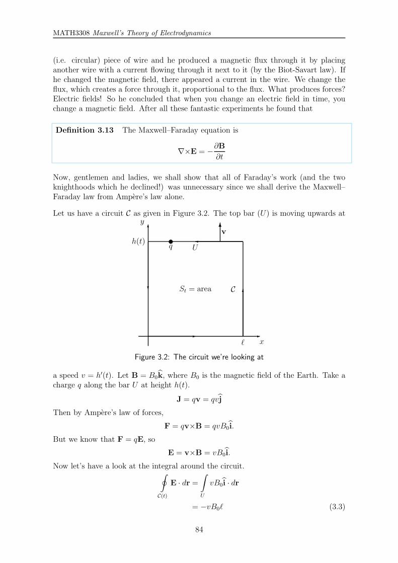
MATH3308 Maxwell’s Theory of Electrodynamics
(i.e. circular) piece of wire and he produced a magnetic flux through it by placinganother wire with a current flowing through it next to it (by the Biot-Savart law). Ifhe changed the magnetic field, there appeared a current in the wire. We change theflux, which creates a force through it, proportional to the flux. What produces forces?Electric fields! So he concluded that when you change an electric field in time, youchange a magnetic field. After all these fantastic experiments he found that
Definition 3.13 The Maxwell–Faraday equation is
∇×E = −∂B∂t
Now, gentlemen and ladies, we shall show that all of Faraday’s work (and the twoknighthoods which he declined!) was unnecessary since we shall derive the Maxwell–Faraday law from Ampere’s law alone.
Let us have a circuit C as given in Figure 3.2. The top bar (U) is moving upwards at
6y
-x
-ℓ
6C
U
6v
q
St = area?
h(t)
Figure 3.2: The circuit we’re looking at
a speed v = h′(t). Let B = B0k, where B0 is the magnetic field of the Earth. Take acharge q along the bar U at height h(t).
J = qv = qvj
Then by Ampere’s law of forces,
F = qv×B = qvB0i.
But we know that F = qE, so
E = v×B = vB0i.
Now let’s have a look at the integral around the circuit.∮
C(t)
E · dr =∫
U
vB0i · dr
= −vB0ℓ (3.3)
84

Chapter 3. Magnetism
and∫
St
B · n dS =
∫
St
B · k dS
=
∫
St
B0k · k dS
= B0
∫
St
dS
= B0 area(St)
= B0ℓh(t) (3.4)
=⇒ ∂
∂t
∫
St
B · n dS =d
dtB0ℓh(t)
= B0ℓv (3.5)
And by equating (3.3) and (3.5),
−∮
C(t)
E · dr = ∂
∂t
∫
St
B · n dS
or putting in the dependencies,
−∮
C(t)
E(x, t) · dr = ∂
∂t
∫
St
B(t) · n dS. (3.6)
Now here comes the trick. Say the change is not because of area, but instead becauseof changing flux. By Stokes’ law, the left hand side of equation (3.6) is equal to
−∮
C(t)
E(x, t) · dr =∫
S
(−∇×E) · n dS
and because S is not dependent on t, the right hand side of equation (3.6) is equal to
∂
∂t
∫
St
B(t) · n dS =
∫
St
∂B
∂t· n dS
i.e. ∫
S
(−∇×E) · n dS =
∫
St
∂B
∂t· n dS
And by the lemma we’re about to prove, since S is arbitrary, it’s safe to say that
∇×E = −∂B∂t.
85
MATH3308 Maxwell’s Theory of Electrodynamics
Lemma 3.14 The step above is valid.
Proof: Basically this step is valid because it’s a version of the DuBois-Reymondlemma. We start with ∫ (
∇×E+∂B
∂t
)· n dS = 0 (3.7)
and say that this is
⇐⇒ F := ∇×E+∂B
∂t= 0.
Why? Assume it is not zero at some point. Then there exists a point x0 such thatF(x0) 6= 0.
Take a plane Π perpendicular to F through the point x0, and call the disc of radius εin Π, Sε. We know that, by equation (3.7),
∫
Sε
F · n dS = 0.
But by our clever choice of plane,
n =F(x0)
|F(x0)|
And so
F · n|x=x0= |F(x0)| > 0.
But F is continuous on Π, so
F · n > 1
2|F(x0)|
if ε is sufficiently small. Thus
∫
Sε
F · n dS > 1
2|F(x0)| area(Sε)
> 0
which is a contradiction. Hence F(x) = 0 ∀x.
So we’ve proved the Maxwell–Faraday equation another way.
3.3 Maxwell’s equations
And so we have derived Maxwell’s equations in any material. Recalling that, formatrices ε and µ,
D = εE and B = µH,
In differential form:
86

Chapter 3. Magnetism
1. ∇ ·D = ρ Gauss’s law (Def .n 2.5)
2. ∇×E = −∂B∂t
Maxwell–Faraday equation (Def .n 3.13)
3. ∇ ·B = 0 Gauss’s law for magnetism (Def .n 3.7)
4. ∇×H =∂D
∂t+ J Maxwell–Ampere equation (Def .n 3.12)
In integral form:
1.
∫
S
D · n dS =
∫
V
ρ dV
2.
∫
C
E · dr = −∫
S
∂B
∂t· n dS
3.
∫
S
B · n dS = 0
4.
∫
C
H · dr =∫
S
(∂D
∂t+ J
)· n dS
3.4 Etude on differential forms
Coordinates do not come from God. What we want to be able to say is that Maxwell’sequations (particularly in integral form) are valid for any set of coordinates that wechoose to integrate along. So let’s have a brief discussion about differential forms.
∫
C
E · dr =∫
C
E1dx1 + E2dx
2 + E3dx3
Let x1 = x1(t), x2 = x2(t), x3 = x3(t), then
=
∫ b
a
[E1(x(t))
∂x1
∂tdt+ E2(x(t))
∂x2
∂tdt+ E3(x(t))
∂x3
∂tdt
]
=
∫ b
a
[E1(x(t))
∂x1
∂t+ E2(x(t))
∂x2
∂t+ E3(x(t))
∂x3
∂t
]dt
So what if xi = xi(yk), where i, k = 1, 2, 3, i.e. our x-coordinates are in terms ofy-coordinates, e.g. polars in Cartesians. Then
dx1 =∂x1
∂y1dy1 +
∂x1
∂y2dy2 +
∂x1
∂y3dy3
87

MATH3308 Maxwell’s Theory of Electrodynamics
and similarly for dx2 and dx3 so in this case,
∫
C
E · dr =∫
C
E1dx1 + E2dx
2 + E3dx3
=
∫ [E1∂x1
∂y1+ E2
∂x2
∂y1+ E3
∂x3
∂y1
]dy1
+
∫ [E1∂x1
∂y2+ E2
∂x2
∂y2+ E3
∂x3
∂y2
]dy2
+
∫ [E1∂x1
∂y3+ E2
∂x2
∂y3+ E3
∂x3
∂y3
]dy3
=
∫E · dy
where E is E in y-coordinates, i.e.
E1 =∂x
∂y1· E =
3∑
i=1
∂xi
∂y1Ei
or generally,
Ej =
3∑
i=1
∂xi
∂yjEi
so we can interchange3∑
i=1
Ei(x)dxi ←→
3∑
j=1
Ej(y)dyj
i.e. Maxwell’s equations are valid for any choice of coordinates. This means that wecan apply them, with suitable considerations of course, in any manifold.
3.4.1 Vectors and covectors
Velocity is a real vector.
vi =dxi
dt
=dxi(y)
dt
=
3∑
j=1
∂xi
∂yj∂yj
∂t
=3∑
j=1
∂xi
∂yjvj.
88

Chapter 3. Magnetism
See how we’re summing over j, in contrast to E, where we’re summing over i. So
v =
(∂x
∂y
)−1v
E =
(∂x
∂y
)T
E
So when you’re looking at a point, v is a vector, and E is a covector.
Generally, E,H are one-forms, and B,D are two-forms.
89

90

Chapter 4
Electromagnetic Waves
Solutions to Maxwell’s equations in the absence of sources and sinks, i.e. with ρ = 0,Jext = 0, are called electromagnetic waves.
Definition 4.1 Ohm’s law, as generalised by Gustav Kirchhoff, says that
J = Jext + σE
where σ is the conductivity matrix, a function of x and t. σ has to be positive definite.
In our study of (the very beginnings!) of the theory of electromagnetic waves we willalso assume that
σ = 0,
i.e. the conductivity is 0.
We will also assume that ε = ε(x), µ = µ(x), i.e. the electric and magnetic permitiv-ities are time-independent. These reduce Maxwell’s equations to
1. ∇ ·D = 0
2. ∇×E = −∂B∂t
3. ∇ ·B = 0
4. ∇×H =∂D
∂t
91

MATH3308 Maxwell’s Theory of Electrodynamics
4.1 Electromagnetic energy
Electromagnetic waves carry with them electromagnetic energy. The energy densityE(x, t) of this energy is given by
E(x, t) = 1
2[D · E+B ·H]
=1
2[(εE) · E+ (µH) ·H] . (4.1)
Now we look at how E changes with time t in some domain V ⊂ R3,
d
dt
∫
V
E(x, t) dV =
∫
V
∂E(x, t)∂t
dV
=
∫
V
∂
∂t
(1
2[(εE) · E+ (µH) ·H]
)dV
and using ∂∂t[(εE) · E] = 2
[∂∂t(εE) · E
],
=
∫
V
[(ε∂E
∂t
)·E+
(µ∂H
∂t
)·H]dV
=
∫
V
[∂D
∂t·E+
∂B
∂t·H]dV. (4.2)
Using what’s left of Maxwell’s equations, rewrite (4.2) as
=
∫
V
[(∇×H) · E−H · (∇×E)] dV
= −∫
V
∇ · (E×H) dV, (4.3)
where we use that −∇ · (a× b) = (∇×b) · a− b · (∇× a) for any vector fields a,b.
Problem 4.2 Show that
−∇ · (a× b) = (∇×b) · a− b · (∇× a)
Solution Let a =(
a1a2a3
)and b =
(b1b2b3
), and just do the computation. Boring but
trivial. X
Let’s now introduce the Poynting vector field.
92
Chapter 4. Electromagnetic Waves
Definition 4.3 The Poynting vector field S, named after its inventor John HenryPoynting, who was a professor at the University of Birmingham from 1880, is definedas
S = E×H.
With this definition, (4.3) gives rise to∫
V
∂E(x, t)∂t
dV = −∫
V
∇ · S dV
and then using the divergence theorem
= −∫
∂V
S · n dA, (4.4)
where dA is an area element and n is the exterior unit normal to ∂V .
Equation (4.4) implies that the Poynting vector S describes the flow of electromagneticenergy. Rewritten in the differential form it gives rise to the following continuityequation
∂E(x, t)∂t
+∇ · S(x, t) = 0,
cf. the charge continuity equation ∂ρ∂t
+∇ · J = 0.
Problem 4.4 Show that
∂E(x, t)∂t
+∇ · S(x, t) = 0.
Solution
∇ · S = ∇ · (E×H)
= (∇×E) ·H−E · (∇×H)
=
(−∂B∂t
)·H− E ·
(∂D
∂t
)
= −[(
∂B
∂t
)·H+ E ·
(∂D
∂t
)]
and
∂E∂t
=∂
∂t
1
2[D · E+B ·H]
=∂
∂t
1
2[(εE) ·E+ (µH) ·H]
=∂
∂t(εE) · E+
∂
∂t(µH) ·H
=∂D
∂t· E+
∂B
∂t·H
=⇒ ∂E∂t
+∇ · S = 0, as desired. X
93

MATH3308 Maxwell’s Theory of Electrodynamics
4.2 Electromagnetic waves in an homogeneous iso-
tropic medium
In the following we assume that the electric and magnetic permittivities ε and µ areisotropic and homogeneous (i.e. independent of x),
εij(x) = εδij µij(x) = µδij,
An example of such a medium is the vacuum, where ε = ε0, µ = µ0. An example ofone that is not is the brick that we introduced in section 3.2.1.
Rewriting Maxwell’s equations, taking into account the above,
1. ∇ ·D = 0
2. ∇×E = −µ∂H∂t
3. ∇ ·B = 0
4. ∇×H = ε∂E
∂t
Differentiating equations 2 and 4 with respect to t, we get
∇×(∂E
∂t
)= −µ∂
2H
∂t2
∇×(∂H
∂t
)= ε
∂2E
∂t2.
Using Maxwell’s equations as rewritten above, for ∂E∂t, ∂H
∂t, we get
∇× (∇×H) = −εµ∂2H
∂t2(4.5)
∇× (∇×E) = −εµ∂2E
∂t2. (4.6)
Recall that, by the definition of the vector Laplacian ∇2H,
∇× (∇×H) = ∇ (∇ ·H)−∇2H,
where∇2H = (∇2H1,∇2H2,∇2H3).
Then using equation 3 in Maxwell’s equations, ∇ ·H = 0, so we get
∇× (∇×H) = −∇2H
and (4.5) becomes∂2H
∂t2=
1
εµ∇2H.
Similarly we can also derive∂2E
∂t2=
1
εµ∇2E.
94

Chapter 4. Electromagnetic Waves
Problem 4.5 Derive∂2E
∂t2=
1
εµ∇2E.
Component wise, this is equivalent to six scalar wave equations for the componentsEi(x, t), Hi(x, t), where i = 1, 2, 3,
∂2Ei(x, t)
∂t2− c2∇2Ei(x, t) = 0
∂2Hi(x, t)
∂t2− c2∇2Hi(x, t) = 0, (4.7)
where
c =1√εµ
(4.8)
is the speed of electromagnetic waves (the speed of light) in the medium. (Note thatin vacuum, c0 =
1√ε0µ0
).
4.3 Plane waves
An important special case of electromagnetic waves are the plane waves. In this case,E and H depend, in addition to t, only on one space variable xe = x · e, wheree = (e1, e2, e3) is a unit vector. Since we’re in isotropic material, we can take e = i,and xe = x1. Explicitly,
E = E(x1, t) H = H(x1, t) (4.9)
Clearly, in this case, E and H remain the same, at any fixed time t, in any planeorthogonal to i, which explains the name “plane waves”. Then, the 3D wave equations(4.7) become 1D wave equations (which we studied in MATH1302∗),
∂2Ei(x1, t)
∂t2− c2∂
2Ei(x1, t)
∂x21= 0
∂2Hi(x1, t)
∂t2− c2∂
2Hi(x1, t)
∂x21= 0 (4.10)
We also do know the general solution in this case,
Ei(x, t) = E+i (x1 + ct) + E−i (x1 − ct)
Hi(x, t) = H+i (x1 + ct) +H−i (x1 − ct). (4.11)
i.e. in each case we have the superposition of two waves, one going to the right andone going to the left.
∗LOL
95
MATH3308 Maxwell’s Theory of Electrodynamics
Problem 4.6 Show that if E = E(x1, t), H = H(x1, t), then
Ei(x, t) = E+i (x1 + ct) + E−i (x1 − ct)
Hi(x, t) = H+i (x1 + ct) +H−i (x1 − ct)
for i = 1, 2, 3 and some functions E±i (x1), H±i (x1).
Solution Look at the wave equation
∂2f
∂t2= c2∇2f,
assuming that f = f(x1, t).
Use the substitutionζ = x1 − ct η = x1 + ct
Then
∂f
∂η=
∂f
∂x1
∂x1∂η
+∂f
∂t
∂t
∂η
=∂f
∂x1+
1
c
∂f
∂t
:= F (x1, t)
∂2f
∂ζ∂η=
∂
∂ζ
(∂f
∂x1+
1
c
∂f
∂t
)
=∂F
∂x1
∂x1∂ζ
+∂F
∂t
∂t
∂ζ
=
(∂2f
∂x21+
1
c
∂2f
∂x1∂t
)+
(∂2f
∂x1∂t+
1
c
∂2f
∂t2
)·(−1c
)
=∂2f
∂x21− 1
c2∂2f
∂t2
=∂2f
∂x21− 1
c2(c2∇2f)
=∂2f
∂x21− ∂2f
∂x21= 0.
So∂F
∂ζ= 0
since F = ∂f∂η. Therefore F is an arbitrary function of η: F = F (η). That is to say
∂f
∂η= F (η),
an arbitrary function of η. Sof = α(η) + β(ζ)
96

Chapter 4. Electromagnetic Waves
where
α(η) =
∫ η
0
F (η) dη
hence
f = α(x1 − ct) + β(x1 + ct)
X
This formula shows that, indeed, the waves propagate with speed c in the i-direction,or, more precisely, E(x1 − ct),H(x1 − ct) is the wave propagating in the i-direction
while E(x1 + ct),H(x1 + ct) is the wave propagating in the −i-direction. Note thatto satisfy Maxwell’s equations, each of these two waves should satisfy these equationsinpedendently.
Using the original Maxwell equations, rather than the 1D wave equation (4.7), we canfurther analyse E,H in this case. However, we will concentrate on one special type ofplane waves.
4.4 Harmonic plane waves
An electromagnetic wave is harmonic if its dependence on t is periodic and of the forme±iωt, where ω is the frequency of oscillation. Thus, a harmonic electromagnetic wavehas the form
E(x, t) = E+(x)eiωt + E−(x)e−iωt,
H(x, t) = H+(x)eiωt +H−(x)e−iωt.
If the electromagnetic wave is harmonic and plane, then the above equation, togetherwith (4.11), implies that
E(x, t) = E+ei(kx1+ωt) + E−ei(kx1−ωt) + complex conjugate
H(x, t) = H+ei(kx1+ωt) +H−ei(kx1−ωt) + complex conjugate, (4.12)
where E±,H± are (complex) constant vectors and ωk= c.
Again, to satisfy Maxwell’s equations, each of the terms in these two sums of fourterms should satisfy them. Thus, it is sufficient to concentrate on, say, E−ei(kx1−ωt)
and H−ei(kx1−ωt). We’ll drop the minus sign to signal our generalisation.
Recall the divergence pair of Maxwell’s equations: ∇·B = ∇·D = 0. Obviously then∇ ·H = ∇ · E = 0 so
0 = ∇ ·(Eei(kx1−ωt))
= (E · i)ikei(kx1−ωt)
=⇒ 0 = (E · i)
97

MATH3308 Maxwell’s Theory of Electrodynamics
and similarly
=⇒ 0 = (H · i) (4.13)
i.e. E,H lie in the plane orthogonal to the direction of the wave propagation i.
Next, the Maxwell-Faraday equation tells that
∇×E = −∂B∂t
= −µ∂H∂t
and (4.12) tells us that
−µ∂H∂t
= ickµH
And we can work out that∇×E = ik(i×E)
Problem 4.7 Show that∇×E = ik(i×E)
Solution Recall that from equation (4.9), E = E(x1, t). So
∇×E =
∣∣∣∣∣∣
i j k∂
∂x1
∂∂x2
∂∂x3
E1(x1, t) E2(x1, t) E3(x1, t)
∣∣∣∣∣∣
=∂E2
∂x1k− ∂E3
∂x1j
which by equation (4.12),
= ik(E2k−E3j)
and on the other side,
ik(i×E) = ik
∣∣∣∣∣∣
i j k1 0 0
E1(x1, t) E2(x1, t) E3(x1, t)
∣∣∣∣∣∣
= ik(E2k−E3j)
which is clearly equivalent. X
so this implies
H =1
cµ(i× E) (4.14)
=
√ε
µ(i× E)
=1
Z(i×E)
98

Chapter 4. Electromagnetic Waves
where
Z =
õ
ε
is called the electromagnetic impedance.
Similarly, the Maxwell-Ampere equation implies that
E = −Z i×H. (4.15)
Note that (4.15) follows from (4.14) if we apply i× to both parts.
Let us analyse these equations. In principle, E is a complex vector. By shifting t, wecan assume
E = E1u1 + E2eiαu2,
where E1, E2 are positive and u1,u2, i form a right-hand triple of orthonormal vectors.Then,
ZH = E1u2 − E2eiαu1.
This means that the real parts of E and H are orthogonal, and the same is true fortheir imaginary parts.
The last remark is about polarisation. When α ∈ 0,±π, then the direction ofE exp i(kx1 − ωt) does not depend on (x, t): we have linearly polarised waves sinceeiα = ±1. However, for other α, if we fix any x, the direction of physical electric field(which is the real part of E exp i(kx1 − ωt)) will rotate with period T = 2π
ω.
For example, if E1 = E2 and α = π2
Ephysical(x, t) = E1 (cos(kx1 − ωt)u1 − sin(kx1 − ωt)u2) .
which gives you an ellipse.
Problem 4.8 Let α 6= π2,u2 6= 0. So eiα is not real. Find the formula of Ephysical
and show that we get a slanted ellipse.
This problem is left as an exercise for the reader!
And that concludes our study of Maxwell’s Theory of Electrodynamics. The exam in2011, for which these notes were given, featured two questions from chapter 1, twoquestions from chapters 2 and 3, and one question from chapter 4. Please report anyerrors you have noticed in the document to the editors, whose details can be found onpage 4. Chocolate, beer and any other form of appreciation will be warmly received.
谢谢
99

MATH3308 Maxwell’s Theory of Electrodynamics
Figure 4.1: Class of 2011
100