Matrix Algebra in R

William RevelleNorthwestern University

January 24, 2007

Prepared as part of a course on Latent Variable Modeling, Winter, 2007

and as a supplement to the Guide to R for psychologists.

email comments to: revelle@northwestern.edu

A Matrix Algebra in R 2A.1 Vectors . . . . . . . . . . . . . . . . . . . . . . . . . . . . . . . . . . . . . . . . 2

A.1.1 Vector multiplication . . . . . . . . . . . . . . . . . . . . . . . . . . . . . 3A.1.2 Simple statistics using vectors . . . . . . . . . . . . . . . . . . . . . . . . 5A.1.3 Combining vectors . . . . . . . . . . . . . . . . . . . . . . . . . . . . . . 7

A.2 Matrices . . . . . . . . . . . . . . . . . . . . . . . . . . . . . . . . . . . . . . . . 8A.2.1 Matrix addition . . . . . . . . . . . . . . . . . . . . . . . . . . . . . . . . 9A.2.2 Matrix multiplication . . . . . . . . . . . . . . . . . . . . . . . . . . . . 10A.2.3 Finding and using the diagonal . . . . . . . . . . . . . . . . . . . . . . . 12A.2.4 The Identity Matrix . . . . . . . . . . . . . . . . . . . . . . . . . . . . . 13A.2.5 Matrix Inversion . . . . . . . . . . . . . . . . . . . . . . . . . . . . . . . 13

A.3 Matrix operations for data manipulation . . . . . . . . . . . . . . . . . . . . . . 14A.3.1 Matrix operations on the raw data . . . . . . . . . . . . . . . . . . . . . 16A.3.2 Matrix operations on the correlation matrix . . . . . . . . . . . . . . . . 16A.3.3 Using matrices to find test reliability . . . . . . . . . . . . . . . . . . . . 17

A.4 Multiple correlation . . . . . . . . . . . . . . . . . . . . . . . . . . . . . . . . . 18A.4.1 Data level analyses . . . . . . . . . . . . . . . . . . . . . . . . . . . . . . 19A.4.2 Non optimal weights and the goodness of fit . . . . . . . . . . . . . . . . 21

1

Appendix A

Matrix Algebra in R

Much of psychometrics in particular, and psychological data analysis in general consists ofoperations on vectors and matrices. This appendix offers a quick review of matrix oper-ations with a particular emphasis upon how to do matrix operations in R. For more in-formation on how to use R, consult the short guide to R for psychologists (at http://personality-project.org/r/r.guide.html) or the even shorter guide at personality-project.org/r/r.205.tutorial.html.

A.1 Vectors

A vector is a one dimensional array of n numbers. Basic operations on a vector are additionand subtraction. Multiplication is somewhat more complicated, for the order in which twovectors are multiplied changes the result. That is AB 6= BA.

Consider V1 = the first 10 integers, and V2 = the next 10 integers:

> V1 <- as.vector(seq(1, 10))

[1] 1 2 3 4 5 6 7 8 9 10

> V2 <- as.vector(seq(11, 20))

[1] 11 12 13 14 15 16 17 18 19 20

We can add a constant to each element in a vector

> V4 <- V1 + 20

[1] 21 22 23 24 25 26 27 28 29 30

or we can add each element of the first vector to the corresponding element of the secondvector

> V3 <- V1 + V2

[1] 12 14 16 18 20 22 24 26 28 30

2

Strangely enough, a vector in R is dimensionless, but it has a length. If we want to multiplytwo vectors, we first need to think of the vector either as row or as a column. A columnvector can be made into a row vector (and vice versa) by the transpose operation. While avector has no dimensions, the transpose of a vector is two dimensional! It is a matrix withwith 1 row and n columns. (Although the dim command will return no dimensions, in termsof multiplication, a vector is a matrix of n rows and 1 column.)

Consider the following:

> dim(V1)

NULL

> length(V1)

[1] 10

> dim(t(V1))

[1] 1 10

> dim(t(t(V1)))

[1] 10 1

> TV <- t(V1)

[,1] [,2] [,3] [,4] [,5] [,6] [,7] [,8] [,9] [,10][1,] 1 2 3 4 5 6 7 8 9 10

> t(TV)

[,1][1,] 1[2,] 2[3,] 3[4,] 4[5,] 5[6,] 6[7,] 7[8,] 8[9,] 9[10,] 10

A.1.1 Vector multiplication

Just as we can add a number to every element in a vector, so can we multiply a number(a“scaler”) by every element in a vector.

> V2 <- 4 * V1

[1] 4 8 12 16 20 24 28 32 36 40

3

There are three types of multiplication of vectors in R. Simple multiplication (each term inone vector is multiplied by its corresponding term in the other vector), as well as the innerand outer products of two vectors.

Simple multiplication requires that each vector be of the same length. Using the V1 and V2vectors from before, we can find the 10 products of their elements:

> V1

[1] 1 2 3 4 5 6 7 8 9 10

> V2

[1] 4 8 12 16 20 24 28 32 36 40

> V1 * V2

[1] 4 16 36 64 100 144 196 256 324 400

The “outer product” of a n * 1 element vector with a 1 * m element vector will result in a n* m element matrix. (The dimension of the resulting product is the outer dimensions of thetwo vectors in the multiplication). The vector multiply operator is %*%. In the followingequation, the subscripts refer to the dimensions of the variable.

nX1 ∗1 Ym =n (XY )m (A.1)

> V1 <- seq(1, 10)

> V2 <- seq(1, 4)

> V1

[1] 1 2 3 4 5 6 7 8 9 10

> V2

[1] 1 2 3 4

> outer.prod <- V1 %*% t(V2)

> outer.prod

[,1] [,2] [,3] [,4][1,] 1 2 3 4[2,] 2 4 6 8[3,] 3 6 9 12[4,] 4 8 12 16[5,] 5 10 15 20[6,] 6 12 18 24[7,] 7 14 21 28[8,] 8 16 24 32[9,] 9 18 27 36[10,] 10 20 30 40

The outer product of the first ten integers is, of course, the multiplication table known to allelementary school students:

4

> outer.prod <- V1 %*% t(V1)

[,1] [,2] [,3] [,4] [,5] [,6] [,7] [,8] [,9] [,10][1,] 1 2 3 4 5 6 7 8 9 10[2,] 2 4 6 8 10 12 14 16 18 20[3,] 3 6 9 12 15 18 21 24 27 30[4,] 4 8 12 16 20 24 28 32 36 40[5,] 5 10 15 20 25 30 35 40 45 50[6,] 6 12 18 24 30 36 42 48 54 60[7,] 7 14 21 28 35 42 49 56 63 70[8,] 8 16 24 32 40 48 56 64 72 80[9,] 9 18 27 36 45 54 63 72 81 90[10,] 10 20 30 40 50 60 70 80 90 100

The “inner product” is perhaps a more useful operation, for it not only multiplies each corre-sponding element of two vectors, but also sums the resulting product:

inner.product =N∑

i=1

V 1i ∗ V 2i (A.2)

> V1 <- seq(1, 10)

> V2 <- seq(11, 20)

> V1

[1] 1 2 3 4 5 6 7 8 9 10

> V2

[1] 11 12 13 14 15 16 17 18 19 20

> in.prod <- t(V1) %*% V2

> in.prod

[,1][1,] 935

Note that the inner product of two vectors is of length =1 but is a matrix with 1 row and 1column. (This is the dimension of the inner dimensions (1) of the two vectors.)

A.1.2 Simple statistics using vectors

Although there are built in functions in R to do most of our statistics, it is useful to understandhow these operations can be done using vector and matrix operations. Here we consider howto find the mean of a vector, remove it from all the numbers, and then find the averagesquared deviation from the mean (the variance).

Consider the mean of all numbers in a vector. To find this we just need to add up the numbers(the inner product of the vector with a vector of 1’s) and then divide by n (multiply by thescaler 1/n). First we create a vector of 1s by using the repeat operation. We then show threedifferent equations for the mean.V, all of which are equivalent.

5

> V <- V1

[1] 1 2 3 4 5 6 7 8 9 10

> one <- rep(1, length(V))

[1] 1 1 1 1 1 1 1 1 1 1

> sum.V <- t(one) %*% V

[,1][1,] 55

> mean.V <- sum.V * (1/length(V))

[,1][1,] 5.5

> mean.V <- t(one) %*% V * (1/length(V))

[,1][1,] 5.5

> mean.V <- t(one) %*% V/length(V)

[,1][1,] 5.5

The variance is the average squared deviation from the mean. To find the variance, we firstfind deviation scores by subtracting the mean from each value of the vector. Then, to findthe sum of the squared deviations take the inner product of the result with itself. This Sumof Squares becomes a variance if we divide by the degrees of freedom (n-1) to get an unbiasedestimate of the population variance). First we find the mean centered vector:

> V - mean.V

[1] -4.5 -3.5 -2.5 -1.5 -0.5 0.5 1.5 2.5 3.5 4.5

And then we find the variance as the mean square by taking the inner product:

> Var.V <- t(V - mean.V) %*% (V - mean.V) * (1/(length(V) - 1))

[,1][1,] 9.166667

Compare these results with the more typical scale, mean and var operations:

> scale(V, scale = FALSE)

[,1][1,] -4.5[2,] -3.5[3,] -2.5[4,] -1.5[5,] -0.5[6,] 0.5[7,] 1.5

6

[8,] 2.5[9,] 3.5[10,] 4.5attr(,"scaled:center")[1] 5.5

> mean(V)

[1] 5.5

> var(V)

[1] 9.166667

A.1.3 Combining vectors

We can form more complex data structures than vectors by combining the vectors, either bycolumns (cbind) or by rows (rbind). The resulting data structure is a matrix.

> Xc <- cbind(V1, V2, V3)

V1 V2 V3[1,] 1 11 12[2,] 2 12 14[3,] 3 13 16[4,] 4 14 18[5,] 5 15 20[6,] 6 16 22[7,] 7 17 24[8,] 8 18 26[9,] 9 19 28[10,] 10 20 30

> Xr <- rbind(V1, V2, V3)

[,1] [,2] [,3] [,4] [,5] [,6] [,7] [,8] [,9] [,10]V1 1 2 3 4 5 6 7 8 9 10V2 11 12 13 14 15 16 17 18 19 20V3 12 14 16 18 20 22 24 26 28 30

> dim(Xc)

[1] 10 3

> dim(Xr)

[1] 3 10

7

A.2 Matrices

A matrix is just a two dimensional (rectangular) organization of numbers. It is a vector ofvectors. For data analysis, the typical data matrix is organized with columns representingdifferent variables and rows containing the responses of a particular subject. Thus, a 10 x4 data matrix (10 rows, 4 columns) would contain the data of 10 subjects on 4 differentvariables. Note that the matrix operation has taken the numbers 1 through 40 and organizedthem column wise. That is, a matrix is just a way (and a very convenient one at that) oforganizing a vector.

R provides numeric row and column names (e.g., [1,] is the first row, [,4] is the fourth column,but it is useful to label the rows and columns to make the rows (subjects) and columns(variables) distinction more obvious. 1

> Xij <- matrix(seq(1:40), ncol = 4)

> rownames(Xij) <- paste("S", seq(1, dim(Xij)[1]), sep = "")

> colnames(Xij) <- paste("V", seq(1, dim(Xij)[2]), sep = "")

> Xij

V1 V2 V3 V4S1 1 11 21 31S2 2 12 22 32S3 3 13 23 33S4 4 14 24 34S5 5 15 25 35S6 6 16 26 36S7 7 17 27 37S8 8 18 28 38S9 9 19 29 39S10 10 20 30 40

Just as the transpose of a vector makes a column vector into a row vector, so does thetranspose of a matrix swap the rows for the columns. Note that now the subjects are columnsand the variables are the rows.

> t(Xij)

S1 S2 S3 S4 S5 S6 S7 S8 S9 S10V1 1 2 3 4 5 6 7 8 9 10V2 11 12 13 14 15 16 17 18 19 20V3 21 22 23 24 25 26 27 28 29 30V4 31 32 33 34 35 36 37 38 39 40

1Although many think of matrices as developed in the 17th century, O’Conner and Robertson discuss thehistory of matrix algebra back to the Babylonians (http://www-history.mcs.st-andrews.ac.uk/history/HistTopics/Matrices_and_determinants.html)

8

A.2.1 Matrix addition

The previous matrix is rather uninteresting, in that all the columns are simple products ofthe first column. A more typical matrix might be formed by sampling from the digits 0-9.For the purpose of this demonstration, we will set the random number seed to a memorablenumber so that it will yield the same answer each time.

> set.seed(42)

> Xij <- matrix(sample(seq(0, 9), 40, replace = TRUE), ncol = 4)

> rownames(Xij) <- paste("S", seq(1, dim(Xij)[1]), sep = "")

> colnames(Xij) <- paste("V", seq(1, dim(Xij)[2]), sep = "")

> print(Xij)

V1 V2 V3 V4S1 9 4 9 7S2 9 7 1 8S3 2 9 9 3S4 8 2 9 6S5 6 4 0 0S6 5 9 5 8S7 7 9 3 0S8 1 1 9 2S9 6 4 4 9S10 7 5 8 6

Just as we could with vectors, we can add, subtract, muliply or divide the matrix by a scaler(a number with out a dimension).

> Xij + 4

V1 V2 V3 V4S1 13 8 13 11S2 13 11 5 12S3 6 13 13 7S4 12 6 13 10S5 10 8 4 4S6 9 13 9 12S7 11 13 7 4S8 5 5 13 6S9 10 8 8 13S10 11 9 12 10

> round((Xij + 4)/3, 2)

V1 V2 V3 V4S1 4.33 2.67 4.33 3.67S2 4.33 3.67 1.67 4.00S3 2.00 4.33 4.33 2.33S4 4.00 2.00 4.33 3.33S5 3.33 2.67 1.33 1.33

9

S6 3.00 4.33 3.00 4.00S7 3.67 4.33 2.33 1.33S8 1.67 1.67 4.33 2.00S9 3.33 2.67 2.67 4.33S10 3.67 3.00 4.00 3.33

We can also multiply each row (or column, depending upon order) by a vector.

> V

[1] 1 2 3 4 5 6 7 8 9 10

> Xij * V

V1 V2 V3 V4S1 9 4 9 7S2 18 14 2 16S3 6 27 27 9S4 32 8 36 24S5 30 20 0 0S6 30 54 30 48S7 49 63 21 0S8 8 8 72 16S9 54 36 36 81S10 70 50 80 60

A.2.2 Matrix multiplication

Matrix multiplication is a combination of multiplication and addition. For a matrix mXn ofdimensions m*n and nYp of dimension n * p, the product, mXYp is a m * p matrix where eachelement is the sum of the products of the rows of the first and the columns of the second.That is, the matrix mXYp has elements xyij where each

xyij =n∑

k=1

xik ∗ yjk (A.3)

Consider our matrix Xij with 10 rows of 4 columns. Call an individual element in this matrixxij . We can find the sums for each column of the matrix by multiplying the matrix by our“one” vector with Xij. That is, we can find

∑Ni=1 Xij for the j columns, and then divide by the

number (n) of rows. (Note that we can get the same result by finding colMeans(Xij).

We can use the dim function to find out how many cases (the number of rows) or the numberof variables (number of columns). dim has two elements: dim(Xij)[1] = number of rows,dim(Xij)[2] is the number of columns.

> dim(Xij)

[1] 10 4

> n <- dim(Xij)[1]

10

[1] 10

> one <- rep(1, n)

[1] 1 1 1 1 1 1 1 1 1 1

> X.means <- t(one) %*% Xij/n

V1 V2 V3 V4[1,] 6 5.4 5.7 4.9

A built in function to find the means of the columns is colMeans. (See rowMeans for theequivalent for rows.)

> colMeans(Xij)

V1 V2 V3 V46.0 5.4 5.7 4.9

Variances and covariances are measures of dispersion around the mean. We find these by firstsubtracting the means from all the observations. This means centered matrix is the originalmatrix minus a matrix of means. To make them have the same dimensions we premultiplythe means vector by a vector of ones and subtract this from the data matrix.

> X.diff <- Xij - one %*% X.means

V1 V2 V3 V4S1 3 -1.4 3.3 2.1S2 3 1.6 -4.7 3.1S3 -4 3.6 3.3 -1.9S4 2 -3.4 3.3 1.1S5 0 -1.4 -5.7 -4.9S6 -1 3.6 -0.7 3.1S7 1 3.6 -2.7 -4.9S8 -5 -4.4 3.3 -2.9S9 0 -1.4 -1.7 4.1S10 1 -0.4 2.3 1.1

To find the variance/covariance matrix, we can first find the the inner product of the meanscentered matrix X.diff = Xij - X.means t(Xij-X.means) with itself and divide by n-1. Wecan compare this result to the result of the cov function (the normal way to find covari-ances).

> X.cov <- t(X.diff) %*% X.diff/(n - 1)

> round(X.cov, 2)

V1 V2 V3 V4V1 7.33 0.11 -3.00 3.67V2 0.11 8.71 -3.20 -0.18V3 -3.00 -3.20 12.68 1.63V4 3.67 -0.18 1.63 11.43

> round(cov(Xij), 2)

11

V1 V2 V3 V4V1 7.33 0.11 -3.00 3.67V2 0.11 8.71 -3.20 -0.18V3 -3.00 -3.20 12.68 1.63V4 3.67 -0.18 1.63 11.43

A.2.3 Finding and using the diagonal

Some operations need to find just the diagonal. For instance, the diagonal of the matrix X.cov(found above) contains the variances of the items. To extract just the diagonal, or create amatrix with a particular diagonal we use the diag command. We can convert the covariancematrix X.cov to a correlation matrix X.cor by pre and post multiplying the covariance matrixwith a diagonal matrix containing the reciprocal of the standard deviations (square rootsof the variances). Remember that the correlation, rxy, is merely the covariancexy/

√VxVy.

Compare this to the standard command for finding correlations cor.

> round(X.cov, 2)

V1 V2 V3 V4V1 7.33 0.11 -3.00 3.67V2 0.11 8.71 -3.20 -0.18V3 -3.00 -3.20 12.68 1.63V4 3.67 -0.18 1.63 11.43

> round(diag(X.cov), 2)

V1 V2 V3 V47.33 8.71 12.68 11.43

> sdi <- diag(1/sqrt(diag(X.cov)))

> rownames(sdi) <- colnames(sdi) <- colnames(X.cov)

> round(sdi, 2)

V1 V2 V3 V4V1 0.37 0.00 0.00 0.0V2 0.00 0.34 0.00 0.0V3 0.00 0.00 0.28 0.0V4 0.00 0.00 0.00 0.3

> X.cor <- sdi %*% X.cov %*% sdi

> rownames(X.cor) <- colnames(X.cor) <- colnames(X.cov)

> round(X.cor, 2)

V1 V2 V3 V4V1 1.00 0.01 -0.31 0.40V2 0.01 1.00 -0.30 -0.02V3 -0.31 -0.30 1.00 0.14V4 0.40 -0.02 0.14 1.00

> round(cor(Xij), 2)

12

V1 V2 V3 V4V1 1.00 0.01 -0.31 0.40V2 0.01 1.00 -0.30 -0.02V3 -0.31 -0.30 1.00 0.14V4 0.40 -0.02 0.14 1.00

A.2.4 The Identity Matrix

The identity matrix is merely that matrix, which when multiplied by another matrix, yieldsthe other matrix. (The equivalent of 1 in normal arithmetic.) It is a diagonal matrix with 1on the diagonal I <- diag(1,nrow=dim(X.cov)[1],ncol=dim(X.cov)[2])

A.2.5 Matrix Inversion

The inverse of a square matrix is the matrix equivalent of dividing by that matrix. Thatis, either pre or post multiplying a matrix by its inverse yields the identity matrix. Theinverse is particularly important in multiple regression, for it allows is to solve for the betaweights.

Given the equationY = bX + c (A.4)

we can solve for b by multiplying both sides of the equation by

X−1orY X−1 = bXX−1 = b (A.5)

We can find the inverse by using the solve function. To show that XX−1 = X−1X = I, wedo the multiplication.

> X.inv <- solve(X.cov)

V1 V2 V3 V4V1 0.19638636 0.01817060 0.06024476 -0.07130491V2 0.01817060 0.12828756 0.03787166 -0.00924279V3 0.06024476 0.03787166 0.10707738 -0.03402838V4 -0.07130491 -0.00924279 -0.03402838 0.11504850

> round(X.cov %*% X.inv, 2)

V1 V2 V3 V4V1 1 0 0 0V2 0 1 0 0V3 0 0 1 0V4 0 0 0 1

> round(X.inv %*% X.cov, 2)

V1 V2 V3 V4V1 1 0 0 0

13

V2 0 1 0 0V3 0 0 1 0V4 0 0 0 1

There are multiple ways of finding the matrix inverse, solve is just one of them.

A.3 Matrix operations for data manipulation

Using the basic matrix operations of addition and multiplication allow for easy manipulationof data. In particular, finding subsets of data, scoring multiple scales for one set of items, orfinding correlations and reliabilities of composite scales are all operations that are easy to dowith matrix operations.

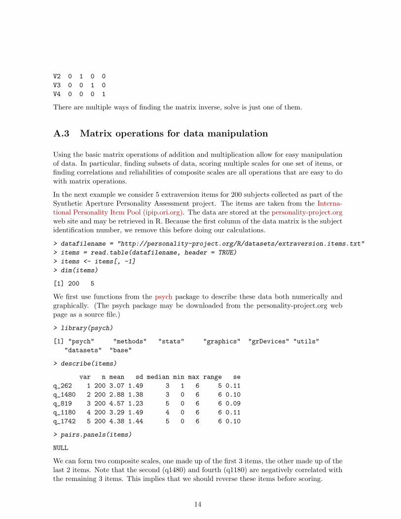
In the next example we consider 5 extraversion items for 200 subjects collected as part of theSynthetic Aperture Personality Assessment project. The items are taken from the Interna-tional Personality Item Pool (ipip.ori.org). The data are stored at the personality-project.orgweb site and may be retrieved in R. Because the first column of the data matrix is the subjectidentification number, we remove this before doing our calculations.

> datafilename = "http://personality-project.org/R/datasets/extraversion.items.txt"

> items = read.table(datafilename, header = TRUE)

> items <- items[, -1]

> dim(items)

[1] 200 5

We first use functions from the psych package to describe these data both numerically andgraphically. (The psych package may be downloaded from the personality-project.org webpage as a source file.)

> library(psych)

[1] "psych" "methods" "stats" "graphics" "grDevices" "utils""datasets" "base"

> describe(items)

var n mean sd median min max range seq_262 1 200 3.07 1.49 3 1 6 5 0.11q_1480 2 200 2.88 1.38 3 0 6 6 0.10q_819 3 200 4.57 1.23 5 0 6 6 0.09q_1180 4 200 3.29 1.49 4 0 6 6 0.11q_1742 5 200 4.38 1.44 5 0 6 6 0.10

> pairs.panels(items)

NULL

We can form two composite scales, one made up of the first 3 items, the other made up of thelast 2 items. Note that the second (q1480) and fourth (q1180) are negatively correlated withthe remaining 3 items. This implies that we should reverse these items before scoring.

14

q_262

0 2 4 6

−0.26 0.41

0 2 4 6

−0.51

12

34

56

0.48

02

46

● ●●

●

●

●

●

●●

●

●

●

●

●

●

●●

●

●

●

●

●

●

●

●

●

●

●

●

●

●●

●

●

●●

●

●

●

●

●

●

●

●

●●

●

●

●

●

●● ●

●

●

●

●

●

●

●

●

●

●●

●●

●

●

●

●● ●

●

●

●

●

●

●

●

●

●

●

● ●

●

●●

●

●

●

●

●

●

●

●

●

●

● ●

●

●

●

●● ●

●●

●

● ●●

●

●

●●

● ●

●●

●

●

●

●

●

●●●

●

●

●

●

●●

●

●●

●

●

●

●

●

●

●

●

●●

●

●

●

●

●

●

●

●

●

●●●

● ●● ●

●

●

●

●

●

● ●

●●●

●

●

●

●

●

●●

●

●●

●

●

●

●●

●

●

●

●

●

●

●

●●

● ●●●

q_1480−0.66 0.52 −0.47

● ●●

●

●

●●

●●

●

●●

● ●

●

●● ●

●

●●

●

●

●

●

●

●

●

●

●

●

●

●

●

●●●

●

●

●

●

●

●

●

●

● ●●●

●

●

● ●

●

●

●

●

● ●

●

●

●

●

●

●

●

●

●

● ●

●

●●●

●

●●

●

●

●

●

●●

●

●

●

●

●

●

●

●

●

● ●

●

●●

● ●

●

●

●

●

●

● ●

●

●●

●●

●

●

●●

● ●

●●

●●

●

●

●●●● ●

●

● ●●●

●

●●

●

●

●

●

●

●

●

●

●

●

●

●

●

●●

●●

●

●

●

●

●

●

●

● ●

●

●

●

●

●

●

●●

●●

●●

●

●

●

●●

●

●●

●

●

● ●

●

●

●

●

●

●

●●●● ● ●

●●

●●●

●

●

● ●

●●

●

●●

● ●

●

●● ●

●

● ●

●

●

●

●

●

●

●

●

●

●

●

●

●

●●●

●

●

●

●

●

●

●

●

●●● ●

●

●

●●

●

●

●

●

● ●

●

●

●

●

●

●

●

●

●

●●

●

●● ●

●

●●

●

●

●

●

●●

●

●

●

●

●

●

●

●

●

● ●

●

● ●

●●

●

●

●

●

●

●●

●

● ●

●●

●

●

●●

●●

●●

●●

●

●

●●●● ●

●

● ●●●

●

●●

●

●

●

●

●

●

●

●

●

●

●

●

●

●●

●●

●

●

●

●

●

●

●

●●

●

●

●

●

●

●

●●

●●

●●

●

●

●

●●

●

●●

●

●

● ●

●

●

●

●

●

●

● ●●● ●●

●●

q_819−0.41

02

46

0.65

02

46

●

●●

●

●

●

●

●●

●

●●●

●

●

●● ●●●

●

●

●

●

●●

●

●

●

● ●●

●

●

●●

●

●

●●

●

●

●

●●

●

●

●●

●

●

●

●● ●●

●

●

●

●

●

●

●●

●●

●●

● ●●

●

●

●

●

●

●

●

●●

●

●

● ●●

●

●

●● ●●

●●

●

●

●

●

●

●

●

●● ●

●

●

●

●

●

●

●

●● ●

●

●

●

●

●

●

●

●

●

●●

●●●

●

●

●

●

●

●

●●

●

●

●

●

●

●

●

●

●●

●

●

●

●

●● ●●●

●

●●

●

●

●

●

●

●

●●

●

●

●

●

●

●●

●●

●

●

●

●

●

●

●

●

●

●

●

●

●

●

●

●

●

●

●

●

●●

●

●

●● ●

●●

●

●

●

●

●●

●

●●●

●

●

●● ●●●

●

●

●

●

●●

●

●

●

●●●

●

●

●●

●

●

●●

●

●

●

● ●

●

●

● ●

●

●

●

●● ●●

●

●

●

●

●

●

●●

●●

●●

●●●

●

●

●

●

●

●

●

● ●

●

●

●●●

●

●

● ●● ●

● ●

●

●

●

●

●

●

●

● ● ●

●

●

●

●

●

●

●

●● ●

●

●

●

●

●

●

●

●

●

● ●

●●●

●

●

●

●

●

●

●●

●

●

●

●

●

●

●

●

●●

●

●

●

●

●● ●● ●

●

●●

●

●

●

●

●

●

●●

●

●

●

●

●

●●

●●

●

●

●

●

●

●

●

●

●

●

●

●

●

●

●

●

●

●

●

●

●●

●

●

●● ●

●●

●

●

●

●

●●

●

●● ●

●

●

●●●● ●

●

●

●

●

● ●

●

●

●

● ●●

●

●

●●

●

●

● ●

●

●

●

●●

●

●

●●

●

●

●

● ●● ●

●

●

●

●

●

●

●●

● ●

● ●

●● ●

●

●

●

●

●

●

●

●●

●

●

● ● ●

●

●

●● ●●

●●

●

●

●

●

●

●

●

●● ●

●

●

●

●

●

●

●

● ●●

●

●

●

●

●

●

●

●

●

●●

●●●

●

●

●

●

●

●

● ●

●

●

●

●

●

●

●

●

● ●

●

●

●

●

●● ●●●

●

●●

●

●

●

●

●

●

● ●

●

●

●

●

●

●●

●●

●

●

●

●

●

●

●

●

●

●

●

●

●

●

●

●

●

●

●

●

●●

●

●

●●

q_1180−0.49

1 2 3 4 5 6

●

●●

●

●

●

●

●●

●

●●

●

●

●

●● ●●●

●

●

●

●

●

●●

●

●

●

●

●

●

●

●●●

●

●

●

●

●●●

●

● ●●

●

●

●

●

●

●

●●

●●

●

●

●

●

●

●

●

●

●

● ●

●●

●●

●

●

●

●

●

●

● ●

●

●

●

● ●

●

●

●

●

●

●● ●

●

●

●

●

●●

●

●

●●

●

●

●

●

●

●

●●

●

●

● ●

●

●●●

●

●

●

●●●●

●

●

●

●

●●

●

●

●

●

●

●

●

●

●

●

●

●

●

●

●

●

●●

●

●

●

●

●●

●

●

●

●

●

●

●

●

●

●

● ●

●

●●

●

●

●

●

●

●

●

●

●

●

●

●● ●

●

●

●●

●

● ●

●●●

●

●

●●

●

●●

●

●

●

●

●●

●

●●

●

●

●

●● ●●●

●

●

●

●

●

● ●

●

●

●

●

●

●

●

●●●

●

●

●

●

● ● ●

●

●●●

●

●

●

●

●

●

●●

●●

●

●

●

●

●

●

●

●

●

● ●

●●

●●

●

●

●

●

●

●

●●

●

●

●

● ●

●

●

●

●

●

● ● ●

●

●

●

●

● ●

●

●

●●

●

●

●

●

●

●

●●

●

●

●●

●

●● ●

●

●

●

●●●●

●

●

●

●

●●

●

●

●

●

●

●

●

●

●

●

●

●

●

●

●

●

●●

●

●

●

●

●●

●

●

●

●

●

●

●

●

●

●

●●

●

●●

●

●

●

●

●

●

●

●

●

●

●

● ● ●

●

●

●●

●

● ●

●●●

●

●

●●

0 2 4 6

●

●●

●

●

●

●

●●

●

●●

●

●

●

●●●● ●

●

●

●

●

●

●●

●

●

●

●

●

●

●

●●●

●

●

●

●

●● ●

●

●●●

●

●

●

●

●

●

● ●

● ●

●

●

●

●

●

●

●

●

●

●●

● ●

●●

●

●

●

●

●

●

● ●

●

●

●

●●

●

●

●

●

●

●●●

●

●

●

●

●●

●

●

●●

●

●

●

●

●

●

● ●

●

●

● ●

●

●●●

●

●

●

●●●●

●

●

●

●

●●

●

●

●

●

●

●

●

●

●

●

●

●

●

●

●

●

●●

●

●

●

●

●●

●

●

●

●

●

●

●

●

●

●

●●

●

●●

●

●

●

●

●

●

●

●

●

●

●

●●●

●

●

● ●

●

●●

●●●

●

●

●●

●

●●

●

●

●

●

●●

●

●●

●

●

●

●●●●●

●

●

●

●

●

● ●

●

●

●

●

●

●

●

●● ●

●

●

●

●

● ● ●

●

● ●●

●

●

●

●

●

●

●●

● ●

●

●

●

●

●

●

●

●

●

●●

●●

● ●

●

●

●

●

●

●

●●

●

●

●

●●

●

●

●

●

●

●● ●

●

●

●

●

● ●

●

●

● ●

●

●

●

●

●

●

●●

●

●

●●

●

●● ●

●

●

●

●●●●

●

●

●

●

● ●

●

●

●

●

●

●

●

●

●

●

●

●

●

●

●

●

●●

●

●

●

●

●●

●

●

●

●

●

●

●

●

●

●

●●

●

●●

●

●

●

●

●

●

●

●

●

●

●

● ●●

●

●

●●

●

● ●

●●●

●

●

●●

0 2 4 6

02

46

q_1742

Figure A.1: Scatter plot matrix (SPLOM) of 5 extraversion items (two reverse keyed) fromthe International Personality Item Pool.

15

To form the composite scales, reverse the items, and find the covariances and then correlationsbetween the scales may be done by matrix operations on either the items or on the covariancesbetween the items. In either case, we want to define a “keys” matrix describing which itemsto combine on which scale. The correlations are, of course, merely the covariances divided bythe square root of the variances.

A.3.1 Matrix operations on the raw data

> keys <- matrix(c(1, -1, 1, 0, 0, 0, 0, 0, -1, 1), ncol = 2)

> X <- as.matrix(items)

> X.ij <- X %*% keys

> n <- dim(X.ij)[1]

> one <- rep(1, dim(X.ij)[1])

> X.means <- t(one) %*% X.ij/n

> X.cov <- t(X.ij - one %*% X.means) %*% (X.ij - one %*% X.means)/(n - 1)

> round(X.cov, 2)

[,1] [,2][1,] 10.45 6.09[2,] 6.09 6.37

> X.sd <- diag(1/sqrt(diag(X.cov)))

> X.cor <- t(X.sd) %*% X.cov %*% (X.sd)

> round(X.cor, 2)

[,1] [,2][1,] 1.00 0.75[2,] 0.75 1.00

A.3.2 Matrix operations on the correlation matrix

> keys <- matrix(c(1, -1, 1, 0, 0, 0, 0, 0, -1, 1), ncol = 2)

> X.cor <- cor(X)

> round(X.cor, 2)

q_262 q_1480 q_819 q_1180 q_1742q_262 1.00 -0.26 0.41 -0.51 0.48q_1480 -0.26 1.00 -0.66 0.52 -0.47q_819 0.41 -0.66 1.00 -0.41 0.65q_1180 -0.51 0.52 -0.41 1.00 -0.49q_1742 0.48 -0.47 0.65 -0.49 1.00

> X.cov <- t(keys) %*% X.cor %*% keys

> X.sd <- diag(1/sqrt(diag(X.cov)))

> X.cor <- t(X.sd) %*% X.cov %*% (X.sd)

> keys

16

[,1] [,2][1,] 1 0[2,] -1 0[3,] 1 0[4,] 0 -1[5,] 0 1

> round(X.cov, 2)

[,1] [,2][1,] 5.66 3.05[2,] 3.05 2.97

> round(X.cor, 2)

[,1] [,2][1,] 1.00 0.74[2,] 0.74 1.00

A.3.3 Using matrices to find test reliability

The reliability of a test may be thought of as the correlation of the test with a test just likeit. One conventional estimate of reliability, based upon the concepts from domain samplingtheory, is coefficient alpha (alpha). For a test with just one factor, α is an estimate of theamount of the test variance due to that factor. However, if there are multiple factors in thetest, α neither estimates how much the variance of the test is due to one, general factor, nordoes it estimate the correlation of the test with another test just like it. (See Zinbarg et al.,2005 for a discussion of alternative estimates of reliabiity.)

Given either a covariance or correlation matrix of items, α may be found by simple matrixoperations:

1) V = the correlation or covariance matrix

2) Let Vt = the sum of all the items in the correlation matrix for that scale.

3) Let n = number of items in the scale

3) alpha = (Vt - diag(V) )/Vt * n/(n-1)

To demonstrate the use of matrices to find coefficient α, consider the five items measuringextraversion taken from the International Personality Item Pool. Two of the items need tobe weighted negatively (reverse scored).

Alpha may be found from either the correlation matrix (standardized alpha) or the covariancematrix (raw alpha). In the case of standardized alpha, the diag(V) is the same as the numberof items. Using a key matrix, we can find the reliability of 3 different scales, the first is madeup of the first 3 items, the second of the last 2, and the third is made up of all the items.

> datafilename = "http://personality-project.org/R/datasets/extraversion.items.txt"

> items = read.table(datafilename, header = TRUE)

> items <- items[, -1]

17

> key <- matrix(c(1, -1, 1, 0, 0, 0, 0, 0, -1, 1, 1, -1, 1, -1, 1), ncol = 3)

> key

[,1] [,2] [,3][1,] 1 0 1[2,] -1 0 -1[3,] 1 0 1[4,] 0 -1 -1[5,] 0 1 1

> raw.r <- cor(items)

> V <- t(key) %*% raw.r %*% key

> rownames(V) <- colnames(V) <- c("V1-3", "V4-5", "V1-5")

> round(V, 2)

V1-3 V4-5 V1-5V1-3 5.66 3.05 8.72V4-5 3.05 2.97 6.03V1-5 8.72 6.03 14.75

> n <- diag(t(key) %*% key)

> alpha <- (diag(V) - n)/(diag(V)) * (n/(n - 1))

> round(alpha, 2)

V1-3 V4-5 V1-50.71 0.66 0.83

A.4 Multiple correlation

Given a set of n predictors of a criterion variable, what is the optimal weighting of the npredictors? This is, of course, the problem of multiple correlation or multiple regression.Although we would normally use the linear model (lm) function to solve this problem, wecan also do it from the raw data or from a matrix of covariances or correlations by usingmatrix operations and the solve function.

Consider the data set, X, created in section A.2.1. If we want to predict V4 as a function ofthe first three variables, we can do so three different ways, using the raw data, using deviationscores of the raw data, or with the correlation matrix of the data.

For simplicity, lets relable V4 to be Y and V1 ... V3 to be X1 ...X3 and then define X as thefirst three columns and Y as the last column:

X1 X2 X3S1 9 4 9S2 9 7 1S3 2 9 9S4 8 2 9S5 6 4 0S6 5 9 5

18

S7 7 9 3S8 1 1 9S9 6 4 4S10 7 5 8

S1 S2 S3 S4 S5 S6 S7 S8 S9 S107 8 3 6 0 8 0 2 9 6

A.4.1 Data level analyses

At the data level, we can work with the raw data matrix X, or convert these to deviationscores (X.dev) by subtracting the means from all elements of X. At the raw data level wehave

mY1 =m Xnnβ1 +m ε1 (A.6)

and we can solve for nβ1 by pre multiplying by nX ′m (thus making the matrix on the right side

of the equation into a square matrix so that we can multiply through by an inverse.)

nX ′mmY1 =n X ′

mmXnnβ1 +m ε1 (A.7)

and then solving for beta by pre multiplying both sides of the equation by (XX ′)−1

β = (XX ′)−1X ′Y (A.8)

These beta weights will be the weights with no intercept. Compare this solution to the oneusing the lm function with the intercept removed:

> beta <- solve(t(X) %*% X) %*% (t(X) %*% Y)

> round(beta, 2)

[,1]X1 0.56X2 0.03X3 0.25

> lm(Y ~ -1 + X)

Call:lm(formula = Y ~ -1 + X)

Coefficients:XX1 XX2 XX3

0.56002 0.03248 0.24723

If we want to find the intercept as well, we can add a column of 1’s to the X matrix.

> one <- rep(1, dim(X)[1])

> X <- cbind(one, X)

> print(X)

19

one X1 X2 X3S1 1 9 4 9S2 1 9 7 1S3 1 2 9 9S4 1 8 2 9S5 1 6 4 0S6 1 5 9 5S7 1 7 9 3S8 1 1 1 9S9 1 6 4 4S10 1 7 5 8

> beta <- solve(t(X) %*% X) %*% (t(X) %*% Y)

> round(beta, 2)

[,1]one -0.94X1 0.62X2 0.08X3 0.30

> lm(Y ~ X)

Call:lm(formula = Y ~ X)

Coefficients:(Intercept) Xone XX1 XX2 XX3

-0.93843 NA 0.61978 0.08034 0.29577

We can do the same analysis with deviation scores. Let X.dev be a matrix of deviation scores,then can write the equation

Y = Xβ + ε (A.9)

and solve forβ = (X.devX.dev′)−1X.dev′Y (A.10)

. (We don’t need to worry about the sample size here because n cancels out of the equa-tion).

At the structure level, the covariance matrix = XX’/(n-1) and X’Y/(n-1) may be replaced bycorrelation matrices by pre and post multiplying by a diagonal matrix of 1/sds) with rxy andwe then solve the equation

β = R−1rxy (A.11)

Consider the set of 3 variables with intercorrelations (R)

x1 x2 x3x1 1.00 0.56 0.48x2 0.56 1.00 0.42x3 0.48 0.42 1.00

20

and correlations of x with y ( rxy)

x1 x2 x3y 0.4 0.35 0.3

From the correlation matrix, we can use the solve function to find the optimal beta weights.

> R <- matrix(c(1, 0.56, 0.48, 0.56, 1, 0.42, 0.48, 0.42, 1), ncol = 3)

> rxy <- matrix(c(0.4, 0.35, 0.3), ncol = 1)

> colnames(R) <- rownames(R) <- c("x1", "x2", "x3")

> rownames(rxy) <- c("x1", "x2", "x3")

> colnames(rxy) <- "y"

> beta <- solve(R, rxy)

> round(beta, 2)

yx1 0.26x2 0.16x3 0.11

A.4.2 Non optimal weights and the goodness of fit

Although the beta weights are optimal given the data, it is well known (e.g., the robustbeauty of linear models by Robyn Dawes) that if the predictors are all adequate and in thesame direction, the error in prediction of Y is rather insensitive to the weights that are used.This can be shown graphically by comparing varying the weights of x1 and x2 relative tox3 and then finding the error in prediction. Note that the surface is relatively flat at itsminimum.

We show this for sevaral different values of the rxy and R matrices by first defining twofunctions (f and g) and then applying these functions with different values of R and rxy. Thefirst, f, finds the multiple r for values of bx1/bx3and bx2/bx3 for any value or set of values givenby the second function. ranging from low to high and then find the error variance (1 − r2)for each case.

> f <- function(x, y) {

+ xy <- diag(c(x, y, 1))

+ c <- rxy %*% xy

+ d <- xy %*% R %*% xy

+ cd <- sum(c)/sqrt(sum(d))

+ return(cd)

+ }

> g <- function(rxy, R, n = 60, low = -2, high = 4, ...) {

+ op <- par(bg = "white")

+ x <- seq(low, high, length = n)

+ y <- x

+ z <- outer(x, y)

+ for (i in 1:n) {

21

+ for (j in 1:n) {

+ r <- f(x[i], y[j])

+ z[i, j] <- 1 - r^2

+ }

+ }

+ persp(x, y, z, theta = 40, phi = 30, expand = 0.5, col = "lightblue",

ltheta = 120, shade = 0.75,

+ ticktype = "detailed", zlim = c(0.5, 1), xlab = "x1/x3",

ylab = "x2/x3", zlab = "Error")

+ zmin <- which.min(z)

+ ymin <- trunc(zmin/n)

+ xmin <- zmin - ymin * n

+ xval <- x[xmin + 1]

+ yval <- y[trunc(ymin) + 1]

+ title(paste("Error as function of relative weights min values at x1/x3 = ",

round(xval, 1),

+ " x2/x3 = ", round(yval, 1)))

+ }

> R <- matrix(c(1, 0.56, 0.48, 0.56, 1, 0.42, 0.48, 0.42, 1), ncol = 3)

> rxy <- matrix(c(0.4, 0.35, 0.3), nrow = 1)

> colnames(R) <- rownames(R) <- c("x1", "x2", "x3")

> colnames(rxy) <- c("x1", "x2", "x3")

> rownames(rxy) <- "y"

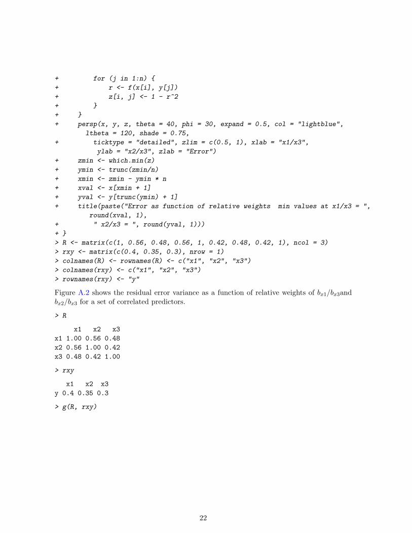
Figure A.2 shows the residual error variance as a function of relative weights of bx1/bx3andbx2/bx3 for a set of correlated predictors.

> R

x1 x2 x3x1 1.00 0.56 0.48x2 0.56 1.00 0.42x3 0.48 0.42 1.00

> rxy

x1 x2 x3y 0.4 0.35 0.3

> g(R, rxy)

22

x1/x3

−2−1

0

1

2

3

4

x2/x

3

−2

−1

0

1

2

34

Error

0.50.6

0.7

0.8

0.9

1.0

Error as function of relative weights min values at x1/x3 = 2.5 x2/x3 = 1.5

Figure A.2: Squared Error as function of misspecified beta weights. Although the optimalweights minimize the squared error, a substantial variation in the weights does not lead tovery large change in the squared error.

23

x1/x3

−2−1

0

1

2

3

4

x2/x

3

−2

−1

0

1

2

34

Error

0.50.6

0.7

0.8

0.9

1.0

Error as function of relative weights min values at x1/x3 = 1.5 x2/x3 = 1.2

Figure A.3: With orthogonal predictors, the squared error surface is somewhat better defined,although still large changes in beta weights do not lead to large changes in squared error.

With independent predictors, the response surface is somewhat steeper (Figure A.3), but stillthe squared error function does not change vary rapidly as the beta weights change. Thisphenomenon has been well discussed by Robyn Dawes and his colleagues.

x1 x2 x3x1 1 0 0x2 0 1 0x3 0 0 1

x1 x2 x3y 0.4 0.35 0.3

24