linear algebra meets lie algebra
TRANSCRIPT
Linear Algebra Meets Lie AlgebraThe Kostant-Wallach Theory
Noam ShomronBeresford Parlett
University of California, Berkeley
June, 2010
ILAS Meeting, Pisa, Italy
Gelfand-Zeitlin theory from the perspective of classical mechanics,I and IIStudies in Lie Theory, 2006.
Linear Algebra Meets Lie AlgebraThe Kostant-Wallach Theory
Noam ShomronBeresford Parlett
University of California, Berkeley
June, 2010
ILAS Meeting, Pisa, Italy
Gelfand-Zeitlin theory from the perspective of classical mechanics,I and IIStudies in Lie Theory, 2006.
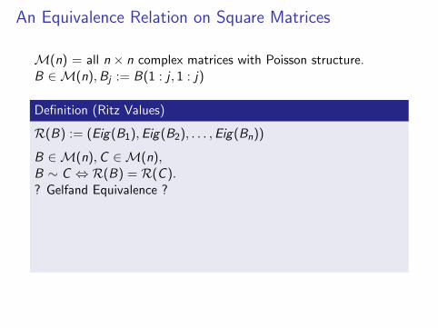
An Equivalence Relation on Square Matrices
M(n) = all n × n complex matrices with Poisson structure.B ∈M(n),Bj := B(1 : j , 1 : j)
Definition (Ritz Values)
R(B) := (Eig(B1),Eig(B2), . . . ,Eig(Bn))
B ∈M(n),C ∈M(n),B ∼ C ⇔ R(B) = R(C ).? Gelfand Equivalence ?
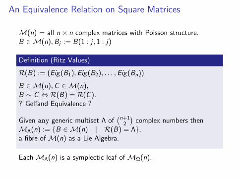
Given any generic multiset Λ of(n+1
2
)complex numbers then
MΛ(n) := B ∈M(n) | R(B) = Λ,a fibre ofM(n) as a Lie Algebra.
EachMΛ(n) is a symplectic leaf ofMΩ(n).
An Equivalence Relation on Square Matrices
M(n) = all n × n complex matrices with Poisson structure.B ∈M(n),Bj := B(1 : j , 1 : j)
Definition (Ritz Values)
R(B) := (Eig(B1),Eig(B2), . . . ,Eig(Bn))
B ∈M(n),C ∈M(n),B ∼ C ⇔ R(B) = R(C ).? Gelfand Equivalence ?
Given any generic multiset Λ of(n+1
2
)complex numbers then
MΛ(n) := B ∈M(n) | R(B) = Λ,a fibre ofM(n) as a Lie Algebra.
EachMΛ(n) is a symplectic leaf ofMΩ(n).
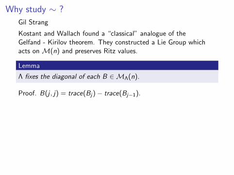
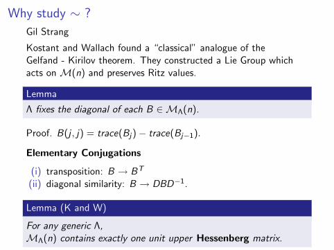
Why study ∼ ?
Gil Strang
Kostant and Wallach found a “classical” analogue of theGelfand - Kirilov theorem. They constructed a Lie Group whichacts onM(n) and preserves Ritz values.
Lemma
Λ fixes the diagonal of each B ∈MΛ(n).
Proof. B(j , j) = trace(Bj)− trace(Bj−1).
Elementary Conjugations
(i) transposition: B → BT
(ii) diagonal similarity: B → DBD−1.
Lemma (K and W)
For any generic Λ,MΛ(n) contains exactly one unit upper Hessenberg matrix.
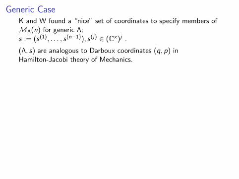
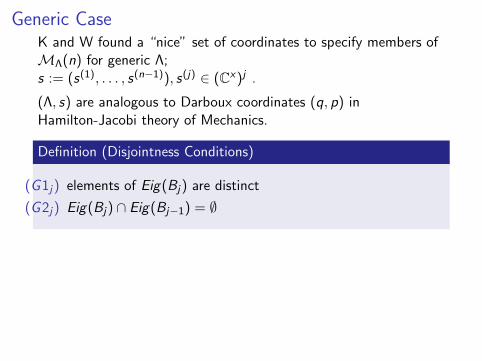
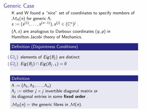
Generic CaseK and W found a “nice” set of coordinates to specify members ofMΛ(n) for generic Λ;s := (s(1), . . . , s(n−1)), s(j) ∈ (Cx)j .
(Λ, s) are analogous to Darboux coordinates (q, p) inHamilton-Jacobi theory of Mechanics.
Definition (Disjointness Conditions)
(G1j) elements of Eig(Bj) are distinct
(G2j) Eig(Bj) ∩ Eig(Bj−1) = ∅
Definition
Λ := (Λ1,Λ2, . . . ,Λn)Λj := either j × j invertible diagonal matrix orits diagonal entries in some fixed order .
MΩ(n) = the generic fibres inM(n).
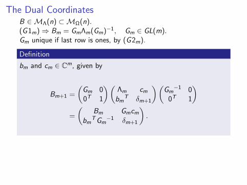
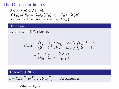
The Dual CoordinatesB ∈MΛ(n) ⊂MΩ(n).(G1m)⇒ Bm = GmΛm(Gm)−1, Gm ∈ GL(m).Gm unique if last row is ones, by (G2m).
Definition
bm and cm ∈ Cm, given by
Bm+1 =
(Gm 00T 1
) (Λm cm
bmT δm+1
) (Gm
−1 00T 1
)=
(Bm Gmcm
bmTGm
−1 δm+1
).
Theorem (BNP)
s = (1, b2T , b3
T , . . . , bn−1T ) determines B.
What is Gm ?
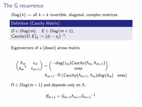
The G recurrence
Diag(k) := all k × k invertible, diagonal, complex matrices.
Definition (Cauchy Matrix)
D ∈ Diag(m), E ∈ Diag(m + 1),Cauchy(D,E )ij := (di − ej)
−1.
Eigenvectors of a (down) arrow matrix
(Λm cm
bmT δm+1
)=
(−diag(cm)Cauchy(Λm,Λm+1)
ones
)·
Λm+1 · Π(Cauchy(Λm+1,Λm)diag(bm) ones
)Π ∈ Diag(m + 1) and depends only on Λ.
Bm+1 = Gm+1Λm+1Gm+1−1.
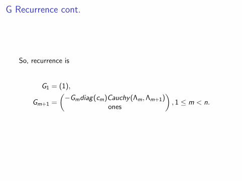
G Recurrence cont.
So, recurrence is
G1 = (1),
Gm+1 =
(−Gmdiag(cm)Cauchy(Λm,Λm+1)
ones
), 1 ≤ m < n.
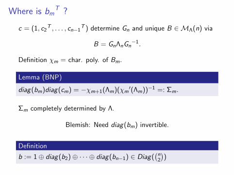
Where is bmT ?
c = (1, c2T , . . . , cn−1
T ) determine Gn and unique B ∈MΛ(n) via
B = GnΛnGn−1.
Definition χm = char. poly. of Bm.
Lemma (BNP)
diag(bm)diag(cm) = −χm+1(Λm)(χm′(Λm))−1 =: Σm.
Σm completely determined by Λ.
Blemish: Need diag(bm) invertible.
Definition
b := 1⊕ diag(b2)⊕ · · · ⊕ diag(bn−1) ∈ Diag((n2
))
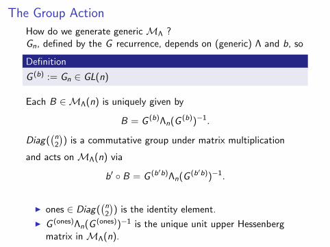
The Group Action
How do we generate generic MΛ ?Gn, defined by the G recurrence, depends on (generic) Λ and b, so
Definition
G (b) := Gn ∈ GL(n)
Each B ∈MΛ(n) is uniquely given by
B = G (b)Λn(G(b))−1.
Diag((n2
)) is a commutative group under matrix multiplication
and acts onMΛ(n) via
b′ B = G (b′b)Λn(G(b′b))−1.
I ones ∈ Diag((n2
)) is the identity element.
I G (ones)Λn(G(ones))−1 is the unique unit upper Hessenberg
matrix inMΛ(n).
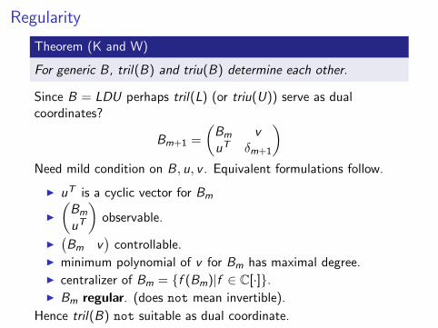
Regularity
Theorem (K and W)
For generic B, tril(B) and triu(B) determine each other.
Since B = LDU perhaps tril(L) (or triu(U)) serve as dualcoordinates?
Bm+1 =
(Bm vuT δm+1
)Need mild condition on B, u, v . Equivalent formulations follow.
I uT is a cyclic vector for Bm
I
(Bm
uT
)observable.
I(Bm v
)controllable.
I minimum polynomial of v for Bm has maximal degree.I centralizer of Bm = f (Bm)|f ∈ C[·].I Bm regular. (does not mean invertible).
Hence tril(B) not suitable as dual coordinate.
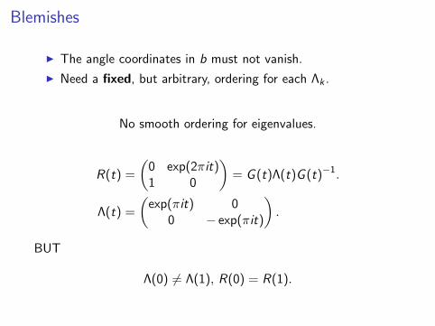
Blemishes
I The angle coordinates in b must not vanish.
I Need a fixed, but arbitrary, ordering for each Λk .
No smooth ordering for eigenvalues.
R(t) =
(0 exp(2πit)1 0
)= G (t)Λ(t)G (t)−1.
Λ(t) =
(exp(πit) 0
0 − exp(πit)
).
BUT
Λ(0) 6= Λ(1), R(0) = R(1).
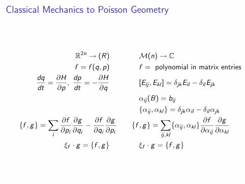
Classical Mechanics to Poisson Geometry
R2n → (R) M(n)→ Cf = f (q, p) f = polynomial in matrix entries
dq
dt=
∂H
∂p,
dp
dt= −∂H
∂q[Eij ,Ekl ] = δjkEil − δilEjk
αij(B) = bij
αij , αkl = δjkαil − δilαjk
f , g =∑
i
∂f
∂pi
∂g
∂qi− ∂f
∂qi
∂g
∂pif , g =
∑ij ,kl
αij , αkl∂f
∂αij
∂g
∂αkl
ξf · g = f , g ξf · g = f , g
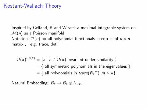
Kostant-Wallach Theory
Inspired by Gelfand, K and W seek a maximal integrable system onM(n) as a Poisson manifold.Notation. P(n) := all polynomial functionals in entries of n × nmatrix , e.g. trace, det.
P(k)GL(k) = all f ∈ P(k) invariant under similarity = all symmetric polynomials in the eigenvalues = all polynomials in trace(Bk
m),m ≤ k
Natural Embedding: Bk → Bk ⊕ In−k .
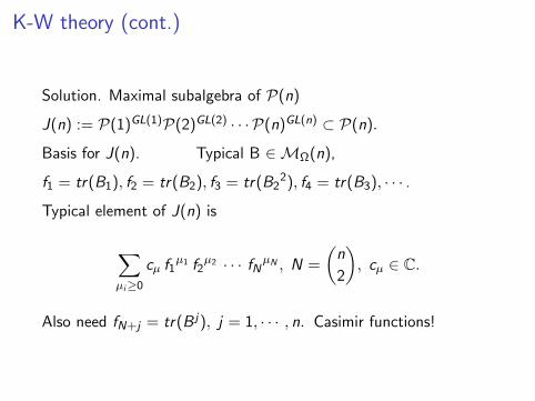
K-W theory (cont.)
Solution. Maximal subalgebra of P(n)
J(n) := P(1)GL(1)P(2)GL(2) · · · P(n)GL(n) ⊂ P(n).
Basis for J(n). Typical B ∈MΩ(n),
f1 = tr(B1), f2 = tr(B2), f3 = tr(B22), f4 = tr(B3), · · · .
Typical element of J(n) is
∑µi≥0
cµ f1µ1 f2
µ2 · · · fNµN , N =
(n
2
), cµ ∈ C.
Also need fN+j = tr(B j), j = 1, · · · , n. Casimir functions!
K-W Theory (cont.)
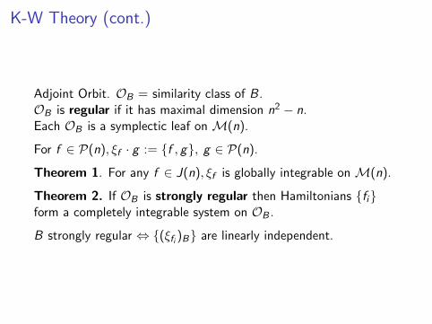
Adjoint Orbit. OB = similarity class of B.OB is regular if it has maximal dimension n2 − n.Each OB is a symplectic leaf on M(n).
For f ∈ P(n), ξf · g := f , g, g ∈ P(n).
Theorem 1. For any f ∈ J(n), ξf is globally integrable onM(n).
Theorem 2. If OB is strongly regular then Hamiltonians fiform a completely integrable system on OB .
B strongly regular ⇔ (ξfi )B are linearly independent.
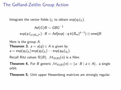
The Gelfand-Zeitlin Group Action
Integrate the vector fields ξfi to obtain exp(qiξfi ).
Ad(G )B = GBG−1
exp(q ξtr(Bm)k ) · B = Ad [exp(−q k(Bm)k−1)⊕ ones]B
Here is the group A.Theorem 3. a = a(q) ∈ A is given bya = exp(q1ξf1) exp(q2ξf2) · · · exp(qNξfN ).
Recall Ritz values R(B). MR(B)(n) is a fibre.
Theorem 4. For B generic MR(B)(n) = a · B | a ∈ A, a singleorbit.
Theorem 5. Unit upper Hessenberg matrices are strongly regular.
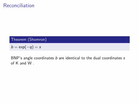
Reconciliation
Theorem (Shomron)
b = exp(−q) = s
BNP’s angle coordinates b are identical to the dual coordinates sof K and W .
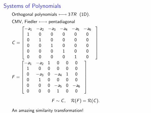
Systems of Polynomials
Orthogonal polynomials ←→ 3TR (1D).
CMV, Fiedler ←→ pentadiagonal
C =
−a1 −a2 −a3 −a4 −a5 −a6
1 0 0 0 0 00 1 0 0 0 00 0 1 0 0 00 0 0 1 0 00 0 0 0 1 0
F =
−a1 −a2 1 0 0 01 0 0 0 0 00 −a3 0 −a4 1 00 1 0 0 0 00 0 0 −a5 0 −a6
0 0 0 1 0 0
F ∼ C , R(F ) = R(C ).
An amazing similarity transformation!
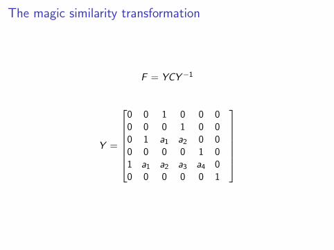
The magic similarity transformation
F = YCY−1
Y =
0 0 1 0 0 00 0 0 1 0 00 1 a1 a2 0 00 0 0 0 1 01 a1 a2 a3 a4 00 0 0 0 0 1