masterthesisreport -...

Master Thesis ReportThe impact of metallic cranial implants on proton-beamradiotherapy treatment plans for near implant located tumours

A phantom study on the physical effects and agreement between simulated treatment plans andthe resulting treatment for near implant located cranial tumours

Adam Sjögren

June 21, 2018

StudentSpring 2018Master Thesis, 30 ECTSMaster of Science in technical physics and medical physics, 300 ECTS

testing

Supervisor: Ulf Granlund ([email protected]), Department of medicalphysics, Örebro University Hospital

Examiner: Jonna Wilen ([email protected]), Department of Radiation Sciences, UmeåUniversity

Adam Sjögren ([email protected]):The impact of metallic cranial implants on proton-beam radiotherapy treatment plans for near implant located tumours, 2018.

Master’s Thesis in Engineering Physics & Medical Physics, 30.0 ECTSExamensarbete för civilingenjörsexamen i teknisk fysik, 30.0 hp

ii

Abstract

AbstractWithin the field of radiotherapy treatments of tumour diseases, the hunt for more accurate andeffective treatment methods is a continuous process. For some years ion-beam based radiother-apy, especially the proton-beam based applications, has increased in popularity and availability.The main reason behind this is the fact that ion-beam based applications make it possible tomodulate the dose after the planning target volume (PTV) defined by the radiation oncologist.This means that it becomes possible to spare tissue in another way, which might result in more ef-fective treatments, especially in the vicinity of radio sensitive organs. Ion-beam based treatmentsare however more sensitive to uncertainties in PTV position and beam range as ion-beams havea fixed range depending on target media and initial energy, as opposed to the conventional x-raybeams that do not really have a defined range. Instead their intensity decreases exponentiallyat a rate dependent of the initial energy and target media. Therefore density heterogeneitiesresult in uncertainties in the planned treatments. As the plans normally are created using a CT-images, for which metallic implants can yield increased heterogeneities both from the implantsthemselves and so called metal artifacts (distortions in the images caused by different processesas the X-rays used in image acquisition goes through metals). Metallic implants affects the ac-curacy of a treatment, and therefore also the related risks, so it is important to have an ideaof the magnitude of the impact. Therefore the aim of this study is to estimate the impact ona proton-beam based treatment plan for six cranial implants. These were one Ti-mesh implant,one temporal plate implant, one burr-hole cover implant and three craniofix implants of differentsizes, which all are commonly seen at the Skandion clinic. Also the ability of the treatmentplanning system (TPS), used at the clinic, to simulate the effects on the plans caused by theimplants is to be studied. From this result it should be estimated if the margins and practicesin place at the clinic, for when it is required to aim the beam through the implant, are sufficientor if they should be changed.

This study consisted of one test on the range shift effects and one test on the lateral dose dis-tribution changes, with one preparational test in the form of a calibration of Gafchromic EBT3films. The range shift test was performed on three of the implants, excluding the three craniofiximplants using a water phantom and a treatment plan created to represent a standard treatmentin the cranial area. The lateral dose distribution change test was performed as a solid phantomstudy using radiochromic film, for two treatment plans (one where the PTV was located 2 cmbelow surface, for all implants, and one where it was located at the surface, only for the Ti-meshand the temporal plate). The results of both tests were compared to simulations performed inthe Eclipse treatment planing system (TPS) available at Skandion.

The result of the range shift test showed a maximum range shift of −1.03(1) mm, for the burr-holecover implant, and as the related Eclipse simulations showed a maximal shift of −0.17(1) mmthere was a clear problem with the simulation. However, this might not be because of the TPSbut due to errors in the CT-image reconstruction, such as, for example, geometrical errors in therepresentation of the implants. As the margin applied for a similar situation at the Skandionclinic (in order to correct for several uncertainty factors) is 4.2 mm there might be a need toincrease this margin depending on the situation.

For the lateral distribution effects no definite results were found as the change varied in magni-tude, even if it tended to manifest as a decreasing dose for the first plan and a increasing dosefor the second. It was therefore concluded that further studies are needed before anything clearcan be said.

iii

Sammanfattning på svenska

Sammanfattning på svenskaInom cancervården går utvecklingen konstant framåt och sökandet efter nya, effektivare metoderinom området extern radioterapi är inget undantag. Inom extern radioterapi använder mansig utav joniserande strålar (strålar som genom att överföra energi till molekyler joniserar demvilket bryter isär molekylen) som riktas genom en patient och koncentreras i ett lokalt target vidtumören. Genom att deposera tillräckligt mycket dos (ett mått av energi per massa) till tumörenhoppas man, inom radioterapi döda samtliga cancerceller och på så vis lyckas behandla cancern,men man måste samtidigt vara försiktig med att inte deposera för mycket dos i frisk vävnad.

Det konventionella valet vid extern radioterapi är att använda sig av fotonstrålar inom röntgen-spektrat, med våglängder mellan 10 pm och 1 nm, men de senaste åren har metoder baserade påladdade partiklar, främst protoner, blivit alltmer tillgängliga. Den stora skillnaden mellan fotonoch partikel-baserade strålar är hur de deposerar dos. Medans fotonstrålar tränger igenom helapatientens kropp och deposerar avtagande mängd dos på väger tränger laddade partiklar barain till ett specifikt djup, beroende av dess initiella energi, och deposerar majoriteten av dosen påslutet. Detta innebär att metoder baserade på strålar av laddade partiklar gör det möjligt attmodulera behandlingen så att mer frisk vävnad blir helt skonad från deposerad dos, vilket gördessa metoder extra lämpade för behandling av cancer i närheten av strålkänslig vävnad. Dettabetende med ett specifikt djup gör samtidigt dessa metoder betydligt känsligare för variationeri patientens densitet, och framför allt om metalliska implantat finns i närheten av tumören. Föratt planera en behandling använder man sig av ett CT-underlag (en slags 3D röntgen-bild) ochmetall resulterar i vad man kallar för metallartefakter (en typ av störningar), dessa resulterar iatt patientens anatomi, och metallens storlek, missvisas. Detta medför att det finns en risk atten del av tumören inte får tillräckligt mycket dos för att behandlingen skall lyckas eller att frisknärliggande vävnad får skadligt hög dos. Det är därför viktigt att ta hänsyn till detta då manär tvungen att rikta strålarna genom metall.

I denna studien har man kollat på hur 6 titan-baserade kraniella implantat påverkar protonbe-handlings planer vid Skandion-kliniken i Uppsala, den enda kliniken i sverige där protonbaseradradioterapi är möjlig. Detta har utförts genom en fantom-studie (studie där man använt olika ma-terial för att simulera en behandling) där man undersökt hur protonernas räckvidd påverkats avatt implantaten placerats i fältet. Samt hur dosfördelningen i ett plan på olika djup påverkatsför en plan där target låg på ett djup av 2 cm och en där target låg i ytan. Resultaten haräven jämförts med simuleringar utförda i klinikens planerings programm för att studera hur välde fysiska förändringarna har simulerats vid planeringen, vilket ger en indikation om huruvidamarginalerna som redan läggs till vid kliniken är tillräckliga eller om de behöver ses över.

Resultaten visade att det var betydande skillnader mellan simuleringarna utav räckviddenspåverkan och de fysiska mätningarna då simuleringarna till hög grad underskattade effekten.Det noterades dock att detta kan ha grund hur väl CT-underlagen representerade verklighetenoch att man bör studera detta närmare innan slutgiltig slutsats kan fastslås, men det kan, förvissa fall, vara aktuellt att se över marginalerna som appliceras vid kliniken. När det gälldedosfördelningen i de olika planen visade en dosminsknings trend för planen där target låg litedjupare och en dosöknings trend på den ytliga planen, men det gick inte att bestämma nån klarstorlek på grund av varierande magnitud för de olika djupen och implantaten, så det fastslogsatt vidare studier krävs innan slutgiltig slutsats kan fastslås.

iv

Acknowledgements

AcknowledgementsFirst I would like to direct the sincerest gratitude towards my supervisor, Ulf Granlund, at Uni-versitetssjukhuset Örebro who introduced me to the field and has done a great work guiding meon the path of this work.

A continued thank you to the personnel at the Skandion clinic, especially Karin Andersson,Christina Vallhagen Dahlgren and Liliana Stolarczyk for their great support with the practicalwork during the tests and for letting me take part of their wast expertise in the field.

A great deal of gratitude is directed towards Michael Gubanski and Petra Witt Nyström whosupplied the study with the implants, without which this work would have been impossible toperform.

Thank you to the rest of the personnel at the department for medical physics at UniversitetssjukhusetÖrebro for taking me in and for the support. You all made this time great.

Further on I would like to thank my parents and grand parents, both paternal and maternal,for the different levels of support provided, while not understanding most of what I was talkingabout. And also thanks to my brothers for supporting me ”in their own special way”.

Lastly I wold like to thank my fellow students and friends both near and far who lightened upthe days when the pressure of the studies grew a bit heavy. And that from time to time putsome light in my days by, for example, trying to force me into saying something fun.

v

Nomenclature and abbreviations


A short description of some of the words and abbreviations used in this thesis.

CT Computed Tomography, a method used to creating 3D-images using a x-ray setup that rotates around the objectbeing imaged, usually a patient.

Radiotherapy A term used to group medical treatments in which ionizingradiation is used (not diagnostics).

Gy Gray, a unit used to describe the amount of energy absorbedin a tissue due to radiation, defined as one joule per kilogramof tissue.

DSB Double Strand Break, describes a damage to a DNA-molecule where both strands of the DNA is damaged ina localized area, often resulting in a full break of the DNA-molecule. As it is difficult for the cell to repair a DSB itoften results in the death of the cell.

CTV Clinical Target Volume, a volume deined within the patient,by a radiation oncologist, in which the tumour and possiblemicroscopic cancerous spread is located.

PTV Planning Target Volume, defined by the radiation oncolo-gist as the CTV + an extra margin in order to correct foruncertainties in tumour position due to, for example, er-rors in day to day setup and organ movements. The PTVis used during treatment planning in order to make surethat the tumour absorbs a high enough dose to guaranteesuccessful treatment.

LET Linear Energy transfer, the local transfer of energy per unittrack length traveled by a particle within a media.

BP Bragg peak, the distinctive peak which is found at the end ofa Bragg curve, which in turn is the characteristic percentagedepth-dose curve for protons and larger charged particles.

SOBP Spread Out Bragg Peak, a plateau received through the mod-ulation of particle energy resulting in a plateau of multipleBragg peaks at different depths, making it possible to mod-ulate the deposited dose after the PTV.

TPS Treatment Planning System, a software used to plan, andsimulate, a radiotherapeutic treatment.

MARS Metal Artifact Reduction Software, a type of software usedto reduce image distortions in a CT image resulting fromthe presence of metals in the depicted patient.

iMAR Iterative Metal Artifact Reduction, the MARS supplied bySiemens Healthineers for their products.

vi


WET Water Equivalent Thickness, the thickness of water thathas the same properties as a slab of a certain thickness andmaterial from a radio-physical point of view.

Mass stopping power The amount of energy lost per unit length travelled by acertain particle with a certain initial energy through a cer-tain material with a certain density due to interactions withmatter.

R50 Range 50 %, the range from the surface into a target towhich a minimum of 50 % of the maximum dose has beenabsorbed. A value often used when comparing differenttreatment plans.

Gafchromic EBT3 A type of radiochromic film (radiation activated self devel-oping film used as a radiation detector).

Plane-parallel ionizationchamber

A radiation detector consisting of two conductive platesthat measures dose through the collection and measurementof the charge created through ionization of air between thetwo plates within a waterproof shell.

vii

Contents

Contents

Abstract iii

Sammanfattning på svenska iv

Acknowledgements v

Nomenclature and abbreviations vi

1 Introduction 11.1 Purpose . . . . . . . . . . . . . . . . . . . . . . . . . . . . . . . . . . . . . . . . . . . . . . 11.2 Disposition . . . . . . . . . . . . . . . . . . . . . . . . . . . . . . . . . . . . . . . . . . . . 1

2 Background and theory 32.1 Radiotherapy . . . . . . . . . . . . . . . . . . . . . . . . . . . . . . . . . . . . . . . . . . . 3

2.1.1 The basics of radiotherapy . . . . . . . . . . . . . . . . . . . . . . . . . . . . . . . . 32.1.2 Photon- versus particle-beams . . . . . . . . . . . . . . . . . . . . . . . . . . . . . . 4

2.2 The problem with metallic implants in radiotherapy . . . . . . . . . . . . . . . . . . . . . 52.3 The connection between water and tissue from a radiophysical viewpoint . . . . . . . . . . 72.4 Range shift and R50 . . . . . . . . . . . . . . . . . . . . . . . . . . . . . . . . . . . . . . . 72.5 The Skandion clinic . . . . . . . . . . . . . . . . . . . . . . . . . . . . . . . . . . . . . . . . 8

3 Material and software used in the study 93.1 The implants . . . . . . . . . . . . . . . . . . . . . . . . . . . . . . . . . . . . . . . . . . . 9

3.1.1 Titanium mesh implants (implant 1 and 2) . . . . . . . . . . . . . . . . . . . . . . . 93.1.2 Burr-hole cover (implant 3) . . . . . . . . . . . . . . . . . . . . . . . . . . . . . . . 93.1.3 Craniofix (implant 4-6) . . . . . . . . . . . . . . . . . . . . . . . . . . . . . . . . . . 10

3.2 Radiochromic film . . . . . . . . . . . . . . . . . . . . . . . . . . . . . . . . . . . . . . . . 113.2.1 General information regarding radiochromic films . . . . . . . . . . . . . . . . . . . 113.2.2 The Gafchromic EBT3 radiochromic film . . . . . . . . . . . . . . . . . . . . . . . . 12

3.3 Blue Phantom2 . . . . . . . . . . . . . . . . . . . . . . . . . . . . . . . . . . . . . . . . . . 133.4 Solid phantom material . . . . . . . . . . . . . . . . . . . . . . . . . . . . . . . . . . . . . . 133.5 Other equipment and software used . . . . . . . . . . . . . . . . . . . . . . . . . . . . . . . 14

4 Experimental methods 154.1 Calibration of the EBT3 films . . . . . . . . . . . . . . . . . . . . . . . . . . . . . . . . . . 154.2 Range effects . . . . . . . . . . . . . . . . . . . . . . . . . . . . . . . . . . . . . . . . . . . 164.3 Lateral dose distribution . . . . . . . . . . . . . . . . . . . . . . . . . . . . . . . . . . . . . 17

5 Results 205.1 Calibration . . . . . . . . . . . . . . . . . . . . . . . . . . . . . . . . . . . . . . . . . . . . 205.2 The range effects . . . . . . . . . . . . . . . . . . . . . . . . . . . . . . . . . . . . . . . . . 21

5.2.1 Including bone equivalent plates . . . . . . . . . . . . . . . . . . . . . . . . . . . . . 215.2.2 Excluding bone equivalent plates . . . . . . . . . . . . . . . . . . . . . . . . . . . . 22

5.3 Lateral dose distribution . . . . . . . . . . . . . . . . . . . . . . . . . . . . . . . . . . . . . 235.3.1 Deeper setup . . . . . . . . . . . . . . . . . . . . . . . . . . . . . . . . . . . . . . . 235.3.2 Surficial setup . . . . . . . . . . . . . . . . . . . . . . . . . . . . . . . . . . . . . . . 24

6 Discussion 266.1 Calibration . . . . . . . . . . . . . . . . . . . . . . . . . . . . . . . . . . . . . . . . . . . . 266.2 Range effects . . . . . . . . . . . . . . . . . . . . . . . . . . . . . . . . . . . . . . . . . . . 266.3 Lateral dose distribution . . . . . . . . . . . . . . . . . . . . . . . . . . . . . . . . . . . . . 27

viii

Contents

7 Conclusion 29

8 References 30

A EBT3 film calibration data 32

B Range effects including bone equivalent plates, additional images and data 34B.1 implant 1 . . . . . . . . . . . . . . . . . . . . . . . . . . . . . . . . . . . . . . . . . . . . . 35B.2 implant 2 . . . . . . . . . . . . . . . . . . . . . . . . . . . . . . . . . . . . . . . . . . . . . 36B.3 implant 3 . . . . . . . . . . . . . . . . . . . . . . . . . . . . . . . . . . . . . . . . . . . . . 37

C Range effects excluding bone equivalent plates, additional images and data 38C.1 implant 1 . . . . . . . . . . . . . . . . . . . . . . . . . . . . . . . . . . . . . . . . . . . . . 39C.2 implant 2 . . . . . . . . . . . . . . . . . . . . . . . . . . . . . . . . . . . . . . . . . . . . . 39

D Lateral dose distribution, additional images and data 41D.1 The reference (deep setup) . . . . . . . . . . . . . . . . . . . . . . . . . . . . . . . . . . . . 41D.2 Implant 1 (deep setup) . . . . . . . . . . . . . . . . . . . . . . . . . . . . . . . . . . . . . . 42D.3 Implant 2 (deep setup) . . . . . . . . . . . . . . . . . . . . . . . . . . . . . . . . . . . . . . 43D.4 Implant 3 (deep setup) . . . . . . . . . . . . . . . . . . . . . . . . . . . . . . . . . . . . . . 44D.5 Implant 4 (deep setup) . . . . . . . . . . . . . . . . . . . . . . . . . . . . . . . . . . . . . . 45D.6 Implant 5 (deep setup) . . . . . . . . . . . . . . . . . . . . . . . . . . . . . . . . . . . . . . 46D.7 Implant 6 (deep setup) . . . . . . . . . . . . . . . . . . . . . . . . . . . . . . . . . . . . . . 47D.8 The reference, surface target . . . . . . . . . . . . . . . . . . . . . . . . . . . . . . . . . . . 48D.9 Implant 1 (surface setup) . . . . . . . . . . . . . . . . . . . . . . . . . . . . . . . . . . . . 48D.10 Implant 2 (surface setup) . . . . . . . . . . . . . . . . . . . . . . . . . . . . . . . . . . . . 49

ix

1. Introduction

1 IntroductionThe fact that cancer is a terrible diagnose for anyone to receive is widely known, but most peopleprobably only have a minimal knowledge about how different forms of cancer are treated. Some of themost common treatments are the different forms of radiotherapy (the use of different forms of ionizingradiation) in which the external group (using beams of either photons or charged particles) are the mostcommon one. The idea behind all radiotherapy can be described in the sentence ”The deliverance of theright dose to the right target volume”. This means that it is important that the right amount of energyis delivered to the cancer and as little as possible to the healthy tissue surrounding it as the radiationitself can result in severe side effects, such as radiation-induced cancer later in life or the loss of functionin the irradiated organs. This means that it is highly important that the accuracy of the treatment issufficient as the target is to be given a high enough dose to kill all the cancerous cells in order for thetreatment to be successful.

The conventional method for external treatments are the use of photon-beams, where beams of photonsare sent through the body with exponentially decreasing energy-deposition. Using several beams withdifferent angles through the body the dose deposited can be modelled so that the target receives theprescribed dose and the healthy tissue a lower. Charged particle beam methods, like using proton beams,work a bit different as there are clear differences in the way that photons and charged particles deliverenergy. Charged particles instead deliver a lower, rather constant, dose as it travels through the tissue,until it reaches a certain range, depending on its initial energy, where almost all is deposited to a singlepoint. This means that while photons deliver dose through the whole body charged particles only de-liver dose to a certain depth. The treatment plan is designed so that the initial energies of the chargedparticles results in that the target area receives the prescribed dose. There are, however, some increasedrisks with the use of charged particle beams though. The fact that these methods only deliver dose to acertain depth means that the treatments are sensitive to shifts in the range of the charged particles thatcan come from several sources. Generally a denser material allows for a shorter range as it is dependenton both the initial energy of the particle and the material properties. So if the body of the patient is notmodelled sufficiently well by the CT image used in the planning of the treatment, the result might bethat parts of the target is given too low dose and the cancer survive or the healthy tissue can be givendoses that are so high that the severe side effects earlier mentioned might occur. This is a well knownproblem when the target is in the close vicinity of metallic implants as metals creates so called artifactsin the CT-images that misrepresents the size of the implants and the anatomical build of the patient.There are different ways to tackle these problems and treatment-planning systems are designed to takeit into consideration to some extent. But the effects of different implants and how the treatment plansmirrors the real outcome of the treatment are not studied sufficiently enough, so that is what this studylooks into.

1.1 PurposeThe purpose of this study is to investigate how six of the cranial implants more commonly seen atthe Skandion clinic in Uppsala, Sweden, effects proton-beam radiotherapy treatments of near implantlocated tumour diseases. The ability of the software, available at the clinic, to simulate these effects willalso be studied in order to estimate if the margins and practices already at place are sufficient, or if theyneed to be changed for situations were it is required to aim the beams through the implants for somereason.

1.2 DispositionIn Sec. 2 and 3 the relevant theory and information about the equipment used in the study is presented.Within Sec. 4 the methods of the study are described. The results are presented in Sec. 5 with additional

1

1. Introduction

information that can help with the understanding of the results presented within appendices A to D. InSec. 6 a discussion regarding the results is presented as a base for the conclusion presented in Sec. 7.

2

2. Background and theory

2 Background and theory

2.1 RadiotherapyRadiotherapy is a word used when speaking about medical treatments using radiation and the termincludes several different methods used, both externally and internally. In internal radiotherapy methodsthe radiation is delivered by a source that is inserted into the patients body. This might be in the formof liquids, used in nuclear-medicine therapy applications, or solid sources, used in brachy-therapy. Theexternal therapy methods are methods were beams of either photons or charged particles are used fromthe outside. The external methods are more common and the methods are constantly evolving.

2.1.1 The basics of radiotherapy

The aim with all forms of radiotherapy is to deposit the right dose to the right volume and in medicalphysics three quantities of dose are defined, absorbed dose, equivalent dose and effective dose. In radio-therapy one usually only use the absorbed dose, which is defined as

D = dE

dm(1)

where dE is the mean energy deposited to matter of mass dm [1] due to ionizing radiation. Absorbeddose is given in the unit gray (written as Gy) and one gray is defined as one joule per kilogram of tissue.

The main process searched after in successful radiotherapy treatments is the creation of so called double-strand breaks (DSB) which is a damage on the DNA sequence due to radiation where both strands arebroken at a close distance due to the ionization of DNA-molecules by ionizing radiation [2]. DSB damageis hard for the cells to repair and the result is that the cells can not go through the mitosis cycle andeventually the cells dies. So the aim of radiotherapy treatments is to deposit enough dose to the so calledclinical target volume (CTV). A CTV is defined as a volume containing the cancerous tumour with amargin containing possible microscopic cancer spread [3]. If the CTV does not receive enough dose somecancerous cells might survive, leading to a failed treatment as the cancer might return from just one cell.In order to account for uncertainties in CTV position, for example due to daily setup uncertainty andorgan movements, another volume is defined called planning target volume (PTV). The PTV is a volumecontaining the CTV and with a margin depending on the location of the tumour and the surroundinganatomy [3].

However, radiotherapy can also result in severe side effects when healthy tissues receives enough dose,for example radiation induced cancer up to several years later in life and decreased function of irradiatedorgans. This means that it is highly important that the treatment is given with a high enough accuracyso that the PTV gets enough dose and the surrounding, healthy tissue is spared as much as possible.So one of the most important aspects in radiotherapy is the accuracy. This can be solved in severaldifferent ways. In internal radiotherapy this has been done by taking the radiation source to the tumour.For nuclear-medicine radioactive isotopes of different substances that are naturally absorbed by the sicktissues are used. In brachy-therapy one inserts solid metallic sources in the direct vicinity of the tumour.Through this only the area of the tumour absorbs dose. In external therapy beams of photons or chargedparticles are used and here the problem is solved through the use of several beam directions resultingin that beams are sent through the patient with different directions all aimed towards the PTV. Thisresults in that the tissues on the beams way to and from the PTV will receive some dose but lower asthe dose from the different beams are collected in the PTV, so when more beams are used a lower doseis absorbed by healthy tissue.

3


2.1.2 Photon- versus particle-beams

The conventional choice of beam type in external radiotherapy is photon beams, but particle based appli-cations are increasing in popularity. Photon- and particle-beams have significantly different propertiesdue to the nature of the processes through which they interact with matter, which results in that theydeposit energy in different ways.

Photon-beams used in radiotherapy are in the X-ray range of the electromagnetic spectra and thus cantravel through the human body. The beams intensity decreases exponentially as the distance traveledin a certain media increases. This can be seen in a percentage depth-dose curve, as in Fig. 1, whichdepict the amount of dose delivered by a certain ionizing beam at a certain energy as it goes througha specified media. However, this decrease in dose only takes place after a initial increase in the smallbuild-up region, due to initial increase of photon-density as a result of scattering in the media. The dosefrom photon-beams are mainly deposited through the absorption of some or all of the energy of a singlephoton by an atom.

For charged particles the processes are quite different as the dose is instead deposited through differentcharge and particle interaction. Larger charged particles interact with more particles per unit distancetraveled and also the charge and initial energy have a great impact on the dose deposition. For chargedparticles the concept of linear energy transfer (LET), defined as the local transfer of energy per unittrack length, is applied. That is the average collision energy loss dE up to a maximum energy loss ∆Efor a distance dl, defined as

LET =(

dE

dl

)∆E

. (2)

Basically, the lower the kinetic energy of a particle is the higher the probability of interaction is. Thismeans that the LET increases with decreasing kinetic energy of the particle. Following this the percent-age depth-dose curves of particle beams usually takes a rather distinct shape, especially for the heavycharged particles. For these heavy charged particles (protons and all charged particles larger than that)the percentage depth-dose curve is in the shape of a so called Bragg curve with the distinctive Braggpeak (BP). The distinctive shape of the BP is, as explained by Frank Herbert Attix in Introductionto Radiological Physics and Radiation Dosimetry [4], a consequence of the dependence of the kineticenergy for a heavy particle at lower energies when it comes to the probability of interactions. A heavyparticle will deposit half its initial energy while traveling a distance x and the remaining half will thenbe deposited while traveling only a distance ∼= x

3 . a typical example of this can be seen in Fig. 1. Thismeans that a lower amount of dose is deposited until a certain, predictable, depth is reached where themajority of the dose is deposited. The BP behaviour of larger charged particles is a large part of thereason to why particle beams are increasing in popularity. The fact that dose is deposited on the waytowards the target and in the target itself, but practically no dose after the target make it possible tospare more healthy tissue using charged particles instead of photons which deposit dose even after thetarget [5]. This is helpful in cases where radiation sensitive organs (clinically called organs at risk orOAR) are close to the PTV. Also, since the position range of the particles, and through that the positionof the BP, are dependent of the initial energy of the particle-beam it is possible to shape a so calledspread out Bragg peak (SOBP) by varying the initial energy, see Fig. 1. The use of a SOBP makes itpossible to creat a plateau of a certain dose that can be modeled to cover the PTV, making it possible tohave deposit a therapy dose to the PTV and only a relatively low dose to the healthy tissue on the wayin and practically no dose to the rest of the tissue, except for a small amount of possibly scattered protons.

4


Figure 1 – A simple presentation of the depth-dose behaviour of photons and protons with theBragg peak of a single-energy proton beam clearly visible at the end of the SOBP-plateau. Figureheavily based upon an image found in the publication Proton Beam Therapy for Non-Small CellLung Cancer: Current Clinical Evidence and Future Directions by Abigail T. Berman et al [6].

2.2 The problem with metallic implants in radiotherapy

The first part of any radiotherapy treatment is the creation of the treatment plans which are based oneither a MR- (magnetic resonance) or, much more commonly, CT-scan (computed tomography) of thepatient. This means that the quality of the treatment is highly dependent on the quality of the image-basis used in planning as the anatomical structure of the patient is used to calculate the deposited doseto different volumes. If the planing basis does not represent the patients anatomy well enough, the planwill contain larger uncertainties that needs to be corrected for.

It is well known that metallic objects are a common source of so called artifacts (distortions in the image)in CT- and MR-scans, but in this work focus lies upon the CT-based therapy. The reason behind theproblems with metals is the fact that medias of higher atomic number are ”denser” when it comes toradiation and therefore the X-rays used in CT can not pass through metals as easily, and what builds upthe CT-image is the amount of radiation that passes through the media to the detectors on the oppositeside. The so artifacts resulting from metals are commonly called metal streak artifacts and are often seenas clear black and white streaks beaming out from the metallic structure, sometimes making it impossibleto distinguish any anatomical structures. The intensity of a tissue in a CT-image is directly correlatedto its radiation density and it is used later by the treatment planning system (TPS) to calculate andsimulate the treatment plan, so it is clear that these effects have a great impact on the treatment andneed to be accounted for. Different metal artifact reducing software’s are developed by the companiesthat produce CT-scanners, such as O-MAR (Metal Artifact Reduction for Orthopedic implants) fromPhilips [7] or iMAR (Iterative Metal Artifact Reduction) from Siemens Healthineers [8], that have beenseen to improve the image quality (for most but not all cases). An example of the metal artifact streakproblem can be seen in Fig. 2.

5


(a)(b)

Figure 2 – Images demonstrating the problems with metallic streak artifacts. In (a) the metallicstreak artifacts resulting from amalgam dental repairs, as can be seen it is hard to distinguish anyanatomical data of the jaw and teeth area. In (b) the same image is shown after being enhancedby a metal artifact reducing software. Images from University hospital of Örebro.

Even if metal artifact reducing softwares can increase the quality of a CT-image to a great degree therewill still be uncertainties in the image that will need to be accounted for. There will be a certain uncer-tainty in the density of reconstructed tissue data and some smaller structures might be missing fully sothe treatment plans might differ from the resulting treatment at a significant level. This means that themargin used to correct the plan for uncertainties from other sources such as intestinal movements andchange of tumour size throughout the treatment might need to be increased depending on what kind ofimplant is located in the area. Also it is required to know how large the effects are in order to decide ifit is possible to aim the beam through the implant or if it should be avoided.

There is however much more to be studied when it comes to the impact of metallic implants on treatmentplans. While several studies have been performed regarding the impact of metallic objects on treatments,such as the publications by Isabelle Dietlicher et al[9], Yincui Jia et al [10] and Joost M. Verburg et al[11], only a few studies have been performed regarding the cranial area. One of those is the study Theeffects of titanium mesh on passive-scattering proton dose of Haibo Lin et al [5] where the impact of a0.6 mm titanium mesh implant, with a metal-to-hole ratio of 0.85, on a plan in a certain patient casewas studied. For the studied case their group saw dosimetric impacts below 1 % and a range reductionof less than 0.5 mm, however they noted that an similar analysis might bee needed for each individualcase. As there are several other kinds of metallic cranial implants available, with varying thickness andstructure this study will look upon some implants that are commonly encountered at the Skandion clinicin Uppsala, Sweden, in order to determine how treatment plans should be made when those implantsare found in the vicinity of treatment areas.

The impact of an implant on a treatment plan is dependent of the material and structure of the implant.It is critical that the implants surface is constructed by a biomedical material, which is a material thatis wall suited functionally for the task and at the same time is as compatible as possible with humantissue. For many of the newer metallic implants titanium and titanium alloy based materials are the

6


material of choice due to the high bio-compatibility of those materials, and the fact that they producerelatively less artifacts, especially for smaller implants. Many of the cranial implants need to be able toprotect the brain from impacts as they are often used to either used to replace pieces of cranial boneremoved during neurosurgery or to hold those pieces in place after surgery. This means that metal is awell suited choice for implants due to their rigidity.

2.3 The connection between water and tissue from a radiophysicalviewpoint

The human body mostly consists of water and about 50 %-60 % of an adults total weight is water, addingto that is the fact that most of the human organs consist of between 70 %-80 % water (notable exceptionsto this is bone, 20 %, and fat, 10 %) [12]. This means that most of the human body can be approximatedto water in most radiophysical situations making it easier to perform measurements and simulationsusing water instead of real tissues. This also makes it possible to produce sufficiently accurate calcu-lations using tabulated values without the need to consider anatomical differences between individualsand different tissues.

It should however be noted that no tissue is exactly water equivalent. Which for most situations is nota critical problem, but in some cases there is a need to take the effects into consideration. In some casesit is impossible to perform certain measurements with regular water due to several possible reasons, forexample when using solid phantoms or measurement equipment that can be damaged by water. In orderto take this into consideration most phantom materials have a so called WET value, which stands forwater equivalent thickness and describes the ratio between the thickness of the material and the thicknessof a piece of liquid water that has the same properties in a radio-physical viewpoint. WET is defined(by Rui Zhang and Wayne D Newhauser [13]) as

W ET = tw ≈ tmρmSm

ρwSw

, (3)

where t is the thickness, rho is the mass density and S is the mean proton mass stopping power and thesubindexes m and w denotes if the value is related to the relevant material (m) or water (w). S in turnis defined as

S =´

ESdE´

EdE

, (4)

where E is the energy of a proton and S is the proton mass stopping power related to a certain energy.

2.4 Range shift and R50

Due to the fact that a proton beam of a certain energy have a fixed range depending on the targetmedias density any heterogeneities introduced to the media will affect the range of the beam. This effectis simply called range shift and is for obvious reasons significant when it comes to proton beam basedradiotherapy as it, at a great magnitude, affects the accuracy of the treatment, so it is important tocorrect for these effects in order to maximize the treatment outcome.

In the publication A semi-empirical model for the therapeutic range shift estimation caused by inhomo-geneities in proton beam therapy by Moskvin et al [14] a simple model is presented that makes it possibleto calculate an estimation of the maximum range shift introduced by a object in the common protonbeam energy range for radiotherapy purposes. This model, defined as

7


∆(tM , Z) = tM [ρM (1.192 − 0.158ln(Z)) − 1] (5)calculates the water equivalent range shift ∆x coming from an object of thickness tM and density ρM

with atomic number Z.

In dosimetry radiotherapy it is often helpful to talk about well defined entities and as the total rangeoften is hard to define the term RN is used, which is defined as the range into a target volume thatreceives at least N% of the maximum dose. In this study this range is defined as the range in the targetthat absorbs a dose equal to at least half the maximum absorbed dose, which is R50.

2.5 The Skandion clinicThe Skandion clinic in Uppsala, Sweden, is the first clinic dedicated towards proton-beam radiotherapyin Scandinavia. The clinic is a national project driven together by the 7 counties in Sweden that containsuniversity classed hospitals, through komunalförbundet avancerad strålbehandling. The main equipmentat the location is the model Proteus PLUS cyclotron (IBA worldwide) which supplies the clinic withproton beams of up to 230 MeV. In each treatment room the beam is distributed via a specialized nozzlewhich is moved around the patient by a so called gantry, which is not visible from the room itself, seeFig. 3. At this moment there are two active treatment rooms, with the space to install a third, and aroom containing a nozzle without a gantry used purely for research.

The clinic is driven using the principle of distributed competence, the medical responsibility throughoutthe whole treatment is held by the patients home hospital and only the actual treatment is performedat Skandion. The patient is examined and prepared at the hospital where all fixation equipment andtreatment plans are prepared. Only after all is prepared and a treatment plan has been approved byboth the hospital and the group at Skandion the patient is sent to Skandion to receive treatment. Afterthe treatment is done the follow up work and controls are performed in place at the hospital. Fromthis follows that the results of this study is relevant to all hospitals connected to the Skandion clincas the work with the plans and preparations is where one need to take the effects of the implants intoconsideration.

Figure 3 – One of the treatment rooms at The Skandion clinic with the nozzle clearly visibleover the patient coach, the gantry is separated from the room via the wall but the size of it canbe imagined due to the fact that the cylindrical area is within it.

8

3. Material and software used in the study

3 Material and software used in the studyWithin this section the materials used within this study are presented.

3.1 The implantsWhat follows here is a presentation of the six implants used within the study.

3.1.1 Titanium mesh implants (implant 1 and 2)

In this study two types of titanium mesh implants were used, one 9 cm × 9 cm Ti-mesh implant (calledimplant 1 in this study) with a thickness of 0.3 mm and one temporal plate implant (called implant2 in this study) with a thickness of 0.4 mm, both shown in Fig. 4 and 5. Titanium mesh implants areusually used to replace pieces of bone removed during brain surgery and are screwed in place over thehole in the cranium using small, self drilling, titanium screws, which means that it often might be hardto avoid beaming through the implant. However, as was seen in the work of Lin et al the effect of a0.6 mm titanium mesh implant was quite small so it is expected that the effect of the thinner mesh islower than that as the implant used in this study is only half as thick as the one used in their.

Figure 4 – The titanium mesh implant(implant 1) used in the tests

Figure 5 – The titanium temporal plateimplant (implant 2), with a piece of tapeused to mark position directors.

3.1.2 Burr-hole cover (implant 3)

The burr-hole cover implant used in this study (called implant 3) was a titanium based circular platewith a diameter of 17 mm and a thickness of 0.5 mm, see Fig. 6, which as the name implies is used tocover a burr-hole made in the cranial bone. The implant is fixated onto the cranium using small selfdrilling titanium screws of the same kind as the ones used for the titanium mesh implants, where thesmaller peripheral rings on the implant is used as anchor points for the screws. There are also somemodels with a different structure specially designed to allow for a shunt to be inserted without the needfor additional holes, but that type of implant will not be used in this study.

9


Figure 6 – The Burr-hole cover implant (implant 3), used in the study. In the upper right cornerthe kind of Ti screws, used to attach the burr-hole cover and Ti-mesh implants to the cranial bone,can be seen.

3.1.3 Craniofix (implant 4-6)

Craniofix implants are constructed as two parallel Ti-based plates connected in the center by a ribbedrod. They are used to re-fixate the pieces of cranial bone that are removed during surgery. One ofthe plates are positioned between the cranial bone and the brain and the pieces are fixated using aspecial tool that forces the other plate down over the ridged rod until the bone pieces are tightly fixatedbetween the plates, the ridges on the rod then makes impossible for the titanium plates to separate unlesssignificant amounts of force is applied, and therefore the rest of the rod can be cut of after fixation. Inthis study craniofix implants of three different sizes, one with a plate diameter of 20 mm (called implant4 in this study), one with a plate diameter of 16 mm (called implant 5 in this study) and one with aplate diameter of 12 mm (called implant 6 in this study) were used, all shown in Fig. 7.

Figure 7 – The three different craniofix implants used, with plate diameter 20 mm (implant 4),16 mm (implant 5) and 12 mm (implant 6)

10


3.2 Radiochromic filmThe detector of choice for the measurements of the lateral measurements in this study is radiochromicfilms, a type of detector that has decreased in popularity due to the ever expanding availability of digitaldetectors. Radiochromic films however are still common within studies as they make it possible to storeand re asses measurements at a later time, increasing the reproducibility of a study. For this study theGafchromic EBT3 type film (Ashland inc.), were used and in this section some information about filmsin general and the EBT3 type itself will be presented.

3.2.1 General information regarding radiochromic films

One problem with radiochromic films when it comes to proton dosimetry is that they are known to beaffected by a dose under-response in the presence of low energy protons, for example in the BP area,which generally needs to be accounted for. One of the possible explanations for this error is the localsaturation of radiochromic films when exposed to radiation. Upon irradiation of radiochromic films thepolymers in the active volume of the films are excited which results in polymerization reaction effectivelychanging the colour of the active volume of the film. When low energy protons goes through the activevolume the high LET of the protons results in that the number of radiation activated polymerizationsites are higher than for a proton of higher energy. The limited amount of polymerization sites in anarea means that once all sites are activated there will be no more response to the radiation and anunder-response is guaranteed.

Any available correction of the under-response requires defined and appropriate correction values relatedto a corresponding LET value. But as written in Investigation of EBT2 and EBT3 films for protondosimetry in the 4-20 MeV energy range by S. Reinhardt et al [15] there are no available tabulatedLET values in the vicinity of the BP region for protons. This due to the fact that the LET distributionincreases when an ion penetrate into matter as the primary particle spread, due to scattering reactions,with increasing penetration depth, and then the secondary charged particles (additional ions formed inionization due to the radiation) needs to be accounted for. To add to the problem secondary chargedparticles can have significantly greater LET values than the primary charged particles. This means thatspecially adapted softwares, normally Monte-Carlo based, have to be used in order to produce a moreexact correction factor in order to handle the under-response. Although, depending on the situation itis possible to bypass these problems by not measuring in the regions where BPs are dominant, such asin the distal part of a SOBP. So as it was considered that it would take to much time to get accustomedto a Monte-Carlo software it was decided, after several discussions that we should try to measure nodeeper than 50% of the SOBP.

One of the special things regarding the radiochromic films is the need to calibrate every single batchof films separately due to differences between batches in production, that means that any calibrationis only valid for that batch alone. This calibration is performed by an irradiation of pieces of filmswith increasing, well known, dose. As the colour change is directly related to the absorbed dose it ispossible to then create a calibration curve for that batch using the pixel values received after the filmsare scanned as the pixel values will vary depending on the decreasing transmission (of the light usedto scan the film, due to the colour change) resulting in a relation between the absorbed dose and thetransmission degree. Radiochromic films are self developing films, which means that there is no needfor dark-rooms and chemicals in the developing process. The films just need time to stabilize, as thepolymerization process continues for some time after irradiation, so one should wait at least 24 hoursafter irradiation before scanning the film. Some smaller changes might occur even after that but afterabout 48 hours the changes can be disregarded, and the film can be stored for a exceptionally long time,making it possible to archive measurement results. If the films after this time are stored correctly howeverno significant polymerization will occur and the films can be re scanned any time later on to verify results.

All radiochrimic films are sensitive, to a varying degree, to environmental factors, such as UV-light andtemperature differences, thus the films should always be stored away from UV-light as much as possible

11


and as close to the temperature it is going to be used in as it is possible.

3.2.2 The Gafchromic EBT3 radiochromic film

The Gafchromic EBT3 type of radiochromic film is one of the most widely used today. It is well fittedfor quality dosimetry even if the handling is more time consuming and require more work than moreconventional digital equipment. The composition of the EBT3 type films was thoroughly described inthe publication Under-response correction for EBT3 films in the presence of proton spread out Braggpeaks by Fiorini et al [16], from which the compositional data in Tab. 1 is collected. As can be seen inFig. 8 the active volume of the film is layered between two layers of polyethylene terephtalate, commonlyknown as PET, plastic. The active volume contain a yellow dye, which includes lithium pentacosa-10,12-diynoate, or LiPCDA, molecules which upon radiation induced polymerization turns blue, which can beseen in Fig. 9. The outer coating layer contains silica particles in order to counteract so called Newton’srings (a kind of image quality degrading artifacts formed during scanning). Due to the structure of thefilms, seen in Fig. 8, they should be handled with care as it is quite easy to separate the active layerfrom the PET layers through for example creasing, which will make the films useless.

Figure 8 – The cross-sectional structureof the EBT3, image based on the informa-tion in the work of Fiorini et al [16]

Figure 9 – Two pieces of EBT3 film usedin the calibration that clearly shows thecolour change due to radiation inducedpolymerization, the yellow on the left isa unirradiated reference piece showing thecolour of the film and the blue on the righthas received a dose of 1.9978 Gy

Table 1 – The chemical composition of the layers of the films, given as percentage of atoms. Datafrom the work of Fiorini et al [16]

EBT3 H Li C N O Na S Cl K BrActive layer 58.2 0.8 29.2 0.1 10.7 0.1 0.1 0.9 - -PET 36.4 - 45.5 - 18.2 - - - - -PET + SiO2 PET = 99.986 SiO2 = 0.014

The dose range of EBT3 films are depending on the colour channel used during scanning, the mostcommonly used is the red channel, which has a dose range up to 10 Gy, due to the fact that the film’sabsorption is at maximum for the red area of the light spectra. Using the green channel will give a doserange exceeding 40 Gy, but for most dosimetric purposes this is way above the desired range, also thesensitivity would be to low for this study where a range up to about 2.5 Gy is desired.

12


3.3 Blue Phantom2

One commonly used phantom type when it comes to measurements of depth doses or dose profiles in 1Dis water phantoms which basically is a box of perspex that is filled with regular water. It also containsa mechanical rig to which a ionization chamber detector (usually of the so called plane-parallel type)can be attached, making it possible to move it with great precision within the water using a computer.For the experiments regarding the range effects in this study the Blue Phantom2 type water phantom(IBA Dosimetry) available at Skandion were used. The choice of detector was the ROOS type 34001plane-parallel ionization chamber, which consists of two plates that collects the charge created by ionsformed in air between the plates during interaction with the protons, all contained within a waterproofshell. A part of the phantom (as it was used in the tests) can be seen in Fig. 10.

Figure 10 – A part of the Blue Phantom2 system as it was used within the tests. Centrallylocated at the front of the phantom are plates of a bone equivalent polymer (described in the nextsection). The ROOS chamber can be partially seen behind the upper right corner of the boneequivalent plates, also visible is the laser lights of the laser guidance system of the gantry used inthe tests.

3.4 Solid phantom materialFor the lateral profile measurements, where the radiochromic films were to be used, it was decided thatsolid phantoms would be used. In order to represent the cranial bone two plates of bone equivalent

13


phantom material, constructed of a polymer made by CIRS (Computerized Imaging Reference Systems,incorporated) to represent cortical bone with a WET value of 2.48 was acquired (seen in Fig. 11). Inorder to simulate the tissues in the brain, which mostly is brain tissue, the same plates of solid water(GAMMEX, Middleton, Wisconsin, USA) with a WET value of 1.024, seen in Fig. 12, usually used tosimulate human tissue during QC (quality controls) of treatment plans at Skandion were used.

Figure 11 – The bone equivalent platesused in the study with visible markingsadded to be used as alignment guides dur-ing the tests.

Figure 12 – Solid water blocks of differ-ent sizes making it possible to modulatedifferent depths.

3.5 Other equipment and software usedThe type of scanner used to scan the films in this work was a Epson Expression 10000 XL flatbedscanner. The TPS of choice was the Eclipse treatment planning system (Varian Medical Systems) andmuch of the analytic work was performed in MATLAB R2017b (Mathworks) environment. Some ofthe simulations were to be made using a CT-image base that had been enhanced using a metal artifactreduction software and as the CT at Skandion was a SOMATOM Definition AS Open - RT Pro edition(Siemens Healthineers) the software of choice was iMAR.

14

4. Experimental methods

4 Experimental methodsIn this study 3 different test will be performed, the first being the calibration of the EBT3 radiochromicfilms the second a test of the impact on the proton range and the third the effects on the lateral dosedistribution. Before anything else was done, sets of CT scans were performed on the different setups inorder to be used as a ground for the calculations, simulations and planning performed in the TPS.

4.1 Calibration of the EBT3 filmsThe calibration of each batch of film is a critically important step in the use of radiochromic film fordosimetry as any errors in this stage will move on to the measurements performed using the particularbatch. The method used in the calibration in this study is based upon the method used by Krzempek etal in the publication Calibration of Gafchromic EBT3 film for dosimetry of scanning proton pencil beam(PBS) [17], however the method used is only based on their method and not exactly the same.

First a simplified ”treatment plan” consisting of a box shaped SOBP with a size of 10 cm × 10 cm × 10 cmlocated at a depth of 4 cm. 1 sheet of the film was cut into 16 5 cm × 5 cm pieces. These were then,one by one, placed in the centre of the SOBP, just on top of a ROOS type 34001 plane-parallel ioniza-tion chamber used to measure the exact dose, and irradiated with a dose increasing in 11 steps from0 Gy to approximately 2.4 Gy. 4 additional films given doses within the range to be used as control filmsafter the calibration has been performed. In Fig. 13 a representation of the calibration setup can be seen.

Figure 13 – A representation of the setup for the calibration of the EBT3 films. Note that theimage isn’t proportional to the real case, as it would be impossible to distinguish certain detailsif that would have been the case. The red area represents the solid water phantom material. theblack rectangle the ROOS type ionization chamber and the yellow area represents the film pieces.The blue square represents the volume of the target to which the ”treatment plan” used wasplanned, which basically is the resulting SOBP.

After irradiation the films were left to stabilize for approximately 36 hours before being scanned with aEpson Expression 10000 XL scanner using the 48 bit channel with a resolution of 75 dpi. The scannedimages were saved as TIFF-images and exported into an MATLAB program which performed the cali-bration. The program localized the corners of the films and cropped the images down to only contain

15


the film. It then again cropped the images about 1 cm extra from the edges as the data in that area cannot be guaranteed to be valid due to damages inflicted on the film when cutting it and scattering effectsdue to the edges themselves. Then the program separated the RGB parts of the image as the calibrationis performed on the separate channels one at a time. The pixel values, about 30 pixels in from the edges(to avoid edge effects distorting the data), of the red channel where then normalized. The mean valuefor each of the film pieces were plotted against the known doses , measured with the ROOS chamber, as-sociated with each individual film piece. Then a calibration curve was fitted to the measured points using

D(P Vk) = Ak · P Vk + Bk

P Vk + Ck(6)

where D is the dose, P Vk is the normalized pixel value for channel k and Ak, Bk and Ck are fittingparameters related to channel k.

After the calibration curve had been found, the data from 4 extra control film pieces were put into theprogram in order to validate the curve. As a secondary control every single pixel value of the film thathad been irradiated up to a dose close to what was expected to be relevant in the later measurementwere recalculated, using the calibration, into dose values, resulting in a dose measurements. Fromthe resulting dose image three crossline (horizontal) and three inline (vertical) linear dose-profiles weremeasured from which the maximum pixel to pixel variation was checked. If the variation was deemed tobe to within reasonable limit, or if the profile still was deemed to fit well with the dose measured withthe ROOS chamber, even if the variation was deemed a bit high, the calibration was deemed to be validand applicable to the later tests.

4.2 Range effects

For the two remaining tests a new treatment plan more similar to what could be suspected to be seen ina real clinical case was needed, so a target volume of 8 × 8 × 10cm3 were defined at a depth of 2 cm in areference CT. To this a plan was produced to give 1.64 Gy to the whole target, and due to the restrictionsfrom the cyclotron when it comes to the lowest available proton energies a so called range-shifter (a platewhich decreases the travel length of protons with a certain distance) had to be applied. This plan couldthen be copied and simulated with other CT:s as basis, which makes it possible to see how the implantseffects the same reference plan. Due to the size and structure of the different implants this test was onlyperformable on implants 1-3 (however only the part of the test where the bone equivalent plates wereapplied due to the need to fixate it with a screw and the nature of how the implant usually is used).

In order to measure the range of the protons the Blue Phantom system was used. The patient bed wereexchanged for the phantom base and the phantom was filled with water up to a certain level, whichmade it possible to do the measurements without any significant risk for unwanted effects due to inter-actions with the water surface. The ROOS chamber were placed in the holder and connected to themeasurement system. The bone equivalent plates where taped onto the side of the phantom where theprotons were to enter and the laser guidance light was used to make sure that the plates and the ROOSchamber were located in the center of the beam. The plan was then imported to the treatment stationand run several times with the ROOS chamber located at different depths within the phantom until itwould be possible to fit a curve of the protons depth dose with a few extra measurement points aroundthe depth were 50 % of the maximum charge (directly related towards the absorbed dose) were collected.This depth is called R50 (which stands for Range 50 %) and is what is to be used in the comparison.

16


(a) (b)

Figure 14 – A representation of the setup used for the range effects test, using the Blue Phantom2

system. (a) shows the setup which included the bone equivalent plates (seen as a grey box) and(b) the setup which excluded them. Again the black box represents the ROOS type ionizationchamber, here placed in the mechanical structure so that it could be moved in the distal part ofthe SOBP (represented by the red rectangle).

The same procedure was applied to both the reference run (without implants) and runs where each ofthe implants (which this test could be performed on) were placed in the center of the beam on top of thebone equivalent plates. After the last measurements the data was put into MATLAB and a 5:th orderpolynomial curve was fitted to each of the series which made it possible to more correctly find R50 foreach series and from that the relative range shift, compared to the reference, for each of the implantswere calculated.

Then the bone equivalent plates where removed and all steps redone without them, except without im-plant 3, due to the fact that titanium mesh implants are used to replace bone and therefore there oftenis not any bone between implant and brain tissue in clinical cases. So implant 1 and implant 2 weretested both with and without the bone equivalent plates in order to get an idea of how both cases areaffected.

As a control of the physical validity of the results of the physical measurements Eq. (5) was used tocalculate the maximum water equivalent range shift possible for the implants (if they had been justsolid pieces of Ti with the relevant thickness), which made it possible to estimate the quality of themeasurements.In order to check how well the Eclipse TPS simulates the range effects linear depth dose profiles wereexported from the simulations and the relative range shifts were calculated and the results comparedto the results found through the Blue Phantom measurements in order to estimate the accuracy of thesimulations.

4.3 Lateral dose distributionFor this test the same plan was used as for the range tests but as this test involved the use of EBT3 filmsthe procedure differed at some degree. First several sheets of film were cut into four pieces approximately125 mm × 103 mm large. The phantom used in this test was build up with a base of two 50 mm thickslabs of solid water. On top of those a film piece were placed in the center of the beam path, followed bylayers of solid water, with varying thickness in the order of 20 mm, 20 mm, 5 mm, 3 mm, 2 mm, 2 mm andfinally the bone equivalent plates, with a film piece centered in the beam path between all layers. Alsofor the reference run and for implant 1 and implant 2 an eighth film piece was placed on top of the bone

17


equivalent plates in order to measure the effects directly below the implant, which can be seen in Fig. 15.

Figure 15 – A view of the setup for the lateral dose distribution tests with the bone equivalentplates and film pieces for the reference measurements visible on top of a stack solid water plates.

In Fig. 17 a more detailed schematic of the setup can be seen, however note that this is a image that isnot proportional to the real situation and is just meant to give an idea of the setup.

(a)(b)

Figure 16 – A representation of the setup used for the lateral dose distribution tests, using theBlue Phantom2 system. (a) shows the setup which included the bone equivalent plates (seen as agrey box) and (b) the setup which excluded them. Again the yellow areas represents the film piecesand the red solid water plate material. The targets used to produce the SOBPs are represented bythe blue rectangles. Note that no measurements are performed no deeper than 50% in the SOBP.

18


The treatment plan were then loaded into the treatment station and run first for the reference structureand then for every implant one by one. The films where then left alone to stabilize for approximately30 hours before being scanned and exported to MATLAB where a program was used to first preparethe RGB TIFF-images in a way similar to the one used during calibration before converting the RGBimages into DICOM images showing dose measurements directly. Here it was important to take day today differences of the scanner into consideration so film pieces 1, 6, 9 and 15 were scanned again andthe mean value of the drift between the films original pixel-values were used as a correction factor thatwas applied to the pixel values of the new films before the conversion into a dose image.

Then, using the simulations in Eclipse lateral dose profiles of the simulations were exported from thedepths at which each film were located. These dose profiles, saved as images in DICOM-format, wherelater put into a program in MATLAB that cropped the corresponding Eclipse image and film imageinto the same size. From these images linear dose profiles in both crossline and inline direction wereextracted and used in the following comparisons.

In order to figure out the physical impact the dose profile of each measurement were compared to therelated measurement from the reference setup, which gave and idea of how the dose were affected at thedifferent depths. A comparison were also made regarding the mean dose of the same measurements.

As it was also desired to see if the Eclipse TPS system simulated the effects in a satisfying manner thelinear profiles from the measurements in the implant setups were also compared to corresponding profilesfrom the Eclipse simulations.

As it has been seen that it is somewhat common that Ti-mesh implants are in contact with the PTVit was requested to perform an additional test on implant 1 and implant 2 for a setup where the boneequivalent plates were removed and the PTV placed in contact with the implant. So a new plan weremade and all the previous steps repeated, but with a new setup were the layers of solid water platesinstead were ordered (counted from the base of 2 50 mm plates) as 20 cm, 10 mm, 3 mm, 5 mm, 3 mm,2 mm and 2 mm plates.

19

5. Results

5 ResultsAs this study consists of 3 separate, yet connected, tests the results will be presented test for test andimplant for implant in the following subsections.

5.1 CalibrationAt the time of scanning it could be concluded that one of the 12 calibration films and one of the con-trol films had been wrongly irradiated and that they therefore could not be used in the test. But theremaining films still proved to be enough to finish the test and perform the calibration. The three RGBchannels all generated calibration curves that could be used in the later lateral dose distribution test,see ??????.

(a) (b)

(c)

Figure 17 – The calibration curves created from the red (a), blue (b) and green (c) RGB channelvalues using the modified version of the method used by Krzempek et al.

As the red channel resulted in the best agreement between the calibration curve and the 3 confirmationfilms it was deemed to be the most suited one for the study, which meant that the fitting parameters inEq. (6) had the values Ak = −2.0523, Bk = 2.0597 and Ck = 0.8559. Regarding the secondary control

20

5. Results

the maximum pixel to pixel variation of the film piece irradiated with a dose of 1.594 Gy were 0.096 Gy,but as most of the profiles were clearly around the measured dose, the calibration was deemed valid,more details can be seen in appendix A.

5.2 The range effectsAs this test were performed in two separate runs (excluding and including the bone equivalent plates)the results found will be presented separately. Using Eq. (5) the maximum water equivalent range shiftfor the three implants (seen as solid plates of the same thickness of the implants) were found to be0.651 mm for implant 1, 0.868 mm for implant 2 and 1.085 mm for implant 3.

5.2.1 Including bone equivalent plates

In Fig. 18 the results of the Blue phantom measurements where the bone plates were included in thesetup can be seen. Regarding the quality of the Eclipse simulations the results of the comparison of thedepth-dose profiles exported from the simulations, which can be seen in appendix B for implant 1 and2 and Fig. 19 for implant 3. The values for the relative R50 shift are further seen within Tab. 2

Figure 18 – The results of the Blue phan-tom measurements for the measurementsthat included the bone equivalent plates.

Figure 19 – The depth profiles fromwhich the simulated shift in R50 for im-plant 3, with the setup that included thebone equivalent plates, were calculated.

Table 2 – The results of the range shift measurements for the setup that included the boneequivalent plates. The theoretical maximum range shift is calculated for a solid plate of Ti withthe same thickness as the relevant implants using Eq. (5). The values from the Eclipse simulationhas been recalculated as WET values.

Implant nr. Theoretical maxshift [mm]

Measured shift [mm] Eclipse simulation(regular) [mm]

Eclipse simulation(iMAR) [mm]

1 -0.65 -0.20 -0.05 -0.152 -0.87 -0.53 -0.17 -0.153 -1.09 -1.03 -0.17 -0.15

21

5. Results

5.2.2 Excluding bone equivalent platesThe results of the Blue phantom measurements, for when the bone equivalent plates were excluded,can be seen in Fig. 20. For the quality of the Eclipse simulations the results of the comparison of thedepth-dose profiles, exported from the simulations, can be seen in Fig. 21 for implant 1 and appendix Cfor implant 2. The values for the relative R50 shift are further seen within Tab. 3

Figure 20 – The results of the Bluephantom measurements without the boneplates fixated.

Figure 21 – The depth profiles fromwhich the simulated shift in R50 for im-plant 1, for the setup that excluded thebone plates, were calculated.

Table 3 – The results of the range shift measurements for the setup that excluded the boneequivalent plates. The theoretical maximum range shift is calculated for a solid plate of Ti withthe same thickness as the relevant implants using Eq. (5). The values from the Eclipse simulationhas been recalculated as WET values.

Implant nr. Theoretical maxshift [mm]

Measured shift [mm] Eclipse simulation(regular) [mm]

Eclipse simulation(iMAR) [mm]

1 -0.65 -0.17 -0.00 -0.002 -0.87 -0.57 -0.17 -0.18

22

5. Results

5.3 Lateral dose distribution

As this test consisted of two separate setups with different depth for the PTV, one deeper with a surface-PTV distance of 2 cm and one were the PTV were located directly at the surface, the results of thetwo setups will be presented separately. In appendix D important data, which forms the basis for theseresults can be found. The two setups resulted in that the films were placed at different depths, whichare specified within Tab. 4.

Table 4 – The different depths at which the films active volume were positioned during measure-ments for the two different setups used within the lateral distribution tests.

position (deep) depth [cm] position (surface) depth [cm]8 -0.01 8 -0.017 0.81 7 0.216 1.04 6 0.445 1.27 5 0.774 1.60 4 1.303 2.13 3 1.632 4.16 2 2.661 6.19 1 4.69

5.3.1 Deeper setup

The result of the crossline/inline dose-profile comparisons between the reference measurement and im-plant 1 can be seen in Fig. 46 and 47 under appendix D.2 and as can be seen there seemed to be noclear trend of how the dose changed as it seemed to increase for some depths and decrease for others.For implant 2 the results can be seen in Fig. 48 and 49 under appendix D.3, and this time a trend ofdecreasing dose were seen at different magnitudes for the different depths. The comparison results forimplant 3 can be seen in Fig. 50 and 51 under appendix D.4, in which a trend of slight dose reductiondue to the implant can be seen for the different depths. For implant 4 continued to show a generallydecreasing dose, but to a seemingly lower magnitude, as can be seen in Fig. 52 and 53 in appendix D.5,note the peak in the inline comparisons as this is a significant difference compared to the results for theearlier implants. The results of the comparison for implant 5, seen in Fig. 54 and 55 under appendix D.6.The result follows the same trend as the results related to implant 4 and once again the greater peak ismanifested. As can be seen in Fig. 56 and 57 under appendix D.7, the result of the lateral distributioncomparison for implant 6 varied a bit from the results of the comparisons for implant 4 and 5 as thedose at some depths tended to increase, but the grater peak were still clearly visible. For all implantsthe results of the mean dose comparisons can be seen in Fig. 22 and 23.

23

5. Results

Figure 22 – The comparison of the mean dose for the films used to measure the reference andthe films used to measure the effect of each of the implants for the deeper setup, film positions asdefined in Tab. 4. The missing bars for position 8 is due to the fact that no film could be place atthat position for implants 3-6.

Figure 23 – The mean dose change in % for the films used to measure the reference and the filmsused to measure the effect of each of the implants for the deeper setup, film positions as definedin Tab. 4. The missing bars for position 8 is due to the fact that no film could be place at thatposition for implants 3-6.

5.3.2 Surficial setup

For this setup only implant 1 and 2 were tested, and the result showed significant differences compared tothe results for the ”deep” setup. As can be seen in Fig. 59 and 60 under appendix D.9 a trend of increasingdose at the different depths can be seen for the comparison between the reference measurements (in thesurficial setup) and the implant measurements. For implant 2 the results of the crossline and inlinecomparisons can be seen in Fig. 61 and 62 under appendix D.10 and once again the clear trend were aincreasing dose at all depths with the implant applied. For all implants the results of the mean dose

24

5. Results

comparisons can be seen in Fig. 24 and 25.

Figure 24 – The comparison of the mean dose for the films used to measure the reference andthe films used to measure the effect of each of the implants for the surficial setup, film positionsas defined in Tab. 4.

Figure 25 – The mean dose change in % for the films used to measure the reference and the filmsused to measure the effect of each of the implants for the surficial setup, film positions as definedin Tab. 4.

25

6. Discussion

6 Discussion

6.1 CalibrationThe calibration method was quite straightforward but due to the sensitivity of the films when it comesto physical and environmental factors care had to be taken at all steps as one wrong move could easilyresult in unusable measurements. The fact that the red channel resulted in the most conforming cali-bration curve was expected as this follows the fact that the absorption is at maximum within the ”red”range of the light spectra. The choice of scanner channel were noted to be the same by many of the readstudies which supports this choice even here [9, 17, 16, 15].

The pixel to pixel variation of 0.096 Gy indeed was a bit high but upon looking at the difference betweenthe dose measured with the calibration films and the assigned dose of 1.594 Gy (measured with the ROOSplane parallel ionization chamber), which can be seen in Fig. 29, it was concluded as the variation mostlywere within a reasonable interval. However, during the future work this calibration method should befurther tweaked in order to give more stable calibrations. Also Monte-Carlo simulation methods couldpreferably be applied in order to make the calibration valid for the whole SOBP and not only the firsthalf, opening the window for more thorough tests. Even if the calibration were not perfect it still were,at the time, concluded to be sufficient for the purpose of this study.

6.2 Range effectsAs immediately can be noted highly relevant differences can be seen when it comes to the measuredchanges to R50 and the ones simulated by the Eclipse TPS. The greatest being the difference for implant3, as the measurement showed a R50 reduction of 1.03(1) mm and the Eclipse simulation water equiva-lent reductions of 0.17 mm, using a standard CT basis, and 0.15 mm using a iMAR enhanced CT basis(resulting in a difference of 0.86 mm and 0.88 mm respectively). The maximum range shifts available hadbeen found to be 0.65 mm for implant 1, 0.87 mm for implant 2 and 1.09 mm for implant 3. Resultingin that the measured results seems quite valid (due to the fact that the holes in the structure of theimplants reduces the expected range shifts depending on the hole-to-metal ratio of the implants, whichresults in that the expected range shifts ends up near the measured results). This in turn means thatsomething probably is quite wrong with the simulated values from Eclipse as they should be significantlylarger. Also the fact that the simulation, for the setup that excluded the bone equivalent plates, resultedin no change at all when implant 1 was implemented (without iMAR enhancement on the CT basis)raises warning flags as this should not be possible.

It is however not certain that the problem here lies with the Eclipse TPS as there is a high probabil-ity that this is a result from an insufficient representation of the implants in the CT itself manifestedduring the image recreation during the acquisition of the CT-sets for the implants. Any error in theCT-images will directly affect the result of anything done to it. So this is something that I will have toinclude in my continued work as this is a clear problem which can reduce the quality of these treatments.

Another thing that I will need to look closer at in future work is the range shift effects in the presenceof Craniofix implants such as implants 4-6. As can be seen in Fig. 26 and 27 the simulated range shiftof implant 6 is much greater than it is for implant 1, even if the tests already performed proofs thatthere is something missing in the simulations in this case. Implant 4-6 were excluded from this test onlydue to the fact that it was concluded that it would be to hard to properly align those implants with theactive volume of the ROOS plane parallel ionization chamber, but as here can be seen I should figureout a way to do it.

26

6. Discussion

Figure 26 – Eclipse simulation of the deep setupwith implant 1 as measured during the test.

Figure 27 – Eclipse simulation of the deep setupwith implant 6 as measured during the test.

The distal margin added to treatment plans at the Skandion clinic is 3.5 % of the distance to the distalend of the PTV, in order to correct for uncertainties in the CT-images. For the case used in this studythis margin corresponds to 4.2 mm. This is indeed larger than the largest range shift measured withinthis study, but it is important to notice that this margin is in place to handle other uncertainties withinthe calibration of the CT. So depending on the situation it might be needed to increase the margin butnothing clear can be said for the general case.

6.3 Lateral dose distributionFirst it should be mentioned that the fact that for some of the inline profiles the dose seems to increasegoing from left to right, as can clearly be seen in Fig. 55 in appendix D.6 for the curve related to position4. This is not due to any errors in scanning or calibration but a result of the fact that the beam profilefor one of the gantrys at the Skandion clinic is asymmetrical and results in that shape. This itself meansthat for the measurements performed using that gantry there will be a known difference between thephysical output measured with the films and the Eclipse simulations. Also due to some uncertainties inthe simulations from eclipse at the surface and the implant (film position 8) the eclipse simulation, ascan clearly bee seen in most of those cases, misrepresents the physical case measured with the films ata great magnitude.

Generally the trend going through all measurements with the plan where the PTV were located at adepth of 2 cm were that the dose profiles for the film measurements showed a dose reduction comparedto the corresponding reference films. Except for at 2 film positions, which were film position 2 (almost aquarter of the depth within the SOBP, 4.16 cm deep) and directly below the implants were a slightly in-creased dose could be seen for most of the implants. The increased dose directly behind the implants canbe explained by what is called beam hardening which is a process where charged particles of lower energyare effected by the implant in a greater magnitude than charged particles of higher energies resulting inthat some of the lower energetic charged particles will deliver a larger dose after the implant. This effectonly holds for a short distance before scattering processes evens out the dose distribution. The increaseddose at position 2 is harder to explain but might be a result of increasing dose heterogeneity as the depthincreases, a result that was seen in the work of Lin et al [5] and that can be noted in the change in meandose measured in this study. Even if there seems to be a trend of dose reduction when the implants areincluded no clear value for the magnitude of this change can be made using the available data as themagnitude of the changes themselves seems to vary.

For implants 4-6 (the craniofix implants) a great dose dip is clearly visible close to the center in theinline images which sets them apart from the other measurements as seen in Fig. 53, 55 and 57. Thispeak is a result of the titanium rod that holds the two plates of the implants together. As the beampasses through this rod it is seen locally as a thick piece of titanium which results in a rather significant

27

6. Discussion

dose drop of below it as only the most energetic protons gets through and a lower dose will be deliveredstraight down from it for some distance until the scattering effects in the rest of the protons evens outthe distribution reducing the magnitude of this difference. As can be seen in Fig. 52, 54 and 56 thispeak is not visible on the crossline profiles, which seems quite strange.

Regarding the ability of the Eclipse TPS to simulate the result nothing general can be said as thereis quite a variation in the agreement between the film profiles and the Eclipse profiles. For examplethe peaks visible in the inline profiles for implants 4-6 is only visible for the three deepest film positions(position 1-3) which is a clear difference compared to the significant peak seen for the film measurements.

For the setup where the PTV was located directly at the surface in direct contact with the implant theresults were quite different as this time there was a clear increase in dose at every depth but at varyingmagnitude. It is possible that the fact that there is such a clear trend in this situation is due to increasedscattering of protons resulting in a higher dose compared to the reference measurements.

In the continued work later on it is desired to test these results again, but with a film calibration thathas been performed with a tweaked method that makes it possible to study the full SOBP as that wasnot possible in this study.

28

7. Conclusion

7 ConclusionThe range shift of the implants tested with bone equivalent plates were found to be −0.20(1) mm forthe Ti-mesh implant, −0.53(1) mm for the temporal plate implant and −1.03(1) mm for the burr-holecover implant. The corresponding, water equivalent values found in Eclipse simulations were −0.05 mm,−0.17 mm and −0.17 mm. If the iMAR algorithm had been applied to the CT-image of the simula-tion this changed to −0.15 mm, −0.15 mm and −0.15 mm. For the test without the bone equivalentplates the range shifts were found to be −0.17(1) mm for the Ti-mesh implant and −0.57(1) mm for thetemporal plate implant.The corresponding, water equivalent values found in Eclipse simulations were0.00 mm and −0.17 mm. If the iMAR algorithm had been applied to the CT-image of the simulation thischanged to 0.00 mm and −0.18 mm. These results clearly show that there is something wrong with thesimulations, but this might possibly be due to the CT-reconstruction and not the Eclipse TPS. It may,depending on the treatment situation, be relevant to increase the margins applied at the Skandion clinic.

For the setup with a surface-PTV distance of 2 cm the dose distribution on tested depths tended todecrease, for all but 2 depths, but with varying magnitude so nothing definite could be said about theimpact on the dose. For the setup with the PTV in direct contact with the surface and the implant thedose distribution showed a clear trend of increasing dose at all tested depths but with varying magnitudeso again nothing could be definitely said about the impact on the treatment plan. Further studies arerequired in order to produce a better evaluation. Eclipse seemed to be able to simulate the effects withvarying accuracy but some clear effects, such as the great dose drop seen behind the craniofix implants,were greatly underestimated, and in some cases not included at all within the result of the simulation.

29

8. References

8 References[1] ICRU: Report 90. In: Journal of the International Commission on Radiation Units and Mea-

surements 14 (2014), Nr. 1, 12. http://dx.doi.org/10.1093/jicru/ndw043. – DOI 10.1093/ji-cru/ndw043

[2] Hall, E.J. ; Giaccia, A.J.: Radiobiology for the radiologist. seventh. LIPPINCOTT WILLIAMSWILKINS, 2012. – 12–13 S. – ISBN 978–1–60831–193–4

[3] Burnet, N.G. ; Thomas, S.J. ; Burton, K.E. ; Jefferies, S.J.: Defining the tumour and targetvolumes for radiotherapy. In: Cancer imaging 4 (2004), Nr. 2, S. 153–161. http://dx.doi.org/10.1102/1470-7330.2004.0054. – DOI 10.1102/1470–7330.2004.0054

[4] Attix, F.H.: Introduction to Radiological Physics and Radiation Dosimetry. WILEY-VCH VerlagGmbH Co. KGaA, Weinheim, 2016. – 195–197 S. – ISBN 978–0–471–01146–0

[5] Lin, H. ; Ding, X. ; Yin, L. ; Zhai, H. ; Liu, H. ; Kassaee, A. ; Hill-Kayser, C. ; Lustig, R. A.; McDonough, J. ; Both, S.: The effects of titanium mesh on passive-scattering proton dose. In:Physics in Medicine Biology 59 (2014), Nr. 10, S. 81–89. http://dx.doi.org/10.1088/0031-9155/59/10/N81. – DOI 10.1088/0031–9155/59/10/N81

[6] Berman, A.T. ; St.James, S. ; Rengan, R.: Proton Beam Therapy for Non-Small Cell LungCancer: Current Clinical Evidence and Future Directions. In: Cancers 7 (2015), Nr. 3, S. 1178–1190. http://dx.doi.org/10.3390/cancers7030831. – DOI 10.3390/cancers7030831. – imagefound on page 1180

[7] Metal Artifact Reduction for Orthopedic Implants (O-MAR). http://clinical.netforum.healthcare.philips.com/us_en/Explore/White-Papers/CT/Metal-Artifact-Reduction-for-Orthopedic-Implants-(O-MAR), . – From: Philips Health-care, 2012, 2018-06-12

[8] Kachelreiß, M. ; Krauss, A.: Iterative Metal Artifact Reduction: Technical Principles andClinical Results in Radiation Therapy. – (White paper). Heidelberg, Germany: Siemens Healthcare,2015

[9] Dietlicher, I. ; Casiraghi, M. ; Ares, C. ; Bolsi, A. ; Weber, D. C. ; Lomax, A. J. ; Albertini,F.: The effect of surgical titanium rods on proton therapy delivered for cervical bone tumors:experimental validation using an anthropomorphic phantom. In: Physics in Medicine Biology59 (2014), Nr. 23, S. 7181–7194. http://dx.doi.org/10.1088/0031-9155/59/23/7181. – DOI10.1088/0031–9155/59/23/7181

[10] Jia, Y. ; Zhao, L. ; Cheng, C.W. ; McDonald, M. W. ; Das, I. J.: Dose perturbation ef-fect of metallic spinal implants in proton beam therapy. In: Journal of applied clinical medicalphysics 16 (2015), Nr. 5, S. 333–343. http://dx.doi.org/10.1120/jacmp.v16i5.5566. – DOI10.1120/jacmp.v16i5.5566

[11] Verburg, J. M. ; Seco, J.: Dosimetric accuracy of proton therapy for chordoma patients withtitanium implants. In: Medical physics 40 (2013), Nr. 7, S. 071727 1–071727 13. http://dx.doi.org/10.1118/1.4810942. – DOI 10.1118/1.4810942

[12] Water and hydration: Physiological basis in Adults - Water in thebody. https://www.h4hinitiative.com/hydration-science/hydration-lab/water-and-hydration-physiological-basis-adults/water-body, . – From: The hydrationfor health initiative, water-tissue percentage values, Accessed: 2018-05-23

[13] Zhang, R. ; Newhauser, W.D.: Calculation of water equivalent thickness of materials of arbitrarydensity, elemental composition and thickness in proton beam irradiation. In: Physics in MedicineBiology 54 (2009), Nr. 6, S. 1383–1395. http://dx.doi.org/10.1088/0031-9155/54/6/001. – DOI10.1088/0031–9155/54/6/001

30

http://dx.doi.org/10.1093/jicru/ndw043

http://dx.doi.org/10.1102/1470-7330.2004.0054

http://dx.doi.org/10.1102/1470-7330.2004.0054

http://dx.doi.org/10.1088/0031-9155/59/10/N81

http://dx.doi.org/10.1088/0031-9155/59/10/N81

http://dx.doi.org/10.3390/cancers7030831

http://clinical.netforum.healthcare.philips.com/us_en/Explore/White-Papers/CT/Metal-Artifact-Reduction-for-Orthopedic-Implants-(O-MAR)



http://dx.doi.org/10.1088/0031-9155/59/23/7181

http://dx.doi.org/10.1120/jacmp.v16i5.5566

http://dx.doi.org/10.1118/1.4810942

http://dx.doi.org/10.1118/1.4810942

https://www.h4hinitiative.com/hydration-science/hydration-lab/water-and-hydration-physiological-basis-adults/water-body

https://www.h4hinitiative.com/hydration-science/hydration-lab/water-and-hydration-physiological-basis-adults/water-body

http://dx.doi.org/10.1088/0031-9155/54/6/001

8. References

[14] Moskvin, V. ; Cheng, C. ; Fanelli, L. ; Das, IJ.: A SEMI-EMPIRICAL MODEL FOR THETHERAPEUTIC RANGE SHIFT ESTIMATION CAUSED BY INHOMOGENEITIES IN PRO-TON BEAM THERAPY. In: Journal of Applied Clinical Medical Physics 13 (2012), Nr. 2, S. 3–12.http://dx.doi.org/10.1120/jacmp.v13i2.3631. – DOI 10.1120/jacmp.v13i2.3631

[15] Reinhardt, S. ; Würl, M. ; Greubel, C. ; Humble, N. ; Wilkens, JJ. ; Hillbrand, M. ;Mairani, A. ; Assmann, W. ; Parodi, K.: Investigation of EBT2 and EBT3 films for protondosimetry in the 4-20 MeV energy range. In: Radiation and Environmental Biophysics 54 (2015),Nr. 1, S. 71–79. http://dx.doi.org/10.1007/s00411-014-0581-2. – DOI 10.1007/s00411–014–0581–2

[16] Fiorini, F. ; Kirby, D. ; Thompson, J. ; Green, S. ; Parker, D.J. ; Jones, B. ; Hill, M.A.:Under-response correction for EBT3 films in the presence of proton spread out Bragg peaks. In:Physica Medica 30 (2014), Nr. 4, S. 454–461. http://dx.doi.org/10.1016/j.ejmp.2013.12.006.– DOI 10.1016/j.ejmp.2013.12.006

[17] Krzempek, D. ; Mianowska, G. ; Bassler, N. ; Stolarczyk, L. ; Kopeć, R. ; Sas-Korczyńska,B. ; Olko, P.: CALIBRATION OF GAFCHROMIC EBT3 FILM FOR DOSIMETRY OFSCANNING PROTON PENCIL BEAM (PBS). In: Radiation protection dosimetry (2018).http://dx.doi.org/10.1016/j.ejmp.2013.12.006. – DOI 10.1016/j.ejmp.2013.12.006

31

http://dx.doi.org/10.1120/jacmp.v13i2.3631

http://dx.doi.org/10.1007/s00411-014-0581-2

http://dx.doi.org/10.1016/j.ejmp.2013.12.006

http://dx.doi.org/10.1016/j.ejmp.2013.12.006

APPENDIX A. EBT3 film calibration data

A EBT3 film calibration data

Figure 28 – The films used in the calibration.

In Fig. 28 the films used in the calibration can be seen presented as they were scanned, films 1-12 wereused in the calibration itself and the remaining were used as control films. Note however that films 3and 13 were excluded from any measurements due to errors during irradiation and other damages. InTab. 5 the doses that were measured with the ROOS chamber.

Table 5 – The dose delivered to each of the film pieces as measured using the ROOS type ionizationchamber.

Film nr. Dose [Gy] film nr. Dose [Gy] film nr. Dose [Gy]1 0 8 1.5937 13 1.19212 0.3871 10 1.9969 14 1.19133 0.588 9 1.7966 15 1.48304 0.791 10 1.9969 16 1.99785 0.9909 11 2.19736 0.1.1921 12 2.3977

For the secondary control the graphs shown in Fig. 29 were created, as can be seen the maximum pixelto pixel variation was slightly high but the curve still were within a reasonable range from the dosemeasured with the ROOS chamber, so the quality of the calibration were deemed sufficient.

32

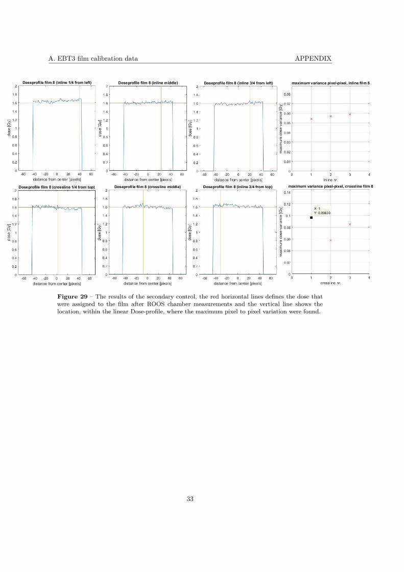
A. EBT3 film calibration data APPENDIX

Figure 29 – The results of the secondary control, the red horizontal lines defines the dose thatwere assigned to the film after ROOS chamber measurements and the vertical line shows thelocation, within the linear Dose-profile, where the maximum pixel to pixel variation were found.

33

APPENDIX B. Range effects including bone equivalent plates, additional images and data

B Range effects including bone equivalent plates, addi-tional images and data

Due to the fact that multiple implants were tested in this setup the data will be presented for eachimplant separately but all simulations were compared to the reference simulation seen in Fig. 30. Thetabulated values were the ones used to create the curves in Fig. 18.

Figure 30 – The reference Eclipse simulation for the range shift tests to which the bone plateswere included.

34

B. Range effects including bone equivalent plates, additional images and data APPENDIX

B.1 implant 1In Fig. 31 and 32 the two Eclipse simulations (both the original and the iMAR enhanced) used in thetest can be seen.

Figure 31 – The Eclipse simulation usedin the range effect test for implant 1 forthe setup that included the bone equiva-lent plates.

Figure 32 – Basically the same simula-tion but here performed on a CT-imagebase that had been improved using theiMAR software.

Figure 33 – The depth profiles from which the simulated shift in R50 for implant 1, with thesetup that included the bone equivalent plates, were calculated.

35

APPENDIX B. Range effects including bone equivalent plates, additional images and data




Figure 36 – The depth profiles from which the simulated shift in R50 for implant 2, with thesetup that included the bone equivalent plates, were calculated.

36

B. Range effects including bone equivalent plates, additional images and data APPENDIX




37

APPENDIX C. Range effects excluding bone equivalent plates, additional images and data

C Range effects excluding bone equivalent plates, addi-tional images and data

Due to the fact that multiple implants were tested in this setup the data will be presented for eachimplant separately but all simulations were compared to the reference simulation seen in Fig. 39. Thetabulated values were the ones used to create the curves in Fig. 20.

Figure 39 – The reference Eclipse simulation for the range shift tests to which the bone plateswere excluded.

38

C. Range effects excluding bone equivalent plates, additional images and data APPENDIX

C.1 implant 1

In Fig. 40 and 41 the two Eclipse simulations (both the original and the iMAR enhanced) used in thetest can be seen.

Figure 40 – The Eclipse simulation usedin the range effect test for implant 1 forthe setup that excluded the bone equiva-lent plates.

Figure 41 – Basically the same simula-tion but here performed on a CT-imagethat had been improved using the iMARsoftware.

C.2 implant 2

In Fig. 42 and 43 the two Eclipse simulations (both the original and the iMAR enhanced) used in thetest can be seen.



39

APPENDIX C. Range effects excluding bone equivalent plates, additional images and data

Figure 44 – The depth profiles from which the simulated shift in R50 for implant 2, from thesetup that excluded the bone equivalent plates, were calculated.

40

D. Lateral dose distribution, additional images and data APPENDIX

D Lateral dose distribution, additional images and data

As there is a multitude of implants that are studied in this test the data will be presented implant forimplant. In the following subsections within this appendix data for measurements on several depths willbe presented, these depths are defined as the positions described in Tab. 4 most of the measurementswere performed with the positions within the ”deep” part of the table and the ones marked ”surface”performed with the positions in the part named so.

D.1 The reference (deep setup)

Figure 45 – The eclipse simulation of the reference setup for the lateral dose distribution study.

In Fig. 45 the Eclipse simulation of the reference setup for the lateral dose distribution measurements,the following sections contains comparisons between the implant measurements and this reference.

41

APPENDIX D. Lateral dose distribution, additional images and data

D.2 Implant 1 (deep setup)

Figure 46 – Comparisons of the linear lateral dose profiles in crossline direction for the film measure-ments of implant 1, film measurements with the reference setup and the corresponding Eclipse simulationprofiles at position (deep) 1-8.

Figure 47 – Comparisons of the linear lateral dose profiles in inline direction for the film measurementsof implant 1, film measurements with the reference setup and the corresponding Eclipse simulationprofiles at position (deep) 1-8.

42



Figure 48 – Comparisons of the linear lateral dose profiles in crossline direction for the film measure-ments of implant 2, film measurements with the reference setup and the corresponding Eclipse simulationprofiles at position (deep) 1-8 .


43





44





45





46





47


D.8 The reference, surface target

Figure 58 – The eclipse simulation of the reference setup for the lateral dose distribution studywith the surface setup.

In Fig. 58 the Eclipse simulation of the reference setup for the lateral dose distribution measurementswith the surface target is displayed. This plan is what has been used within the comparisions

D.9 Implant 1 (surface setup)

Figure 59 – Comparisons of the linear lateral dose profiles in crossline direction for the film measure-ments of implant 1, film measurements with the reference setup and the corresponding Eclipse simulationprofiles at position (surface) 1-8 .

48


Figure 60 – Comparisons of the linear lateral dose profiles in inline direction for the film measurementsof implant 1, film measurements with the reference setup and the corresponding Eclipse simulationprofiles at position (surface) 1-8.

D.10 Implant 2 (surface setup)

Figure 61 – Comparisons of the linear lateral dose profiles in crossline direction for the film measure-ments of implant 2, film measurements with the reference setup and the corresponding Eclipse simulationprofiles at position (surface) 1-8 .

49


Figure 62 – Comparisons of the linear lateral dose profiles in inline direction for the film measurementsof implant 2, film measurements with the reference setup and the corresponding Eclipse simulationprofiles at position (surface) 1-8.

50

masterthesisreport -...

Documents