Master Thesison

Classification of Percussive Sounds usingMachine Learning

Nicolai GajhedeSound and Music Computing

AAU-CPH

Spring2016

Acknowledgements

A special thanks to my supervisor Assistant Professor Dr. Hendrik Purwins, from Faculty ofEngineering and Science, Aalborg University Copenhagen and AI and Machine Learning expertOliver Beck. Their valuable advice and guidance during my thesis have been much appreciated.

And my family for their support and understanding my absence.

Abstract

In this master thesis the focus have been on machine learning using convolutional neural networksand more specifically multi-class classification of percussive instruments. Recent advances in theCNN domain makes this a competitive field of research compared with other machine learningalgorithms. I present a modified CNN based on work from different past and present research.Different architectures of networks have been tested in this work. The fundamental networkof the new networks I have contributed with has shown promising results on its own. It alsoperforms well, regardless of the techniques applied internally (i.e. batch normalization, 50 %dropout). The results are gathered from a dataset comprising 3713 sound files consisting of bothdigital and acoustic recordings, through multiple epoch experiments and preliminary testing.

Contents

I Machine Learning 1

1 Introduction 21.1 State of The Art . . . . . . . . . . . . . . . . . . . . . . . . . . . . . . . . . . 3

1.1.1 Google - The Inception Network . . . . . . . . . . . . . . . . . . . . . 31.1.2 Microsoft - Deep Residual Learning . . . . . . . . . . . . . . . . . . . 41.1.3 Mxnet - GitHub Repository . . . . . . . . . . . . . . . . . . . . . . . 5

1.2 Related Work - Different Approach . . . . . . . . . . . . . . . . . . . . . . . . 61.2.1 Environmental Sound Classification . . . . . . . . . . . . . . . . . . . 61.2.2 Automatic Instrument Recognition . . . . . . . . . . . . . . . . . . . . 71.2.3 Musical Instrument Classification . . . . . . . . . . . . . . . . . . . . 71.2.4 Nonnegative Matrix Factorization . . . . . . . . . . . . . . . . . . . . 9

1.3 Final Problem Statement . . . . . . . . . . . . . . . . . . . . . . . . . . . . . 10

2 Analysis 112.1 The Digital Neural Network for Machine Learning . . . . . . . . . . . . . . . 11

2.1.1 Bagging . . . . . . . . . . . . . . . . . . . . . . . . . . . . . . . . . . 122.1.2 Dropout . . . . . . . . . . . . . . . . . . . . . . . . . . . . . . . . . . 122.1.3 Regularization . . . . . . . . . . . . . . . . . . . . . . . . . . . . . . 122.1.4 Backpropagation . . . . . . . . . . . . . . . . . . . . . . . . . . . . . 132.1.5 Gradient Descent . . . . . . . . . . . . . . . . . . . . . . . . . . . . . 13

2.2 Activation Functions . . . . . . . . . . . . . . . . . . . . . . . . . . . . . . . 142.2.1 Hyperbolic Tangent . . . . . . . . . . . . . . . . . . . . . . . . . . . . 142.2.2 Rectified Linear Function . . . . . . . . . . . . . . . . . . . . . . . . 142.2.3 Logistic Function . . . . . . . . . . . . . . . . . . . . . . . . . . . . . 15

2.3 Research in Convolutional Neural Networks for Sound and Music . . . . . . . 162.4 Musical Onset Detection . . . . . . . . . . . . . . . . . . . . . . . . . . . . . 16

2.4.1 Improved Musical Onset Detection . . . . . . . . . . . . . . . . . . . 172.5 Batch Normalization in Convolutional Neural Networks . . . . . . . . . . . . . 182.6 Music Boundary Detection . . . . . . . . . . . . . . . . . . . . . . . . . . . . 19

2.6.1 Music Structure Analysis . . . . . . . . . . . . . . . . . . . . . . . . . 192.6.2 Self-similarity Matrices . . . . . . . . . . . . . . . . . . . . . . . . . 202.6.3 Combined Features and Two-level Annotations . . . . . . . . . . . . . 21

2.7 Requirements Specification . . . . . . . . . . . . . . . . . . . . . . . . . . . . 22

i

II The Learning Algorithm 23

3 Design 243.1 The Prerequisites for the Network . . . . . . . . . . . . . . . . . . . . . . . . 24

3.1.1 Application Design . . . . . . . . . . . . . . . . . . . . . . . . . . . . 25

4 Implementation 284.1 Data Preparation . . . . . . . . . . . . . . . . . . . . . . . . . . . . . . . . . 28

4.1.1 MATLAB . . . . . . . . . . . . . . . . . . . . . . . . . . . . . . . . . 284.1.2 Quantile Based Representation . . . . . . . . . . . . . . . . . . . . . . 314.1.3 Im2rec Tool . . . . . . . . . . . . . . . . . . . . . . . . . . . . . . . . 334.1.4 Python Scripting . . . . . . . . . . . . . . . . . . . . . . . . . . . . . 33

4.2 The Network Architecture . . . . . . . . . . . . . . . . . . . . . . . . . . . . 354.2.1 Fundamental CNN Variant . . . . . . . . . . . . . . . . . . . . . . . . 354.2.2 Network Variants . . . . . . . . . . . . . . . . . . . . . . . . . . . . . 36

III Evaluation 37

5 Testing 385.1 Initial Testing . . . . . . . . . . . . . . . . . . . . . . . . . . . . . . . . . . . 38

5.1.1 Initial experiment quantile MLS vs normalized MLS . . . . . . . . . . 385.2 CNN Testing . . . . . . . . . . . . . . . . . . . . . . . . . . . . . . . . . . . 39

5.2.1 Testing Different Learning Rate on CNN with N-MLS . . . . . . . . . 405.2.2 Testing Different Learning Rates on CNN with N-MLS implementing

ReLU and Sigmoid . . . . . . . . . . . . . . . . . . . . . . . . . . . . 405.2.3 Fundamental CNN with Batch Normalization and Dropout on Normal-

ized MLS . . . . . . . . . . . . . . . . . . . . . . . . . . . . . . . . . 41

6 Evaluating the Results 426.1 Test Evaluation . . . . . . . . . . . . . . . . . . . . . . . . . . . . . . . . . . 42

6.1.1 Fundamental Network . . . . . . . . . . . . . . . . . . . . . . . . . . 436.1.2 Dropout Network . . . . . . . . . . . . . . . . . . . . . . . . . . . . . 436.1.3 Batch Normalization Network . . . . . . . . . . . . . . . . . . . . . . 446.1.4 Combined Dropout and Batch Normalization . . . . . . . . . . . . . . 44

6.2 Subconclusion . . . . . . . . . . . . . . . . . . . . . . . . . . . . . . . . . . . 45

IV Finalization 46

7 Discussion 477.1 Network Parameters . . . . . . . . . . . . . . . . . . . . . . . . . . . . . . . . 48

7.1.1 Learning Rate . . . . . . . . . . . . . . . . . . . . . . . . . . . . . . . 487.1.2 Activation Functions . . . . . . . . . . . . . . . . . . . . . . . . . . . 487.1.3 Batch Size . . . . . . . . . . . . . . . . . . . . . . . . . . . . . . . . 48

ii AAU-CPH

7.1.4 Number of Filters . . . . . . . . . . . . . . . . . . . . . . . . . . . . . 487.1.5 Depth of Network . . . . . . . . . . . . . . . . . . . . . . . . . . . . 497.1.6 Filter Kernels . . . . . . . . . . . . . . . . . . . . . . . . . . . . . . . 49

7.2 Network Variants . . . . . . . . . . . . . . . . . . . . . . . . . . . . . . . . . 497.2.1 Dropout . . . . . . . . . . . . . . . . . . . . . . . . . . . . . . . . . . 497.2.2 Batch Normalization . . . . . . . . . . . . . . . . . . . . . . . . . . . 507.2.3 Observations . . . . . . . . . . . . . . . . . . . . . . . . . . . . . . . 50

8 Conclusion 51

V Appendix 56

A The Prediction Script 57

B The Network Script with Fundamental Structure 59

C The Network Script with Dropout 62

D The Network Script with Batch Normalization in All Convolutional Layers 65

E The Network Script Combining Dropout and Batch Normalization 69

F Audio Input Preprocessing 72

G Low-level Parameters 76

H Lst File for Iterator 80

I JSON File Created From Training 81

iii AAU-CPH

List of Figures

1.1 Illustration showing the "Inception"-module used in the CNN by GoogLeNet [6]. 31.2 Illustration showing the development of error rates using plain and residual

networks on the ImageNet dataset [7]. . . . . . . . . . . . . . . . . . . . . . . 51.3 Illustration showing the preprocessing methodology from the fusion approach [4]. 81.4 Illustration showing the CNN using two different input representation of the

audio signal [4]. . . . . . . . . . . . . . . . . . . . . . . . . . . . . . . . . . . 81.5 Illustration showing the approximation of the input from two atoms and their

activations [19]. . . . . . . . . . . . . . . . . . . . . . . . . . . . . . . . . . . 10

2.1 Illustration showing the network architecture used for onset detection [3]. . . . 162.2 Illustration showing the results from different experimental setups for onset

detection [3]. . . . . . . . . . . . . . . . . . . . . . . . . . . . . . . . . . . . 182.3 Illustration showing the four different architecture for fusion of combined features.

[16]. . . . . . . . . . . . . . . . . . . . . . . . . . . . . . . . . . . . . . . . . 202.4 Illustration showing the network architecture for the different input strategies and

output. [17]. . . . . . . . . . . . . . . . . . . . . . . . . . . . . . . . . . . . . 21

3.1 Illustration showing different sound waves from the different drums in MATLAB. 253.2 Illustration of the flow from database to application output and usage. . . . . . 26

4.1 Illustration showing different training examples created in MATLAB from left toright: A), B), C) and D). . . . . . . . . . . . . . . . . . . . . . . . . . . . . . 32

4.2 Illustration showing the final representation of different sounds in the shape 80x8created in MATLAB. . . . . . . . . . . . . . . . . . . . . . . . . . . . . . . . 33

4.3 Illustration showing the fundamental CNN architecture created in the Python script. 35

iv

List of Tables

5.1 Table showing epoch number and accuracies in percentage of training and valida-tion data using tanh. . . . . . . . . . . . . . . . . . . . . . . . . . . . . . . . . 39

5.2 Table showing epoch number and accuracies in percentage of training and valida-tion data using ReLU and sigmoid functions. . . . . . . . . . . . . . . . . . . 39

5.3 Table showing dataset divided into training and validation data. . . . . . . . . . 405.4 Table showing epoch number and accuracies in percentage of training and valida-

tion data. . . . . . . . . . . . . . . . . . . . . . . . . . . . . . . . . . . . . . 405.5 Table showing epoch number and accuracies in percentage of training and valida-

tion data. . . . . . . . . . . . . . . . . . . . . . . . . . . . . . . . . . . . . . 415.6 Table showing epoch number and accuracies in percentage of training and valida-

tion data . . . . . . . . . . . . . . . . . . . . . . . . . . . . . . . . . . . . . . 41

v

Part I

Machine Learning

1

Chapter 1

Introduction

In recent years the popularity of convolutional neural networks (CNN) have regained strength inmany areas of machine learning, perhaps mostly within image processing and object recognition.Needless to say, it is a well known method used in computer vision problems and also nowprospering within sound and music. The fundamental techniques can be dated back to theseventies and the late eighties, where Lecun et. al. made groundbreaking progress for the postalsystem in the United States of America. The team used CNN with backpropagation to developautomatic and digital processing of handwritten zip codes on mails sent through Buffalo postalservices [1]. The network structure by Lecun et. al. have been widely used as starting point bydifferent authors during MNIST, Cifar-10 and ImageNet classification challenges [13, 12, 6].

The purpose of my thesis project is to use CNN for classification of percussive sounds inmusic, initially based on networks used in other research project and use these as starting pointfor development of a new network architecture. Furthermore I will adapt my network to newmethods and investigate how this influence the performance.

Non-linear classification problems are solvable using supervised learning using logisticregression, using many polynomial terms for the features. When the specific classificationproblem involves more than two features that are non-linear, it becomes impossible to includemore features in a 2 dimensional space [26].

There are different approaches that can be used with neural networks. The choices can varybetween creating a network from scratch together with training the model. Another option isto use a existing network architecture and train weights of the network based on a new dataset.Finally transfer learning can be used to extend an existing network and the dataset that it iscreated for. For more information about this approach I refer to [23]. The final option has severaldrawbacks in relation to this project, referring to the models I will describe in my thesis and willnot make sense semantically, when using sound representations as data input.

Several works have aimed to improve the neural networks, using one data source or multiplesources [4].

I will not go into details about the human auditory system in this thesis and the basics ofFourier transform etc. I assume that readers of this work to this extent are familiar with thefundamentals of sound and music from a human perspective and mathematical.

2

1.1 State of The Art

Multiple times each year in recent time, the barrier for state of the art has advanced due to newrequirements for research, implementation and experiments involving neural networks. Theresults from training networks with deeper and deeper networks with various modifications haveshown to be promising and better than the previous. In this section I will give examples ofresearch made recently that has contributed to this rapid positive development.

1.1.1 Google - The Inception Network

A group from Google Inc. who have named themselves GoogLeNet have been competing atthe ILSVRC 20141 with their network architecture they call "Inception", a 22-layer model. Thenetwork is described in a paper published in 2014. In this particular paper, the authors explainhow the network have been developed and under which requirements. The most relevant formy thesis project are the network architecture and the results from using this network on largerdatasets. On that note, I will not describe the requirements presented to the GoogLeNet groupwhen participating in the ILSVRC challenges [6]. The authors argue, the most straightforwardway to enhance a neural network in to increase both depth and width. Meaning that both the layeramount is increased and also the units within each layer. The cons of this approach is the severalparameters additional following changing the size to bigger and bigger. Consequently the trainingprocess is more exposed to the concept of overfitting. Besides danger of slowing or even stoppingtraining using the network because of what the authors call bottleneck, the computational cost arealso increased when the network is widened [6].

Figure 1.1: Illustration showing the "Inception"-module used in the CNN by GoogLeNet [6].

The chosen idea for the "Inception" network is based on using modules with 1x1 convolutionalunits to reduce dimensions of a given layer, preferably the layers that would otherwise beexpensive computationally since they contain 3x3 and 5x5 convolutional units. See the figureabove 1.1 for a full example of an "Inception"-module. These 1x1 units also contains rectifiedlinear activation functions. Only on higher layers are these modules with 1x1 units applied and inthe starting layers, the traditional convolutional is maintained [6]. For the full network design Irefer to [6].

1ImageNet Large Scale Visual Recogtion Challenge - http://www.image-net.org/challenges/LSVRC/

3 AAU-CPH

The results from using these "Inception"-modules were enough for the GoogLeNet to winthe challenge they participated in by a error rate of 6,67 %. That is calculated as an 56,5 %improvement from the 2012 contenders first place [6].

Rethinking the Inception Network Architecture

New ideas, algorithms and results have been presented by Google Inc. since the first "Incep-tion" network described above 1.1.1. In a recent paper from 2015 the Szegedy et. al. haveexplored modifications to improve previous work and performance of winning model. Theauthors mentions that the existing model can be difficult adapting it to other problems and stillpreserve the efficiency. As an example, if the filter banks are doubled throughout the network, thecomputational costs and parameters following with increase times 4 [11].

The four new ideas and design principles the authors suggest to improve the "Inception"network with are as follows:

1. The representation sizes should decrease in a smooth way from input to output.2. Increasing units in hidden layers of the network.3. Reducing the input representation before performing spread out convolutions (e.g. 3x3 or 5x5).4. Increasing the width and depth of the network should increase performance of the network [11].

An interesting point found by doing control experiments in the research are that asymmetricconvolutions can decrease the computational cost (i.e. 33 %), if the square convolution areseparated in two layers. While decreasing the size of a convolutional kernel from 3x3 to 2x2 onlysaves less on the costs (i.e. 11 %). The constraint from this experiment is that the new idea doesnot apply well to starting layers. The technique should be used in layers where feature maps of mx m and m ranges from 12-20 [11].

The new network size have increased to a 42-layer deep network and several layers havebeen changed from large 7x7 filter to sequential 3x3 filters. The computational cost have alsoincreased approximately 2,5 times than the previous "Inception" network. The authors elaborateson the common consensus that high resolution of the input to the first layers of a network lead tobetter recognition performance. The drawback from this fact shows; the network computationalcost rise [11]. The authors found no significant evidence for removing the first pooling layer oftheir network and it would decrease computational costs [11].

1.1.2 Microsoft - Deep Residual Learning

In the same domain of research and approximately same time of the year as the previous paper, apaper from Microsoft Research has been published on deep neural networks for image processing.The authors behind this project have been looking into questions such as, if neural networksimproves by using more layers between input and output. They have presented a network of34-layers and compares it to an identical one of 18-layers, furthermore with simple plain networksof same sizes [7].

4 AAU-CPH

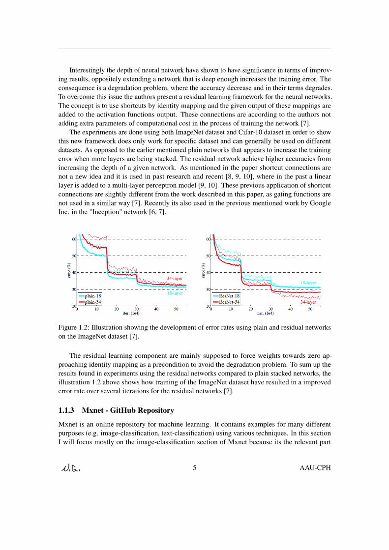
Interestingly the depth of neural network have shown to have significance in terms of improv-ing results, oppositely extending a network that is deep enough increases the training error. Theconsequence is a degradation problem, where the accuracy decrease and in their terms degrades.To overcome this issue the authors present a residual learning framework for the neural networks.The concept is to use shortcuts by identity mapping and the given output of these mappings areadded to the activation functions output. These connections are according to the authors notadding extra parameters of computational cost in the process of training the network [7].

The experiments are done using both ImageNet dataset and Cifar-10 dataset in order to showthis new framework does only work for specific dataset and can generally be used on differentdatasets. As opposed to the earlier mentioned plain networks that appears to increase the trainingerror when more layers are being stacked. The residual network achieve higher accuracies fromincreasing the depth of a given network. As mentioned in the paper shortcut connections arenot a new idea and it is used in past research and recent [8, 9, 10], where in the past a linearlayer is added to a multi-layer perceptron model [9, 10]. These previous application of shortcutconnections are slightly different from the work described in this paper, as gating functions arenot used in a similar way [7]. Recently its also used in the previous mentioned work by GoogleInc. in the "Inception" network [6, 7].

Figure 1.2: Illustration showing the development of error rates using plain and residual networkson the ImageNet dataset [7].

The residual learning component are mainly supposed to force weights towards zero ap-proaching identity mapping as a precondition to avoid the degradation problem. To sum up theresults found in experiments using the residual networks compared to plain stacked networks, theillustration 1.2 above shows how training of the ImageNet dataset have resulted in a improvederror rate over several iterations for the residual networks [7].

1.1.3 Mxnet - GitHub Repository

Mxnet is an online repository for machine learning. It contains examples for many differentpurposes (e.g. image-classification, text-classification) using various techniques. In this sectionI will focus mostly on the image-classification section of Mxnet because its the relevant part

5 AAU-CPH

for this report and my thesis work. The options in Mxnet are many in terms of programminglanguage and network examples. I focus on CNN for this semester and Mxnet has provided lotsof examples for exactly this area.

The primary language I have used is Python and I have explored the folder “image-classification”to a large degree. I have been going through many of the network example files and seen howtheir implementation is structured in the scripts. Some scripts are dependent on other files suchas “symbol” files for training. In the older network, the network is started directly from e.g.train_mnist.py, while more recent and large network are trained from “train_imagenet.py” andthen the “symbol” file containing the network architecture is passed as an argument to the scriptcall.

All the created models are utilizing the script: “train_model.py” to account for momentumof the algorithm and the accuracy output [25].

1.2 Related Work - Different Approach

In this section I will describe research that is closely related to my thesis work, using differenttechniques and still within the domain of neural networks for sound and music applications. Thesection will cover work from environmental sounds, speech recognition and musical instrumentclassification.

1.2.1 Environmental Sound Classification

Research in environmental sounds contain a wide spectra of different sounds and they can beproduced by very different elements in nature and our everyday surroundings. The article I want tofocus on first in this section is from 2015 and uses 3 publicly available datasets of environmentaland urban recordings.

The network used by the author is not particularly deep or spectacular in width. It does howeverhave some interesting properties as it utilize segmented spectrograms with deltas as 2-channelinput to the network.

The training examples in the environmental sound dataset was separated into short andlong representations, then converted in to log-scaled Mel-spectrograms2. These examples wereresampled to 22050 Hz and normalized. The windows size used for the creating the spectrogramswas 1024 samples and a hop size of 512 samples. The result was a 60-band Mel-frequency bands.A general rule for these short and long representations was 41 frames with 50 % overlap for theshort versions and 101 frames with 90 % overlap for the long. The representations was providedwith delta, calculated from a external library and was functional as input for the network.

The network is similar to the one presented by [1] and contains two convolutional layerswith rectified linear activations each followed by max-pooling layer. Finally two fully-connectedlayers with 5000 filters each and a Softmax classifier for the output. During training the shortexamples was stopped after 300 epochs and the long after 150 epochs using learnings rates of0.002 and 0.01 respectively.

2Mel refers to the Mel-scale of linearly spaced frequencies for low frequencies and logarithmically for high

6 AAU-CPH

The results presented from this study are not extensive and the authors argue only, that usingCNN achieves a similar level of performance as other methods [14].

1.2.2 Automatic Instrument Recognition

One of two related papers I will go into concerning instrument recognizing were published in2015 by Li et al. with the focus on using raw audio data for training a CNN [20].

They create a network with 3 convolutional layers with max-pooling and rectified linearactivations. Furthermore they have two fully-connected layers, with rectified activations in thefirst fully-connected, as in the convolutional layer and dropout for that particular fully-connectedlayer. In the second fully-connected layer they use sigmoid for the output units. In their methodthe authors compared the predicted activations with training activations using a binary crossentropy loss function [20].

Using a batch size of 16 and stochastic gradient descent the author train the CNN afterpreprocessing the input data. Setting the labels for the 11 groups of instruments they decidedto use were not a trivial approach, since their annotations covered 82 instruments. The authorscontinued by grouping these into 70 classes, afterwards they collected all groups appearing inless than 20 songs into a class called "others" [20].

After categorizing the instruments the authors calculated normal MFCCs but also first andsecond order differences, ending with three matrices for benchmarks. The matrices were modeledby a Gaussian distribution [20].

Finally the authors compared they CNN with the calculated benchmarks and found the CNNto outperform other methods [20].

1.2.3 Musical Instrument Classification

Instruments are an essential part of music and sounds for musical performances. I want to presentthe next study due to its relevance for my thesis and the technical setup of it. The investigatedapproach using CNN for instrument classification was published in 2015.

The main idea is to combine spectrograms as input to a CNN with multi-resolution recurrenceplots (MRP). The MRP representation contain phase information about the audio signal in a twodimensional layout. The phase attribute can be very useful when distinguishing between differentinstruments. The authors use 8 different length spectrograms excerpts for one input and 56 (7layers x 8 points) MRP images of different temporal block size and resolution of the MRP for theother input [4]. See figure 1.3.

7 AAU-CPH

Figure 1.3: Illustration showing the preprocessing methodology from the fusion approach [4].

Before creating the MRP representations the authors use 1 dimensional max-pooling ofthe signal, they preserve temporal changes of the origin of the raw audio signal while stillimproving the classification performance. After generation of the MRP from this reduced signal,they also reduce the size of the image by using another max-pooling step to the 2 dimensionalrepresentation of MRP, resulting in a smaller image size. In the preprocessing step of the project,the authors does not normalize the magnitude of the MRP image because of the relation to attackand transient shape of the audio signal this conveys [4].

Three different combinations of double input to the CNN was used in this study. One thatuses only the MRP, the second for only spectrograms and the third is both MRP and spectrograms.The network architecture is composed of two convolutional layers with max-pooling and rectifiedlinear activations, a layers for merging the output from the previous layers before a fourth layerof fully-connected units and Softmax classifier for the output. The network can be seen in figure1.4 [4].

Figure 1.4: Illustration showing the CNN using two different input representation of the audiosignal [4].

8 AAU-CPH

The 3 objectives the authors proposed was; classifying 4 instrument families from 20 instru-ments, classifying each instrument and lastly using their own dataset classifying 4 different pianosusing a single note. From the 3 different tasks using the 3 different combinations of network, theauthors noted a classification error of 1.31 %, 6.35 % and 6.86 % for the three tasks, using thecombined network of spectrogram and MRP respectively. The combined network performed bestin all three tasks. While the spectrogram approach performed better than the MRP version in thetwo first tasks, but not in task three [4].

1.2.4 Nonnegative Matrix Factorization

As the final part in this introductory chapter, before starting the next, I want to make a final noteon different approaches to sound and music processing. Formally the concept of nonnegativematrix factorization (NMF) is presented as a compositional model for audio processing. Mathe-matical models that are represented as nonnegative linear combinations used to explain data (i.e.sound and music). The concept is primarily used in audio processing to approximate a low-levelparametric representations such as the spectrograms using matrices and reconstructing the sounds.

NMF models are nonnegative time-frequency representations of a given signal as matrices.They are decomposed into products of component matrices that are nonnegative. One matrixrepresent the atomic parts, pattern wise, and the another matrix represent the activations to thesignal over time. The job of the NMF is to estimate the atoms and their activations from a mixtureof sounds in a signal (e.g. music pieces). Furthermore the NMF can utilize atoms to combinea model from training data linearly [19]. In order to represent the signal as matrices, the signalmust be decomposed and to do so one can find a divergence using a mathematical approach. Theobserved spectrograms of the signal must be approximated by two matrices and the divergencecan be used to control for most optimal approximation. The commonly used divergence functionin matrix decomposition is the squared error. When being in the NMF framework regularizationterms can be used to constrain the divergence and minimize it. I will go further into regularizationas part of the classification task with neural networks in the next chapter [19]. Figure 1.5 showsthe decomposition concept of NMF.

A limitation to the NMF model can be seen if a spectrogram, due to technical preprocessingissues, are not represented to its full extend and are missing frames. The NMF cannot be usedand ignore (or reconstruct) the missing frame values, as there is simply no data to express theactivation for the atoms affected by the missing frames. Another limitation to compositionalmodels overall, coming back to the time-frequency representations of spectrograms often usedin this context; they lack phase information and consequently makes reliable sound synthesisdifficult [19].

As study have indicated NMF can be used for instrument classification as well using differentparameterized sound features e.g. zero crossings, spectral centroid, MFCCs. The highestperformance of a set NMF experiments was 95.5 % in classification accuracy. The authors used anearest-neighbor classifier for the weights of the vectors of the NMF output, applying a cosinesimilarity matrix to determine the right instrument [22].

9 AAU-CPH

Figure 1.5: Illustration showing the approximation of the input from two atoms and theiractivations [19].

I will not spend more time on experimenting or considering NMF methods as they are out ofscope for this project. The idea with mentioning it was as indicated by this section title, to presentrelated research with a different approach.

1.3 Final Problem Statement

As an extension to this introduction and a midway point before I start analyzing research andconcepts within the academic area of machine learning for sound and music computing. I wouldlike to present my final problem statement, which I will aim to answers throughout this report.

Can a CNN be used to classify percussive sounds and predict the correct label for a givenpercussive instrument? Will the classification accuracy be improved using some of the newesttechniques in the literature and by altering fundamental algorithm parameters? Will the CNNperform similarly or better than the existing networks does on instrument classification andrecognition?

10 AAU-CPH

Chapter 2

Analysis

The second chapter in this first part of this report will describe and also depicts several studiesmade within machine learning for musical applications. It will aim to clarify the most usedterminology in machine learning (i.e. neural networks used with sound and music), including theconcepts behind. In order to replicate essential network settings beneficial for my thesis, I willgo into more details with the selected relevant studies. Beginning with a general description ofneural networks.

2.1 The Digital Neural Network for Machine Learning

Neural Networks are a known and well documented techniques for machine learning [1, 13, 6, 3,7, 24]. In order to train a neural network several mathematical equations are being used for calcu-lation. Forward propagation for algorithm weights of filter and results according to the trainingsets’ features (x(i)). A cost function (Jθ ) using for instance a sigmoid curve and backpropagationto compute partial derivatives (α/αθ ) for deltas (δ ) to minimize the cost function.

The normal procedure for training a neural network consist of 6 general steps:

1. Randomly initialize weights.2. Implement forward propagation to get hθ (x(i)) for any x(i).3. Implement equation for the cost function.4. Implement backward propagation for computing partial derivatives.5. Use gradient checking for comparing partial derivatives computed using backpropagationversus numerical estimate of gradient of J(θ ).6. Use gradient descent or another advanced optimization algorithm with backpropagation tominimize the cost function J(θ ) as a function of parameters θ [26].

When trying to evaluate and improve the learning algorithm of the network some developerstry multiple approaches e.g. to get more training examples, try smaller set of features, try gettingadditional features, try to add polynomial features etc. In many situations these are redundantways of trying to better the results of outcomes given by the training set [26].

11

The steps shown above will indicate a thoroughly considered way of creating a neural net-work from scratch. The goal of my work will be improving methods for neural networks andsuggest new alternatives to how a network can be used in sound classification.

2.1.1 Bagging

Several working implementations of neural network use bagging as a mean of improving theclassifier [3]. A method based on averaging the output of CNN or RNN 1 and here achieving ahigher F-score or validation accuracy. Bagging has certain limitations and eventhough it improvesscores for 2 CNN, it does not increase F-score for 4 CNN. Learning two CNN separately will notgive either of the network the advantage, as they are trained individually, while bagging of thetwo networks can improve the collected performance in terms of score. A significant issue of thismethod is the increment of computational cost, two identical networks that are used will doublethe cost. [3, 15].

2.1.2 Dropout

As the neural networks often contain one or more layers of hidden units, dropout is a methodfor ensuring units to obtain learning from one another, while still solving independently of theprevious units in the network. During training using dropout the output of hidden layers arerandomly dropped according to a defined percentage of the units in the layers (e.g. 50 %). Thetechnique is often applied to avoid overfitting. The advantage of using dropout besides what wasjust mentioned is; not increasing computational cost as opposed to bagging which can double thecosts [14, 26, 3].

2.1.3 Regularization

In order to avoid overfitting the regularization technique can be used. The idea of applying thismathematical term to a hypothesis, is to keep the values of the parameters small when calculatingthe cost function. The equation below shows the regularization term for linear regression. With asmall value of lambda (λ ), not using much regularization, there is a higher risk of overfitting [26].

λ

2m

m

∑j=1

θ2j (2.1)

The case of overfitting can be caused by having too many features describing the trainingexamples in a dataset. The learned hypothesis may then fit the particular training data well butwill not generalize to new examples of training data when predicting labels. Following overfittingis often the concept of high variance and the curve used to fit the training data is often composedof several high-order polynomials features or too many [26].

1Recurrent Neural Network

12 AAU-CPH

2.1.4 Backpropagation

The learning algorithm called backpropagation is often used in the gradient descent computation.The partial derivative terms in the gradient descent can be calculated using this algorithm. Usuallythe output of the activation functions for each neuron in the network layers are calculated usingforward propagation. The calculation for the backpropagation starts in the output layer after theforward propagation is completed and uses delta terms for the derivatives to return at the firsthidden layer in the network layers by layer. The partial error delta terms are calculated as [26]:

δ (L) = a(L)− y(i) (2.2)

Hence the backpropagation calculates the error between the predicted output and the realoutput for the first delta term. Then moving back in network and adjusting the weights of thehidden layers by summation of weights times the delta terms for each layer [26].

2.1.5 Gradient Descent

In the traditional gradient descent (GD) the algorithm runs over the entire dataset and performs asummation of the whole, before updating parameters and moving closer to the local minimum ina somewhat straight line trajectory [26].

Stochastic Gradient Descent

The stochastic gradient descent (SGD) is often divided into 2 steps, where the first is to shuffle theentire dataset. The second is to look at a single training example and update the weights beforemoving to the next training example [26].

SGD is taking a small steps with respect to the cost function and modify the parametersslightly so it fits the cost function better. Then it goes to the next example and does the same.The downside of the SGD is that is not neccesarily converge at exactly the local minimum as thetraditional GD, though it in practice does not influence many algorithms as the weights values arechosen close to the local minimum [26].

The SGD is considered to be performing faster than traditional GD [26].

Mini-Batch Gradient Descent

A third version of the GD is called mini-batch gradient descent (MBGD) and works as the nameimplies on smaller batches than the entire batch of the whole dataset [26].

The normal range for MBGD is between 2-100 training examples from the total dataset. Thevalues of parameters are then updated after using these shuffled examples. The advantage ofusing MBGD compared to SGD is that the ability to parallelize increase if the computation of thealgorithms is vectorized in good way [26].

The MBGD is also considered to be faster than GD [26].

13 AAU-CPH

Feature Scaling

In order to achieve a faster convergence of the gradient descent, it is possible to scale the featuresin the dataset. Instead of having a large variation between minimum and maximum values withina feature, it can be beneficial to scale it to somewhere from 0-1 or -1 to 1. This can prompt thegradient descent to find a more direct path towards the global minimum. This procedure is mostlyadvantageous for problems with many different features that spans widely between minimum andmaximum values.

Learning Rate

Since the job of the gradient descent is to find the value of theta that minimizes the cost function.If the learning rate is set to high, there is danger of overfitting and not ending at the globalminimum as desired for the cost function. On the contrary of the learning is set very low, it willslow the progress of finding the minimum and results in a slow convergence problem for thegradient descent. Often the choice is a matter of trial by error, as the standards for automaticconvergence test are hard to determine thresholds for. Naturally it is hard to determine a threshold(e.g. a value in the range 10−3) for a decrease in the cost function, when a learning rate have notbeen chosen yet.

2.2 Activation Functions

In all implementations of neural networks a requirement for activation functions are presented toachieve convergence at the local minimum of the cost function. In this section I will describe thecommonly used. On a plot in a coordinate system, the functions can appear very similar but theirmathematical equations are different and I will show that here.

2.2.1 Hyperbolic Tangent

A non-linear function i.e. "tanh" can be used to obtain convergence fast, if the weights used arenot too small. If the weights are to small it will range from slow to very slow.

tanh(z) =e2z −1e2z +1

(2.3)

This can affect the amount of epoch necessary for the algorithm to converge at the optimalminimum.

2.2.2 Rectified Linear Function

A neuron or unit implementing a rectified linear function is called rectified linear unit (ReLU)and are found using the activation function:

f (x) = max(0,x) (2.4)

14 AAU-CPH

The advantage of using ReLU is that it addresses the saturation problem and consequently thevanishing gradient while training, which can slow down the convergence of a model being trained[5, 14].

2.2.3 Logistic Function

Sigmoid functions are often used in neural network layers because of its non-linearity.

y =1

1+ e−x (2.5)

The first derivative is computational efficient [21].

15 AAU-CPH

2.3 Research in Convolutional Neural Networks for Sound and Mu-sic

Going more into sound and music related to CNN. The following sections will further investigateresearch done focusing on sound and music for onset detection, and speech recognition with thegoal of identifying relevant information usable for this master thesis.

The proposed research have been selected in order to find relevant implementations ofconvolutional neural network (CNN) to classify and predict percussive sounds from dataset ineither image or human annotated format.

2.4 Musical Onset Detection

Jan Schlüter et al. have focused on finding onsets in polyphonic music using CNN.They have implemented a neural network that is similar to how image processing classify

different image classes by content, using spectrograms to detect annotated (ground-truth) onset inmusical recordings. It have been done within great success and motivated the authors to do morework in line of this article. I will elaborate on the differences between their work after describingtheir related articles.

Studying the first article it is shown how the authors improved the performance of theirclassification objective compared existing methods in the field for musical onset detection using aCNN. The figure 2.1 shows the architecture used for the network causing this improvement.

Figure 2.1: Illustration showing the network architecture used for onset detection [3].

The Data Input is based on:

• 3 spectrograms of 10 ms hop size, window size 23, 46 and 93.

• 80 band Mel frequency filter from 27,5 Hz to 16 kHz.

• Normalization of frequency bands to zero mean and unit variance.

16 AAU-CPH

• The input is in blocks of 15 frames.

• The learning rate is 0.05.

From this input the networks was evaluated using the procedure shown next.

The Evaluation is done according to:

• Training is done utilizing 100 epochs and 256 examples while the output is smoothed over timeand thresholded within a limit of +/- 25 ms of target annotation.

• Results are obtained from 8-fold cross validation.

The Network Implementation are resulting in:

The CNN performs better than RNN and reduce manual processing. The computational costs areincreased. Furthermore it is indicated from the results of this study that rectangular kernel filtershapes are outperforming conventional squared kernel filters.

In the given implementation max-pooling filters are wide in frequency and narrow in time andvice versa for convolutional filters. The final fully-connected layer is integrated from informationfrom previous fully-connected layer [2]

2.4.1 Improved Musical Onset Detection

The same authors as mentioned above have done extensive research based on the same networkarchitecture. In this section I will not describe the intention of the article as carefully, becauseit is alike their previous work. The same data input have been used here. The outcome of theirimplementation is providing different results, that are worth taking notice of and key elementsaccounting for these improved results can prove useful in future implementation of similarnetworks.

The Key Differences from the articles above are:

In this article the authors are randomly dropping 50 percent of the input units to the fully-connected layers and double the remaining weights. Also the annotated onsets are assigned to 3spectrograms instead of 1 as in 2.4 and weighting the extra frames less in training. Furthermorethe experiments conducted for the improved musical onset detection paper have looked at resultsfor different implementations of their network [3]. The figure 2.2 shows the results from theexperiments conducted in relation to onset detection.

17 AAU-CPH

Figure 2.2: Illustration showing the results from different experimental setups for onset detection[3].

Next I will go more into new techniques for implementations of CNNs.

2.5 Batch Normalization in Convolutional Neural Networks

Additional research in the field of machine learning with deep neural network has been proposedby the authors Sergey Ioffe and Christian Szegedy, their starting point is in the "Inception"network by Google Inc. described in section 1.1. They have initially worked with a method usingmini-batches of examples during training with stochastic gradient decent instead of using onlyone a example at the time. In the research they have made they claim several improvements byusing mini-batches, i.e. degree of loss over the mini-batch can be an estimate of the loss overan entire dataset. The estimate can be improved when increasing the batch size. Secondly theyargue that the computational efficiency is increased when using batches in parallel rather than onindividual examples of the full dataset [5].

The proposed concept of batch normalization is considered to improve training speed, byreducing the internal covariate shift in deep neural networks. The authors define the internalcovariate shift as a bi-product of change in network parameters during training. Network trainingconverges faster by transforming the input to zero mean and unit variance, leading to the idea oftransforming all input from previous layer in this way. And by doing so, reducing the internalcovariate shift happening before beginning the next layers in deep network [5].

The batch normalization transform is preferable applied before the nonlinearity by normaliz-ing x = Wu + b (the activation function) of each layers. The authors suggest to do the transformof the input for each layers, after the first input layer, as these are likely to be the sum of othernonlinearity and the distributed shapes changes during training. Their initial experiments haveshown that this does not reduce the covariate shift. Following the same procedure for bothfully-connected and convolutional layers, it can be achieved to have the normalization follow theconvolutional characteristics so that each kernel elements in different locations of feature map areidentically normalized throughout training [5].

Finally the authors suggests the advantage of using batch normalization is evident, whenlearning rates are high so that the gradient descent occasionally appears to be stopping at less

18 AAU-CPH

optimal local minimum while converging. This additionally leads to a conclusion that withbatch normalization the backpropagation in each layers in not influenced by the scale of layersparameters (e.g. high learning rate). For earlier techniques scaling of parameters may have causeda model to increase drastically in size or computational cost/time [5].

As a last remark to this research, it has also been found useful to utilize the above techniquesto limit the use of dropout, which have earlier been widely known for addressing overfitting [5].

2.6 Music Boundary Detection

I want to round this part and chapter off by discussing research done in related to boundarydetection using CNN. Thomas Grill et al. have investigated several different methods as solutionto this problem. It entails spectrograms with self-similarity lag matrices (SSLM), structureanalysis, combined features and two-level annotations.

2.6.1 Music Structure Analysis

In this first subsection I will focus on research done on music structure analysis (MSA) as the ’tipof the iceberg’, indicating that a large chuck of information is related to structure of music ormusical form. The work done is based on CNN and are close related to the work mentioned in2.4, the groups of authors both train a binary classifier on spectrograms from music segments.

The method described here is based on feature extraction and more precisely Mel-spectrograms.Additionally the author have used also MFCC, chroma vectors and fluctuation patterns, con-cluding that the modified spectrograms were making the network perform better than the otherfeatures mentioned. The three areas of interest to the final performance of the network aredifferent context length, temporal smearing and spectrogram resolution [15]. The spectrogramswas calculated over a window of 2048 samples at 44100 kHz, applying a Mel-filterbank of 80coefficients and triangular filter from 80 Hz to 16 kHz. The magnitudes of audio input was scaledlogarithmically and was padded with pink noise at -70 dB as the authors found useful [15].

The network architecture for this work was consisting of a convolutional layers of 16 kernelsof size 8 x 6. Then using a max-pooling layer of 3 x 6. Another convolutional layer of 32 kernelsof 6 x 3 and a fully-connected layer with 128 units. Finally they use one last fully-connectedlayer with one output unit. The authors mentioned that early experiments have determined thefundament for this network architecture [15].

The training was conducted using gradient descent of mini-batches with 64 training examples.The momentum was set to 0.95 and the learning rate starting at 0.6 and increased after everyepoch by multiplying with 0.85. The training procedure was stopped after 20 epochs in everyscenario [15].

The results of performance for this network have showed the authors were able to achieveF-score measures that perform better than previous attempts on the MIREX 2 dataset based onthe SALAMI 3 database they have used for human annotated data. One drawback of using thesound files from the database they have chosen, is the different loudness of the sounds, and they

2Music community campaign called: Music Information Retrieval Evaluation eXchange3A public available database named: Structural Analysis of Large Amounts of Music Information

19 AAU-CPH

suggest to use a more time of preprocessing in order to account for this issue before training thenetwork [15].

2.6.2 Self-similarity Matrices

As the second approach I will present a CNN based on spectrograms and SSLM. The main idea isto determine the transition points between the structural elements in a music pieces (e.g. phrases,chorus, verse).

In the literature Thomas Grill et al. describe their problem arise from the fact that Mel-spectrograms does not contain all the information about the audio data as they find fitting for thenetwork [16]. The SSM method can compare similarities from earlier checkpoints in time withina certain lag time. They can use this with low-level features and matrix representations of thesemetrics [16].

When extraction features the authors use a window of 2048 samples at 44100 kHz. And arevery similar to the extraction methods presented in the section above. A Mel-filterbank of 80triangular filter etc. From preliminary experiments the authors found MFCC and cosine distanceto yield better results than Euclidian metrics [16].

The CNN presented in the paper is built using four different architectures based on where tocombine the two input features (i.e. Mel-spectrograms, SSLM). Each ending in its own specificway to the output unit(s) in the network. As seen in the figure 2.3 below, architecture (a) isbased on an average of the two output units, (b) is joining the two output layers, (c) two hiddendense layers for the fusion and (d) if the temporal context in similar they convolve the two inputsimultaneously over time [16]. The fundamental network setup is somewhat the same as describedin the previous subsection, extending only the convolutional kernels to 32 and 64 respectively forthe two layers [16].

Figure 2.3: Illustration showing the four different architecture for fusion of combined features.[16].

The authors present the results based on the SALAMI database and found that their calculatedprecision and recall metrics are better than previous state of the art algorithms. The authorsmention that it seems that an early combination of the features are optimal, though the differencesare not significant [16].

20 AAU-CPH

2.6.3 Combined Features and Two-level Annotations

A recent published paper address the music boundary detection with yet another technicalmethodology for the input to a CNN. The authors describe a method in the paper consisting ofcombined input features and multiple annotations in two-level ground-truths available within theSALAMI database.

Based on the same feature extraction methods as in the two previous subsections I havepresented, the authors derive the features from a analysis window of size 2048 samples etc. Fromthis low-features they compute the harmonic-percussive source separation to divide the harmonicand percussive components in the sound data. The authors again also use SSLM but to a moreextensive measure when having two context widths in time, i.e. 14 and 88 seconds [17].

The network architecture does not vary from the one I described recently in the previoussubsection. In this setup the input to the network varies in the sense, that only for one setup theyuse both input channels and in the following two setups, the output is varied to variants namedcoarse and fine by the authors. Using only coarse or a combination of both coarse and fine inconjunction for the output unit. See figure below 2.4 [17].

Figure 2.4: Illustration showing the network architecture for the different input strategies andoutput. [17].

As used in the previous two papers I have discussed, the authors use a peak-picking methodfor finding the boundary locations from the output. Training is done using gradient descent andmini-batches [17].

The results found in this study show that combining the Mel-spectrograms with HPSS andSSLM together are providing better scores on multiple annotations. Concluding that moreperspectives on the audio input, yield higher scores in their experiments [17].

21 AAU-CPH

2.7 Requirements Specification

Through this part of the report I have gathered some essential requirements for the application tosucceed in answering the final problem statement.

1. An algorithm able to decrease a cost function and find the optimal local minimum of thecost function e.g. backpropagation.

2. Find the highest probability that the output of the trained network, based on certain weightscan correctly classify a given low-level parametric representations of sounds into one ofthree classes.

3. Too many features will not perform well for different dataset within the same domain andwill likely cause overfitting of the algorithm.

4. Determine a appropriate amount of layers for the network, a minimum of 1 hidden layer.

5. Find the optimal learning rate.

6. Decide how many filter should be used in the layers.

7. Use asymmetric convolutional kernels to account for frequency rather than time.

8. Use number of output units corresponding the the number of classes for classifying.

9. Select a batch size for the gradient descent.

10. Divide dataset into training and validation data to evaluate the algorithm.

11. Predict what class a example sound of one class belongs to.

12. Preprocess audio with normalization to loudness of training examples.

22 AAU-CPH

Part II

The Learning Algorithm

23

Chapter 3

Design

The intention of this chapter is to describe the design of the overall application for my thesis.Given there will not be any user interaction involved at this stage, I will not explain a userinterface or graphics content. Rather I will outline how the functionality of training a network,together with a flow-diagram of the entire application and the construction of different relatedfiles will help to predict sounds from 3 instruments (i.e. bass drum, high-hat, snare).

3.1 The Prerequisites for the Network

The software that I prefer using when handling large amount of data is MATLAB, it can be useda functional programming where methods are called recursively and hereby increases computa-tional power of the software. The computational costs of not only training a network is important,the amount of time preparing a dataset from all the sounds files collected for this thesis is asignificant factor, due to the time constraints of my thesis work. In figure 3.1 the different typesof sounds are shown, its clear how acoustic and digital recordings have different sound wavesfrom the plots of audio data.

24

Figure 3.1: Illustration showing different sound waves from the different drums in MATLAB.

In my opinion the importance of a high frequency resolution is essential to this task of analyz-ing instruments and hence I will choose to lower the time resolution, when firstly parameterizingthe signal using Fourier transform. I will do that by using a rather large FFT size. The frequencystructure of sounds from instruments is important in order for the network to be able to distinguishclasses.

The tanh non-linearity function I have described earlier are being used in the design andimplemented in the network, calculating values for the matrices of weights mapping from onelayer to the next hidden layer. This means that the next hidden layers units are activation outputof each preceding neuron, taking the tanh of all the convolutional kernels filter weights addedtogether and output the summed neuron values for the next layer.

3.1.1 Application Design

The application is developed using Python and MATLAB scripts. The main purpose of theapplication is to train a CNN using training and validation sets extracted from the sound database.predict whether of three classes a sound (i.e. Mel-frequency log-scaled spectrogram format)belongs to. The three classes are as mentioned bass-drum, snare-drum and high-hat.

25 AAU-CPH

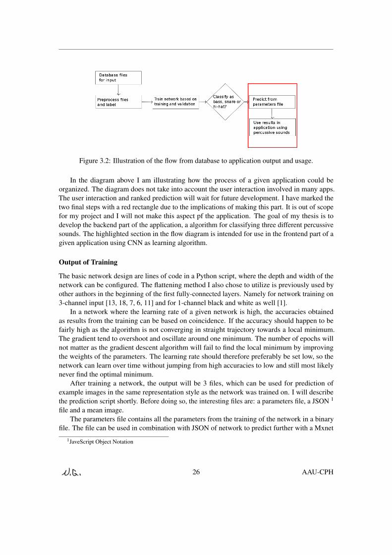
Figure 3.2: Illustration of the flow from database to application output and usage.

In the diagram above I am illustrating how the process of a given application could beorganized. The diagram does not take into account the user interaction involved in many apps.The user interaction and ranked prediction will wait for future development. I have marked thetwo final steps with a red rectangle due to the implications of making this part. It is out of scopefor my project and I will not make this aspect pf the application. The goal of my thesis is todevelop the backend part of the application, a algorithm for classifying three different percussivesounds. The highlighted section in the flow diagram is intended for use in the frontend part of agiven application using CNN as learning algorithm.

Output of Training

The basic network design are lines of code in a Python script, where the depth and width of thenetwork can be configured. The flattening method I also chose to utilize is previously used byother authors in the beginning of the first fully-connected layers. Namely for network training on3-channel input [13, 18, 7, 6, 11] and for 1-channel black and white as well [1].

In a network where the learning rate of a given network is high, the accuracies obtainedas results from the training can be based on coincidence. If the accuracy should happen to befairly high as the algorithm is not converging in straight trajectory towards a local minimum.The gradient tend to overshoot and oscillate around one minimum. The number of epochs willnot matter as the gradient descent algorithm will fail to find the local minimum by improvingthe weights of the parameters. The learning rate should therefore preferably be set low, so thenetwork can learn over time without jumping from high accuracies to low and still most likelynever find the optimal minimum.

After training a network, the output will be 3 files, which can be used for prediction ofexample images in the same representation style as the network was trained on. I will describethe prediction script shortly. Before doing so, the interesting files are: a parameters file, a JSON 1

file and a mean image.The parameters file contains all the parameters from the training of the network in a binary

file. The file can be used in combination with JSON of network to predict further with a Mxnet

1JaveScript Object Notation

26 AAU-CPH

script. This Mxnet script is shown in the Appendix so the reader can get a impression of how thatwould work.

The JSON file is the network in a node format from the input layers, through hidden neuronsto output units. It contains network precisely as it has been setup in a Python script. I willdescribe the Python script and the entire network in the next chapter, together with the variationsof networks I have used to experiment with. Concretely the JSON file can be used in the nextstep of predicting one of the classes from a given example image of the representation used fortraining the CNN.

The mean image is created during running the training, if the network used and the iterator isused to request it. From a visual perspective there is not really anything to realize from this file, asit is binary. Computers read such files perfectly well but humans usually find it hard. Nonetheless,the mean image is also used to in the prediction script. The important thing to realize is that themean image is created as a mean of all images’ pixel values in the training and validation sets.

Input for Prediction

The prediction script is primarily used for image processing using the CNN method and uses anpredefined image shape for the prediction. Due to this constraint I could reprocess the datasetused for testing and use the new dataset representation in the best performing network in order tocomply with original settings of the prediction script.

27 AAU-CPH

Chapter 4

Implementation

The following chapter will describe the full setup of my thesis implementation from preparingdata input, converting to binary files which can be read by the network scripts and finally thenetwork architecture. The structure of my network architecture will be simple and inspired of[2, 3, 5, ?] for making it usable for instrument classification. The foundation of the network isroughly configured utilizing existing setup from [1], which I have found in the Mxnet repository.For the task of training a CNN it is crucial to provide the optimal data as input, based on what areais in focus of the network (e.g. onset detection, sound recognition, image processing, roboticsetc.). The full scripts from where the code snippets in this chapter are taken can be found in theAppendix.

4.1 Data Preparation

This section is dedicated to the data processing before it is being fed into the network as input.In scenarios where sounds are being used, the preprocessing is a vast part of the process. Thenetwork I have created does not recognize raw sound files and have to be converted imagerepresentations for the input. I will use modified spectrograms of the sounds a bass drums,high-hats and snare drums.

4.1.1 MATLAB

In this section I will present essential code snippets used to prepare the dataset from MATLAB.The idea is to show how some of the concepts of normalization, parameters for analysis of thesounds and output are developed.

clear% number of columns to be processeddebugMode=1;noCols=8;noFreq=80;

28

frameRate=100;am=1/6; % amplification factorsplitRatio= 0.8% split rate: portion of training data

quant=256;lowestFrequency=27.5;windowSize=512;

exp_name=’exp4’;jpg_dir=’../drums/’;

data_base_path=’../Nicolai/’data_subdir={’Bass/’,’Hihat/’,’Snare/’};

anaWinSec=1/frameRate*(noCols+2); % in sfile_len_cum=0;for d=1:3, %:2,file_lst=dir([data_base_path data_subdir{d}]);file_len(d)=length(file_lst)-3;file_idx=4:file_len(d);for i=1:file_len(d),[snd,fs]=audioread([data_base_path data_subdir{d} file_lst(i+3).name]);anaWinSmp=ceil(anaWinSec*fs);snd_fr=snd(1:min(size(snd,1),anaWinSmp));amp=am/mean(abs(snd_fr));[dummy dummy earMag{file_len_cum +i}] = mfcc_thesis(amp*snd_fr, ...fs, frameRate,noFreq,lowestFrequency,windowSize);

lab(file_len_cum+i)=d;endfile_len_cum=file_len_cum+file_len(d);

end

%%i=1;j=1;while i<=length(earMag),

if ~isempty(earMag{i}),if size(earMag{i},2) < noCols,sprintf(’%d:col=%d’,i,size(earMag{i},2))

elseif isinf(min(min(earMag{i}))),sprintf(’%d:-inf’,i)

elseif isinf(max(max(earMag{i}))),sprintf(’%d:inf’,i)

elseearMag1(j,:,:)=earMag{i}(:,1:noCols);

29 AAU-CPH

lab1(j)=lab(i);j=j+1

endelsei

endi=i+1;

endclear earMag labearMag=earMag1;lab=lab1;clear earMag1 lab1

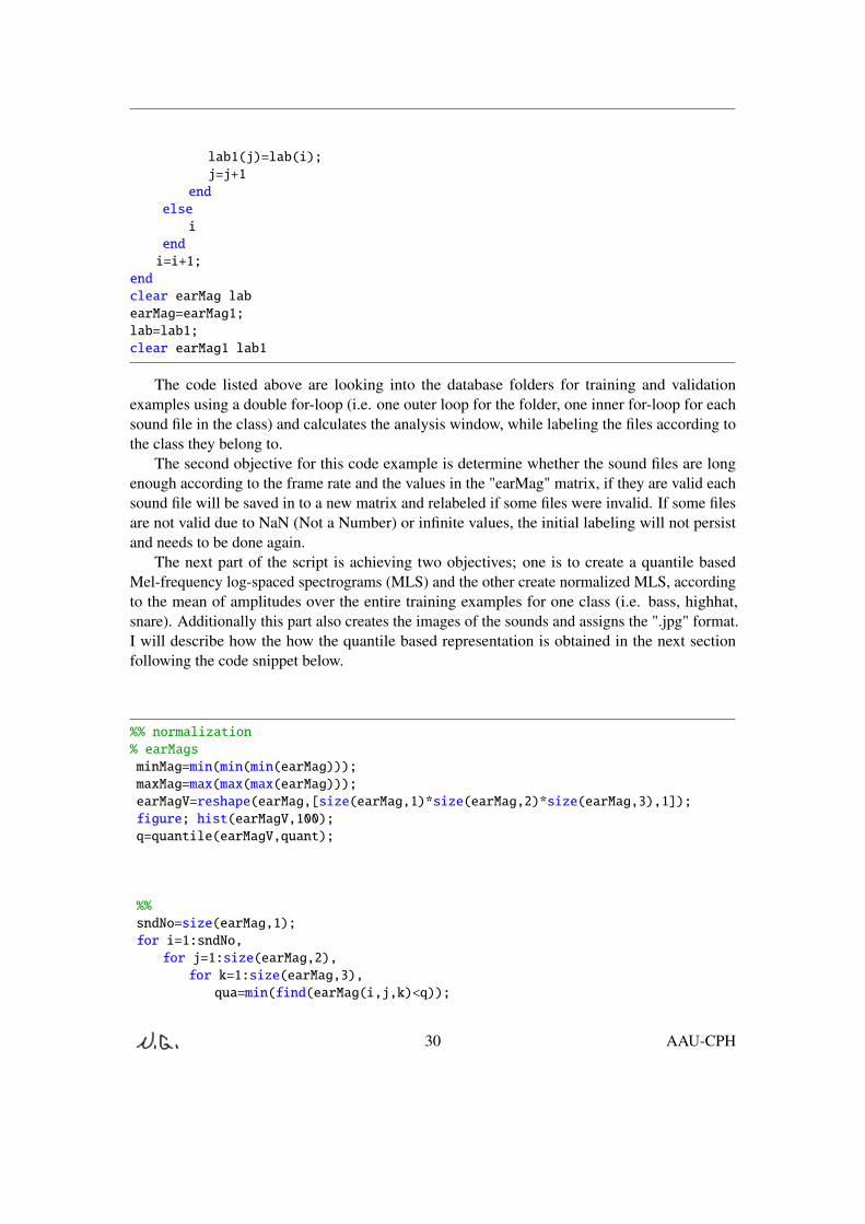
The code listed above are looking into the database folders for training and validationexamples using a double for-loop (i.e. one outer loop for the folder, one inner for-loop for eachsound file in the class) and calculates the analysis window, while labeling the files according tothe class they belong to.

The second objective for this code example is determine whether the sound files are longenough according to the frame rate and the values in the "earMag" matrix, if they are valid eachsound file will be saved in to a new matrix and relabeled if some files were invalid. If some filesare not valid due to NaN (Not a Number) or infinite values, the initial labeling will not persistand needs to be done again.

The next part of the script is achieving two objectives; one is to create a quantile basedMel-frequency log-spaced spectrograms (MLS) and the other create normalized MLS, accordingto the mean of amplitudes over the entire training examples for one class (i.e. bass, highhat,snare). Additionally this part also creates the images of the sounds and assigns the ".jpg" format.I will describe how the how the quantile based representation is obtained in the next sectionfollowing the code snippet below.

%% normalization% earMagsminMag=min(min(min(earMag)));maxMag=max(max(max(earMag)));earMagV=reshape(earMag,[size(earMag,1)*size(earMag,2)*size(earMag,3),1]);figure; hist(earMagV,100);q=quantile(earMagV,quant);

%%sndNo=size(earMag,1);for i=1:sndNo,for j=1:size(earMag,2),for k=1:size(earMag,3),qua=min(find(earMag(i,j,k)<q));

30 AAU-CPH

earMagN(i,j,k)=(earMag(i,j,k)-minMag)/(maxMag-minMag);if isempty(qua),qua=quant;

endquan(i,j,k)=qua-1;

endend

end

%%jpg_path=[jpg_dir exp_name ’/’];jpgN_path=[jpg_dir exp_name ’N/’];

for i=1:sndNo,ima(:,:)=quan(i,:,:);imwrite(ima(:,:)/quant,sprintf(’%sdrum%d.jpg’,jpg_path,i))imaN(:,:)=earMagN(i,:,:);imwrite(imaN(:,:),sprintf(’%sdrum%d.jpg’,jpgN_path,i))

end

%%if debugMode,close all

4.1.2 Quantile Based Representation

Representing the data for time and frequency I perform normalization. For each frequency bandand time frame I rescale the values from 0 to 255. Then calculate the 256 quantiles and assign i asa value, if the value falls between quantile i−1 and i or 0 for the lowest or 255 for the highest. Iwill compare with normalized MLS spectrograms in the beginning of the test chapter to determinethe optimal representation to use for my project.

MFCC Calculation

The MFCCs are calculated in a separate script that is called as a function from the main script Ihave described in the previous section.

for start=0:cols-1first = start*windowStep + 1;last = first + windowSize-1;fftData = zeros(1,fftSize);fftData(1:windowSize) = preEmphasized(first:last).*hamWindow;fftMag = abs(fft(fftData));

31 AAU-CPH

earMag = log10(mfccFilterWeights * fftMag’);

In the code snippet above I show how the absolute FFT magnitude are assigned MFCC filterweights based on the triangular windowing done to the FFT values from the original audio signal.

The figure 4.1 below shows from left to right: A) normalized amplitude, not zero mean and unitvariance, B) then with both zero mean and unit variance plus normalized amplitude, C) thenwithout normalized amplitude but with zero mean and unit variance, lastly D) without zero meanand unit variance and not any normalized amplitude. These instances of representations arecreated before quantiles are calculated.

Figure 4.1: Illustration showing different training examples created in MATLAB from left toright: A), B), C) and D).

Here its visible that the zero mean and unit variance creates entirely different representationthan normalized amplitude and together it has improvement. Furthermore the zero mean and unitvariance applied to single training examples does not influence the output representation. Its hasbeen presented in previous research that zero mean and unit variance are applied, I will questionthat the effects are strong in terms of representation.

The final representation of the sound files is a MLS of normalized amplitude in each trainingexample as shown in figure 4.2.

32 AAU-CPH

Figure 4.2: Illustration showing the final representation of different sounds in the shape 80x8created in MATLAB.

4.1.3 Im2rec Tool

In order to create iterator used for the network, where batch size figures, mean images are created(i.e. mean of all image pixel values for the dataset both training and validation set) and datashape, a tool called im2rec is used. The functionality of the tool is based on files in .lst format.The file is basically a container for image representation index number, label and a path to therepresentation. The tool will convert the .lst file in a .rec file that can be read by the iterator whentraining the network.

A full example file of how the validation set is created using the im2rec tool can been seen inthe Appendix.

4.1.4 Python Scripting

Based on existing scripts located in the Mxnet repository, I have continued working on the script"train_mnist.py" and altered it to the best of my knowledge and competencies within Python.The results are the network architectures before they are converted into JSON files a results of thetraining process and can be used prediction. The scripts from Mxnet have already been structuredwith methods and arguments that can be used when calling the script e.g. learning rate, batch-size,learning rate factor. I have removed what is superficial in order to complete my simulations fromscripts.

train_dataset = ’exp4NTr0.rec’val_dataset = ’exp4NEval0.rec’batch_size = 256#shape = 256

33 AAU-CPH

def get_iterator(data_shape):def get_iterator_impl(args, kv):data_dir = args.data_dir#if ’://’ not in args.data_dir:# _download(args.data_dir)flat = False if len(data_shape) == 3 else True

train = mx.io.ImageRecordIter(path_imgrec = os.path.join(args.data_dir, train_dataset),mean_img = args.data_dir + "trainMIFN_mean.nd",data_shape = data_shape,batch_size = batch_size,rand_crop = True,rand_mirror = True,num_parts = kv.num_workers,part_index = kv.rank)

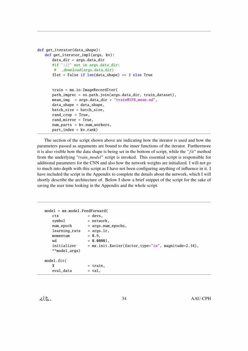
The section of the script shown above are indicating how the iterator is used and how theparameters passed as arguments are bound to the inner functions of the iterator. Furthermoreit is also visible how the data shape is being set in the bottom of script, while the " f it" methodfrom the underlying "train_model" script is invoked. This essential script is responsible foradditional parameters for the CNN and also how the network weights are initialized. I will not goto much into depth with this script as I have not been configuring anything of influence in it. Ihave included the script in the Appendix to complete the details about the network, which I willshortly describe the architecture of. Below I show a brief snippet of the script for the sake ofsaving the user time looking in the Appendix and the whole script.

model = mx.model.FeedForward(ctx = devs,symbol = network,num_epoch = args.num_epochs,learning_rate = args.lr,momentum = 0.9,wd = 0.00001,initializer = mx.init.Xavier(factor_type="in", magnitude=2.34),**model_args)

model.fit(X = train,eval_data = val,

34 AAU-CPH

4.2 The Network Architecture

In this section I will describe in details how the different networks used in my thesis are structured,beginning with what I call my fundamental network. The fundamental CNN is based on ideasinspired by the research in the field and Schlüter et al. among others, with three different variantsof it. These variants are including new and old techniques I have discussed in earlier chapters ofthis report.

One essential element worth mentioning again is the low-level feature representation used inthis work. It is based on 80x8 pixel MLS of the normalized audio files as mentioned in 4.1.1.

Figure 4.3: Illustration showing the fundamental CNN architecture created in the Python script.

4.2.1 Fundamental CNN Variant

After numerous initial experiments of different settings and review loads of research I have chosento use the following setup for my architecture. I have described in the previous design chapter,what have influenced me in making the design and implementation decisions.

The fundamental variant of architecture consist of 3 hidden layers and two fully-connectedlayers. The first input layer is 16 filters of 2x4 convolutional kernels using tanh activationfunctions for the weights, followed by a max-pooling layer of 3x1 and stride 1x1 using ’max’method in the pooling. The second layer is constructed of 32 filters of 3x3 kernels using tanh,followed by max-pooling of 3x1 and stride 1x1. The third and final convolutional layer is 64 filterof 3x3 using tanh and max-pooling of 3x1 and stride 1x1.

35 AAU-CPH

The first fully-connected layer consist of a flattening technique, 256 hidden layer units andactivations functions of tanh. Last fully-connected layer has 3 output units, corresponding to thethree classes using a Softmax classifier for the output.

4.2.2 Network Variants

I have created three different networks using the techniques described earlier. The methods arewidely used in the literature and authors have different suggested results from the use of them.Now I have the chance to do my own testing on these variants.

• Based on the earlier research I have placed the dropout technique in the end of the firstfully-connected layer, before the final fully-connected layer where output units calculatedby a Softmax classifier.

• The batch normalization version of the network will have the technique contained in allconvolutional layers before the activations functions are calculated.

• Dropout and batch normalization combined together in the fundamental network structure.

The script for fundamental network and the listed variations can be found in the Appendix.As a secondary mean for testing scenarios of the implementations, I have also created the

networks using ReLU and sigmoid activation functions. For these I have changed the tanhfunction with ReLU in the three convolutional layers, while changing the first fully-connectedactivation function to sigmoid and maintaining the Softmax classifier for the output.

Now I will proceed to evaluation part of my report containing testing and evaluation.

36 AAU-CPH

Part III

Evaluation

37

Chapter 5

Testing

In this chapter I will go trough the tests and experiments made during this thesis period. I willdescribe how the initial testing have been conducted with my CNNs and my percussive dataset.Moreover the results of experiments related to determining training and validation accuracies willbe presented. The training have been processed on the AAU server, where locally installed CPUsare used to utilize high-performance hardware with the benefit of decreasing computation time.

• The validation accuracy estimates the performance of classification. The cost function usedfor validation accuracy measures how well the neural network algorithm fit the trainingdata.

I will not focus on describing the initial testing of networks in relation to Cifar-10 andImageNet dataset because these utilize the "Inception" network, which train over a long timespan. For the dataset I am using in this thesis, the networks are simply to extensive and advanced.So as I have mentioned earlier, the deeper and the wider a network, the better it will perform isnot true for my dataset. Basically only the deeper network have shown good results compared tothe setup in [1] as I will show shortly and discuss in a later chapter. The width (i.e. numbers offilter for each layer) can decrease the performance.

5.1 Initial Testing

This section will cover the initial testing of different sound representation, the input data shouldselected according to the best performance using the fundamental network. The representationindicating the best results over 300 epochs will be used for further tests in my thesis. Thefollowing subsection will present the results from these experiments and figures as selectionapproach.

5.1.1 Initial experiment quantile MLS vs normalized MLS

In this initial experiment I want to test whether the quantile technique used in the preprocessingstep has an effect on the validation accuracy, compared to the normalized MLS representation.

38

And secondly if there is a difference, if the activation functions in the fundamental network arechanged from consistently using tanh throughout the net. Then to ReLU in the convolutionallayers and sigmoid in the first fully-connected layer as the variations in the previous chapter wassuggested to be composed of.

Testing accuracies of CNN on different representationsDataset: Accuracy % Epoch Learning rateQ-MLS 0.95 299 0.05N-MLS 0.95 299 0.05

Table 5.1: Table showing epoch number and accuracies in percentage of training and validationdata using tanh.

Testing accuracies of CNN on different representationsDataset: Accuracy % Epoch Learning rateQ-MLS (ReLU+sigmoid) 0.49 299 0.05N-MLS (ReLU+sigmoid) 0.84 299 0.05

Table 5.2: Table showing epoch number and accuracies in percentage of training and validationdata using ReLU and sigmoid functions.

The conclusion from this initial experiment ends with choosing the normalized MLS imagerepresentation of the sound files. This preprocessing technique was described in the implementa-tion chapter 4.1.1.

5.2 CNN Testing

In this section I will describe how the testing of the different networks have been conducted. Iwill start by presenting the common parameters such as number of epochs, representation shapeand the dataset.

• The experiments have been stopped after 300 epochs (i.e. starting from 0) and I will thelast epoch’s validation accuracy from the experiment.

• Dataset using 1-channel ranged from 0-255 and image shape of 80x8.

The table below contains details about dataset used for my thesis. The testing results will bebased on this ratio between training and validation set.

39 AAU-CPH

Dataset Structure

Dataset: Training Examples Ratio in Percentage

Training data 2970 80 %Validation data 743 20 %Total 3713 100%

Table 5.3: Table showing dataset divided into training and validation data.

Proceeding to the actual testing scenarios I will introduce the performed experiment and theresults hereof.

5.2.1 Testing Different Learning Rate on CNN with N-MLS

In this experiment I want to test whether of the CNN performs best in validation accuracy,using a static learning rate for each group of experiment iterations and tanh activation functionsthroughout the networks. The third column in the table will indicate the learning rate used fornetwork training.

Test results of the different CNN

CNN: Accuracy Epoch Learning rate

Fundamental 0.95 299 0.05Fundamental + Dropout 0.96 299 0.05Fundamental + BN 0.97 299 0.05Fundamental 0.95 299 0.005Fundamental + Dropout 0.95 299 0.005Fundamental + BN 0.97 299 0.005

Table 5.4: Table showing epoch number and accuracies in percentage of training and validationdata.

The network scoring highest in validation accuracy is the fundamental network with BNapplied. This is the case in both iterations using this network regardless of the learning rate.

Next I will go into details with a new experiments using a similar approach for iterations.

5.2.2 Testing Different Learning Rates on CNN with N-MLS implementing ReLUand Sigmoid

In this experiment I want to test whether of the CNN performs best in validation accuracy. Againwith different but static learning rates. Furthermore the networks architecture is modified to haveReLU and sigmoid activation function implemented.

40 AAU-CPH

Test results of the different CNN and activation

CNN: Accuracy Epoch Learning rate

Fundamental 0.84 299 0.05Fundamental + Dropout 0.74 299 0.05Fundamental + BN 0.98 299 0.05Fundamental 0.95 299 0.005Fundamental + Dropout 0.96 299 0.005Fundamental + BN 0.97 299 0.005

Table 5.5: Table showing epoch number and accuracies in percentage of training and validationdata.

It is clear from the metrics of validation accuracy in the table above that fundamental net withBN outperforms other network variants. With a learning rate of 0.05 the fundamental net withBN performs extremely well. The accuracy is 14 % higher than the next best net structure, beingthe fundamental net.

Finally, a last experiment have been conducted in order to investigate how the dropout and BNwould perform together in the fundamental network. The learning rate chosen for this scenario isbased on the higher average from earlier experiments using ReLU and sigmoid activations.

5.2.3 Fundamental CNN with Batch Normalization and Dropout on NormalizedMLS

In this experiment I want to test whether the BN and dropout together has an effect on thefundamental CNN and improves the validation accuracy beyond what the fundamental with BNresults in.

Testing accuracies of CNN on different representationsCNN: Accuracy % Epoch Learning rateFundamental + BN + Dropout 0.97 299 0.005

Table 5.6: Table showing epoch number and accuracies in percentage of training and validationdata

The validation accuracy from this experiment is 97 %.In the next chapter I will evaluate on these results and compare the different experiments,

including the variation of networks.

41 AAU-CPH

Chapter 6

Evaluating the Results

In this chapter the results presented in the previous chapter will be evaluated. I will evaluate basedon validation accuracy as metric. I will treat the validation accuracy as the estimated probabilitythat my network will be able to predict the correct class label. I will also look into how the resultscompares to other contributions to the field of CNN for instrument classification.

6.1 Test Evaluation

In this section I will discuss the results from the previous chapter and observations made duringthe experimentation. Furthermore I will go into what parameters presented in the analysis chapter2, which might have influenced the results. A more elaborate discussion of the parameters for theCNN can be read in the next chapter.

• Learning rate

• Activation Functions

• Batch Size

• Kernel Sizes

• Amount of Filters

• Batch Normalization

• Dropout

• Image Representation

• Network Depth and Width

The parameters mentioned in bullets above are all items that can affect the performanceof the network. In the design chapter I have already starting picking out the parameters foundreasonable to use in the implementation of my network. I will elaborate on all these parameters

42

in the discussion chapter following this evaluation of the test results. While in this chapter I willfocus mainly of learning rate, activation functions, dropout and batch normalization, since theywere the primary parameters and conditions to test.

6.1.1 Fundamental Network

The first network I call my fundamental network have been scoring at a validation accuracy of 95% in the experiment using tanh functions regardless of the learning rate used. When consideringthe amount of epochs used (i.e. 300) it can be interpreted as an indication that the network havereached the upper accuracy limit for the net. Meaning that the low learning rate of 0.005 managesto converge at the local minimum the same as learning rate of 0.05 after many epochs. Now, if thefinal epoch with learning rate of 0.005 did not achieve the same accuracy as with 0.05, I mighthave suspected that the lower learning rate was slower to converge and hereby also should usemore computational time in order for the gradient descent to converge for the cost function.

The next experiment involving the fundamental structure was based on a different computa-tion for the weights of net. The activation functions was changed and using the higher learningrate of 0.05 the network performed 2nd best of the three nets compared. The low validationaccuracy could indicate that the gradient descent was overfitting and had trouble converging atthe local minimum. Another case would simply be that the algorithm had to use more epochs forreaching a higher accuracy score, which I consider less likely to ever happen when looking atmetrics for a lower learning rate. Using a lower learning rate the network achieved even better at0.95, making me wonder why the activation functions of ReLU and sigmoid may have caused thehigher learning rate to overfit due to calculated weights that were not improving accuracy overtime.

6.1.2 Dropout Network

Returning to the first experiment using tanh activations in the network while having dropoutapplied I have found a higher accuracy for the network with learning rate of 0.05 (i.e. 96 %).The case of overfitting might have been reduced slightly in this network, when looking at thefundamental network and thus improved the algorithm using dropout. The reason for the loweraccuracy in the experiment with low learning could indicate that the algorithm in this case wouldbenefit from more epochs to train. On the contrary the results can also be a coincidence andsimply an expression of insignificant difference between the two different learning rates for thenetwork.

Continuing to the next experiment with changed activation functions a similar reduction canbe seen for the dropout network using a high learning rate. The network perform least goodand scores a accuracy of 74 %, which is quite a big difference compared to the experimentdescribed before. In this case the activation functions might have calculated the weights for thegradient descent in the units hidden layers less optimal and when the dropout techniques alsorandomly removes results from the layers to the next units. This can cause the algorithms to seemextraordinary bad. Using a lower learning rate, the network performs better despite the activation

43 AAU-CPH

functions applied, giving an indication that the algorithm was calculating wrong weights for thenetwork using the high learning rate. Lastly, a solution could also be to use more epochs than the300 used and hope for a higher accuracy with high learning rate. I consider this as a very doubtfulsolution because the network using a lower learning rate have seemed to score high. More likelythe high learning causes the activation functions to calculate weights wrongly for the gradientdescent and overfits.

6.1.3 Batch Normalization Network

Evaluating the final network included in the iterations of experiments indicates improvementof the algorithm variations. The network with BN scored the highest validation accuracy in allexperimental variations, 97 % in both with high and low learning rate with tanh activations. Theresults seem to agree with the advantages of BN mentioned in [5] and section 2.5 of my thesis.Applying BN diminishes the need for selecting a learning rate that is high or low in order toachieve good performance for the CNN.

The next iteration of experiments using ReLU and sigmoid indicates the same superior per-formance by the network. Though it might seem hard to evaluate why the results are so differentin the high learning rate condition compared to the other network variants. One suggested expla-nation is that the BN net is not affected by the disadvantage of having hidden layers randomlyremoved during convergence of the gradient descent. Additionally, as the network appears tobe independent of high or low learning rate, the network can even perform better using theseactivations than with tanh. Consequently this could suggest, that the activations are not calculatingweights that are wrong during training. With lower learning rate the network performs equallywell as in other settings and this suggest that the network have converged at the local minimum inevery iteration and condition. Optionally more epochs could be used in order to look for betterperformance. The validation accuracy was observed to be increased steadily and most likely itcan achieve a higher accuracy if using more epoch for testing the algorithm.

As I have discussed previously in section 2.5 the technique is based on decreasing thecovariate shift when training a deep neural net. Since the network here used in the previous testsettings is not very deep and/or wide, the covariate shift might not be a problem as such.

6.1.4 Combined Dropout and Batch Normalization

The last experiment for my thesis is looking for further improvement in the fundamental network,specifically using both dropout and BN to achieve higher accuracy than any of the existingvariants. The results was an accuracy of 97 % resembling the accuracy of the fundamentalnetwork with BN. From this perspective there simply is not indication that dropout and BNtogether would improve the fundamental network more than BN could do on its own.

44 AAU-CPH

6.2 Subconclusion

The fundamental network did not perform different when having high and low learning rate. Thenetwork did decrease in accuracy though when the activation function was changed to ReLUand sigmoid, while maintaining a high learning rate. The network with dropout performed betteror equal to the fundamental network in the experiments with tanh activations, using high andlow learning rate respectively. With changed activations the dropout network decreased a lotcompared to other networks with the same high learning rate. When changing the learning rate tolow, the network returned to competitive high validation accuracy. BN appeared to perform betterthan other networks in these experiments, not dependent of learning rate nor activation functions.Finally the fundamental network combined with dropout and BN together, performed the sameas a network with BN alone when using a low learning rate. I will argue that the network testedand evaluated here are competitive to some extent (see figure 2.2 and section 1.1.1 for previousresults) with recent research in both onset detection, image-recognition tasks and instrumentclassification. Only in some situations the network fails and score low in validation accuracies.

45 AAU-CPH

Part IV

Finalization

46

Chapter 7

Discussion

In order to discuss the content and new insights of my project somewhat systematically I willdivide this chapter into section, where I can elaborate on the network parameters and generalissues I have found interesting from my thesis. There are many aspect of the report that could getmore attention and be discussed to a large extent. I have asserted most of my work and selectedwhat I find most urgent.

The contribution of this report relies on I have chosen to present results from the experimentsof my work and my findings, despite other promising results are shown by [4], since they usea different input approach for the network. When using two different inputs (MRP, MLS), thetime used for preprocessing will surely increase compared to using one input and it can be moreprone to human or computational errors. In the study made in [20] the authors test their CNNimplementation with raw audio data. The accuracy results from their best performing modelsare not impressive compared to other results in the field. Furthermore the authors suggestedto investigate further the inner workings of the CNN filter weights and transformations causedby the network. In my project I have used a fundamental sound representation in form of theMLS. The parameters of the spectrogram have only been enhanced by MFCC filter weightsand normalized in amplitude but otherwise it is simple and easy to use in a CNN. The CNNhave lots of parameters already that can influence the performance of the algorithm, so in myopinion it is crucial to limit the amount of input features. My findings show that the simple input(only MLS using one input channel) can produce competitive results. And especially differentnetwork architecture and techniques for improving the performance by changing the internalstructure have been of interest to me. The previously mentioned research [4, 20] have show theirresults on a given model with parameters, without showing results from experimenting withdifferent internal settings for learning rates, activations functions and recent new advances such asbatch normalization. Additionally how well a CNN will adapt to mixture of acoustic and digitalrecordings in a long-time gathered database.

47

7.1 Network Parameters

From the research I have done in the beginning of this project I learned about a lot of differenttechniques and ways to alter the neural networks. This being preprocessing of input featuresfor the network, different mathematical functions for calculating weights between layers in thenetwork to suggested methods developed for dataset of millions of image and classification hereof.The first parameter for my CNN that I want to discuss is learning rate.

7.1.1 Learning Rate

From the experiments described in this report, its obvious that parameters has influenced onhow well the weights of the gradient descent will be updated during training. Especially for ahigh learning rate, the network had difficulties with convergence when using ReLU and sigmoidfunctions.

The learning rate has in this project been variated in a factor of 10. It is not easy to predictwhether a network will perform better or worse if learning rate is the only parameter beingchanged. The performance affected learning rate will certainly depend on activation functionsused as seen in the testing, network depth and batch size.

7.1.2 Activation Functions

The mathematical function used in forward propagation (and backpropagation) of CNN forcalculating the weights for the units in the hidden layers have shown to have little influence on theresults in my thesis and the experiments. Only in combination with a too high learning rate thenetwork have been affected. The network using dropout and high learning rate scored extremelybad in one iteration of the test, suggesting that the activation functions output for the filters areclosely related and does not benefits from loosing weights connecting the layers.

7.1.3 Batch Size

The batch size have several implications, if it is too small the network will not train very well. Ifthe batch size is small, it has been useful to have a higher learning rate than 0.05 approaching 0.5.The research in the field expose batch sizes from 16-256 and I found that 256 is appropriate forthe type of gradient descent used in this thesis. The batch size will depend on whether applyingSGD and MBGD, nowadays many networks use a MBGD like approach, since it is faster thantraditional GD. It my situation the networks using BN have been affected positively by normalizedthe input to each layer by having zero mean and unit variance for each mini-batch. Contradictingwas I have earlier suggested in section 4.1.1; zero mean and unit not having influence on the MLSrepresentation of the audio. The results from testing indicate that the BN, which implies zeromean and unit does have a positive effect on the validation accuracies.

7.1.4 Number of Filters

The number of filters in every layer have shown to affect the performance, if too many filter areused, computational cost will increase and it is not a guarantee performance metrics will increase

48 AAU-CPH

together with the amount of filters. It is also well-known that many modern convolutional network[13, 7, 11, 6] like the ones used in on ImageNet datasets are training over several weeks and usingmultiple GPUs for the task.

7.1.5 Depth of Network

Quite frequently the related literature present networks as improving when the size of the networkis big. From the research made here, it can have some truth to the matter. As Lecun et al. usedtwo convolutional layer for their database of 60000 images and 10 outputs, I have increased mynetwork with one additional layer and still achieved high accuracy scores. On the contrary I havementioned in the previous section that applying too many feature maps or filter to each layer,will not benefit the algorithms performance in terms of validation accuracy. The width of thenetwork cannot be expanded without loss in validation accuracies and the reason for that couldbe answered by comparing it to having a high learning rate. The gradient descent will overshootand not converge at any optimal minimum.

7.1.6 Filter Kernels

The dimensions of the filter kernel are hard to determine but there should be coherence betweeninput image representation and the sizes of convolutional kernel and max-pooling kernel. Variousproblem have occured in my implementations if the stride was higher that 1x1 and causedmismatch between image shape and the kernel sizes chosen. In early experiments using smallerkernels than the ones presented for the first convolutional layers, the batch normalization trainingprogress appeared unstable and the validation accuracies varied widely from one epoch to thenext. Suddenly during the training, the accuracy for one epoch is 0.84 and then it drop to 0.56and then back to 0.83.

It is evident that the kernel dimensions are important for the training to progress smoothlyand not affect overshooting.

7.2 Network Variants

In this final section before the conclusion I want to reflect on the concepts I have used in theexperiments for the variants. Not the internal parameters and architecture as such, rather the newmethod in the field that I have been experimenting with.

7.2.1 Dropout

Depending on the learning rate parameter and activation function combination, the dropouttechniques will enhance the performance of a network. Its not always beneficial to randomlydrop 50 % of the units in the hidden layers, it will surely keep a acceptable training speed ofthe network. As consequence the gradient descent will not be provided with the optimal filtersweights when updating the kernels for convolution.

49 AAU-CPH

7.2.2 Batch Normalization

Increases the computation time for a network with double of the time for dropout networks ornetwork using neither dropout og BN, which might be the only negative issue to focus on of thisapproach. BN appears to be independent of learning rate and the validation accuracy is high in allconditions of experiments done. This scores the highest accuracy and ensures that the learningrate will not affect the convergence with respect to the gradient descent and filter weights.

7.2.3 Observations

The data used from the database contain both digital and acoustic recordings. This can influencethe performance of the algorithms, since the waveforms of sounds in digital and acoustic formatare very different.

During training of different networks in the initial phase, before deciding the fundamentalnetwork architecture. I have observed some cases where the validation accuracy was high, whilethe training error was much lower. I perceived this as a sign of overfitting or underfitting, meaningthat my algorithm was suffering from high variance. Then I started implementing different typesof normalization to the amplitude of my training examples and the two accuracy metrics startedaligning much better.

Including the mean image in the iterator improves learning tremendously. Before applyingthe mean image the algorithms will not perform well and score approximately at random accuracyof predicting the correct labels for the classes.

Stopping training after 300 epochs for each experiment variant due to time constraints. Insome network variants (e.g. fundamental with BN and the fundamental with dropout and BN) thevalidation accuracies could increase from their current scores.

50 AAU-CPH

Chapter 8

Conclusion

As a final conclusion to my thesis I will present a short review of important aspects. Startingwith research in field where I found useful information about neural networks and CNNs ingeneral. This provided a fine impression to how the networks are combined of different mathalgorithms for forward propagation, backpropagation and calculating weights. I defined myclassification problem as involving percussive sounds and a objective of multi-class output.Among the requirements for creating a network, I realized that normalization was a crucialpart of final representation output for the input unit in the CNN. The learning rate was alsoand important parameter to be aware of, depending on which other architectural elements wasotherwise used. Here I think of activation functions that showed to be influenced by the learningrate in experiments.

I suggested a overall design for an application utilizing the backend programming I havedeveloped in Python and chose initial settings for the training process. The important part of theapplication is the possibility to predict the correct labels for each percussive sound comprisingthe dataset. I have been using bass, snare and high-hat as my percussive instruments. The usedmetric for measuring how well these labels were predicted later showed acceptable results.

The implementation consisted of several steps, for the preprocessing of the dataset, labeling,MFCC calculation, normalization of MLS and separation of dataset into training and validationsets, among others. Next, I created the iterator for the network and the network itself from threeconvolutional layers with max-pooling. I used to fully-connected layers and a Softmax classifierfor the output. I wanted to have different variants for the fundamental network to test for differentresults, after numerous initial test with trial and error. This ended in creating several networks,one with dropout, one with BN and one with a combination of the dropout and BN. I also lookedinto how high and low learning rate would influence the results of the variants. To extent thetesting, I also changed activation functions during the test iterations. The variants performed verysimilar during experiments.

Only the network with BN proved to perform well, regardless of the changes to the learningrate or activations. The combination of ReLU, sigmoid and high learning rate (i.e. 0.05) reallysurprised for fundamental network with BN and performed at 98 % in validation accuracy.

I have discussed many of the parameters and concepts used in testing of my networks frominitial tests to final experiments. I have done this is somewhat systematic fashion in order to

51

assure transparency for improvements and drawbacks of my approach to changing my CNNs.

52 AAU-CPH

Bibliography

[1] LeCun, Y., Boser, B., Denker, J. S., Henderson, D., Howard, R. E., Hubbard, W., & Jackel,L. D. (1989). Backpropagation applied to handwritten zip code recognition,Neural computation, 1(4), 541-551.

[2] Schlüter, J., & Böck, S. (2013). Musical onset detection with convolutional neural networks.In 6th International Workshop on Machine Learning and Music (MML),Prague, Czech Republic.

[3] Schlüter, J., & Böck, S. (2014, May). Improved musical onset detection with convolutionalneural networks. In Acoustics, Speech and Signal Processing (ICASSP),2014 IEEE International Conference on (pp. 6979-6983).

[4] Park, T., & Lee, T. (2015). Musical instrument sound classification with deep convolutionalneural network using feature fusion approach,arXiv preprint arXiv:1512.07370.

[5] Ioffe, S., & Szegedy, C. (2015). Batch normalization: Accelerating deep network trainingby reducing internal covariate shift,arXiv preprint arXiv:1502.03167.

[6] Szegedy, C., Liu, W., Jia, Y., Sermanet, P., Reed, S., Anguelov, D., ... & Rabinovich, A.(2015). Going deeper with convolutions,In Proceedings of the IEEE Conference on Computer Vision and Pattern Recognition (pp.1-9).

[7] He, K., Zhang, X., Ren, S., & Sun, J. (2015). Deep Residual Learning for Image Recognition,arXiv preprint arXiv:1512.03385.

[8] Bishop, C. M. (1995). Neural networks for pattern recognition,Oxford University Press.

[9] Ripley, B. D. (2007). Pattern recognition and neural networks,Cambridge University Press.

[10] Venables, W. N., & Ripley, B. D. (2013). Modern applied statistics with S-PLUS,Springer Science & Business Media.

53

[11] Szegedy, C., Vanhoucke, V., Ioffe, S., Shlens, J., & Wojna, Z. (2015). Rethinking theInception Architecture for Computer Vision,arXiv preprint arXiv:1512.00567.

[12] Zeiler, M. D., & Fergus, R. (2014). Visualizing and understanding convolutional networks,In Computer vision–ECCV 2014 (pp. 818-833). Springer International Publishing.

[13] Krizhevsky, A., Sutskever, I., & Hinton, G. E. (2012). Imagenet classification with deepconvolutional neural networks,In Advances in neural information processing systems (pp. 1097-1105).

[14] Piczak, K. J. (2015, September). Environmental sound classification with convolutionalneural networks,In Machine Learning for Signal Processing (MLSP), 2015 IEEE 25th International Work-shop on (pp. 1-6). IEEE.

[15] Ullrich, K., Schlüter, J., & Grill, T. (2014). Boundary Detection in Music Structure Analysisusing Convolutional Neural Networks,In ISMIR (pp. 417-422).

[16] Grill, T., & Schluter, J. (2015, August). Music boundary detection using neural networks onspectrograms and self-similarity lag matrices,In Signal Processing Conference (EUSIPCO), 2015 23rd European (pp. 1296-1300). IEEE.

[17] Grill, T., & Schlüter, J. (2015). Music Boundary Detection Using Neural Networks onCombined Features and Two-Level Annotations,In Proceedings of the 16th International Society for Music Information Retrieval Conference(ISMIR 2015), Malaga, Spain.

[18] Simonyan, K., & Zisserman, A. (2014). Very deep convolutional networks for large-scaleimage recognition,arXiv preprint arXiv:1409.1556.

[19] Virtanen, T., Gemmeke, J. F., Raj, B., & Smaragdis, P. (2015). Compositional Models forAudio Processing: Uncovering the structure of sound mixtures,Signal Processing Magazine, IEEE, 32(2), 125-144.

[20] Li, P., Qian, J., & Wang, T. (2015). Automatic Instrument Recognition in Polyphonic MusicUsing Convolutional Neural Networks,arXiv preprint arXiv:1511.05520.

[21] Han, J., & Moraga, C. (1995). The influence of the sigmoid function parameters on thespeed of backpropagation learning,In From Natural to Artificial Neural Computation (pp. 195-201). Springer Berlin Heidelberg.

[22] Benetos, E., Kotti, M., & Kotropoulos, C. (2006, May). Musical instrument classificationusing non-negative matrix factorization algorithms,

54 AAU-CPH

In Circuits and Systems, 2006. ISCAS 2006. Proceedings. 2006 IEEE International Sympo-sium on (pp. 4-pp).

[23] Karayev, S., Trentacoste, M., Han, H., Agarwala, A., Darrell, T., Hertzmann, A., & Win-nemoeller, H. (2013). Recognizing image style,arXiv preprint arXiv:1311.3715.

[24] Szegedy, C., Ioffe, S., & Vanhoucke, V. (2016). Inception-v4, inception-resnet and theimpact of residual connections on learning,arXiv preprint arXiv:1602.07261.

[25] https://github.com/dmlc/mxnet,[Last accessed: the 22th of May 2016].

[26] https://www.coursera.org/learn/machine-learning/,[Last accessed: the 5th of May 2016].

55 AAU-CPH

Part V

Appendix

56

Appendix A

The Prediction Script

The following appendix shows the full prediction file in Python. The script is using in theapplication to determine what class a sound belongs to.

import sys, oscurr_path = os.path.dirname(os.path.abspath(os.path.expanduser(__file__)))sys.path.append("../../../amalgamation/python/")sys.path.append("../../../python/")

from mxnet_predict import Predictor, load_ndarray_fileimport mxnet as mximport loggingimport numpy as npfrom skimage import io, transform

# Load the pre-trained model

symbol_file ="//users/STUDENT/ngajhe10/model_inception-BN/mnistThesisFNBNDs-0-0001.params"

param_file ="/users/STUDENT/ngajhe10/model_inception-BN/ImnistThesisFNBNDs-0-symbol.json"

predictor = Predictor(open(symbol_file).read(),open(param_file).read(),{’data’:(1,3,224,224)})

mean_img =load_ndarray_file(open("/users/STUDENT/ngajhe10/model_inception-BN/mean_224.nd").read())["mean_img"]

synset = [l.strip() for l inopen(’/users/STUDENT/ngajhe10/model_inception-BN/synset.txt’).readlines()]

def PreprocessImage(path, show_img=False):# load imageimg = io.imread(path)print("Original Image Shape: ", img.shape)

57

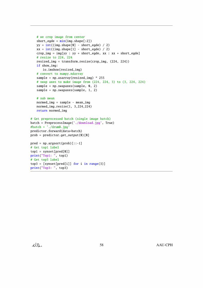
# we crop image from centershort_egde = min(img.shape[:2])yy = int((img.shape[0] - short_egde) / 2)xx = int((img.shape[1] - short_egde) / 2)crop_img = img[yy : yy + short_egde, xx : xx + short_egde]# resize to 224, 224resized_img = transform.resize(crop_img, (224, 224))if show_img:io.imshow(resized_img)

# convert to numpy.ndarraysample = np.asarray(resized_img) * 255# swap axes to make image from (224, 224, 3) to (3, 224, 224)sample = np.swapaxes(sample, 0, 2)sample = np.swapaxes(sample, 1, 2)

# sub meannormed_img = sample - mean_imgnormed_img.resize(1, 3,224,224)return normed_img

# Get preprocessed batch (single image batch)batch = PreprocessImage(’./download.jpg’, True)#batch = ’./drumB.jpg’predictor.forward(data=batch)prob = predictor.get_output(0)[0]

pred = np.argsort(prob)[::-1]# Get top1 labeltop1 = synset[pred[0]]print("Top1: ", top1)# Get top5 labeltop3 = [synset[pred[i]] for i in range(3)]print("Top3: ", top3)

58 AAU-CPH

Appendix B

The Network Script with FundamentalStructure

The following appendix shows the full network file for my architecture (Variant no. 1) in Python.The script is using in the application to train the classifier and for comparison.

import find_mxnetimport mxnet as mximport argparseimport os, sysimport train_model2

def get_lenet():data = mx.symbol.Variable(’data’)# first convconv1 = mx.symbol.Convolution(data=data, kernel=(2,4), num_filter=16)tanh1 = mx.symbol.Activation(data=conv1, act_type="tanh")pool1 = mx.symbol.Pooling(data=tanh1, pool_type="max",

kernel=(3,1), stride=(1,1))# second convconv2 = mx.symbol.Convolution(data=pool1, kernel=(3,3), num_filter=32)tanh2 = mx.symbol.Activation(data=conv2, act_type="tanh")pool2 = mx.symbol.Pooling(data=tanh2, pool_type="max",

kernel=(3,1), stride=(1,1))# third convconv3 = mx.symbol.Convolution(data=pool2, kernel=(3,3), num_filter=64)tanh3 = mx.symbol.Activation(data=conv3, act_type="tanh")pool3 = mx.symbol.Pooling(data=tanh3, pool_type="max",

kernel=(3,1), stride=(1,1))# first fullcflatten = mx.symbol.Flatten(data=pool3)fc1 = mx.symbol.FullyConnected(data=flatten, num_hidden=256)tanh3 = mx.symbol.Activation(data=fc1, act_type="tanh")

# second fullc

59

fc2 = mx.symbol.FullyConnected(data=tanh3, num_hidden=3)# losslenet = mx.symbol.SoftmaxOutput(data=fc2, name=’softmax’)return lenet

train_dataset = ’exp4NTr0.rec’val_dataset = ’exp4NEval0.rec’batch_size = 256#shape = 256

def get_iterator(data_shape):def get_iterator_impl(args, kv):data_dir = args.data_dir#if ’://’ not in args.data_dir:# _download(args.data_dir)flat = False if len(data_shape) == 3 else True

train = mx.io.ImageRecordIter(path_imgrec = os.path.join(args.data_dir, train_dataset),mean_img = args.data_dir + "trainMIFN_mean.nd",data_shape = data_shape,batch_size = batch_size,rand_crop = True,rand_mirror = True,num_parts = kv.num_workers,part_index = kv.rank)

val = mx.io.ImageRecordIter(path_imgrec = os.path.join(args.data_dir, val_dataset),mean_img = args.data_dir + "valMIFN_mean.nd",rand_crop = False,rand_mirror = False,data_shape = data_shape,batch_size = batch_size,num_parts = kv.num_workers,part_index = kv.rank)

return (train, val)return get_iterator_impl

def parse_args():parser = argparse.ArgumentParser(description=’train an image classifer on

mnist’)parser.add_argument(’--network’, type=str, default=’mlp’,

choices = [’mlp’, ’lenet’],help = ’the cnn to use’)

parser.add_argument(’--data-dir’, type=str, default=’mnist/’,

60 AAU-CPH

help=’the input data directory’)parser.add_argument(’--gpus’, type=str,

help=’the gpus will be used, e.g "0,1,2,3"’)parser.add_argument(’--num-examples’, type=int, default=60000,

help=’the number of training examples’)parser.add_argument(’--batch-size’, type=int, default=128,

help=’the batch size’)parser.add_argument(’--lr’, type=float, default=0.005,

help=’the initial learning rate’)parser.add_argument(’--model-prefix’, type=str,

help=’the prefix of the model to load/save’)parser.add_argument(’--num-epochs’, type=int, default=10,

help=’the number of training epochs’)parser.add_argument(’--load-epoch’, type=int,

help="load the model on an epoch using the model-prefix")parser.add_argument(’--kv-store’, type=str, default=’local’,

help=’the kvstore type’)parser.add_argument(’--lr-factor’, type=float, default=1,

help=’times the lr with a factor for every lr-factor-epochepoch’)

parser.add_argument(’--lr-factor-epoch’, type=float, default=1,help=’the number of epoch to factor the lr, could be .5’)

return parser.parse_args()

if __name__ == ’__main__’:args = parse_args()

if args.network == ’mlp’:data_shape = (784, )net = get_mlp()

else:data_shape = (1, 80, 8)net = get_lenet()

# traintrain_model2.fit(args, net, get_iterator(data_shape))

61 AAU-CPH

Appendix C

The Network Script with Dropout

The following appendix shows the full network file for my architecture (Variant no. 2) in Python.The script is using in the application to train the classifier and compare to other network results.

import find_mxnetimport mxnet as mximport argparseimport os, sysimport train_model2

def get_lenet():

data = mx.symbol.Variable(’data’)# first convconv1 = mx.symbol.Convolution(data=data, kernel=(2,4), num_filter=16)tanh1 = mx.symbol.Activation(data=conv1, act_type="relu")pool1 = mx.symbol.Pooling(data=tanh1, pool_type="max",

kernel=(3,1), stride=(1,1))# second convconv2 = mx.symbol.Convolution(data=pool1, kernel=(3,3), num_filter=32)tanh2 = mx.symbol.Activation(data=conv2, act_type="relu")pool2 = mx.symbol.Pooling(data=tanh2, pool_type="max",

kernel=(3,1), stride=(1,1))# third convconv3 = mx.symbol.Convolution(data=pool2, kernel=(3,3), num_filter=64)tanh3 = mx.symbol.Activation(data=conv3, act_type="relu")pool3 = mx.symbol.Pooling(data=tanh3, pool_type="max",

kernel=(3,1), stride=(1,1))# first fullcflatten = mx.symbol.Flatten(data=pool3)fc1 = mx.symbol.FullyConnected(data=flatten, num_hidden=256)tanh3 = mx.symbol.Activation(data=fc1, act_type="sigmoid")dropout2 = mx.symbol.Dropout(data=tanh3, p=0.5)

# second fullc

62

fc2 = mx.symbol.FullyConnected(data=dropout2, num_hidden=3)# losslenet = mx.symbol.SoftmaxOutput(data=fc2, name=’softmax’)return lenet

train_dataset = ’exp4NTr0.rec’val_dataset = ’exp4NEval0.rec’batch_size = 256#shape = 256

def get_iterator(data_shape):def get_iterator_impl(args, kv):data_dir = args.data_dir#if ’://’ not in args.data_dir:# _download(args.data_dir)flat = False if len(data_shape) == 3 else True

train = mx.io.ImageRecordIter(path_imgrec = os.path.join(args.data_dir, train_dataset),mean_img = args.data_dir + "trainMID_mean.nd",data_shape = data_shape,batch_size = batch_size,rand_crop = True,rand_mirror = True,num_parts = kv.num_workers,part_index = kv.rank)

val = mx.io.ImageRecordIter(path_imgrec = os.path.join(args.data_dir, val_dataset),mean_img = args.data_dir + "valMID_mean.nd",rand_crop = False,rand_mirror = False,data_shape = data_shape,batch_size = batch_size,num_parts = kv.num_workers,part_index = kv.rank)

return (train, val)return get_iterator_impl

def parse_args():parser = argparse.ArgumentParser(description=’train an image classifer on

mnist’)parser.add_argument(’--network’, type=str, default=’mlp’,

choices = [’mlp’, ’lenet’],help = ’the cnn to use’)

parser.add_argument(’--data-dir’, type=str, default=’mnist/’,

63 AAU-CPH

help=’the input data directory’)parser.add_argument(’--gpus’, type=str,

help=’the gpus will be used, e.g "0,1,2,3"’)parser.add_argument(’--num-examples’, type=int, default=60000,

help=’the number of training examples’)parser.add_argument(’--batch-size’, type=int, default=128,

help=’the batch size’)parser.add_argument(’--lr’, type=float, default=0.005,

help=’the initial learning rate’)parser.add_argument(’--model-prefix’, type=str,

help=’the prefix of the model to load/save’)parser.add_argument(’--num-epochs’, type=int, default=10,

help=’the number of training epochs’)parser.add_argument(’--load-epoch’, type=int,

help="load the model on an epoch using the model-prefix")parser.add_argument(’--kv-store’, type=str, default=’local’,

help=’the kvstore type’)parser.add_argument(’--lr-factor’, type=float, default=1,

help=’times the lr with a factor for every lr-factor-epochepoch’)

parser.add_argument(’--lr-factor-epoch’, type=float, default=1,help=’the number of epoch to factor the lr, could be .5’)

return parser.parse_args()

if __name__ == ’__main__’:args = parse_args()

if args.network == ’mlp’:data_shape = (784, )net = get_mlp()

else:data_shape = (1, 80, 8)net = get_lenet()

# traintrain_model2.fit(args, net, get_iterator(data_shape))

64 AAU-CPH

Appendix D

The Network Script with BatchNormalization in All ConvolutionalLayers

The following appendix shows the full network file for my architecture (Variant no. 4) in Python.The script is used in the application to train the classifier and compare to other network validationaccuracies.

import find_mxnetimport mxnet as mximport argparseimport os, sysimport train_model2

def get_lenet():name=Nonesuffix=’’data = mx.symbol.Variable(’data’)# first convconv1 = mx.symbol.Convolution(data=data, kernel=(2,4), num_filter=16)bn = mx.sym.BatchNorm(data=conv1, name=’%s%s_batchnorm’ %(name, suffix),fix_gamma=True)

tanh1 = mx.symbol.Activation(data=bn, act_type="relu")pool1 = mx.symbol.Pooling(data=tanh1, pool_type="max",

kernel=(3,1), stride=(1,1))# second convconv2 = mx.symbol.Convolution(data=pool1, kernel=(3,3), num_filter=32)bn2 = mx.sym.BatchNorm(data=conv2, name=’%s%s_batchnorm2’ %(name, suffix),

fix_gamma=True)tanh2 = mx.symbol.Activation(data=bn2, act_type="relu")pool2 = mx.symbol.Pooling(data=tanh2, pool_type="max",

kernel=(3,1), stride=(1,1))# third conv

65

conv3 = mx.symbol.Convolution(data=pool2, kernel=(3,3), num_filter=64)bn3 = mx.sym.BatchNorm(data=conv3, name=’%s%s_batchnorm3’ %(name, suffix),fix_gamma=True)

tanh3 = mx.symbol.Activation(data=bn3, act_type="relu")pool3 = mx.symbol.Pooling(data=tanh3, pool_type="max",

kernel=(3,1), stride=(1,1))# first fullcflatten = mx.symbol.Flatten(data=pool3)fc1 = mx.symbol.FullyConnected(data=flatten, num_hidden=256)tanh3 = mx.symbol.Activation(data=fc1, act_type="sigmoid")

# second fullcfc2 = mx.symbol.FullyConnected(data=tanh3, num_hidden=3)# losslenet = mx.symbol.SoftmaxOutput(data=fc2, name=’softmax’)return lenet

train_dataset = ’exp4NTr0.rec’val_dataset = ’exp4NEval0.rec’batch_size = 256#shape = 256

def get_iterator(data_shape):def get_iterator_impl(args, kv):data_dir = args.data_dir#if ’://’ not in args.data_dir:# _download(args.data_dir)flat = False if len(data_shape) == 3 else True

train = mx.io.ImageRecordIter(path_imgrec = os.path.join(args.data_dir, train_dataset),mean_img = args.data_dir + "trainMIB_mean.nd",data_shape = data_shape,batch_size = batch_size,rand_crop = True,rand_mirror = True,num_parts = kv.num_workers,part_index = kv.rank)

val = mx.io.ImageRecordIter(path_imgrec = os.path.join(args.data_dir, val_dataset),mean_img = args.data_dir + "valMIB_mean.nd",rand_crop = False,rand_mirror = False,data_shape = data_shape,batch_size = batch_size,num_parts = kv.num_workers,part_index = kv.rank)

66 AAU-CPH

return (train, val)return get_iterator_impl

def parse_args():parser = argparse.ArgumentParser(description=’train an image classifer onmnist’)

parser.add_argument(’--network’, type=str, default=’mlp’,choices = [’mlp’, ’lenet’],help = ’the cnn to use’)

parser.add_argument(’--data-dir’, type=str, default=’mnist/’,help=’the input data directory’)

parser.add_argument(’--gpus’, type=str,help=’the gpus will be used, e.g "0,1,2,3"’)

parser.add_argument(’--num-examples’, type=int, default=60000,help=’the number of training examples’)

parser.add_argument(’--batch-size’, type=int, default=128,help=’the batch size’)

parser.add_argument(’--lr’, type=float, default=0.005,help=’the initial learning rate’)

parser.add_argument(’--model-prefix’, type=str,help=’the prefix of the model to load/save’)

parser.add_argument(’--num-epochs’, type=int, default=10,help=’the number of training epochs’)

parser.add_argument(’--load-epoch’, type=int,help="load the model on an epoch using the model-prefix")

parser.add_argument(’--kv-store’, type=str, default=’local’,help=’the kvstore type’)

parser.add_argument(’--lr-factor’, type=float, default=1,help=’times the lr with a factor for every lr-factor-epoch

epoch’)parser.add_argument(’--lr-factor-epoch’, type=float, default=1,

help=’the number of epoch to factor the lr, could be .5’)return parser.parse_args()

if __name__ == ’__main__’:args = parse_args()

if args.network == ’mlp’:data_shape = (784, )net = get_mlp()

else:data_shape = (1, 80, 8)net = get_lenet()

# train

67 AAU-CPH

train_model2.fit(args, net, get_iterator(data_shape))

68 AAU-CPH

Appendix E

The Network Script CombiningDropout and Batch Normalization

The following appendix shows the full network file for my architecture combining dropout andCN in Python. The script is used to compare the validation accuracy to similar networks.

import find_mxnetimport mxnet as mximport argparseimport os, sysimport train_model2

def get_lenet():name=Nonesuffix=’’data = mx.symbol.Variable(’data’)# first convconv1 = mx.symbol.Convolution(data=data, kernel=(2,4), num_filter=16)bn = mx.sym.BatchNorm(data=conv1, name=’%s%s_batchnorm’ %(name, suffix),fix_gamma=True)

tanh1 = mx.symbol.Activation(data=bn, act_type="relu")pool1 = mx.symbol.Pooling(data=tanh1, pool_type="max",

kernel=(3,1), stride=(1,1))# second convconv2 = mx.symbol.Convolution(data=pool1, kernel=(3,3), num_filter=32)bn2 = mx.sym.BatchNorm(data=conv2, name=’%s%s_batchnorm2’ %(name, suffix),

fix_gamma=True)tanh2 = mx.symbol.Activation(data=bn2, act_type="relu")pool2 = mx.symbol.Pooling(data=tanh2, pool_type="max",

kernel=(3,1), stride=(1,1))# third convconv3 = mx.symbol.Convolution(data=pool2, kernel=(3,3), num_filter=64)bn3 = mx.sym.BatchNorm(data=conv3, name=’%s%s_batchnorm3’ %(name, suffix),

fix_gamma=True)tanh3 = mx.symbol.Activation(data=bn3, act_type="relu")

69

pool3 = mx.symbol.Pooling(data=tanh3, pool_type="max",kernel=(3,1), stride=(1,1))

# first fullcflatten = mx.symbol.Flatten(data=pool3)fc1 = mx.symbol.FullyConnected(data=flatten, num_hidden=256)tanh3 = mx.symbol.Activation(data=fc1, act_type="sigmoid")dropout2 = mx.symbol.Dropout(data=tanh3, p=0.5)# second fullcfc2 = mx.symbol.FullyConnected(data=dropout2, num_hidden=3)# losslenet = mx.symbol.SoftmaxOutput(data=fc2, name=’softmax’)return lenet

train_dataset = ’exp4NTr0.rec’val_dataset = ’exp4NEval0.rec’batch_size = 256#shape = 256

def get_iterator(data_shape):def get_iterator_impl(args, kv):data_dir = args.data_dir#if ’://’ not in args.data_dir:# _download(args.data_dir)flat = False if len(data_shape) == 3 else True

train = mx.io.ImageRecordIter(path_imgrec = os.path.join(args.data_dir, train_dataset),mean_img = args.data_dir + "trainMIBND_mean.nd",data_shape = data_shape,batch_size = batch_size,rand_crop = True,rand_mirror = True,num_parts = kv.num_workers,part_index = kv.rank)

val = mx.io.ImageRecordIter(path_imgrec = os.path.join(args.data_dir, val_dataset),mean_img = args.data_dir + "valMIBND_mean.nd",rand_crop = False,rand_mirror = False,data_shape = data_shape,batch_size = batch_size,num_parts = kv.num_workers,part_index = kv.rank)

return (train, val)return get_iterator_impl

70 AAU-CPH

def parse_args():parser = argparse.ArgumentParser(description=’train an image classifer onmnist’)

parser.add_argument(’--network’, type=str, default=’mlp’,choices = [’mlp’, ’lenet’],help = ’the cnn to use’)

parser.add_argument(’--data-dir’, type=str, default=’mnist/’,help=’the input data directory’)

parser.add_argument(’--gpus’, type=str,help=’the gpus will be used, e.g "0,1,2,3"’)

parser.add_argument(’--num-examples’, type=int, default=60000,help=’the number of training examples’)

parser.add_argument(’--batch-size’, type=int, default=128,help=’the batch size’)

parser.add_argument(’--lr’, type=float, default=0.005,help=’the initial learning rate’)

parser.add_argument(’--model-prefix’, type=str,help=’the prefix of the model to load/save’)

parser.add_argument(’--num-epochs’, type=int, default=10,help=’the number of training epochs’)

parser.add_argument(’--load-epoch’, type=int,help="load the model on an epoch using the model-prefix")

parser.add_argument(’--kv-store’, type=str, default=’local’,help=’the kvstore type’)

parser.add_argument(’--lr-factor’, type=float, default=1,help=’times the lr with a factor for every lr-factor-epoch

epoch’)parser.add_argument(’--lr-factor-epoch’, type=float, default=1,

help=’the number of epoch to factor the lr, could be .5’)return parser.parse_args()

if __name__ == ’__main__’:args = parse_args()

if args.network == ’mlp’:data_shape = (784, )net = get_mlp()

else:data_shape = (1, 80, 8)net = get_lenet()

# traintrain_model2.fit(args, net, get_iterator(data_shape))

71 AAU-CPH

Appendix F

Audio Input Preprocessing

The following appendix shows the preprocessing script created in MATLAB.

clear% number of columns to be processeddebugMode=1;noCols=8;noFreq=80;frameRate=100;am=1/6; % amplification factorsplitRatio= 0.8% split rate: portion of training data

quant=256;lowestFrequency=27.5;windowSize=512;

exp_name=’exp4’;jpg_dir=’../drums/’;

data_base_path=’../Nicolai/’data_subdir={’Bass/’,’Hihat/’,’Snare/’};

anaWinSec=1/frameRate*(noCols+2); % in sfile_len_cum=0;for d=1:3, %:2,file_lst=dir([data_base_path data_subdir{d}]);file_len(d)=length(file_lst)-3;file_idx=4:file_len(d);for i=1:file_len(d),[snd,fs]=audioread([data_base_path data_subdir{d} file_lst(i+3).name]);anaWinSmp=ceil(anaWinSec*fs);snd_fr=snd(1:min(size(snd,1),anaWinSmp));amp=am/mean(abs(snd_fr));

72

[dummy dummy earMag{file_len_cum +i}] = mfcc_thesis(amp*snd_fr, ...fs, frameRate,noFreq,lowestFrequency,windowSize);

lab(file_len_cum+i)=d;endfile_len_cum=file_len_cum+file_len(d);

end

%%i=1;j=1;while i<=length(earMag),

if ~isempty(earMag{i}),if size(earMag{i},2) < noCols,sprintf(’%d:col=%d’,i,size(earMag{i},2))

elseif isinf(min(min(earMag{i}))),sprintf(’%d:-inf’,i)

elseif isinf(max(max(earMag{i}))),sprintf(’%d:inf’,i)

elseearMag1(j,:,:)=earMag{i}(:,1:noCols);

lab1(j)=lab(i);j=j+1

endelsei

endi=i+1;

endclear earMag labearMag=earMag1;lab=lab1;clear earMag1 lab1

%% normalization% earMagsminMag=min(min(min(earMag)));maxMag=max(max(max(earMag)));earMagV=reshape(earMag,[size(earMag,1)*size(earMag,2)*size(earMag,3),1]);figure; hist(earMagV,100);q=quantile(earMagV,quant);

%%sndNo=size(earMag,1);for i=1:sndNo,for j=1:size(earMag,2),

73 AAU-CPH

for k=1:size(earMag,3),qua=min(find(earMag(i,j,k)<q));earMagN(i,j,k)=(earMag(i,j,k)-minMag)/(maxMag-minMag);if isempty(qua),qua=quant;

endquan(i,j,k)=qua-1;

endend

end

%%jpg_path=[jpg_dir exp_name ’/’];jpgN_path=[jpg_dir exp_name ’N/’];

for i=1:sndNo,ima(:,:)=quan(i,:,:);imwrite(ima(:,:)/quant,sprintf(’%sdrum%d.jpg’,jpg_path,i))imaN(:,:)=earMagN(i,:,:);imwrite(imaN(:,:),sprintf(’%sdrum%d.jpg’,jpgN_path,i))

end

%%if debugMode,close allfigureima(:,:)=quan(1,:,:);imagesc(ima(:,:));figureima1(:,:)=earMag(1,:,:);imagesc(ima1(:,:));min(min(min(earMag-quan)))figurehist(reshape(quan,[size(earMag,1)*size(earMag,2)*size(earMag,3),1]),0:255)end

%% write drum labs for test and trainingidxPerm=randperm(sndNo);trNo=round(splitRatio*sndNo);evalNo=sndNo-trNo;idxTr=idxPerm(1:trNo);idxEval=idxPerm(trNo+1:end);lab0=lab-1;

% training datafid=fopen(sprintf(’%s%sLabsTr0.lst’,jpg_path,exp_name),’w’);for i=1:trNo,

74 AAU-CPH

fprintf(fid,’%d\t%d\tdrum%d.jpg\n’,i,lab0(idxTr(i)),idxTr(i));endfclose(fid);

%eval datafid=fopen(sprintf(’%s%sLabsEval0.lst’,jpg_path,exp_name),’w’);for i=1:evalNo,fprintf(fid,’%d\t%d\tdrum%d.jpg\n’,i,lab0(idxEval(i)),idxEval(i));

endfclose(fid);

%% Explore data

if debugMode,%figh=figured=3 %2:2,file_lst=dir([data_base_path data_subdir{d}]);file_idx=3:length(file_lst);anaWinSec=1/frameRate*(noCols+1); % in sanaWinSmp=round(anaWinSec*fs);dispWin=1; % in sfor i=1:20, % i=1i[snd1{i},fs]=audioread([data_base_path data_subdir{d}file_lst(i+3).name]);

figuresubplot(3,1,1);plot((1:anaWinSmp)/fs,snd1{i}(1:anaWinSmp));hold on;plot(anaWinSec,0,’*’);subplot(3,1,2);[h b]=hist(abs(snd1{i}(1:anaWinSmp)),0:0.01:1);bar(b,h);subplot(3,1,3);am=1/(6*mean(abs(snd1{i}(1:anaWinSmp))));plot((1:anaWinSmp)/fs,am*snd1{i}(1:anaWinSmp));hold on;

sound(snd1{i},fs);

pauseclose all

% [dummy dummy earMag{(d-1)*length(file_lst) +i}] = earmag(snd1{i}, fs,frameRate,noFreq);

% lab((d-1)*length(file_lst)+i)=d;end

end

75 AAU-CPH

Appendix G

Low-level Parameters

The following appendix shows the analysis of the audio input and creating the parameterizationof the sound.

function [ceps,freqresp,fb,fbrecon,freqrecon, earMag, meanMag, normMag,normMagMat, earMagMat] = ...mfcc(input, samplingRate, frameRate, noFilt,fftSize)

global mfccDCTMatrix mfccFilterWeights

[r c] = size(input);if (r > c)input=input’;

end

% Filter bank parameters% lowestFrequency = 27;% linearFilters = 13; %10;% linearSpacing = 66.66666666; %42;% logFilters = 27;%18;% logSpacing = 1.0711703;%1.1085;if nargin<5,fftSize = 512;

endcepstralCoefficients = 40; %28windowSize = 400;windowSize = fftSize/2; %256; % Standard says 400, but 256 makes more sense

% Really should be a function of the sample% rate (and the lowestFrequency) and the% frame rate.

if (nargin < 2) samplingRate = 16000; end;if (nargin < 3) frameRate = 100; end;if (nargin < 4) noFilt = 40; end;

% Filter bank parameterslowestFrequency = 133.3333;

76

linearFilters = round(13/40*noFilt);linearSpacing = 66.66666666*40/noFilt;logFilters = noFilt-linearFilters;logSpacing = 1.0711703^(40/noFilt);

% Keep this around for later....totalFilters = linearFilters + logFilters;

% Now figure the band edges. Interesting frequencies are spaced% by linearSpacing for a while, then go logarithmic. First figure% all the interesting frequencies. Lower, center, and upper band% edges are all consequtive interesting frequencies.

freqs = lowestFrequency + (0:linearFilters-1)*linearSpacing;freqs(linearFilters+1:totalFilters+2) = ...

freqs(linearFilters) * logSpacing.^(1:logFilters+2);

lower = freqs(1:totalFilters);center = freqs(2:totalFilters+1);upper = freqs(3:totalFilters+2);

% We now want to combine FFT bins so that each filter has unit% weight, assuming a triangular weighting function. First figure% out the height of the triangle, then we can figure out each% frequencies contributionmfccFilterWeights = zeros(totalFilters,fftSize);triangleHeight = 2./(upper-lower);fftFreqs = (0:fftSize-1)/fftSize*samplingRate;

for chan=1:totalFiltersmfccFilterWeights(chan,:) = ...(fftFreqs > lower(chan) & fftFreqs <= center(chan)).* ...triangleHeight(chan).*(fftFreqs-lower(chan))/(center(chan)-lower(chan)) + ...(fftFreqs > center(chan) & fftFreqs < upper(chan)).* ...triangleHeight(chan).*(upper(chan)-fftFreqs)/(upper(chan)-center(chan));

end%semilogx(fftFreqs,mfccFilterWeights’)%axis([lower(1) upper(totalFilters) 0 max(max(mfccFilterWeights))])

%figure; imagesc(mfccFilterWeights);hamWindow = 0.54 - 0.46*cos(2*pi*(0:windowSize-1)/windowSize);

if 0 % Window it like ComplexSpectrumwindowStep = samplingRate/frameRate;a = .54;b = -.46;wr = sqrt(windowStep/windowSize);phi = pi/windowSize;

77 AAU-CPH

hamWindow = 2*wr/sqrt(4*a*a+2*b*b)* ...(a + b*cos(2*pi*(0:windowSize-1)/windowSize + phi));

end

% Figure out Discrete Cosine Transform. We want a matrix% dct(i,j) which is totalFilters x cepstralCoefficients in size.% The i,j component is given by% cos( i * (j+0.5)/totalFilters pi )% where we have assumed that i and j start at 0.mfccDCTMatrix = 1/sqrt(totalFilters/2)*cos((0:(cepstralCoefficients-1))’ * ...

(2*(0:(totalFilters-1))+1) * pi/2/totalFilters);mfccDCTMatrix(1,:) = mfccDCTMatrix(1,:) * sqrt(2)/2;

%imagesc(mfccDCTMatrix);

% Filter the input with the preemphasis filter. Also figure how% many columns of data we will end up with.if 1preEmphasized = filter([1 -.97], 1, input);

elsepreEmphasized = input;

endwindowStep = samplingRate/frameRate;cols = fix((length(input)-windowSize)/windowStep);

% Allocate all the space we need for the output arrays.ceps = zeros(cepstralCoefficients, cols);if (nargout > 1) freqresp = zeros(fftSize/2, cols); end;if (nargout > 2) fb = zeros(totalFilters, cols); end;

% Invert the filter bank center frequencies. For each FFT bin% we want to know the exact position in the filter bank to find% the original frequency response. The next block of code finds the% integer and fractional sampling positions.if (nargout > 4)fr = (0:(fftSize/2-1))’/(fftSize/2)*samplingRate/2;j = 1;for i=1:(fftSize/2)if fr(i) > center(j+1)j = j + 1;

endif j > totalFilters-1j = totalFilters-1;

endfr(i) = min(totalFilters-.0001, ...max(1,j + (fr(i)-center(j))/(center(j+1)-center(j))));

endfri = fix(fr);frac = fr - fri;

78 AAU-CPH

freqrecon = zeros(fftSize/2, cols);end

% Ok, now let’s do the processing. For each chunk of data:% * Window the data with a hamming window,% * Shift it into FFT order,% * Find the magnitude of the fft,% * Convert the fft data into filter bank outputs,% * Find the log base 10,% * Find the cosine transform to reduce dimensionality.for start=0:cols-1first = start*windowStep + 1;last = first + windowSize-1;fftData = zeros(1,fftSize);fftData(1:windowSize) = preEmphasized(first:last).*hamWindow;fftMag = abs(fft(fftData));earMag = log10(mfccFilterWeights * fftMag’);

ceps(:,start+1) = mfccDCTMatrix * earMag;if (nargout > 1) freqresp(:,start+1) = fftMag(1:fftSize/2)’; end;if (nargout > 2) fb(:,start+1) = earMag; endif (nargout > 3)fbrecon(:,start+1) = ...mfccDCTMatrix(1:cepstralCoefficients,:)’ * ...ceps(:,start+1);

meanMag = earMag - mean(earMag);normMag = meanMag / std(meanMag);normMagMat(:,start+1) = normMag;earMagMat(:,start+1) = earMag;endif (nargout > 4)f10 = 10.^fbrecon(:,start+1);freqrecon(:,start+1) = samplingRate/fftSize * ...(f10(fri).*(1-frac) + f10(fri+1).*frac);

end

end

% OK, just to check things, let’s also reconstruct the original FB% output. We do this by multiplying the cepstral data by the transpose% of the original DCT matrix. This all works because we were careful to% scale the DCT matrix so it was orthonormal.if 1 & (nargout > 3)fbrecon = mfccDCTMatrix(1:cepstralCoefficients,:)’ * ceps;

% imagesc(mt(:,1:cepstralCoefficients)*mfccDCTMatrix);end;

79 AAU-CPH

Appendix H

Lst File for Iterator

The following appendix shows the structure of a ".lst" file for creating the binary file type used bythe iterator.

1 0 figure1.png2 0 figure2.png3 0 figure3.png4 0 figure4.png5 0 figure5.png6 0 figure6.png7 0 figure7.png8 0 figure8.png9 0 figure9.png10 0 figure10.png11 0 figure11.png12 0 figure12.png13 0 figure13.png14 0 figure14.png15 0 figure15.png16 0 figure16.png17 0 figure17.png18 0 figure18.png19 0 figure19.png20 0 figure20.png21 0 figure21.png22 0 figure22.png23 0 figure23.png24 0 figure24.png25 0 figure25.png26 0 figure26.png27 0 figure27.png28 0 figure28.png29 0 figure29.png30 0 figure30.png

80

Appendix I

JSON File Created From Training

The following appendix shows the structure of the JSON file created when training is started andthe network script is used, in this case for the network with dropout and BN combined. I will alsoshows a part of this script. The rest can be seen in the attached files.

{"nodes": [{"op": "null","param": {},"name": "data","inputs": [],"backward_source_id": -1},{"op": "null","param": {},"name": "convolution0_weight","inputs": [],"backward_source_id": -1},{"op": "null","param": {},"name": "convolution0_bias","inputs": [],"backward_source_id": -1},{"op": "Convolution","param": {"dilate": "(1,1)","kernel": "(2,4)","no_bias": "False","num_filter": "16",

81

"num_group": "1","pad": "(0,0)","stride": "(1,1)","workspace": "512"},"name": "convolution0","inputs": [[0, 0], [1, 0], [2, 0]],"backward_source_id": -1},{"op": "null","param": {},"name": "None_batchnorm_gamma","inputs": [],"backward_source_id": -1},{"op": "null","param": {},"name": "None_batchnorm_beta","inputs": [],"backward_source_id": -1},{"op": "BatchNorm","param": {"eps": "0.001","fix_gamma": "True","momentum": "0.9"},"name": "None_batchnorm","inputs": [[3, 0], [4, 0], [5, 0]],"backward_source_id": -1},{"op": "Activation","param": {"act_type": "relu"},"name": "activation0","inputs": [[6, 0]],"backward_source_id": -1},{"op": "Pooling","param": {"kernel": "(3,1)","pad": "(0,0)","pool_type": "max","stride": "(1,1)"

82 AAU-CPH