martin andrew john
DESCRIPTION
CUDA applicationsTRANSCRIPT

A HIGH PERFORMANCEPARALLEL SPARSE LINEAR EQUATION SOLVER USING CUDA
A thesis submittedto Kent State University in
partial fulfillment of the requirementsfor the degree of Master of Science
by
Andrew J. Martin
August, 2011

Thesis written by
Andrew J. Martin
B.S., Keene State College, 2007
M.S., Kent State University, 2011
Approved by
Dr. Mikhail Nesterenko , Advisor
Dr. John Stalvey , Chair, Department of Computer Science
Dr. Timothy S. Moerland , Dean, College of Arts and Sciences
ii

TABLE OF CONTENTS
LIST OF FIGURES . . . . . . . . . . . . . . . . . . . . . . . . . . . . . . . . . . iv
LIST OF TABLES . . . . . . . . . . . . . . . . . . . . . . . . . . . . . . . . . . . v
Acknowledgements . . . . . . . . . . . . . . . . . . . . . . . . . . . . . . . . . . . vi
Dedication . . . . . . . . . . . . . . . . . . . . . . . . . . . . . . . . . . . . . . . . vii
1 Introduction . . . . . . . . . . . . . . . . . . . . . . . . . . . . . . . . . . . . . 1
2 Preliminaries . . . . . . . . . . . . . . . . . . . . . . . . . . . . . . . . . . . . 13
2.1 Bi-factorization . . . . . . . . . . . . . . . . . . . . . . . . . . . . . . . . 13
2.2 CUDA Overview . . . . . . . . . . . . . . . . . . . . . . . . . . . . . . . 16
2.3 Random Power System Generator . . . . . . . . . . . . . . . . . . . . . . 20
2.4 Parallel Sparse Linear Equation Solver . . . . . . . . . . . . . . . . . . . 24
3 Experiment Setup . . . . . . . . . . . . . . . . . . . . . . . . . . . . . . . . . . 29
4 Experiment Results and Analysis . . . . . . . . . . . . . . . . . . . . . . . . . 39
5 Future Work . . . . . . . . . . . . . . . . . . . . . . . . . . . . . . . . . . . . . 46
Appendix . . . . . . . . . . . . . . . . . . . . . . . . . . . . . . . . . . . . . . . .
A CUDA Solver Source Code . . . . . . . . . . . . . . . . . . . . . . . . . . . . . 47
iii

LIST OF FIGURES
1 A simple North American power system. . . . . . . . . . . . . . . . . . . 4
2 CUDA memory hierarchy. . . . . . . . . . . . . . . . . . . . . . . . . . . 19
3 A COO representation of sample matrix A . . . . . . . . . . . . . . . . . 21
4 A 20 node random power system topology: dmin=0, dmax=0.3, λ = 2.67. . 22
5 A 20 node random power system topology: dmin=0, dmax=0.3, λ = 4.78. . 22
6 A 100 node random power system topology: dmin=0, dmax=0.3, λ = 2.67. 23
7 A 100 node random power system topology: dmin=0, dmax=0.3, λ = 4.78. 23
8 Average admittance matrix size with λ = 1.7. . . . . . . . . . . . . . . . 31
9 Average admittance matrix size with λ = 2.67. . . . . . . . . . . . . . . . 33
10 Average admittance matrix size with λ = 4.78. . . . . . . . . . . . . . . . 35
11 Average computation time for CPU versus GPU with λ = 1.7. . . . . . . 40
12 Average computation time for CPU versus GPU with λ = 2.67. . . . . . 42
13 Average computation time for CPU versus GPU with λ = 4.78. . . . . . 44
iv

LIST OF TABLES
1 Average computation times for L and U when average neighbor count is
2.67. . . . . . . . . . . . . . . . . . . . . . . . . . . . . . . . . . . . . . . 27
2 Average number of elements in the admittance matrix for UPS. . . . . . 30
3 Average number of elements in the admittance matrix for WECC. . . . . 32
4 Average number of elements in the admittance matrix for NYISO. . . . . 34
5 Average memory transfer times for λ = 1.7. . . . . . . . . . . . . . . . . 36
6 Average memory transfer times for λ = 2.67. . . . . . . . . . . . . . . . . 37
7 Average memory transfer times for λ = 4.78. . . . . . . . . . . . . . . . . 37
8 Average computation times with λ = 1.7. . . . . . . . . . . . . . . . . . . 41
9 Average computation times with λ = 2.67. . . . . . . . . . . . . . . . . . 43
10 Average computation times with λ = 4.78. . . . . . . . . . . . . . . . . . 45
v

Acknowledgements
I would like to thank Evgeny Karasev of the Moscow Power Engineering Institute
and Dimitry Nikiforov of Monitor Electric for providing technical guidance throughout
the process of my thesis. I would like to thank my advisor, Mikhail Nesterenko, for his
expert guidance throughout the entire thesis process.
vi

I dedicate this thesis to my brother, Corey Martin Jr. May your memory be eternal.
vii
CHAPTER 1
Introduction
Electricity. One of the most significant achievements of mankind was the harnessing of
electric power. Nothing in our history has done more to further our progress as a civilized
society. We use electricity to light our homes, heat our food, power our traffic lights,
charge the batteries in our portable electronic devices and more. Without electricity, we
would still rely on animals to power farming equipment and on fire to provide light and
heat for our homes. Instead, we flip a switch on the wall and light comes out of the light
bulb. As consumers, we are oblivious to how intricate our power system is. In fact, the
only time we ever really pay attention to electricity is when it is, for some reason, not
there.
Actually, by flipping the light switch, we are connecting a power source to the light
bulb in a direct path known as an electric circuit. An electric circuit needs three basic
components to deliver energy to the consumer:
• Energy source provides the force that induces electrons to move and thus provide
energy. The flow of electrons through an electric circuit is the electric current (I).
• Load is the device that converts the energy in a circuit to productive use, such as
a light bulb or a motor.
1

2
• Path provides a conduit for the electric current to flow between the energy source
and the load.
Materials where electrons are tightly bound to atoms, such as rubber and air, are
insulators. Insulators do not conduct electric current easily. Conversely, materials that
have free electrons in atoms, such as coper and steel, are conductors. The degree to
which the medium prevents electrons from flowing is resistance (R). Insulators have
high resistance and conductors have low resistance. Voltage (V ) is the cause of current
flow. The higher the voltage, the greater the electric current. Ohm’s law states that
the amount of current flowing through a circuit element is directly proportional to the
voltage across the element, and inversely proportional to the resistance of the element [1].
Ohm’s law can be written as: I = V/R
There are two types of electric current: direct current (DC) and alternating current
(AC). Direct current is a unidirectional flow of electrons. Alternating current is the flow
of electrons that periodically reverses direction. In AC, the voltage and current change
as a sine wave in time. In electrical engineering, the sine wave is represented as a rotating
vector in the real and imaginary plane.
One of the major advantages of AC over DC is that it is easy to generate and its voltage
is easy to change. DC requires many sophisticated pieces of equipment to distribute power
to consumers, as the voltage can not be easily changed for transmission.
The device that changes the AC voltage is a transformer. A transformer contains
two coils of wire that are wound around the same core material in such a way that
mutual inductance is maximized [2]. Mutual inductance is the effect of inducing voltage

3
in a secondary coil by a primary coil. Current passing through the primary coil induces
voltage in the secondary coil. A transformer, thus, transfers electric energy from one
circuit to another. As the energy is transferred, the voltage may be changed. There are
two types of transformers: a step up transformer and a step down transformer. A step up
transformer increases the voltage by having a secondary coil that has more turns than
the primary coil. The voltage induced in the secondary coil is thus increased. A step
down transformer decreases the voltage by having a secondary coil that has less turns
than the primary coil. Therefore, the secondary coil will have less voltage induced.
An electric circuit presents two obstacles to this kind of change: inductance and
capacitance. Inductance (L) is a property of an electric circuit that opposes sudden
change of current flow. Unlike resistance, inductance does not cause energy loss in the
form of heat. Capacitance (C) is the ability to hold an electric charge. Reactance (X)
is the opposition of an electric circuit to a change of electric current or voltage. We,
therefore, have inductive reactance=XL and capacitive reactance=XC . The Impedance
(Z) is the total measure of opposition in a circuit to AC. It is expressed as a complex
number such that Z = R + j ( XL − XC ), where XL and XC are imaginary
quantities1. Admittance (Y ) is the inverse of impedance. It measures how easily AC can
flow through a circuit.
Electric power system. An electric power system is a connected collection of electric
circuits that is used to supply, transmit and distribute electric power. See Figure 1 for
1Power engineers use j to represent the imaginary unit of a complex number so as to not confuse iwith current.

4
an example of a North American electric power system2.
Transmission lines 765, 500, 345, 230, and 138 kV
Transmission Customer138kV or 230kV
Generating Station
GeneratingStep Up
Transformer
SubstationStep Down
Transformer
Color Key:Black: Generation
Green: DistributionBlue: Transmission
SubtransmissionCustomer
26kV and 69kV
Primary Customer13kV and 4kV
Secondary Customer120V and 240V
Figure 1: A simple North American power system.
A power generation plant converts energy from sources such as water, coal, natural
gas into electric energy. Most power plants are located away from heavily populated
areas and near water sources. In a power plant, the energy from the primary source is
used to convert water into steam. The steam is applied to the blades of a turbine forcing
it to rotate. The turbine is connected to an electromechanical generator, which converts
the rotation of the turbine into electric energy.
A generator contains a coil of wire inside a large magnet. As the turbine rotates,
it turns the coil of wire, passing the different poles of the magnet, and electric current
is induced in the wire. The coil rotates inside the magnet, causing the magnet to pull
the electrons in one direction, but when the coil has rotated 180◦, the magnet pulls the
electrons in the other direction. This rotation creates AC.
Long transmission lines offer high resistance to AC which leads to extensive energy
losses. Higher voltages require less current to transmit the same amount of power. This
2Figure 1 has been taken from the US Department of Energy’s final report on the August 14, 2003black out in the United States and Canada [3].

5
reduces the amount of energy lost during transmission [4]. Typical transmission voltages
for long distance transmission lines are between 138 kV and 765 kV whereas the power
is generated at about 10 kV to 13 kV. The generated power is transmitted to the load to
be used. The load is possibly remote. As the power leaves the power plant, its voltage is
increased to a transmission level.
Electric power can not be consumed at the transmission level voltages due to health
and safety concerns. Once the power is transmitted to populated areas, the voltage needs
to be decreased to the consumer level. The power is transmitted to substations, where a
step down transformer decreases the voltage to a distribution level that a consumer can
use. A typical substation has multiple transmission lines delivering power in multiple
directions. To organize power routing, the conductors in a substation are arranged into
buses. A bus is a part of the power system with zero impedance [1]. A bus has circuit
breakers and switches to allow uninterrupted power delivery in case any element of the
substation fails.
Powerflow problem. To ensure the safe and efficient operation of an electric power
system, it is continuously managed by a distributed team of electric power dispatchers.
There is a collection of control centers manned by dispatchers. The data about the state
of the power system is telemetered to these control centers. This data is processed to
compute the state of the power system, which reflects the power distribution through it.
When determining the motion of electric machines, the generators and motors, the
powerflow calculation alternates with integration of differential equations that determine
the rotor acceleration at the next time step. In real-time applications, such as system
6
simulators, the powerflow has to be computed hundreds of times per second.
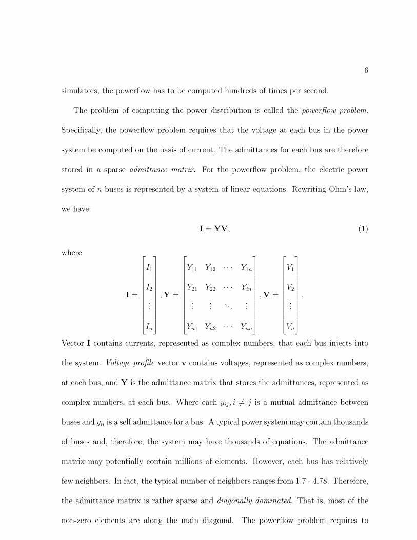
The problem of computing the power distribution is called the powerflow problem.
Specifically, the powerflow problem requires that the voltage at each bus in the power
system be computed on the basis of current. The admittances for each bus are therefore
stored in a sparse admittance matrix. For the powerflow problem, the electric power
system of n buses is represented by a system of linear equations. Rewriting Ohm’s law,
we have:
I = YV, (1)
where
I =
I1
I2
...
In
,Y =
Y11 Y12 · · · Y1n
Y21 Y22 · · · Yin
......
. . ....
Yn1 Yn2 · · · Ynn
,V =
V1
V2
...
Vn
.
Vector I contains currents, represented as complex numbers, that each bus injects into
the system. Voltage profile vector v contains voltages, represented as complex numbers,
at each bus, and Y is the admittance matrix that stores the admittances, represented as
complex numbers, at each bus. Where each yij, i 6= j is a mutual admittance between
buses and yii is a self admittance for a bus. A typical power system may contain thousands
of buses and, therefore, the system may have thousands of equations. The admittance
matrix may potentially contain millions of elements. However, each bus has relatively
few neighbors. In fact, the typical number of neighbors ranges from 1.7 - 4.78. Therefore,
the admittance matrix is rather sparse and diagonally dominated. That is, most of the
non-zero elements are along the main diagonal. The powerflow problem requires to

7
solve this system for voltages. One of the most straightforward methods is to invert the
admittance matrix and solve the system as follows: V = Y−1I. However, the processing
of the inverted matrix is rather computationally intensive. Even more problematic is
the matrix fill in. That is, even if the original matrix Y is sparse, its inverse is usually
dense. Using a dense multi-million element matrix to solve the powerflow problem is
prohibitively expensive both in storage and computation time.
One approach to overcome the fill in problem is factorization: rather than computing
the inverse, the factor matrices are calculated such that these factors preserve the sparsity
of the original matrix. For example, a well-known LU factorization technique converts
Y into two triangular factors Y = LU. The lower L and upper U triangular matrices
consist of zeros above and below the main diagonal respectively. Substituting the factors
in Formula 1 we get.
I = (LU)v (2)
Letting vector Uv = X, the system of linear equations in Formula 2 can be split into
two as follows:
I = LX,X = Uv. (3)
Since L is the lower triangular factor matrix, the first system of linear equations can
be solved for X by forward substitution. Then, since U is the upper triangular factor
matrix, the second system can be solved for v using backward substitution. Given that
U and L preserve the sparsity of the original admittance matrix, this method of solving
the linear system of equations results in substantial memory and computational resource
savings.

8
The computational demands for real-time power system state computation require
efficient powerflow computations. Such requirements are beyond the capabilities of even
the fastest modern day central processing units (CPU). One method of accelerating
power system state computation is through parallelization on multi-processor architec-
tures. However, the success in this direction has been limited thus far. One major
obstacle is that the powerflow computation, specifically solving I = YV is inherently
sequential. Nevertheless, such problems could become solvable when the number of par-
allel processors such as those on Graphical Processing Units (GPU) is large enough that
even minor concurrency gains result in significant performance improvements.
GPGPU. The GPU is a specialized processor used for image processing and 3D appli-
cations. In 1992, Silicon Graphics opened the programming interface to its hardware by
releasing the OpenGL library [5]. Spurred by the graphics and 3D gaming market, the
GPU has evolved into a massively parallel, many-core processor with significant compu-
tational power. In 2002, Mark Harris coined the term General-purpose computation on
graphics processing units (GPGPU) [6]. GPGPU uses a GPU to perform computations
that are not related to graphics processing. A main difference between the multi-core
CPU and the many-core GPU is that a many-core processor puts more cores in a given
thermal envelope than a multi-core processor does [7]. This makes many-core compu-
tation advantageous. The effect of a many-core system is that it does not suffer from
traditional problems that arise in multi-core systems, such as bus contention3. A typ-
ical GPU has hundreds of cores and is able to achieve high peak memory bandwidth
3In this sense, I mean a computer bus and not a power system bus

9
throughput. The GPU is designed for data-parallel computations. Data-parallel process-
ing on the GPU involves mapping data elements to parallel processing threads. That is,
each thread on the GPU performs the same instruction or program on a different piece of
data. Researchers and developers quickly realized the benefit of using GPUs to accelerate
data-parallel algorithms. GPUs are used in a variety of areas that include computational
biology and chemistry, the SETI project [8], protein folding, video accelerators, ray trac-
ing and more.
Several frameworks exist that allow the developer to write applications for the GPU
using several high level programming languages. OpenCL [9] is an example of one such
framework that allows developers to write applications that run on a variety of GPUs. Mi-
crosoft has contributed to the list of GPU frameworks by developing DirectCompute [10]
for DirectX. DirectCompute differs from OpenCL in that it utilizes DirectX and there-
fore is only for the Windows operating system. OpenCL can be run on all of the major
operating systems (Linux, Windows and OS X). There is a third solution available for
developers wishing to write GPU accelerated applications, named CUDA.
Compute Unified Device Architecture (CUDA) was introduced by NVIDIA in Novem-
ber 2006, and is a general purpose parallel computing architecture. Unlike OpenCL and
DirectCompute, CUDA only runs on NVIDIA GPUs. However, in most cases the tight
integration of hardware and software allows CUDA to achieve better performance results
than OpenCL and DirectCompute. The CUDA parallel programming model [11] con-
sists of an application that contains a sequential host program that may execute parallel
programs called kernels on the GPU. A kernel is the code that runs in parallel on the
GPU.

10
Related literature. Previous work has been done on sparse matrix vector (SpMV) mul-
tiplications using the GPU [12, 13, 14]. Bell et al. present several packing methods for
packing sparse matrices based on their storage requirements and computational charac-
teristics. Kernels are also included to illustrate generic SpMV multiplications. However,
the SpMV multiplication kernels presented would have to be heavily modified to solve
systems of linear equations using a bi-factorized matrix. Chalasani [15] presents several
approaches to computing the powerflow problem using parallelization. Chalasani’s work
differs from mine in that he is using a loosely coupled, heterogeneous network of worksta-
tions. The architecture of Chalasani’s work is incompatible with the GPU architecture
on which I will be implementing my algorithm. Furthermore, the use of a GPU is more
cost-effective than a cluster or workgroup of machines and will likely yield similar, if not
better, results. My implementation exploits the high level of parallelism offered by a
single GPU installed on a single workstation. Liu et al. [16] present a generic method for
SpMV multiplication using OpenMP. This implementation is limited by the number of
CPU cores on a given system. The alternative is to use OpenMP in on a cluster, how-
ever, this suffers from costly message passing. The generic SpMV multiplication method
is not suitable for SpMV solving systems of linear equations using a bi-factorized matrix.
Wang et al. [17] present a method for solving systems of linear equations using LU factor-
ization and a specialized FPGA multiprocessor. Their implementation requires several
compute nodes and several control nodes, which may lead to cumbersome and complex
configurations. This approach differs from my setup in that I use one machine with one
GPU, which is incompatible with the requirements of Wang’s work. Amestoy et al. [18]

11
present a multifrontal parallel distributed solver that utilizes a MIMD architecture to
factorize dense and sparse matrices to solve systems of linear equations. Their approach
requires a host node to analyze the matrix, break up the work, distribute the work, col-
lect the solution and organize the compute nodes during the computation process. In my
approach, the hardware schedulers on the GPU distribute work to the multiprocessors
on the same GPU and the multiprocessors utilize their local resources to complete the
computations, thus not relying on the hardware schedulers, or a single host node for fur-
ther instructions. Furthermore, in my implementation, the mapping of data to a group
of threads is intuitively based on the thread ID and requires no analysis of the incom-
ing sparse matrix4. Arnold et al. [19] present an elemental scheme for distributing the
LU factor matrices across a MIMD processor. The elemental scheme analyzes all of the
tasks to find tasks “ready” to be processed and assigns them to an idle processor. The
management overhead for this method could lead to significant compromises in efficiency
when the matrix is significantly sparse. My method packs the sparse matrix in a format
that ignores all non-zero elements, such that analyzing the matrix for “ready” tasks is
not necessary.
Several linear algebra libraries have also been developed to aide in the process of
solving linear equations using the GPU, such as CUBLAS [20] and CUSP [21]. These
libraries, however, are for generic matrix vector computations, and are not suitable for
my purposes. Mayanglambam et al. [22] implements a library, TAUCUDA, for CUDA
developers to accurately test the complete performance of their parallel applications.
Their library takes into account asynchronous and synchronous operations. The setup of
4I assume the incoming matrix has already been sorted by row

12
my kernels is straightforward and allows for performance measurements to be computed
without the use of additional libraries. To my knowledge, this is the first time that a
GPU is used to solve systems of linear equations using factorized, specifically bi-factorized
matrices.
Thesis outline. In this thesis I explore the performance improvement of the powerflow
computation by parallelizing the least parallelizable component of the powerflow problem:
the sparse linear equation solver. In Chapter 2, I explain the bi-factorization method
that factorizes a matrix into two factor matrices, while preserving the sparsity of the
original admittance matrix. I also explain how to solve systems of linear equations
using bi-factorized matrices. In Chapter 2, I also explain what CUDA is and how it
can be used to accelerate the powerflow computation. I then present a parallel sparse
linear equation solver for bi-factorized matrices. I implement this algorithm using a cost-
effective commodity NVIDIA GPU. I build a system to accurately produce sample power
system data. I also discuss the optimization process. In Chapter 3, I explain the setup
of my hardware and software used for the test environment. I also explain the process
of generating the data that is used in our performance tests. In Chapter 4, I present the
results from my experiments show that my approach achieves up to a 38 times speedup
over a single threaded CPU implementation. In Chapter 5, I present my plans for future
work.

CHAPTER 2
Preliminaries
To implement a high performance parallel sparse linear equation solver, I created a
random power system topology generator. The random power system topology generator
produces realistic sample admittance matrices. To solve a system for voltages, the ad-
mittance matrix is factorized using bi-factorization. I explain how CUDA and the GPU
can be used to parallelize the sparse linear equation solver.
2.1 Bi-factorization
Bi-factorization is particularly suitable for sparse coefficient matrices that are diago-
nally dominant and that are either symmetrical, or, if not symmetrical, have a symmet-
rical sparsity structure [23]. Electric networks and power flow systems adhere to these
requirements. A factorization approach is to separate the matrix into multiple factor
matrices. This method is based on finding 2n factor matrices, such that the product of
these factor matrices satisfies the requirement:
L(n)L(n−1) . . .L(2)L(1)YU(1)U(2) . . .U(n−1)U(n) = E (4)
where
Y = original coefficient matrix,
L = lower factor matrices,
U = upper factor matrices,
13
14
E = unit matrix of order n.
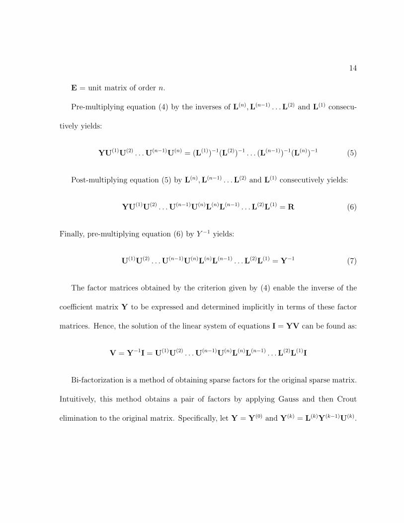
Pre-multiplying equation (4) by the inverses of L(n),L(n−1) . . .L(2) and L(1) consecu-
tively yields:
YU(1)U(2) . . .U(n−1)U(n) = (L(1))−1(L(2))−1 . . . (L(n−1))−1(L(n))−1 (5)
Post-multiplying equation (5) by L(n),L(n−1) . . .L(2) and L(1) consecutively yields:
YU(1)U(2) . . .U(n−1)U(n)L(n)L(n−1) . . .L(2)L(1) = R (6)
Finally, pre-multiplying equation (6) by Y −1 yields:
U(1)U(2) . . .U(n−1)U(n)L(n)L(n−1) . . .L(2)L(1) = Y−1 (7)
The factor matrices obtained by the criterion given by (4) enable the inverse of the
coefficient matrix Y to be expressed and determined implicitly in terms of these factor
matrices. Hence, the solution of the linear system of equations I = YV can be found as:
V = Y−1I = U(1)U(2) . . .U(n−1)U(n)L(n)L(n−1) . . .L(2)L(1)I
Bi-factorization is a method of obtaining sparse factors for the original sparse matrix.
Intuitively, this method obtains a pair of factors by applying Gauss and then Crout
elimination to the original matrix. Specifically, let Y = Y(0) and Y(k) = L(k)Y(k−1)U(k).

15
Where
L(k) =
1 0
. . ....
1 0
l(k)kk
l(k)ik 1
.... . .
l(k)nk 1
,
U(k) =
1
. . .
1
0 · · · 0 1 u(k)kj · · · u
(k)kn
1
. . .
1
,
Y(k) =
1 0
. . ....
1
y(k)kk y
(k)kj · · · y
(k)kn
0 · · · y(k)ik y
(k)ij y
(k)in
.... . .
...
y(k)nk · · · y
(k)nn
.

16
The elements of these matrices are as follows:
l(k)ik = −y
(k−1)ik
y(k−1)kk
(i = k + 1, . . . , n),
u(k)kj = −
y(k−1)kj
y(k−1)kk
(j = k + 1, . . . , n),
y(k)ij = y
(k−1)ij −
y(k−1)ik y
(k−1)ij
y(k−1)kk
(i = k + 1, . . . , n)
(j = k + 1, . . . , n)
.
Note that if y(k−1)ik is zero, so is l
(k)ik . Similarly, if l
(k−1)kj is zero, so is u
(k)kj . That is, sparse
Y(k−1) produces sparse factors L(k) and U(k). These factor matrices are conveniently
stored compactly as a collection of factor matrices in one large matrix. As such, there is
a certain amount of fill in with regard to the entire matrix as we transition from Y(k−1)
to Y(k), but it tends to be insignificant. This fill in is further minimized if the rows
and columns in Y are sorted in the increasing order of the number of non-zero elements.
Thus, if Y is sparse, the 2n factors produced by bi-factorization are also sparse. Note
also that in every factor L(k) and U(k), only the respective column and row above and
below the diagonal is non-zero. Therefore, all the 2n factors can be compactly stored as
rows and columns in a single factorized n× n matrix.
2.2 CUDA Overview
GPU architecture. The newest generation of GPUs by NVIDIA, code named Fermi,
feature up to 512 CUDA cores. A CUDA core is a streaming processor on the GPU.
Each CUDA core features a fully pipelined integer arithmetic logic unit and a floating
point unit1. The architecture was designed with double precision arithmetic in mind,
1The Fermi architecture implements the new IEEE 754-2008 floating point standard.

17
offering up to 16 double precision fused multiply-add operations per SM, per clock tick.
The core executes one floating point or integer instruction per clock tick per core. The
CUDA cores are organized into 16 streaming multiprocessors (SM) of 32 cores each. A
streaming multiprocessor is a grouping of 32 CUDA cores, all of which have access to 16
load/store units, 4 special function units, an interconnection network, 64KB of shared
memory and 32,768 registers. A thread is an independent execution stream that runs a
piece of the code based on the data to which it is assigned. A core may execute many
threads, but may only execute one thread at a time. A thread block is a logical grouping
of threads that guarantees that all threads within a thread block reside on the same
SM. The threads within a given thread block cooperate and communicate using barrier
synchronization. Each thread block operates independently of all other thread blocks.
The GigaThread global scheduler distributes thread blocks to SM thread schedulers as
efficiently as possible. It is important to note that in order to achieve the highest level
of efficiency, the GigaThread global scheduler distributes work to the thread blocks in
an arbitrary order. That is, one can not assume that thread block zero will be executed
before thread block one and so on. The GPU has a 384-bit memory interface, which
allows up to a total of 6 GB of GDDR5 DRAM memory.
CUDA threads have access to multiple types of memory during their execution. See
Figure 2 for illustration2. Each thread has private local, register based memory, which
is fast but quite small. Each thread block has access to slower shared memory, which is
accessible to all threads of the local thread block. Shared memory is located at each SM
and is limited to 64 KB. The scope of the data in shared memory is the local thread block.
2This figure was taken from NVIDIA’s CUDA Programming Guide [11].

18
Threads of all thread blocks have access to the large global memory. Global memory is
the DRAM located off-chip on the GPU. The access to the global memory is significantly
slower than access to the on-chip memory. Therefore, the usage of global memory should
be minimized.
Software. A CUDA program consists of two essential components: the host code and
the kernel code. Host code is the code that runs on the CPU. Host code is responsible
for calling the parallel kernels. Kernel code is the code that runs in parallel on the GPU.
A kernel is a Single Program Multiple Data (SPMD) code that is executed on the GPU
using a potentially large number of parallel threads. Multiple GPU threads run the
kernel. Each thread has a unique thread ID. A programmer can refer to an individual
thread by its thread ID. The thread ID is a three-dimensional vector. The programmer
or compiler organizes threads into thread blocks. In the Fermi architecture, each thread
block may contain up to 1,024 threads, with a maximum of 65,535 thread blocks. This
means that a programmer has a total of over 67 million threads at his or her disposal,
which provides a high degree of potential parallelism.

19
Figure 2: CUDA memory hierarchy.

20
2.3 Random Power System Generator
Before I can test the performance of my parallel algorithm, I need to generate random
admittance matrices to model realistic power systems. The standard practice for engi-
neering applications is to use a small number of historical test systems. This practice,
however, has shortcomings when examining new theories, methods and scalability. In my
system, I develop a random power system topology generator that generates statistically
accurate, realistic power system topologies.
Studies of power systems in the United States indicate that the average number of
neighbors is about 2.67 for Western Electricity Coordinating Council system (WECC),
formerly known as the Western Systems Coordinating Council, and about 4.78 for the
New York Independent System Operator (NYISO) system [24]. The Siberian region of the
Unified Power System of the Russian Federation (UPS) has 1.7 neighbors on average [25].
A random power system topology is generated using a random distribution function.
The generated power system topology has no self-loops and no disconnected nodes. Inside
a fixed square, N bus locations are selected using a random distribution function. The
edges, which represent transmission lines, are chosen according to the distance limitation
dmin ≤ d ≤ dmax. Each bus is assigned a corresponding random Poisson variable, P (λ),
that represents the potential number of neighbors. λ is equal to the average number
of neighbors for each bus in the power system. A potential list of neighbors, X, is
calculated using the distance limitation and the random Poisson variable for each bus.
It is important to note that in some cases X < P (λ). In such cases, the number of X
neighbors is chosen over P (λ). The output of the random power system is the admittance

21
matrix Y. Matrix Y is stored in Coordinate List (COO) format. An example of COO is
given in Figure 3. See Figures 4 - 7 for examples of generated power system topologies
A =
0 2 + j1.2 0 0
0 0 4− j2.1 1 + j0.9
12 + j6.7 0 0 0
0 0 0 4 + j2.3
value row column
2 + j1.2 0 1
4− j2.1 1 2
1 + j0.9 1 3
12 + j6.7 2 0
4 + j2.3 3 3
Figure 3: A COO representation of sample matrix A

22
0
0.2
0.4
0.6
0.8
1
0 0.2 0.4 0.6 0.8 1
Figure 4: A 20 node random power system topology: dmin=0, dmax=0.3, λ = 2.67.
0
0.2
0.4
0.6
0.8
1
0 0.2 0.4 0.6 0.8 1
Figure 5: A 20 node random power system topology: dmin=0, dmax=0.3, λ = 4.78.

23
0
0.2
0.4
0.6
0.8
1
0 0.2 0.4 0.6 0.8 1
Figure 6: A 100 node random power system topology: dmin=0, dmax=0.3, λ = 2.67.
0
0.2
0.4
0.6
0.8
1
0 0.2 0.4 0.6 0.8 1
Figure 7: A 100 node random power system topology: dmin=0, dmax=0.3, λ = 4.78.

24
2.4 Parallel Sparse Linear Equation Solver
Even though solving systems of linear equations with bi-factorized matrices is inher-
ently sequential, I have identified portions of calculations on the sparse matrix that can be
performed concurrently. In my method, I pack all non-zero elements of the bi-factorized
matrix into COO format.
Development history. It took me several attempts to optimize the algorithm. I started
out with a non-packed N ×N admittance matrix and a kernel that consisted of as many
threads as possible inside of one block. The algorithm used the CPU to control its
execution sequentially. As such, my first attempt actually did worse than the CPU.
Next, I took a look at the data and figured out that the COO format would work well for
my purposes. The algorithm was then rewritten to handle the new format. As such, I
reconfigured the kernel launch parameters such that the kernels had one thread per matrix
element. This involved having many blocks with many threads. CUDA executes blocks
in an arbitrary order, therefore the programmer does not have control over the thread
block execution. The data dependencies of the algorithm require that while multiplying
factor matrix L by voltage vector v, column k must finish processing before column
k+ 1 may begin. Similarly, for factor matrix U, row k must finish processing before row
k − 1 may be begin. Since I was using many blocks, I had to use the CPU to launch
the kernel sequentially to avoid data-dependency violations. Upon running NVIDIA’s
CUDA Profiler, I discovered that over 80% of the execution time was spent calling the
kernels sequentially. In fact, even with a packed sparse matrix, the GPU algorithm

25
was still achieving only a 2-4 times speedup over the CPU. Therefore, I decided that
having one thread block with a couple hundred threads would be better. That is, I could
launch the kernels one time, and have them loop through the matrix without needing to
coordinate with the CPU. Once I implemented this method, I started observing a 10-18
times speedup. After reviewing the requirements of the algorithm, as well as reviewing
the data dependencies, I identified several areas where I could utilize shared memory.
Utilization of shared memory led to a 22-27 times speedup.
My final optimization came after discovering that the GPU and my algorithm had
troubles processing the data when Y had more than 1, 000, 000 non-zero elements. When
the number of non-zeros in the admittance matrix exceeds 1, 000, 000, the solution vector
is returned with zeros. I believe it has to do with a memory overflow, but I have not
determined the exact cause. Previously, I used atomic operations to keep track of how
many non-zero elements were in a given row or column. Keeping track of this number
allowed the kernels to increment a position counter in order to move from column to
column or row to row. Instead, I created an array to keep track of how many elements
are in a given row or column. I send the array of row and column position values to the
GPU and increment the position counter accordingly. This final optimization increased
the speedup to 38 times over the CPU.
The process of learning to program on the GPU was not without trial and error.
Several behaviors of the GPU are not well documented within the CUDA documentation.
For instance, during testing, I found that my algorithm would produce incorrect results
when testing against admittance matrices in a specific order. When I ran the admittance
matrices in a different order, the results would be correct. This discrepancy was due to a

26
memory initialization issue. I assumed that when I freed the memory, it and its contents
were gone. Furthermore, I assumed that when I allocated new memory and initialized it
in the next run of the application, the memory would be properly initialized. However, I
found that I had to not only initialize the memory before I used it, but I had to reinitialize
the memory before freeing it and exiting.
L kernel. Since the data dependencies for processing Lv only require that column k
be processed before column k + 1, all of the elements in column k on or below the main
diagonal are able to be processed in parallel. To calculate the values of v′j, threads are
mapped to all elements of the kth column of L where i = k and j ≥ i. The values of v′j are
calculated such that v′j = vj+ljiviwhere i < j < n, and v′i = liivi where i = k and j = k.
U kernel. The data dependencies for processing UV require that row k be processed
before row k − 1. Furthermore, for row k the sum of uijvj must be computed where
i = k and j > k. The product of uijvj can be computed in parallel. Using strategies
from [26, 27], I implement a parallel reduction function to compute the sum of uijvj
efficiently in parallel.
Parallel reduction. The parallel reduction code uses N/2 active threads, where N is
the number of threads in the block, to compute the sum of uijvj. That is, thread 0 and
thread N−1 compute their sum, thread 1 and thread N−2 compute their sum, thread n
and thread N − (n+ 1) compute their sum and so on. Each iteration of the for loop cuts
the number of active threads in half while storing the partial sums in shared memory

27
mapped to the lower half of the active threads. Normally, a parallel reduction on the GPU
makes use of multiple thread blocks to sum very large arrays in parallel. In this case,
however, there is only one block available, as the reduction code is implemented inside
of the U kernel code. However, the array is not large and never exceeds the number of
threads in the thread block. My method is as efficient as a many-block implementation,
as it is only necessary to sum an array of size N . Furthermore, there is no need to sum
the partial sums for each thread block at the end. To further speed up this reduction,
the product of uijvj is stored in shared memory, and thus there is no need to load shared
memory from global for the reduction.
Number of Buses L kernel, ms U kernel with reduction, ms
500 0.99 2.46
1000 1.98 4.94
2000 4.00 9.91
3000 6.01 14.87
4000 8.13 19.85
5000 10.31 24.86
6000 12.36 29.83
7000 14.75 34.89
8000 16.84 39.88
9000 19.24 44.95
Table 1: Average computation times for L and U when average neighbor count is 2.67.
Table 1 displays the timings for the L kernel and the U kernel with the reduction code.

28
The U kernel time is generally double that of the L kernel, as the U timing contains the
code to perform a parallel reduction.

CHAPTER 3
Experiment Setup
Hardware. The test environment I used to evaluate the performance of the GPU versus
the CPU is a PC with an Intel i7 processor running at 2.8 GHz, 8 GB of DDR3 RAM
and an NVIDIA GTX 570. The GTX 570 has an over clocked processor clock running at
1.9 GHz and a memory clock running at 2.3 GHz. The GTX 570 has 480 CUDA cores
and a 320-bit memory interface with 1.28 GB of GDDR5 DRAM. It is also important to
note that the GTX 570 is not a dedicated GPU, and has to deal with both CUDA and
GUI programs.
Software. The host OS is Windows 7 64-bit Enterprise Edition. I wrote the CPU
algorithm using C# and compiled it with Visual Studio 2008, version 9.0, with .NET
framework 3.5 SP1. The CPU algorithm is not optimized and is single threaded. I wrote
the GPU algorithm using the CUDA toolkit v3.2 in C and compiled it using NVIDIA’s
nvcc compiler from within Visual Studio 2008.
Data generation. I selected the following system sizes for the UPS and WECC systems:
500, 1000, 2000, 3000, 4000, 5000, 6000, 7000, 8000 and 9000. For the NYISO system,
the system size was limited to 6000, as system sizes of 7000 and greater contained more
than 1, 000, 000 non-zero elements. For each system size, I generated 30 matrices. See
29

30
Tables 2 - 4 and Figures 8 - 10 for the average numbers of non-zero elements per sample
size and their densities. These matrices were generated off line before the performance
testing began. The confidence intervals shown in the graphs were calculated using a
t-distribution function where α was set to 99%.
The fill in appears large, however, Table 2 shows that the sparsity still remains.
Number of Buses Original Factorized Fill in Density, %
500 1030.6± 0.99 1399.6± 136.41 369 0.56
1000 2078.6± 2.18 3468± 417.00 1389.4 0.35
2000 3919.06± 0.99 7807.2± 992.79 3888.14 0.20
3000 6254± 1.94 13981± 3669.27 7727 0.16
4000 8297.2± 1.44 23738.4± 4558.57 15441.2 0.15
5000 10386± 2.56 35419.4± 5719.57 25033.4 0.14
6000 12432± 2.17 41171.4± 9113.15 28739.4 0.11
7000 14457± 2.00 53392.6± 13778.59 38935.6 0.11
8000 16572.4± 2.71 76363.8± 19466.18 59791.4 0.12
9000 18609.2± 1.99 89030.2± 18239.76 70421 0.11
Table 2: Average number of elements in the admittance matrix for UPS.

31
0
20000
40000
60000
80000
100000
120000
500 1000 2000 3000 4000 5000 6000 7000 8000 9000
Mat
rix S
ize
Number of Buses
Average Admittance Matrix Size for Siberian UPS
OriginalFactorized
Figure 8: Average admittance matrix size with λ = 1.7.
32
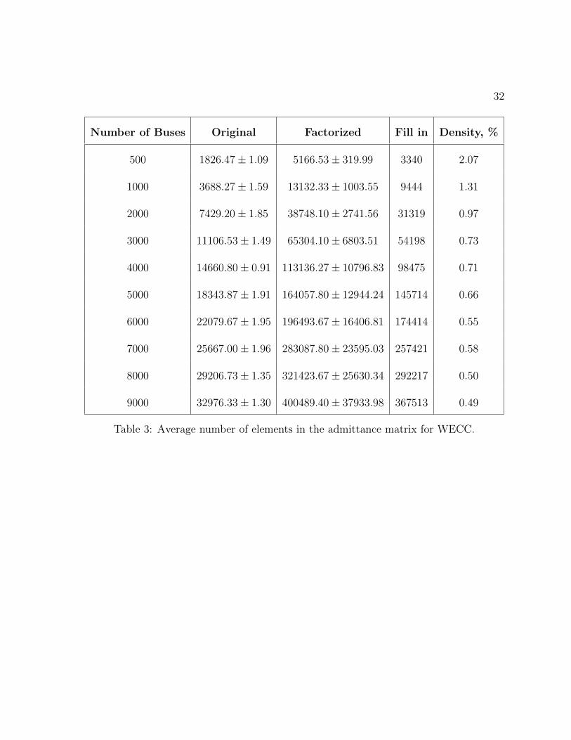
Number of Buses Original Factorized Fill in Density, %
500 1826.47± 1.09 5166.53± 319.99 3340 2.07
1000 3688.27± 1.59 13132.33± 1003.55 9444 1.31
2000 7429.20± 1.85 38748.10± 2741.56 31319 0.97
3000 11106.53± 1.49 65304.10± 6803.51 54198 0.73
4000 14660.80± 0.91 113136.27± 10796.83 98475 0.71
5000 18343.87± 1.91 164057.80± 12944.24 145714 0.66
6000 22079.67± 1.95 196493.67± 16406.81 174414 0.55
7000 25667.00± 1.96 283087.80± 23595.03 257421 0.58
8000 29206.73± 1.35 321423.67± 25630.34 292217 0.50
9000 32976.33± 1.30 400489.40± 37933.98 367513 0.49
Table 3: Average number of elements in the admittance matrix for WECC.
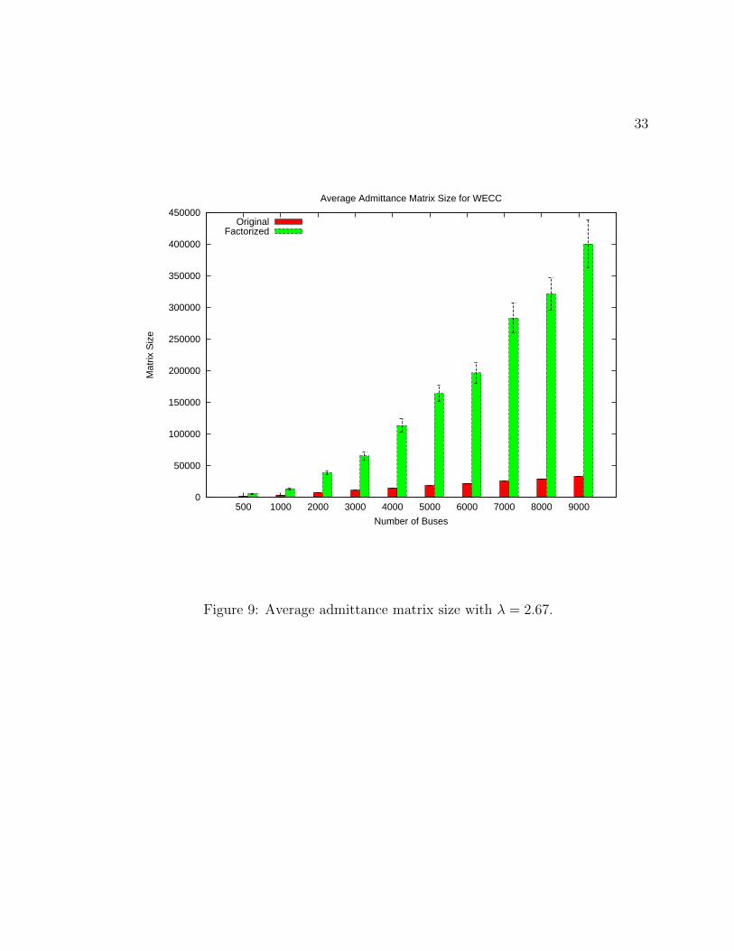
33
0
50000
100000
150000
200000
250000
300000
350000
400000
450000
500 1000 2000 3000 4000 5000 6000 7000 8000 9000
Mat
rix S
ize
Number of Buses
Average Admittance Matrix Size for WECC
OriginalFactorized
Figure 9: Average admittance matrix size with λ = 2.67.

34
Number of Buses Original Factorized Fill in Density, %
500 2863.6± 3.22 15085.4± 1895.54 12222 6.03
1000 5760± 5.52 39518.2± 5933.89 33758 3.95
2000 11489.8± 7.52 39518.2± 16387.82 91739 2.58
3000 17163.4± 6.07 103228.4± 19112.85 161712 1.99
4000 22899.6± 6.74 365619± 48518.50 342719 2.29
5000 28594.2± 5.70 498994.2± 116629.32 470400 2.00
6000 34166.4± 4.76 609192.4± 145238.24 575026 1.69
Table 4: Average number of elements in the admittance matrix for NYISO.

35
0
20000
40000
60000
80000
100000
120000
500 1000 2000 3000 4000 5000 6000 7000 8000 9000
Mat
rix S
ize
Number of Buses
Average Admittance Matrix Size for NYISO
OriginalFactorized
Figure 10: Average admittance matrix size with λ = 4.78.
For the reader’s consideration, I have included Tables 5 - 7, which show the average
data transfer times for the admittance matrices to and from the GPU.

36
Number of Buses To Card, ms From Card, ms
500 0.22 0.13
1000 0.28 0.11
2000 0.49 0.13
3000 0.59 0.14
4000 0.87 0.17
5000 1.21 0.18
6000 1.42 0.19
7000 1.81 0.21
8000 2.29 0.22
9000 2.54 0.24
Table 5: Average memory transfer times for λ = 1.7.

37
Number of Buses To Card, ms From Card, ms
500 0.29 0.09
1000 0.51 0.10
2000 1.16 0.12
3000 1.84 0.15
4000 2.85 0.15
5000 3.88 0.16
6000 4.63 0.19
7000 6.19 0.20
8000 7.04 0.21
9000 8.77 0.24
Table 6: Average memory transfer times for λ = 2.67.
Number of Buses To Card, ms From Card, ms
500 0.55 0.10
1000 1.17 0.11
2000 2.60 0.13
3000 4.29 0.14
4000 7.90 0.16
5000 10.71 0.17
6000 12.98 0.24
Table 7: Average memory transfer times for λ = 4.78.

38
In order to assess the efficiency of my algorithm, I collected performance data using
the previously generated matrices. For each generated matrix I measured the time that it
takes to execute the algorithm on the CPU and the GPU. For each run of the programs,
a third program is run that checks the CPU and GPU output for correctness.
In the case of C#, the resolution of the default timer, stopwatch(), was not suffi-
ciently high. In fact, I observed that the default C# timer is only accurate up to about
15 ms. Using methods in [28], I developed a high-precision timer, accurate to 1 ns.
CUDA comes with a high resolution event timer API [29]. The event timer creates
a GPU event, destroys the event and records the duration using a time stamp, which is
later converted to a floating-point value representing milliseconds.

CHAPTER 4
Experiment Results and Analysis
Since my goal is to measure the performance of CUDA kernels, I do not include the
time spent transferring data between host and GPU in the average computation time
table. Although I developed a system to produce realistic power system topologies, it is
important to note that the uniformly distributed random values that were generated for
admittances and voltages may not be indicative enough to test the performance of my
algorithm. In the future I would like to compare the following results against realistic
values. Figures 11 - 13 show the average computation time in milliseconds for all sample
sizes for the CPU and the GPU. Since my sample sizes only contained 30 matrices, I have
included confidence intervals on the graphs. The confidence intervals were calculated
using a t-distribution function where α was set to 99%.
39

40
0
500
1000
1500
2000
2500
500 1000 2000 3000 4000 5000 6000 7000 8000 9000
Tim
e, m
s
Number of Buses
Average Computation Time for Siberian Region of Russian UPS
GPUCPU
Figure 11: Average computation time for CPU versus GPU with λ = 1.7.

41
Number of Buses GPU, ms CPU, ms Speedup
500 3.34± 0.00 6.53± 0.18 1.96
1000 6.68± 0.01 22.33± 0.49 3.34
2000 13.35± 0.01 89.88± 4.11 6.73
3000 20.07± 0.06 204.88± 4.69 10.21
4000 26.82± 0.04 377.22± 4.15 14.06
5000 33.56± 0.05 597.67± 9.46 17.81
6000 40.25± 0.07 1010.93± 7.32 25.12
7000 47.07± 0.10 1301.54± 15.71 27.65
8000 53.89± 0.11 2099.35± 17.41 38.96
9000 60.66± 0.09 2327.66± 26.77 38.37
Table 8: Average computation times with λ = 1.7.
Table 8 has the average computation times for CPU versus GPU with the average
speedup for each sample size for the UPS system.

42
0
500
1000
1500
2000
2500
500 1000 2000 3000 4000 5000 6000 7000 8000 9000
Tim
e, m
s
Number of Buses
Average Computation Time for WECC
GPUCPU
Figure 12: Average computation time for CPU versus GPU with λ = 2.67.

43
Number of Buses GPU, ms CPU, ms Speedup
500 3.45± 0.01 6.76± 0.07 1.96
1000 6.92± 0.01 23.08± 0.31 3.34
2000 13.91± 0.02 97.21± 1.04 6.99
3000 20.88± 0.06 224.19± 4.41 10.74
4000 27.99± 0.1 408.62± 3.47 14.60
5000 35.16± 0.13 643.11± 15.51 18.29
6000 42.19± 0.16 1048.77± 8.94 24.85
7000 49.65± 0.24 1364.36± 9.26 27.49
8000 56.72± 0.24 2105.36± 7.75 37.12
9000 64.19± 0.36 2385.62± 22.93 37.16
Table 9: Average computation times with λ = 2.67.
Table 9 has the average computation times for CPU versus GPU with the average
speedup for each sample size for WECC.

44
0
200
400
600
800
1000
1200
500 1000 2000 3000 4000 5000 6000
Tim
e, m
s
Number of Buses
Average Computation Time for NYISO
GPUCPU
Figure 13: Average computation time for CPU versus GPU with λ = 4.78.

45
Number of Buses GPU, ms CPU, ms Speedup
500 3.58± 0.02 6.97± 0.32 1.95
1000 7.21± 0.05 25.26± 0.73 3.50
2000 14.54± 0.15 100.84± 5.58 6.94
3000 21.98± 0.18 235..77± 13.66 10.73
4000 30.21± 0.49 425.92± 17.71 14.10
5000 38.13± 1.22 667.84± 16.16 17.51
6000 45.88± 1.58 1113.95± 30.43 24.86
Table 10: Average computation times with λ = 4.78.
Table 10 has the average computation times for CPU versus GPU with the average
speedup for each sample size for NYISO.
My results show that the use of a GPU for solving sparse linear equations with
bi-factorized matrices achieves up to a 38 times speedup over the traditional CPU im-
plementation. This result highlights the practical use of a GPU for a high performance
sparse linear equation solver. My kernels identify and exploit parallelism in an otherwise
sequential algorithm.
CHAPTER 5
Future Work
Future work. I plan to further optimize the kernels with the goal of being able to
compute matrices with more than 1,000,000 non-zero elements. The next revision of the
code will have a strong focus on memory access optimization on the GPU. The current
implementation receives the admittance matrix pre-sorted by row, the algorithm makes
a copy and sorts the matrix by column using the CPU. I plan to explore two options for
addressing these sorting issues. First, I plan to implement an efficient parallel sorter to
sort the matrix in place on the GPU. Second, I plan to explore a method where the matrix
does not require prior sorting. I also plan to optimize my parallel reduction code further,
such that only non-zero elements are processed. I plan to implement additional parts of
the powerflow computation where the GPU could be used to accelerate the computation
further. In order for this software to be adapted into industrial use, the sorting issues
will have to be resolved.
46

APPENDIX A
CUDA Solver Source Code
#include <stdio.h>
#include <stdlib.h>
#include <time.h>
#include "cuda.h"
#define nTL 1024 // num threads for L kernel
#define nTU 1024 // num threads for U kernel
typedef struct
{
double x, y; // x = real, y = imaginary
int px, py; // px = position x, py = position y
}cuDoubleComplex;
void writeVector(cuDoubleComplex *v, FILE* f,int N);
void importMatrix(FILE *f, cuDoubleComplex *m, cuDoubleComplex *m2,
int *countersx, int *countersy);
void importVector(FILE *f, cuDoubleComplex *m);
int countVector(FILE *f);
int int_cmp(const void *A, const void *B);
// OPERATOR OVERLOADS
__device__ __forceinline__ cuDoubleComplex operator*(const cuDoubleComplex a,
const cuDoubleComplex b){
cuDoubleComplex result;
result.x = (a.x * b.x) - (a.y * b.y);
result.y = (a.y * b.x) + (a.x * b.y);
return result;
}
__device__ __forceinline__ cuDoubleComplex operator+(const cuDoubleComplex a,
const cuDoubleComplex b){
cuDoubleComplex result;
result.x = (a.x + b.x);
result.y = (a.y + b.y);
return result;
}
__device__ __forceinline__ cuDoubleComplex operator-(const cuDoubleComplex a,
const cuDoubleComplex b){
cuDoubleComplex result;
result.x = a.x - b.x;
result.y = a.y - b.y;
return result;
47

48
}
__device__ __forceinline__ cuDoubleComplex operator/(const cuDoubleComplex a,
const cuDoubleComplex b){
cuDoubleComplex result;
result.x = (((a.x * b.x) + (a.y * b.y)) / ((pow(b.x, 2)) + (pow(b.y, 2))));
result.y = (((a.y * b.x) - (a.x * b.y) ) / ((pow(b.x, 2)) + (pow(b.y, 2))));
return result;
}
// END OPERATOR OVERLOADING
// boolean value to determine if a block is the last block done or not
__shared__ bool isLastBlockDone;
__global__ void L(cuDoubleComplex *a, cuDoubleComplex* b,
cuDoubleComplex *c, int N, int ne, int *count,
unsigned int *index){
// variable to keep track of how many elements match the current col, num
__shared__ unsigned int placeholder;
if(threadIdx.x==0)
placeholder=0; // start at 0
__syncthreads();
for(int i = 0; i < N; i++){
int tid = placeholder + threadIdx.x;
// extract row, col coordinates from COO format
// and assign them to x and y for each thread
int x = a[tid].px; int y = a[tid].py;
if(x == i && y == i){
// hardcode special case where num==0
if(i==0){
// number on the diagonal for num=0 v’_i = l_ii * v_i
c[i] = a[i] * b[i];
}else{
// number on the diagonal v’_i = l_ii * v_i
c[i] = a[tid] * b[i];
}
}
__syncthreads();
if(x == i && y > i){
// v’_j = v_j + l_ji * v_i
b[y] = b[y] + a[tid] * b[i];
}
// increment tid by placeholder
if(threadIdx.x==0) placeholder += count[i];
__syncthreads();
}
}

49
__global__ void U(cuDoubleComplex *a, cuDoubleComplex* b,
cuDoubleComplex *c, int N, int ne, int *count,
unsigned int *index){
// start kernel at end of matrix and work our way up
int tid = ne - threadIdx.x;
int t = threadIdx.x;
// variable to keep track of how many elements match the current col, num
__shared__ unsigned int placeholder;
if(threadIdx.x==0) placeholder = 0;
__syncthreads();
for(int num = N-1; num >=0; num--){
// decrement tid by number of elements minus placeholder
tid = (ne-placeholder) - t;
// extract row, col coordinates from COO format and
// assign them to x and y for each thread
int x = a[tid].px; int y = a[tid].py;
// setup shared memory array of size nTU for faster access
__shared__ cuDoubleComplex sdata[nTU];
// initialize shared memory to 0
sdata[t].x=0;sdata[t].y=0;
if(y == num && x > num){
// u_ji * v_j
sdata[t] = a[tid] * c[x];
}
__syncthreads();
// begin parallel reduction
// cut number of active threads in half for each iteration
for(unsigned int s=blockDim.x/2; s>0; s>>=1)
{
if (t < s){
// add lower threads to higher threads and store results in
// lower threads. sum(u_ji * v_j)
sdata[t] = sdata[t] + sdata[t + s];
}
__syncthreads();
}
// write results to global memory
if(t==0){
c[num] = c[num] + sdata[0];
// increment placeholder counter
placeholder += count[num];
}
__syncthreads();
}

50
}
int main(int argc, char *argv[]){
/**************************************
call functions to:
import matrix and vector
launch parallel kernels
record results in a file
**************************************/
// variables for reading powerflow data based on command line arguments
char Ystring[50], Vin[50];
sprintf(Ystring, "PGen/Y_%d_%d.csv", atoi(argv[1]), atoi(argv[2]));
sprintf(Vin, "PGen/V_%d_%d.csv", atoi(argv[1]), atoi(argv[2]));
FILE *cout = fopen("IO/cudaB.csv", "w");
FILE *cout2 = fopen("IO/cudaB2.csv", "w");
FILE *results = fopen("IO/results.csv", "a");
FILE *Y = fopen(Ystring,"r");
FILE *V = fopen(Vin,"r");
// ne = number of elements, ctr for keeping track of kernel calls
int ne;
// size of matrix N*N
const int N = atoi(argv[1]);
// cuda event timers - two timers per event, start and stop
cudaEvent_t lCompute, lComputeS, d2gMem, d2gMemS, g2dMem, g2dMemS,
uCompute, uComputeS;
// cuda event timer totals
float lComputeT, d2gMemT, g2dMemT, uComputeT;
// count number of elements in the packed matrix
ne = countVector(Y);
// close file to reset the fh
fclose(Y);
// reopen the matrix file and actually import it
FILE *Yin = fopen(Ystring,"r");
// setup matrix A and allocate host mem
unsigned int size_a = ne;
unsigned int mem_size_a = sizeof(cuDoubleComplex) * size_a;
// setup arrays B, C and allocate host mem
unsigned int size_b = N;
unsigned int mem_size_b = sizeof(cuDoubleComplex) * size_b;
unsigned int size_c = N;
unsigned int mem_size_c = sizeof(cuDoubleComplex) * size_c;
// allocate memory for matrix and arrays
// col sorted matrix

51
cuDoubleComplex* a = (cuDoubleComplex*)malloc(mem_size_a);
// row sorted matrix
cuDoubleComplex* a1= (cuDoubleComplex*)malloc(mem_size_a);
// dense voltage vector
cuDoubleComplex* b = (cuDoubleComplex*)malloc(mem_size_b);
// results vector
cuDoubleComplex* c = (cuDoubleComplex*)malloc(mem_size_c);
// array to store num elements for each column
int *countersx = (int*)malloc(sizeof(int)*N);
// array to store num elements for each row
int *countersy = (int*)malloc(sizeof(int)*N);
// initialize elements to 0
memset(countersx, 0, sizeof(int)*N);
memset(countersy, 0, sizeof(int)*N);
// debugging variable to keep track of num elements processed
unsigned int *h_index = (unsigned int*)malloc(
sizeof(unsigned int));
// import the randomly generated admittance matrix
importMatrix(Yin, a, a1, countersx, countersy);
// import the randomly generated voltage vector
importVector(V, b);
// close file handlers
fclose(Yin);
fclose(V);
// sort matrix in row format
qsort((void *)a, ne, sizeof(cuDoubleComplex), int_cmp);
// allocate memory on GPU
// admittance matrices sorted by col and row
cuDoubleComplex* d_a;
cudaMalloc((void**) &d_a, mem_size_a);
cuDoubleComplex* d_a1;
cudaMalloc((void**) &d_a1, mem_size_a);
// voltage vector
cuDoubleComplex* d_b;
cudaMalloc((void**) &d_b, mem_size_b);
// results vector
cuDoubleComplex* d_c;
cudaMalloc((void**) &d_c, mem_size_c);

52
// row and column counters
int* d_countx;
cudaMalloc((void**) &d_countx, sizeof(int)*N);
int* d_county;
cudaMalloc((void**) &d_county, sizeof(int)*N);
// debugging variable for tracking number of elements processed
unsigned int *d_index;
cudaMalloc((void**) &d_index, sizeof(unsigned int));
cudaMemset(d_index, 0, sizeof(unsigned int));
// start host to gpu mem xfer timer
cudaEventCreate(&d2gMem);
cudaEventCreate(&d2gMemS);
cudaEventRecord(d2gMem, 0);
// copy matrix a into d_a matrix
cudaMemcpy(d_a, a, mem_size_a, cudaMemcpyHostToDevice);
// copy matrix a1 into d_a1 matrix
cudaMemcpy(d_a1, a1, mem_size_a, cudaMemcpyHostToDevice);
// copy vector b into d_b vector
cudaMemcpy(d_b, b, mem_size_b, cudaMemcpyHostToDevice);
// copy couters to gpu
cudaMemcpy(d_countx, countersx, sizeof(int)*N,
cudaMemcpyHostToDevice);
cudaMemcpy(d_county, countersy, sizeof(int)*N,
cudaMemcpyHostToDevice);
// initialize c = 0
cudaMemset(d_c, 0, mem_size_c);
// stop host to gpu mem xfer timer
cudaEventRecord(d2gMemS, 0);
cudaEventSynchronize(d2gMemS);
cudaEventElapsedTime(&d2gMemT, d2gMem, d2gMemS);
// start L computation timer
cudaEventCreate(&lCompute);
cudaEventCreate(&lComputeS);
cudaEventRecord(lCompute, 0);
// Call L kernel
L<<<1, nTL>>>(d_a, d_b, d_c, N, ne, d_countx, d_index);
// stop L computation timer
cudaEventRecord(lComputeS, 0);
cudaEventSynchronize(lComputeS);
cudaEventElapsedTime(&lComputeT, lCompute, lComputeS);

53
// start U computation timer
cudaEventCreate(&uCompute);
cudaEventCreate(&uComputeS);
cudaEventRecord(uCompute, 0);
// Call U kernel
U<<<1,nTU>>>(d_a1, d_b, d_c, N, ne, d_county, d_index);
// stop U computation timer
cudaEventRecord(uComputeS, 0);
cudaEventSynchronize(uComputeS);
cudaEventElapsedTime(&uComputeT, uCompute, uComputeS);
// start GPU to host mem xfer timer
cudaEventCreate(&g2dMem);
cudaEventCreate(&g2dMemS);
cudaEventRecord(g2dMem, 0);
// transfer vector C from GPU to host
cudaMemcpy(c , d_c, mem_size_c, cudaMemcpyDeviceToHost);
// stop GPU to host mem xfer timer
cudaEventRecord(g2dMemS, 0);
cudaEventSynchronize(g2dMemS);
cudaEventElapsedTime(&g2dMemT, g2dMem, g2dMemS);
// write the results
writeVector(c, cout, N);
// write performance results
fprintf(results,"%f,", d2gMemT);
fprintf(results,"%f,", lComputeT);
fprintf(results,"%f,", uComputeT);
fprintf(results,"%f,", g2dMemT);
fprintf(results,"%f,", lComputeT+uComputeT);
fprintf(results,"%d\n", N);
printf("%f\t%f\t%f\n", lComputeT, uComputeT, lComputeT+uComputeT);
// write zeros into memory
cudaMemset(d_a, 0, mem_size_a);
cudaMemset(d_a1, 0, mem_size_a);
cudaMemset(d_b, 0, mem_size_b);
cudaMemset(d_c, 0, mem_size_c);
cudaMemset(d_countx, 0, sizeof(int)*N);
cudaMemset(d_county, 0, sizeof(int)*N);
// free gpu mem
cudaFree(d_a);
cudaFree(d_a1);
cudaFree(d_b);
cudaFree(d_c);
cudaFree(d_countx);
cudaFree(d_county);

54
// free host
free(a);
free(a1);
free(b);
free(c);
free(countersx);
free(countersy);
// close file handlers
fclose(cout);
fclose(cout2);
fclose(results);
return 0;
}
void importVector(FILE *f, cuDoubleComplex *m){
/*******************************************
import vector from disk
*******************************************/
int i;
double vx, vy;
i=0;
while(feof(f)==0){
fscanf(f, "%lf,%lf\n",&vx,&vy);
m[i].x = vx;
m[i].y = vy;
i++;
}
}
void importMatrix(FILE *f, cuDoubleComplex *m, cuDoubleComplex *m1,
int *countersx, int *countersy){
/*******************************************
import admittance matrix, create two
copies. Sort second matrix by row later
on in the program
*******************************************/
int i,x,y;
double vx, vy;
i=0;
while(feof(f)==0){
fscanf(f, "%lf,%lf,%d,%d\n",&vx,&vy,&x,&y);
m[i].x = vx; m1[i].x = vx;
m[i].y = vy; m1[i].y = vy;
m[i].px = x; m1[i].px = x;
m[i].py = y; m1[i].py = y;
countersx[x]++;
countersy[y]++;
i++;
}
}
void writeVector(cuDoubleComplex *v, FILE* f, int N){
/*******************************************
55
write results vector to disk as string
*******************************************/
for(int i=0; i<N;i++){
char x[100], y[100];
sprintf(x, "%.10lf", v[i].x);
sprintf(y, "%.10lf", v[i].y);
fprintf(f,"[%s,%s]\n", x, y);
}
}
int countVector(FILE *f){
/*******************************************
count number of elements in vector or
admittance matrix
*******************************************/
int i,x,y;
double vx, vy;
i=0;
while(feof(f)==0){
fscanf(f, "%lf,%lf,%d,%d\n",&vx,&vy,&x,&y);
i++;
}
return i;
}
// compare ints for qsort
int int_cmp(const void *A, const void *B)
{
return ((cuDoubleComplex*)A)->px - ((cuDoubleComplex*)B)->px;
}

Bibliography
[1] ERPI Power Systems Dynamics Tutorial, ERPI, Palo Alto, CA, 2009.
[2] D. Ross, C. Shamieh, and G. McComb, Electronics for dummies. John Wiley &
Sons, Ltd, 2010.
[3] D. Barr, “Final report on the august 14, 2003 blackout in the united states and
canada,” United States Department of Energy, Tech. Rep., April 2004. [Online].
Available: http://www.ferc.gov/industries/electric/indus-act/reliability/blackout/
ch1-3.pdf
[4] J. Daintith. (2011, June) Joule’s laws. Oxford University Press. [On-
line]. Available: http://www.oxfordreference.com/views/ENTRY.html?subview=
Main&entry=t83.e1604
[5] J. Sanders and E. Kandrot, Cuda by Example: An Introduction to General-Purpose
GPU Programming. Addison-Wesley Professional, 2010.
[6] (2011, June) General-purpose computation on graphics processing units. [Online].
Available: http://gpgpu.org
[7] (2008, May) Many-core processor. [Online]. Available: http://software.intel.com/
en-us/articles/many-core-processor/
[8] Seti@home. U.C. Berkeley. [Online]. Available: http://setiathome.berkeley.edu/
56

57
[9] (2011, June). [Online]. Available: http://www.khronos.org/opencl/
[10] (June, 2011). [Online]. Available: http://www.microsoft.com/downloads/en/
details.aspx?displaylang=en&FamilyID=3021d52b-514e-41d3-ad02-438a3ba730ba
[11] NVIDIA CUDA C Programming Guide, NVIDIA, November 2010.
[12] N. Bell and M. Garland, “Implementing sparse matrix-vector multiplication on
throughput-oriented processors,” in Implementing sparse matrix-vector multiplica-
tion on throughput-oriented processors. ACM, 2009.
[13] M. Garland and N. Bell, “Efficient sparse matrix-vector multiplication on cuda,”
NVIDIA, Tech. Rep. NVR-2008-004, December 2008.
[14] A. Dziekonski, A. Lamecki, and M. Mrozowski, “A memory efficient and fast sparse
matrix vector product on a gpu,” in Progress In Electromagnetics Research. Progress
In Electromagnetics Research, 2011, vol. 116, pp. 49–63.
[15] M. ten Bruggencate and S. Chalasani, “Parallel implementations of the power system
transient stability problem on clusters of workstations,” in Proceedings of Supercom-
puting’95. San Diego, CA: ACM/IEEE, Dec. 1995.
[16] S. Liu, Y. Zhang, X. Sun, and R. Qiu, “Performance evaluation of multithreaded
sparse matrix-vector multiplication using openMP,” in HPCC. IEEE, 2009, pp.
659–665. [Online]. Available: http://dx.doi.org/10.1109/HPCC.2009.75

58
[17] X. Wang and S. G. Ziavras, “Parallel direct solution of linear equations on FPGA-
based machines,” in CD-ROM/Abstracts Proceedings of the 17th International Par-
allel and Distributed Processing Symposium (17th IPDPS’03). Nice, France: IEEE
Computer Society (Los Alamitos, CA), Apr. 2003, p. 113.
[18] P. Amestoy, I. Duff, and J.-Y. L’Excellent, “Multifrontal parallel distributed sym-
metric and unsymmetric solvers,” Comput. Methods in Appl. Mech. Eng., vol. 184,
pp. 501–520, 2000.
[19] Arnold, Parr, and Dewe, “An efficient parallel algorithm for the solution of
large sparse linear matrix equations,” IEEETC: IEEE Transactions on Computers,
vol. 32, 1983.
[20] (2011, April) Cuda toolkit 4.0 cublas library. User Guide. NVIDIA. [Online].
Available: http://developer.download.nvidia.com/compute/DevZone/docs/html/
CUDALibraries/doc/CUBLAS Library.pdf
[21] (2011) Cusp. [Online]. Available: http://code.google.com/p/cusp-library/
[22] S. Mayanglambam, A. Malony, and M. Sottile, “Performance measurement of appli-
cations with gpu acceleration using cuda,” University of Oregon, Tech. Rep., 2009.
[23] A. Brameller, R. N. Allan, and Y. M. Hamam, Sparsity and its Applications. Pitman
Ltd, 1976.
[24] Z. Wang, R. J. Thomas, and A. Scaglione, “Generating random topology power
grids,” in Generating Random Topology Power Grids. IEEE Computer Society,
2008.
59
[25] E. Karasev, “Lu-factorization,” lecture Notes Excerpts.
[26] M. Harris, “Optimizing parallel reduction in cuda,” White paper, NVIDIA,
2010. [Online]. Available: http://developer.download.nvidia.com/compute/cuda/
1 1/Website/projects/reduction/doc/reduction.pdf
[27] Data-parallel algorithms. NVIDIA. [Online]. Available: http://www.nvidia.com/
object/cuda sample data-parallel.html
[28] (2002, July) High-performance timer in c#. [Online]. Available: http:
//www.codeproject.com/KB/cs/highperformancetimercshar.aspx
[29] CUDA C Best Practices Guide, NVIDIA, August 2010.
[30] E. Karasev, “Pactp state estimator system models,” In Person.
[31] J. Grainger and W. Stevenson, Power System Analysis. McGraw Hill, 1994.
[32] J. M. Robert Miller, Power System Operation, 3rd ed. McGraw Hill, 1994.
[33] (2004, October) Supervisory control and data acquisition (scada) systems.
National Communications System. [Online]. Available: http://www.ncs.gov/
library/tech bulletins/2004/tib 04-1.pdf
[34] (2011) Cuda in action - research & apps. [Online]. Available: http:
//www.nvidia.com/object/cuda apps flash new.html
[35] “Nvidias next generation cuda compute architecture: Fermi,” White paper,
NVIDIA, 2010. [Online]. Available: http://www.nvidia.com/content/PDF/fermi
white papers/NVIDIA Fermi Compute Architecture Whitepaper.pdf

60
[36] J. Johnson, T. Chagnon, P. Vachranukunkiet, P. Nagvajara, and C. Nwankpa,
“Sparse lu decomposition using fpga,” in International Workshop on State-of-the-Art
in Scientific and Parallel Computing (PARA), 2008.
[37] D. P. Koester, S. Ranka, and G. C. Fox, “A parallel gauss-seidel algorithm for sparse
power system matrices,” in Supercomputing ‘94, 1994.
[38] H. Courtecuisse and J. Allard, “Parallel dense gauss-seidel algorithm on many-core
processors,” in HPCC. IEEE, 2009, pp. 139–147.
[39] R. W. Vuduc, R. W. Vuduc, and R. W. Vuduc, “Automatic performance tuning
of sparse matrix kernels,” 2003. [Online]. Available: http://citeseerx.ist.psu.edu/
viewdoc/summary?doi=10.1.1.1.4701;http://bebop.cs.berkeley.edu/pubs/thesis.pdf
[40] N. Black and S. Moore. Gauss-seidel method. Math World – A Wolfram
Web Resource, created by Eric W. Weisstein. [Online]. Available: http:
//mathworld.wolfram.com/Gauss-SeidelMethod.html
[41] A. Klockner. Iterative cuda. New York University. [Online]. Available: http:
//mathema.tician.de/software/iterative-cuda
[42] (2011, June) Hydroelectric power. Encyclopædia Britannica Online. [Online]. Avail-
able: http://www.britannica.com/EBchecked/topic/278455/hydroelectric-power