by john andrew bryson - polyurethane · pdf filethe members of the committee appointed to...
TRANSCRIPT

IMPACT RESPONSE OF POLYURETHANE
By
JOHN ANDREW BRYSON
A thesis submitted in partial fulfillment of
The requirements for the degree of
MASTERS OF SCIENCE IN MECHANICAL ENGINEERING
WASHINGTON STATE UNIVERSITY
School of Mechanical and Materials Engineering
DECEMBER 2009

ii
To the Faculty of Washington State University:
The members of the Committee appointed to examine the thesis of JOHN
ANDREW BRYSON find it satisfactory and recommend that it be accepted.
___________________________________
Lloyd V. Smith, Ph.D., Chair
___________________________________
Jow-Lain Ding, Ph.D.
___________________________________
David P. Field, Ph.D.

iii
Acknowledgments
I would like to thank the many people who have made this work possible. First I
would like to thank my wife Kelie she has been a great support to me. I would also like to
thank my advisor Dr Lloyd V. Smith for his guidance and knowledge. Warren Faber has
also been a great help to me in supplying the finite element data and figures for this
thesis.
iv
IMPACT RESPONSE OF POLYURETHANE
Abstract
By John Andrew Bryson, M.S.
Washington State University
December 2009
Chair: Lloyd V. Smith
The properties of polyurethane, the primary component of softballs, have been
found to be rate sensitive. The impact response of softballs containing different rebound
properties and stiffnesses were desired. Samples from five different softball models were
tested at high and low strain rates.
To test the polyurethane at high strain rates a split Hopkinson pressure bar with
aluminum bars was designed and constructed. For comparison the polyurethane materials
were also measured at low strain rates of 0.3 s-1
on a universal testing machine. An
elastic modulus was measured during both the high strain rate and low strain rate tests. A
viscoelastic model, obtained from numeric simulations, was compare to the measured
high strain rate properties of the polyurethane.
It was found that during impact a softball experiences a peak strain rate of 2500 s-
1 and strain magnitude of 0.2 strain. The average strain rate in the pressure bar tests was
2780 s-1
. The stress measured at 0.2 strain increased 42% when the strain rate increased
from 0.3 s-1
to 2780 s-1
. On average the modulus was 33% high at 2780 s-1
compared to
0.3 s-1
.The average modulus increase from the increase in strain rate was 33%. The
viscoelastic model predicted stresses three times higher than the stresses observed during
the high strain rate tests.

v
Softballs with different stiffness and rebound properties were compared. The
stress and modulus increased with ball stiffness in both the high strain rate and low strain
rate tests.
Hysteresis in the load-displacement response from the 0.3 s-1 tests was not
sensitive to the measured ball COR. This suggests that rate effects are important to
correctly characterize the ball.

vi
Table of Contents
Acknowledgments.............................................................................................................. iii
Abstract .............................................................................................................................. iv
List of Tables ...................................................................................................................... x
List of Figures .................................................................................................................... xi
1 Introduction ............................................................................................................. 1
1.1 Introduction ........................................................................................ 1
2 Background ............................................................................................................. 4
2.1 Introduction ................................................................................................. 4
2.2 Physical Setup ............................................................................................. 4
2.2.1 Introduction ..................................................................................... 4
2.2.2 Instrumentation................................................................................ 6
2.2.3 Equations ......................................................................................... 7
2.3 Split Hopkinson Pressure Bar History ...................................................... 12
2.4 Soft Materials SHPB Testing .................................................................... 14
2.4.1 Introduction ................................................................................... 14
2.4.2 Problems Associated with Soft Material SHPB Testing ............... 15
2.4.3 Signal to Noise Ratio..................................................................... 15
2.4.4 Stress Distribution ......................................................................... 17
2.5 Softball Background ................................................................................ 19

vii
2.5.1 Softball Properties ......................................................................... 19
2.5.2 Softball Construction..................................................................... 20
2.5.3 Polyurethane Behavior .................................................................. 21
2.6 Summary ................................................................................................... 22
3 Apparatus .............................................................................................................. 24
3.1 Split Hopkinson Pressure Bar Setup ......................................................... 24
3.1.1 Introduction ................................................................................... 24
3.1.2 Pressure Bar Structure and Frame ................................................. 24
3.1.3 Pressure Bar Electronics................................................................ 26
3.1.4 Cannon Setup ................................................................................ 27
3.2 Pressure Bar Operation ............................................................................. 29
3.3 Problems and Solutions............................................................................. 31
3.3.1 Noise Problems ............................................................................. 31
3.3.2 Cannon Alignment ........................................................................ 35
3.4 Summary ................................................................................................... 36
4 Experiments .......................................................................................................... 38
4.1 Introduction ............................................................................................... 38
4.2 Verification ............................................................................................... 38
4.3 Capabilities ............................................................................................... 40
4.3.1 Amplitude and Duration ................................................................ 40

viii
4.3.2 Shaping .......................................................................................... 43
4.3.3 Polyurethane Specimen Size Effects ............................................. 45
4.4 Polyurethane Introduction ......................................................................... 47
4.4.1 Introduction ................................................................................... 47
4.4.2 Polyurethane Cell Comparison...................................................... 49
4.4.3 Finite Element Model .................................................................... 50
4.4.4 Viscoelastic Response ................................................................... 52
4.5 Low strain Rate Testing ............................................................................ 56
4.5.1 Low Strain Rate Test ..................................................................... 56
4.5.2 Stress Strain Results ...................................................................... 57
4.5.3 Modulus ......................................................................................... 59
4.5.4 Hysteresis ...................................................................................... 61
4.6 High strain Rate Testing ........................................................................... 65
4.6.1 Specimen Construction ................................................................. 65
4.6.2 Stress and Strain at High Strain Rates ........................................... 66
4.7 Discussion ................................................................................................. 73
4.7.1 Stress Increase with Strain Rate .................................................... 73
4.7.2 Modulus Increase with Strain Rate ............................................... 74
4.7.3 Viscoelastic Comparison ............................................................... 76
4.8 Summary ................................................................................................... 82

ix
5 Summary and Future Work ................................................................................... 85
5.1 Summary ................................................................................................... 85
5.2 Future Work .............................................................................................. 86
6 References ............................................................................................................. 88
Appendix A ....................................................................................................................... 91
Appendix B ....................................................................................................................... 95
Appendix C ....................................................................................................................... 97

x
List of Tables
Table 4.1 Ball COR and Compression .............................................................................. 47
Table 4.2 Measured Average Ball Properties ................................................................... 48
Table 4.3 Ball Density ...................................................................................................... 49
Table 4.4 Polyurethane Parameters for Viscoelastic Model ............................................. 55
Table 4.5 Ball Modulus of Elasticity at 0.33s-1
Strain Rate .............................................. 59
Table 4.6 Strain Energy Density of Softballs at Constant Energy .................................... 63
Table 4.7 High Strain Rate Modulus ................................................................................ 72
Table 4.8 Stress Change at 0.2 Strain Between Strain Rates of 2780 s-1
and 0.33 s-1
...... 74
Table 4.9 Modulus Percent Increase Due to Increased Strain Rate .................................. 76
Table 4.10 Viscoelastic Model Adjusted Parameters ....................................................... 79

xi
List of Figures
Figure 1.1 Force Displacement of Softball and FEA Model .............................................. 2
Figure 1.2 Softball Cross-Section ....................................................................................... 3
Figure 2.1 Split Hopkinson Pressure Bar Setup.................................................................. 5
Figure 2.2 Theoretical Strain Gage History ........................................................................ 5
Figure 2.3 SPHB Strain Gage Readings of Phenolic Sample ............................................. 8
Figure 2.4 Wave Directions in a SHPB .............................................................................. 8
Figure 2.5 Hopkinson's Bar Setup .................................................................................... 13
Figure 2.6 Quartz Crystal Transducer Setup..................................................................... 17
Figure 2.7 Location of Stress for Stress Equilibrium Calculations .................................. 18
Figure 2.8 Dynamic Compressive Stress-Strain Curves for Polyurethane foam with a
density of 445 kg/m3 from Chen ....................................................................................... 22
Figure 3.1 Split Hopkinson Pressure Bar Setup................................................................ 25
Figure 3.2 Adjustable Pillow Blocks ................................................................................ 25
Figure 3.3 Momentum Trap on Split Hopkinson Pressure Bar ........................................ 25
Figure 3.4 Mounted and Wired Strain Gage ..................................................................... 26
Figure 3.5 Signal Conditioners ......................................................................................... 27
Figure 3.6 Control Box ..................................................................................................... 28
Figure 3.7 Cannon Assembly ............................................................................................ 29
Figure 3.8 Pressure Bar.vi Front Panel ............................................................................. 30
Figure 3.9 Installed Sample in Split Hopkinson Pressure Bar .......................................... 30
Figure 3.10 Noise Problem with Incident Bar Impacted .................................................. 32
Figure 3.11 Zero Excitation Voltage Noise in Incident Bar ............................................. 33

xii
Figure 3.12 Subtraction of Excitation off and on ............................................................. 34
Figure 3.13 Adjustable and Rigid Pillow Blocks............................................................. 35
Figure 3.14 Sanding the Barrel ......................................................................................... 36
Figure 4.1 Engineering Stress and Strain of Nylon 6/6 .................................................... 39
Figure 4.2 Comparison of Striker Bar Length to Signal Duration .................................... 40
Figure 4.3 Signal Duration Compared to Striker Bar Length ........................................... 41
Figure 4.4 Aluminum Striker Bars.................................................................................... 41
Figure 4.5 Comparison of Striker Bar Velocity Using a Striker Bar Length of 9 in ........ 43
Figure 4.6 Strain Amplitude Compared to Accumulator Pressure ................................... 43
Figure 4.7 Strain History in Pressure Bars with Shaping Used ........................................ 44
Figure 4.8 Incident Shaping Tips ...................................................................................... 45
Figure 4.9 First Polyurethane SHPB Test Sample ............................................................ 46
Figure 4.10 Thin Specimen Construction ......................................................................... 47
Figure 4.11 Magnified M10 Cross-Section of Ball Specimens ........................................ 50
Figure 4.12 Strain Rate in Ball Collision .......................................................................... 51
Figure 4.13 Strain Rate in Ball Collision Short Time Scale ............................................. 51
Figure 4.14 Finite Element Ball and Bat Mesh, Before Impact (left), During Impact
(right) ................................................................................................................................ 52
Figure 4.15 Predicted Viscoelastic behavior of Polyurethane .......................................... 55
Figure 4.16 Low Strain Rate Compression Setup ............................................................. 56
Figure 4.17 Low Strain Rate Compressed Sample ........................................................... 56
Figure 4.18 Varied DS at 0.33 s-1
Strain Rate................................................................... 57
Figure 4.19 Varied COR at 0.33 s-1
Strain Rate ............................................................... 58

xiii
Figure 4.20 Low Strain Rate Modulus Compared with DS for .44 COR Balls ................ 60
Figure 4.21 Low Strain Rate Modulus Compared with Measured COR for 375
Compression Balls ............................................................................................................ 60
Figure 4.22 Hysteresis Comparison with Varied Stiffness ............................................... 61
Figure 4.23 Hysteresis Comparison with Varied COR ..................................................... 62
Figure 4.24 Constant Energy Hysteresis for Varied DS ................................................... 62
Figure 4.25 Constant Energy Hysteresis for Varied COR ................................................ 63
Figure 4.26 Strain Energy Density as a Function of DS for Varied DS Softballs ............ 64
Figure 4.27 Strain Energy Density as a Function of COR for Varied COR Softballs ...... 64
Figure 4.28 Specimen Construction and Tools ................................................................. 65
Figure 4.29 High Strain Rate Test Specimen.................................................................... 66
Figure 4.30 Example Strain Gage Readings ..................................................................... 67
Figure 4.31 A Comparison of the Stress at Both Sides of the Specimen.......................... 68
Figure 4.32 Misalignment of Incident and Reflected Strain Signals ................................ 69
Figure 4.33 Stress and Strain Rate Compared to Strain for a Single Polyurethane Test .. 69
Figure 4.34 Stress-Strain Curve at Strain Rate of 2780 s-1
for Varied COR Softballs ...... 71
Figure 4.35 Stress-Strain Curve at Strain Rate of 2780 s-1
for Varied DS Softballs ......... 71
Figure 4.36 High Strain Rate Modulus with Varied Stiffness .......................................... 72
Figure 4.37 High Strain Rate Modulus with Varied COR ................................................ 73
Figure 4.38 Stress Strain Curve Strain Rate Comparison for 44/375 Ball ....................... 74
Figure 4.39 High and Low Strain Rate Comparison for Varied Stiffness ........................ 75
Figure 4.40 High and Low Strain Rate Comparison for Varied COR .............................. 76
Figure 4.41 .44/375 Ball Compared to the Viscoelastic Model ........................................ 77

xiv
Figure 4.42 Viscoelastic Comparison Using Varied Strain Rate. ..................................... 78
Figure 4.43 Viscoelastic Strain Rate Variation Compared to High Strain Rate Data for
SX44RLA3 ....................................................................................................................... 79
Figure 4.44 Viscoelastic Model of WT11NDY-1 46/12259 ............................................ 80
Figure 4.45 Viscoelastic Model of 12RSC44 42/5424 ..................................................... 80
Figure 4.46 Viscoelastic Model of SX44RLA3 44/6744.................................................. 81
Figure 4.47 Viscoelastic Model of 12RFPSC47 46/5570 ................................................. 81
Figure 4.48 Viscoelastic Model of 12RSC40 42/7085 ..................................................... 82
Figure B.1 Stress Strain Curve Strain Rate Comparison for 47/375 Ball ......................... 95
Figure B.2 Stress Strain Curve Strain Rate Comparison for 40/375 Ball ......................... 95
Figure B.3 Stress Strain Curve Strain Rate Comparison for 44/525 Ball ......................... 96
Figure B.4 Stress Strain Curve Strain Rate Comparison for 44/300 Ball ......................... 96
Figure C.1 .47/375 Ball Compared to the Viscoelastic Model ......................................... 97
Figure C.2 .44/300 Ball Compared to the Viscoelastic Model ......................................... 98
Figure C.3 .40/375 Ball Compared to the Viscoelastic Model ......................................... 98
Figure C.4 .44/525 Ball Compared to the Viscoelastic Model ......................................... 99
1
1 Introduction
1.1 Introduction
The behavior of sport equipment is of great interest to those designing and using
the equipment. Many sports have impacts that produce stresses and deformations in the
materials. In the case of impacts the stress and deformation happens very quickly
resulting in high strain rates. Knowing how these materials behave is crucial to improving
and understanding sport equipment.
One area of interest is that of softballs. In slow-pitch softball the relative bat-ball
speed can be 110 mph. The impact of the bat and ball causes rapid deformation in both
the bat and the ball.
To further understand the bat and ball interaction, finite element models have
been created to describe this interaction. Softball models have been calibrated to predict
behavior of the bat-ball interaction at 110 mph. While the performance predictions are
generally in good agreement with experiment, the force displacement curve of the
softball and FEA model don’t match up. The models don’t do a very good job of
matching bat-ball interaction at other speeds (1). The model predicts a stiffer ball than is
seen in actual testing as shown in figure 1.1. To obtain a better model more accurate
properties of the softball are needed.

2
Figure 1.1 Force Displacement of Softball and FEA Model
Properties of polymeric materials are often dependent on the rate of strain. It has
been observed that this is the case with softballs. The conventional way of measuring
stress-strain response is with a universal testing machine, which can achieve strain rates
up to 10 s-1
. The strain rate that is observed in a softball collision is much higher with
calculated strain rates at 2500 s-1
(2). A method is needed to measure the higher strain
rate properties of the softball.
The typical softball is constructed from a polymeric center or core with a leather
or synthetic cover. A cross-section of a softball is shown in figure 1.2. The most common
polymer used in the softball core is polyurethane. The majority of the ball’s behavior is
due to the response of the polyurethane core. A Split-Hopkinson pressure bar (SHPB)
was built to measure the properties of the polymeric core at high strain rates to compare
softballs with different stiffness and rebound properties.
0
500
1000
1500
2000
2500
3000
3500
4000
0.0 0.2 0.4 0.6 0.8
Forc
e (
lbs)
Disp (in)
Exp 1397 in/s
FEA 1408 in/s

3
Figure 1.2 Softball Cross-Section

4
2 Background
2.1 Introduction
There is an ever growing need to understand how materials behave. An increased
understanding of the materials allows the materials to be implemented efficiently and
effectively in designs. Laboratory testing is needed to increase the understanding of
materials. With the understanding obtained in the laboratory the applications using those
materials can be designed better.
There are several things that can affect a material’s performance including
temperature, environment, and strain rate. When a material is used in an application that
can sustain high strain rates it is important to know the properties at those higher strain
rates. The Split-Hopkinson Pressure Bar (SHPB) is a common way of testing materials at
high strain rates (3).
The background of the SHPB as well as the setup and how it works is discussed in
this chapter.
2.2 Physical Setup
2.2.1 Introduction
The Split Hopkinson Pressure bar consists of two bars of the same diameter. The
bars are aligned axially to ensure linear stress wave propagation. The bars are mounted to
allow longitudinal movement but constrained in the transverse direction. This can be
done with the use of linear bearings. To insure accurate readings the bars need to be
straight, aligned, and free to move axially (3). A sketch of a typical SHPB bar setup is
shown in figure 2.1.
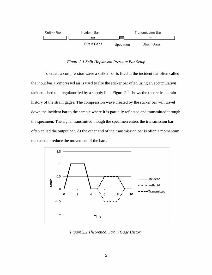
5
Figure 2.1 Split Hopkinson Pressure Bar Setup
To create a compression wave a striker bar is fired at the incident bar often called
the input bar. Compressed air is used to fire the striker bar often using an accumulation
tank attached to a regulator fed by a supply line. Figure 2.2 shows the theoretical strain
history of the strain gages. The compression wave created by the striker bar will travel
down the incident bar to the sample where it is partially reflected and transmitted through
the specimen. The signal transmitted though the specimen enters the transmission bar
often called the output bar. At the other end of the transmission bar is often a momentum
trap used to reduce the movement of the bars.
Figure 2.2 Theoretical Strain Gage History
-1
-0.5
0
0.5
1
1.5
0 2 4 6 8 10
Stra
in
Time
Incident
Reflectd
Transmitted

6
The compression wave in the SHPB can be adjusted with the length or velocity of
the striker bar (3). The increased length corresponds to an increased signal duration, and
an increased velocity corresponds to an increased strain rate. These two parameters can
be adjusted to attain the desired conditions.
The length of the striker bar is limited by the length of the incident and
transmission bars, also known as the pressure bars. The striker bar can be no greater than
half the length of the pressure bars. This is because for data reduction there can’t be
overlap between the incident wave and the reflected wave. The length of the incident bar
limits the length of the compression wave. The longest compression wave that can be
measured is half the length of the incident bar. To adjust for some of these limitations
some investigators have varied the lengths of the incident and transmission bars so that
the incident bar is longer than the transmission bar (3; 4).
2.2.2 Instrumentation
Since the SHPB was first investigated there have been many different ways of
measuring the stains in the pressure bars. Kolsky used a capacitance instrumentation to
measure the properties in his first pressure bar (5). The most common way of measuring
the strain in the pressure bars is with strain gages (3).
There have been other ways of obtaining the material properties other than strain
gages. Some investigators have used transducers to measure the force and acceleration at
the sample boundaries (6). This allowed the investigator to use pressure bars made of
non-linear elastic materials. In this setup the transducers are close to the specimen, and
the forces that the transducers read are the forces the specimen is subjected to. With a
traditional strain gage at the center of non-linear elastic bars non-linear wave propagation

7
would have to be applied. Another method is to use quartz crystals close to the sample to
measure the forces on either side of the sample (7). This has been done to check for a
uniform stress distribution within the specimen.
There are different setups of strain gages that investigators have used. Depending
on the setup and what the investigator is interested in, it is common to see a quarter
bridge as well as a half bridge setups. The quarter bridge setup uses one strain gage. The
half bridge setup uses two strain gages on opposite sides of the bar. The half bridge setup
can be used for subtracting off the effects of bending. If the bars are straight and aligned
properly there should not be any bending so the quarter bridge setup should be sufficient.
In order to read the strain gage signals the signal needs to be amplified. There are
many different amplifiers used by investigators. It is important to have an amplifier that
has a sufficient frequency response since the experiment happens over a very short period
of time. It was found that a frequency response of 160 kHz at -3db was sufficient. The
amplifiers are then attached to a device used to read or display the signal. Some common
devices for displaying the signals are oscilloscopes and computers (3).
2.2.3 Equations
Once the signals have been captured the data needs to be reduced. A typical strain
history of a split Hopkinson pressure bar is shown in figure 2.3. There are three waves
that are recorded, the incident, reflected, and transmitted waves. The first and second
waves recorded on the incident bar are the incident and reflected waves respectively. The
first wave recorded on the transmission bar is the transmitted wave.

8
Figure 2.3 SPHB Strain Gage Readings of Phenolic Sample
The incident wave is the pulse that is induced by the striker bar. This pulse then
travels down the bar and is partly reflected and transmitted into the specimen. As the
transmitted pulse travels through the specimen it deforms the specimen. The transmitted
pulse then progresses into the transmission bar (3).
From the incident, reflected and transmitted strain waves the specimen stress,
strain, and strain rate can be calculated. There are several ways to develop the equations
for the split Hopkinson pressure bar. One way is to look at the forces on an element in the
specimen (8). Another way is to start from the wave equation (3). In this development the
latter will be shown.
Figure 2.4 Wave Directions in a SHPB
The wave equation is
-1.5E+03
-1.0E+03
-5.0E+02
0.0E+00
5.0E+02
1.0E+03
1.5E+03
0.0E+00 5.0E-05 1.0E-04 1.5E-04 2.0E-04 2.5E-04 3.0E-04 3.5E-04 4.0E-04
Stra
in (
in/i
n)
Time (s)
Incident Bar Strain Gage
Transmission Bar Strain Gage

9
2
2
2
2 1
t
u
Cx
u
o ’ 2. 1
where Co is the wave speed and u is the displacement. The solution to the wave equation
can be written as the sum of two waves, as
RIoo uutCxgtCxfu )()(1 2. 2
for the incident bar and as
To utCxhu )(2 2. 3
for the transmission bar. The subscripts I, R and T refer to the incident, reflected, and
transmitted waves respectively.
One dimensional strain is given by
x
u
. 2. 4
Applying this relation to equation 2.2 strain in the incident bar can be expressed as
RIgf . 2. 5
It can be shown that the time derivative of equation 2.2 leads to
)()(1 RIoo CgfCu . 2. 6
Performing a similar step with equation 2.3 gives
ToCu2 . 2. 7
Since equations 2.6 and 2.7 are true for all location in the incident and
transmission bars respectively they are true for the surfaces contacting the specimen.
Combining these equations and calculating strain by dividing by L the un-deformed
specimen length gives the specimen strain rate as

10
L
uu )( 21
.
2. 8
Substituting equations 2.6 and 2.7 into equation 2.8 results in
)( TRIo
L
C
. 2. 9
Using Hook's Law and the definition of compressive stress
E
A
F
, 2. 10
the force at each end of the specimen can be written as
)(1 RIAEF 2. 11
and
TAEF2 2. 12
where A and E are the bar cross-sectional area and modulus of elasticity. Equations 2.11
and 2.12 assume the incident and transmission bars have the same cross-sectional area as
well as elastic modulus.
When the specimen is in equilibrium the forces on each side of the specimen are
the same. Assuming the specimen is in equilibrium equation 2.11 and 2.12 are equal and
it follows that the transmitted strain is equal to the sum of the incident and reflected strain
histories shown as
)( RIT . 2. 13
Using the relation for the strains shown in equation 2.13, the strain rate in
equation 2.9 becomes

11
)(2
)( tL
Ct R
o,
2. 14
which is the strain rate in the specimen. Integrating this equation will yield the strain in
the specimen as
dL
Ct
t
Ro
0
)(2
)(
. 2. 15
The stress in the specimen can be obtained by dividing the force in equation 2.12
by the specimen cross-sectional area expressed as
)()( tEA
At T
s . 2. 16
The term As is the specimen cross-sectional area and A and E are the bar cross-sectional
area and modulus respectively. For the strain and stain-rate the wave speed Co can be
calculated as
ECo
, 2. 17
where ρ and E are the pressure bar mass density and modulus respectively.
These equations are based on the assumption that the forces at both ends of the
specimen are the same. In the case of soft materials this is not always true. Softer
materials tend to have slower wave speeds requiring a longer period of time for both
sides to be in equilibrium. With longer soft materials the specimen can’t achieve
equilibrium within the short time the stress is applied. Investigators have tried different
methods for insuring that the specimen is in equilibrium (4; 7; 9; 10; 11). It has been

12
noted that with thicker samples it takes longer for the sample to obtain stress equilibrium,
so thinner samples are often used.
Many soft materials and foams do not have constant volume under deformation.
This makes it difficult to find the true stress and true strain. Because of this engineering
stress and strain are used in this thesis. The stress and strain obtained from equation 2.15
and 2.16 are engineering stress and strain respectively.
2.3 Split Hopkinson Pressure Bar History
The first person to do work with pressure waves in bars was Bertam Hopkinson in
1914 (12). Hopkinson used a single bar with a sample fixed to the end of the bar using
grease. This bar assembly was suspended on two strings allowing it to swing. A projectile
was fired at the end of the bar using explosives. This impact created a compressive wave
that traveled down the bar. At the opposite end of the bar was a sample attached to the
bar with grease. The compressive wave would reach the end of the sample and as the
wave was being reflected at the end, some of the momentum would be trapped in the
sample causing it to fly off.
By varying the size of the sample and length of the compressive wave Hopkinson
could tune the bar so that all of the energy was transferred into the sample. He was able
to measure the energy remaining in the bar by suspending it on two strings and measuring
the pendulum swing of the bar assembly. The sample's momentum was measured using
ballistics jelly. The momentum could be determined by the distance the specimen was
projected into the jelly.

13
Figure 2.5 Hopkinson's Bar Setup
In 1949 Henry Kolsky developed what is now called the Split-Hopkinson Pressure
Bar or some call it the Kolsky bar (5). Kolsky used two bars in series with a thin sample
sandwiched in between. A projectile was fired into the first bar using explosives. He used
capacitance instrumentation to measure the deflection of the bars. For the incident bar he
measured the transverse deflection with a rod perpendicular to the bar. The transmission
bar’s deflection was measured at the end of the bar with a rod. The rod was attached to
one end of a capacitance plate. The capacitance of the plate would change as the distance
between the plates changed. Kolsk related the change in capacitance to the displacement
on the bars.
Using this deflection he calculated the strain in each of the bars by using linear
wave propagation theory similar to that in equations 2.14-2.16. He was able to measure
the high strain rate properties of several materials including rubber, copper, lead and
others.
Since Kolsky developed the Split-Hopkinson Pressure bar there have been many
improvements. Lindholm and Yeakley made alterations to the split-Hopkinson pressure
bar in order to test materials in tension as well as compression (13). In 1988 Khan and
Hsiao measured plastic waves in solids using resistance foil stain gages (14). The use of
strain gages to measure the strains in SHPBs has become quite efficient.

14
Many different materials have been characterized at high strain rates. Chou, et al.
investigated the high strain rate properties of different plastics including Nylon 6/6 (15).
They were looking at the temperature increase during high strain rate testing using
imbedded sensors for the temperature. A SHPB was used to test the plastics at high strain
rates by Chou.
There has been some work done in testing of soft materials. Chen, et al. has done
a lot of work testing soft materials (7). Chen, et al. also tested polyurethane with a SHPB
(4). In that investigation they were interested in the effect that density had on the high
strain rate behavior of polyurethane.
There are a few challenges that are associated with testing soft materials. These
challenges are discussed in section 2.4. An overview of different techniques for testing
soft materials was written by Song, et al. (10).
More sophisticated computers for the numerical analysis are now available to
investigators as well as better strain gages and faster signal conditioners. The SHPB has
become the most popular form of testing the behavior of materials at high strain rates.
2.4 Soft Materials SHPB Testing
2.4.1 Introduction
There has been quite a bit of interest in testing soft materials at high strain rates.
A lot of the interest is based on the increased use of soft materials in modern applications.
Often these soft materials are used in applications where the strain rate is quite high or
could be high in the case of an impact, for instance automobile safety equipment,
aerospace, sporting good applications, and much more. A good understanding and
accurate models are needed when designing applications that use these materials.

15
2.4.2 Problems Associated with Soft Material SHPB Testing
There are several techniques for characterizing soft materials the most common
being a Split-Hopkinson pressure bar. The SHPB allows the investigator to attain the
desired high strain rates. But there are several problems that are associated with testing
soft materials using a traditional SHPB.
There are two main problems encountered with testing soft materials with a split
Hopkinson pressure bar. The first is that the magnitude of the transmitted wave is small
and often difficult to distinguish from the base line electrical noise. Second, the elastic
impedance of a soft material is very low, which means that the velocity of the elastic
wave generated from the pressure bar travels much more slowly in the sample than the
bar. Third, the sample must be in a state of uniform stress for the reduction equations to
apply. Because of the low impedance and the soft characteristics of the material a
uniform stress may be difficult to obtain (3).
These problems need to be addressed in order to obtain accurate data. There are
several ways to mitigate some of these problems. Many of the methods have advantages
and disadvantages.
2.4.3 Signal to Noise Ratio
Low magnitude transmitted waves are often seen in SHPB testing of soft
materials. The problem with low magnitude transmitted signals is that the signal to noise
ratio can be so low that the signal is indistinguishable from the base line noise. There are
several things that investigators have done to increase the signal to noise ratio. Besides
changing sample geometry most of the other techniques fall into two categories, changing
the pressure bar material and, changing the bar geometry.
16
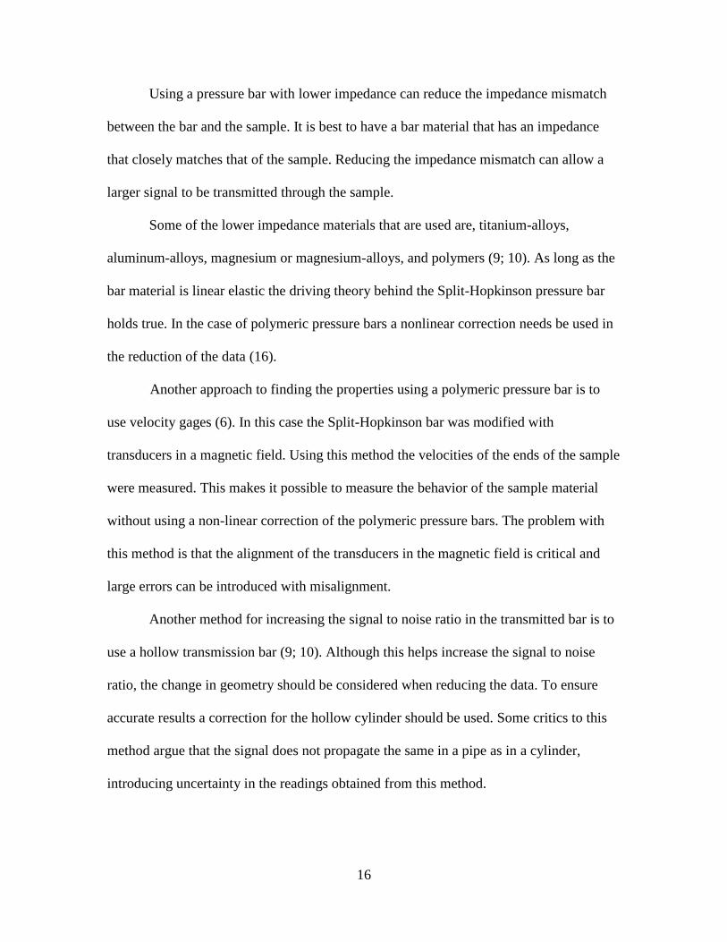
Using a pressure bar with lower impedance can reduce the impedance mismatch
between the bar and the sample. It is best to have a bar material that has an impedance
that closely matches that of the sample. Reducing the impedance mismatch can allow a
larger signal to be transmitted through the sample.
Some of the lower impedance materials that are used are, titanium-alloys,
aluminum-alloys, magnesium or magnesium-alloys, and polymers (9; 10). As long as the
bar material is linear elastic the driving theory behind the Split-Hopkinson pressure bar
holds true. In the case of polymeric pressure bars a nonlinear correction needs be used in
the reduction of the data (16).
Another approach to finding the properties using a polymeric pressure bar is to
use velocity gages (6). In this case the Split-Hopkinson bar was modified with
transducers in a magnetic field. Using this method the velocities of the ends of the sample
were measured. This makes it possible to measure the behavior of the sample material
without using a non-linear correction of the polymeric pressure bars. The problem with
this method is that the alignment of the transducers in the magnetic field is critical and
large errors can be introduced with misalignment.
Another method for increasing the signal to noise ratio in the transmitted bar is to
use a hollow transmission bar (9; 10). Although this helps increase the signal to noise
ratio, the change in geometry should be considered when reducing the data. To ensure
accurate results a correction for the hollow cylinder should be used. Some critics to this
method argue that the signal does not propagate the same in a pipe as in a cylinder,
introducing uncertainty in the readings obtained from this method.

17
2.4.4 Stress Distribution
Another problem with testing soft materials is the low inherent flow stress. The
low inherent flow stress can lead to a non-uniform stress distribution, which can cause
the characterization of the material to be inaccurate. The equations and theory behind the
SHPBs assumes that the sample has a uniform stress distribution (3).
To ensure that the soft sample is in uniform stress distribution the stress at both
sides of the sample can be measured. There are several methods that investigators have
used to do this. One method is the use of quartz crystal transducers on either side of the
sample (7). The quartz crystal has similar impedance to the aluminum bars that it is in
series with. Figure 2.5 shows the small disks on either side of the crystals installed to
protect the crystal. These transducers measure the force on either side of the sample. By
using pulse shaping techniques the two readings can be matched and a uniform stress
distribution obtained.
Figure 2.6 Quartz Crystal Transducer Setup
The disadvantage of using the quartz transducers to measure force is that the
transducers can disrupt the waves propagating through the bars. The increase in the
number of surfaces the wave is passing through can increase the amount of error
generated during a test.

18
There are other ways of determining if the specimen is in uniform stress
distribution. Song and Chen wrote an overview of different techniques for testing soft
materials (10). Besides the use of load cells to measure the stress at both end of the
specimen, the stress can be calculated using the force on the first face of the specimen.
This force is shown in equation 2.11. The incident and reflected waves can be added and
used to replace the transmitted wave in equation 2.16. The specimen’s uniform stress
distribution can be quantified using equation 2.16 and
))()(()(1 ttE
A
At RI
s . 2. 18
Dividing equation 2.16 by equation 2.18 gives the stress equilibrium factor as
RI
TEQ
.
2. 19
Figure 2.7 shows the numerator as 2 and the denominator as 1. The specimen is said to
be in perfect equilibrium when the stress equilibrium factor goes to unity (10).
Figure 2.7 Location of Stress for Stress Equilibrium Calculations
The advantage of using the incident and reflected waves to calculate the stress
equilibrium is that the SHPB does not have the added complexity of the load cells. The
downside is that when the transmitted wave is small the incident and reflected waves are
almost equal in magnitude and opposite in direction. Adding the incident and reflected
waves can introduce large amounts of error to the stress calculated.

19
Another way to reduce the time needed to attain uniform stress distribution is
changing sample size. Reducing sample length reduces the time needed to reach uniform
stress distribution. One of the effects of reducing sample length is that the strain and
strain rate also increase. Depending on what parameters the investigator is interested in
this could be beneficial.
2.5 Softball Background
Since softballs are a large focus of this thesis a discussion about the construction
of the softball is helpful. There are two factors that were compared in the studies done for
this thesis, the stiffness and the rebound properties of the softball.
2.5.1 Softball Properties
The stiffness of softballs can be measured by compressing the softball between
two flat plates a 0.25 inch and recording the load. This is referred to as the compression
of the softball. The softballs used in this thesis had nominal compression values of 300
lbs, 375 lbs, and 525 lbs. Balls are often sold with a maximum compression displayed on
the ball.
Another measure of softballs stiffness is called dynamic stiffness (DS). This is a
measure of balls stiffness during a collision with a cylinder. The cylinder has load cells
mounted opposite the collision site used for measuring the impact force. DS can be
calculated using the kinetic energy expressed as

20
22
2
1
2
1kxmv , 2. 20
where m is the mass of the ball, v is the velocity, and k is the dynamic stiffness. Force can
be expressed as
kxF . 2. 21
Using these equations the dynamic stiffness k can be expressed as
21
v
F
mk . 2. 22
The velocity is obtained by measuring the velocity before the collision and the force is
measured from the load cells.
The rebound properties of the softball are quantified using the coefficient of
restitution (COR). The COR is a measure of the energy retained after a collision with
possible values ranging from 0 to 1. The softballs used in this thesis had nominal COR
values of .40, .44, and .47. Balls are often sold with the nominal COR value displayed on
them. The decimal point is often left off.
2.5.2 Softball Construction
The softball is made from a rigid polyurethane foam center wrapped in a cover.
The covering is usually made from leather or synthetic and is often white or yellow.
Refer to figure 1.2 for a picture of the cross-section. One of the interests of this thesis is
to determine the impact properties of the foam center.
Rigid polyurethane foam is made by the reaction of polyisocyanates and polyols
in the presence of catalysts, surfactants, and blowing agents (17). The reaction is an
exothermic chemical reaction among liquid reactants. By varying the liquid reactants
different foam properties can be attained.

21
There are several different methods for preparing rigid polyurethane foam. The
methods are the block and sheet, poured in place, and sprayed. Softballs are made using a
poured in place method.
Softballs are constructed by mixing the polyisocyanates and polyols in a large
mixing tank. The batter, in the consistency of pancake mix, is poured into the molds and
then rotated while it cures. It takes about three minutes to cure. Since the reaction is an
exothermic reaction the temperature needs to be monitored while curing. There are
several variables that are adjusted to achieve different properties of the softball, cure
time, chemical makeup, and temperature (18).
2.5.3 Polyurethane Behavior
It is beneficial to know the expected behavior of polyurethane foam. Work was
done on the high strain rate properties of rigid polyurethane foam by Chen, et al. (4).
Chen found that polyurethane behaved similar to a structure rather than a solid. As the
foam is loaded the structure deforms slightly. Further loading causes the cell walls to
buckle and the behavior of the foam changes and becomes much softer until the cells
fully collapse, then the material becomes much stiffer again. Chen found that the
behavior of the foam and how it deforms through this general cycle is dependent on the
foam’s density. Chen’s graph for the foam that has a density similar to softball
polyurethane foam is shown in figure 2.8.

22
Figure 2.8 Dynamic Compressive Stress-Strain Curves for Polyurethane foam with a
density of 445 kg/m3 from Chen
2.6 Summary
Testing materials at high strain rates can be done quite effectively with a split-
Hopkinson pressure bar. The SHPB consists of two bars instrumented with strain gages.
A striker bar is fired at one end creating a compression wave that travels down the bar
and through the sample. These strain waves are read from the strain gages mounted on
the pressure bars. From these strain waves the specimen strain rate, strain, and stress can
be calculated.
The split-Hopkinson pressure bar was proposed by Kolsky and is an efficient way
of measuring the high strain rate properties of materials. There have been many
improvements to the split-Hopkinson pressure bar including resistance strain gages,
tension testing, and soft material testing.
There are several problems associated with testing soft materials with a split-
Hopkinson pressure bar. The most common problems are the signal to noise ratio and

23
attaining uniform stress distribution. A low signal to noise ratio can make it difficult to
obtain a large enough transmitted signal. Also reaching uniform stress distribution can
take longer with soft materials. Shortening the specimen length can help reduce the time
needed to reach a uniform stress distribution and it can help increase signal to noise ratio.
The coefficient of restitution and compression are common ways of quantifying
the behavior of softballs. The COR is a measure of the amount of energy retained after a
collision. The compression is a measure of the load needed to compress a softball 0.25
inches. The COR properties investigated for this thesis ranged from .40 to .47. The
compression properties ranged from 300 to 525.

24
3 Apparatus
3.1 Split Hopkinson Pressure Bar Setup
3.1.1 Introduction
The split Hopkinson pressure bar constructed for this project was designed to test
soft materials. The construction of the pressure bar is discussed in this section including
the structure and frame, instrumentation and electronics, and cannon setup.
3.1.2 Pressure Bar Structure and Frame
The split Hopkinson pressure bar was mounted on a framework constructed out of
Bosch tubing. The setup was mounted on a ten foot piece of Bosch 45X90 tubing. This
frame is shown in figure 3.1. There were three leg assemblies attached to the structure
using ninety degree gussets. Each of these leg assemblies had adjustable feet for leveling
the assembly. The cannon and pressure bars were mounted to the Bosch tubing using
custom made pillow blocks that have three setscrews for adjusting the alignment, figure
3.2. The cannon and the bars were each secured using two pillow blocks. The pillow
blocks used for the bars had polymer bearings to help reduce friction and reduce
conductivity to the frame. There was a momentum trap to constrain the motion of the
transmission bar consisting of a short two foot bar with a padded block shown in figure
3.3.

25
Figure 3.1 Split Hopkinson Pressure Bar Setup
Figure 3.2 Adjustable Pillow Blocks
Figure 3.3 Momentum Trap on Split Hopkinson Pressure Bar

26
3.1.3 Pressure Bar Electronics
The two bars of the SHPB were three feet long and 0.5 inches in diameter. The
bars were made of 6061 aluminum. At the center of each bar aligned with the length were
strain gages glued using Vishay Micro Measurements M-Bond 200 adhesive. A picture of
a mounted and wired strain gage is shown in figure 3.4. The strain gage was a Vishay
Micro Measurements EA-06-062AQ-350/W gage having a resistance of 350 Ohms. From
the strain gage there were small wires attached to soldering pads. These strain gages were
connected to a conditioner using shielded twisted pair strain gage wire number 326-BSV
from Micro Measurements.
Figure 3.4 Mounted and Wired Strain Gage
The conditioners used were 2310B signal conditioning amplifiers from Vishay
Micro-Measurements. These were picked because of the high frequency response of 160
kHz at -3db and 1000 gain. The excitation voltages of the conditioners were set to 10
volts. It was found that 15 volts tended to warm the strain gage causing the strain reading
to creep with time. The conditioners can be seen in figure 3.4. The conditioners were
connected to a PC using a connection block SCB-68 made by National Instruments. The
connection block was connected to a National Instruments analog-to-digital PCI-6111
board inside a Dell 4600 desk top computer. The NI PCI-6111 board could sample two
analog channels simultaneously at 5 mega-samples per second. The connection block
used for connecting the instrumentation to the A/D board can be seen in figure 3.5. The

27
A/D converter allowed the strain values from the conditioner to be read and recorded as
well as controlling the cannon pressure and valve firing.
Figure 3.5 Signal Conditioners
3.1.4 Cannon Setup
Figure 3.6 is a picture showing the control box setup, and figure 3.7 is a picture
showing the cannon setup with the different parts labeled. In order to fire the striker bar
the cannon was supplied with compressed air. There was a five gallon accumulation tank
that was used to supply the air for firing. The tank pressure was regulated using a
digitally controlled SMC regulator ITV3050-31N3CL4 which received input from the

28
PC. Connected to the tank was a MAC valve 57D-32-110AA used for firing the
compressed air.
The cannon barrel was attached to the valve using a 0.5 inch high pressure hose.
The steel cannon barrel was 24 inches long with a 0.5 inch bore. The MAC valve was
fired using a 24 volt signal supplied through a solid state relay. The control box is shown
in figure 3.6. In this figure the solid state relay can be seen as well as two power supplies
and the connection block.
Figure 3.6 Control Box

29
Figure 3.7 Cannon Assembly
3.2 Pressure Bar Operation
The operation of the split Hopkinson pressure bar is fairly simple. A detailed step
by step operating procedure can be found in appendix A. The pressure bar is controlled
using a LabVIEW vi named “Pressure Bar.vi”. There are several aspects about the
pressure bar that can be controlled using this front panel setup. The program is used to
save and crop the strain gage data as well as control the cannon pressure and firing.
Figure 3.8 shows a screen shot of the front panel setup.
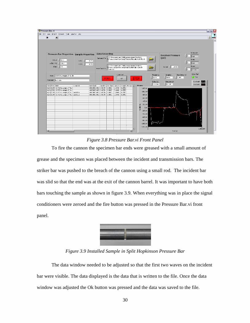
30
Figure 3.8 Pressure Bar.vi Front Panel
To fire the cannon the specimen bar ends were greased with a small amount of
grease and the specimen was placed between the incident and transmission bars. The
striker bar was pushed to the breach of the cannon using a small rod. The incident bar
was slid so that the end was at the exit of the cannon barrel. It was important to have both
bars touching the sample as shown in figure 3.9. When everything was in place the signal
conditioners were zeroed and the fire button was pressed in the Pressure Bar.vi front
panel.
Figure 3.9 Installed Sample in Split Hopkinson Pressure Bar
The data window needed to be adjusted so that the first two waves on the incident
bar were visible. The data displayed is the data that is written to the file. Once the data
window was adjusted the Ok button was pressed and the data was saved to the file.

31
3.3 Problems and Solutions
During construction of the SHPB there were several problems that were
encountered. This section discusses those problems and some of the steps taken to fix the
problems. The two main problems were signal noise and cannon alignment.
3.3.1 Noise Problems
As the SHPB was being debugged there was a fair amount of noise that was
observed. Several changes were investigated to reduce the noise, many of which had little
effect. The noise problems observed as well as the attempted solutions are discussed
below.
One of the first solutions investigated dealt with a grounding issue. There was a
poor ground between the electronics and the earth ground. After some investigation it
was determined that the supplied power was not connected to an earth ground. This was
solved by connecting to an electrical outlet located closer to the source that had a good
earth ground. This electrical outlet had been installed recently and complied with current
electric standards.
Another noise problem that was observed dealt with a signal spike that was
observed when the cannon valve opened and closed. There were several failed attempts to
solve this problem. It was determined that the signal spikes did not interfere with the data
that was being investigated. Some of the steps to eliminate or reduce this spike were, the
installation of a line snubber, and separating the power supplies to the valve and
regulator. The valve was on a switching power supply and the regulator and everything
else that needed power was connected to a linear power supply. This is why there are two
power supplies shown in figure 3.5.

32
When the split Hopkinson pressure bar was first built and tested, it was found that
the expected trapezoidal waves were disrupted by other large amplitude noise waves
within the time scale of the strain readings. At that time in the testing only one bar was
installed in the fixture. An example of the noise can be seen in figure 3.10. For the case
shown the excitation voltage was set at 2.5 volts. The incident and reflected strain
histories can be seen. By aligning the bars more precisely, using lubrication at the impact
location and specimen location, and using conditioners with larger excitation voltage of
10 volts and faster frequency response of 160 kHz at -3db, the noise was able to be
reduced.
Figure 3.10 Noise Problem with Incident Bar Impacted
This noise did not seem to be related to the output signal generated by the
amplifier. If the excitation voltage of the amplifier was turned off, this large amplitude
noise was still observed during an impact. A graph of this noise can be seen in figure
3.11. In this case the incident bar was the only bar impacted. The transmission bar is
plotted to see what the base line noise was like. The steps that were taken to solve this
problem were increasing the amplifier excitation voltage to 10 volts, remounting the
-1
-0.5
0
0.5
1
1.5
0E+0 1E-4 2E-4 3E-4
Stra
in G
age
Vo
ltag
e (
V)
Time (s)
Transmission BarIncident Bar

33
strain gages on the pressure bars, and installing new shielded strain gage wires. These
steps reduced the impact of the noise on the strain readings.
Figure 3.11 Zero Excitation Voltage Noise in Incident Bar
At one time during the investigation into this problem the voltage readings
obtained from the zero excitation voltage impact could be subtracted from the 2.5 volt
excitation voltage impact and a more defined curve could be observed. This was found to
be impractical since the noise generated from the zero excitation impact and the noise
within the 2.5 volt excitation impact was not always the same shape and amplitude. An
example of the result of the subtraction is shown in figure 3.12.
-1
-0.5
0
0.5
1
0.0E+00 1.0E-04 2.0E-04 3.0E-04
Stra
in G
age
Vo
ltag
e (
V)
Time (s)
Transmission Bar
Incident Bar

34
Figure 3.12 Subtraction of Excitation off and on
With further investigation to this noise problem it was determined that several
things did not seem to affect this impact noise. Rotating the bar so that the strain gage
was at different angles did not make a difference in the noise generated. The rotation or
axial alignment was to determine if the noise generated was caused by the strain gage
traveling through a magnetic field. Other areas that seemed to have little impact on the
noise problem were friction of the bearings, pressure bar material, and machining the
pressure bar ends square. These things did not have an observed impact although some
investigators have found a lack of friction and square bar ends to be important (3).
What has seemed to work the best to reduce this noise problem was to align the
bars and use only straight bars, grease the ends of the bar’s at the impact location and the
specimen location. To align the bars new pillow blocks were made that had adjustment
screws. This reduced the noise some but not as much as was hoped. It is believed that
these solutions reduce the noise problem because they help ensure linear wave
-1
-0.5
0
0.5
1
1.5
0.0E+00 1.0E-04 2.0E-04 3.0E-04
Stra
in G
age
Vo
ltag
e (
V)
Time (s)
2.5V Excitation
0 Excitation
Difference

35
propagation in the bars. The increased excitation voltage made a large improvement on
the noise reduction by increasing the amplitude of the desired strain readings.
3.3.2 Cannon Alignment
When the pressure bar was first designed, pillow blocks were machined to fit
rigidly in the grooves of the Bosch tubing. This was done to ensure proper alignment
since alignment is important to ensure linear wave propagation (3). Unfortunately the
original bars installed were not straight and variation in machining of the pillow blocks
caused a noticeable misalignment of the bars. The bore of the cannon and the bars also
did not align. A majority of the original testing was done with these misaligned bars.
Later the bars were replaced with straight steel bars and later with straight aluminum
bars. The straightness of the bars helped some, but there was still misalignment between
the bars and the cannon barrel. To fix these problem new pillow blocks were made with
three setscrews spaced at 60° around the pillow block enabling the bars to be aligned with
the cannon barrel.
Figure 3.13 Adjustable and Rigid Pillow Blocks
Another problem that had been noticed with the cannon barrel was that the bore
was machined too small. This caused the 0.5 inch striker bar to become stuck inside the
cannon when it was fired. To correct this problem the cannon barrel and the striker bars

36
were sanded to allow smooth travel while firing. As the cannon was used there had been
buildup of dirt or other debris. To fix this problem the barrel can be cleaned periodically
with a rod, sandpaper and a drill. Figure 3.14 shows the setup that was used to clean the
barrel.
Figure 3.14 Sanding the Barrel
3.4 Summary
The design and setup of the split Hopkinson pressure bar was presented along
with the operating procedure and some of the problems encountered during construction.
The split Hopkinson pressure bar was designed to test soft materials. This was
done by using shorter incident and transmission bar made from aluminum. The pressure
bars were instrumented with strain gages that were connected to a computer through
conditioners.
To operate the pressure bar a program was written in LabVIEW. This program
was used to control the firing speed by regulating the air pressure in a supply tank. Also
the LabVIEW program recorded the strain gage readings and saved those to a file for data
reduction.
Some of the problems encountered while constructing and debugging the SHPB
were electrical noise and cannon alignment. The electrical noise was reduced by fixing

37
grounding issues and increasing the excitation voltage. The cannon alignment was
improved by installing adjustable brackets for holding the pressure bars.

38
4 Experiments
4.1 Introduction
The impact properties of various softballs were tested. Softballs with different
stiffness and rebound properties were compared to determine what effect stiffness and
rebound properties had on their behavior. The procedures used for testing these the
materials is discussed in this chapter.
4.2 Verification
To verify that the split Hopkinson pressure bar was working data obtained from
the SHPB needed to be compared with data obtained from a working pressure bar. In
1973 Chou, Robertson and Rainey published an article where they tested Nylon 6/6 and
other polymers using a split Hopkinson pressure bar (15). They were looking at
temperature rise during testing. The sample they used was 3/8 inches in diameter and 1/2
inches in length. Using a specimen of the same size the stress strain obtained by Chou, et
al. was matched quite well. The data tested in the laboratory with the SHPB was
compared to that of data published by Chou in figure 4.1.

39
Figure 4.1 Engineering Stress and Strain of Nylon 6/6
The specimen measured in the lab was measured at an average strain rate of 644 s-
1. The data obtained by Chou was at a strain rate of 1250 s
-1. Although the strain rates are
different the data agree quite well. Chou had a total engineering strain of approximately
0.2, where the data measured was at a max strain of 0.054. The reason for the difference
in the strain rate and total strain was that Chou used a steel SHPB and an aluminum
SHPB was used for the measured curve. Using the same specimen dimensions as Chou it
was difficult to obtain the higher strain rate with aluminum bars. Because of the size of
the pressure bar the total strain of 0.2 could not be reached.
The curve given my Chou was displayed in true stress and strain but was
converted to engineering stress and strain. This was done so this thesis could be
consistent in displaying all the data in engineering stress and strain. The data displayed in
figure 4.1 is engineering stress and strain. Due to the strong correlation between the
measured values and those obtained by Chou the aluminum pressure bar data was
verified.
0
5000
10000
15000
20000
25000
0 0.05 0.1 0.15 0.2 0.25
Stre
ss (
psi
)
Strain (in/in)
Chou Curve
Measured Curve

40
4.3 Capabilities
4.3.1 Amplitude and Duration
There are several aspects about the split Hopkinson pressure bar that can be
varied in order to test different materials. There are two factors that have a significant
impact on the signal of the split Hopkinson pressure bar, the striker bar length and
velocity. As the striker bar length increases the signal duration increases. This is shown
below in figure 4.2. The trend of striker bar length to signal duration is linear and can be
seen in figure 4.3. This shows that the signal duration is proportional to striker bar length.
The striker bars used for this investigation are shown in figure 4.4.
Figure 4.2 Comparison of Striker Bar Length to Signal Duration
-1,500
-1,000
-500
0
500
1,000
1,500
-5E-18 1E-4 2E-4 3E-4 4E-4
Bar
Str
ain
(in
/in
)
Time (s)
9in Incident
9in Transmission
6in Incident
6 in Transmission
3in Incident
3in Transmission

41
Figure 4.3 Signal Duration Compared to Striker Bar Length
Figure 4.4 Aluminum Striker Bars
In order to attain similar amplitudes with different length striker bars the change
in striker bar mass needed to be considered. Since the velocity was regulated with cannon
pressure the pressure for a shorter striker bar needed to be decreased in order to match the
velocity of a longer striker bar. An equation was needed to relate the striker bar velocity
to the pressure.
0E+0
2E-5
4E-5
6E-5
8E-5
1E-4
1E-4
0 3 6 9 12
Sign
al d
ura
tio
n (
s)
Striker Bar Length

42
The velocity of the bar at the end of the cannon can be estimated using classical
kinematics. If pressure is constant the energy is expressed as
)(2
1 2
cLLPAmv , 4. 1
where m is the bar mass, v is the bar velocity, P is the pressure, A is the bar cross-
sectional area, L is the cannon length, and Lc is the length of the striker bar. It follows that
the calculated velocity at the end of the barrel can be expressed as
m
LLcPAv
)(2
. 4. 2
This equation is neglecting the frictional effects in the cannon.
Although this equation is an estimate and does not account for friction, it can be
used for comparisons between bar lengths to attain similar velocities. The pressure can be
taken as the measured tank pressure. The pressure in the cannon is unknown, but should
be less than the accumulator pressure and the cannon pressure should be constant.
Equation 4.2 was used to achieve similar amplitudes in figure 4.5.
The signal is also affected by the velocity of the striker bar. As the striker bar’s
velocity increases the signal amplitude increases. This can be seen in figure 4.5. To
increase the amplitude the cannon pressure was increased which increases the striker bar
velocity. The average bar strain is compared to the accumulator pressure in figure 4.6.
Although amplitude does not increase linearly with pressure there is a noticeable trend.

43
Figure 4.5 Comparison of Striker Bar Velocity Using a Striker Bar Length of 9 in
Figure 4.6 Strain Amplitude Compared to Accumulator Pressure
The general trends associated with the change in striker bar length and velocities
were as expected. The increased amplitude due to increased striker bar velocity and
increased duration due to increased striker bar length were discussed by Gray (3).
4.3.2 Shaping
Changing the shape of the incident wave changes the way the specimen is loaded
and can help in attaining uniform stress distribution. There are several techniques that can
-1,500
-1,000
-500
0
500
1,000
1,500
-5E-18 1E-4 2E-4 3E-4 4E-4
Bar
Str
ain
(in
/in
)
Time (s)
5psi Incident5psi Transmission10psi Incident10psi Transmission15psi Incident15psi Transmission
-1,400
-1,200
-1,000
-800
-600
-400
-200
0
0 5 10 15 20
Stra
in A
mp
litu
de
(in
/in
)
Pressure (psi)

44
be used to change the shape of the incident wave. One technique is to change the shape of
the striker bar. Another technique is to place something between the striker bar and
incident bar (10; 19). An example of a wave history where shaping has been used is
shown in figure 4.7.
Figure 4.7 Strain History in Pressure Bars with Shaping Used
To shape the waves tips were made for the striker bar. These tips were designed to
sit in front of the striker bar and change the shape of the loading side of the incident strain
wave. It was found that the gap between the striker bar and tip created excess noise and
made the data difficult to reduce. Figure 4.8 shows some of the different tips that were
used to shape the waves. Wave shaping using shaping tips was not used for the testing of
polyurethane due to the increased noise from shaping techniques caused by the alignment
as well as the joint between the shaping tip and striker bar.
-25
-20
-15
-10
-5
0
5
10
15
20
25
-300
-200
-100
0
100
200
300
0E+0 1E-4 2E-4 3E-4 4E-4 5E-4 6E-4
Tran
smis
sio
n B
ar S
trai
n (
in/i
n)
Inci
de
nt
Bar
Str
ain
(in
/in
)
Time (s)
Incident Bar
Transmission Bar

45
Figure 4.8 Incident Shaping Tips
The other technique for shaping the incident wave was the use of inserts between
the striker bar and incident bar. Copper was looked at for shaping. Different sizes of
inserts were applied for wave shaping. With copper it was found that the inserts also
created an increase in the signal noise.
It was determined that the signals that were being generated from the cylindrical
striker bar were sufficient for the characterization of polyurethane. Because of this,
further work in wave shaping was not conducted.
4.3.3 Polyurethane Specimen Size Effects
The specimen size was selected based on several factors. The signal transmission
and construction were the main factors. There were some investigative experiments
conducted to determine what length would enable signal transmission. The tools available
for specimen construction were also a factor.
At first a larger sample size was investigated. The size was 0.25 inches in
diameter and 0.25 inches in length. A picture of the sample is shown in figure 4.9. It was
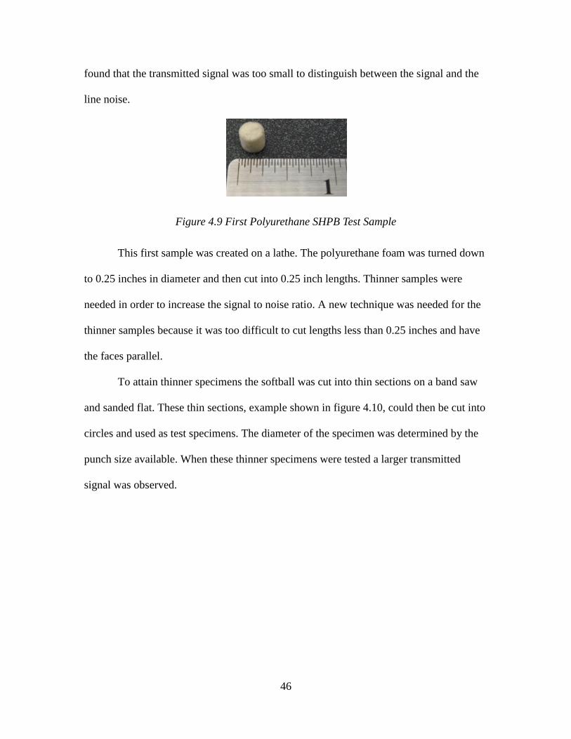
46
found that the transmitted signal was too small to distinguish between the signal and the
line noise.
Figure 4.9 First Polyurethane SHPB Test Sample
This first sample was created on a lathe. The polyurethane foam was turned down
to 0.25 inches in diameter and then cut into 0.25 inch lengths. Thinner samples were
needed in order to increase the signal to noise ratio. A new technique was needed for the
thinner samples because it was too difficult to cut lengths less than 0.25 inches and have
the faces parallel.
To attain thinner specimens the softball was cut into thin sections on a band saw
and sanded flat. These thin sections, example shown in figure 4.10, could then be cut into
circles and used as test specimens. The diameter of the specimen was determined by the
punch size available. When these thinner specimens were tested a larger transmitted
signal was observed.

47
Figure 4.10 Thin Specimen Construction
4.4 Polyurethane Introduction
4.4.1 Introduction
Softballs of different stiffness and rebound properties were compared in various
test throughout this thesis. There were five different models of softballs tested. Refer to
table 4.1 for a list of the models and advertized nominal properties COR and
compression.
Table 4.1 Ball COR and Compression
Manufacture Ball Code COR Comp.
Dudley WT11 ND Y-1 .44 525
Diamond 12RSC 44 .44 300
Worth SX44RLA3 .44 375
Diamond 12RFPSC 47 .47 375
Diamond 12RSC 40 .40 375
Softballs with different COR values were selected. To reduce the number of
variables balls with the same nominal compression were selected. This will help
determine how the COR effect different properties.

48
Another aspect about the softballs that was investigated was the stiffness.
Softballs with different stiffness properties having the same COR were selected. The
softballs were compared using dynamic stiffness (DS) but were selected based on their
compression values.
There is variation in the manufacturing process. A manufacture may advertise a
ball as .44 COR and 375 compression but the actual values of COR and compression are
usually different. Each ball that was tested was purchased in a lot of one dozen balls. Two
of each ball model were cut up for test specimens and six balls from each model were
tested to determine the lots average COR and compression. The average COR and
compression for each ball model are shown in table 4.2.
Table 4.2 Measured Average Ball Properties
Manufacturer Model Nominal COR/Comp
COR Average
Comp Average
DS Average
Dudley WT11 ND Y-1 .44/525 0.454 652 12259
Diamond 12RSC 44 .44/300 0.425 247 5424
Worth SX44RLA3 .44/375 0.442 360 6744
Diamond 12RFPSC 47 .47/375 0.462 338 5570
Diamond 12RSC 40 .40/375 0.426 440 7085
Upon examination of the average ball properties in table 4.2 it is evident that the
actual ball properties differ from the nominal values. Some ball models are closer to the
nominal values than others.
Other investigators have looked at testing polyurethane with a spit Hopkinson
pressure bar (4). They found that the properties of the polyurethane foam were dependent
on density. For a better comparison to this research the density has been calculated for
each ball by measuring the circumference and weight and calculating the density. These
results are shown in table 4.3.

49
Table 4.3 Ball Density
Manufacture Ball Code COR Comp Density oz/in3 (kg/m3)
Dudley WT11 ND Y-1 .44 525 .267 (462)
Diamond 12RSC 44 .44 300 .212 (367)
Worth SX44RLA3 .44 375 .211 (365)
Diamond 12RFPSC 47 .47 375 .208 (361)
Diamond 12RSC 40 .40 375 .204 (354)
4.4.2 Polyurethane Cell Comparison
Each ball has a slightly different density and different rebound and stiffness
properties. To understand how the cell structure affects these properties each ball was
looked at under a microscope. Pictures of each ball under M10 magnification are shown
below in figure 4.11. The view is about 1/32 by 1/32 inches.
The light circles in these pictures are foam cells that are open. It appears that the
cell size changes between ball models. Looking at specimens 12RSC 40 (40/375),
SX44RLA3 (44/375), and 12RFPSC 47 (47/375) it looks like the cell size increases as
COR increases. Comparing 12RSC44 (44/300), WT11NDY-1 (44/525), and SX44RLA3
(44/375) it looks like the compression also increase as cell size increases.

50
Figure 4.11 Magnified M10 Cross-Section of Ball Specimens
4.4.3 Finite Element Model
When the softball is impacted with the bat, the ball can experience strain at very
large strain rates. To model the bat-ball interaction, the properties of the softball at high
strain rates are needed. Using existing models the highest strain rate that is seen in the
ball is about 2500 s-1
. Figure 4.12 shows the strain rate as a function of time predicted by
a finite element model. The strain is 0.074 in/in at the peak strain rate.

51
Figure 4.12 Strain Rate in Ball Collision
Based on initial investigations the duration of the strain in the split Hopkinson
pressure bar test is 8.0E-5. This was based on tests using a nine inch striker bar. Figure
4.13 shows the same data as seen in figure 4.12 but with an adjusted time scale to match
what is seen in a SHPB test. Based on the data obtained from the initial finite elements
test the goal for the split Hopkinson pressure bar test was to obtain strain rates similar to
those seen in figure 4.13.
Figure 4.13 Strain Rate in Ball Collision Short Time Scale
The finite elements model used to calculate figure 4.12 and figure 4.13 was
created in LS-DYNA. These models are part of Warren Faber’s research (2). In figure
4.15 the mesh used to model the bat ball impact is shown. The lower mesh that is circled
0
500
1000
1500
2000
2500
3000
0 0.001 0.002St
rain
Rat
e (
1/s
)Time (s)
0
500
1000
1500
2000
2500
3000
0 0.00002 0.00004 0.00006 0.00008
Stra
in R
ate
(1
/s)
Time (s)

52
is the mesh that was used to display the strain rate in figure 4.13. On the left side is the
mesh before the impact and on the right the mesh is during the impact in the deformed
state.
Figure 4.14 Finite Element Ball and Bat Mesh, Before Impact (left), During Impact
(right)
4.4.4 Viscoelastic Response
Polyurethane is a viscoelastic material meaning the strain is time dependent and
stress dependent. Because the strain is dependent on time a viscoelastic model was used

53
to model the behavior of the polyurethane material. This viscoelastic model was also used
in the FEA model of the ball. Below is the development of the viscoelastic stress strain
equation.
The classical response of a linear viscoelastic material from a strain input is
described by
t
dtEt0
)()()(
,
4. 3
where E is the relaxation modulus (20). The relation between the elastic modulus and the
shear modulus is shown as
)1(2GE , 4. 4
where E is the elastic modulus, G is the shear modulus and ν is the poisons ratio.
The time dependent shear modulus using the numeric model is given by
t
o eGGGtG )()(.
4. 5
Combining equation 4.4 with equation 4.5 the elastic modulus can be expressed in terms
of the shear modulus as
))()(1(2)( 0
teGGGtE.
4. 6
The strain that is seen by the specimen is applied at a constant rate R and is zero
until time t

54
)()( tRtHt , 4. 7
where the step function H(t) is defined as 0 for t < 0 and 1 for t > 0. Taking the time
derivative of equation 4.7 gives
(t)Rt+RH(t)=(t) 4. 8
which is the strain rate. The function δ(t) is the derivative of the step function H(t) and is
zero everywhere except at t = 0 where it is 1.
Substituting equations 4.6 and 4.8 into equation 4.3 the stress can be expressed in
terms of the viscoelastic parameters G∞, Go, and β as
deGGGt
t
t
o (t))Rt+RH(t)())()(1(2)(0
)(
,
4. 9
where the terms ν and R are constants.
Since positive time is the only time of interest the step function H(t) is one for all
time being considered. Also the tδ(t) term is always zero since δ(t) is nonzero only when t
equals zero. Moving the constants out of the integral and applying the known values for
the delta function and the step function yields
deGGGRt
t
t
o
0
)( ))(()1(2)(
.
4. 10
Taking the integral then yields the stress in terms of known constants
)1()1(2)( to eGG
tGRt
.
4. 11
Equations 4.7 and 4.11 can be used to calculate the stress strain behavior of a
viscoelastic material. For polyurethane the parameters used to calculate the viscoelastic

55
stress strain response in the numeric model are shown in table 4.4. Using the parameters
in table 4.4 the stress strain curves were plotted in figure 4.15.
Table 4.4 Polyurethane Parameters for Viscoelastic Model
Properties Values
Dynamic Stiffness (lb/in) 4689 6227 9857 11339
Density (lb/in3) 3.975E-05 3.975E-05 3.975E-05 3.975E-05
Go (psi) 15000 20000 30000 35000
G∞ (psi) 680 1000 1800 2200
β (s-1) 68000 68000 68000 68000
R (s-1) 2500 2500 2500 2500
Figure 4.15 Predicted Viscoelastic behavior of Polyurethane
As the dynamic stiffness decreases the amplitude of the numeric stress strain
curve also decreases as seen in figure 4.15. This predicted curve will be compared to the
data collected in the discussion section of this chapter.
0
500
1000
1500
2000
2500
3000
3500
4000
0 0.1 0.2
Stre
ss (
psi
)
Strain (in/in)
DS 11339
DS 9857
DS 6227
DS 4689

56
4.5 Low strain Rate Testing
4.5.1 Low Strain Rate Test
For comparison with the high strain rate testing done with the SHPB, low strain
rate tests were conducted to compare the properties of the softballs. An MTS load frame
was used to measure the load and displacement of the samples. The setup used is shown
in figure 4.16. The sample was placed between two flat plates and compressed. Figure
4.17 shows the compressed state of the sample.
Figure 4.16 Low Strain Rate Compression Setup
Figure 4.17 Low Strain Rate Compressed Sample
The nominal dimensions of the sample cylinders that were compressed were 0.5
inches in diameter and 0.53 inches in length. The samples were made by cutting the

57
softball into long one inch square blocks using a band-saw. These long blocks were then
mounted into a lathe and turned down to 0.5 inches. The long cylinders were then cut to
length on a ban-saw. The ends were sanded flat to give a good surface to contact. The
ends of the sample were greased before placing them in the load frame. The samples were
compressed at a constant rate of 10 inches per second which gives a strain rate of 0.33 s-1
.
The displacement and load were read and recorded from the load frame using an attached
computer.
4.5.2 Stress Strain Results
From load-displacement data the engineering stress and strain were calculated and
plotted in figure 4.18 and figure 4.19. Figure 4.18 shows the stress strain curves for the
varied DS samples and figure 4.19 shows the stress strain curves for the varied COR
samples.
Figure 4.18 Varied DS at 0.33 s-1
Strain Rate
0
500
1000
1500
2000
2500
3000
3500
0 0.1 0.2 0.3 0.4 0.5 0.6 0.7 0.8
Stre
ss (
psi
)
Strain (in/in)
SX44RLA3
WT11 ND Y-1
12RSC 44

58
The general shape of the stress-strain curve is typical of rigid foams. This was
discussed in section 2.5.3. There is an initial section where the polyurethane foam
behaves rather linear, then after about 0.08 strain, the slope levels out. The last section
the slope increases again. In the first section the foam is withstanding the load placed on
it. After this point the cell walls began to buckle giving the flat region. The increased
amplitude at the end is because the cells have compressed and collapsed and the slope is
more a measure of the polyurethane material rather than the foam (4).
It is expected that the DS will have a noticeable impact on the stress-strain
behavior. The changes in behavior of different DS balls are expended to be proportional
to the measured DS.
Figure 4.19 Varied COR at 0.33 s-1
Strain Rate
In the varied COR graph it is expected that COR would not have a large effect on
the stress-strain behavior. This is because COR is a measure of the rebound properties not
of the materials stress-strain behavior. Upon examination of figure 4.19 it can be seen
that the curves are very similar. Refer to table 4.2 for the measured properties of these
0
200
400
600
800
1000
1200
1400
1600
1800
2000
0 0.1 0.2 0.3 0.4 0.5 0.6 0.7 0.8
Stre
ss (
psi
)
Strain (in/in)
SX44RLA3
12RSC 40
12RFPSC 47

59
balls. The difference between the curves in the varied COR graph can be attributed to the
variation in the DS not the variation in the COR. It is expected that for balls having the
same DS these curves would be the same.
4.5.3 Modulus
The modulus was found for the low strain rate stress-strain curves in figure 4.18
and figure 4.19. There are several sections in the stress-strain curve of the polyurethane
core. Each section has its own modulus. The modus that was calculated is for the initial
rise section that is linear. This linear section ends at a strain around 0.08. The modulus
values are shown in table 4.5. The measured COR and DS for each ball are also
displayed.
Table 4.5 Ball Modulus of Elasticity at 0.33s-1
Strain Rate
Manufacturer Model Nominal COR/Comp
COR Average
DS Average
Low Strain Rate Modulus
Dudley WT11 ND Y-1 .44/525 0.45 12259 7788
Diamond 12RSC 44 .44/300 0.42 5424 3041
Worth SX44RLA3 .44/375 0.44 6744 3637
Diamond 12RFPSC 47 .47/375 0.46 5570 2948
Diamond 12RSC 40 .40/375 0.43 7085 4101
There is a trend in the modulus associated with DS. This can be seen in figure
4.20. The modulus increased as the DS increased as expected.
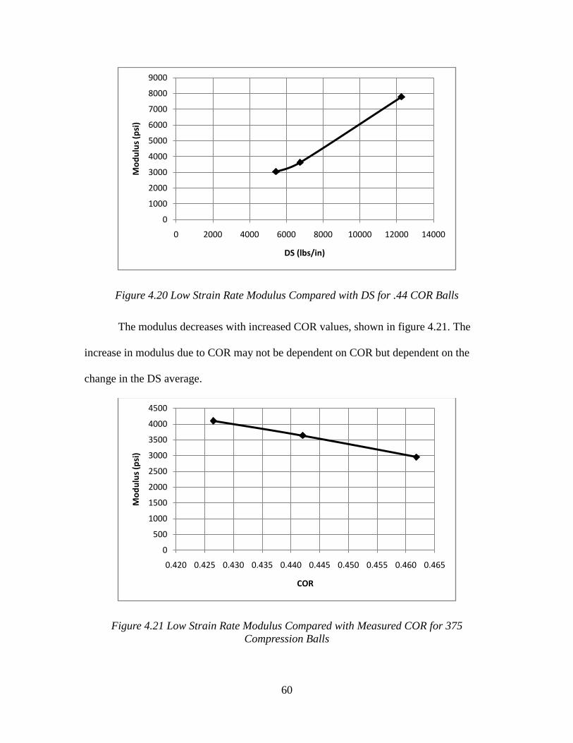
60
Figure 4.20 Low Strain Rate Modulus Compared with DS for .44 COR Balls
The modulus decreases with increased COR values, shown in figure 4.21. The
increase in modulus due to COR may not be dependent on COR but dependent on the
change in the DS average.
Figure 4.21 Low Strain Rate Modulus Compared with Measured COR for 375
Compression Balls
0
1000
2000
3000
4000
5000
6000
7000
8000
9000
0 2000 4000 6000 8000 10000 12000 14000
Mo
du
lus
(psi
)
DS (lbs/in)
0
500
1000
1500
2000
2500
3000
3500
4000
4500
0.420 0.425 0.430 0.435 0.440 0.445 0.450 0.455 0.460 0.465
Mo
du
lus
(psi
)
COR

61
4.5.4 Hysteresis
Another aspect of the softballs that was measured at low strain rates was the
hysteresis curve. This experiment was also done using the MTS universal testing
machine. The strain curves are shown in figure 4.22 and figure 4.23. The specimens were
loaded until they reached approximately 0.2 strain, then they were released at the same
rate they were loaded. The ramp rate for the testing machine was set at 1 in/min. The
nominal length of the specimens was 0.5 inches. The strain rate was 0.03 s-1
, this strain
rate was used so the compression could be stopped at desired deformations and to allow
recovery.
Figure 4.22 Hysteresis Comparison with Varied Stiffness
0
50
100
150
200
250
0 0.05 0.1 0.15 0.2 0.25
Stre
ss (
psi
)
Strain (in/in)
45 COR/12259 DS
44 COR/6744 DS
42 COR/5424 DS
0
50
100
150
0 0.05 0.1 0.15 0.2 0.25
Stre
ss (
psi
)
Strain (in/in)
42 COR/7085 DS
44 COR/6744 DS
46 COR/5570 DS

62
Figure 4.23 Hysteresis Comparison with Varied COR
The COR is a measure of the amount of energy retained in a system after a
collision. The hysteresis of softballs with the same COR should be the same. Softballs of
different stiffness traveling at the same velocity will have different displacements and
strains. The hysteresis displayed in figure 4.22 and figure 4.23 where loaded to the same
deformation. To compare balls with different stiffness the deformation should decrease
with increasing ball stiffness.
Using the energy of the ball
2
2
1kxE , 4. 12
where k is the DS and x is the deformation, the energy can be matched for each ball. DS
is the stiffness of the softball and this is different from the stiffness of the specimen
tested. Since the specimens tested are the same size the correlation between DS and the
stiffness is assumed to be the same for the softballs being compared. Once a desired
energy is selected the deformation can be calculated. This was done for the balls with
different DS and the result is shown in figure 4.24.
Figure 4.24 Constant Energy Hysteresis for Varied DS
-50
0
50
100
150
200
250
0 0.05 0.1 0.15 0.2 0.25
Stre
ss (
psi
)
Strain (in/in)
44 COR/6744 DS
45 COR/12259 DS
42 COR/ 5424 DS

63
Since there was some difference in the DS of the group of balls having different
COR, they were also loaded to displacements as a function of ball stiffness. These tests
were also measured using different deformations. The results for varied COR softballs
are shown in figure 4.25.
Figure 4.25 Constant Energy Hysteresis for Varied COR
The strain energy density of the curves shown in figure 4.24 and figure 4.25 was
calculated. The values are shown in table 4.6. The strain energy density for the varied
COR and stiffness are shown in figure 4.27 and figure 4.26.
Table 4.6 Strain Energy Density of Softballs at Constant Energy
Manufacture Ball Code COR DS (lbs/in)
Strain Energy Density (psi)
Dudley WT11 ND Y-1 0.45 12259 10.3
Diamond 12RSC 44 0.42 5424 7.7
Worth SX44RLA3 0.44 6744 7.8
Diamond 12RFPSC 47 0.46 5570 9.9
Diamond 12RSC 40 0.43 7085 9.6
0
50
100
150
0 0.05 0.1 0.15 0.2 0.25
Stre
ss (
psi
)
Strain (in/in)
44 COR/6744 DS
46 COR/7085 DS
42 COR/7085 DS

64
Figure 4.26 Strain Energy Density as a Function of DS for Varied DS Softballs
Figure 4.27 Strain Energy Density as a Function of COR for Varied COR Softballs
With the adjustment for constant energy the strain energy density is not constant
for different DS balls. With varied COR softballs it was expected that the strain energy
density would increase with increased COR. This was not observed in the results. There
could be several reasons for this. First the deformation that was predicted for constant
energy could be off due to the use of DS for the stiffness. The average DS may be
different from the DS of the particular ball tested. Another reason the results were not as
expected could be that the COR is tested at impact which takes place at high strain rates.
0
2
4
6
8
10
12
0 2000 4000 6000 8000 10000 12000 14000
Stra
in E
ne
rgy
De
nsi
ty (
psi
)
Dynamic Stiffness
0
2
4
6
8
10
12
0.42 0.43 0.44 0.45 0.46 0.47
Stra
in e
ne
rgy
de
nsi
ty (
psi
)
COR

65
The tests were conducted at low strain rates. The strain rate sensitivity of the balls is
probably the primary factor.
4.6 High strain Rate Testing
4.6.1 Specimen Construction
Because of the problems discussed in section 2.4.2 dealing with the testing of soft
materials, the test specimen needed to be thin. This was to ensure the specimen attained
uniform stress distribution more quickly. To make the specimens a thin slice of the
softball was cut using a band-saw. The tools used to construct the specimens are shown in
figure 4.28. A close up picture of the test specimen is shown in figure 4.29. The average
thickness of the test specimens was 0.08 inches. Once the section had been cut from the
softball the surface was cleaned with compressed air then sanded smooth. Using a hole
punch the specimens were stamped out of the softball section. The diameter of the
specimens was 0.44 inches.
Figure 4.28 Specimen Construction and Tools

66
Figure 4.29 High Strain Rate Test Specimen
4.6.2 Stress and Strain at High Strain Rates
Polyurethane is sensitive to temperature and humidity. Because of this the high
strain rate tests were done in an environment where the temperature and humidity were
constant and controlled. The temperature and humidity during the test were 72°F and
50% RH. There were many specimens made from each ball. Each specimen was only
tested once. The specimens were made from new balls so that the effects of wear from
impacts due to ball testing were not present.
The high strain rate tests were done using a SHPB with aluminum bars. The
pressure used for firing was 5 psi. The striker bar length was 9 inches. The excitation
voltage of the signal conditioners were 10 volts. An example strain reading from the
strain gages during a test is shown in figure 4.30. The incident and reflected curves are
quite large and the transmission curve is very small. Because the signal is so small there
is more variation due to signal noise.

67
Figure 4.30 Example Strain Gage Readings
The data was reduced using the equations in section 2.2.3, repeated here
R
o
L
C2
, 4. 13
dL
Ct
Ro
0
)(2
, 4. 14
t
s
EA
A
. 4. 15
The modulus used for the aluminum pressure bars was 10x106 psi, the density used was
2.53x10⁻⁴
(lb in/s)/in3. The calculated wave velocity (C0) was 1.99x10
5 in/s. The bar
diameter (A) was 0.5 inches. The properties of the specimen’s length (L) and area (As)
varied a little between each specimen but the average length was 0.08 inches and the
average area was 1.57 in2.
To check for uniform stress distribution the technique discussed in section 2.4.4
were employed. Equation 2.18 was used to calculate the stress at the incident side of the
-50
-40
-30
-20
-10
0
10
20
30
40
50
-8.E+2
-6.E+2
-4.E+2
-2.E+2
0.E+0
2.E+2
4.E+2
6.E+2
8.E+2
0.E+0 1.E-4 2.E-4 3.E-4 4.E-4
Tran
smis
sio
n B
ar S
trai
n (
in/i
n)
Inci
de
nt
Bar
Str
ain
(in
/in
)
Time (s)
Incident Bar Strain GageTransmission Bar Strain Gage

68
specimen. This stress was compared to the stress calculated from equation 4.16. An
example of this plot is shown in figure 4.31. In this graph “Stress T” is the stress obtained
from the transmission side of the specimen and “Stress I+R” is the stress obtained from
the incident side of the specimen. Because of the nature of polyurethane it was difficult to
obtain smooth curves for an accurate stress comparison. The oscillations seen in the
figure below are due to read error rather than actual oscillations seen by the specimen.
Figure 4.31 A Comparison of the Stress at Both Sides of the Specimen
In order to obtain an accurate stress strain curve the stress and strain needed to be
aligned properly. To do this the reflected and transmitted strain waves were plotted on the
same graph and aligned visually. The effect of misalignment is small. The alignment is
accurate to plus or minus 2x10⁻⁶
seconds. The effect of misalignment on the stress-strain
curve is shown in figure 4.32. For this figure an intentional misalignment was given to
demonstrate the effect of misalignment on the stress-strain curve. For polyurethane the
stress-strain curve is not sensitive to the alignment of the reflected and transmitted
curves.
-800
-600
-400
-200
0
200
400
600
800
1000
1200
1400
0.E+00 2.E-05 4.E-05 6.E-05 8.E-05 1.E-04
Stre
ss (
psi
)
Time (s)
Stress T
Stress I+R

69
Figure 4.32 Misalignment of Incident and Reflected Strain Signals
Based on the visual alignment of the curves the stress and strain were plotted
together to form a stress strain curve, an example curve is shown in figure 4.33. The
strain rate versus the strain was also plotted to show what the strain rate was for a given
stress and strain.
Figure 4.33 Stress and Strain Rate Compared to Strain for a Single Polyurethane Test
The stress strain curve is not smooth in figure 4.33. This is due primarily to the
low signal to noise ratio in the transmitted wave. The transmitted wave had very low
0
200
400
600
800
1,000
1,200
1,400
1,600
0.0E+00 5.0E-02 1.0E-01 1.5E-01 2.0E-01 2.5E-01
Stre
ss (
psi
)
Strain (in/in)
1.0E-5 sec.
0.5E-5 sec.
0
-0.5E-5 sec.
-1.0E-5 sec
-500
0
500
1,000
1,500
2,000
2,500
3,000
0.E+0
2.E+2
4.E+2
6.E+2
8.E+2
0.0E+00 5.0E-02 1.0E-01 1.5E-01 2.0E-01 2.5E-01
Stra
in R
ate
(1
/s)
Stre
ss (
psi
)
Strain (in/in)
Stress
Strain Rate

70
amplitude which meant the noise observed had a large impact on the stress. Because of
effect of noise on the signal six specimens were tested for each ball model.
The strain rate is controlled by two main factors, the speed of the striker bar and
the thickness of the specimen. The 9 inch striker bar was fired using a tank pressure of 5
psi. It was found that a tank pressure of 5 psi was needed to attain a sufficient velocity for
the striker bar to reach the end of the cannon barrel. To attain a lower strain rate a thicker
sample would be needed. Because of difficulty in obtaining transmitted signals with
thicker specimens a thin specimen was used. For these reasons it would be difficult to
obtain stress strain curves with this SHPB at lower strain rates.
The high strain rate stress-strain behavior of softballs were obtained for softballs
with varied COR values. The stress-strain behavior of the balls is shown in figure 4.34. It
was expected that the COR would not have an effect on the loading of the stress-strain
curve because it is a measure of rebound. This lack of change in the behavior is
noticeable. As expected the behavior changed very little based on the change in COR
values. The 42/7085 ball has a larger stress for a given strain, this was probably because
of the higher DS of 7085 rather than the COR.

71
Figure 4.34 Stress-Strain Curve at Strain Rate of 2780 s-1
for Varied COR Softballs
The high strain rate behavior of varied DS balls was also measured. It was
expected that as DS increased the response of the softball would also increase. This can
be observed in figure 4.35. As the DS increased the response of the softball increased.
Figure 4.35 Stress-Strain Curve at Strain Rate of 2780 s-1
for Varied DS Softballs
In each of the high strain rate tests there is a fairly linear region between 0 and 0.1
strain. The slope of the linear section in each ball is the high strain rate modulus. The
high strain rate modulus for each ball is shown in table 4.7.
0
200
400
600
800
1,000
0.00 0.05 0.10 0.15 0.20 0.25
Stre
ss (
psi
) av
era
ge
Strain (in/in) average
46/5570
44/6744
42/7085
-200
0
200
400
600
800
1,000
1,200
1,400
1,600
0.00 0.05 0.10 0.15 0.20 0.25
Stre
ss (
psi
) av
era
ge
Strain (in/in) average
45/12259
44/6744
42/5424

72
Table 4.7 High Strain Rate Modulus
Manufacturer Model COR DS
(lbs/in) High Strain Rate
Modulus (psi) Dudley WT11 ND Y-1 0.45 12259 12158 Diamond 12RSC 44 0.42 5424 4191 Worth SX44RLA3 0.44 6744 5114 Diamond 12RFPSC 47 0.46 5570 4796 Diamond 12RSC 40 0.43 7085 6104
There was a trend noticed in the high strain rate modulus of the varied DS balls.
As the DS increased that high strain rate modulus increased, the increase was not linear.
This trend is shown in figure 4.36. This trend demonstrates the expected increased
response seen in figure 4.35.
Figure 4.36 High Strain Rate Modulus with Varied Stiffness
There is a slight downward trend associated with the high strain rate modulus of
varied COR softballs. The trend is probably a result of the variations in the DS of the
balls used since there was a demonstrated trend associated with DS and the DS of the
softballs points to the downward trend shown in figure 4.37.
0
2000
4000
6000
8000
10000
12000
14000
0 2000 4000 6000 8000 10000 12000 14000
Mo
du
lus
(psi
)
DS (psi)

73
Figure 4.37 High Strain Rate Modulus with Varied COR
4.7 Discussion
4.7.1 Stress Increase with Strain Rate
Polyurethane is a viscoelastic martial. Using a viscoelastic model it has been
shown in section 4.4.4 that the properties of viscoelastic materials are rate dependent.
Based on this rate dependence the data obtained during the low strain rate test should be
lower than the data obtained during the high strain rate test. Figure 4.38 compares the
stress strain behavior measured during the two tests.
0
1000
2000
3000
4000
5000
6000
7000
0.42 0.425 0.43 0.435 0.44 0.445 0.45 0.455 0.46 0.465
Mo
du
lus
(psi
)
COR

74
Figure 4.38 Stress Strain Curve Strain Rate Comparison for 44/375 Ball
It can be seen in figure 4.38 that there is an increase in the slope of the curve as
strain rate increases. This increase was seen on all five ball models. The graphs of the
other four balls are shown in Appendix B. The increase at 0.2 strain for each ball model
is shown in table 4.8. The average increase at 0.2 strain is 42%. For most of the balls the
strain at 0.2 is on the plateau of the stress strain curve. This gives a comparison of the
stress increased needed to reach the plateau due to increased strain rate.
Table 4.8 Stress Change at 0.2 Strain Between Strain Rates of 2780 s-1
and 0.33 s-1
Manufacture Model COR DS (lbs/in) % Change
Dudley WT11 ND Y-1 0.45 12259 48%
Diamond 12RSC 44 0.42 5424 41%
Worth SX44RLA3 0.44 6744 34%
Diamond 12RFPSC 47 0.46 5570 42%
Diamond 12RSC 40 0.43 7085 47%
4.7.2 Modulus Increase with Strain Rate
The modulus was calculated for the tests conducted at strain rates of 0.33 s-1
and
2780 s-1
. The modulus for the low strain rate tests are shown in table 4.5 and the modulus
0
200
400
600
800
0.00 0.05 0.10 0.15 0.20 0.25
Stre
ss (
psi
)
Strain
2780 s-1
0.33 s-1

75
for the high strain rate tests are shown in table 4.7. The percent change in modulus for
each ball is shown in table 4.9. The average increase in modulus is 33%. This can be seen
in figure 4.39 and figure 4.40 where the modulus with varied comp. and COR are
graphed for high strain rate and low strain rate. The downward trend associated with the
varied COR could be due to the variations in the DS of those softballs.
Figure 4.39 High and Low Strain Rate Comparison for Varied Stiffness
0
2000
4000
6000
8000
10000
12000
14000
0 2000 4000 6000 8000 10000 12000 14000
Mo
du
lus
(psi
)
DS (psi)
Low strain rate
High strain rate

76
Figure 4.40 High and Low Strain Rate Comparison for Varied COR
Table 4.9 Modulus Percent Increase Due to Increased Strain Rate
Manufacturer Model COR DS (lbs/in) %
Dudley WT11 ND Y-1 0.45 12259 36%
Diamond 12RSC 44 0.42 5424 27%
Worth SX44RLA3 0.44 6744 29%
Diamond 12RFPSC 47 0.46 5570 39%
Diamond 12RSC 40 0.43 7085 33%
4.7.3 Viscoelastic Comparison
The viscoelastic stress-strain response is dependent on the dynamic stiffness of
softballs. This is shown in figure 4.15. These viscoelastic models used in finite element
models have had problems matching the observed behavior of softballs when the velocity
of impact is changed. A comparison between the viscoelastic model and the high strain
rate data is desired.
The measured stress strain behavior can be compared to the behavior predicted by
the viscoelastic model. The curves for the viscoelastic model are calculated with a strain
0
1000
2000
3000
4000
5000
6000
7000
0.42 0.425 0.43 0.435 0.44 0.445 0.45 0.455 0.46 0.465
Mo
du
lus
(psi
)
COR
High strain rate
Low strain rate

77
rate of 2500 s-1
. The average strain rates for the curves tested with the SHPB are 2780 s-1
.
A comparison between SX44RLA3 and the viscoelastic models are shown in figure 4.41.
Figure 4.41 .44/375 Ball Compared to the Viscoelastic Model
Since the DS of the SX44RLA3 ball is 6744 it should be above the viscoelastic
curve for DS 6227 not below. The other softball models are also graphed with the closest
DS curve. These graphs are shown in Appendix C. The viscoelastic model is over
predicting the amplitude of the stress strain curve. This could be why the viscoelastic
model is not matching up with the data observed.
The strain rate is changing throughout the impact of the softball. The curve in
figure 4.12 peaks around 2500 s-1
, but this is only for a small amount of time. The
coefficients used in the ball model were obtained experimentally in laboratory test. The
viscoelastic model when used in an FEA model predicts the performance of the bat and
ball quite well at the speeds the coefficients were obtained at. Because of this there is
some confidence in the viscoelastic model. Also the high strain rate behavior the model is
compared to was measured with and is believed to be accurate.
0
500
1000
1500
2000
2500
0 0.1 0.2
Stre
ss (
psi
)
Strain (in/in)
SX44RLA3
DS 6227

78
Using a strain rate that varies with time could help in matching the behavior of
material obtained at high strain rates. This was done for SX44RLA3 shown in figure
4.42. The average strain rate measured from the test was used as the R term in the
viscoelastic model. This is shown in figure 4.42 as the dotted line. This prediction of the
viscoelastic model is still over predicting the measured behavior of the softball.
Figure 4.42 Viscoelastic Comparison Using Varied Strain Rate.
Since the ball impact is at the high strain rates for a short time the viscoelastic
model may predict the balls behavior at a much lower average strain rate. The average
strain rate based on the data shown in figure 4.13, the average strain rate the ball sees is
around 1000 s-1
. The high strain rate data is graphed with the viscoelastic model for
several different strain rates in figure 4.43. By adjusting the strain rate R term the
measured stress-strain curve cannot be matched, also the measured data has a strain rate
of 2780 s-1
. In order to match the curves measured the other parameters in the viscoelastic
model need to be adjusted.
0
500
1,000
1,500
2,000
2,500
3,000
3,500
0
500
1,000
1,500
2,000
2,500
0.00 0.05 0.10 0.15 0.20 0.25St
rain
Rat
e s
-1
Stre
ss (
psi
)
Strain (in/in)
viscoelastic Model
SX44RLA3
SX44RLA3 Strain Rate

79
Figure 4.43 Viscoelastic Strain Rate Variation Compared to High Strain Rate Data for
SX44RLA3
To consider how a viscoelastic model might describe the measured ball response,
the viscoelastic parameters were varied to fit the measured response as shown in figure
4.44 - figure 4.48, the parameters used are shown in table 4.10.
Table 4.10 Viscoelastic Model Adjusted Parameters
Model DS R G∞ Go
WT11NDY-1 12259 2780 400 10000 40000 0.1
12RSC44 5424 2780 400 3500 40000 0.1
SX44RLA3 6744 2780 400 4200 40000 0.1
12RFPSC47 5570 2780 400 4000 40000 0.1
12RSC40 7085 2780 400 5200 40000 0.1
0
500
1,000
1,500
2,000
2,500
0.00 0.05 0.10 0.15 0.20 0.25
Stre
ss (
psi
)
Strain (in/in)
SX44RLA3 44/6744R = 2500
R = 1500
R = 1000

80
Figure 4.44 Viscoelastic Model of WT11NDY-1 46/12259
Figure 4.45 Viscoelastic Model of 12RSC44 42/5424
-200
0
200
400
600
800
1,000
1,200
1,400
1,600
1,800
0.00 0.05 0.10 0.15 0.20 0.25
Stre
ss (
psi
)
Strain (in/in)
WT11NDY-1 46/12259Model
-100
0
100
200
300
400
500
600
700
0.00 0.05 0.10 0.15 0.20 0.25
Stre
ss (
psi
)
Strain (in/in)
12RSC44 42/5424Model

81
Figure 4.46 Viscoelastic Model of SX44RLA3 44/6744
Figure 4.47 Viscoelastic Model of 12RFPSC47 46/5570
0
100
200
300
400
500
600
700
800
0.00 0.05 0.10 0.15 0.20 0.25
Stre
ss (
psi
)
Strain (in/in)
SX44RLA3 44/6744Model
0
100
200
300
400
500
600
700
800
0.00 0.05 0.10 0.15 0.20 0.25
Stre
ss (
psi
)
Strain (in/in)
12RFPSC 47 46/5570Model

82
Figure 4.48 Viscoelastic Model of 12RSC40 42/7085
4.8 Summary
To compare effects of varied stiffness and rebound properties in softballs several
tests were done. Tests at high strain rates, as well as tests at low strain rates were
conducted.
The split Hopkinson pressure bar setup was verified with the testing of Nylon 6/6.
The data collected for Nylon 6/6 was compared to data published for Nylon 6/6. It was
found that the published data and the measured were quite close.
The capabilities of the split Hopkinson pressure bar were discussed. The pressure
supplied to the cannon controlled the velocity of the striker bar. It was found that with
increased velocity the amplitude of the incident stain increased.
The duration of the incident pulse was found to be related to the striker bar length.
With increased length of the striker bar the pulse duration increased. Because of the
increased mass in longer striker bars the pressure had to be adjusted to attain the same
-200
0
200
400
600
800
1,000
0.00 0.05 0.10 0.15 0.20 0.25
Stre
ss (
psi
)
Strain (in/in)
12RSC40 42/7085Model

83
velocity. An equation was developed to approximate the pressure needed for the different
striker bars to reach the same velocity.
Different shaping techniques were discussed. Tapered tips were used to try and
change the shape of the incident wave. It was found that these tips introduced more error
and variations in the readings. Another method investigated to shape the incident wave
was the use of shaping samples between the striker bar and the incident bar. In this case it
was also found that the wave shaping caused more error and variations.
In the testing of polyurethane samples it was found that the length had a
significant impact on the ability to record a transmission wave. With longer samples the
transmission wave could not be distinguished from the line noise. By reducing the sample
length a larger amplitude transmission wave was recorded.
Comparing the cell size under magnification it was determined that as
compression increases the cell size also increased. It was also noted that for increased
COR the cell size increases.
A finite elements model was constructed and run by a third party. It was found
that the predicted strain rate that the ball sees is around 2500 s-1
. The strain at this point is
about 0.2. These predictions from the finite elements model were the target for the high
strain rate tests.
The viscoelastic model used in the finite elements model was looked at. The stress
and strain were graphed for different dynamic stiffness balls. A strain rate of 2500 s-1
was
used to construct these graphs.
Low strain rate tests were conducted to determine the stress strain behavior of the
rigid polyurethane foam. It was found that the slope of the stress strain graph starts out

84
linear. After the linear section the slope reduces for the majority of the deformation. At
larger strain the slope increases again. The modulus of the first section of the stress strain
graph was compared for the different ball models. It was found that the modulus
decreases with increased COR, and increases with increased stiffness. The hysteresis of
the ball models were also looked at. It was found that there was no trend for the
hysteresis of the balls based on COR, but it was found that the hysteresis increased with
increased stiffness.
The different softball models were cut and thin specimens were constructed from
each ball. These specimens were tested in the split Hopkinson pressure bar. It was found
that even though thin specimens were used the signal to noise ratio still was a problem.
Because of noise interference six tests were averaged for each ball model. The averaging
cleaned up the signals resulting in good curves. It was found that the COR did not seem
to have much of an impact on the stress strain at high strain rates. The stress strain
behavior was dependant on the comp of the balls.
It was found that the stress increased with strain rate. This was seen in all the ball
models. The increase in stress was measured at 0.2 strain and the average was found to be
42%. The modulus also increased with increased strain rate. The modulus increased by an
average of 33% for all ball models.
Comparing the high strain rate stress and strain with the viscoelastic model it was
found that the viscoelastic model was greater than the measured stress and strain. The
viscoelastic model parameters were changed to fit viscoelastic stress-strain curve to the
measured high strain rate stress-strain curve.

85
5 Summary and Future Work
5.1 Summary
The impact properties of polyurethane are important because of their use in
softballs. Several different softball models with different stiffness’s and rebound
properties were tested. These samples were tested at high strain rates.
An effective way of testing materials at high strain rates is with a split Hopkinson
pressure bar. The setup consists of two pressure bars with strain gages mounted in the
centers of each bar. The specimen is sandwiched between the two pressure bars and a
striker bar is fired at one end. This causes a compression wave to travel down the
pressure bars. Part of this wave is reflected and transmitted at the specimen. The strain
gages record the waves. Data reduction techniques are used to calculate the stress, strain
and strain rate in the specimen.
In order to test the polyurethane at high stain rates a split Hopkinson pressure bar
was built. The pressure bars were made of aluminum allowing for better signal
transmission with soft materials. These aluminum bars were instrumented with strain
gages connected to conditioners. A computer was connected to the setup and a program
was used to control the setup and record the strain readings.
The velocity of the striker bar was controlled with the pressure in the supply tank.
It was found that with increased pressure the signal read by the incident strain gage
increased. The duration of the strain was found to be related to the striker bar length. An
increased length corresponded to and increased duration.
A finite element model was used to estimate what the strain rate and stain
amplitude were during a softball impact. These values were used as the target values for
86
the high strain rate tests. The viscoelastic model used for generating the data in the finite
elements model was graphed for different balls. This was later compared to the data
obtained from the highs strain rate tests.
Tests were conducted to determine the base low strain rate behavior. The stress
strain curve was plotted for all the ball models investigated. It was found that the
modulus decreased with increased COR and increased with increased stiffness. The
hysteresis effect of the ball was also tested at low strain rates. It was found that COR had
no impact on hysteresis and the stiffness caused an increase in stiffness..
For the high strain rate testing thins specimens were constructed and tested in the
split Hopkinson bar apparatus. Averaging six tests for each ball model good stress strain
curves were obtained. It was found that the stress strain behavior was affected by the
stiffness much more than the COR.
Comparing low strain rate curves with high strain rate curves it was found that an
increased strain rate corresponded to an increase in stress and modulus. It was also found
that the stress in the viscoelastic model was much higher than the measured stress. The
viscoelastic model parameters were changed to fit the measured data. Although the
model did not match the data measured it worked for modeling the ball properties seen in
laboratory tests. This could be because the ball only experiences high strain rates for a
short period of time and the model is used for high strain rates.
5.2 Future Work
Based on the disagreement between the viscoelastic models and the measured
impact properties of the softball future work is needed to accurately model the behavior
of the softball. It would be beneficial to have the measured properties of the softball at

87
the average strain rate obtained from the bat-ball impact. Testing at this strain rate with
the SHPB setup discussed in this thesis was not possible due to the constraints of the
sample length and striker bar minimum speed.
It may help to do some modifications to the SHPB cannon to enable slower striker
bar speeds. It could also be beneficial to install load cells on either side of the sample
similar to the ones Chen used (7). If these adjustments to the SHPB don’t allow for
testing at the average impact strain rate then a drop test might help. It may also be helpful
to make adjusts in the viscoelastic model that match the tested data and accurately model
the ball in the FEA model.

88
6 References
1. Duris, Joseph. Experimental and Numerical Characterization of Softballs.
Washington State University. 2004.
2. Faber, W. Finite Element Modeling of Softballs. 2009. Personal Communication.
3. Gray III, GT. Classic Split-Hopkinson Pressure Bar Testing. ASM Handbook.
Materials Park : ASM International, 2000, Vol. 8, pp. 462-476.
4. High-strain-rate compressive behavior of a rigid polyurethane foam with various
densities. Chen, W, Lu, F and Winfree, N. 2002, Exp Mech, Vol. 42, pp. 65-73.
5. An Investigation of the Mechanical Properties of Materials at very High Rates of
Loading. Kolsky, H. 1949, Proceedings of the Physical Society of London, Vol. 62, pp.
676-700.
6. A Polymeric Split Hopkinson Pressure Bar Instrumented with Velocity Gages. Casem,
DT, Fourney, WL and Chang, P. 2003, Soc for Exp Mech, Vol. 43, pp. 420-427.
7. Dynamic Compression Testing of Soft Materials. Chen, W, et al. 2002, J Appl Mech,
Vol. 69, pp. 214-223.
8. Kaiser, MA. Advancements in the Split Hopkinson Pressure Bar Test. Virginia
Polytechnic Institue and State University. [Online] 1998.
http://soar.wichita.edu:8080/dspace/bitstream/10057/775/1/t05035.pdf.
9. Gray III, GT and Blumenthal, WR. Split-Hopkinson Pressure Bar Testing of Soft
Materials. ASM Handbook. Materials Park : s.n., 2000, Vol. 8, pp. 488-496.
10. Split Hopkinson Pressure Bar Techniques for Characterizing Soft Materials. Song, B
and Chen, W. 2005, Latin American Journal of Solids and Structures, Vol. 2, pp. 113-
152.

89
11. On the use of the Compression Split Hopkinson Pressure Bar to High Strain Rate.
Couque, H and Walker, JD. 1994, Journal de Physique, Vol. 4, pp. 23-28.
12. A Method of Measuring the Pressure Produced in the Detonation of High Explosives
or by the Impact of Bullets. Hopkinson, B. 1914, Proceedings of the Royal Society of
London, Vol. 89, pp. 411-413.
13. High Strain-rate Testing: Tension and Compression. Lindholm, US and Yeakley,
LM. 1968, Experimental Mechanics, Vol. 8, pp. 1-9.
14. On the Use of Electrical-Resistance Foil Strain Gages for Plastic-Wave Studies in
Solids. Khan, AS and Hsiao, C. 1988, Experimetal Mechanics, Vol. 28, pp. 254-258.
15. The Effect of Strain Rate and Heat Developed During Deformation on the Stress-
Strain Curve of Plastics. Chou, SC, Robertson, KD and Rainey, JH. 1973, Exp Mech,
Vol. 13, pp. 422-432.
16. A Three Dimensional Analytical Solution of the Logitudinal Wave Propagation in an
Infinite Linear Viscoelastic Cylindrical Bar. Zhao, H and Gray, G. 1995, J. Mech. Phys.
Solids, Vol. 43, pp. 1335-1348.
17. Backus, JK. Rigid Polyurethane Foams. [ed.] D Klempner and KC Frisch. Polymeric
Foams. New York : Oxford Univeristy Press, 1991, 5, pp. 73-94.
18. Smith, Kathy. Softball Manufacturing Techniques. July 21, 2009. Personal
Communication.
19. Tasneem, N. Study of the Wave shaping techniques of the Split-Hopkinson Pressure
Bar Using Finite Element Analysis. Witchita State University. [Online] 2005.
http://soar.wichita.edu:8080/dspace/bitstream/10057/775/1/t05035.pdf.

90
20. Gibson, Ronald F. Analysis of Viscoelatic and Dynamic Behavior. Principles of
Composite Material Mechanics. Second Edition. Boca Raton : CRC Press, 2007, pp. 377-
464.
21. The Velocity of Longitudinal Waves in Cylindrical Bars. Bancroft, D. 1941, Physical
Review, Vol. 59.

91
Appendix A
How to operate the Sport Science Lab Split Hopkinson Pressure Bar
The following are instructions on how to operate the SHPB that was built for this
thesis. These are the procedures that were followed for obtaining the data used for this
thesis.
Boot up and turn on procedure
There are several power strips and switches that need to be turned on for the
proper operation of this pressure bar. The following are the order that things should be
turned on. Refer to Figure A.1 for the placement of switches.
1. Power strip located on the back of the frame should be turned to the ON position.
2. Turn the computer on and allow it to boot up.
3. Open LabView and select “Pressure Bar.vi” from the list of recently opened vi’s.
4. Make sure the black switch located on the right front leg is in the on position.
5. Twist the red safety switch on.
6. Make sure both conditioners are on and the voltage is zeroed for both strain
gages.

92
Figure A.1 SHPB Switches
Pressure bar front panel operation
Now that the power is on and the computer is running, the LabVIEW software
needs to be opened. To run the LabVIEW program follow the steps below. Fig is a screen
shot of the LabView front panel.
1. Go to start and click on LabVIEW. This should open the program.
2. Select “Pressure Bar.vi” from the list of vi’s. This should open the control panel
for the split Hopkinson pressure bar.
3. Create a new summery file and wave file for saving the data.
4. Click on the folder button next to the summery file or wave file.
5. Create a new text document for each.
6. Select the newly created text document for the summery file and wave file.
7. Input the bar properties under the bar properties section.
8. Under the sample properties section put in the length and diameter of the sample.

93
9. Next set the tank pressure. If the tank pressure is too high it could damage the
bars and if it is too low the bar won’t make it to the end of the cannon barrel. It is
suggested to use a pressure between 5 and 10 psi.
10. Select an appropriate frequency and number of samples. These fields are located
above the “Strains” graph to the right of the screen.
11. Click the run button in the top left corner. It is a white arrow.
12. Care should be taken not to fire the bar while it is being loaded.
Figure A. 2 Pressure Bar VI Front Panel
Pressure bar firing procedure
Once the above is completed the pressure bar should be ready to fire. The
following is the firing procedure for the SHPB.
1. Select the appropriate striker bar.

94
2. Load striker bar into barrel and use loading rod to push to the back of the barrel.
3. Apply a thin film of grease between the barrel and the incident bar.
4. Apply a thin film of grease between the specimen and both the incident and
transmission bar.
5. Place the specimen between the incident and transmission bars. It should stick to
either bar due to the grease on the bar ends.
6. Place container under specimen and cover the specimen to prevent the specimen
from flying around the room.
7. Make sure the incident bar is very close to the barrel opening and that both bars
are contacting the specimen.
8. Press FIRE in the LabView window.

95
Appendix B
Below are graphs comparing high strain rate stress strain curves with low stress
strain curves for the softballs that were tested. The graph of the other ball that was tested
is shown in figure 4.38.
Figure B.1 Stress Strain Curve Strain Rate Comparison for 47/375 Ball
Figure B.2 Stress Strain Curve Strain Rate Comparison for 40/375 Ball
0
200
400
600
800
0.00 0.05 0.10 0.15 0.20 0.25
Stre
ss (
psi
)
Strain
2780 s-1
0.33 s-1
0
200
400
600
800
1,000
0.00 0.05 0.10 0.15 0.20 0.25
Stre
ss (
psi
)
Strain
2780 s-1
0.33 s-1

96
Figure B.3 Stress Strain Curve Strain Rate Comparison for 44/525 Ball
Figure B.4 Stress Strain Curve Strain Rate Comparison for 44/300 Ball
0
200
400
600
800
1,000
1,200
1,400
1,600
0.00 0.05 0.10 0.15 0.20
Stre
ss (
psi
)
Strain
2780 s-1
0.33 s-1
0
200
400
600
800
0.00 0.05 0.10 0.15 0.20 0.25
Stre
ss (
psi
)
Strain
.44/300
12RSC 44

97
Appendix C
Graphs of the high strain rate SHPB tests are compared to the viscoelastic model.
The viscoelastic model has a strain rate of 2500 s-1
. The parameters used for modeling the
viscoelastic behavior can be found in table 4.4. The high strain rate SHPB test had an
average strain rate of 2780 s-1
. The other graph that goes with this section is figure 4.41.
Figure C.1 .47/375 Ball Compared to the Viscoelastic Model
0
250
500
750
1000
1250
1500
1750
0 0.1 0.2
Stre
ss (
psi
)
Strain (in/in)
DS 4689
12RFPSC 47

98
Figure C.2 .44/300 Ball Compared to the Viscoelastic Model
Figure C.3 .40/375 Ball Compared to the Viscoelastic Model
-250
0
250
500
750
1000
1250
1500
1750
0 0.1 0.2
Stre
ss (
psi
)
Strain (in/in)
DS 4689
12RSC44
-500
0
500
1000
1500
2000
2500
0 0.1 0.2
Stre
ss (
psi
)
Strain (in/in)
DS 6227
12RSC40
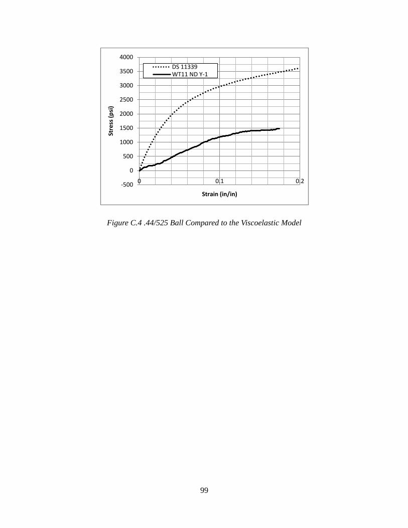
99
Figure C.4 .44/525 Ball Compared to the Viscoelastic Model
-500
0
500
1000
1500
2000
2500
3000
3500
4000
0 0.1 0.2
Stre
ss (
psi
)
Strain (in/in)
DS 11339WT11 ND Y-1