1

SAE 04ICES-239

Margin Determination in the Design and Development of a Thermal Control System

Daniel P. Thunnissen California Institute of Technology

Glenn T. Tsuyuki Jet Propulsion Laboratory, California Institute of Technology

Copyright © 2004 Society of Automotive Engineers, Inc.

ABSTRACT

A method for determining margins in conceptual-level design via probabilistic methods is described. The goal of this research is to develop a rigorous foundation for determining design margins in complex multidisciplinary systems. As an example application, the investigated method is applied to conceptual-level design of the Mars Exploration Rover (MER) cruise stage thermal control system. The method begins with identifying a set of tradable system-level parameters. Models that determine each of these tradable parameters are then created. The variables of the design are classified and assigned appropriate probability density functions. To characterize the resulting system, a Monte Carlo simulation is used. Probabilistic methods can then be used to represent uncertainties in the relevant models. Lastly, results of this simulation are combined with the risk tolerance of thermal engineers to guide in the determination of margin levels. The method is repeated until the thermal engineers are satisfied with the balance of system-level parameter values. For the thermal control example presented, margins for maximum component temperatures, dry mass, power required, schedule, and cost form the set of tradable system-level parameters. Use of this approach for the example presented yielded significant differences between the calculated design margins and the values assumed in the conceptual design of the MER cruise stage thermal control system.

INTRODUCTION

Spacecraft are complex multidisciplinary systems with a dozen or more subsystems. Thermal control is one example of such a spacecraft subsystem (discipline). This section begins with an overview of the preliminary design process for spacecraft thermal control. All complex multidisciplinary systems including spacecraft require engineers and designers to deal with uncertainty. A classification of uncertainty for complex multidisciplinary systems follows. This is the

classification that is applied to the thermal control system example in this paper.

PRELIMINARY DESIGN OF A SPACECRAFT THERMAL CONTROL SYSTEM

The purpose of a thermal control system is to maintain all of the components of a spacecraft within their allowable temperature limits for all operating modes of the vehicle and in all of the expected thermal environments. Since the environments experienced by spacecraft can largely vary, thermal designs have also varied significantly from spacecraft to spacecraft. The preliminary design of a spacecraft thermal control system can be viewed as consisting of five steps:1

1. Clearly understand the objective(s) and any key driving requirements of the mission

2. Develop a tractable design that meets those key requirements

3. Develop a preliminary schedule and cost estimate 4. Conduct and document the preliminary analysis 5. Identify possible development test to reduce

uncertainty In the first step, understanding the objective and its requirements may require meetings with program managers and other subsystem specialists. The second step may be an analysis, a set of tests, hand calculations, adapting a thermal design from a previous mission, or a combination of these activities. The third step typically entails the development of an outline of tasks required to support the job, criteria for determining if objectives are met, staffing levels, and a clear definition of what is expected from whom and when. The fourth step is the bulk of the thermal design effort. The thermal engineers must establish and maintain working relationships with the rest of the spacecraft design team; gather data and information about the system; decide on a thermal-design approach; develop, test, run, debug, and re-run thermal models; and periodically meet with management and their peers to evaluate the design progress. Documenting the design

2

and analysis includes a complete description of the final thermal design; a discussion of all the significant model inputs and assumptions; a summary of results; and a discussion of any significant concerns or recommendations. The fifth step addresses the primary limitation with analysis. There are uncertainties that may be quantified through test. The preliminary design of a spacecraft thermal control system is discussed in detail in Ref. 1.

UNCERTAINTY TYPES

Uncertainty in complex multidisciplinary systems can be classified into four types: ambiguity, epistemic, aleatory, and interaction.2 The following section provides a brief definition for each type of uncertainty.

Ambiguity

Because little precision is required for general communication, individuals often fall into the habit of using imprecise terms and expressions. When used with others who are not familiar with the intended meanings or in a setting where exactitude is important, this imprecision may result in ambiguity. Ambiguity can be reduced by linguistic conventions.

Epistemic

Epistemic uncertainty is any lack of knowledge or information in any phase or activity of the modeling process. The key feature that this definition stresses is that the fundamental cause is incomplete information or incomplete knowledge of some characteristic of the system or the environment. Epistemic uncertainty can be further classified into model, phenomenological, and behavioral uncertainty.

Model uncertainty is the accuracy of a mathematical model to describe an actual physical system of interest. Model uncertainty is associated with the use of one or more simplified relationships between the basic variables used in representing the ‘real’ relationship or phenomenon of interest. Phenomenological uncertainty arises whenever the design or development technique generates uncertainty about any aspect of the possible behavior of the system under development, operation, and extreme conditions. Phenomenological uncertainty is particularly important for novel projects or those which attempt to extend the ‘state of the art’. Behavioral uncertainty is uncertainty in how individuals or organizations act.

Behavioral uncertainty arises from four sources: design uncertainty, requirement uncertainty, volitional uncertainty, and human errors. Design uncertainty includes parameters over which the engineer or designer has control but has not yet decided upon. Design uncertainty is eliminated when a system is complete as all choices have been implemented. Requirement uncertainty includes variables that some organization or individual initially determines independently of the

engineer or designer. The question of whether an uncertain variable is a design or requirement depends on the context and intent of the model it is being used in and who the decision maker is. Volitional uncertainty is uncertainty about what the subject him/herself will decide. Other people’s future actions and conduct are not entirely predictable, particularly in dealing with other organizations. Finally, human errors occur during development of a system or project due to blunders or mistakes by an individual or individuals. Human errors are often difficult to estimate.

Aleatory

Aleatory uncertainty is inherent variation associated with a physical system or environment under consideration. Aleatory uncertainties can typically be singled out from other uncertainties by their representation as distributed quantities that can take on values in an established or known range, but for which the exact value will vary by chance from unit to unit or time to time.

Interaction

Interaction uncertainty arises from unanticipated interaction of many events and/or disciplines, each of which might, in principle, be or should have been foreseeable. Interaction uncertainty can also arise due to disagreement between informed experts about a given uncertainty (such as a design or requirement) when only subjective estimates are possible or when new data is discovered that can update previous estimates.

More detailed definitions and explanations of these uncertainties as well as an overview of uncertainty taxonomies in a variety of fields are provided in Ref. 2. Table 1 provides examples for each of these uncertainty types in the field of spacecraft thermal control. Since it is arguably more important to determine the significant sources of uncertainty in preliminary design than identifying and quantifying all uncertainty sources, Table 1 also indicates whether this form of uncertainty is viewed as significant and hence, included in the subsequent analysis.

3

Table 1: Examples of Different Uncertainty Types

Uncertainty Type Thermal Control Example Included in this Paper’s Analysis?

Ambiguity The maximum allowable temperature of the battery is 10 °C [anywhere? bulk average? etc.]

No

Epistemic Model The difference between the temperature predicted by an analytic

model and the actual flight measured temperature Yes

Phenomenological Thermal environment on a comet’s surface No Behavioral Design The choice between two different thermal paints for a

spacecraft’s exterior Yes

Requirement The spacecraft shall be able to reject up to 300 W of heat [and this requirement later changes to 350 W]

Yes

Volitional An analysis an engineer says he will perform but does not No Human errors A mistake in measuring the area of a thermal radiator No Aleatory Properties, such as emissivity or absorptivity, of a thermal paint Yes Interaction The combination of choice between two different thermal paints

and the fact that their properties are not certain Partly

MARGIN MANAGEMENT IN THERMAL DESIGN

Margin management in thermal subsystem design can be split into thermal margins and other margins. Thermal margins have been the topic of research and documented analysis for over three decades. Other margins are far less formal and developed. This section discusses both margin types.

THERMAL MARGINS

The current method for mitigating and propagating uncertainties in the temperatures a spacecraft will experience in its flight is through the use of thermal margins. Thermal margins are often further classified as a thermal uncertainty margin, a qualification thermal margin, or a protoqualification thermal margin.1

Thermal Uncertainty Margin

The thermal uncertainty margin is a margin of safey applied to worst-case analytic temperature predictions (from all mission phases) to account for uncertainties inherent in parameters such as complex view factors, surface properties, radiation environment, joint and interface conduction, and ground simulation.

A study of twenty Earth-orbiting satellite programs in the early 1970s concluded that an 11 °C margin was required to provide two standard deviations of confidence (95%) that on-orbit temperatures would be within predicted limits.3 This study is the basis of the MIL-STD-1540 analytical uncertainty margin of 11 °C.4 This margin is applied to predictions made by analytical models such as SINDA (System Improved Numerical Differencing Analyzer), the NASA-standard analyzer for thermal control systems, which have been correlated to thermal-balance test data. For an uncorrelated model, the margin increases to 17 °C. Very large discrepancies (40 to 50 °C) sometimes occur and one of the purposes of performing a system-level thermal-balance test is to

uncover these large, potentially catastrophic, errors before a spacecraft is launched. When the thermal uncertainty margin is added to worst-case temperature predictions, the thermal engineer has high confidence that design will be maintained within allowable temperature limits.

Qualification Thermal Margin

The classic qualification program entails the fabrication of an engineering and flight hardware. The reliability of the design is demonstrated by subjecting the engineering model to a qualification test. Typically, the qualification thermal test is conducted with margins ranging from 10 to 25 °C beyond the maximum and minimum allowable flight temperature limit. The flight model is then subjected to a flight acceptance test, which is typically performed with margins of 5 °C beyond the maximum and minimum allowable flight temperature limit. The qualification test demonstrates the relative reliability of the design while the flight acceptance test attempts to uncover any workmanship defects.

Protoqualification Thermal Margin

For cost and schedule reasons, hardware providers may chose to fabricate only flight units. These units are then qualified under a protoflight program. The temperature margin between protoflight testing and the maximum or minimum allowable flight temperature limit is usually less than the classic qualification test program. The intent of the protoflight test is to demonstrate the reliability of the hardware beyond expected flight temperatures without over-stressing the flight hardware.

It should be noted that if a component is heater controlled at the cold extreme, a 25% excess heater control authority is used in lieu of an 11 °C thermal margin. These three margins are described in more detail in Refs. 1 and 4.

4

OTHER MARGINS

Other uncertainties in thermal design such as the total mass and total power required are typically handled through managed system-level margins. Margins are also typically held for cost and schedule. These margins are variations in resources measured relative to worst-case expected values. Although the definition often differs from resource to resource, many margins are expressed as percentages:

100⋅−

=CBECBEWCEMargin%

current (1)

where WCE is the worst case estimate and CBE is the current best estimate.

Both thermal and other margins are implemented to allow the various elements of a design team to work in parallel as much as possible. By providing numbers with margin (“holding margin”), a team of a given subsystem or discipline is more insulated from changes occurring in other subsystems or disciplines and can proceed with their design and development. As the design progresses, CBEs of resources typically rise using up the margin that is being held. Significant design and management problems can occur when the rise in the CBEs is greater than the margin being held. On the other hand, holding too much margin early in project design causes the design to appear overdesigned, uncompetitive, or poorly managed. Determining the correct margin at various stages of the development is critical in determining the likelihood of success of the spacecraft design.

Both types of margins vary throughout the design and development and their allocation range from being capricious to “hope oriented” to overly conservative. For space systems in general, margins are allocated heuristically, based on historical data, or in a crudely quantitative manner, based on such concepts as design maturity and mission environment. Furthermore, margins maintained vary not only organization-to-organization, but from individual-to-individual (project manager-chief engineer, chief engineer-flight systems engineer, etc.) within an organization based on the risk tolerance of that organization or individual or both. Margins are supposed to account for all the uncertainties (aleatory, epistemic, behavioral, etc.) that were previously discussed. For example, the thermal uncertainty margin appears to primarily handle model (epistemic) uncertainty yet accounts for aleatory uncertainties as well. Qualification or protoqualification margin appears to primarily handle design and requirement uncertainty while qualification margin appears to tackle phenomenological and interaction uncertainties.

Although there was some statistical analysis into developing the thermal margins back in the early 1970s that was previously discussed, it is not clear that these

margins are still valid three decades later. Spacecraft structural and thermal analysis capabilities as well as understanding and knowledge of space have significantly increased. On the other hand, spacecraft power levels and complexity have also significantly increased during this same time. The current blanket method of applying 11 °C margins takes neither the positive nor the negative developments of the past three decades into account. Recent research has investigated whether 11 °C margins are appropriate, but only for two spacecraft.5 More troublesome are the other margins held during thermal design have little or no rigorous method behind their values. The unfortunate and often routine result is margins that are either blown in the design of spacecraft thermal control systems or overly conservative margins that penalize the entire spacecraft design and add little to advancing the fundamental understanding of these uncertainties.

SUMMARY OF METHOD

The following section describes a method for determining design margins in complex multidisciplinary systems. The method comprises six distinct steps: identification of tradable parameters, model formulation, classification of variables, probabilistic modeling of variables, Monte-Carlo simulation, and analysis. Each step is described in detail.

IDENTIFICATION OF TRADABLE PARAMETERS

The first step is the identification of tradable parameters. The design and development of a thermal control system is motivated by the overarching requirement of maintaining components within specified temperature ranges. The decision maker, who in this paper is assumed to be the thermal control project element manager, must understand the overall space system being analyzed to determine which parameters are truly important in satisfying the overarching requirement and associated subrequirements that will be placed on the thermal control subsystem. Engineering parameters will necessarily result from this analysis. Parameters such as schedule, cost, and risk, must usually be considered as well. The resulting list of tradable parameters helps guide the design and development of the complex multidisciplinary system.

MODEL FORMULATION

Once a list of tradable parameters has been identified, an analytic model must be generated to calculate each of these parameters. A model that determines engineering parameters often includes dozens or hundreds of equations and relations. A model that calculates the design and development schedule of an engineering system might subdivide the tasks required and estimate workforce requirements for each while a cost model might incorporate the schedule and include additional equations relating procurements, inflation, and burden factors. Determining how accurate models need to be to effectively determine the margin levels in

5

conceptual design is a critical issue and is partially addressed later in this paper for maximum temperatures of critical components.

CLASSIFICATION OF VARIABLES

Once models have been created for all desired tradable parameters, the variables used are classified. A thermal control system may have dozens, even hundreds, of these variables. Classifying the variables into their uncertainty types is useful in understanding their respective impact on the overall design. For this paper, aleatory and behavioral, specifically design and requirement, uncertainties were considered. Definitions and examples of each are provided in the Introduction.

PROBABILISTIC MODELING OF VARIABLES

The next step in the investigated method is probabilistic modeling of each variable previously described. Variables are characterized by a probability density function. Although normal (Gaussian) distributions are often the most common, other probability distributions are often used. For example, a uniform distribution may be used to model variables whose value is known to be within a range but not about any one particular value. An exponential distribution is often used in lifetime applications. A custom distribution might be used to represent design uncertainty. The probability density distribution applied to each variable may be determined from existing data, analogy, analysis, expert opinion, or a combination of these.

MONTE-CARLO SIMULATION

Once all the variables involved in the design have been given a probability density function, a Monte-Carlo simulation of the complex multidisciplinary system is performed. A Monte-Carlo simulation involves hundreds to thousands of simulations, each using different variables generated by their relevant probability distributions. For each simulation, the tradable parameters are recorded. Hence, the Monte-Carlo simulation generates probability density distributions of each tradable parameter. The more simulations performed, the smoother the resulting tradable parameter distributions. Statistical techniques can be used to estimate the required number of Monte Carlo samples.

ANALYSIS

With distributions of each tradable parameter provided by the Monte-Carlo simulation, an analysis of the complex multidisciplinary system is performed. Each tradable parameter distribution yields a mean and three percentiles. A percentile is defined as the value that is greater than a specified percent of all the values in a set. A percentile of 50 is simply the statistical median of a sample. Percentiles provide a confidence indication in the value of a tradable parameter. The 95, 99, and 99.9 percentiles of a tradable parameter provide a decision

maker with a low-, medium-, and high-confidence estimate in the probability that a tradable parameter will not be exceeded. The difference between these 95, 99, and 99.9 percentiles and the deterministic result provide the decision maker with a margin value to be maintained at the current stage of the design. The percent margin is this margin divided by the deterministic result (and multiplied by 100):

100⋅−

=det

detxproposed R

RPMargin% (2)

Once the distributions, means, and percentiles are analyzed, the decision maker may wish to investigate other uncertainties (such as model uncertainty) and combine these results with the Monte Carlo simulation. The decision maker may also wish to investigate which variables are driving one or more of the tradable parameters by performing a sensitivity analysis or investigate one or more different designs. As uncertainty in the values of variables decrease with time, the probability density distributions of each variable can be improved and updated. Repeating the process will yield updated margins as the design progresses. In summary, this method redefines the concept of design margin that was introduced earlier. Here, margins are a function of risk tolerance and are measured relative to mean expected system performance, not variations in design parameters measured relative to worst-case expected values.

APPLICATION OF METHOD

The investigated method is applied to a spacecraft thermal control system, specifically the thermal control system on the Jet Propulsion Laboratory (JPL)/NASA Mars Exploration Rover (MER) cruise stage. The primary objective of the Mars Exploration Rover (MER) project was the placing of two mobile science laboratories, MER-A (Spirit) and MER-B (Opportunity), on the surface of Mars in order to remotely conduct geologic investigations, including characterization of a diversity of rocks and soils that may hold clues to past water activity. The MER project used the 2003 launch opportunity to successfully deliver two identical rovers to different sites in the equatorial region of Mars in January 2004. The MER flight system consisted of four major components: an Earth-Mars cruise stage; an atmospheric entry, descent, and landing system or aeroshell (consisting of a heatshield and backshell); a lander; and a mobile science rover with an integrated instrument package as shown in Fig. 1.

6

Fig. 1: MER Flight System Configuration

During the interplanetary transfer to Mars, the cruise stage provided most of the traditional spacecraft subsystem functionality (such as propulsion, power, thermal, and attitude control).6 In particular, the thermal control system uses primarily passive techniques with thermostatic heaters to maintain allowable temperature limits during the cruise to Mars. A mechanically- pumped, single-phase fluid loop that is located throughout the entire flight system shuttles dissipated heat from the stowed rover. This waste heat is rejected from radiators on the cruise stage. Reference 6 discusses the MER mission in detail.

The analysis that follows was performed ex-post facto at an assumed period just before the preliminary design review (PDR). PDR is one of the most important periods for determining and updating margins in the development of a thermal control system. Although not performed in this paper, the method can be repeated at other times during design and development. It should also be stressed that the analysis in this paper is limited to the cruise stage, including the mechanically-pumped fluid loop. Although it is difficult to separate certain elements of the MER system as part of the cruise stage, the analysis described is limited to the cruise portion of the mission (from launch until arrival at the vicinity of Mars) insofar as possible. The results of the application of this method are compared to the actual MER thermal control system.

TRADABLE PARAMETERS

The tradable parameters identified for the MER thermal control system are component maximum temperatures, total system mass, total power required, schedule, and cost. Since the MER flight system comprised hundreds of distinct components, four “critical” components were explicitly tracked to minimize the analysis and documentary effort: the rover electronics module (REM), the rover battery, the small deep space transponder (SDST), and the solid-state power amplifier (SSPA). These four components are all located within the rover. A simple thermal analysis performed early in the design of MER concluded that the worst-case hot situation for these components would occur during cruise, soon after launch, when the spacecraft was in the vicinity of Earth.

The analysis performed in this paper corresponds to this worst-case hot situation. A similar simple analysis concluded the worst-case cold situation for these components would be on the surface of Mars, not during any of the cruise period. Hence, although the analysis could be completed for this separate situation on Mars, it was not done in this paper.

The total system mass is defined as the mass of all thermal control related equipment located on the cruise stage. Similarly, the total power required is the total power required by the thermal control system on the cruise stage. It should be noted that although not a significant portion of the total injected mass and total spacecraft power, the total mass of and power required by the thermal control system for MER were significant portions of the total cruise stage mass and power (30 kg out of a cruise stage total wet mass of ~240 kg, for example).

The schedule and cost are the total time and cost it takes to design, build, test, and deliver the thermal control system, respectively. At PDR, the MER project assumed “not to exceed” values for the four critical component maximum temperatures: 10 °C for the battery and 50 °C for the REM, SDST, and SSPA. Margins assumed on mass, power required, schedule, and cost during conceptual design were 5.5% (1.9 kg on 34.3 kg), 10% (6.0 W on 60.3 W), 4.3% (32 days on 738 days), and 26% (FY2003$2.6M on FY2003$9.9M), respectively. That is to say, the MER project did not anticipate the final cruise stage thermal control mass, power required, schedule, and cost to exceed 36.2 kg, 66.3 W, 770 days, and FY2003$12.5M, respectively.

The risk (the likelihood of catastrophic failure) of the thermal control system was not deemed important early in the design compared to the rest of the spacecraft. No major decisions concerning risk were made during design and development that significantly impacted the tradable parameters of component maximum temperature, system mass, power required, schedule, or cost. Hence, risk, a parameter that is often tradable in the design of other thermal control systems, is not tradable parameters for the MER thermal control system.

MODEL FORMULATION AND MAJOR ASSUMPTIONS

Physics-based models calculate the value of the five tradable parameters. Although these models are unique to the MER cruise stage design, they could be adapted for other spacecraft and applications although this was not investigated. This section begins with a description of the design and development of the MER thermal control system. A detailed description of the various models used follows.

MER Thermal Control System Design

The purpose of the MER cruise stage thermal control system was to maintain spacecraft component temperatures within their allowable range for the

7

duration of cruise. The original design philosophy for the MER spacecraft was a replica (“build-to-print”) of the similar 1996-1997 Mars Pathfinder design which performed successfully.7 Unfortunately, due to the fundamentally different configuration of the rover having all the “smarts”, as opposed to all the “smarts” on the lander electronics module for Pathfinder, the MER design had significant changes.

The thermal control system on the cruise stage of MER comprises the mechanically-pumped fluid loop known as heat rejection system (HRS), the shunt radiator, multilayer insulation (MLI), and miscellaneous components.

• The HRS in turn comprises radiators, tubing, a working fluid, an integrated pump assembly (IPA), associated support structure, and brackets and fittings.

o Radiators around the periphery of the cruise stage reject heat to deep space.

o Tubing routes the CCl3F working fluid (also known as chlorofluorocarbon 11, CFC-11, Refrigerant-11, and R-11) through the flight system. The tubing/working fluid transports much of the excess heat from the rover to the radiators via a combination of conduction and convection.

o The IPA consists of redundant pump motors, motor controllers, and thermal valves (that dictate amount of fluid flow to the radiators). Check valves are used to prevent back-flow from one pump side to the other.

o The associated support structure, in addition to housing the IPA, also contains two pyrotechnic valves, an HRS filter, and a pressure transducer and is hereafter referred to as the “IPA, vent, shunt limiter, and radiator” (IVSR).

• The shunt radiator rejects excess heat generated by the cruise stage solar arrays.

• MLI covers much of the cruise stage exterior and reduces the heat loss to deep space as well as reducing the absorbed heating rate of the spacecraft from solar insolation. Surface coatings and finishes provide means of achieving the desired heat rejection or retention. Platinum resistance thermometers are selected for Mars Pathfinder heritage.

• Miscellaneous components are located throughout the cruise stage and consist of temperature sensors, heaters, and thermostats. Kapton® film heaters provide a low mass implementation for maintaining hardware temperatures. In the case of the propellant lines, heater control is established by

flight software to retain in-flight adjustability. For other applications, high-reliability bimetallic thermostatics provide heater control.

The MER thermal control subsystem design and development is described in detail in other references.8,9

Engineering Model

The analytic engineering model determines the maximum component temperatures, total mass, and total power required by the thermal control system. The engineering model uses three distinct submodels to calculate each of these tradable parameters. A discussion of each model follows.

Component Maximum Temperatures

The temperatures of components throughout the spacecraft are determined using the network-style thermal simulator SINDA/FLUINT (version 4.6) via the graphical model development environment SinapsPlus®. Both software products are distributed by Cullimore and Ring Technologies, Inc., (Littleton, CO). Originally developed in the 1960s, SINDA (System Improved Numerical Differencing Analyzer) is now used by over 400 sites in the aerospace, energy, electronics, automotive, aircraft, and petrochemical industries for design, simulation, and optimization of systems involving heat transfer and fluid flow. It is the NASA-standard analyzer for thermal control systems.10 In particular, the reliability engineering module of SINDA/FLUINT was used. This reliability module wraps around existing SINDA code with only minor changes required as well as fitting within the framework of the method presented with limited post-processing additions.

As was previously mentioned, SINDA determines the temperature of all components on the spacecraft (via nodes) for the worst-case hot analysis being investigated. In the case of the MER SINDA model, approximately 900 nodes were used. This SINDA model was based on a previous Pathfinder model and was adapted to the MER mission. This worst-case hot analysis occurs at 1.01 astronomical units (AU) and a beta angle of 60°. The MER SINDA model includes a submodel for the HRS fluid loop. A detailed description of the MER SINDA model is beyond the scope of this paper.

Since tracking 900 temperatures and documenting the results within the framework presented is prohibitive, the temperatures of only four components were explicitly tracked in this analysis: the Rover Electronics Module (REM), the rover battery, the small deep space transponder (SDST), and the solid-state power amplifier (SSPA). These four components were critical components for the success of the MER mission. Specifically, the MER project wanted to be certain what the highest temperatures these components would attain and design the rest of the system accordingly. The MER project also wanted to know the coldest temperatures

8

these components would experience. However, as was previously discussed, this situation would not occur during cruise, but instead on the surface of Mars, and was not included in this analysis.

Total Mass

A separate model determines the total mass of the thermal control system (on the cruise stage). As was discussed earlier, the HRS consists of radiators, tubing, a working fluid, the IPA, the IVSR, and brackets and fittings. The total mass for q HRS radiators is:

radHRSradHRSradHRSradHRSradHRS tSqm _____ ρ⋅⋅⋅= (3)

The HRS tubing consists of several different lengths and/or diameters of tubing. The cross-sectional (material) area of tubing type j is:

( ) ( )[ ]22

4jin

jout

jtubingA φφπ

−⋅= (4)

The total material volume of the n different types of tubing is:

∑=

⋅=n

j

jtubing

jtubingtubing lAV

1 (5)

The total mass of the HRS tubing is therefore:

tubingtubingtubing Vm ρ⋅= (6)

The volume of the working fluid is:

( )∑=

⋅⋅=n

j

jtubing

jinfluid lV

1

2

4φπ

(7)

The density of the CCl3F working fluid is a strong function of both the temperature and pressure as shown in Fig. 2.11

105 106 107

240

260

280

300

320

340

360

380

400

420

440

Pressure (Pa)

Tem

pera

ture

(K)

200

200

400

400

600

600

800

800

1000

1000

1000

1200

1200

12001200

1400

1400 1400 1400

1600 1600 1600

Density (kg/m3)

200

400

600

800

1000

1200

1400

1600

Fig. 2: Density Contour Plot for CCl3F

With the density interpolated from the data of Fig. 2, the mass of working fluid can be found:

( )loadedloadedfluidfluidfluid pTVm ,ρ⋅= (8)

Although it is possible to develop expressions for the mass of the IPA, the IVSR, and brackets and fittings from their respective components, this was not done. Hence, the total mass of the HRS is:

fb

IVSRIPAfluidtubingradHRSHRS

m

mmmmmm

&

_

+

++++= (9)

Although it is possible to develop an expression for the mass of the shunt radiator this was not done. The total mass of the z different types of MLI is:

∑=

⋅=z

k

kMLI

kMLIMLI Sm

1ζ (10)

The mass of the miscellaneous components is:

thermostatthermostat

heaterheatersensorsensormisc

mqmqmqm

⋅+⋅+⋅=

(11)

Hence the total mass of the (cruise stage) thermal control system is:

miscMLIradshuntHRStotal mmmmm +++= _ (12)

MATLAB® was used for calculating the tradable parameter mass although virtually any mathematical modeling software could be used. MATLAB® was chosen since the overall structure of the analysis (several MATLAB® m-files) was created for a similar uncertainty analysis and modified for this analysis.12

Total Power Required

The tradable parameter total power required is the power required by the pump that moves the working fluid around the HRS in addition due to the miscellaneous components that draw power when operating. The power required to drive the pump in turn is a function of the pressure drop through the HRS tubing. The pressure drops through the HRS tubing from viscous friction and mixing losses. The flow rate of the working fluid in each tubing section is:

jtubing

fluidjfluid A

Gv = (13)

The viscosity of the working fluid is a function of temperature:

9

( ) cTbTafluid T

+⋅+⋅⋅=2

10001.0µ (14)

where a, b, and c for CCl3F are 3.183(10)-6 K-2, -0.006881 K-1, and 1.394, respectively.13 It should be noted that the viscosity calculated in Eq. (14) is metric unit specific (viscosity in kg/m-sec).

Assuming the temperature and pressure of working fluid does not vary significantly through the tubing, the Reynolds number through each tubing section is:

( )( )opfluid

jin

jfluidloadedopfluidj

TvpT

Reµ

φρφ

⋅⋅=

, (15)

The friction factor through each tubing section is a function of the Reynolds number. If the Reynolds number is below ~2000 in the tubing section the flow is laminar and the friction factor is:

200064<= j

jj ReRe

f φφ

(16)

If the Reynolds number is greater than ~2000 in the tubing section the flow is turbulent and the friction factor is:14

( ) 2000316.0 41>⋅=

− jjj ReRef φφ (17)

The pressure drop through each tubing section is:15

( ) ( ) jin

jtubingj

fluidloadedopfluidjj

tubing

lvpTfp

φρ ⋅⋅⋅⋅=∆

2,21

(18)

The pressure drop in the return bends is:15

( )

( ) ( ) bendsretfluid

loadedopfluidbendsretbendsret

lv

pTfqp

_

2

__ ,21

φ

ρ

⋅

⋅⋅⋅⋅=∆ (19)

where the barred quantities are the mean values over the entire length of tubing since bends are placed throughout the length of tubing. The expression for the pressure drop in the elbow bends is similar:

( )

( ) ( ) bendselbfluid

loadedopfluidbendselbbendselb

lv

pTfqp

_

2

__ ,21

φ

ρ

⋅

⋅⋅⋅⋅=∆ (20)

In this analysis, the equivalent length over diameter for the return bends and elbow bends were assumed to be 50 and 30, respectively.

Lastly, the pressure drop due to expansion or contractions between tubing sections are given by:1

( ) ( )

( )21

21

2,

21

,21

_

_

+⋅⋅⋅=∆

−⋅⋅⋅=∆

+

+

jfluid

jfluid

loadedopfluidconj

jfluid

jfluidloadedopfluidexp

j

vvpTkp

ncontractio

vvpTkp

expansion

change

change

ρ

ρ

φ

φ

(21)

The expansion and contraction conical loss coefficients were assumed to be 0.02 and 0.7, respectively.

Hence, the total pressure drop through the HRS tubing is the sum of these individual pressure drops:

∑

∑−

=

=

∆

+∆+∆+∆=∆

1

1_

__1

n

j

jchange

bendselbbendsret

n

j

jtubingtotal

p

pppp

φ

(22)

The mass flow rate through the HRS tubing is:

( ) fluidloadedopfluidfluid GpTB ⋅= ,ρ (23)

The hydraulic power and the total power of the pump are therefore:16

( )

overall

hydraulicpump

loadedopfluid

fluidtotalhydraulic

PP

pTBp

P

η

ρ

=

⋅∆=

, (24)

The total power required by other thermal control components is:

busthermostatonthermostat

heateronheatersensoronsensormisc E

Iq

IqIqP ⋅

⋅+

⋅+⋅=

_

__ (25)

Finally, the total power required by the thermal control system is the sum of the pump and miscellaneous component powers:

miscpumptotal PPP += (26)

MATLAB® was used for calculating the tradable parameter power required.

10

Fig. 3: Baseline Schedule (Abbreviated)

Schedule and Cost Models

A schedule model was developed to determine the time in workdays required to design, develop, integrate, test, and deliver two cruise stage thermal control systems (MER-A and MER-B). A nominal, deterministic schedule of 90 individual tasks was created. The nominal, deterministic schedule assumes no uncertainty in the task durations and all slack/margin in the schedule was removed. An abbreviated version of this schedule (~30 of 90 total tasks assumed) is shown in Fig. 3.

The duration and workforce required is then estimated for the tasks. Ideally this is done for each task listed but often, because of time and resource constraints, is done only for the rolled-up (summary) tasks. Table 2 lists this workforce allocation of individuals for the various tasks that comprise the MER thermal control system development.

A cost model was developed to determine the total inflated cost required to design, develop, integrate, test, and deliver two cruise stage thermal control systems

(MER-A and MER-B). The cost model uses the time and workforce estimates generated by the schedule model. The workforce is separated into two categories for cost estimation: staff and services. Staff is defined as employees of the organizational division tasked to design and build the propulsion system. Services is defined as either another division of the organization (or an entirely separate organization) tasked to assist in the design and development of the thermal control system. The inclusion of services in the cost model is representative of current industry practice where one organization often does not have the capability or workforce to complete the entire design and development themselves. The workforce types, their classification, and their assumed annual salary are provided in Table 3.

The total workforce time of each individual for each task is determined by the schedule model and the workdays per month is set to 20.5 in this analysis. The cost model also includes procurement and travel expenses which are summarized in Table 4.

Table 2: Workforce Estimate Workforce Member Task Names (% of Full-time Work Allocated) Blanketing ATLOa engineer Thermal Blankets (50) Blanketing technician Fabricate Cruise Stage Blankets (200) CADb Designer Perform HRS Design & Coordinate Implementation (50)

Formulate Hardware Fabrication & Assembly Approach (50) Cognizant engineer Spacecraft Hardware Lead (50)

Develop Test Plan/ Procedure – Flight 1 & Flight 2 (100) Prepare, Conduct, & Document Flight 1 & Flight 2 STT(100)

Cruise-stage HRS technician Fabricate Cruise Stage HRS Parts (75) Fabricate Rover HRS Parts (150)

11

Workforce Member Task Names (% of Full-time Work Allocated) Fabricate Lander HRS Parts (50) Assemble Cruise Stage HRS – Flight 1 & Flight 2 (800)

Contract Technical Monitor (CTM) - Heaters Flight Electrical Heaters (20) CTM - IPA IPA Contract (100) CTM - Temperature Sensors Flight Temperature Sensors (20) CTM - Thermostats Flight Thermostats (20) Design engineer CEDLc Design & Analysis (200)

Perform HRS Design & Coordinate Implementation (100) Formulate Hardware Fabrication & Assembly Approach (100) Fill & Charge HRS – Flight 1 & Flight 2 (100)

GSE engineer HRS GSE – Flight 1 & Flight 2 (50) GCU GSE – Flight 1 & Flight 2 (50)

GSE/ATLO technician Operate HRS GSE – Flight 1 & Flight 2 (100) Operate GCU GSE – Flight 1 & Flight 2 (100)

HRS ATLO engineer Install Lander HRS – Flight 1 & Flight 2 (100) Fill & Charge HRS – Flight 1 & Flight 2 (100)

Integration & Test (I&T) engineer IVSR#1 – Flight 1, IVSR#2 – Flight 2, IVSR#3 – Flight Spare (100) Perform HRS Design & Coordinate Implementation (100) Formulate Hardware Fabrication & Assembly Approach (100) Fabricate Cruise Stage & Rover HRS Parts (100) Assemble Cruise Stage HRS – Flight 1 & Flight 2 (100) Develop Test Plan/Procedure – Flight 1 & Flight 2 (100) Prepare, Conduct, & Document Flight 1 & Flight 2 STT (100)

IVSR technician IVSR#1 – Flight 1, IVSR#2 – Flight 2, IVSR#3 – Flight Spare (100) Project element manager Thermal Lead & Systems Engineering (100) Review board Thermal PDR, Peer Reviews, and CDR (400) Supervisor Thermal Lead & Systems Engineering (15) Thermal systems engineer Thermal Lead & Systems Engineering (100)

aATLO = assembly, test, & launch operations; bCAD = computer aided design; cCEDL = cruise, entry, descent, & landing; see Fig. 3 for other definitions

Table 3: Workforce Classification and Salary Workforce Member Classification Salarya Blanketing ATLO engineer staff 80

Blanketing technician service 150 CAD Designer staff 80 Cognizant engineer staff 80 Cruise-stage HRS technician service 150

CTM - Heaters staff 80 CTM - IPA staff 80 CTM - Temperature Sensors staff 80

CTM - Thermostats staff 80 Design engineer staff 80 GSE engineer staff 80 GSE/ATLO technician service 150 HRS ATLO engineer staff 80 I&T engineer staff 80 IVSR technician service 150 Project element manager staff 100

Review board staff 125 Supervisor staff 100 Thermal systems engineer staff 80

aFY2003$K/year; all assumed as aleatory uncertainties

Table 4: Procurements and Travel

Expense Type

Estimated Costa Associated Task

Blanket material 50 Perform Cruise Stage

Patterning GSE/EGSE material 100 Build New System –

Flight 2

Heaters 200 Issue & Monitor Heater Procurement

HRS filter 100 Fabricate IVSR Parts – Flight 1

IPA 1600 Monitor IPA Contract Miscellaneous 50 Spacecraft Hardware

Pyro valves 100 Fabricate IVSR Parts – Flight 1

Temp sensors 400 Issue & Monitor Temp Sensor Procurement

Test only GSE 30 Prepare for Flight 1

STT

Thermostats 250

Issue & Monitor Thermostat Procurement

Travel 100 Thermal AHSE aFY2003$K; all assumed as aleatory uncertainties

12

It should be noted that typically only a few tasks in a given project require procurements or travel expenses. For the design and development of the thermal control system discussed, only eleven of the 208 tasks anticipate such expenses. The schedule and cost model are described in detail in Ref. 12.

CLASSIFICATION AND PROBABILISTIC MODELING OF VARIABLES

The variables discussed in the previous sections are classified as aleatory, design, or requirement

uncertainties. This classification aids in understanding the impact of uncertainty in the design and development of the thermal control system. Table 5 lists these uncertainties, the relevant model in which they were used, and their assumed probabilistic representation in the analysis. For each variable, the probability distribution assumed and the corresponding parameters that define that probability distribution are provided. The various distributions listed in Table 5 were determined primarily by expert opinion (MER engineers and managers) assuming MER was in the conceptual design phase, just prior to PDR.

Table 5: Summary of Uncertainty Variables (Excluding Schedule) Variable Relevant Model Type Distribution Parameter 1 Parameter 2 Parameter 3

Ebus Temp. & Power Req. Cont. Triangle middle: 30 low: -3 high: +2 Gfluid Temp. & Power Design Cont. Triangle middle: 0.16a low: -0.02a high: +0.04a ltubing

1 Mass Design Cont. Uniform min: 9 max: 10 n/a ltubing

2 Mass Design Cont. Uniform min: 2.5 max: 3.5 n/a ltubing

3 Mass Design Cont. Uniform min: 2.5 max: 3.5 n/a ltubing

4 Mass Design Cont. Uniform min: 10 max: 12 n/a mb&f Mass Design Cont. Triangle middle: 1 low: -0.2 high: +0.2 mIPA Mass Design Uniform min: 6 max: 7.5 n/a mIVSR Mass Design Normal µ: 5.6 σ: 0.28 n/a

mshunt_rad Mass Design Cont. Uniform min: 0.9 max: 1.2 n/a QREM Temp. Req. Cont. Uniform min: 32 max: 37 n/a QSDST Temp. Req. Cont. Uniform min: 13.7 max: 15.1 n/a QSSPA Temp. Req. Cont. Uniform min: 32 max: 45 n/a qheater Mass Design Binomial n: 35 p: 0.92 n/a

qheater on Power Design Discrete Uniform min: 10 max: 16 n/a qsensor Mass Design Discrete Uniform min: 30 max: 90 n/a

qthermostat Mass Design Binomial n: 71 p: 0.85 n/a qthermostat on Power Design Discrete Uniform min: 55 max: 60 n/a

qelb bends Power Design Discrete Uniform min: 8 max: 12 n/a qret bends Power Design Discrete Uniform min: 45 max: 55 n/a SHRS rad Mass Design Cont. Uniform min: 180b max: 200b n/a

SMLI1 Mass Design Cont. Uniform min: 2.7 max: 3.0 n/a

SMLI2 Mass Design Cont. Uniform min: 9 max: 10 n/a

SMLI3 Mass Design Cont. Uniform min: 3 max: 3.5 n/a

SMLI4 Mass Design Cont. Uniform min: 12 max: 18 n/a

Tloaded Mass Aleatory Normal µ: 295.15 σ: 2 n/a

Top Temp., Mass, &

Power Aleatory Cont. Uniform min: 263.15 max: 283.15 n/a

tHRS rad Mass Design Cont. Triangle middle: 0.75c low: -0.02c high: +0.02c αHRS rad Temp. Aleatory Cont. Uniform min: 0.17 max: 0.35 n/a εHRS rad Temp. Aleatory Cont. Uniform min: 0.80 max: 0.91 n/a

ζMLI1 Mass Aleatory Lognormal µ: -0.7 σ: 0.1 n/a

ζMLI2 Mass Aleatory Lognormal µ: -0.6 σ: 0.1 n/a

ζMLI3 Mass Aleatory Lognormal µ: -1.5 σ: 0.05 n/a

ζMLI4 Mass Aleatory Lognormal µ: -2.5 σ: 0.05 n/a

ηoverall Power Aleatory Beta A: 110 B: 1000 n/a κ Cost Aleatory Normal µ: 2 σ: 0.2 n/a

ψexp rate Cost Aleatory Normal µ: 8 σ: 0.8 n/a ψinf rate Cost Aleatory Normal µ: 3 σ: 0.3 n/a

agal/min; bin2; cmm

13

Major Known Input Variables

As was previously mentioned, the original design philosophy for the MER thermal control system was a replica of the Pathfinder system that was successfully flown in 1996-1997. Although the final MER design ended up being different than the Pathfinder design, the overall launch configuration and use of a pumped fluid loop was maintained. Hence, typical design uncertainties that an engineer would be faced with (such as selecting a particular heater from all potential types and vendors) were nonexistent and there was no uncertainty in selecting many of the thermal control components used. Ten 6061-T6 aluminum HRS radiators were assumed. All the heaters were custom Tayco Engineering Kapton® film type, all the temperature sensors were procured from B.F. Goodrich (Rosemount platinum resistance thermometers), and the thermostats were a mix of mostly Honeywell (former Elmwood) T3200 units and some Honeywell 700 series units. The masses and current draws for these components were taken from manufacturer specification sheets and assumed constant. Likewise, the number of tubing types, their sizes, and their material construction were also known early in the design. The four 6061-T6 aluminum tubing sizes (1 through 4) were ¼" (0.020" wall), ¼" (0.028" wall), 5/16" (0.028" wall), and 3/8" (0.028" wall). Finally, the working fluid to be used in the pumped fluid loop was also known with certainty early in the design to be CCl3F (CFC-11).

Other Known Input Variables

The thermal analysis performed using SINDA was a worst-case hot analysis assumed to occur just after departure from Earth. All input variables assumed in the SINDA analysis were assumed constant with the exception of those temperature model variables explicitly listed in Table 5. For example, the MER configuration (and all associated view factors) were assumed constant, the solar distance and beta angle were also assumed constant (1.01 AU and 60°, respectively). The pressure the working fluid was loaded at was also assumed to be a constant 431 kPa (62.5 psi) in the temperature, mass, and power models in which it was used. Finally, the maximum number of temperature sensors on was set to all of them being on (if there were less than 45 assumed in the probabilistic analysis) or 45 being on (if there were 45 or more assumed in the probabilistic analysis).

Task Duration and Workforce Costs

The estimated time to complete each task, the workforce salary, and the procurement/travel expenses are uncertain. The time to complete each task was estimated along with the workforce required. 90 tasks were assumed in the schedule, of which 26 were summary tasks. Most of these 74 remaining tasks were uncertain. For example, the tenth task in the project (“Develop Level 3 & 4 Requirements”) was given a discrete triangle distribution (158 days, -5/+15 days).

Other tasks, such as the thirteenth task (“Manage ECRs and Waivers”) were assumed constant (5 days). All task durations were estimated based on the expert opinion of MER thermal engineering management. The workforce allocations of Table 2 were not varied probabilistically as uncertainty in workforce is assumed in the distributions given to the task durations.

The workforce salaries and procurements/travel expenses were given normal distributions with the mean provided in the third and second column of Table 3 and Table 4, respectively. For both the workforce salaries and procurements/travel, the standard deviation was set equal to a tenth of the mean. The only exception to this was the IPA cost which was viewed as significantly more uncertain than any other costs. The standard deviation of the IPA cost was set to a fifth of the mean (FY2003$320K). It should be noted that Table 5 includes three costs related variables, the burden factor, the expense rate, and the inflation rate, that are uncertain.

MONTE-CARLO SIMULATION AND ANALYSIS OF RESULTS

An initial deterministic analysis was first performed with the uncertainty variables discussed. A Monte-Carlo simulation using 3782 samples followed. The worst-case hot SINDA deterministic analysis yielded maximum component temperatures of 16.95 °C for the REM, 16.72 °C for the battery, 16.74 °C for the SDST, and 27.75 °C for the SSPA. The deterministic analysis for mass and power required yielded 28.9 kg and 49.6 W, respectively. The deterministic schedule and cost model yielded 815.2 days and FY2003$10.4M, respectively. The rationale for using 3,782 samples is first discussed followed by the actual Monte Carlo results.

Number of Samples

Two statistical techniques can be used to estimate the number of samples required by a Monte Carlo simulation for the results to be statistically valid.17 The first estimates the total number of samples required based on a small Monte Carlo run. This technique is based on the confidence in the mean value and requires the user to specify both a confidence and a requisite width (a fraction of the mean within which the results should be):

⋅

⋅⋅=

22

µσχ

xqsamples (27)

The brackets around the right hand side of Eq. (27) imply rounding up to the nearest integer. A summary of the number of Monte Carlo samples required by this technique assuming a confidence deviation parameter of 3.3 (enclosing 99.9% of the data) and a fraction of the mean of 0.005 is listed in Table 6.

14

Table 6: Estimated Total Number of Monte Carlo Samples Required Based on 200 Monte Carlo Samples

Model Estimated # of Samples Temperature (REM) 248 Temperature (Battery) 174 Temperature (SDST) 244 Temperature (SSPA) 303 Mass 1665 Power Required 37586 Schedule 429 Cost 3402

The second technique does not require a small Monte Carlo run. Instead it estimates the total number of samples based on percentile confidence intervals:

( )

∆

⋅−⋅=2

1p

ppqsamplesχ

(28)

Both techniques implicitly assume that the Monte Carlo data will tend toward a normal distribution via the specified confidence deviation parameter. Assuming the tails of the distribution (98.5% to 99.5%) are of primary interest and again assuming a confidence deviation parameter of 3.3, the total number of samples required is found to be 3,782. With the exception of the number of samples required for the power model, this value of 3,782 bounds the values in Table 6 and was thus used in the Monte Carlo analysis results that follow. The abnormally high number of samples for the power required will also be explained in the following section.

Results

The results of this 3,782-sample analysis are summarized in Fig. 4 through Fig. 7. Fig. 4 illustrates the probability density functions (PDFs) for the maximum temperature of all four critical components. Fig. 5 illustrates the PDFs of the total system mass, total power required, schedule, and cost.

0 10 20 300

0.1

0.2

REM Temperature (°C)

PDF

0 10 20 300

0.1

0.2

Battery Temperature (°C)

PDF

0 10 20 300

0.1

0.2

SDST Temperature (°C)

PD

F

10 20 30 400

0.1

0.2

SSPA Temperature (°C)

PD

F

Fig. 4: PDFs of Maximum Component Temperatures

26 28 30 32 340

0.2

0.4

0.6

Total Thermal Mass (kg)

PDF

20 40 60 800

0.02

0.04

0.06

Maximum Power Required (W)

PDF

750 800 850 9000

0.02

0.04

Thermal System Schedule (days)

PD

F

8 10 12 140

0.5

1

1.5

Thermal System Cost ($M)

PD

F

Fig. 5: PDFs of Mass, Power Required, Schedule, and

Cost

Fig. 4 and Fig. 5 clearly show the range anticipated for the tradable parameters taking uncertainty into account in a formal quantitative manner. With the exception of the maximum power required, the PDFs seem to be converging on a normal distribution. By contrast, the PDF for the maximum power required seems to be converging on a uniform distribution. This result explains why the first sample estimation method estimated an enormous amount of samples (37,586). The first sample estimation method implicitly assumes the PDFs converge to normal distributions which, for the tradable parameter maximum power required, appears not to be true.

Fig. 6 illustrates the cumulative distribution functions (CDFs) for the maximum temperature of all four critical components. Fig. 7 illustrates the CDFs of the total system mass, total power required, schedule, and cost. Both the deterministic and 95, 99, and 99.9 percentile values derived from the CDFs are listed in Table 7 for all the tradable parameters. By comparing these 95, 99, and 99.9 percentile values with the corresponding deterministic values establishes a low-, medium-, and high-confidence estimate of the margin to hold. These margins are listed in Table 8.

0 10 20 300

0.5

1

REM Temperature (°C)

CD

F

0 10 20 300

0.5

1

Battery Temperature (°C)

CD

F

0 10 20 300

0.5

1

SDST Temperature (°C)

CD

F

10 20 30 400

0.5

1

SSPA Temperature (°C)

CD

F

Fig. 6: CDFs of Maximum Component Temperatures

15

26 28 30 32 340

0.5

1

Total Thermal Mass (kg)

CD

F

20 40 60 800

0.5

1

Maximum Power Required (W)

CD

F

750 800 850 9000

0.5

1

Thermal System Schedule (days)

CD

F

8 10 12 140

0.5

1

Thermal System Cost ($M)

CD

F

Fig. 7: CDFs of Mass, Power Required, Schedule, and

Cost

Table 7: Monte Carlo Simulation Results Value Tradable

Parameter Det. 95% 99% 99.9% Max. REM Temperature (°C)

16.95 18.37 20.13 21.54

Max. Battery Temperature (°C)

16.72 18.15 19.24 20.26

Max. SDST Temperature (°C)

16.74 18.20 19.92 21.24

Max. SSPA Temperature (°C)

27.75 28.76 30.99 32.69

Thermal Mass (kg)

28.9 30.4 31.1 31.8

Max. Power Req. (W)

49.6 61.4 63.3 64.8

Thermal System Schedule (days)

815.2 842 850 856.7

Thermal System Cost ($M)

10.4 11.5 11.8 12.2

Table 8: Resulting Margins to Holda Margin Confidence

Tradable Parameter Low Medium High Max. REM Temperature 1.4 °C 3.2 °C 4.6 °C Max. Battery Temperature 1.4 °C 2.5 °C 3.5 °C Max. SDST Temperature 1.5 °C 3.2 °C 4.5 °C Max. SSPA Temperature 1.0 °C 3.2 °C 4.9 °C Thermal Mass 5.1% 7.4% 9.9% Max. Power Req. 23.7% 27.6% 30.5% Thermal Schedule 3.3% 4.3% 5.1% Thermal System Cost 11.4% 14.2% 17.7% anote that the industry practice of using °C (not %) is used in this table for the temperatures

Model Uncertainty

Model uncertainty was briefly discussed in the Introduction. All models are unavoidably simplifications of the reality, which leads to a disturbing conclusion: every model is definitely false. However, some models are better than others. Model uncertainty, discussed in

detail in Ref. 2, was investigated for the maximum temperatures of the four critical components. Ideally, models are compared with a statistically significant number of real phenomena or products and a probabilistic distribution can be constructed to represent this type of uncertainty. This model uncertainty distribution can then combined with the PDF resulting from the Monte Carlo simulation.18 In the case of SINDA predicted temperatures, it was assumed that its model uncertainty could be represented by a normal distribution with a mean of 0 °C and a standard deviation of 2.5 °C. That is to say, SINDA correctly predicts 95% of temperatures within five degrees of flight values. This distribution for model uncertainty was determined from expert opinion. A more rigorous distribution, based on actual SINDA, test, and flight data is preferable but was not completed. Such an analysis has been performed for two passive spacecraft thermal control systems.5 Unfortunately, the PDFs (histograms) presented in Ref. 5 cannot be used since the MER thermal control system is active due to the pumped fluid loop and significantly different in overall design and requirements.

The PDF presented in Fig. 4 was convolved with the assumed SINDA model uncertainty distribution to create a joint probability distribution. There are several ways of creating such a joint probability distribution. One method generates an equal number (3,782) of random temperature samples based on the SINDA model uncertainty distribution for each of the four critical components. These random samples can then be added to the original SINDA temperature data already available. The data is then normalized to create updated PDFs. A more elegant way is to numerically convolve the distributions by taking the Fourier transform of each distribution, multiplying the PDF in Fig. 4 by the absolute value of the model uncertainty transform, taking the inverse Fourier transform of the result, and finally normalizing the result to create a formal distribution. Either method yields the same joint probability distribution, although the latter method smooths out much of the fluctuations in the original PDF.

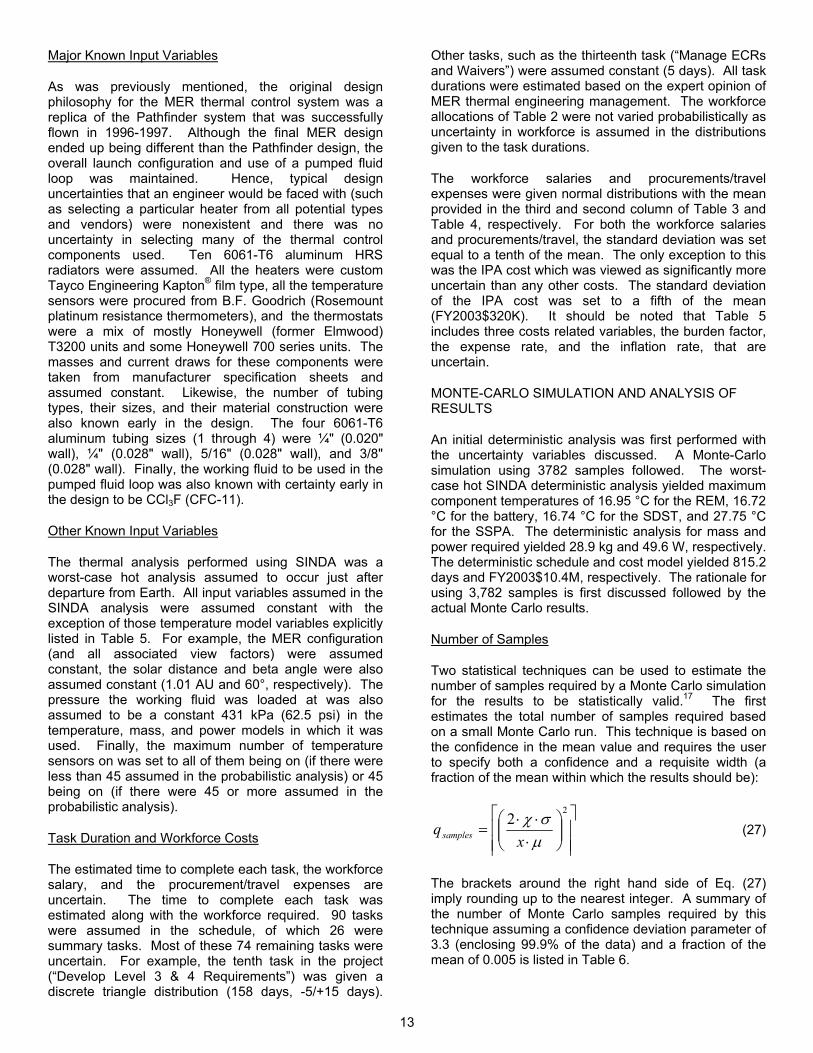
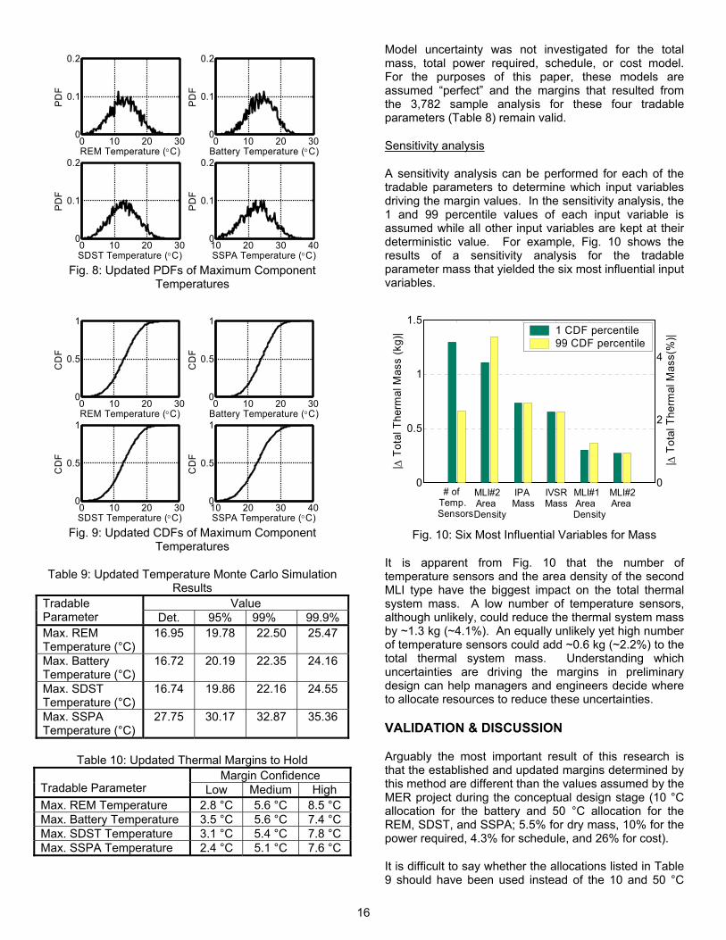
The updated PDFs of the four critical temperatures that include model uncertainty are shown in Fig. 8. The corresponding CDFs and statistical results corresponding to these updated results are shown in Fig. 9 and Table 9, respectively. Finally, based on the data in Table 9, the margins to hold can also be updated. These updated margins are shown in Table 10.

16

0 10 20 300

0.1

0.2

REM Temperature (°C)

PDF

0 10 20 300

0.1

0.2

Battery Temperature (°C)

PDF

0 10 20 300

0.1

0.2

SDST Temperature (°C)

PD

F

10 20 30 400

0.1

0.2

SSPA Temperature (°C)

PD

F

Fig. 8: Updated PDFs of Maximum Component

Temperatures

0 10 20 300

0.5

1

REM Temperature (°C)

CD

F

0 10 20 300

0.5

1

Battery Temperature (°C)

CD

F

0 10 20 300

0.5

1

SDST Temperature (°C)

CD

F

10 20 30 400

0.5

1

SSPA Temperature (°C)

CD

F

Fig. 9: Updated CDFs of Maximum Component

Temperatures

Table 9: Updated Temperature Monte Carlo Simulation Results

Value Tradable Parameter Det. 95% 99% 99.9% Max. REM Temperature (°C)

16.95 19.78 22.50 25.47

Max. Battery Temperature (°C)

16.72 20.19 22.35 24.16

Max. SDST Temperature (°C)

16.74 19.86 22.16 24.55

Max. SSPA Temperature (°C)

27.75 30.17 32.87 35.36

Table 10: Updated Thermal Margins to Hold Margin Confidence

Tradable Parameter Low Medium High Max. REM Temperature 2.8 °C 5.6 °C 8.5 °C Max. Battery Temperature 3.5 °C 5.6 °C 7.4 °C Max. SDST Temperature 3.1 °C 5.4 °C 7.8 °C Max. SSPA Temperature 2.4 °C 5.1 °C 7.6 °C

Model uncertainty was not investigated for the total mass, total power required, schedule, or cost model. For the purposes of this paper, these models are assumed “perfect” and the margins that resulted from the 3,782 sample analysis for these four tradable parameters (Table 8) remain valid.

Sensitivity analysis

A sensitivity analysis can be performed for each of the tradable parameters to determine which input variables driving the margin values. In the sensitivity analysis, the 1 and 99 percentile values of each input variable is assumed while all other input variables are kept at their deterministic value. For example, Fig. 10 shows the results of a sensitivity analysis for the tradable parameter mass that yielded the six most influential input variables.

0

0.5

1

1.5

| ∆ T

otal

The

rmal

Mas

s (k

g)|

0

2

4

| ∆ T

otal

The

rmal

Mas

s(%

)|1 CDF percentile99 CDF percentile

# of Temp. Sensors

MLI#2 Area Density

IPA Mass

IVSRMass

MLI#1 Area Density

MLI#2Area

Fig. 10: Six Most Influential Variables for Mass

It is apparent from Fig. 10 that the number of temperature sensors and the area density of the second MLI type have the biggest impact on the total thermal system mass. A low number of temperature sensors, although unlikely, could reduce the thermal system mass by ~1.3 kg (~4.1%). An equally unlikely yet high number of temperature sensors could add ~0.6 kg (~2.2%) to the total thermal system mass. Understanding which uncertainties are driving the margins in preliminary design can help managers and engineers decide where to allocate resources to reduce these uncertainties.

VALIDATION & DISCUSSION

Arguably the most important result of this research is that the established and updated margins determined by this method are different than the values assumed by the MER project during the conceptual design stage (10 °C allocation for the battery and 50 °C allocation for the REM, SDST, and SSPA; 5.5% for dry mass, 10% for the power required, 4.3% for schedule, and 26% for cost).

It is difficult to say whether the allocations listed in Table 9 should have been used instead of the 10 and 50 °C

17

allocation assumed. This is because only a small number of the variables assumed in the component maximum temperature analysis were treated as uncertain quantities, the vast majority were assumed to be known (deterministic). Some of these variables were indeed known and not uncertain; others were treated as known quantities to make the analysis tractable for the purpose of this research. Without doing a sensitivity analysis of all the variables in this temperature analysis it is not possible to quantitatively conclude that the allocations of Table 9 are correct.

The situation for the mass, power required, schedule, and cost margins is somewhat different. Although close to all (if not all) the uncertainties were taken into account in these four analyses, the model uncertainty was not. Although the authors believe these models to be satisfactory, there is certainly some model uncertainty associated with each. Verifying each of these models with actual data would result in the creation of model uncertainty distributions.

It should also be noted that other uncertainties that were discussed in the Introduction (such as ambiguity or volitional uncertainty) were not included in any of the five analyses. Nonetheless, the method presented in this paper and applied to the Mars Exploration Rover (MER) cruise stage thermal control system allows margins and allocations to be quantitatively determined based on the given design and uncertainties, not based on a historical number that is applied to all space systems. The method could be repeated and applied to the rover on the surface of Mars to determine the uncertainty and allocation to hold for the minimum temperature of the four critical components. Likewise, the analysis could be repeated at the critical design review (CDR) or beyond to update margins as the uncertainties in the design and development would have changed. The real benefit of this method is in the conceptual design period, around the preliminary design review (PDR), in establishing allocations and margins.

Both MER missions successfully landed on Mars in January 2004. In turn, the thermal control systems that were operating on the cruise stage during the trip to Mars were also successful. Both thermal control systems were satisfactorily designed, developed, and assembled. With the mission complete (at least from the perspective of the cruise stage thermal control system) it is possible to compare actual MER values with both the values assumed by the MER project (Current Method) and the values generated in this paper (Proposed Method). This is shown in Table 11.

Neglected round-off errors, Table 11 illustrates that the maximum temperatures predicted by the current method are successful for three of the four components while the proposed method is successful for all four. The current method is unduly conservative by allocated an extra 17.5 to 30.4 °C where it is not needed and missing the allocation for the battery by 12.5 °C. This conservatism

can primarily be explained by the worst-case on top of worst-case on top of worst-case type analysis which is typical in the thermal control community. Stacking of several worst-case scenarios is highly improbable and unduly penalizes the entire spacecraft design. For the proposed method, the REM, battery, SDST, and SSPA temperatures came in at 94th, 100th, 94th, and 99th percentiles. The battery temperature, although a 100th percentile, is within the round-off error of the analysis software.

For the mass, the current method was again unduly conservative, allocating an additional 7 kg that never materialized. The proposed method was much more accurate, coming in at a 58th percentile value. Discuss power here when I hear back from Adrian Adamson. The current method was more successful in predicting the schedule and cost of the cruise stage thermal control system. The schedule came in slightly below the allocation, the cost slightly above. The proposed method faired less well although this can easily be explained. The proposed method predicted a schedule that could range from ~782 to ~850 days which not credible based on the 770 day MER project allocation. That is to say, the proposed method indicated zero chance that the MER thermal control system could be build it 770 days. The cost corresponding to this (unrealistic) schedule was also low. MER did in fact trade cost for schedule early in its development. The total time to complete the project was significantly reduced by allocating additional workforce to complete critical tasks. In fact, MER traded too much cost for schedule since it ended up delivering the system 21 work days earlier than required. The proposed method would have faired much better in its predictions if it could have included this schedule-cost trade by, say, having a schedule that could range from 730 to 800 days and a corresponding cost for that schedule. The proposed method allows this trade to easily be completed; the current method does not.

As demonstrated, uncertainties play a significant role early on in the design of a complex multidisciplinary system. Engineers often think that displaying and discussing uncertainties is displaying a lack of understanding.19 However, an understanding of the impact of uncertainty must be understood for successful design, development, and operations. The method outlined in this paper and validated by the example provides a path toward this understanding through probabilistic methods.

18

Table 11: Comparision of Current and Proposed Methods with Actual Values for MER Current Method Proposed Method (99% confidence)

Tradable Parameter Actual Value Predicted Margin Allocation Predicted Margin Allocation

Max. REM Temperature 19.6 °C n/a n/a 50 °C 17.0 °C 5.5 °C 22.5 °C Max. Battery Temperature 22.5 °C n/a n/a 10 °C 16.7 °C 5.7 °C 22.4 °C Max. SDST Temperature 19.6 °C n/a n/a 50 °C 16.7 °C 5.5 °C 22.2 °C Max. SSPA Temperature 32.5 °C n/a n/a 50 °C 27.8 °C 5.1 °C 32.9 °C Thermal Mass 29.1 kg 34.3 kg 1.9 kg 36.2 kg 28.9 kg 2.2 kg 31.1 kg Maximum Power Required TBD W 60.3 W 6.0 W 66.3 W 49.6 W 13.7 W 63.3 W Thermal Schedule 749 days 738 days 32 days 770 days 815 days 35 days 850 days Thermal System Cost $12.8M $9.9M $2.6M $12.5M $10.4M $1.4M $11.8M CONCLUSION

A method for propagating and mitigating the effect of uncertainty in conceptual-level design via probabilistic methods has been presented. The goal of this research is to develop a rigorous foundation for determining design margins in complex multidisciplinary systems. A result of this work is a redefinition of the concept of design margin. Here, margins are a function of risk tolerance and are measured relative to mean expected system performance, not variations in design parameters measured relative to worst-case expected values. The investigated method was applied to the design and development of the cruise stage thermal control system of the Mars Exploration Rover (MER) mission. For the thermal example presented, margins for maximum component temperature, total mass, maximum power required, schedule, and cost formed a set of tradable system-level parameters. Assuming a medium-confidence approach to design and development, the proposed method established margins that differed from margins that were assumed during conceptual design. Although the proposed method did not perform as well as the current method for the schedule and cost, differences in the proposed method with actual values were easily explained. Differences in the current method with actual values were typically on the side of conservatism and much more difficult to explain or revise. The proposed method demonstrates the benefits of using probabilistic methods to develop the entire distribution of uncertain parameters for decision making and not relying on extreme (worst-case) values.

ACKNOWLEDGEMENTS

This research is part of the Space Systems, Policy, and Architecture Research Consortium (SSPARC) funded by the National Reconnaissance Office (Chantilly, VA). The MER thermal design effort was carried out by the Jet Propulsion Laboratory, California Institute of Technology under a contract with the National Aeronautics and Sapce Administration. The authors thank Robert Krylo, Eric Sunada, Gani Ganapathi, Gaj Birur (Thermal and Propulsion Engineering Section, JPL, Pasadena, CA), Brent Cullimore (C&R Technologies, Inc., Littleton, CO), and John Welch (The Aerospace Corporation, El Segundo, CA) for their consultation and expertise.

REFERENCES 1Gilmore, D., Spacecraft Thermal Control Handbook, Aerospace Corp., El Segundo, CA, 2002, pp. 411-412, 534-537, 714-725. 2Thunnissen, D., “Uncertainty Classification for the Design and Development of Complex Systems,” Proceedings of the 3rd Annual Predictive Methods Conference, June, 2003. 3Stark, R., “Thermal Testing of Spacecraft,” The Aerospace Corporation, Report No. TOR-0172(2441-01)-4, El Segundo, CA, September 1971. 4Test Requirements for Launch, Upper-Stage, and Space Vehicles, Military Standard, MIL-STD-1540C, September 1994. 5Welch, J., “A Comparison of Satellite Flight Temperatures with Thermal Balance Test Data,” SAE Technical Paper 2003-01-2460, July 2003. 6Roncoli, R. and Ludwinski, J., “Mission Design Overview for the Mars Exploration Rover Mission,” AIAA Paper 2002-4823, August 2002. 7Birur, G. and Bhandari, P., “Mars Pathfinder Active Heat Rejection System: Successful Flight Demonstration of a Mechanically Pumped Cooling Loop,” SAE Technical Paper 981684, July 1998. 8Ganapathi, G., Birur, G., Tsuyuki, G., McGrath, P., and Patzold, J., “Active Heat Rejection System on Mars Exploration Rover – Design Changes from Mars Pathfinder,” Proceedings of the Space Technology and Applications International Forum (STAIF), Institute for Space and Nuclear Power Studies, Albuquerque, NM, 2003, pp. 206-217. 9Tsuyuki, G., Ganapathi, G., Bame, D., Patzold, J., Fisher, R., and Theriault, L., “The Hardware Challenges for the Mars Exploration Rover Heat Rejection System,” Proceedings of the Space Technology and Applications International Forum (STAIF), Institute for Space and Nuclear Power Studies, Albuquerque, NM, 2004, pp. 59-70. 10Cullimore, B., Ring, S., and Johnson, D., SINDA/FLUINT User’s Manual, C&R Technologies, Inc., Revision 17, Littleton, CO, September 2003. 11Platzer, B., Polt, A., and Maurer, G., “Refrigerant R11 (CCl3F),” Thermophysical Properties of Refrigerants, Springer-Verlag, Berlin, Germany, 1990, pp. 30-32. 12Thunnissen, D. and Nakazono, B., “Propagating and Mitigating the Effect of Uncertainty in the Conceptual

19

Design of a Monopropellant Propulsion System,” AIAA Paper 2003-4469, July 2003. 13“Thermophysical Properties of Refrigerants,” 1997 ASHRAE Handbook: Fundamentals: SI Edition, American Society of Heating, Refrigerating and Air-Conditioning Engineers (ASHRAE), Atlanta, GA, 1997, p. 19-3. 14White, F., “The Circular Pipe: Hagen-Poiseuille Flow,” Viscous Fluid Flow, 2nd edition, McGraw-Hill, Inc., New York, NY, 1991, p. 117. 15Sabersky, A., Acosta, A., Hauptmann, E., and Gates, E., Fluid Flow: A First Course in Fluid Mechanics, 4th edition, Prentice Hall, Upper Saddle River, NJ, 1999, pp. 187-192. 16Lindeburg, M., “Hydraulic Machines,” Mechanical Engineering Reference Manual for the PE Exam, 11th edition, Professional Publications, Inc., Belmont, CA, 2001, p. 18-7, 18-8. 17Morgan, M. and Henrion, M., “Monte Carlo and Other Sampling Methods,” Uncertainty: A Guide to Dealing with Uncertainty in Quantitative Risk and Policy Analysis, Cambridge University Press, Cambridge, United Kingdom, 1990, pp. 198-203. 18Thunnissen, D., Engelbrecht, C., and Weiss, J., “Assessing Model Uncertainty in the Conceptual Design of a Monopropellant Propulsion System,” AIAA Paper 2003-4470, July 2003. 19Seife, C., “Columbia Disaster Underscores the Risky Nature of Risk Analysis,” Science, Vol. 299, February 14, 2003, p. 1001.

DEFINITIONS

A cross-sectional area, m2

A, B beta distribution parameters

a, b, c viscosity coefficients

B mass flow rate, kg/sec

E voltage, V

f friction factor

G volume flow rate, m3/sec

I current, A

k conical loss coefficient

l length, m

l/φ equivalent length over diameter

m mass, kg

n total number of tubing sections

n, p binomial distribution parameters

Q heat rejected, W

q total quantity of an item

P power required, W

Px xth percentile value

p pressure, Pa, or percentile

Rdet deterministic result value

S surface area, m2

T temperature, K

t thickness, m

V volume, m3

v flow rate, m/sec

x fraction

z total number of MLI types

α absorptivity

∆p pressure drop, Pa, or percentile

ε emissivity

ζ area density, kg/m2

η efficiency

κ burden factor

µ viscosity, kg/m-sec, or mean

ρ density, kg/m3

σ standard deviation

φ diameter, m

χ confidence deviation difference

ψ percent value

subscripts

b&f brackets & fittings

con contraction

20

elb_bends elbow bends

exp expansion

exp_rate expense rate

fluid working fluid

HRS heat rejection system

HRS_rad HRS radiator

inf_rate inflation rate

IPA integrated pump assembly

IVSR IPA, vent, shunt limiter, and radiator

misc total miscellaneous components

MLI multilayer insulation

op operating

REM rover electronics module

ret_bends return bends

SDST small deep space transponder

shunt_rad shunt radiator

SSPA solid state power amplifier

φ diameter

φ_change diameter change

superscripts

j tubing section number

k MLI type number

CONTACT INFORMATION

M/C: 205-45 1200 East California Boulevard Pasadena, California 91125-4500 dthunnis@its.caltech.edu (626) 395-4785