margin-based asset pricing and deviations from the law...

Margin-based Asset Pricing and Deviationsfrom the Law of One Price

Nicolae GarleanuUniversity of California

Lasse Heje PedersenNew York University

In a model with heterogeneous-risk-aversion agents facing margin constraints, we showhow securities’ required returns increase in both their betas and their margin require-ments. Negative shocks to fundamentals make margin constraints bind, lowering risk-freerates and raising Sharpe ratios of risky securities, especially for high-margin securities.Such a funding-liquidity crisis gives rise to “bases,” that is, price gaps between securitieswith identical cash-flows but different margins. In the time series, bases depend on theshadow cost of capital, which can be captured through the interest-rate spread betweencollateralized and uncollateralized loans and, in the cross-section, they depend on rela-tive margins. We test the model empirically using the credit default swap–bond bases andother deviations from the Law of One Price, and use it to evaluate central banks’ lendingfacilities. (JEL G01, G12, G13, E44, E50)

The paramount role of funding constraints becomes particularly salient dur-ing liquidity crises, with the one that started in 2007 being an excellent casein point. Banks unable to fund their operations closed down, and the fund-ing problems spread to other investors, such as hedge funds, that relied onbank funding. Therefore, traditional liquidity providers became forced sellers,interest-rate spreads increased dramatically, Treasury rates dropped sharply,and central banks stretched their balance sheets to facilitate funding. Thesefunding problems had significant asset-pricing effects, the most extreme exam-ple being the failure of the Law of One Price (LoOP): Securities with (nearly)

We are grateful for helpful comments from Markus Brunnermeier, Xavier Gabaix, Andrei Shleifer, and WeiXiong, as well as from seminar participants at the Bank of Canada, Columbia GSB, Duke Fuqua, Harvard,London School of Economics, MIT Sloan, McGill University, Northwestern University Kellog, UT Austin Mc-Combs, Yale University, UC Berkeley Haas, University of Chicago, and McGill University, as well as conferenceparticipants at the Yale Financial Crisis Conference, the Society of Economic Dynamics, NBER Behavioral Eco-nomics, NBER Asset Pricing Summer Institute, NASDAQ OMX Derivatives Research Project Conference, theEconometric Society Winter Meeting, and the Western Finance Association Meetings. Send correspondence toNicolae Garleanu, Haas School of Business, University of California, Berkeley, NBER, and CEPR; telephone:(510) 642-3421. E-mail: [email protected]. Pedersen is at New York University, CEPR, NBER, andAQR Capital Management, 44 West Fourth Street, NY 10012-1126. E-mail: [email protected], http://www.stern.nyu.edu/∼lpederse/.

c© The Author 2011. Published by Oxford University Press on behalf of The Society for Financial Studies.All rights reserved. For Permissions, please e-mail: [email protected]:10.1093/rfs/hhr027 Advance Access publication April 14, 2011

Margin-based Asset Pricing and Deviations from the Law of One Price

identical cash flows traded at different prices, giving rise to so-called “bases”(i.e., price gaps).

We attempt to explain these effects using a dynamic general-equilibriummodel with realistic margin constraints, and to test empirically the model’stime-series and cross-sectional predictions of how funding problems affect riskand return.

Our model shows that (i) the consumption capital asset-pricing model(CCAPM) is augmented by a security’s margin times the general funding cost;(ii) a basis between a security and a derivative with identical cash flows arisesas the difference in their margin requirements times the funding cost, plustheir endogenous difference in beta; (iii) securities with higher margins havelarger betas and volatilities during crises, since they have larger funding liquid-ity risk; (iv) the funding cost can be captured by the interest-rate differentialbetween collateralized and uncollateralized borrowing; (v) the margin effectstrengthens nonlinearly in “bad times” as margin requirements are hit, leadingto sharp drops in the risk-free collateralized and Treasury rates, to a rise in thespread between collateralized and uncollateralized interest rates, and to a risein risk premia and especially margin premia. We also (vi) calculate the equi-librium and calibrate the magnitude and dynamics of the bases using macroparameters.

In our applications, we (vii) find statistically significant empirical evidenceconsistent with the model’s predictions for the time series of the credit defaultswap (CDS)–bond basis, for the cross-sectional difference between investment-grade and high-yield bases, and for the levels and time variation of CDS andbonds risks; (viii) find consistent evidence from the failure of the coveredinterest-rate parity; (ix) compute the asset-pricing effect of the Fed’s lendingfacilities; and (x) quantify a bank’s incentive to perform regulatory arbitrageto loosen capital requirements.

Our model considers a group of (relatively) risk-averse agents and a groupof (relatively) risk-tolerant agents. Each risk-tolerant investor uses leverage,but is subject to margin requirements. He must fund all the margins on hispositions with his equity capital and, possibly, uncollateralized loans. Onecan think of these leveraged investors as banks or the financial sector morebroadly, including hedge funds. The risk-averse investors may be constrainedin their trading of derivatives and cannot lend uncollateralized, so the un-collateralized loan market is a pure “inter-bank market” for the risk-tolerantinvestors.

We first show how margin requirements affect the required returns for bothunderlying assets and derivatives.1 For a typical asset in which the risk-tolerant

1 If there were no redundant securities and margins were constant over time, the result for the underlying assetswould specialize a result fromCuoco(1997) for general convex portfolio constraints, and it is also closely relatedto results fromAiyagari and Gertler(1999) andHindy and Huang(1995).

1981

The Review of Financial Studies / v 24 n 6 2011

agents hold long positions in equilibrium, the required excess returnE(r i ) is

E(r i )= r risk-free + β i × covariance risk premium

+ mi × margin premium, (1)

wheremi is the margin requirement (and all quantities may be time varying).The first two terms in this “margin CAPM” are the same as in the standard(consumption) CAPM, namely, the risk-free interest rate and the covariancerisk premium. Hence, if the margin requirements are zero, our model natu-rally nests the standard model. With positive margin requirements—as in thereal world—the higher a security’s margin requirement, the higher its requiredreturns. The margin premium is the shadow cost of funding for the risk-tolerantagents multiplied by the relative importance of these agents. Consequently, itis positive when margin constraints are binding, and zero otherwise. For in-stance, supposing that in a crisis the risk-tolerant investors have a shadow costof capital of 10% (consistent with our estimates during the height of the GlobalFinancial Crisis and with our calibration) and the risk-tolerant investors ac-count for 40% of the aggregate risk tolerance, the margin premium is 4%.Therefore, if a security has a margin requirement of 50%, then its requiredreturn is 4%× 50% = 2% higher than the level predicted by the standardCCAPM, a significant effect.

Our model suggests that constrained investors would evaluate securitiesbased on a ratio that we callalpha per margin(AM):

AMi =E(r i )− r risk-free− β i × covariance riskpremium

mi. (2)

This is the abnormal return (in excess of the risk-free rate and the standardrisk adjustment) on a strategy of investing a maximally leveraged dollar in theasset. Hence, the margin CAPM in (1) can be stated equivalently by sayingthat, in equilibrium, all assets have the same AM,AMi = margin premium.While, in the classical CAPM, alpha is zero for all assets, in our model, alphascan be non-zero when capital constraints bind, and AM ratios are equalized asinvestors seek to maximize their leveraged return.

We show that “bad times” with binding margin constraints naturally occurafter negative shocks to fundamentals. This phenomenon leads to several in-triguing effects. First, risk-free interest rates for collateralized loans and Trea-suries spike down. This happens because the risk-tolerant agents cannot borrowas much as they would like due to margin constraints and, therefore, in equilib-rium the risk-averse agents must lend less than they otherwise would. In orderto induce the risk-averse agents not to lend, the interest rate must drop.

Further, in bad times the spread between the interbank uncollateralized loansand the collateralized loans (or Treasuries) increases, even abstracting fromcredit risk. This liquidity-driven interest-rate premium arises from the fact thatthe risk-averse investors do not participate in the uncollateralized inter-bank

1982


market. Since the risk-tolerant banks are constrained, the inter-bank interestrate must be greater than the Treasury rate to reflect the banks’ positive shadowcost of capital. While this pure liquidity-driven interest-rate spread is zero in“normal” times when margin requirements do not bind, it increases nonlinearlyfollowing negative shocks as when the crisis hit in 2007, as well as in previousliquidity crises.

Hence, the deviation from the standard CAPM is most apparent in bad times,when the funding-liquidity effects are the strongest. A stark illustration ofthis margin-based asset-pricing effect is the price difference between secu-rities with the same cash flows but different margin requirements. We showthat the required return on a high-margin security—e.g., a corporate bond—isgreater than that of a low-margin security with the same cash flows—e.g., prox-ied by a CDS. This is because of the high shadow cost of capital of the risk-tolerant investor. When the risk-tolerant investor’s margin constraint binds, heis willing to accept a lower yield spread on a CDS, since it uses less margincapital.

As empirical evidence of this prediction, we find that the time-series vari-ation of the CDS-bond basis has a statistically significant co-movement withthe LIBOR–general collateral (GC) repo interest-rate spread (i.e., the spreadbetween uncollateralized and collateralized loans), as well as the tightness ofcredit standards as estimated by the Federal Reserve Board’s “Senior LoanOfficer Opinion Survey on Bank Lending Practices.”

The model predicts that the magnitude of the basis is the shadow cost ofcapital times the margin difference plus the difference in betas. To understandthis predicted magnitude, consider the CDS–bond basis, that is, the yield dif-ference between a corporate bond and a comparable derivative. With a shadowcost of capital of 10% during the crisis, a margin on investment-grade bondsof 25%, and a margin on the corresponding CDS of 5%, the direct effect ofthe margin difference on the basis is 10%× (25%− 5%) = 2%, close to whatwas observed empirically. Additionally, the model predicts that the corporatebond’s higher margin makes it riskier, since it is more sensitive to further fund-ing crises, leading to an additional, albeit smaller, effect on the basis.

When there are several pairs of underlying/derivative securities, each ofwhich has an associated basis, our model predicts that these bases are cor-related in the time series due to their common dependence on the shadow costof capital and, cross-sectionally, the bases should be proportional to each pair’sdifference in margin requirements.

To test these cross-sectional predictions empirically, we compare the basisof investment-grade (IG) bonds with the basis for high-yield (HY) bonds andfind that they move closely together and that the difference in their magnitudescorresponds to the difference in their margins, consistent with our model’sprediction. Indeed, the margin difference between HY bonds and CDS is abouttwice that of IG bonds/CDS, so the model predicts an HY basis that is abouttwice the IG basis, consistent with the data.

1983


Interestingly, the model also implies that securities with identical cash flowsbut different margins have different risk characteristics due to their differentexposures to funding-liquidity risk. The low-margin CDS has less systematicrisk since its price drops less in liquidity crisis and, therefore, its requiredreturn is lower even before the margin constraint binds. Consistent with themodel, we find empirically that bonds and CDSs have similar betas and volatil-ities during “normal” times when constraints are not near binding, but that be-tas and volatilities of high-margin bonds rose above those of CDSs during the2007–2009 liquidity crisis.

Further consistent evidence arises from the related time-series variation ofthe interest-rate spread and that of the deviation from the covered interest par-ity (CIP). Indeed, during the funding crises of 1998 and 2007–2009, whenmargins are likely to have been binding, interest-rate spreads were wide andthe CIP deviation was substantial, since agents did not have enough capital toeliminate it.

As another application of the model, we show how the Fed’s lending facili-ties affect asset prices, providing new insights into the monetary transmissionmechanism during liquidity. We discuss how the lending facilities lower mar-gin requirements, and show that the model-implied increase in asset prices is ofthe same order of magnitude as the increase attributable to lowered margins inthe banks’ bid prices, according to surveys conducted by the Federal ReserveBank of New York.

Further, we derive the shadow cost of banks’ regulatory-capital require-ments, which gives an estimate of their incentive to perform regulatory ar-bitrage by placing assets off the balance sheet or tilting toward AAA securitieswith low capital requirements.

This article is related to a number of strands of literature. Borrowing con-straints confer assets a collateral value (Bernanke and Gertler 1989; Hindy1995; Detemple and Murthy 1997; Geanakoplos 1997; Kiyotaki and Moore1997; Caballero and Krishnamurthy 2001; Lustig and Van Nieuwerburgh 2005;Coen-Pirani 2005; Fostel and Geanakoplos 2008), and constraints open thepossibility of arbitrage in equilibrium (Basak and Croitoru 2000, 2006;Geanakoplos 2003). We focus on margin requirements, which are linked tomarket liquidity and volatility (Gromb and Vayanos 2002; Brunnermeier andPedersen 2009; Adrian and Shin 2010; Danielsson, Shin, and Zigrand 2009;Rytchkov 2009), and provide analytic asset-pricing effects. Asset prices alsodepend on market liquidity (Amihud and Mendelson 1986; Longstaff 2004;Duffie, Garleanu, and Pedersen 2007; Garleanu, Pedersen, and Poteshman2009), market liquidity risk (Acharya and Pedersen 2005; Mitchell, Pedersen,and Pulvino 2007; He and Krishnamurthy 2008), limits to arbitrage (Shleiferand Vishny 1997), banking frictions (Allen and Gale 1998, 2004, 2005;Acharya and Viswanathan 2011), and related corporate-finance issues(Holmstrom and Tirole 1998, 2001). We use the methods for analyzing equilib-ria in continuous-time models with constraints ofCuoco (1997); other

1984


related applications are provided byLi (2008), Rytchkov(2009), Chabakauri(2010), andPrieto(2010).2

The specification of the margin requirement is key to our results. First, wemake the realistic assumption that both long and short positions use capi-tal; in contrast, a linear constraint, as often assumed in the literature, impliesthat shorting frees up capital. While bases with natural properties arise in ourmodel, we show that no basis can obtain in a world in which all agents faceonly the same linear constraint. Second, we consider assets with identical cashflows and different margin requirements, while margins for such assets wouldbe the same if margins arose solely from limited commitment (Geanakoplos1997). In the real world, securities with (almost) identical cash flows can havesubstantially different margins, since margins depend on the market liquidityof the securities (Brunnermeier and Pedersen 2009) and because of variousinstitutional frictions. For instance, corporate bonds have low market liquid-ity in over-the-counter search markets (Duffie, Garleanu, and Pedersen 2005,2007;Vayanos and Weill 2008), and this makes them less attractive as collat-eral because they can be difficult to sell. Further, to get credit exposure througha corporate bond, one must actually buy the bond for cash and try to fund itusing a repo, which uses a broker’s balance sheet, while a CDS is an “un-funded” derivative with zero net present value, so the margin is necessary onlyto limit counterparty risk; the CDS does not inherently use cash. Our modelfurther allows for time-varying margins, given that margins tend to increaseduring crises due to a margin spiral, as explained byBrunnermeier andPedersen(2009) and documented empirically byGorton and Metrick(2009).

We complement the literature by providing a tractable model with explicitpricing equations that provide testable time-series and cross-sectional implica-tions, deriving the basis (i.e., price gap) between securities with identical cashflows depending on their different margins, showing how the shadow cost offunding can be captured using interest-rate spreads, calibrating the magnitudeand dynamics of the predicted deviations from the LoOP using realistic param-eters, testing the theory empirically using the CDS–bond basis and the failureof the CIP, and applying the theory to the Federal Reserve’s lending facilitiesand the incentive to perform regulatory arbitrage.

The rest of the article is organized as follows. Section1 lays out the model,Section2 derives our main theoretical results and calibrates the model, andSection3 applies the model empirically to the CDS–bond basis, the failure ofthe covered interest-rate parity, and the pricing of the Fed’s lending facilities,and quantifies the cost of banks’ regulatory capital requirements. Section4concludes.

2 Numerous papers study frictionless heterogeneous-agent economies, e.g.,Dumas(1989), Wang(1996), Chanand Kogan(2002), Bhamra and Uppal(2009), Weinbaum(2009), Garleanu and Panageas(2008), andLongstaffand Wang(2009).

1985


1. Model

We consider a continuous-time economy in which several risky assets aretraded. Each asseti pays a dividendδi

t at time t and is available in a supplynormalized to 1. The dividend of each securityi is a continuous Ito processdriven by a multidimensional standard Brownian motionw:3

dδit = δi

t

(μδ

i

t dt + σ δi

t dwt

), (3)

whereμδi

t is the dividend growth, and the dividend volatility is given by the

vectorσ δi

t of loadings on the Brownian motion.Each security is further characterized by its margin (also called a haircut)

mit ∈ [0, 1], an Ito process, measured as a fraction of the investment that must

be financed by an agent’s own capital, as discussed below. For instance, themargin on a corporate bond could bembond

t = 50%, meaning that an agent canborrow half of the value and must pay the other half using his own capital.

In addition to these “underlying assets” in positive supply, the economy hasa number of “derivatives” in zero net supply. Each derivativei ′ has the samecash flowsδi

t as some underlying securityi , but with a lower margin require-ment:mi ′

t < mit .

We assume that the prices of underlying assets and derivatives are Ito pro-cesses with expected return (including dividends) denotedμi

t and volatilityvectorsσ i

t , which are linearly independent across the underlying assets:

d Pit = (μi

t Pit − δi

t )dt + Pit σ

it dwt . (4)

Finally, the set of securities includes two riskless money-market assets, onefor collateralized loans and one for uncollateralized loans, as explained fur-ther below. The equilibrium interest rate for collateralized loans isr c

t , and foruncollateralized loans isr u

t .The economy is populated by two agents: Agenta is averse to risk, whereas

b isbraver. Specifically, agentg ∈ {a, b} maximizes his utility for consumptiongiven by

Et

∫ ∞

0e−ρsug(Cs) ds, (5)

whereua(C) = 11−γ a C1−γ a

with relative risk aversionγ a > 1, andub(C) =

log(C) with relative risk aversionγ b = 1. We can think of agenta as a rep-resentative pension fund or risk-averse private (retail) investor, and of agentb

3 All random variables are defined on a probability space(Ω,F) and all processes are measurable with respect tothe augmented filtrationFwt generated byw.

1986


as representing more risk-tolerant investors using leverage, such as banks orhedge funds.

At any timet , each agentg ∈ {a, b} must choose his consumption,Cgt (we

omit the superscriptg when there is little risk of confusion), the proportionθ i

t of his wealthWt that he invests in risky asseti , and the proportionηut in-

vested in the uncollateralized loans; the rest is invested in collateralized loans.The agent must keep his wealth positive,Wt ≥ 0, and the wealth evolvesaccording to

dWt =

(

Wt

(

r ct + ηu

t (rut − r c

t )+∑

i

θ it (μ

it − r c

t )

)

− Ct

)

dt

+ Wt

∑

i

θ it σ

it dwt , (6)

where the summation is done over all risky underlying and derivativesecurities.

Each agent faces a margin constraint that depends on the securities’marginsmi

t :

∑

i

mit |θ

i | + ηu ≤ 1. (7)

In words, an agent can tie up his capital in margin for long or short positionsin risky assets and invest in uncollateralized loans (or borrow uncollateralizedif ηu < 0), and these capital uses, measured in proportion of wealth, must beless than 100% of the wealth. The rest of the wealth, as well as the money inmargin accounts, earns the collateralized interest rate.4 This key constraint isa main driver of our results. The literature often assumes a linear margin con-straint (i.e., without the absolute-value operator), but AppendixA shows thatdeviations from the LoOP cannot arise in this case. Our constraint captureswell the problem facing any real-world investor (e.g., real-world investors can-not finance unlimited long positions by short ones, as is implied by the linear

4 Alternatively, the constraint can be written as

∑

i

|θ i | + ηu ≤ 1 +∑

i

|θ i |l i .

For a long position,l i is the proportion of the security value that can be borrowed in the collateralized lendingmarket (e.g., the repo market). Hence, the left-hand side of the equation is the fraction of wealthθ i used to buythe security, and the right-hand side is the total wealth 1 plus the borrowed amountθ i l i . Naturally, the marginmi = 1 − l i is the fraction of the security value that cannot be borrowed against.

For a short position, one must first borrow the security and post cash collateral of(1 + mi )θ i and, since theshort sale raisesθ i , the net capital use ismi θ i . Derivatives with zero net present value have margin requirements,too. SeeBrunnermeier and Pedersen(2009) for details.

1987


constraint), and it gives rise to deviations from the LoOP that match thoseobserved empirically.

In addition, the risk-averse agenta does not participate in the markets for un-collateralized loans and may be allowed only limited positions in derivatives.That is, he must chooseηu = 0 andθ i ′ ∈ Ai ′ for every derivativei ′, where theadmissible setAi ′ can, for instance, be specified asAi ′ = {0}, meaning that hecannot trade derivatives, or asAi ′ = [A,A], meaning that he can trade only alimited amount. This captures the fact that certain agents are often limited byrisk aversion, by a lack of willingness to participate in some transactions, e.g.,those with apparent operational risk—i.e., the risk that something unspecifiedcan go wrong—and by a lack of expertise. Also, this means that the uncollat-eralized market may capture an interbank loan market.

Our notion of equilibrium is standard. It is a collection of prices, consump-tion plans, and positions such that (i) each agent maximizes his utility giventhe prices and subject to his investment constraints; and (ii) the markets forrisky and risk-free assets clear.

2. Margin-based Asset Prices

We are interested in the properties of the equilibrium and consider first theoptimization problem of the brave agentb using dynamic programming. Thelogarithmic utility for consumption implies that the Hamilton–Jacobi–Bellman(HJB) equation reduces to the myopic mean-variance maximization

maxθ i

t ,ηut

{r ct + ηu

t

(r ut − r c

t

)+∑

i

θ it (μ

it − r c

t )−1

2

∑

i, j

θ it θ

jt σ

it (σ

jt )

>}, (8)

subject to the margin constraints∑

i mit |θ

it | + ηu

t ≤ 1.Attaching a Lagrange multiplierψ to the margin constraint, the first-order

condition with respect to the uncollateralized investment or loanηu yields thefollowing result.

Proposition 1 (Interest-Rate Spread). The interest-rate differential betweenuncollateralized and collateralized loans captures the risk-tolerant agent’sshadow cost of an extra dollar of funding,r u

t − r ct = ψt .

The proposition identifies the shadow cost of capital, central to our asset-pricing analysis, as the interest-rate differential between uncollateralized loans,which do not use up a borrower’s potentially scarce collateral, and collateral-ized loans, which do. In addition to having intuitive appeal, this relationship isvaluable for linking the unobserved shadow cost of capitalψ to quantities inprinciple observable; we use it in our empirical analysis.

1988


Agentb’s first-order condition with respect to the risky-asset positionθ i is

μit − r c

t = βCb,it + ψtmi

t if θ i > 0

μit − r c

t = βCb,it − ψtmi

t if θ i < 0

μit − r c

t = βCb,it + yi

tψtmit with yi

t ∈ [−1, 1] if θ i = 0,

(9)

where we simplify notation by letting

βCb,it = covt

(dCb

Cb,

d Pi

Pi

)(10)

denote the conditional covariance between agentb’s consumption growth andthe return on securityi . These first-order conditions mean that a security’sexpected excess returnμi

t − r ct depends on its marginmi

t , the risk-tolerantagent’s shadow cost of fundingψt , and the security’s covariance with the risk-tolerant agent’s consumption growth.

To characterize the way in which returns depend on aggregate consumption(which is easier to observe empirically), we also need to consider agenta’soptimal policy and aggregate across agents.5 If a’s margin requirement doesnot bind, standard arguments show that the underlying securities are priced byhis consumption,μi − r c = γ aβCa,i , but the general problem with marginconstraints and spanned securities is more complex. In the general case, wederive a consumption CAPM depending on aggregate consumption in the ap-pendix. For this, we first introduce some notation:βC,i

t is the covariance of thegrowth in the aggregate consumptionC = Ca + Cb and the return of securityi ,

βC,it = covt

(dC

C,

d Pi

Pi

), (11)

andγt is the “representative” agent’s risk aversion, i.e.,

1

γt=

1

γ a

Cat

Cat + Cb

t+

1

γ b

Cbt

Cat + Cb

t. (12)

The fractionxt of the economy’s risk-bearing capacity due to agentb is

xt =

Cbtγ b

Catγ a + Cb

tγ b

. (13)

We recall thatψ is agentb’s shadow cost of funding. With these definitions, weare ready to state the margin-adjusted CCAPM and CAPM. For simplicity, we

5 See Proposition 3 inCuoco(1997) for a CAPM relation for general time-invariant convex portfolio constraintsin the absence of redundant securities.

1989


do it under the natural assumption that the margin constraint of the risk-averseagenta does not bind.6

Proposition 2 (Margin CCAPM). The expected excess returnμit − r c

t onan underlying asset that agentb is long is given by the standard consumptionCAPM adjusted for funding costs:

μit − r c

t = γtβC,it + xtψt mi

t. (14)

If agentb is short the asset, then the funding-liquidity term is negative, i.e.,μi

t − r ct = γtβ

C,it − xtψt mi

t , while if b has a zero position, the required returnlies between the two values.

This proposition relates excess returns to the covariance between aggregateconsumption growth and a security’s returns, as well as to the funding con-straints. The covariance term is the same as in the classic CCAPM model ofBreeden(1979). The difference is the funding term, which is the product of thesecurity-specific marginmi

t and the general coefficientsψt andxt that measurethe tightness of the margin constraints. Naturally, the tightness of the marginconstraint depends on the leveraged risk-tolerant agent’s shadow cost of fund-ing,ψ , and the relative importance of this agent,x.

The margin CCAPM’s economic foundation dictates the magnitude of thecoefficients. Sinceγ b = 1 andγ a is a number between 1 and 10, say, theaggregate risk aversionγt is somewhere between 1 and 10, and varies overtime depending on the agents’ relative wealths. The relative importancex ofagentb is a number between 0 and 1. While this risk-tolerant agent might bea small part of the economy in terms of total consumption or wealth, his risktolerance is larger, which raises his importance. For instance, even if we thinkthat he accounts for only as little as 2% of the aggregate consumption, andif agenta has a risk aversion of 10, thenx is around 17%, close to 10 timesthe consumption share. The shadow costψ can be as much as 10% in ourcalibration and empirical analysis. Hence, for a security with a 50% margin,the funding term would raise the required return by 17%× 10%× 50%≈ 1%in this case.

For a different way to interpret the relationship in Equation (14), considerthe “alpha” of asseti , that is, the expected excess return adjusted for risk,αi

t = μit − r c

t − γtβC,it . The margin CCAPM says that alphas are proportional

to margin requirements,ψxtmit , or, in terms of the ratioalpha per margin

(AM), it says thatAMi is constant across securitiesi ,

AMit = xtψt .

6 We state and prove the propositions without this assumption in the appendix, but focus on this case because it isnatural and simpler to state and obtains in our calibrated equilibrium in Section2.1. In the general case, Equation(B.1) contains the additional term that capturesa’s margin constraint,+(1− xt )ψt , whereψt is a’s shadow costof capital, and similarly for Equation (16).

1990


For instance, if a security has a margin requirement of 10%, it can be leveraged10 to 1. In this case,AMi = 10× α must equal the aggregate shadow cost ofcapitalxtψt to make it worthwhile for the agents to use margin equity to holdthis security.

The CAPM can also be written in terms of a mimicking portfolio in place ofthe aggregate consumption. Specifically, letq be the portfolio whose return hasthe highest possible (instantaneous) correlation with aggregate consumptiongrowth andqi

t be the weight of asseti in this portfolio. Further, the return betaof any asseti to portfolioq is denoted byβ i

t , i.e.,

β it =

covt

(d Pq

Pq ,d Pi

Pi

)

vart(d Pq

Pq

) . (15)

Proposition 3 (Margin CAPM). Suppose that the margin constraint of agenta does not bind. The expected excess returnμi

t −r ct on an underlying asset that

b is long is

μit − r c

t = λtβit + xtψt mi

t , (16)

whereλt is a covariance risk premium. Ifb is short, then the margin term isnegative, i.e.,μi

t − r ct = λtβ

it − xtψt mi

t , and otherwise the required return liesbetween the two values.

We next turn to the basis between underlying securities and derivatives. Theoptimization problem of the brave agentb implies the following relation forthe basis.

Proposition 4 (Basis). A basis arises whenb’s margin constraint binds anda’s derivative-trading constraint or margin constraint binds. Depending on theconstraints, the basis is influenced by the difference or sum of margins:

(A. Levered Investor Causing Basis)Suppose that agentb is long securityi and long derivativei ′. Then the required return spreadμi

t − μi ′t between

securityi and derivativei ′ (the “basis”) depends on the shadow cost of capitalψ , the securities’ difference in margins,mi

t − mi ′t , and the difference in their

covariance with the consumption of the brave agentb through

μit − μi ′

t =ψt

(mi

t − mi ′t

)+(βCb,i

t − βCb,i ′t

). (17)

(B. Levered Investor Reducing Basis)If agentb is longi and short derivativei ′, then the basis equals

μit − μi ′

t =ψt

(mi

t + mi ′t

)+(βCb,i

t − βCb,i ′t

). (18)

1991


This proposition provides useful intuition about the drivers of a basis. Sincea non-zero basis constitutes a failure of the LoOP, all agents must be con-strained for this to happen in equilibrium. Such a situation obtains when therisk-tolerant agentb is constrained by his leverage and agenta is constrainedby his limited ability to hold derivatives.

If the risk-averse investor can short only a limited amount of derivatives,then case A in the proposition arises. In this case, the risk-tolerant investorbwants to go long both the underlying and the derivative to earn the associatedrisk premium. He can get exposure to the derivative with less use of marginand, therefore, he is willing to accept a smaller return premium on the deriva-tive. In fact, the basis as measured by the return spread is thedifferencein mar-gins multiplied by the shadow cost of capital, adjusted for the beta difference.

The second case obtains, for instance, if agenta has a structural need—for some institutional reason—to hold a long position in the derivative, i.e.,Ai ′ = {Ai ′ }, whereAi ′ > 0. This creates a demand pressure on the derivativeand, in equilibrium, agentb will do a basis trade, that is, short sell the derivativeand go long the underlying. The basis trade uses margins on both the longand the short side, and therefore the basis depends on thesumof the marginsmi

t + mi ′t times the shadow cost of capital.

Proposition4 provides natural empirical predictions that we consider in Sec-tion 3: First, the basis varies in the time series with the scarcity of fundingψ , which is related to the interest-rate spread (Proposition1). Second, thebasis varies with margins in the cross-section of bases for the various secu-rity/derivative pairs.

It is interesting that the returns of the underlying security and its derivativemay have different sensitivities to underlying shocks and, therefore, can havedifferent covariances with the brave agent’s consumption. The different sen-sitivities to funding shocks are due to their different margin requirements. Inparticular, if a security has a lower margin requirement, then it is less sensitiveto a funding crisis where margin constraints become binding, and it thereforehas a lowerβCb,i ′ , as our calibrated example in Section2.2 illustrates.

Since margins do affect betas in general, however, it is not immediate fromProposition4 that higher margins increase the required return and, hence,lower prices. It is nevertheless the case that higher margin requirements trans-late into lower prices under certain conditions, as we show next.

Proposition 5. If assetsi and j have identical cash flows,i always has ahigher margin requirementmi

t > mjt , and agentb is long both assets a.e., then

i has a lower pricePit ≤ P j

t . The inequality is strict if the margin constraintbinds with positive probability after timet .

This result follows from the fact that the price of a security can be expressedas the sum of its cash flows discounted using an agent’s marginal utility, and

1992


its collateral value, which depends monotonically onm. Another way to seethis result is to express the price as the discounted sum of all future cash flows,where the discount factor depends both on the marginal utility and on mar-gins (times the shadow cost of capital), so that higher margins imply a largerdiscount rate.

2.1 Calculating the equilibrium with many assetsWe next consider a simplified economy in which we can compute the equi-librium directly. This provides further intuition and allows us to calibrate theeconomy using realistic macro-economic parameters. The economy has a con-tinuum of assets, each available in an infinitesimal net supply of 1. The divi-dend paid by asseti is given by a sharesi of the aggregate dividend,δi = si C,with

dCt =μCCt dt + σCCt dwt

dsit = σ si

sit dwi

t ,

where the standard Brownian motionsw andwi are independent. The dividendshare is initiated atsi

0 = 1 and is a martingale, since its drift is zero. We appealinformally to the Law of Large Numbers (LLN) to state Et [si

v | i ∈ I ] = 1,∀v ≥ t ≥ 0 and for any intervalI ⊆ [0, 1]. In particular, the aggregatedividend naturally equals E[δi

t |Ct ] = Ct . All the underlying assets have thesame margin requirementmi = m, and there are derivatives in zero net supplywith different marginsmi ′ ≤ m as before. The risk-averse agenta’s derivative-trading constraint is simple: He cannot participate in any derivative market.

The LLN implies that the idiosyncratic factorssi are not priced and, there-fore, the price of any underlying securityi is Pi = si P, whereP is the priceof the market, which is the same as in an economy with a single asset pay-ing dividendC and having marginm. We therefore concentrate on pricing thismarket asset.

To calculate an equilibrium, we use the fact that agentb’s consumption ishis discount rateρ times his wealth,Cb = ρWb (as is well known for log-utility agents). This means that agentb’s consumption as a fraction of the totalconsumption,cb = Cb/C, characterizes the wealth distribution and becomesa convenient state variable to keep track of. Further, “level” variables are linearin the aggregate consumptionC, since it is a geometric Brownian motion andutilities are isoelastic. Hence, we are looking for an equilibrium in which thestate is summarized by(C, cb), where stock prices and wealth scale linearlywith C for fixed cb, while interest rates, Sharpe ratios, and volatilities dependonly oncb, and assume throughout that such an equilibrium exists.

The market price is of the formPt = ζ(cbt )Ct , where the price-dividend ratio

ζ( ∙ ) is a function that we need to determine as the solution to a differentialequation. We provide the details of the analysis in the appendix, and collect themain results in the following proposition, including the differential equation

1993


for ζ . To state the proposition, we use the representative agent’s risk aversionγt and agentb’s relative importancext given above in (12)–(13), as well as theadditional definitions

κ = γ σC (19)

σ = σC +ζ ′cb

ζ(κ − σC). (20)

As is clear from the proposition,κ is the market Sharpe ratio without marginconstraints andσ is the return volatility without margin constraints for thesame values ofcb andζ(∙).7

Proposition 6 (Calculating Equilibrium). The margin constraint binds ifand only if κσ >

1m or, equivalently, if and only ifκσ >

1m. The market Sharpe

ratio,κ ≡ μ−r c

σ , and the return volatility,σ , are given by

κ = κ +x

1 − x

σ

1 − ζ ′cb

mζ

(κ

σ−

1

m

)+

(21)

σ = σ −ζ ′cb

ζ

σ

1 − ζ ′cb

mζ

(κ

σ−

1

m

)+

. (22)

The optimal risky-asset allocation of the risk-tolerant agentb is

θb =κ

σ−(κ

σ−

1

m

)+

, (23)

and his shadow cost of capital,ψ , is

ψ =σ 2

m

(κ

σ−

1

m

)+

. (24)

Finally, the price-to-dividend ratioζ(cb) solves the ordinary differentialequation

0= 1 + ζ(μC − r c − γ aσC(1 − cb)−1(σC − cbσθb)

)

+ ζ ′cb(r c − ρ + σθbκ − μC − γ a(σθb − σC)

× (1 − cb)−1(σC − cbσθb))

+1

2ζ ′′(cb)2(σθb − σC)2. (25)

7 Note, however, that in an economy without margins,cbt has a different distribution for given time-0 endowments

and the functionζ is different.

1994


This proposition offers a number of interesting insights in addition to illus-trating the derivation of the equilibrium. First, to understand when the marginconstraint binds, consider the brave agent’s optimal position without marginconstraints: He wants to investμ−r c

σ2 = κσ in the risky asset but, since he faces

a margin ofm, he can at most lever up to1m. Hence, he is constrained ifκσ >1m.

The margin constraint changes the equilibrium Sharpe ratioκ and volatilityσbut, nevertheless, the states of nature with binding margin constraints can bedetermined simply by looking at whether the agent would be constrained whenthe Sharpe ratioκ and volatilityσ are computed without margins (given the ac-tual statecb and equilibrium valuation ratioζ ), i.e., κσ >

1m.

Importantly, Equation (21) shows that, for a given valuecb, the marketSharpe ratioκ is higher when the constraint binds. This is intuitive becausethe constraint prevents the optimal sharing of risk, meaning that the risk-averseagenta has to be induced, via a higher reward for risk, to take on more riskthan he would absent constraints.

Equation (22), on the other hand, suggests that the volatility decreases withthe introduction of constraints, as long as the price-to-dividend ratio increaseswith the importance of agentb.8 The explanation of the result lies in the factthat, when the constraint binds, agentb takes less risk than he would otherwise,which makescb, and consequently the P/D ratioζ , less volatile.

Finally, Equation (24) gives the shadow cost of capital,ψ . On one hand, this

shadow cost depends on the distance(κσ − 1

m

)+between the unconstrained

and the constrained optima, which increases with the severitym of the marginconstraint. On the other hand, a higherm means that each dollar can be lever-aged less, reducing the shadow cost of capital. The overall effect ofm onψ isnon-monotonic.

In our calibration, we solve for the functionζ numerically, using as bound-ary conditions the price-to-dividend ratios that obtain in one-agent models withcb = 0 andcb = 1. Once the equilibrium price dynamics for the market andthe collateralized-loan rate are thus computed, we calculate the value of theLagrange multiplierψ from Equation (24) and the uncollateralized interestrater u then follows immediately from Proposition1, r u = r c + ψ . The priceof a derivativei ′, Pi ′

t = ζ i ′(cbt )Ct , is calculated by solving a linear ordinary

differential equation (ODE) for its price-dividend ratioζ i ′ :

Proposition 7. The price-to-dividend ratioζ i ′(cb) for derivativei ′ solves thedifferential equation

0= 1 + ζ i ′(

μC − r c − σθbσC −mi ′

m(μ− r c − σθbσ)

)

(26)

8 Since agentb is the less risk averse, this property is intuitively appealing, but it does not obtain generally becauseof the non-monotonic effect of aggregate risk aversion (in a constant-relative-risk-aversion world) on the interestrate.

1995


+ ζ i ′ ′cb(r c − ρ + σθbκ − μC − σθb(σθb − σC)

)

+1

2ζ i ′ ′′

(cb)2 (

σθb − σC)2.

While the general case can be solved only numerically, explicit expressionsfor the prices of the underlying assets and agentb’s shadow cost of capitalψare available in a particular limit case.

Proposition 8 (Limit Prices and Shadow Cost of Capital). In the limit asthe relative wealth of agentb approaches 0, the price of underlying assetiapproaches

Pi =Ct

ρ + (γ a − 1)μC − 12γ

a(γ a − 1)(σC)2 , (27)

and agentb’s shadow cost of capital approaches

ψ =

(σC)2

m

(γ a −

1

m

)+

. (28)

We can further characterize the basis in the limit:

Proposition 9 (Limit Basis). In the limit as the relative wealth of agentbapproaches 0, the required return spread between the underlying securityi anda derivativei ′ approaches

μi − μi ′ =ψ(mi − mi ′) (29)

if agentb is long both securities, and

|μi − μi ′ | =ψ(mi + mi ′) (30)

if he is long/short the underlying and the derivative.

This proposition provides a natural benchmark for the basis, namely, a prod-uct of the shadow cost of capital—which is common for all basis trades—andthe margin use, which is either the difference or the sum of margins. In thereal world, pairs of underlying and derivative securities with large marginsmi +mi ′ also tend to have large margin spreadsmi −mi ′ , so testing the propo-sition does not rely heavily on knowing whether Equation (29) or (30) applies.In the empirical section, we compare the basis per margin use for investment-grade CDS–bond basis with the high-yield CDS–bond basis, relying on theprediction

μi − μi ′

mi − mi ′=μ j − μ j ′

mj − mj ′. (31)

1996


Table 1Parameters used in calibration

μC σC γ a ρ m mmedium mlow

0.03 0.08 8 0.02 0.4 0.3 0.1

2.2 CalibrationWe present here a set of quantitative results based on the solution of the modeldescribed above and the parameters in Table1. An advantage of our model isthat all the parameters are easy to relate to real-world quantities, so the inter-pretation of our assumptions and results is clear.

The aggregate-consumption mean growthμC and its volatilityσC are cho-sen between those of actual consumption growth and those of actual dividendgrowth, since the literature uses these benchmarks. The risk aversionγ a = 8of agenta is chosen at the high end of what the literature typically views asthe “reasonable” range between 1 and 10, since agenta is the more risk-averseagent, and the discount rateρ is also at a conventional level. The margin ofeach underlying assetm is 40%, and we consider a low-margin derivative withmarginmlow = 10%, a medium-margin derivative withmmedium= 30%, anda derivative with a margin that varies randomly between 10% and 30% depend-ing on the state of the economy as described below.

Figures1–4 show different key properties of the model as functions of theeconomy’s state variable, namely, the proportion of consumption accruing toagentb. Since agentb is less risk averse, he is more heavily invested in therisky asset and therefore loses more following a series of bad shocks. Thus,the states in whichcb is small are states with “bad” fundamentals.

It is apparent in all three figures that the margin constraint binds if and onlyif cb is low enough, more precisely whencb is lower than 0.22. The propertyis natural: When agentb is poor, his margin constraint is more binding and hisshadow cost of capital is larger. This is because agenta becomes a larger partof the market, which increases the market price of risk and therefore increasesthe desired leverage of agentb.

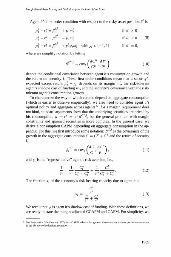
Figure 1 shows three interest rates: the interest rate obtaining in the ab-sence of constraints, and the collateralized and uncollateralized rates obtainingwith constraints. As is seen in the figure, the collateralized interest rate (solidline) can be substantially lower than the complete-market rate in the bad states,while the uncollateralized rate can be extremely high, indicating the high valueof capital to agentb. The difference between these rates is the shadow cost ofcapital, which can get close to 10%, as in the data that we present in the nextsection.

Figure2 plots the return spreads between the underlying security and twoderivatives. The derivatives are distinguished by their different margin require-ments: One has an intermediate margin requirementmmedium= 30%—lower

1997


Figure 1Collateralized and uncollateralized interest ratesThis figure shows how interest rates depend on the state of the economy as measured bycb, the fraction ofconsumption accruing to the risk-tolerant investor. Low values ofcb correspond to bad states of the economy, andmargin requirements bind forcb ≤ 0.22. The solid line represents the collateralized interest rater c (or Treasuryrate), which drops sharply in bad times. The dashed line represents the uncollateralized inter-bank interest rater u. As a frictionless benchmark, the dash-dot line represents the interest rate obtaining in an economy withoutany constraints.

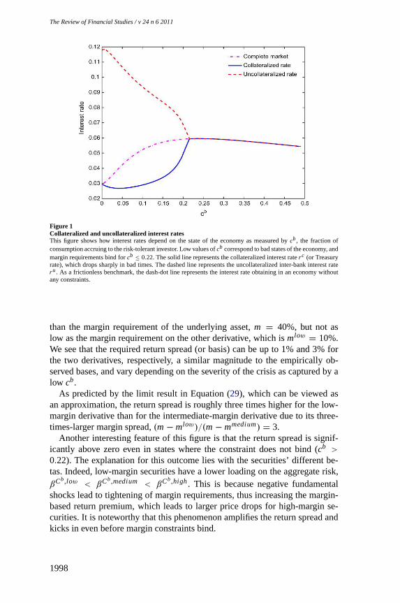
than the margin requirement of the underlying asset,m = 40%, but not aslow as the margin requirement on the other derivative, which ismlow = 10%.We see that the required return spread (or basis) can be up to 1% and 3% forthe two derivatives, respectively, a similar magnitude to the empirically ob-served bases, and vary depending on the severity of the crisis as captured by alow cb.

As predicted by the limit result in Equation (29), which can be viewed asan approximation, the return spread is roughly three times higher for the low-margin derivative than for the intermediate-margin derivative due to its three-times-larger margin spread,(m − mlow)/(m − mmedium) = 3.

Another interesting feature of this figure is that the return spread is signif-icantly above zero even in states where the constraint does not bind (cb >0.22). The explanation for this outcome lies with the securities’ different be-tas. Indeed, low-margin securities have a lower loading on the aggregate risk,βCb,low < βCb,medium < βCb,high. This is because negative fundamentalshocks lead to tightening of margin requirements, thus increasing the margin-based return premium, which leads to larger price drops for high-margin se-curities. It is noteworthy that this phenomenon amplifies the return spread andkicks in even before margin constraints bind.

1998


Figure 2Deviations from the law of one price (Basis)This figure shows the difference between the expected return of an underlying security and a derivative with thesame cash flows and a lower margin. This return spread is depicted as a function of the state of the economyas measured bycb (where a lowcb is a bad state of the economy). The dotted line represents the return spreadfor a low-margin derivativemlow with a high margin spreadmunderlying− mlow = 30%, and the dashed linerepresents a medium-margin derivative with a smaller margin spread ofmunderlying− mmedium= 10%.

Similarly, lower-margin securities have lower volatilities9 because they areless exposed to changes in the shadow cost of capital, i.e., they have less liq-uidity risk. The ratio of the risk (beta or volatility) of low-margin securitiesto high-margin securities is U-shaped. When constraints are far from binding(largecb), margins have little effect on returns, and the risks of high- and low-margin securities are similar. For lower values ofcb where constraints becomebinding, the risk difference becomes significant, but it eventually goes downasb-agents are wiped out (cb close to zero).

In addition, the dependence of the sensitivity to aggregate risk on the mar-gin size also implies that, once the idiosyncratic componentssi are taken intoaccount, the returns on low-margin securities are less highly correlated thanthose on high-margin securities, all else equal. Furthermore, the bases betweenunderlying-derivative pairs, driven largely by the common shadow cost of cap-ital, are more correlated with each other than the underlying securities are.

Figure 3 plots the Sharpe ratios (SR) of the underlying in an alternativeeconomy with no margin constraints, the underlying when there exist margin

9 In various calibrations, we found that higher-margin securities have larger betas and volatilities. We can showthis result in general using Malliavin-calculus techniques, provided that the ratioψ/cb decreases withcb. Whilethis ratio clearly decreases at bothcb = 0 andcb = sup{c

∣∣ ψ(c) > 0}, i.e., where the constraint just binds, we

could not prove that it does everywhere.

1999


Figure 3Sharpe ratios (SR)The figure shows how the required SR depends on the state of the economy as measured bycb (where a lowcb

is a bad state of the economy). The solid line represents the SR of the underlying asset with a high margin, thedashed line represents the SR of a derivative with identical cash flows and a medium margin, and the dotted linethat of a derivative with a low margin. As a frictionless benchmark, the dash-dot line represents the SR obtainingin an economy without any constraints.

constraints, and of the two derivatives. We see that the SR of the underlying ishigher with the constraint than without it to compensate for the cost of marginuse. The SR of the derivatives is lower than that of the underlying due to theirlower margins.

Finally, Figure4 shows the price premium of derivatives above the price ofthe underlying,Pderivative/Phigh − 1. We consider this quantity both for thelow- and medium-margin derivatives as well as for a varying-margin deriva-tive. The margin of the latter is 10% in “good states,” wherecb ≥ 0.15, andincreases to 30% in “bad states,” wherecb < 0.15. The price premia can bevery large, especially for low-margin securities in bad states of the economy.Interestingly, the price premia are significant even when the margin constraintsare not binding or even close to being binding. This is because the price reflectsthe possibility of future binding margin constraints, and puts a premium on se-curities with low margins in such states of nature. Since the random-marginsecurity has a high margin in the worst states, it is priced similarly to the high-margin security even when its margin is low.

Another way of looking at the price level is to consider how the price-dividend ratio depends on the state of the economycb. Our calibration yieldsthe natural outcome, also discussed above in footnote8, that the price-dividendratioζ is increasing incb, i.e., higher valuation ratios obtain in good times. (We

2000


Figure 4Price premiumThe figure shows how the price premium above the price of the underlying depends on the state of the econ-omy as measured bycb (where a lowcb is a bad state of the economy). Each derivative has the same cashflows as the underlying, but a lower margin requirement and, therefore, a larger price. The price premium,Pderivative/Punderlying − 1, is illustrated for a derivative with a low constant margin of 10%, one with amargin of 30%, and one that has a margin that increases from 10% to 30% in a bad state of the economy withcb < 0.15. The price premium is especially large for low-margin securities during bad economic times, but isnon-trivial even before margin requirements bind (cb > 0.22) due to the risk of future binding constraints.

omit the graph for brevity.) Conversely, the dividend yield (the reciprocal of theprice-dividend ratio) is lower in good times. In the empirical Section3.1below,we show that the dividend yield in the stock market is linked to the CDS–bondbasis, consistent with both depending on how constrained the economy is.

3. Empirical Applications

This section applies our model to the CDS–bond basis, the failure of thecovered interest-rate parity, the pricing of the Fed’s lending facilities, and toquantify the cost of capital requirements.

3.1 The CDS–bond basisThe CDS–bond basis is a measure of the price discrepancy between securitieswith nearly identical economic exposures, namely corporate bonds and CDS.Said simply, the CDS–bond basis is what one can earn by buying a corporatebond and a CDS that protects against default on the bond.10 Since this packagein principle has no risk if one can hold to maturity (though there are certain

10 Sometimes the CDS–bond basis is reported with the opposite sign. For simplicity, we use a convention thatimplies a positive basis during the crisis that started in 2007.

2001


risks in the real world), the basis reflects a deviation from the LoOP. However,to earn an arbitrage profit, one must use capital, and during a funding crisiscapital is required to earn excess returns for constrained investors, so this isconsistent with our margin-based asset pricing.

Another way of stating the apparent puzzle is to note that the yield spreadon a corporate bond is higher than the CDS spread. According to our model,this is because agents can get credit exposure with less use of margin capitalthrough CDS and, therefore, they are willing to earn a smaller expected returnper notional, but a similar return per use of margin capital.

To understand the difference in margin requirements of corporate bonds andCDSs, consider a hedge fund that buys a corporate bond. It must naturally usecapital to pay the bond’s price. The hedge fund can borrow using the bondas collateral, but this uses the hedge fund’s broker’s balance sheet. In light ofour model, all capital use by risk-tolerant agents is costly, so the question iswhether the broker can in turn borrow against the bond from an unconstrainedagent such a cash-rich commercial bank. This can be done only to a limitedextent if the commercial bank does not have experience trading such bonds,since corporate bonds are illiquid, making the evaluation of their value andrisk potentially difficult. Importantly, the bond’s market illiquidity also meansthat it can be difficult, time consuming, and costly to sell the bond during timesof stress.

A CDS, on the other hand, is a derivative with zero present value so it doesnot inherently use capital. A hedge fund entering into a CDS must neverthelesspost margin to limit the counterparty risk of the contract. Since the CDS marginreflects mostly the economic counterparty risk, whereas the corporate-bondmargin additionally reflects its inherent cash usage and market illiquidity, thecorporate-bond margin is larger than the CDS margin. In short, margins on“funded” underlying assets such as corporate bonds are larger than those of“unfunded” derivatives.

We test the model’s predictions for (i) the time series of the deviation fromthe LoOP; (ii) the cross-section of the LoOP deviations for different pairs ofCDS/bond; and (iii) the time series and cross-section of the risk (measured asvolatility and beta) of the CDSs and bonds. We first describe the data.

DataWe use data on the returns of the CDX index and S&P500 from Bloomberg,the Merrill Lynch intermediate corporate return indices in excess of the same-maturity swaps from Merrill Lynch, the average investment grade (IG) andhigh-yield (HY) CDS-bond bases from a major broker-dealer, LIBOR and GCrepo rates from Bloomberg, and the average dividend yield of U.S. stocks fromMSCI. Further, we use the Federal Reserve Board’s survey, “Senior Loan Of-ficer Opinion Survey on Bank Lending Practices,” focusing on the net percentof respondents tightening their credit standards.

2002


Figure 5The CDS–bond basis, the LIBOR-GC repo spread, and credit standardsThis figure shows the CDS–bond basis, computed as the yield spread for corporate bonds minus the CDS spread(adjusted to account for certain differences between CDS and bonds), averaged across high-grade bonds, as wellas the spread between the 3-month uncollateralized LIBOR loans and 3-month general collateral (GC) repo rate,and the net percent of respondents tightening their credit standards in the Federal Reserve Board’s “Senior LoanOfficer Opinion Survey on Bank Lending Practices.” Consistent with our model’s predictions, tighter credit isassociated with higher interest-rate spreads and a widening of the basis.

Testing the model’s time-series loOP predictionsTo consider our model’s time-series predictions, Figure5 shows the averageCDS–bond basis for high-grade bonds, the spread between the three-monthuncollateralized LIBOR loans and three-month GC repo rate, and the Fed’ssurvey measure of tightening credit standards.

We see that tighter credit standards (possibly reflecting more binding marginconstraints) are associated with higher interest-rate spreads and a wideningof the basis, consistent with our model’s predictions. The link between theinterest-rate spread and the basis, in particular, is related to Propositions4 and9, which describe the dependence of the basis on the shadow cost of capital,and Proposition1, linking the cost of capital to the interest-rate spread.

We test these predictions more formally in Table2. In particular, Panel Areports time-series regressions of the CDS–bond basis on, respectively, the T-bill–Eurodollar (TED) spread, the credit standards, and the average dividendyield of U.S. stocks. The dividend yield is the dividend of stocks, divided bytheir price, and it can be viewed as a measure of required returns. Specifically,in our calibration in Section2.2, a high dividend is associated with a poorstate of the economy where constraints are binding and deviations of the LoOPoccur. We include the dividend yield to address an additional prediction ofthe model, namely that the funding frictions affect required returns broadly,including in the stock markets.

We run these univariate regressions for the average basis both among IGsecurities and among HY securities. We see that both the IG and HY bases

2003


Table 2Time–series relation between CDS–bond basis and measures on liquidity and risk premia

Panel A: Regressions inLevels. Dependent Variable: CDS-Bond Basis.Investment Grade High Yield

coefficient t-statistic R2 coefficient t-statistic R2

TED spread 0.54 4.62 26% 0.86 3.78 19%Credit standards 0.02 13.60 75% 0.03 11.11 67%Dividend yield 1.62 21.03 88% 2.95 17.34 83%

Panel B: Regressions inChanges.Dependent Variable: CDS-Bond Basis.Investment Grade High Yield

coefficient t-statistic R2 coefficient t-statistic R2

TED spread 0.42 4.35 42% 0.72 4.32 33%Credit standards 0.02 4.12 47% 0.03 3.17 35%Dividend yield 1.06 3.83 23% 2.37 5.99 39%

The table reports univariate regressions of the CDS–bond basis on, respectively, the TED-spread (proxyingfor funding illiquidity) and the dividend yield of U.S. stocks as reported by MSCI (proxying for risk premia),monthly from 2005 to 2009, and the tightening credit standards from Federal Reserve Board’s survey, whichis available quarterly. We run these regressions separately for the average basis among investment-grade andhigh-yield bonds, and separately for the levels of these variables (Panel A) and the monthly changes of thevariables (Panel B), except the credit standards, which is run quarterly. To account for the potential bias due tostale prices in the monthly regression of changes, we include a lagged value of the explanatory variable (Dimson1979),basist = α+ β1xt + β2xt−1 + εt . We report the bias-corrected estimate,β1 + β2. The coefficient of theintercept is not reported.

load significantly on the first two measures of funding illiquidity as well as onthe dividend yield, as predicted by the model. The credit standard has anR2

as high as 75% for IG and 67% for HY, and the dividend yield has the highestR2, in excess of 80% for both IG and HY. While consistent with the model, itis surprising that the deviations from the LoOP in the credit markets appear soclosely linked not only to the funding markets, but even to the stock market.

While these results formalize the connection between the bases and the fund-ing measures that is visually clear in Figure5, there can be severe biases inconnection with regressions of persistence variables such as these. Runningthe regression in changes has better small-sample properties, as changes aremore stationary and, effectively, the sample has more independent observa-tions. Panel B of Table2 reports the regressions in changes. To account for thepotential bias due to non-synchronous trading (i.e., stale prices) in the monthlyregression of changes,11 we include a lagged value of the explanatory variable(following Dimson 1979and many others),

basist = α + β1xt + β2xt−1 + εt .

We then report the biased-adjusted slope coefficientβ1 + β2 and itst-statistic,estimated using the asymptotic variance-covariance matrix of (β1, β2). We seethat the coefficients remain highly significant for all the explanatory variables

11 As is standard, we do not add a lagged variable in regressions in levels, since this introduces colinearity problems,and non-synchronous trading has little effect on the regression in levels.

2004


and for both the IG and HY bases. The changes of the explanatory variablescontinue to have a high degree of explanatory power, withR2 values rangingfrom 23% to 47%.

The model’s prediction regarding the relation between the magnitude of theinterest-rate spread and the magnitude of the basis is rejected in the data, ifLIBOR is the true uncollateralized interest rate. Proposition9 predicts thatthe basis is the shadow cost of capital multiplied by a number less than 1, andProposition1 that the shadow cost of capital is equal to the interest-rate spread.However, the basis is in fact higher than the interest-rate spread at the end of thesample. This happens, most likely, because the financial institutions’ shadowcost of capital is larger than the LIBOR spread, for a couple of reasons: TheFed keeps the LIBOR down (see next section), many arbitrageurs (e.g., hedgefunds) cannot borrow at LIBOR, and even those that can borrow at LIBORcannot use a LIBOR loan to increase their trading, as they must limit theirleverage.

Testing the model’s cross-sectional loOP predictionsWe next test the model’s cross-sectional predictions for the deviation from theLoOP. For this, we compare the basis of IG bonds with that of HY bonds,as seen in Figure6. To facilitate the comparison in light of our model, we

Figure 6Investment grade (IG) and high yield (HY) CDS–bond bases, adjusted for their marginsThis figure shows the CDS–bond basis, computed as the yield spread for corporate bonds minus the CDS spread(adjusted to account for certain differences between CDS and bonds), averaged across IG and HY bonds, respec-tively. Our model predicts that the basis should line up in the cross-section according to the margin differences.Since IG corporate bonds have a margin around 25% and IG CDS have margins around 5%, the IG margindifferential is 20%. Hence, the adjusted IG basis is basis/0.20. Similarly, we estimate that the HY margin dif-ferential is around 50% so the HY adjusted basis is basis/0.50. We adjust the level of each series by subtractingthe average during the first two years, 2005–2006, when credit was easy so margin effects played a small role.Consistent with the idea that the expected profit per margin use is constant in the cross-section, we see that theadjusted bases track each other.

2005


adjust the bases for their relative margin spreads. Since IG corporate bondshave a margin around 25% and IG CDSs have margins around 5%, the IGmargin differential is 20%. Hence, the adjusted IG basis is basis/0.20. Similarly,we estimate that the HY margin differential is around 50%, so the HY ad-justed basis is basis/0.50. These margin rates are based on a broker’s estimates,which are subject to a substantial amount of uncertainty, since margins areopaque and vary between brokers and clients and over time. Propositions4and9 predict that the bases adjusted for margins in this way should line upin the cross-section so that the expected profit per margin use is constant inthe cross-section. Figure6 shows that the adjusted bases track each other quiteclosely.

We test the statistical significance of this cross-sectional relation in Table3.Panel A shows the regression of the HY basis on the IG basis, both in levels andin changes. For the change regression, we adjust for nonsynchronous prices asdescribed above and have the IG basis on the right-hand side, as it is based onthe more liquid instruments. We see that the close connection between IG andHY bases is highly statistically significant.

To further test the model’s cross-sectional predictions, Panel B reports thefollowing. First, we estimate the slope of the cross-sectional required return-margin curve at each point in time. Specifically, each month, we regress thetwo bases on the IG and HY margin differences (0.2, 0.5):

basisi = slope× (mi,bond − mi,C DS)+ εi . (32)

Table 3Cross-sectional relation between IG and HY bases

Panel A: Regressing the high-yield basis on the investment-grade basis.coefficient t-statistic R2

LevelsIG basis, levels 1.79 25.53 91%

ChangesIG basis, changes 1.42 8.27 64%

Panel B: Regressing the slope of the margin-return curve on explanatory variables.coefficient t-statistic R2

LevelsTED spread 1.86 3.95 20%Credit standards 0.07 11.71 69%Dividend yield 6.19 18.61 85%

ChangesTED spread 1.53 4.54 37%Credit standards 0.07 3.39 38%Dividend yield 4.81 5.78 38%

Panel A reports the regression of the high-yield (HY) CDS–bond basis on the investment-grade (IG) CDS–bondbasis. We note that the IG securities are more liquid and, to account for the potential effect of stale prices in theregression of changes, we include a lagged value of the explanatory variable (Dimson 1979),basisHY

t = α +

β1basisI Gt + β2basisI G

t−1 + εt . We report the bias-corrected estimate,β1 + β2. In Panel B, we first estimate theslope of the cross-sectional required return-margin relation at any time. We do this by regressing the two baseson the two corresponding margin differences (0.20, 0.50). We then regress this slope (which measures fundingilliquidity according to the model) on the three explanatory variables described in Table 2.

2006


Table 4Volatility of CDS vs. bonds

Investment Grade High Yield

CDS Bonds CDS Bonds

Early sample 0.57% 0.51% 3.73% 2.76%Crisis 3.92% 10.26% 17.19% 20.87%

Full sample 3.02% 7.83% 13.31% 16.01%

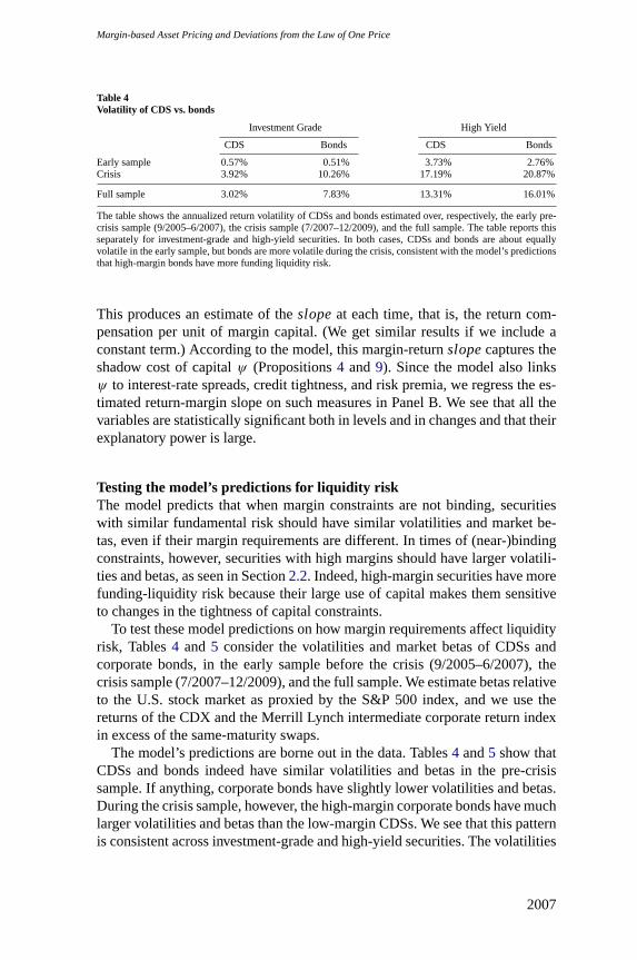
The table shows the annualized return volatility of CDSs and bonds estimated over, respectively, the early pre-crisis sample (9/2005–6/2007), the crisis sample (7/2007–12/2009), and the full sample. The table reports thisseparately for investment-grade and high-yield securities. In both cases, CDSs and bonds are about equallyvolatile in the early sample, but bonds are more volatile during the crisis, consistent with the model’s predictionsthat high-margin bonds have more funding liquidity risk.

This produces an estimate of theslopeat each time, that is, the return com-pensation per unit of margin capital. (We get similar results if we include aconstant term.) According to the model, this margin-returnslopecaptures theshadow cost of capitalψ (Propositions4 and9). Since the model also linksψ to interest-rate spreads, credit tightness, and risk premia, we regress the es-timated return-margin slope on such measures in Panel B. We see that all thevariables are statistically significant both in levels and in changes and that theirexplanatory power is large.

Testing the model’s predictions for liquidity riskThe model predicts that when margin constraints are not binding, securitieswith similar fundamental risk should have similar volatilities and market be-tas, even if their margin requirements are different. In times of (near-)bindingconstraints, however, securities with high margins should have larger volatili-ties and betas, as seen in Section2.2. Indeed, high-margin securities have morefunding-liquidity risk because their large use of capital makes them sensitiveto changes in the tightness of capital constraints.

To test these model predictions on how margin requirements affect liquidityrisk, Tables4 and5 consider the volatilities and market betas of CDSs andcorporate bonds, in the early sample before the crisis (9/2005–6/2007), thecrisis sample (7/2007–12/2009), and the full sample. We estimate betas relativeto the U.S. stock market as proxied by the S&P 500 index, and we use thereturns of the CDX and the Merrill Lynch intermediate corporate return indexin excess of the same-maturity swaps.

The model’s predictions are borne out in the data. Tables4 and5 show thatCDSs and bonds indeed have similar volatilities and betas in the pre-crisissample. If anything, corporate bonds have slightly lower volatilities and betas.During the crisis sample, however, the high-margin corporate bonds have muchlarger volatilities and betas than the low-margin CDSs. We see that this patternis consistent across investment-grade and high-yield securities. The volatilities

2007


Table 5Betas of CDS vs. bonds

Panel A: Betas estimated separately for CDS on BondsInvestment Grade High Yield

CDS Bonds CDS Bonds

Early sample 0.05 −0.01 0.35 0.22(stand, err.) (0.01) (0.02) (0.09) (0.08)

Crisis 0.13 0.29 0.56 0.73(stand, err.) (0.02) (0.07) (0.10) (0.12)

Full sample 0.12 0.26 0.54 0.69(stand, err.) (0.02) (0.05) (0.08) (0.09)

Panel B: Panel regression with CDS and bondsr it = α + α ∙ 1[i =bond] + βr M K T

t + βr M K Tt ∙ 1[i =bond] + εi

t

Investment Grade High Yield

MKT 0.12 0.54(t-statistic) (3.17) (6.48)

MKT* 1 (Bond) 0.14 0.15(t-statistic) (2.60) (1.28)

Panel A shows the market betas of CDS and bond returns estimated over, respectively, the early pre-crisis sample(9/2005–6/2007), the crisis sample (7/2007–12/2009), and the full sample. The table reports this separately forinvestment-grade and high-yield securities. In both cases, bonds have slightly lower betas in the early sample,but bonds have larger betas during the crisis, consistent with the model’s predictions that high-margin bondshave more funding liquidity risk. Panel B shows the statistical significance of the difference between CDSs andbonds using a panel regression.

are estimated with precision (the standard errors of these numbers are a fewpercentage points), and the difference between bonds and CDSs is significant(not reported for brevity). The difference between the bond and CDS betas istested in Panel B of Table5, and we see that the difference is significant for IGsecurities.

3.2 Effects of monetary policy and lending facilitiesThe Federal Reserve has tried to alleviate the financial sector’s funding cri-sis by instituting various lending facilities. These programs include the TermAuction Facility (TAF), the Term Securities Lending Facility (TSLF), the TermAsset-Backed Securities Loan Facility (TALF), and several other programs.12

The TAF was instituted in December 2007 in response to the “pressures inshort-term funding markets.” With the TAF, the Fed auctions collateralizedloans to depository institutions at favorable margin requirements with 28-dayor 84-day maturity.

As the crisis escalated, the Fed announced on March 11, 2008, the TSLF,which offers Treasury collateral to primary dealers in exchange for otherprogram-eligible collateral, such as mortgage bonds and other IG securities for28 days. Since this is an exchange of low-margin securities for higher-marginsecurities, it also improves the participating financial institutions’

12 We thank Adam Ashcraft, Tobias Adrian, and participants in the Liquidity Working Group at the New York Fedfor helpful discussions on these programs.

2008


funding condition. By exchanging a mortgage bond for a Treasury and thenborrowing against the Treasury, the dealer effectively has its margin on mort-gage bonds reduced.

The Federal Reserve announced the additional creation of the TALF onNovember 25, 2008. The TALF issues nonrecourse loans with terms up tothree years of eligible asset-backed securities (ABS) backed by such thingsas student loans, auto loans, credit card loans, and loans relating to businessequipment. The TALF is offered to a wide set of borrowers, not just banks (butthe borrowers must sign up with a primary dealer, which creates an additionallayer of frictions).

These programs share the feature that the Fed offers lower margins than areotherwise available in order to improve the funding of owners or buyers ofvarious securities. This improves the funding condition of the financial sectorand, importantly, makes the affected securities more attractive than they wouldbe otherwise. Indeed, the goal of the TALF is to “help market participants meetthe credit needs of households and small businesses by supporting the issuanceof asset-backed securities.”13

In terms of our model, this can be understood as follows. The Fed offers amarginmi,Fed for securityi , say, a student-loan ABS, which is lower than theprevailing margin,mFed,i < mi . This lowers the required return of a derivativesecurity:

E(r i,Fed)− E(r i,no Fed)= (mFed,i − mi )ψ Fed + (ψ Fed − ψnoFed)mi

+ (β i,Fed − β i,noFed) < 0. (33)

Said differently, the Fed program increases the affected security’s price (Propo-sition5). Hence, this ABS can be issued at an increased price, which makes themarket more viable, given the inability of, say, students, to pay a high interestrate.

Ashcraft, Garleanu, and Pedersen(2010) provide survey evidence fromfinancial institutions to see how their bid prices for various securities depend onthe financing that the Fed would offer. The surveyed bid price increases as theFed reduces its offered margin, consistent with our model. For instance, thesurveyed bid price of a super senior collateralized mortgage-backed security(CMBS) tranche with an expected life of seven years with no Fed financing is$57, but increases to $92.5 with maturity matched financing with a low margin,a very large asset-pricing effect. Similarly, the bid price of a tranche with 2.5years of expected life increases from $84 with no financing to $92 with financ-ing with a low margin. This corresponds roughly to an annualized decrease inexpected return of 3.5%.

Let us consider this number in the context of our model. If the shadow costof capital is around 10%, as implied by the IG and HY CDS–bond bases at the

13 See http://www.newyorkfed.org/markets/talf operations.html.

2009


height of the liquidity crisis, and CMBS tranches are derivatives only held bythe risk-tolerant investor, then the key first term in Equation (33) implies aneffect of 3.5% if the Fed improves the margin terms by 35 percentage points,so the model-implied effect is in the right neighborhood.

Ashcraft, Garleanu, and Pedersen(2010) also provide evidence that theTALF lending facility had an impact on the market prices of CMBS bondsin a way that is consistent with our model.

3.3 Failure of the covered interest-rate parity and the fed’s liquidityswap lines

While textbooks on international finance acknowledge the failure of the un-covered interest-rate parity, the covered interest-rate parity is often taken tohold by definition, since arbitrage should enforce the LoOP. The CIP says thatif the local interest rate isr , the foreign interest rate isr ∗, the spot exchangerate ise, and the forward exchange rate that can be locked in now isf , then1+ r = f/e(1+ r ∗). That is, putting the money in the local bank earns 1+ r ,which should be the same as exchanging a dollar for 1/e units of foreign cur-rency, earning 1+ r ∗ abroad, and guaranteeing to exchange the money back atthe rate off to get f/e(1 + r ∗).

This parity has nevertheless failed due to supply and demand imbalances inthe forward market and because it requires capital (margin) to trade to profitfrom deviations from parity. To understand the background of this surprisingeffect, recall first that the funding problems of financial institutions in the crisisof 2007–2009 quickly spread globally. Banks in many countries had fundingproblems both in their local currency and in U.S. dollars, perhaps becausemany transactions are done in dollars.

To facilitate dollar funding for foreign banks, the Fed authorized temporaryreciprocal currency arrangements called “central bank liquidity swap lines” onDecember 12, 2007 (Coffey, Hrung, Nguyen, and Sarkar 2009). Through theseswap lines, the Fed lent dollars to foreign central banks, which in turn lentthese dollars to their local banks.

Despite this effort, parity has been violated as a clear sign that the currencyarbitrageurs’ margin requirements are binding, as seen in Figure7. The fig-ure further shows that the time-series pattern of the deviation tracks the TEDspread in the 2007–2009 crisis and in the liquidity crisis of 1998 (involvingLong-Term Capital Management, among other events). This co-movement ishighly statistically significant both in levels and in monthly changes (regres-sions are not shown for brevity).

3.4 Quantifying the cost of capital requirements: Incentives forregulatory arbitrage

We can also use our model to quantify the shadow cost of Basel capital require-ments in order to help understand the banks’ incentives to perform “regulatory

2010


Figure 7Average deviation from covered interest-rate parity and the TED spreadThis figure shows the average absolute deviation from the covered interest-rate parity for the Euro, Yen, andBritish Pound, as well as the TED spread, which is the 3-month uncollateralized LIBOR rate minus the 3-monthT-bill rate. The magnitude of the deviation from the CIP tracks the TED spread in the time series consistent withthe model’s prediction that the shadow cost of funding liquidity due to binding margins drives both effects.

arbitrage” by moving assets off their balance sheets and tilting their portfoliostoward AAA securities with low regulatory capital requirements.

For this, we note that the Basel requirement has a similar form to the marginrequirement. It can loosely be captured by a similar equation to our model’smargin requirement (seeBrunnermeier and Pedersen 2009):

∑

i

mReg,i |θ i | ≤ 1, (34)

whereθ i is the fraction of wealth in securityi as before andmReg,i is theregulatory capital requirement (8% times a risk weight under some rules).

When the prevailing margins are low, the regulatory requirement may bemore binding than the funding-based margin requirement. In this case, themarginmi in our pricing formula is replaced by the regulatory requirementin Equation (34). Hence, a bank’s required return increases in the regulatorycapital requirement multiplied by the shadow cost of capital,ψmReg,i . If theshadow cost of regulatory capital is 1% and a bank can move off balance sheetan asset with risk weight of 100%, then its required return for that asset isreduced by 1%× 8%× 100%= 80 basis points.

4. Conclusion

We derive a tractable general-equilibrium asset-pricing model that accountsexplicitly for the pricing of margins. The model captures several of the salient

2011


features of the recent and past liquidity crises: A negative fundamental shockleads to losses for leveraged agents, including the financial sector; these agentsface funding problems as they hit margin constraints; and the binding con-straints lead to drops in Treasury rates and GC interest rates, to spikes ininterest-rate spreads, risk premia, and the pricing of margins, and to bases (orprice gaps) between securities with identical cash flows but different margins.

We illustrate the model through a calibration, test it empirically using theCDS–bond basis and the failure of the covered interest-rate parity, and showhow the model-implied cost of capital requirements quantifies the banks’ in-centives to use off-balance-sheet vehicles. Finally, we estimate the effect ofthe Fed’s lending facilities, which is helpful in evaluating the unconventionalmonetary policy tools used during liquidity crises.

Appendix

A Linear and nonlinear margin constraintsWe consider a nonlinear margin requirement, given in Equation (7), that depends on the absolutevalue of the position|θ i |. Hence, both long (θ i > 0) and short (θ i < 0) positions make theconstraint tighter, i.e., both long and short positions use capital. It is interesting to compare thiswith a linear constraint sometimes assumed in the literature:

∑

i

mit θ

i + ηu ≤ 1. (A.1)

While such a linear constraint is simpler to handle mathematically, it precludes the bases that arecentral to our study:

Proposition 10. If agents face only linear margin requirements (A.1) and at least one deriva-

tive exists withmi ′ < mi , then any equilibrium is as if there were no margin constraints at all andthere can be no deviations from the Law of One Price in equilibrium; that is, the basis is alwayszero.

Proof of Proposition 10. For any asset allocations of the two agents, the linear margin constraintis slack “in the aggregate”:

Wat

∑

j

mjt θ

j,at + Wb

t

∑

j

mjt θ

j,bt < Wa

t + Wbt . (A.2)

This means that the linear margin constraint must be slack for at least one of the agents, who istherefore not constrained at timet .

Suppose now that on a non-zero-measure set there fails to exist a market-price-of-risk process,

i.e., a processκ taking values inRN such thatσ jt κt = μ

jt − r c

t for all securitiesj . Then one ofthe two agents can trade on a non-zero-measure set to make riskless strictly positive (althoughbounded) profits—i.e., a zero-value portfolioη exists whose volatility is zero and that has strictlypositive drift. This contradicts the notion of equilibrium. Consequently, a market-price-of-riskprocess exists. It follows, under technical integrability conditions, that an equivalent martingalemeasure, defined by the stochastic exponential of this process, also exists, so that assets withidentical cash flows have identical payoffs. (SeeDuffie 2001, Chapter 6, Section G.)

2012


Finally, consider two securities,i and j , with identical cash flows and prices but different

margin constraints:mit > mj

t on some set. If any agent is constrained whenmit > mj

t , thenshe can relax her constraint by going longn shares of assetj and shortn shares of asseti : Thetrade has no cash-flow implications and makes the constraint slack. Forn low enough, the otheragent’s margin constraints remain slack due to (A.2), and therefore both agents are unconstrained,while their consumption processes remain the same. (Alternatively, we can note that the CAPMrelationshipμi

t − r ct = βg, j + ψ

gt mi

t impliesψgt = 0 for both agentsg ∈ {a, b}.) �

B ProofsProof of Propositions1 and 4. These proofs are in the body of the article. �

Rather than offering a proof to the special Proposition2, we state and prove its general ver-sion. To this end, we define the risk-tolerance fraction due to agenta by xt = 1−xt . We recall thatψ is agentb’s shadow cost of funding, and we denotea’s shadow cost of funding byψ . Finally,yi indicates whetherb is long (yi

t = 1), is short (yit = −1), or has no position (yi

t ∈ [−1, 1]) inan asset, and similarlyyi indicates the sign ofa’s position.Proposition 2′ (Margin CCAPM). The expected excess returnμi

t − r ct on an underlying asset

is given by the standard consumption CAPM adjusted for funding costs:

μit − r c

t = γtβC,it + λm,i

t mit , (B.1)

where the funding cost is the product of the margin requirement and the margin premium:

λm,it = xt ψt yi

t + xtψt yit . (B.2)

�Proof of Proposition 2′. To understand the idea of the proof, suppose first that agenta’s marginconstraint never binds, so that he is (locally) unconstrained in his investment in the underlyingassets. Consequently, deflating the gains process of any of these securities using his marginalutility process yields a local martingale. Specifically, agenta’s marginal utility, which we denoteby ξt , is given by

ξt = e−ρt (Ca)−γa. (B.3)

Further, we denote its drift and volatility byμξt andσξt :

dξt = ξt

(μξt dt + σ

ξt dwt

), (B.4)

and Ito’s Lemma shows thatσξ = −γ aσCa

. (B.5)

The discounted value of the price and accumulated dividends,

Pt ξt +∫ t

0Csξs ds, (B.6)

is a local martingale, so it has zero drift:

0 = δit + Pit μ

ξt + Pi

t μit − δit + Pi

t σit

(σξt

)>. (B.7)

Sinceξ prices the risk-free collateralized lending, it holds that

μξt = −r c

t . (B.8)

Combining Equations (B.5), (B.7), and (B.8) gives agenta’s key pricing equation:

μi − r c = γ aβCa,i . (B.9)

2013


Recall also agentb’s pricing equation:

μi − r c = βCb,i + yiψmi . (B.10)

Multiplying Equations (B.9) and (B.10) by (γ a)−1Ca andCb, respectively, and adding the resultsgives

(μi − r c)

(Ca

γ a + Cb)

= CβC,i + Cbyiψmi ,

which is equivalent to (14).The general proof of this proposition involves characterizing the optimal portfolio choice of

an arbitrary agent with utility functionu who faces convex portfolio constraints and redundantassets. The steps are the following:

Step 1.Construct a family of fictitious economies in which there are no redundant securities(derivatives) and where the drifts of asset prices and the (collateralized) interest rate are given, forν ∈ RN , by

μi,ν = μi + νi + h(ν)

r c,ν = r c + h(ν),

which are to be explained shortly. For ease of exposition, define alsoκν = σ−1(μ+ ν− r c) to bethe market price of risk for the underlying securities in the fictitious market and let

νi ′,ν = σ i ′κν + r c − μi ′

for all derivativesi ′. Definingμi ′,ν analogously toμi,ν would mean that there would be no arbi-trage opportunity in the fictitious market even if the redundant securities were traded.

For anyν ∈ RN , the functionh is defined as

h(ν) = sup

−

∑

i

θ i νi +∑

i ′θ i ′νi ′,ν

∣∣ θ ∈ K

= sup

−

∑

i

θ i νi +∑

i ′θ i ′σ i ′σ−1ν

+

∑

i ′θ i ′((μi ′ − r c)− σ i ′κ0

) ∣∣ θ ∈ K

.

The functionh(ν) captures both the shadow value of capital and the increase in the interest ratethat an agent would have to be offered in a world without redundant securities in order to achievethe same utility as when arbitrage opportunities are available to him. The first term in the lastexpression above represents the total additional return due to the higher drifts in the fictitiouseconomy, while the second represents the arbitrage gains. Note that, sinceK is bounded,h takesfinite values onRN .

The fictitious economies are constructed so that any consumption feasible in the original,constrained economy starting with a certain wealth is also feasible in each of these economies—because available returns are at least as high. By including all such economies, it also followsthat there is one among them in which the optimal portfolio and consumption choices satisfy theoriginal constraints.

Step 2.For any consumption plan, the trading strategy{φi }i that attains it at the highest cost(initial wealth) among the optimal strategies in all fictitious economies is equivalent, in terms

2014


of risk exposure, to a strategy({θ i }i , {θ i ′ }i

′)

that finances the consumption plan at the same

cost and satisfies the constraints in the original economy. This is the new step relative to theliterature.

To prove this statement, followCvitanic and Karatzas(1993) to define the maximum cost of(super-)replicating the consumption plan among all fictitious economies, from any timeτ onward:

Vτ ≡ supν

Eν[∫ T

τe−

∫ Tt r c,ν

s dsct dt

]

,

whereEν is the equivalent martingale measure in the market defined byν, given by the state-pricedeflatorξν , which is defined byξν(0) = 1 and

dξνt = −ξνt(r c,νdt +

(κν)> d Bt

).

It follows that

Mνt ≡ Vt e

∫ t0 r c,ν

s ds

is a supermartingale, so that it can be decomposed as

Mνt = V0 +

∫ t

0φνs dwνs − Bνt , (B.11)

with Bνt an increasing process andwν a Brownian motion. ComparingMν with M0 identifiesφν

as being independent ofν—let’s denote it byφ—and it also implies

∫ t

0e∫ s0 r c,νv dvd Bνs −

∫ t

0e∫ s0 r c,νv dvVs

(h(νs)+ ν>

s φ)

ds=∫ t

0e∫ s0 r cv dvd B0

s . (B.12)

We claim that, since the right-hand side of (B.12) is increasing,φ is equivalent to a strategyθ ∈ K . Indeed, suppose that this is not the case. The strategies in the original market that are riskequivalent toφ areθ = (θ , θ ), such that

φ = θ +(σ−1

)>σ>θ ,

where σ is the matrix of volatility vectors of the redundant securities. If the affine spaceΘφ

consisting of all suchθ does not intersect the compact convex setK , then it is separated from itby a hyperplane, i.e., there exist a vectorv andε > 0 such that

v>θ − v>θK ≥ ε

for all θ ∈ Θφ andθK ∈ K . Note thatv is orthogonal toΘφ , i.e., v>(θ1 − θ2) = 0 for allθ1, θ2 ∈ Θφ . In fact, v>θ = v>(φ, 0) onΘφ , andv> is a linear combination of the rows of

(IN ,(σ−1

)>σ>):

v> = v>(IN ,(σ−1

)>σ>)

for somev ∈ RN .Note now that

h(ν) = sup

−ν>

(θ +

(σ−1

)>σ>θ

)+∑

i ′θ i ′((σ i ′)>

κ0 − (μi ′ − r c)

) ∣∣(θ , θ

)∈ K

.

2015


Let ν = Rv for some (large) scalarR, and note also that

h(ν)+ ν>φ ≥ sup

{−ν>

(θ +

(σ−1

)>σ>θ

) ∣∣(θ , θ

)∈ K

}+ ν>φ +

sup

∑

i ′θ i ′((μi ′ − r c)− σ i ′κ0

) ∣∣(θ , θ

)∈ K

≥ sup

{−Rv>

(I ,(σ−1

)>σ>

)θ∣∣ θ ∈ K

}+ Rv>(φ, 0)+ D

≥ Rε + D,

where|D| < ∞ becauseK is bounded.Thus, ifΘφ ∩ K = ∅, thenh(ν) + ν>φ can be made arbitrarily large, and consequently

the left-, and therefore right-hand, side of (B.12) can be made decreasing, which would be acontradiction.

Step 3.The optimal consumption in the original economy is therefore optimal in one of thefictitious, unconstrained economies. Consequently, the marginal utility of the agent is proportionalto ξν , giving

u′′(Cg)

u′(Cg)CgσCg

= σ−1(μ− r c + ν),

or

μi − r c = γβCg,i − νi . (B.13)

Step 4.Forν that defines the constrained optimum, the optimalθ attains the supremum in thedefinition ofh(ν). The characterization ofν then comes down to a simple linear optimization overa convex set.

Suppose, for instance, thatθ1 > 0, which impliesν1 ≤ 0, and letψ = − ν1

m1 .14 If θ2 > 0

and, say,ν2

m2 > −ψ , decreasingθ2 by m1ε and increasingθ1 by m2ε preserves the constraints

but increases the objective by(ν2

m2 + ψ)

m1ε > 0. Thus, νi

mi = −ψ wheneverθ i > 0, so that

(B.13) becomes

μi − r c = γβCg,i + ψmi . (B.14)

All other cases are treated similarly. Note also thath(ν) = ψ .

As for the derivatives, from the definition ofνi ′ we have the relationship

μi ′ − r c = σ i ′σ−1(μ+ ν − r c)− νi ′

= γβCg,i ′ − νi ′ .

Therefore, the treatment of the derivative is the same as that of any underlying asset as longas the derivative position is not bound by a different constraint, which is entirely natural. If the

derivative positions are constrained by other constraints, then the form of the “shadow returns”νi ′

is different. �The next result is the general form of Proposition3.

Proposition 3′ [Margin CAPM]. The expected excess returnμit − r c

t on an underlying asset is

given by the standard CAPM adjusted for funding costs based on the margins mit :

μit − r c

t = λβt β

it + λm,i

t mit , (B.15)

14 RememberK = {θ |∑

i |θ i |mi ≤ 1}.

2016


whereλβt = μqt − r c

t −∑

j q jt λ

m, jt mj

t is a covariance risk premium and the margin premium

λm,i is defined in Proposition2′. �Proof of Proposition 3′. The definition of the portfolioq implies that

dCt

Ct= Qt

d Pqt

Pqt

+ dzt

for some processQ and Brownian motionz with covt (d Pi , dz) = 0 for all i . Proposition2therefore implies that

μit − r c

t − λm,it mi

t = Qt covt

(d Pq

t

Pqt,

d Pit

Pit

)

. (B.16)

Multiplying this equation byqit and summing over alli yields

μqt − r c

t −∑

i

qit λ

m,it mi

t = Qt vart

(d Pq

t

Pqt

)

. (B.17)

Equations (B.16) and (B.17) immediately give the proposition. �Proof of Proposition 5. Write the agent’s objective as

E∫ ∞

te−ρs

u(Cgs )− λs

∑

j

|Wsθj

s |mjs + Wsη

us − Ws

ds,

whereλ is a Lagrange multiplier. (In the case of agentb, the HJB equation showsλ to equal(ρW)−1ψ .) The agent acts as if unconstrained, provided thatλ is chosen appropriately.

Suppose that the agent invests inε more shares of asseti , borrowing at the collateralized rateto do so. The agent adjusts consumption to absorb both the dividends and the interest expense.Note that the only terms entering the constraint affected by this deviation are|Wsθ

is| and Ws.

Letting ε tend to zero, the gain in utility is proportional to

sign(ε)Et

∫ ∞

te−ρs

(u

′(Cg

s )(δis − r c

s Pit )− λs

(ysPi

smis − (Pi

s − Pit )))

ds

= sign(ε)Et

∫ ∞

te−ρs

(u

′(Cg

s )(δis − r c

s Pit )− λsPi

t + Pisλs

(1 − ysmi

s

))ds,

whereys = 1 if θ is > 0, ys = −1 if θ i

s < 0, andys = sign(ε) if θ i = 0. Since the deviation must(weakly) reduce utility regardless of the sign ofε, it follows that

Pit Et

∫ ∞

te−ρs

(u

′(Cg

s )rcs + λs

)ds = Et

∫ ∞

te−ρs

(u

′(Cg

s )δis + Pi

sλs

(1 − ysmi

s

))ds,

(B.18)whereys = 1 if θ i

s > 0, ys = −1 if θ is < 0, andys ∈ [−1, 1] if θ i

s = 0. Equation (B.18) implies

Pit Et

∫ ∞

te−ρ(s−t)

(u

′(Cg

s )rcs + λs

)ds = Et

∫ ∞

te−ρ(s−t)+

∫ st e−ρvλv(1−yvmi

v) dvu′(Cg

s )δis ds.

(B.19)Alternatively,u

′(Cg

s )rcs+λs in the previous two equations can be replaced withu

′(Cg

s )rus . Further,

under mild regularity conditions, the left-hand sides of these equations equalPit u

′(Cg

t ).The proposition follows from the fact that the right-hand side of Equation (B.19) is a mono-

tonic function ofyvmiv for all v ≥ t . �

2017


Proof of Proposition 6. We first derive the dynamics of the state variablecb and the consumptiondynamics more generally. Then we derive the dependence of the endogenous variables on the statevariables and the exogenous variables.

The dynamics of agentb’s consumptionCb follow from Cb = ρWb and the dynamics forWb given in (6):

dCb = Cb((r c − ρ + φκ) dt + φ dwt ), (B.20)

whereφ ≡ σθb is the notation for the equilibrium volatility of agentb’s wealth. Using this, thedynamics of the consumption ratiocb = Cb/C are seen to be

dcb = cb((r c − ρ + φκ − μC − σCφ + (σC)2) dt + (φ − σC) dwt ), (B.21)

while agenta’s consumption dynamicsCa = C − Cb are

dCa = (CμC − Cb(r c − ρ + φκ)) dt + (CσC − Cbφ) dwt (B.22)

= C(μC − cb(r c − ρ + φκ)) dt + C(σC − cbφ) dwt . (B.23)

The interest rate isr ct = −μξt (as seen in (B.8)), and thus applying Ito’s Lemma to the

marginal utilityξ from (B.3) implies

r c = ρ +

γ a μC − cbφκ

1 − cb−

1

2γ a(γ a + 1)

(σC − cbφ

1 − cb

)2

1 − cb

1 + (γ a − 1)cb.

The ordinary differential equation (ODE) that characterizes the price-dividend ratioζ(cb)

follows from the fact that (B.6) is a local martingale with zero drift:

0 = 1 + ζ(μC − rc − γ aσC(1 − cb)−1(σC − cbφ)

)+ (B.24)

ζ ′(rc − ρ + φκ − μC − γ a(φ − σC)(1 − cb)−1(σC − cbφ)

)+

1

2ζ ′′(cb)2(φ − σC)2.

It remains to determine the values ofκ, σ , andφ as functions ofζ and its derivatives. Forthis, we identify three equations for these three unknowns. First, the log-utility investor’s optimalpositionθb maximizes

(μ− r )θb −1

2σ2(θb)2,

subject toθb < m−1. Or, expressed in terms of volatilityφ = σθb, he maximizes

κφ −1

2φ2,

so that the optimal position is

φ = min(κ,m−1σ) = κ − (κ − m−1σ)+. (B.25)

Next, since agenta is unconstrained with respect to the market asset and general-collaterallending and borrowing, (B.9) gives

κ = γ aσCa

= γ a σC − cbφ

ca

= γ a σC − cbκ + cb(κ − m−1σ)+

1 − cb,

2018


where the second equality is due to the expression for the volatility ofCa in (B.23) and the thirdto (B.25). It follows that

κ =γ a

1 + (γ a − 1)cb

(σC + cb(κ − m−1σ)+

)

= κ + γ cb(κ −

σ

m

)+, (B.26)

with γ−1 = ca (γ a)−1 + cb as per (12) and κ = γ σC . Equation (B.26) provides a secondrestriction on the three parameters that need to be calculated. The third restriction comes from thefact that the volatilityσ of the pricePt = Ct ζ(cb

t ) is given by Ito’s Lemma and the dynamics ofcbt in (B.21):

σ = σC +ζ ′cb

ζ(φ − σC). (B.27)

To solve the system of three equations (B.25)–(B.27), φ can be eliminated right away to give

κ − m−1σ = (κ − m−1σ)+ γ cb(κ − m−1σ)+

σ = σC +ζ ′cb

ζ(κ − σC)−

ζ ′cb

ζ(κ − m−1σ)+,

and note that the solution(κ, σ ) given in the proposition is trivially true ifκ ≤ m−1σ , whichrequires thatκ ≤ m−1σ . Suppose therefore thatκ − m−1σ > 0, leaving a linear system ofequations. This system can be written as

κ − κ =1

1 − γ cb(κ − m−1σ)+ m−1σ − κ

=γ cb

1 − γ cb(κ − m−1σ)

σ − σ = −ζ ′cb

ζ(κ − m−1σ),

which gives (21) and (22) easily.The boundary values forζ(cb) are its values atcb = 0 andcb = 1. These are the price-

dividend ratios in the single-agent economies in which either agenta or agentb has all the wealth.The explicit expressions are well known:

ζ(0) =(ρ + (γ a − 1)μC −

1

2γ a(γ a − 1)

(σC)2)−1

(B.28)

ζ(1) = ρ−1. (B.29)

Finally, the value of the Lagrange multiplierψ follows from the first-order condition (9),

given the optimal choiceσCb= φ:

ψ =1

m(μ− r c − βCb

) =1

m(μ− r c − σCb

σ)

=σ

m(κ − σCb

) =σ

m(κ − φ)

=σ

m

(κ −

σ

m

)+. (B.30)

�

2019


Proof of Proposition 7. From Proposition4,

μi ′ = μ+ σC(σ i ′ − σ)+ ψ(mi ′ − m),

and applying Ito’s Lemma toPi ′ = Cζ i ′ (cb) gives

μi ′ =ζ i ′ ′cb

ζ i ′

(r c − ρ + φκ − μC

)+ μC +

1

2

ζ i ′ ′′(cb)2

ζ i ′(φ − σC)2 +

1

ζ i ′

σ i ′ =ζ i ′ ′cb

ζ i ′(φ − σC)+ σC .

Together, these three equations and (B.30) yield the ODE (26). The boundary conditions are

ζ i ′ (0) =(

yi ′)−1

ζ i ′ (1) = ρ−1,

where the dividend yieldyi ′ = y +μi ′ −μ = y +ψ(mi ′ − m) andy is the market dividend yieldatcb = 0, i.e.,y = ζ(0)−1 from Equation (B.28). �

Proof of Proposition 8. The limit price follows directly from Equation (B.28). The limit valueof ψ follows from (24), given thatσ = σC (because the market price isC times a constantprice-dividend ratio in the limit) andκ = γ aσC , which is seen from (21) with x = 0 andγ = γ a. �

Proof of Proposition 9. Only the risk inC is priced. In the limit ascb → 0, all valuation ratiosare constant, and therefore all covariances with the market equal(σC)2, so the result follows fromProposition4 with equal betas. �

ReferencesAcharya, V. V., and L. H. Pedersen. 2005. Asset Pricing with Liquidity Risk.Journal of Financial Economics77:375–410.

Acharya, V. V., and S. Viswanathan. 2011. Leverage, Moral Hazard, and Liquidity.Journal of Finance66:99–138.

Adrian, T., and H. Shin. 2010. Liquidity and Leverage.Journal of Financial Intermediation19:418–37.

Aiyagari, S., and M. Gertler. 1999. Overreaction of Asset Prices in General Equilibrium.Review of EconomicDynamics2:3–35.

Allen, F., and D. Gale. 1998. Optimal Financial Crisis.Journal of Finance53:1245–84.

Amihud, Y., and H. Mendelson. 1986. Asset Pricing and the Bid-ask Spread.Journal of Financial Economics17:223–49.

Ashcraft, A., N. Garleanu, and L. H. Pedersen. 2010. Two Monetary Tools: Interest Rates and Haircuts.NBERMacroeconomics Annual25:143–80.

Basak, S., and B. Croitoru. 2000. Equilibrium Mispricing in a Capital Market with Portfolio Constraints.Reviewof Financial Studies13:715–48.

Bernanke, B., and M. Gertler. 1989. Agency Costs, Net Worth, and Business Fluctuations.American EconomicReview79:14–31.

Bhamra, H., and R. Uppal. 2009. The Effect of Introducing a Non-redundant Derivative on the Volatility ofStock-market Returns When Agents Differ in Risk Aversion.Review of Financial Studies22:2303–30.

Breeden, D. 1979. An Intertemporal Asset-pricing Model with Stochastic Consumption and Investment Opport-unities.Journal of Financial Economics7:265–96.

2020


Brunnermeier, M., and L. H. Pedersen. 2009. Market Liquidity and Funding Liquidity.Review of FinancialStudies22:2201–38.

Caballero, R., and A. Krishnamurthy. 2001. International and Domestic Collateral Constraints in a Model ofEmerging Market Crises.Journal of Monetary Economics48:513–48.

Chabakauri, G. 2010. Asset Pricing with Heterogeneous Investors and Portfolio Constraints. Working Paper,London School of Economics.

Chan, Y., and L. Kogan. 2002. Catching Up with the Joneses: Heterogeneous Preferences and the Dynamics ofAsset Prices.Journal of Political Economy110:1255–85.

Coen-Pirani, D. 2005. Margin Requirements and Equilibrium Asset Prices.Journal of Monetary Economics52:449–75.

Coffey, N., W. Hrung, H.-L. Nguyen, and A. Sarkar. 2009. Credit Risk, Liquidity Risk, and Deviations fromCovered Interest-rate Parity. Working Paper, Federal Reserve Bank of New York.

Cuoco, D. 1997. Optimal Consumption and Equilibrium Prices with Portfolio Constraints and Stochastic In-come.Journal of Economic Theory72:33–73.

Cvitanic, J., and I. Karatzas. 1993. Hedging Contingent Claims with Constrained Portfolios.Annals of AppliedProbability3:652–81.

Danielsson, J., H. Shin, and J. Zigrand. 2009. Risk Appetite and Endogenous Risk. Working Paper, LondonSchool of Economics.

Detemple, J., and S. Murthy. 1997. Equilibrium Asset Prices and No-arbitrage with Portfolio Constraints.Review of Financial Studies10:1133–74.

Dimson, E. 1979. Risk Measurement When Shares Are Subject to Infrequent Trading.Journal of FinancialEconomics7:197–226.

Duffie, D. 2001.Dynamic Asset Pricing Theory. 3rd ed. Princeton, NJ: Princeton University Press.

Duffie, D., N. Garleanu, and L. H. Pedersen. 2005. Over-the-counter Markets.Econometrica73:1815–47.

. 2007. Valuation in Over-the-counter Markets.Review of Financial Studies20:1865–900.

Dumas, B. 1989. Two-person Dynamic Equilibrium in the Capital Market.Review of Financial Studies2:157–88.

Fostel, A., and J. Geanakoplos. 2008. Leverage Cycles and the Anxious Economy.American Economic Review98:1211–44.

Garleanu, N., and S. Panageas. 2008. Young, Old, Conservative, and Bold: The Implications of Heterogeneityand Finite Lives for Asset Pricing. Working Paper, University of California, Berkeley.

Garleanu, N., L. H. Pedersen, and A. Poteshman. 2009. Demand-based Option Pricing.Review of FinancialStudies22:4259–99.

Geanakoplos, J. 1997. Promises, Promises. InThe Economy as an Evolving Complex System II, ed. W. B. Arthur,S. N. Durlauf, and D. A. Lane. Reading, MA: Addison Wesley Longman, pp. 285–320.

. 2003. Liquidity, Default, and Crashes: Endogenous Contracts in General Equilibrium. InAdvances inEconomics and Econometrics: Theory and Applications II, Econometric Society Monographs: Eighth WorldCongress, ed. M. Dewatripont, L. P. Hansen, and S. J. Turnovsky. Cambridge, UK: Cambridge University Press,vol. 2, pp. 170–205.

Gorton, G., and A. Metrick. 2009. Haircuts, Working Paper, Yale.

Gromb, D., and D. Vayanos. 2002. Equilibrium and Welfare in Markets with Financially Constrained Arbi-trageurs.Journal of Financial Economics66:361–407.

He, Z., and A. Krishnamurthy. 2008. Intermediary Asset Prices. Working Paper, Northwestern University.

2021


Hindy, A. 1995. Viable Prices in Financial Markets with Solvency Constraints.Journal of Mathematical Eco-nomics24:105–35.

Hindy, A., and M. Huang. 1995. Asset Pricing with Linear Collateral Constraints. Working Paper, Stanford.

Holmstrom, B., and J. Tirole. 1998. Private and Public Supply of Liquidity.Journal of Political Economy106:1–39.

Kiyotaki, N., and J. Moore. 1997. Credit Cycles.Journal of Political Economy105:211–48.

Li, T. 2008. Margin Requirements and Stock-price Volatility When Agents’ Beliefs Are Heterogeneous. WorkingPaper, City University of Hong Kong.

Longstaff, F. 2004. The Flight-to-liquidity Premium in U.S. Treasury Bond Prices.Journal of Business77:511–26.

Longstaff, F., and J. Wang. 2009. Asset Pricing and the Credit Market. Working Paper, UCLA.

Lustig, H., and S. Van Nieuwerburgh. 2005. Housing Collateral, Consumption Insurance, and Risk Premia: AnEmpirical Perspective.Journal of Finance60:1167–219.

Mitchell, M., L. H. Pedersen, and T. Pulvino. 2007. Slow-moving Capital.American Economic Review97:215–20.

Prieto, R. 2010. Dynamic Equilibrium with Heterogeneous Agents and Risk Constraints. Working Paper, SwissFinance Institute and EPFL.

Rytchkov, O. 2009. Dynamic Margin Constraints. Working Paper, Temple University.

Shleifer, A., and R. W. Vishny. 1997. The Limits of Arbitrage.Journal of Finance52:35–55.

Vayanos, D., and P.-O. Weill. 2008. A Search-based Theory of the On-the-run Phenomenon.Journal ofFinance63:1351–89.

Wang, J. 1996. The Term Structure of Interest Rates in a Pure Exchange Economy with Heterogeneous Investors.Journal of Financial Economics41:75–110.

Weinbaum, D. 2009. Investor Heterogeneity, Asset Pricing, and Volatility Dynamics. Working Paper, CornellUniversity.

2022

margin-based asset pricing and deviations from the law...

Documents