mapping the structure-property s bimodal … an… · mapping the structure-property space of...

MAPPING THE STRUCTURE-PROPERTY SPACE OF

BIMODAL POLYETHYLENES: A COMBINED

POLYMERIZATION KINETICS AND CHEMOMETRICS

APPROACH

João B. P. SoaresSaeid Mehdiabadi

University of AlbertaDept. of Chemical and Materials

EngineeringECERF 7-0469107 - 116 St

Edmonton, Alberta, Canada T6G 2V4

Paul J. DesLauriersJeffery S. Fodor

Youlu Yu

Chevron Phillips Chemical Company, LP Bartlesville Research & Technology Center

Bartlesville, OK 74003-6670

By

Introduction/Background Kinetic Models

• Model kinetics for Cat A X Cat B1+B2+B3, and Cat A x Cat C• Effect of RTD on MWD/SCB for Cat A + Cat B and Cat A + Cat C

Property Models• Density and pre-yield tensile properties • PSP2 and post-yield tensile properties

Chemometrics

Results Comparison of batch x CSTR Digital fifth order DOE fitting

• DoE Model input/output • Predicted structure-property space & Retro-engineering

Digital Second Order DoE fitting and Validation Experimental Second Order DoE Summary

Summary

Outline

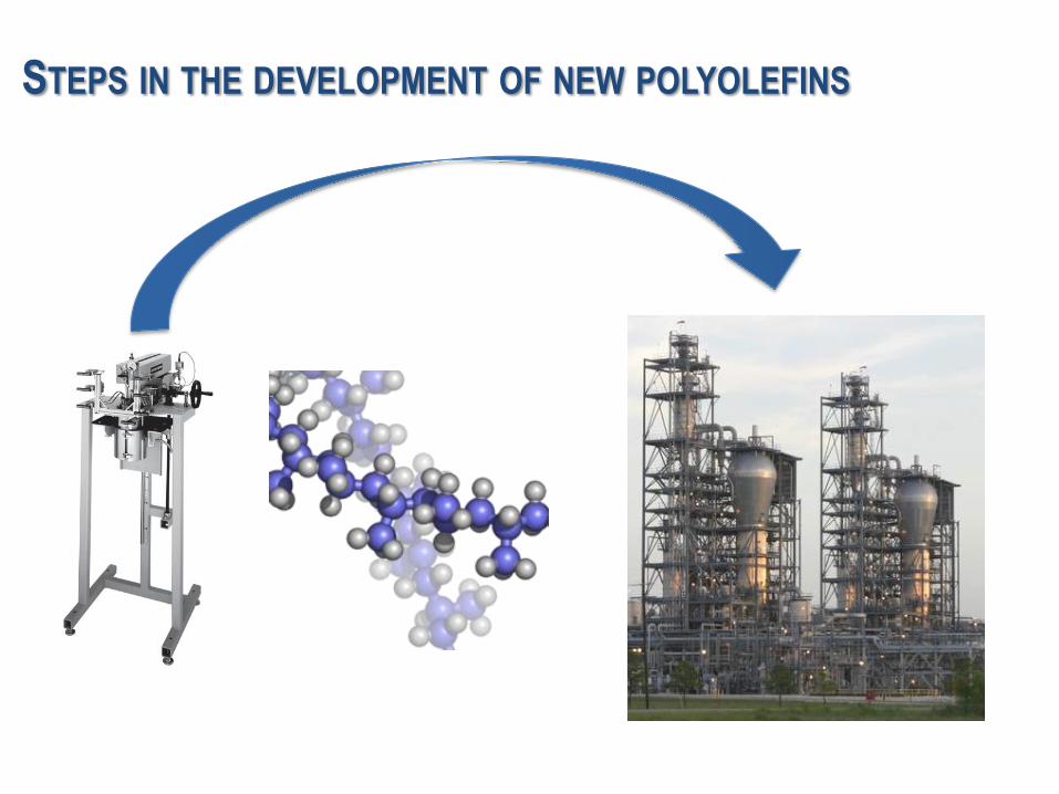
STEPS IN THE DEVELOPMENT OF NEW POLYOLEFINS

0.88

0.910.93

0.950.980

20

40

60

80

100

0.00

1.38

2.7

5

4.13

FA

w(l

ogr

,FA

)

log r

Reactor ↔ Microstructure Models

Microstructure ↔ Property Models

POLYMERIZATION MICROSTRUCTURE PROPERTIES

eth

yle

ne

MFM

a-o

lefin

GCA

TYPICAL REACTOR SYSTEM FOR POLYMERIZATION KINETICS

MEASUREMENT

Generally used for slurry or gas-phase polymerization of ethylene, propylene, and a-olefins.

A reactor calorimeter is the best option to measure liquid bulk propylene polymerization kinetics.

TYPICAL OLEFIN POLYMERIZATION KINETICS CURVES WITH

COORDINATION CATALYSTSM

on

om

er F

low

Rat

e (P

oly

mer

izat

ion

Rat

e)

Polymerization Time

Build-up type

0"

0.1"

0.2"

0.3"

0.4"

0.5"

0.6"

2" 2.5" 3" 3.5" 4" 4.5" 5"

wlog$r$

log$r$

(a) (b)

0.0E+00%

5.0E'05%

1.0E'04%

1.5E'04%

2.0E'04%

0% 10000%20000%30000%40000%50000%60000%

f r!or!w

r$

chain!length!(r)!

fr%

wr%

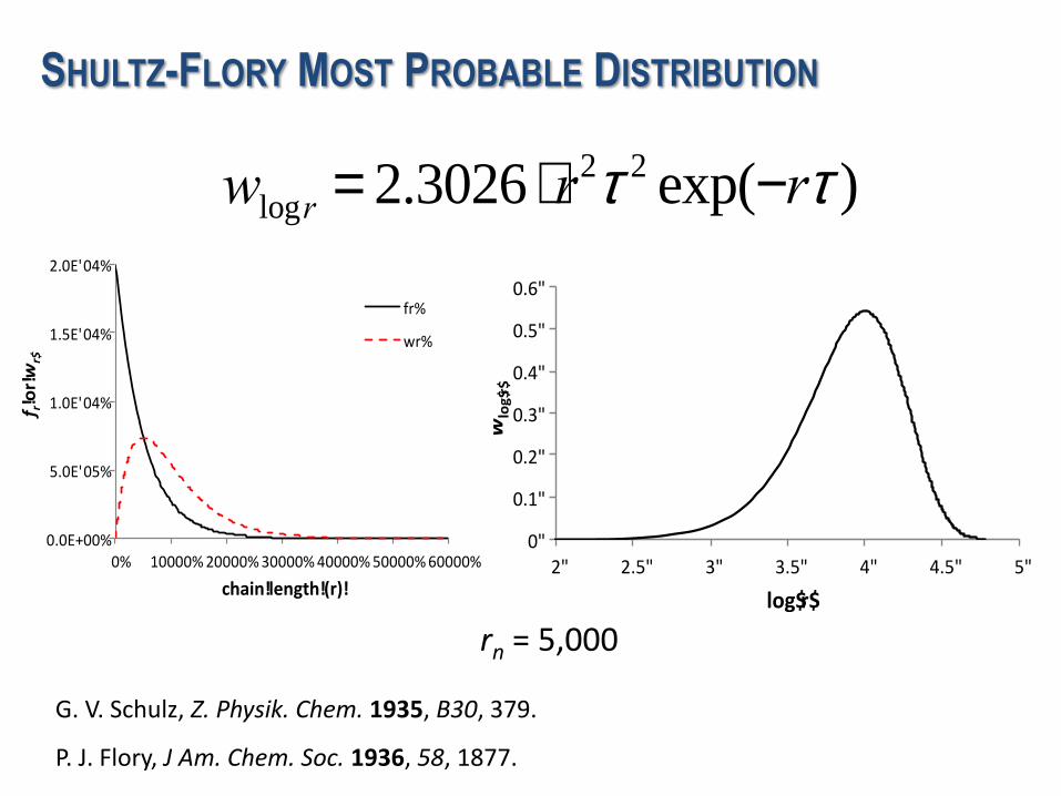
SHULTZ-FLORY MOST PROBABLE DISTRIBUTION

rn = 5,000

G. V. Schulz, Z. Physik. Chem. 1935, B30, 379.

P. J. Flory, J Am. Chem. Soc. 1936, 58, 1877.

wlogr = 2.3026 × r2t 2 exp(-rt )

0.4755&

0.4855&

0.4955&

0.5055&

0.5155&

2.50&

2.75&

3.00&

3.25&

3.50&

3.75&

4.00&

4.25&

4.50&

4.75&

5.00&

F1#

log#r#

(a) (b)

0.4755&0.4855&0.4955&0.5055&0.5155&

0&

20&

40&

60&

80&

100&

120&

2.50&

2.80&

3.10&

3.40&

3.70&

4.00&

4.30&

4.60&

4.90&

F1#

wlogr,F1#

log#r#

0.5

STOCKMAYER BIVARIATE DISTRIBUTION

rn = 5,000, F1 = 0.5 and r1r2 = 1.0:

W. H. Stockmayer, J. Chem. Phys. 1945, 13, 199.

0

10

20

30

40

50

0

0.2

0.4

0.6

0.8

1

2 3 4 5 6 7

SC

B/1

000C

dW

/dlo

gM

W

logMW

Split=50:50

SCB=30SCB=10

0

10

20

30

40

50

0

0.2

0.4

0.6

0.8

1

2 3 4 5 6 7

SC

B/1

000C

dW

/dlo

gM

W

logMW

SCB=20 SCB=20

Split=50:50

0

10

20

30

40

50

0

0.2

0.4

0.6

0.8

1

2 3 4 5 6 7

SC

B/1

000C

dW

/dlo

gM

W

logMW

SCB=10 SCB=30

Split=50:50

CONTROLLING MWD AND CCD

WITH DUAL SINGLE-SITE

CATALYSTS

t = 0 t = tp

log MW

log MW

log MW

log MW

log MW

polymer particle

catalyst particle

SEMI-BATCH POLYMERIZATION

0 50 100 150 200 250 300

E(t

)

Time, min

∞

t = tp = 60 min

≈

log MW

polymer particle

catalyst particle

log MW

log MW

0

0.005

0.01

0.015

0.02

0 50 100 150 200 250 300

E(t

)

Time, min

tR = 60 min

CSTR POLYMERIZATION

1

≈

tr1 ± Dt1 tr2 ± Dt2 tr3 ± Dt3

≅ 0 for large n

tr4 ± Dt4 trn ± Dtn

tR = (tRi ± Dti )i=1

n

å = tRii=1

n

å + (±Dti )i=1

n

å

tr5 ± Dt5

0.00

0.02

0.04

0.06

0 50 100 150 200 250 300

E(t

)

Time, min

1

2

3

10

20

50

∞

≈

CSTR-IN-SERIES POLYMERIZATION

0

4

8

12

16

0 20 40 60

Eth

yle

ne u

pta

ke,

g/m

in

Time, min

C1

C2

C1

C2

0

10

20

30

0

0.4

0.8

1.2

3 4 5 6 7 8

SC

B/1

000C

d W

/d l

og

MW

logMW

CSTR

0

10

20

30

0

0.4

0.8

1.2

3 4 5 6 7 8

SC

B/1

000C

dW

/dlo

gM

W

logMW

Semi-Batch Reactor

SEMI-BATCH TO CSTR SCALE-UP: DIFFERENT KINETICS

0

5

10

15

20

25

30

0

0.2

0.4

0.6

0.8

1

1.2

3 4 5 6 7 8

SC

B/1

000C

d W

/d lo

gM

W

logMW

= 0.511

0

5

10

15

20

25

30

0

0.2

0.4

0.6

0.8

1

1.2

3 4 5 6 7 8

SC

B/1

000C

d W

/d lo

gM

W

logMW

= 0.534

0

5

10

15

20

25

30

0

0.2

0.4

0.6

0.8

1

1.2

3 4 5 6 7 8

SC

B/1

000 C

d W

/d lo

gM

W

logMW

= 0.519

0

5

10

15

20

25

30

0

0.2

0.4

0.6

0.8

1

1.2

3 4 5 6 7 8

SC

B/1

000C

d W

/d l

og

MW

logMW

= 0.762

1 CSTR 2 CSTRs

3 CSTRs 4 CSTRs



0

100000

200000

300000

1 3 5 7 9 11

Mn

Number of CSTRs in series

CSTR

Semi-batch reactor

0

10

20

30

0 20 40 60

Eth

yle

ne u

pta

ke,

g/m

in

Time, min

C1

C2

C1

C2

SEMI-BATCH TO CSTR SCALE-UP: SIMILAR KINETICS

0

10

20

30

0

0.4

0.8

1.2

3 4 5 6 7 8

SC

B/1

000C

d W

/dlo

gM

W

logMW

CSTR

0

10

20

30

0

0.4

0.8

1.2

3 4 5 6 7 8

SC

B/1

000C

dW

/dlo

gM

W

logMW

Semi-Batch Reactor

dLogMdLogM

dw

SCBH

D

1) /(w 1/

ii

0.86

0.88

0.90

0.92

0.94

0.96

0.98

1.00

0.86 0.88 0.90 0.92 0.94 0.96 0.98 1.00

Measured (g/cm3)

Es

tim

ate

d

(g

/cm

3)

Homopolymers

Copolymers

▲ Elastomers

1 to 1 line

+/- 0.002 g/cm3

0

0.05

0.1

0.15

0.2

0.25

0.3

0.35

2 3 4 5 6

Log M

dW

/dL

og

M

Log M slices

SCB/1000TC

Correlations developed from homo &

copolymer samples …

…density on a slice by slice basis added up to

obtain whole polymer density

DENSITY (SLOW COOLED) FROM MWD & SCBD

8

DENSITY (SLOW COOLED) FROM MWD & SCBD

Application to digital Schulz Flory Distributions

MWDs fixed at 2 Density vs. Mw calibration curve calculated SCBD is assumed to be flat Density change with SCB calculated as before All SFD values are additive

dLogMdLogM

dw

SCBH

D

1) /(w 1/

ii

TENSILE VALUES FROM ESTIMATED DENSITIES

Application to digital Schulz Flory Distributions

Tensile values calculated directly from blend density…

1. Density (slow cooled sample)

2. Incorporate the concept of tie molecules

a) Tm (oC) from density

b) Lamella thickness (GT eq.)

c) Probability of tie molecules (PTM )

formation

3. Account for weight fraction effects

(both MWD and SCBD)

Primary Structure Parameter (PSP2)*

ESTIMATING POST YIELD VALUES

*branch type not taken into account

13

Durability of Resin B ~1000x that of A at

the same density (0.950 g/cm3) and MW

0

0.1

0.2

0.3

0.4

0.5

0.6

2 3 4 5 6 7

Log M

dW

/dlo

g M

0

1

2

3

4

5

6

SC

B/1

00

0 T

C

A

0

0.1

0.2

0.3

0.4

0.5

0.6

2 3 4 5 6 7

Log M

dW

/dlo

g M

0

1

2

3

4

5

6

SC

B/1

00

0 T

C

B

~600 NDR

~490 NDR

Calculating PSP2 for SFDs

Data pts – PSP2 values from property model spread sheet for several SFDs

Dotted lines – PSP2 values from above equation calculated from Log Mw and density values

Where:L = PSP2 maxk = PDI constant

(equal to 3.8394 for SFD)x = Log Mw

x mid pt. = mD + c

PSP2 for SFDs can be calculated using a sigmoidal equation

Copolymers = 0.88 g/cm3

Homopolymers

Tensile Test Proxys for Slow Crack Growth Testing

No effect of resin architecture on NDR noted

Large affect of SCB chain type clearly seen in Strain Hardening Modulus (<Gp>, MPa) at 80oC data

PSP2 values being adjusted to reflect difference

Assigned points for copolymers

“Real world” problems are typically very complex, a

true understanding of a system is only possible if many

factors are considered. i.e., multivariable analysis

Chemometric is not a single tool but a range of methods

including:

Basic Statistics

Design of Experiments (DOE)

Multivariable Analysis

Calibration

Curve Fitting

Library Searching

Signal Processing

Principle Component Analysis

Resolution

Detection

Pattern Recognition Methods

Neural Networks

23

Overview of chemometrics as an

investigative tool: Basic concepts

E C6/E H2/E Cat1/Cat2 Temp (oC) Time (min)

1 0.125 0.0289 1.2 60 100

Example RX Conditions

Comparison of products from semi-batch and CSTR reactions: Variables and Responses

DoE (Optimal-IV design; 33 samples) used to compare effects of reactor variables and catalyst types

Min Max

E (mol/L) 0.25 1.5

C6/E 0 0.25

H2/E 0.0075 0.035

Cat1/Cat2 1 20

Temp (oC) 50 80

Time (min) 30 120

Digital bimodal structures generated from reactor models

Differences in blend component attributes (Mw, SCB and wt. fractions) evaluated via pattern recognition methods

Rx Ranges (six factors)

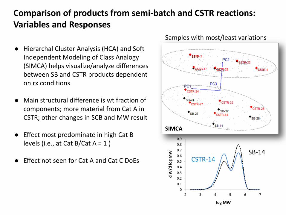
Hierarchal Cluster Analysis (HCA) and Soft Independent Modeling of Class Analogy (SIMCA) helps visualize/analyze differences between SB and CSTR products dependent on rx conditions

Main structural difference is wt fraction of components; more material from Cat A in CSTR; other changes in SCB and MW result

Effect most predominate in high Cat B levels (i.e., at Cat B/Cat A = 1 )

Effect not seen for Cat A and Cat C DoEs

Samples with most/least variations

CSTR-14SB-14

SIMCA

Comparison of products from semi-batch and CSTR reactions: Variables and Responses

Comparison of products from semi-batch and CSTR reactions: Interpretations

• If the shape of polymerization kinetics profiles of the single-site catalysts is different, then we can expect that the MWD x SCB profiles of polymers made in semi-batch reactors and CSTRs will differ because polymer particles exiting the CSTR will have a different split from those of polymer particles staying exactly the same time in the semi-batch reactor.

Assumption: DoE polynomial models can adequately reproduce complex rx and property models

A six factor Optimal-IV design was used to generate a digital, fifth order DoE (497 samples) to test proof of concept

Response variables modeled from rx input

Each response variable modeled independently & response variable error assigned to replicate samples

Example of x5 DoE rx response space

Using DoE for predictive modeling: Choice of DoE and Model Validation

A IV-optimal design seeks to minimize the integral of the prediction variance across the design space. These designs are built algorithmically to provide lower prediction variance across the entire design space.

Results for Catalyst B

Excellent fits obtained for all response variables (i.e., predicted RSQ between 0.9985 and 1 for primary responses; 0.9885 to 0.9997 for derivative responses)

Validation DoE runs (off axis rx conditions not included in DoE model) show excellent agreement with spread sheet calculations

Expected structural outcomes seen with changes in rx conditions as well as expected trends between responses; e.g., decrease in PSP2 as density increases

Well covered rx space does not translate into well covered space for responses

Design-Expert® Software

Blend density

Color points by value of

Blend density:

0.967885

0.89479

Actual

Pre

dic

ted

Predicted vs. Actual

0.88

0.90

0.92

0.94

0.96

0.98

0.88 0.90 0.92 0.94 0.96 0.98


Correlation: -0.858

Color points by

Run

471

1

Blend PSP2

Ble

nd

de

ns

ity

0 5 10 15 20 25 30

0.88

0.9

0.92

0.94

0.96

0.98

Blend Density (g/cm3)Adj RSQ = 0.9944Pred RSQ = 0.9885

Do

E P

red

.

Kinetic and Property Models Pred.

Ble

nd

De

nsi

ty

Blend PSP2


Response spaces from Optimal-IV fifth ordered DoE from Cat B

However, even in areas with no response data , e.g., C1 Mw ~ 110 kg/mol, C2 Mw ~ 900 kg/mol, excellent predictive values are give by DoE model, moreover rx conditions needed to achieve the MW were obtained via reverse models

Region with no response data


Use of Reverse Models

Rx dataDoE

SpacePossible products

Screening Process One advantage of using DoE models is the ability to determine the conditions required to make polymers with targeted properties using response space

In these studies the optimization function provided in the DoE software (StatEasev8.03) was used for testing this concept

Method can be used to help validate response space

For predictive use, samples should be taken from validated space

Selected resin structure and rx variables may need to be held constant to reduce multiple solutions

Example of Target Resin

Example of Reverse Model Solution

Rx Input (one solution results from set variables and structural targets)

DoE Model Prediction Stats

= Fixed VarE C6/E H2/E Cat2/Cat1 Temp Time

0.68 0.062 0.009933 0.98 62.51 32.1

C1 Mw is target = 110000

C2 Mw is target = 900000

Wt Frac C1 is target = 0.5

Blend Mw is target = 503400

Structural targets used as input at fixed rx variables

Assumption: Results from a higher order DoE can be adequately represented using a lower order DoE

Concept evaluated using a digital six factor, second order DoE (33 samples with five replicates)

Excellent to good fits were obtained for both primary and derivative responses

Second order models with up to six factors can be used to navigate design space and investigate relationships

Validation runs help decide if augmentation of lower order design is needed, depends on use of data

Comparison of DoE response spaces


yellow pts = x5 DoE; black pts = x2 DoE

Validation and Augmentation Strategies Focused on most influential rx variables (use

DoE ANOVA results) and primary responses, looked for gaps

Use DoE software reverse models to suggest initial rx values that fill gaps,

Constructed small DoEs to generate data for the desired space if needed. Run samples and include results if warranted

Repeat process until acceptable error is established

Additional Validation DoEs constructed and tested (29 and 11 additional runs)

Original data set augmented (6 samples) All predicted values from validation samples fell

with in 95% Predictive Limits Relative error of predicted value deemed

acceptable (< 10%)

For Second Order Digital DoE

Experimental DoE

Digital studies were followed up with an experimental solution polymerization study

Evaluated a five factor second order DoE (33 samples with five replicates)

Similar variable responses used as before, C1 & C2 values found by fitting MWDs with SFDs

Validation/augmentation runs will be conducted as described in second order digital DoE

Rx Ranges (five factors)

Initial results from experimental design

Mixed results for fits Lower predictive fits to C1 Mw may be

caused by small range of variation (~13% vs 39% for C2)

Good fits for SCB content, Wt Frac C1 and Blend data


Factor Coding: Actual

Original Scale

Blend Mw

172721

22622

X1 = A: CE

X2 = B: C6/CE

Actual Factors

C: CAT/CAT2 = 1.67

D: Temp = 129.19

E: Time = 5.89

0.00

0.20

0.40

0.60

0.80

0.20

0.34

0.47

0.61

0.75

19196

32472

45747

59023

72298

85574

B

len

d M

w

A: CE B: C6/CE

Expected main effects on response variables (e.g.) All four factors for Mw, effects of C6 on Mw

clearly seen E & C6 for SCB levels E, Cat2/Cat 1 ratio, and time for Wt Frac C1

Physical and mechanical testing of samples under way; property estimates will be done once refined SCB data is obtained

Summary Kinetic and property models give us insight of how catalyst and reactor

variables can be manipulated to give desired PE bimodal products

Semi batch and CSTR can produce significantly different products for some catalyst pairs

Mapping the structure-property space of bimodal polyethylene can be accomplished by adequately reproducing complex rx and property models through the appropriate DoE model, both forward and reverse models

Reverse models require several variables to be held constant to reduce multiple solutions

Digital data shows that higher order DoE can be adequately represented using a lower order DoEs if appropriate validation and augmentation efforts are made

Current efforts to use these methods for experimentally solution based polymerization products are currently underway

Acknowledgments

• NSERC Canada Research Chair Program

• Chevron Phillips Chemical Company, LP

6th International Conference

on Polyolefin Characterization

& Short Course on Separation Techniques for Polyolefins

November 6-9, 2016. Shanghai, China.

mapping the structure-property s bimodal … an… · mapping the structure-property space of...

Documents