mahler measures,short walksand log-sine integrals · 2011-06-02 · 3. introduction 16. short...
TRANSCRIPT
3. Introduction16. Short Random Walks
40. Multiple Mahler Measures47. Log-sine Integrals
Mahler Measures, Short Walks andLog-sine Integrals
A case study in hybrid computation
Jonathan M. Borwein frsc faa faaas
Laureate Professor & Director of CARMA, Univ. of Newcastlethis talk: http://carma.newcastle.edu.au/jon/handbook.pdf
SNC 2011San Jose, June 7-9, 2011
Revised: June 2, 2011issac paper: http://carma.newcastle.edu.au/jon/logsin3.pdf
J.M. Borwein Mahler Measures

3. Introduction16. Short Random Walks
40. Multiple Mahler Measures47. Log-sine Integrals
Contents. We will cover some of the following:
1 3. Introduction7. Multiple Polylogarithms8. Log-sine Integrals9. Random Walks14. Mahler Measures15. Carlson’s Theorem
2 16. Short Random Walks17. Combinatorics23. Meijer-G functions28. Hypergeometric values of W3,W431. Probability and Bessel J39. Derivative values of W3,W4
3 40. Multiple Mahler Measures41. Relations to η42. Smyth’s results revisited44. Boyd’s Conjectures46. A Bonus Measure
4 47. Log-sine Integrals47. Sasaki’s Mahler Measures50. Log-sine-cosine integrals55. Three Cognate Evaluations57. KLO’s Mahler Measures61. Conclusion
J.M. Borwein Mahler Measures

3. Introduction16. Short Random Walks
40. Multiple Mahler Measures47. Log-sine Integrals
The world is hybrid
Program Committee Lihong Zhi, Chair Academy of Mathematics and Systems Science, China
Daniel Bates Colorado State University, USA
Mark Giesbrecht University of Waterloo, Canada
Stef Graillat Université Pierre et Marie Curie, France
Claude-Pierre Jeannerod INRIA (LIP ENS Lyon), Lyon, France
Hiroshi Kai Ehime University, Japan
Erich Kaltofen North Carolina State University, USA
Bingyu Li Northeast Normal University, China
Teo Mora University of Genova, Italy
Bernard Mourrain INRIA Sophia Antipolis, France
Kosaku Nagasaka Kobe University, Japan
Victor Pan City University of New York, USA
Greg Reid The University of Western Ontario, Canada
Kiyoshi Shirayanagi Toho University, Japan
Franz Winkler Johannes Kepler University, Austria
Organizing Committee General ChairIlias Kotsireas Waterloo, Canada Program Committee Chair Lihong Zhi Beijing, China Treasurer Werner Krandick Philadelphia, USA
Publicity Chair Erik Postma Maplesoft, Canada Webmaster Guillaume Moroz Nancy, France June 7-9, 2011, San Jose, California
The 4th international workshop on Symbolic-Numeric Computation
http://www.cargo.wlu.ca/SNC2011/
Invited Speakers
Laureate Professor Jonathan BorweinUniversity of Newcastle,Australia.
Professor James DemmelUC Berkeley,United States of America.
Professor Stephen WattUniversity of Western Ontario,Canada.
J.M. Borwein Mahler Measures

3. Introduction16. Short Random Walks
40. Multiple Mahler Measures47. Log-sine Integrals
8. Multiple Polylogarithms9. Log-sine Integrals10. Random Walks15. Mahler Measures16. Carlson’s Theorem
Congrats to NIST: for helping answer eternal questions
Special Functions in the 21st Century:
Theory & Applications April 6–8, 2011Washington, DC
Objectives. The conference will provide a forum for the exchange of expertise, experience and insights among world leaders in the subject of special functions. Participants will include expert authors, editors and validators of the recently published NIST Handbook of Mathematical Functions and Digital Library of Mathematical Functions (DLMF). It will also provide an opportunity for DLMF users to interact with its creators and to explore potential areas of fruitful future developments.
F.W.J. Olver
Special Recognition of Professor Frank W. J. Olver. This conference is dedicated to Professor Olver in light of his seminal con-tributions to the advancement of special functions, especially in the area of asymptotic analysis and as Mathematics Editor of the DLMF.
Plenary Speakers Richard Askey, University of Wisconsin Michael Berry, University of Bristol Nalini Joshi, University of Sydney, Australia Leonard Maximon, George Washington University William Reinhardt, University of Washington Roderick Wong, City University of Hong Kong
Call for Contributed Talks (25 Minutes) Abstracts may be submitted to [email protected] until March 15, 2011.
Registration and Financial Assistance. Registration fee: $120. Courtesy of SIAM, limited travel support is available for US-based postdoc and early career researchers. Courtesy of City University of Hong Kong and NIST, partial support is available for others in cases of need. Submit all requests for financial assistance to [email protected].
Venue. Renaissance Washington Dupont Circle Hotel, 1143 New Hampshire Avenue NW, Washington, DC, 20037 USA. The conference rate is $259, available until March 15. Refreshments are supplied courtesy of University of Maryland.
Organizing Committee. Daniel Lozier, NIST, Gaithersburg, Maryland; Adri Olde Daalhuis, Univer-sity of Edinburgh; Nico Temme, CWI, Amsterdam; Roderick Wong, City University of Hong Kong
To register online for the conference, and reserve a room at the conference hotel, see http://math.nist.gov/~DLozier/SF21
J.M. Borwein Mahler Measures

3. Introduction16. Short Random Walks
40. Multiple Mahler Measures47. Log-sine Integrals
8. Multiple Polylogarithms9. Log-sine Integrals10. Random Walks15. Mahler Measures16. Carlson’s Theorem
Abstract toc
• The Mahler measure of a polynomial of several variables hasbeen a subject of much study over the past thirty years.
• Very few closed forms are proven but more are conjectured.
• We provide systematic evaluations of various higher andmultiple Mahler measures using moments of random walksand values of log-sine integrals.
• We also explore related generating functions for the log-sineintegrals and their generalizations.
• This work would be impossible without very extensive symbolicand numeric computations. It also makes frequent use of thenew NIST Handbook of Mathematical Functions.
My intention is to show off the interplay between numeric andsymbolic computing while exploring the three topics in title.
J.M. Borwein Mahler Measures

3. Introduction16. Short Random Walks
40. Multiple Mahler Measures47. Log-sine Integrals
8. Multiple Polylogarithms9. Log-sine Integrals10. Random Walks15. Mahler Measures16. Carlson’s Theorem
.
J.M. Borwein Mahler Measures

3. Introduction16. Short Random Walks
40. Multiple Mahler Measures47. Log-sine Integrals
8. Multiple Polylogarithms9. Log-sine Integrals10. Random Walks15. Mahler Measures16. Carlson’s Theorem
Other References
1 Joint with: Armin Straub (Tulane) and James Wan (UofN)- and variously with: David Bailey (LBNL), David Borwein
(UWO), Dirk Nuyens (Leuven), Wadim Zudilin (UofN).
2 Most results are written up in FPSAC 2010, ISSAC 2011(JB-AS: best student paper),RAMA, Exp. Math, J. AustMS,Can. Math J. . See:
• www.carma.newcastle.edu.au/~jb616/walks.pdf• www.carma.newcastle.edu.au/~jb616/walks2.pdf• www.carma.newcastle.edu.au/~jb616/densities.pdf• www.carma.newcastle.edu.au/~jb616/logsin.pdf• www.carma.newcastle.edu.au/~jb616/logsin2.pdf.• http://carma.newcastle.edu.au/jon/logsin3.pdf
3 This and related talks are housed at www.carma.newcastle.edu.au/~jb616/papers.html#TALKS
J.M. Borwein Mahler Measures

3. Introduction16. Short Random Walks
40. Multiple Mahler Measures47. Log-sine Integrals
8. Multiple Polylogarithms9. Log-sine Integrals10. Random Walks15. Mahler Measures16. Carlson’s Theorem
My Collaborators
J.M. Borwein Mahler Measures

3. Introduction16. Short Random Walks
40. Multiple Mahler Measures47. Log-sine Integrals
8. Multiple Polylogarithms9. Log-sine Integrals10. Random Walks15. Mahler Measures16. Carlson’s Theorem
Multiple Polylogarithms:
Lia1,...,ak(z) :=∑
n1>···>nk>0
zn1
na11 · · ·nakk
.
Thus, Li2,1(z) =∑∞
k=1zk
k2∑k−1
j=11j . Specializing produces:
• The polylogarithm of order k: Lik(x) =∑∞
n=1xn
nk.
• Multiple zeta values:
ζ(a1, . . . , ak) := Lia1,...,ak(1).
• Multiple Clausen (Cl) and Glaisher functions (Gl) of depth kand weight w :=
∑aj :
Cla1,...,ak (θ) :=
{Im Lia1,...,ak(eiθ) if w evenRe Lia1,...,ak(eiθ) if w odd
},
Gla1,...,ak (θ) :=
{Re Lia1,...,ak(eiθ) if w evenIm Lia1,...,ak(eiθ) if w odd
}.
J.M. Borwein Mahler Measures

3. Introduction16. Short Random Walks
40. Multiple Mahler Measures47. Log-sine Integrals
8. Multiple Polylogarithms9. Log-sine Integrals10. Random Walks15. Mahler Measures16. Carlson’s Theorem
Log-sine Integrals
The log-sine integrals are defined for n = 1, 2, . . . by
Lsn (σ) := −∫ σ
0logn−1
∣∣∣∣2 sinθ
2
∣∣∣∣ dθ (1)
and their moments for k ≥ 0 given by
Ls(k)n (σ) := −
∫ σ
0θk logn−1−k
∣∣∣∣2 sinθ
2
∣∣∣∣ dθ. (2)
• Ls1 (σ) = −σ and Ls(0)n (σ) = Lsn (σ), as in Lewin. In
particular,
Ls2 (σ) = Cl2 (σ) :=
∞∑n=1
sin(nσ)
n2(3)
is the Clausen function which plays a prominent role.
J.M. Borwein Mahler Measures

3. Introduction16. Short Random Walks
40. Multiple Mahler Measures47. Log-sine Integrals
8. Multiple Polylogarithms9. Log-sine Integrals10. Random Walks15. Mahler Measures16. Carlson’s Theorem
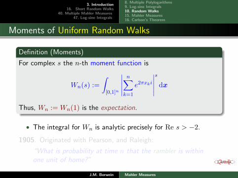
Moments of Uniform Random Walks
Definition (Moments)
For complex s the n-th moment function is
Wn(s) :=
∫[0,1]n
∣∣∣∣∣n∑k=1
e2πxki
∣∣∣∣∣s
dx
Thus, Wn := Wn(1) is the expectation.
• The integral for Wn is analytic precisely for Re s > −2.
1905. Originated with Pearson, and Raleigh:
“What is probability at time n that the rambler is withinone unit of home?”
J.M. Borwein Mahler Measures
3. Introduction16. Short Random Walks
40. Multiple Mahler Measures47. Log-sine Integrals
8. Multiple Polylogarithms9. Log-sine Integrals10. Random Walks15. Mahler Measures16. Carlson’s Theorem
Moments of Uniform Random Walks
Definition (Moments)
For complex s the n-th moment function is
Wn(s) :=
∫[0,1]n
∣∣∣∣∣n∑k=1
e2πxki
∣∣∣∣∣s
dx
Thus, Wn := Wn(1) is the expectation.
• The integral for Wn is analytic precisely for Re s > −2.
1905. Originated with Pearson, and Raleigh:
“What is probability at time n that the rambler is withinone unit of home?”
J.M. Borwein Mahler Measures

3. Introduction16. Short Random Walks
40. Multiple Mahler Measures47. Log-sine Integrals
8. Multiple Polylogarithms9. Log-sine Integrals10. Random Walks15. Mahler Measures16. Carlson’s Theorem
Clearly W1 = 1. What about W2(1)?
W2 =
∫ 1
0
∫ 1
0
∣∣e2πix + e2πiy∣∣ dxdy = ?
– Mathematica 7 and Maple 14 think the answer is 0.
• There is always a 1-dimension reduction
Wn(s) =
∫[0,1]n
∣∣∣∣ n∑k=1
e2πxki
∣∣∣∣sdx=
∫[0,1]n−1
∣∣∣∣1 +n−1∑k=1
e2πxki
∣∣∣∣sd(x1, . . . , xn−1)
• So
W2 = 4
∫ 1/4
0cos(πx) dx =
4
π.
J.M. Borwein Mahler Measures

3. Introduction16. Short Random Walks
40. Multiple Mahler Measures47. Log-sine Integrals
8. Multiple Polylogarithms9. Log-sine Integrals10. Random Walks15. Mahler Measures16. Carlson’s Theorem
Clearly W1 = 1. What about W2(1)?
W2 =
∫ 1
0
∫ 1
0
∣∣e2πix + e2πiy∣∣ dxdy = ?
– Mathematica 7 and Maple 14 think the answer is 0.
• There is always a 1-dimension reduction
Wn(s) =
∫[0,1]n
∣∣∣∣ n∑k=1
e2πxki
∣∣∣∣sdx=
∫[0,1]n−1
∣∣∣∣1 +
n−1∑k=1
e2πxki
∣∣∣∣sd(x1, . . . , xn−1)
• So
W2 = 4
∫ 1/4
0cos(πx) dx =
4
π.
J.M. Borwein Mahler Measures

3. Introduction16. Short Random Walks
40. Multiple Mahler Measures47. Log-sine Integrals
8. Multiple Polylogarithms9. Log-sine Integrals10. Random Walks15. Mahler Measures16. Carlson’s Theorem
n ≥ 3 highly nontrivial and n ≥ 5 not well understood.
• Similar problems get much more difficult in five or moredimensions — e.g., Bessel moments, Box integrals, Isingintegrals (work with Bailey, Broadhurst, Crandall, ...).
- In fact, W5 ≈ 2.0081618 was the best estimate we couldcompute directly, on 256 cores at Lawrence Berkeley NationalLaboratory.
- Bailey and I have a general project to develop symbolicnumeric techniques for (meaningful) multi-dim integrals.
When the facts change, I change my mind. What do you do, sir?— John Maynard Keynes in Economist Dec 18, 1999.
J.M. Borwein Mahler Measures

3. Introduction16. Short Random Walks
40. Multiple Mahler Measures47. Log-sine Integrals
8. Multiple Polylogarithms9. Log-sine Integrals10. Random Walks15. Mahler Measures16. Carlson’s Theorem
One 1500-step Ramble: a familiar picture
2D and 3D lattice walks are
different:
A drunk man willfind his wayhome but adrunk bird mayget lost forever.— ShizuoKakutani
• 1D (and 3D) easy. Expectation of RMS distance is easy (√n).
• 1D or 2D lattice: probability one of returning to the origin.
J.M. Borwein Mahler Measures

3. Introduction16. Short Random Walks
40. Multiple Mahler Measures47. Log-sine Integrals
8. Multiple Polylogarithms9. Log-sine Integrals10. Random Walks15. Mahler Measures16. Carlson’s Theorem
1000 three-step Rambles: a less familiar picture?
J.M. Borwein Mahler Measures

3. Introduction16. Short Random Walks
40. Multiple Mahler Measures47. Log-sine Integrals
8. Multiple Polylogarithms9. Log-sine Integrals10. Random Walks15. Mahler Measures16. Carlson’s Theorem
Mahler Measures (1923) in several variables
The logarithmic Mahler measure of a (Laurent) polynomial P :
µ(P ) :=
∫ 1
0
∫ 1
0· · ·∫ 1
0log |P
(e2πiθ1 , · · · , e2πiθn
)| dθ1 · · · dθn.
• M1 := P 7→ exp(µ(P )) is multiplicative.• n = 1: P is a product of cyclotomics ⇔M1(P ) = 1.
Lehmer’s conjecture (1931) is: otherwiseM1(P ) ≥M1(1− x+ x3 − x4 + x5 − x6 + x7 − x9 + x10).
• µ(P ) turns out to be an example of a period.• When n = 1 and P has integer coefficients M1(P ) is an
algebraic integer.• In several dimensions life is harder.
- We shall see remarkable recent results — many morediscovered than proven — expressing µ(P ) arithmetically.
J.M. Borwein Mahler Measures

3. Introduction16. Short Random Walks
40. Multiple Mahler Measures47. Log-sine Integrals
8. Multiple Polylogarithms9. Log-sine Integrals10. Random Walks15. Mahler Measures16. Carlson’s Theorem
Carlson’s Theorem: from discrete to continuous
Theorem (Carlson (1914, PhD) )
If f(z) is analytic for Re (z) ≥ 0, its growth on the imaginary axisis bounded by ecy, |c| < π, and
0 = f(0) = f(1) = f(2) = . . .
then f(z) = 0 identically.
• sin(πz) does not satisfy the conditions of the theorem, as itgrows like eπy on the imaginary axis.
• Wn(s) satisfies the conditions of the theorem (and is in factanalytic for Re (s) > −2 when n > 2).
• There is a lovely 1941 proof by Selberg of the bounded case.• The theorem lies under much of what follows.
J.M. Borwein Mahler Measures

3. Introduction16. Short Random Walks
40. Multiple Mahler Measures47. Log-sine Integrals
18. Combinatorics24. Meijer-G functions29. Hypergeometric values of W3,W432. Probability and Bessel J40. Derivative values of W3,W4
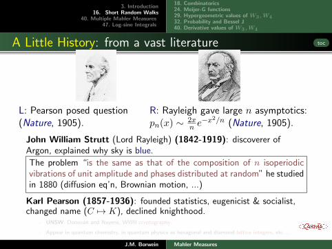
A Little History: from a vast literature toc
L: Pearson posed question(Nature, 1905).
R: Rayleigh gave large n asymptotics:pn(x) ∼ 2x
n e−x2/n (Nature, 1905).
John William Strutt (Lord Rayleigh) (1842-1919): discoverer ofArgon, explained why sky is blue.
The problem “is the same as that of the composition of n isoperiodicvibrations of unit amplitude and phases distributed at random” he studiedin 1880 (diffusion eq’n, Brownian motion, ...)
Karl Pearson (1857-1936): founded statistics, eugenicist & socialist,changed name (C 7→ K), declined knighthood.
- UNSW: Donovan and Nuyens, WWII cryptography.
- Appear in quantum chemistry, in quantum physics as hexagonal and diamond lattice integers, etc ...
J.M. Borwein Mahler Measures

3. Introduction16. Short Random Walks
40. Multiple Mahler Measures47. Log-sine Integrals
18. Combinatorics24. Meijer-G functions29. Hypergeometric values of W3,W432. Probability and Bessel J40. Derivative values of W3,W4
A Little History: from a vast literature toc
L: Pearson posed question(Nature, 1905).
R: Rayleigh gave large n asymptotics:pn(x) ∼ 2x
n e−x2/n (Nature, 1905).
John William Strutt (Lord Rayleigh) (1842-1919): discoverer ofArgon, explained why sky is blue.
The problem “is the same as that of the composition of n isoperiodicvibrations of unit amplitude and phases distributed at random” he studiedin 1880 (diffusion eq’n, Brownian motion, ...)
Karl Pearson (1857-1936): founded statistics, eugenicist & socialist,changed name (C 7→ K), declined knighthood.
- UNSW: Donovan and Nuyens, WWII cryptography.
- Appear in quantum chemistry, in quantum physics as hexagonal and diamond lattice integers, etc ...
J.M. Borwein Mahler Measures

3. Introduction16. Short Random Walks
40. Multiple Mahler Measures47. Log-sine Integrals
18. Combinatorics24. Meijer-G functions29. Hypergeometric values of W3,W432. Probability and Bessel J40. Derivative values of W3,W4
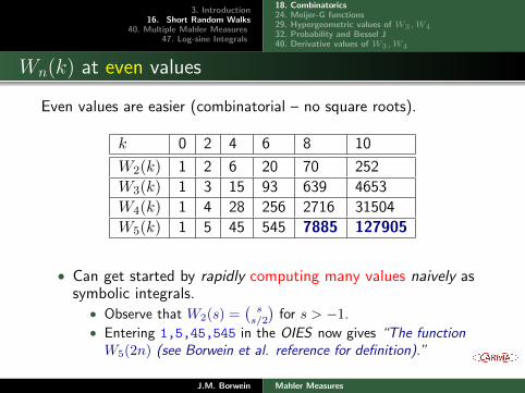
Wn(k) at even values
Even values are easier (combinatorial – no square roots).
k 0 2 4 6 8 10
W2(k) 1 2 6 20 70 252
W3(k) 1 3 15 93 639 4653
W4(k) 1 4 28 256 2716 31504
W5(k) 1 5 45 545 7885 127905
• Can get started by rapidly computing many values naively assymbolic integrals.
• Observe that W2(s) =(ss/2
)for s > −1.
• Entering 1,5,45,545 in the OIES now gives “The functionW5(2n) (see Borwein et al. reference for definition).”
J.M. Borwein Mahler Measures

3. Introduction16. Short Random Walks
40. Multiple Mahler Measures47. Log-sine Integrals
18. Combinatorics24. Meijer-G functions29. Hypergeometric values of W3,W432. Probability and Bessel J40. Derivative values of W3,W4
Wn(k) at even values
Even values are easier (combinatorial – no square roots).
k 0 2 4 6 8 10
W2(k) 1 2 6 20 70 252
W3(k) 1 3 15 93 639 4653
W4(k) 1 4 28 256 2716 31504
W5(k) 1 5 45 545 7885 127905
• Can get started by rapidly computing many values naively assymbolic integrals.
• Observe that W2(s) =(ss/2
)for s > −1.
• Entering 1,5,45,545 in the OIES now gives “The functionW5(2n) (see Borwein et al. reference for definition).”
J.M. Borwein Mahler Measures

3. Introduction16. Short Random Walks
40. Multiple Mahler Measures47. Log-sine Integrals
18. Combinatorics24. Meijer-G functions29. Hypergeometric values of W3,W432. Probability and Bessel J40. Derivative values of W3,W4
Wn(k) at odd integers
n k = 1 k = 3 k = 5 k = 7 k = 9
2 1.27324 3.39531 10.8650 37.2514 132.449
3 1.57460 6.45168 36.7052 241.544 1714.62
4 1.79909 10.1207 82.6515 822.273 9169.625 2.00816 14.2896 152.316 2037.14 31393.1
6 2.19386 18.9133 248.759 4186.19 82718.9
Please, memorize this number!During the three years which I spent at Cambridge my time was wasted, as far as the academical studies were
concerned, as completely as at Edinburgh and at school. I attempted mathematics, and even went during the
summer of 1828 with a private tutor (a very dull man) to Barmouth, but I got on very slowly. The work was
repugnant to me, chiefly from my not being able to see any meaning in the early steps in algebra. This impatience
was very foolish, and in after years I have deeply regretted that I did not proceed far enough at least to understand
something of the great leading principles of mathematics, for men thus endowed seem to have an extra sense. —
Autobiography of Charles Darwin
J.M. Borwein Mahler Measures

3. Introduction16. Short Random Walks
40. Multiple Mahler Measures47. Log-sine Integrals
18. Combinatorics24. Meijer-G functions29. Hypergeometric values of W3,W432. Probability and Bessel J40. Derivative values of W3,W4
Resolution at even values
• General even formula counts n-letter abelian squares xπ(x) oflength 2k.
– Shallit and Richmond (2008) give asymptotics:
Wn(2k) =∑
a1+...+an=k
(k
a1, ..., an
)2
. (4)
• Known to satisfy convolutions:
Wn1+n2(2k) =
k∑j=0
(k
j
)2
Wn1(2j)Wn2(2(k − j)).
• Has recursions such as:
(k + 2)2W3(2k + 4)− (10k2 + 30k + 23)W3(2k + 2)
+9(k + 1)2W3(2k) = 0.
J.M. Borwein Mahler Measures

3. Introduction16. Short Random Walks
40. Multiple Mahler Measures47. Log-sine Integrals
18. Combinatorics24. Meijer-G functions29. Hypergeometric values of W3,W432. Probability and Bessel J40. Derivative values of W3,W4
Analytic continuation: From Carlson’s Theorem
• So integer recurrences yield complex functional equations. Viz
(s+4)2W3(s+4)−2(5s2+30s+46)W3(s+2)+9(s+2)2W3(s) = 0.
• This gives analytic continuations of the ramble integrals tothe complex plane, with poles at certain negative integers(likewise for all n).
– W3(s) has a simple pole at −2 with residue 2√3π, and other
simple poles at −2k with residues a rational multiple of Res−2.
“For it is easier to supply the proof when we have previously acquired, by
the method [of mechanical theorems], some knowledge of the questions
than it is to find it without any previous knowledge. — Archimedes.
J.M. Borwein Mahler Measures

3. Introduction16. Short Random Walks
40. Multiple Mahler Measures47. Log-sine Integrals
18. Combinatorics24. Meijer-G functions29. Hypergeometric values of W3,W432. Probability and Bessel J40. Derivative values of W3,W4
Odd dimensions look like 3
W3(s) on [−6, 52 ]
• JW proved zeroes near to but not at integers: W3(−2n− 1) ↓ 0.J.M. Borwein Mahler Measures

3. Introduction16. Short Random Walks
40. Multiple Mahler Measures47. Log-sine Integrals
18. Combinatorics24. Meijer-G functions29. Hypergeometric values of W3,W432. Probability and Bessel J40. Derivative values of W3,W4
Some even dimensions look more like 4
L: W4(s) on [−6, 1/2]. R: W5 on [−6, 2] (T), W6 on [−6, 2] (B).
• The functional equation (with double poles) for n = 4 is
(s+ 4)3W4(s+ 4) − 4(s+ 3)(5s2 + 30s+ 48)W4(s+ 2)
+ 64(s+ 2)3W4(s) = 0
• There are (infinitely many) multiple poles if and only if 4|n.• Why is W4 positive on R?
J.M. Borwein Mahler Measures

3. Introduction16. Short Random Walks
40. Multiple Mahler Measures47. Log-sine Integrals
18. Combinatorics24. Meijer-G functions29. Hypergeometric values of W3,W432. Probability and Bessel J40. Derivative values of W3,W4
Meijer-G functions (1936– )
Definition
Gm,np,q
(a1, . . . , apb1, . . . , bq
∣∣∣∣x) :=1
2πi×
∫L
∏mj=1 Γ(bj − s)
∏nj=1 Γ(1− aj + s)∏p
j=n+1 Γ(aj − s)∏qj=m+1 Γ(1− bj + s)
xsds.
• Contour L lies between poles of Γ(1−ai− s) and of Γ(bi + s).
- A broad generalization of hypergeometric functions —capturing Bessel Y,K and much more.
- Important in CAS — if better hidden; often lead tosuperpositions of generalized hypergeometric terms pFq.
J.M. Borwein Mahler Measures

3. Introduction16. Short Random Walks
40. Multiple Mahler Measures47. Log-sine Integrals
18. Combinatorics24. Meijer-G functions29. Hypergeometric values of W3,W432. Probability and Bessel J40. Derivative values of W3,W4
Meijer-G forms for W3
Theorem (Meijer form for W3)
For s not an odd integer
W3(s) =Γ(1 + s
2)√π Γ(− s
2)G21
33
(1, 1, 1
12 ,−
s2 ,−
s2
∣∣∣∣14).
• First found by Crandall via CAS.• Proved using residue calculus methods.• W3(s) is among few non-trivial Meijer-G with a closed form.
The most important aspect in solving a mathematical problem is the
conviction of what is the true result. Then it took 2 or 3 years using
the techniques that had been developed during the past 20 years or so.
— Lennart Carleson (From 1966 IMU address on his positive solution of
Luzin’s problem).J.M. Borwein Mahler Measures

3. Introduction16. Short Random Walks
40. Multiple Mahler Measures47. Log-sine Integrals
18. Combinatorics24. Meijer-G functions29. Hypergeometric values of W3,W432. Probability and Bessel J40. Derivative values of W3,W4
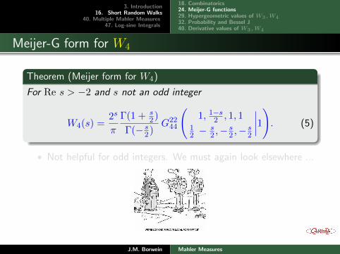
Meijer-G form for W4
Theorem (Meijer form for W4)
For Re s > −2 and s not an odd integer
W4(s) =2s
π
Γ(1 + s2)
Γ(− s2)
G2244
(1, 1−s
2 , 1, 112 −
s2 ,−
s2 ,−
s2
∣∣∣∣1). (5)
• Not helpful for odd integers. We must again look elsewhere ...
He [Gauss(or Mma)] is like the fox, who effaces his tracks in the sand with his tail.— Niels Abel (1802-1829)J.M. Borwein Mahler Measures
3. Introduction16. Short Random Walks
40. Multiple Mahler Measures47. Log-sine Integrals
18. Combinatorics24. Meijer-G functions29. Hypergeometric values of W3,W432. Probability and Bessel J40. Derivative values of W3,W4
Meijer-G form for W4
Theorem (Meijer form for W4)
For Re s > −2 and s not an odd integer
W4(s) =2s
π
Γ(1 + s2)
Γ(− s2)
G2244
(1, 1−s
2 , 1, 112 −
s2 ,−
s2 ,−
s2
∣∣∣∣1). (5)
• Not helpful for odd integers. We must again look elsewhere ...
He [Gauss(or Mma)] is like the fox, who effaces his tracks in the sand with his tail.— Niels Abel (1802-1829)J.M. Borwein Mahler Measures

3. Introduction16. Short Random Walks
40. Multiple Mahler Measures47. Log-sine Integrals
18. Combinatorics24. Meijer-G functions29. Hypergeometric values of W3,W432. Probability and Bessel J40. Derivative values of W3,W4
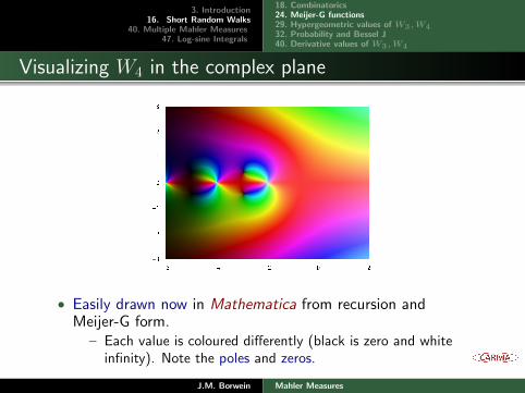
Visualizing W4 in the complex plane
• Easily drawn now in Mathematica from recursion andMeijer-G form.
– Each value is coloured differently (black is zero and whiteinfinity). Note the poles and zeros.
J.M. Borwein Mahler Measures

3. Introduction16. Short Random Walks
40. Multiple Mahler Measures47. Log-sine Integrals
18. Combinatorics24. Meijer-G functions29. Hypergeometric values of W3,W432. Probability and Bessel J40. Derivative values of W3,W4
Visualizing W4 in the complex plane
• Easily drawn now in Mathematica from recursion andMeijer-G form.
– Each value is coloured differently (black is zero and whiteinfinity). Note the poles and zeros.
J.M. Borwein Mahler Measures

3. Introduction16. Short Random Walks
40. Multiple Mahler Measures47. Log-sine Integrals
18. Combinatorics24. Meijer-G functions29. Hypergeometric values of W3,W432. Probability and Bessel J40. Derivative values of W3,W4
Simplifying the Meijer integral
Corollary (Hypergeometric forms for noninteger s > −2)
W3(s) =1
22s+1tan
(πs
2
)(ss−12
)2
3F2
(12, 12, 12
s+32, s+3
2
∣∣∣∣ 14
)+
(s
s2
)3F2
(− s
2,− s
2,− s
2
1,− s−12
∣∣∣∣ 14
),
and
W4(s) =1
22stan
(πs
2
)(ss−12
)3
4F3
(12, 12, 12, s2
+ 1
s+32, s+3
2, s+3
2
∣∣∣∣1)
+
(s
s2
)4F3
(12,− s
2,− s
2,− s
2
1, 1,− s−12
∣∣∣∣1).
• We (humans) were able to provably take the limit:
W4(−1) =π
47F6
(54, 12, 12, 12, 12, 12, 12
14, 1, 1, 1, 1, 1
∣∣∣∣1)
=π
4
∞∑n=0
(4n + 1)(2nn
)646n
=π
46F5
(12, 12, 12, 12, 12, 12
1, 1, 1, 1, 1
∣∣∣∣1)
+π
646F5
(32, 32, 32, 32, 32, 32
2, 2, 2, 2, 2
∣∣∣∣1).
• We have proven the corresponding result for W4(1) ....
J.M. Borwein Mahler Measures

3. Introduction16. Short Random Walks
40. Multiple Mahler Measures47. Log-sine Integrals
18. Combinatorics24. Meijer-G functions29. Hypergeometric values of W3,W432. Probability and Bessel J40. Derivative values of W3,W4
Hypergeometric values of W3,W4: from Meijer-G values.
With much work involving moments of elliptic integrals we finallyobtain:
Theorem (Tractable hypergeometric form for W3)
(a) For s 6= −3,−5,−7, . . . , we have
W3(s) =3s+3/2
2πβ
(s+
1
2, s+
1
2
)3F2
(s+2
2 , s+22 , s+2
2
1, s+32
∣∣∣∣14).
(6)
(b) For every natural number k = 1, 2, . . .,
W3(−2k − 1) =
√3(
2kk
)224k+132k 3F2
( 12 ,
12 ,
12
k + 1, k + 1
∣∣∣∣14).
J.M. Borwein Mahler Measures

3. Introduction16. Short Random Walks
40. Multiple Mahler Measures47. Log-sine Integrals
18. Combinatorics24. Meijer-G functions29. Hypergeometric values of W3,W432. Probability and Bessel J40. Derivative values of W3,W4
A Discovery Demystified: on piecing all this togetherWe first proved that:
W3(2k) =∑
a1+a2+a3=k
(k
a1, a2, a3
)2
= 3F2
(1/2,−k,−k
1, 1
∣∣∣∣4)︸ ︷︷ ︸=:V3(2k)
.
We discovered numerically that: V3(1) = 1.57459− .12602652i
Theorem (Real part)
For all integers k we have W3(k) = Re (V3(k)).
We have a habit in writing articles published in scientific journals to
make the work as finished as possible, to cover up all the tracks, to not
worry about the blind alleys or describe how you had the wrong idea first.
. . . So there isn’t any place to publish, in a dignified manner, what you
actually did in order to get to do the work. — Richard Feynman (Nobel
acceptance 1966)
J.M. Borwein Mahler Measures

3. Introduction16. Short Random Walks
40. Multiple Mahler Measures47. Log-sine Integrals
18. Combinatorics24. Meijer-G functions29. Hypergeometric values of W3,W432. Probability and Bessel J40. Derivative values of W3,W4
Closed Forms for W3
• We then confirmed 175 digits of
W3(1) ≈ 1.57459723755189365749 . . .
• Armed with a knowledge of elliptic integrals:
W3(1) =16 3√
4π2
Γ(13)6
+3Γ(1
3)6
8 3√
4π4= W3(−1) +
6/π2
W3(−1),
W3(−1) =3Γ(1
3)6
8 3√
4π4=
213
4π2β2
(1
3
).
Here β(s) := B(s, s) = Γ(s)2
Γ(2s) .
• Obtained via singular values of the elliptic integral andLegendre’s identity.
J.M. Borwein Mahler Measures

3. Introduction16. Short Random Walks
40. Multiple Mahler Measures47. Log-sine Integrals
18. Combinatorics24. Meijer-G functions29. Hypergeometric values of W3,W432. Probability and Bessel J40. Derivative values of W3,W4
Probability: Bessel function representations
1906. J.C. Kluyver (1860-1932) derived the cumulative radialdistribution function (Pn) and density (pn) of the n-step distance:
Pn(t) = t
∫ ∞0
J1(xt) Jn0 (x) dx
pn(t) = t
∫ ∞0
J0(xt) Jn0 (x)x dx (n ≥ 4) (7)
where Jn(x) is a Bessel function of the first kind• See also Watson (1932, §49) – 3-dim walks are elementary.
• From (9) below, we find
pn(1) = Res−2 (Wn+1) (n 6= 4). (8)
• As p2(α) = 2π√
4−α2, we check in Maple that the following
code returns R = 2/(√
3π) symbolically:R:=identify(evalf[20](int(BesselJ(0,x)^3*x,x=0..infinity)))
J.M. Borwein Mahler Measures

3. Introduction16. Short Random Walks
40. Multiple Mahler Measures47. Log-sine Integrals
18. Combinatorics24. Meijer-G functions29. Hypergeometric values of W3,W432. Probability and Bessel J40. Derivative values of W3,W4
A Bessel Integral for Wn
• Now Pn(1) = J0(0)n+1
n+1 = 1n+1 (Pearson’s original question).
• Broadhurst used (7) for 2k > s > −n2 to write
Wn(s) = 2s+1−k Γ(1 + s2)
Γ(k − s2)
∫ ∞0
x2k−s−1
(−1
x
d
dx
)kJn0 (x)dx,
(9)a useful oscillatory 1-dim integral (used below).
• Thence
Wn(−1) =
∫ ∞0
Jn0 (x)dx, Wn(1) = n
∫ ∞0
J1(x)J0(x)n−1 dx
x.
(10)
Integrands for W4(−1) (blue) andW4(1) (red) on [π, 4π] from (10).
J.M. Borwein Mahler Measures

3. Introduction16. Short Random Walks
40. Multiple Mahler Measures47. Log-sine Integrals
18. Combinatorics24. Meijer-G functions29. Hypergeometric values of W3,W432. Probability and Bessel J40. Derivative values of W3,W4
The Densities for n = 3, 4 are ModularLet σ(x) := 3−x
1+x . Then σ is an involution on [0, 3] sending [0, 1] to [1, 3]:
p3(x) =4x
(3− x)(x+ 1)p3(σ(x)).
So 34p′3(0) = p3(3) =
√3
2π , p(1) =∞. We found:
p3(α) =2√3α
π(3 + α2
) 2F1
13, 23
1
∣∣∣∣α2(9− α2
)2(3 + α2
)3 =
2√3
π
α
AG3(3 + α2, 3(1− α2
)2/3)where AG3 is the cubically convergent mean iteration (1991):
AG3(a, b) :=a + 2b
3
⊗(b ·
a2 + ab + b2
3
)1/3
. The densities p3 (L) and p4 (R)
J.M. Borwein Mahler Measures

3. Introduction16. Short Random Walks
40. Multiple Mahler Measures47. Log-sine Integrals
18. Combinatorics24. Meijer-G functions29. Hypergeometric values of W3,W432. Probability and Bessel J40. Derivative values of W3,W4
Formula for the ‘shark-fin’ p4
We ultimately deduce on 2 ≤ α ≤ 4 a hyper-closed form:
p4(α) =2
π2
√16− α2
α3F2
(12 ,
12 ,
12
56 ,
76
∣∣∣∣(16− α2
)3108α4
). (11)
← p4 from (11) vs 18-terms of series
X Proves p4(2) = 27/3π3√3
Γ(23
)−6=
√3π W3(−1) ≈ 0.494233 < 1
2
• Marvelously, we found — and provedby a subtle use of distributional Mellintransforms — that on [0, 2] as well:
p4(α) =2
π2
√16− α2
αRe 3F2
(12 ,
12 ,
12
56 ,
76
∣∣∣∣(16− α2
)3108α4
)(Discovering this Re brought us full circle.)
J.M. Borwein Mahler Measures

3. Introduction16. Short Random Walks
40. Multiple Mahler Measures47. Log-sine Integrals
18. Combinatorics24. Meijer-G functions29. Hypergeometric values of W3,W432. Probability and Bessel J40. Derivative values of W3,W4
Densities for 5 ≤ n ≤ 8 (and large n approximation)
1 2 3 4 5
0.05
0.10
0.15
0.20
0.25
0.30
0.35
1 2 3 4 5 6
0.05
0.10
0.15
0.20
0.25
0.30
0.35
Both p2n+4, p2n+5 are n-times continuously differentiable for x > 0
(pn(x) ∼ 2xn e−x2/n). So “four is small” but “eight is large.”
1 2 3 4 5 6 7
0.05
0.10
0.15
0.20
0.25
0.30
2 4 6 8
0.05
0.10
0.15
0.20
0.25
0.30
J.M. Borwein Mahler Measures

3. Introduction16. Short Random Walks
40. Multiple Mahler Measures47. Log-sine Integrals
18. Combinatorics24. Meijer-G functions29. Hypergeometric values of W3,W432. Probability and Bessel J40. Derivative values of W3,W4
The Five Step Walk
• The functional equation for W5 is:
225(s + 4)2(s + 2)
2W5(s) = −(35(s + 5)
4+ 42(s + 5)
2+ 3)W5(s + 4)
+ (s + 6)4W5(s + 6) + (s + 4)
2(259(s + 4)
2+ 104)W5(s + 2).
• We deduce the first two poles — and so all — are simple since
lims→−2
(s+ 2)2W5(s) =4
225(285W5(0)− 201W5(2) + 16W5(4)) = 0
lims→−4
(s+ 4)2W5(s) = − 4
225(5W5(0)−W5(2)) = 0.
• We stumbled upon
p4(1) =Res−2(W5) =
√15
3π3F2
( 13 ,
23 ,
12
1, 1
∣∣∣∣−4
).
??? Is there a hyper-closed form for W5(∓1) ???J.M. Borwein Mahler Measures

3. Introduction16. Short Random Walks
40. Multiple Mahler Measures47. Log-sine Integrals
18. Combinatorics24. Meijer-G functions29. Hypergeometric values of W3,W432. Probability and Bessel J40. Derivative values of W3,W4
W5 and p5: Bessel integrals are hard
• We only know Res−4(W5) numerically — but to 500 digits:• by Bailey in about 5.5hrs on 1 MacPro core.
– Sidi-“mW” method used: i.e., Gaussian quadrature onintervals of [nπ, (n+ 1)π] plus Richardson-like extrapolation.
– Can r5(2) be identified?
• Here r5(k) := Res(−2k)(W5). Other residues are thencombinations as follows:
• From the W5-recursion: given r5(0) = 0, r5(1) and r5(2) we have
r5(k + 3) =k4r5(k)−
(5 + 28 k + 63 k2 + 70 k3 + 35 k4
)r5(k + 1)
225(k + 1)2(k + 2)2
+
(285 + 518 k + 259 k2
)r5(k + 2)
225(k + 2)2.
J.M. Borwein Mahler Measures

3. Introduction16. Short Random Walks
40. Multiple Mahler Measures47. Log-sine Integrals
18. Combinatorics24. Meijer-G functions29. Hypergeometric values of W3,W432. Probability and Bessel J40. Derivative values of W3,W4
W5 and p5: Bessel integrals are hard
• We only know Res−4(W5) numerically — but to 500 digits:• by Bailey in about 5.5hrs on 1 MacPro core.
– Sidi-“mW” method used: i.e., Gaussian quadrature onintervals of [nπ, (n+ 1)π] plus Richardson-like extrapolation.
– Can r5(2) be identified?
• Here r5(k) := Res(−2k)(W5). Other residues are thencombinations as follows:
• From the W5-recursion: given r5(0) = 0, r5(1) and r5(2) we have
r5(k + 3) =k4r5(k)−
(5 + 28 k + 63 k2 + 70 k3 + 35 k4
)r5(k + 1)
225(k + 1)2(k + 2)2
+
(285 + 518 k + 259 k2
)r5(k + 2)
225(k + 2)2.
J.M. Borwein Mahler Measures
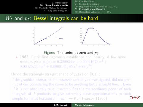
3. Introduction16. Short Random Walks
40. Multiple Mahler Measures47. Log-sine Integrals
18. Combinatorics24. Meijer-G functions29. Hypergeometric values of W3,W432. Probability and Bessel J40. Derivative values of W3,W4
W5 and p5: Bessel integrals can be hard
0.5 1.0 1.5 2.0 2.5
0.2
0.4
0.6
0.8
1 2 3 4 5
0.05
0.10
0.15
0.20
0.25
0.30
0.35
Figure: The series at zero and p5.• 1963. Fettis first rigorously established nonlinearity. A few more
residues yield p5(x) = 0.329934x+ 0.00661673x3 +0.000262333x5 + 0.0000141185x7 +O(x9)
Hence the strikingly straight shape of p5(x) on [0, 1] :
“the graphical construction, however carefully reinvestigated, did not per-mit of our considering the curve to be anything but a straight line. . . Evenif it is not absolutely true, it exemplifies the extraordinary power of suchintegrals of J products to give extremely close approximations to suchsimple forms as horizontal lines.” — Karl Pearson (1906)
J.M. Borwein Mahler Measures

3. Introduction16. Short Random Walks
40. Multiple Mahler Measures47. Log-sine Integrals
18. Combinatorics24. Meijer-G functions29. Hypergeometric values of W3,W432. Probability and Bessel J40. Derivative values of W3,W4
Short Random Walks: Derivatives of W3,W4
From the hypergeometric forms above we get:
W ′3(0) =1
π3F2
(12 ,
12 ,
12
32 ,
32
∣∣∣∣14)
=1
πCl(π
3
). (12)
The last equality follows from setting θ = π/6 in the identity
2 sin(θ)3F2
(12 ,
12 ,
12
32 ,
32
∣∣∣∣sin2 θ
)= Cl (2 θ) + 2 θ log (2 sin θ) .
Also
W ′4(0) =4
π2 4F3
(12 ,
12 ,
12 , 1
32 ,
32 ,
32
∣∣∣∣1)
=7ζ(3)
2π2. (13)
Here Cl(θ) :=∑∞
n=1sin(nθ)
n2 is Clausen’s function. Likewise:
W′3(2) =
3
πCl(π
3
)− 3√
3
2π+ 2 . . .
J.M. Borwein Mahler Measures

3. Introduction16. Short Random Walks
40. Multiple Mahler Measures47. Log-sine Integrals
42. Relations to η43. Smyth’s results revisited45. Boyd’s Conjectures47. A Bonus Measure
Multiple Mahler Measures: for P1, P2, . . . , Pm toc
µ(P1, P2, . . . , Pm) :=
∫ 1
0
· · ·∫ 1
0
m∏k=1
log∣∣Pk (e2πiθ1 , · · · , e2πiθn)∣∣ dθ1 · · · dθn,
was introduced by Sasaki (2010); while
µm(P ) := µ(P,P, . . . , P ), (µ1(P ) = µ(P ))
is a higher Mahler measure as in Kurakowa, Lalın and Ochiai(2008). Also
µm
(1 +
n−1∑k=1
xk
)= W (m)
n (0), (14)
was evaluated in (12), (13) for n = 3 and n = 4 and m = 1:
1 µ(1 + x+ y) = L′3(−1) = 1
π Cl(π3
)(Smyth)
2 µ(1 + x+ y + z) = 14 ζ′(−2) = 7
2ζ(3)π2 (Smyth)
– So (14) recaptured both Smyth’s results.
J.M. Borwein Mahler Measures

3. Introduction16. Short Random Walks
40. Multiple Mahler Measures47. Log-sine Integrals
42. Relations to η43. Smyth’s results revisited45. Boyd’s Conjectures47. A Bonus Measure
Relations to Dedekind’s η
Denninger’s 1997 conjecture, proven recently by Rogers andZudilin (2011), is
µ(1 + x+ y + 1/x+ 1/y)?=
15
4π2LE(2)
– an L-series value for an elliptic curve E with conductor 15.
• For (14) with n = 5, 6 conjectures of Villegas become:
W′
5(0)?=
(15
4π2
)5/2 ∫ ∞0
{η3(e−3t)η3(e−5t) + η3(e−t)η3(e−15t)
}t3 dt
W′
6(0)?=
(3
π2
)3 ∫ ∞0
η2(e−t)η2(e−2t)η2(e−3t)η2(e−6t) t4 dt
where Dedekind’s η is η(q) := q1/24∑∞
n=−∞(−1)nqn(3n+1)/4.
• Confirmed to 600 and to 80 digits respectively.
J.M. Borwein Mahler Measures

3. Introduction16. Short Random Walks
40. Multiple Mahler Measures47. Log-sine Integrals
42. Relations to η43. Smyth’s results revisited45. Boyd’s Conjectures47. A Bonus Measure
µ(1 + x+ y) and µ(1 + x+ y + z) revisited
We recall:
Lemma (Jensen’s formula)∫ 1
0log∣∣α+ e2πi t
∣∣ dt = log (max{|α|, 1}) . (15)
We use (15) to reduce to a one dimensional integral:
µ(1 + x+ y) =
∫ 5/6
1/6log(2 sin(πy)) dy =
1
πLs2
(π3
)=
1
πCl2
(π3
),
which is (12).
J.M. Borwein Mahler Measures

3. Introduction16. Short Random Walks
40. Multiple Mahler Measures47. Log-sine Integrals
42. Relations to η43. Smyth’s results revisited45. Boyd’s Conjectures47. A Bonus Measure
µ(1 + x+ y) and µ(1 + x+ y + z) revisited
Following Boyd, on applying Jensen’s formula, for complex a and bwe have µ(ax+ b) = log |a| ∨ log |b|. Let w := y/z. We now write
µ(1 + x+ y + z) = µ(1 + x+ z(1 + w)) = µ(log |1 + w| ∨ log |1 + x|)
=1
π2
∫ π
0
dθ
∫ π
0
max
{log
(2 sin
θ
2
), log 2
(sin
t
2
)}dt
=2
π2
∫ π
0
dθ
∫ θ
0
log
(2 sin
θ
2
)dt
=2
π2
∫ π
0
θ log
(2 sin
θ
2
)dθ
= − 2
π2Ls
(1)3 (π) =
7
2
ζ(3)
π2,
which is (13).
J.M. Borwein Mahler Measures

3. Introduction16. Short Random Walks
40. Multiple Mahler Measures47. Log-sine Integrals
42. Relations to η43. Smyth’s results revisited45. Boyd’s Conjectures47. A Bonus Measure
Boyd’s 1998 Conjectures
Theorem (Two quadratic evaluations)
Below L−n is a primitive L-series and G is Catalan’s constant.
µ3 := µ(y2(x+ 1)2 + y(x2 + 6x+ 1) + (x+ 1)2) =16
3πL−4(2)
=16
3πG,
µ−5 := µ(y2(x+ 1)2 + y(x2 − 10x+ 1) + (x+ 1)2) =5√
3
πL−3(2)
=20
3πCl2
(π3
).
J.M. Borwein Mahler Measures

3. Introduction16. Short Random Walks
40. Multiple Mahler Measures47. Log-sine Integrals
42. Relations to η43. Smyth’s results revisited45. Boyd’s Conjectures47. A Bonus Measure
Log-sine Integrals are Again Inside
First proven in 2008 using Bloch-Wigner logarithms, we used avariant of Jensen’s formula and slick trigonometry to arrive at:
µ3 =1
π
∫ π
0log(1 + 4| cos θ|+ 4| cos2 θ|) dθ
=4
π
∫ π/2
0log(1 + 2 cos θ) dθ
=4
π
∫ π/2
0log
(2 sin 3θ
2
2 sin θ2
)dθ
=4
3π
(Ls2
(3π
2
)− 3 Ls2
(π2
))=
16
3
L−4(2)
π
as needed, since Ls2
(3π2
)= −Ls2
(π2
)= L−4(2), which is
Catalan’s G.J.M. Borwein Mahler Measures

3. Introduction16. Short Random Walks
40. Multiple Mahler Measures47. Log-sine Integrals
42. Relations to η43. Smyth’s results revisited45. Boyd’s Conjectures47. A Bonus Measure
And More
Much the same techniques work for µ5 and there is one bonus case:
Theorem
π µ−1 = π µ((x+ 1)2(y2 + y + 1)− 2xy
)=
1
2B
(1
4,
1
4
)3F2
(14 ,
14 , 1
34 ,
54
∣∣∣∣14)− 1
6B
(3
4,
3
4
)3F2
(34 ,
34 , 1
54 ,
74
∣∣∣∣14)
An alternative form of µ−1 is given by
µ−1 = µ((x+ 1/x+ 2
√1/x)
(y + 1/y + 1)− 2).
J.M. Borwein Mahler Measures

3. Introduction16. Short Random Walks
40. Multiple Mahler Measures47. Log-sine Integrals
42. Relations to η43. Smyth’s results revisited45. Boyd’s Conjectures47. A Bonus Measure
And More
Much the same techniques work for µ5 and there is one bonus case:
Theorem
π µ−1 = π µ((x+ 1)2(y2 + y + 1)− 2xy
)=
1
2B
(1
4,
1
4
)3F2
(14 ,
14 , 1
34 ,
54
∣∣∣∣14)− 1
6B
(3
4,
3
4
)3F2
(34 ,
34 , 1
54 ,
74
∣∣∣∣14)
An alternative form of µ−1 is given by
µ−1 = µ((x+ 1/x+ 2
√1/x)
(y + 1/y + 1)− 2).
J.M. Borwein Mahler Measures

3. Introduction16. Short Random Walks
40. Multiple Mahler Measures47. Log-sine Integrals
48. Sasaki’s Mahler Measures51. Log-sine-cosine integrals56. Three Cognate Evaluations58. KLO’s Mahler Measures62. Conclusion
Sasaki’s Multiple Mahler Measures toc
µk(1 + x+ y∗) := µ(1 + x+ y1, 1 + x+ y2, . . . , 1 + x+ yk)
was studied by Sasaki (2010). He used (15) to observe that
µk(1 + x+ y∗) = −∫ 5/6
1/6logk
∣∣1 + e2πi t∣∣ dt (16)
and so provides an evaluation of µ2(1 + x+ y∗). Immediately from(16) and the definition of the log-sine integrals we have:
Theorem (For k = 1, 2, ...)
µk(1 + x+ y∗) =1
π
{Lsk+1
(π3
)− Lsk+1 (π)
}, (17)
where Lsk+1 is as given by (1).
J.M. Borwein Mahler Measures

3. Introduction16. Short Random Walks
40. Multiple Mahler Measures47. Log-sine Integrals
48. Sasaki’s Mahler Measures51. Log-sine-cosine integrals56. Three Cognate Evaluations58. KLO’s Mahler Measures62. Conclusion
Lsk (π) and Ls(k)n (π)
− 1
π
∞∑m=0
Lsm+1 (π)um
m!=
Γ (1 + u)
Γ2(1 + u
2
) =
(u
u/2
). (18)
Example (Values of Lsn (π))
For instance, we have Ls2 (π) = 0 as well as
−Ls3 (π) =1
12π3 Ls4 (π) =
3
2π ζ(3)
−Ls5 (π) =19
240π5 Ls6 (π) =
45
2π ζ(5) +
5
4π3ζ(3)
−Ls7 (π) =275
1344π7 +
45
2π ζ2(3)
J.M. Borwein Mahler Measures

3. Introduction16. Short Random Walks
40. Multiple Mahler Measures47. Log-sine Integrals
48. Sasaki’s Mahler Measures51. Log-sine-cosine integrals56. Three Cognate Evaluations58. KLO’s Mahler Measures62. Conclusion
Lsn (π) and Ls(k)n (π)
Equation (18) is made for a CAS (Mma, Sage or Maple):for k to 7 do
simplify(subs(x=0,diff(Pi*binomial(x,x/2),x$k))) od
We studied general log-sine evaluations with an emphasis onautomatic provable evaluations. For example:
Theorem (Borwein-Straub)
For 2|µ| < λ < 1 we have
−∑n,k≥0
Ls(k)n+k+1 (π)
λn
n!
(iµ)k
k!= i∑n≥0
(λ
n
)(−1)neiπ
λ2 − eiπµ
µ− λ2 + n
.
J.M. Borwein Mahler Measures
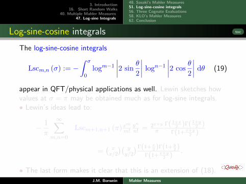
3. Introduction16. Short Random Walks
40. Multiple Mahler Measures47. Log-sine Integrals
48. Sasaki’s Mahler Measures51. Log-sine-cosine integrals56. Three Cognate Evaluations58. KLO’s Mahler Measures62. Conclusion
Log-sine-cosine integrals toc
The log-sine-cosine integrals
Lscm,n (σ) := −∫ σ
0logm−1
∣∣∣∣2 sinθ
2
∣∣∣∣ logn−1
∣∣∣∣2 cosθ
2
∣∣∣∣ dθ (19)
appear in QFT/physical applications as well. Lewin sketches howvalues at σ = π may be obtained much as for log-sine integrals.• Lewin’s ideas lead to:
− 1
π
∞∑m,n=0
Lscm+1,n+1 (π)xm
m!yn
n! = 2x+y
π
Γ( 1+x2 )Γ( 1+y
2 )Γ(1+x+y
2 )
=(xx/2
)( yy/2
)Γ(1+x2 )Γ(1+ y
2 )Γ(1+x+y
2 ).
• The last form makes it clear that this is an extension of (18).J.M. Borwein Mahler Measures

3. Introduction16. Short Random Walks
40. Multiple Mahler Measures47. Log-sine Integrals
48. Sasaki’s Mahler Measures51. Log-sine-cosine integrals56. Three Cognate Evaluations58. KLO’s Mahler Measures62. Conclusion
Ls(k)n (τ) is Made of Sterner Stuff.
• Contour integration and “polylogarithmics” yield:
Theorem (Reduction Theorem for 0 ≤ τ ≤ 2π )
For n, k such that n− k ≥ 2, we have
ζ(k, {1}n)−k−2∑j=0
(−iτ)j
j!Lik−j,{1}n (e
iτ)
=(−i)k−1
(k − 2)!
(−1)n
(n + 1)!
n+1∑r=0
r∑m=0
(n + 1
r
)(r
m
)(i
2
)r(−π)r−mLs
(k+m−2)n+k−(r−m)
(τ).
where Li2+k−j,{1}n−k−2(eiτ ) is a harmonic polylogarithm and
ζ(n− k, {1}k) is an Euler-Zagier sum.
J.M. Borwein Mahler Measures

3. Introduction16. Short Random Walks
40. Multiple Mahler Measures47. Log-sine Integrals
48. Sasaki’s Mahler Measures51. Log-sine-cosine integrals56. Three Cognate Evaluations58. KLO’s Mahler Measures62. Conclusion
Ls(k)n
(π3
): A small miracle occurs: e−i
π3 = ei
π3 .
The Reduction Theorem now lets us find all values of Ls(k)n
(π3
)and so of µk(1 + x+ y∗):
Example (Values of Lsn (π/3))
Ls2
(π3
)= Cl2
(π3
)− Ls3
(π3
)=
7
108π3
Ls4
(π3
)=
1
2π ζ(3) +
9
2Cl4
(π3
)−Ls5
(π3
)=
1543
19440π5 − 6 Gl4,1
(π3
)Ls6
(π3
)=
15
2π ζ(5) +
35
36π3ζ(3) +
135
2Cl6
(π3
)−Ls7
(π3
)=
74369
326592π7 +
15
2πζ(3)2 − 135 Gl6,1
(π3
)J.M. Borwein Mahler Measures
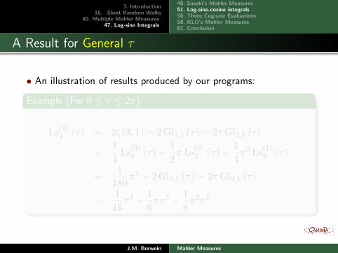
3. Introduction16. Short Random Walks
40. Multiple Mahler Measures47. Log-sine Integrals
48. Sasaki’s Mahler Measures51. Log-sine-cosine integrals56. Three Cognate Evaluations58. KLO’s Mahler Measures62. Conclusion
A Result for General τ
• An illustration of results produced by our programs:
Example (For 0 ≤ τ ≤ 2π)
Ls(1)4 (τ) = 2ζ(3, 1)− 2 Gl3,1 (τ)− 2τ Gl2,1 (τ)
+1
4Ls
(3)4 (τ)− 1
2π Ls
(2)3 (τ) +
1
4π2 Ls
(1)2 (τ)
=1
180π4 − 2 Gl3,1 (τ)− 2τ Gl2,1 (τ)
− 1
16τ4 +
1
6πτ3 − 1
8π2τ2.
J.M. Borwein Mahler Measures
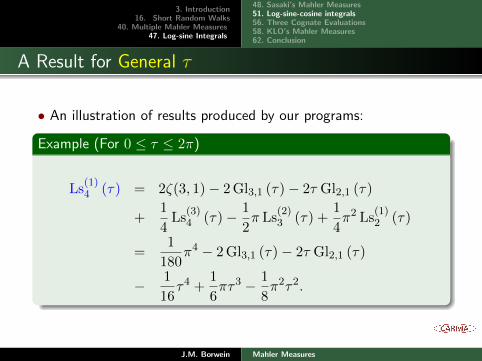
3. Introduction16. Short Random Walks
40. Multiple Mahler Measures47. Log-sine Integrals
48. Sasaki’s Mahler Measures51. Log-sine-cosine integrals56. Three Cognate Evaluations58. KLO’s Mahler Measures62. Conclusion
Irreducibility and Binomial Sums
Example (The first presumably irreducible value for π/3)
Gl4,1
(π3
)=
∞∑n=1
∑n−1k=1
1k
n4sin(nπ
3
)=
3341
1632960π5 − 1
πζ2(3)− 3
4π
∞∑n=1
1(2nn
)n6
while always
Ls(1)n+2
(π3
)=
n!(−1)n+1
2n
∞∑k=1
1
kn+2(
2kk
) .• Alternating binomial sums come from imaginary values of τ
via log sinh integrals at ρ = 1+√
52 .
J.M. Borwein Mahler Measures

3. Introduction16. Short Random Walks
40. Multiple Mahler Measures47. Log-sine Integrals
48. Sasaki’s Mahler Measures51. Log-sine-cosine integrals56. Three Cognate Evaluations58. KLO’s Mahler Measures62. Conclusion
First EvaluationLet
µk(1 + x+ y∗ + z∗) := µ(1 + x+ y1 + z1, . . . , 1 + x+ yk + zk).(20)
Theorem
For all positive integers k, we have
µk(1 + x+ y∗ + z∗) = − 1
πk+1
∫ π
0
(θ log
(2 sin
θ
2
)− Cl2 (θ)
)kdθ
Then
µ1(1 + x+ y∗ + z∗) = − 2
π2Ls
(1)3 (π) =
7
2
ζ(3)
π2,
µ2(1 + x+ y∗ + z∗) = − 1
π3Ls
(2)5 (π) +
π2
90=
4
π2Li3,1(−1) +
7
360π2.
J.M. Borwein Mahler Measures

3. Introduction16. Short Random Walks
40. Multiple Mahler Measures47. Log-sine Integrals
48. Sasaki’s Mahler Measures51. Log-sine-cosine integrals56. Three Cognate Evaluations58. KLO’s Mahler Measures62. Conclusion
Two More Evaluations: with Kummer-type logarithmsLet
λn(x) := (n− 2)!
n−2∑k=0
(−1)k
k!Lin−k(x) logk |x|+ (−1)n
nlogn |x|,
so that
λ1
(12
)= log 2, λ2
(12
)=
1
2ζ(2), λ3
(12
)=
7
8ζ(3),
and λ4
(12
)is the first to reveal the presence of Lin
(12
). From the
value of W′′4 (0) we derive:
Theorem
µ2(1 + x+ y + z) =12
π2λ4
(12
)− π2
5
µ(1 + x, 1 + x, 1 + x+ y + z) =4
3π2λ5
(12
)− 3
4ζ(3) +
31
16π2ζ(5).
J.M. Borwein Mahler Measures

3. Introduction16. Short Random Walks
40. Multiple Mahler Measures47. Log-sine Integrals
48. Sasaki’s Mahler Measures51. Log-sine-cosine integrals56. Three Cognate Evaluations58. KLO’s Mahler Measures62. Conclusion
KLO’s Mahler Measures
Theorem (Hypergeometric forms for µn(1 + x+ y))
For complex |s| < 2, we may write
∞∑n=0
µn(1 + x+ y)sn
n!=
√3
2π3s+1 Γ(1 + s
2 )2
Γ(s+ 2)3F2
(s+22 , s+2
2 , s+22
1, s+32
∣∣∣∣14)(21)
=
√3
π
(3
2
)s+1 ∫ 1
0
z1+s2F1
(1+ s
2 ,1+s2
1
∣∣∣∣ z24 )√
1− z2dz.
J.M. Borwein Mahler Measures

3. Introduction16. Short Random Walks
40. Multiple Mahler Measures47. Log-sine Integrals
48. Sasaki’s Mahler Measures51. Log-sine-cosine integrals56. Three Cognate Evaluations58. KLO’s Mahler Measures62. Conclusion
Evaluation of µn(1 + x+ y) Requires a Taylor Expansion
Consider
3F2
(ε+2
2 , ε+22 , ε+2
2
1, ε+32
∣∣∣∣14)
=
∞∑n=0
αnεn. (22)
Indeed, from (21) and Leibniz’ rule we have
µn(1 + x+ y) =
√3
2π
n∑k=0
(n
k
)αkβn−k (23)
where βk is defined by
3ε+1 Γ(1 + ε2)2
Γ(ε+ 2)=
∞∑n=0
βnεn.
Note, as above, that βk is easy to compute.J.M. Borwein Mahler Measures

3. Introduction16. Short Random Walks
40. Multiple Mahler Measures47. Log-sine Integrals
48. Sasaki’s Mahler Measures51. Log-sine-cosine integrals56. Three Cognate Evaluations58. KLO’s Mahler Measures62. Conclusion
Faa di Bruno’s Formula
We can now read off the terms αn of the ε-expansion:
Theorem (For n = 0, 1, 2, . . .)
Let Ak,j :=∑2j−1m=2
2(−1)m+1−1mk
. Then
[εn] 3F2
(ε+22 , ε+2
2 , ε+22
1, ε+32
∣∣∣∣14)
= (−1)n∞∑j=1
2
j
1(2jj
) ∑ n∏k=1
Amkk,jmk!kmk
(24)
where we sum over all m1, . . . ,mn with m1 + 2m2 + . . .+ nmn = n.
Proof.
Equation (24) follows from (21) on using Faa di Bruno’s formula for then-th derivative of the composition on two functions via Pochhammernotation.
J.M. Borwein Mahler Measures

3. Introduction16. Short Random Walks
40. Multiple Mahler Measures47. Log-sine Integrals
48. Sasaki’s Mahler Measures51. Log-sine-cosine integrals56. Three Cognate Evaluations58. KLO’s Mahler Measures62. Conclusion
Davydychev and Kalmykov’s Binomial Sums Yield:
Example
µ1(1 + x+ y) =3
2πLs2
(2π
3
)µ2(1 + x+ y) =
3
πLs3
(2π
3
)+π2
4
µ3(1 + x+ y)?=
6
πLs4
(2π
3
)− 9
πCl4
(π3
)− π
4Cl2
(π3
)− 1
2ζ(3).
As we had obtained by other methods. Also PSLQ then finds:
πµ4(1 + x+ y)?= 12 Ls5
(2π
3
)− 49
3Ls5
(π3
)+ 81 Gl4,1
(2π
3
)+ 3π2 Gl2,1
(2π
3
)+ 2ζ(3) Cl2
(π3
)+ πCl2
(π3
)2− 29
90π5.
J.M. Borwein Mahler Measures
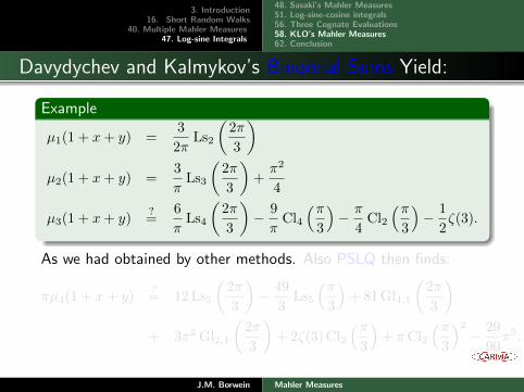
3. Introduction16. Short Random Walks
40. Multiple Mahler Measures47. Log-sine Integrals
48. Sasaki’s Mahler Measures51. Log-sine-cosine integrals56. Three Cognate Evaluations58. KLO’s Mahler Measures62. Conclusion
Davydychev and Kalmykov’s Binomial Sums Yield:
Example
µ1(1 + x+ y) =3
2πLs2
(2π
3
)µ2(1 + x+ y) =
3
πLs3
(2π
3
)+π2
4
µ3(1 + x+ y)?=
6
πLs4
(2π
3
)− 9
πCl4
(π3
)− π
4Cl2
(π3
)− 1
2ζ(3).
As we had obtained by other methods. Also PSLQ then finds:
πµ4(1 + x+ y)?= 12 Ls5
(2π
3
)− 49
3Ls5
(π3
)+ 81 Gl4,1
(2π
3
)+ 3π2 Gl2,1
(2π
3
)+ 2ζ(3) Cl2
(π3
)+ πCl2
(π3
)2− 29
90π5.
J.M. Borwein Mahler Measures

3. Introduction16. Short Random Walks
40. Multiple Mahler Measures47. Log-sine Integrals
48. Sasaki’s Mahler Measures51. Log-sine-cosine integrals56. Three Cognate Evaluations58. KLO’s Mahler Measures62. Conclusion
Conclusion
We also have generalized arctangent forms, such as:
µ2(1 +x+ y) =24
5πTi3
(1√3
)+
2 log 3
πCl2
(π3
)− log2 3
10− 19π2
180.
1 We are still hunting for a complete accounting ofµn(1 + x+ y).
2 Our log-sine and MZV algorithms uncovered many errors inthe literature.
3 Automated simplification, validation and correction tools aremore and more important.
4 Congratulations to all!
J.M. Borwein Mahler Measures