Macroscopic modeling of multi-lane motorways using a two-dimensional second-order model of traffic flow

Michael Herty*, Salissou Moutari‡ and Giuseppe Visconti*

Institut für Geometrie und Praktische Mathematik Templergraben 55, 52062 Aachen, Germany

* InstitutfurGeometrieundPraktischeMathematik(IGPM),RWTH-AachenUniversity,Templergraben55, 52062Aachen,Germany‡SchoolofMathematicsandPhysics,MathematicalSciencesResearchCentre,Queens‘University,Belfast,BT71NN, NorthernIreland,UnitedKingdom

O C

T O

B E

R

2 0

1 7

P

R E

P R

I N T

4

7 1

Macroscopic modeling of multi-lane motorways using a

two-dimensional second-order model of traffic flow

Michael HertyInstitut fur Geometrie und Praktische Mathematik (IGPM)

RWTH Aachen University

Templergraben 55, 52062 Aachen, Germany

Salissou MoutariSchool of Mathematics and Physics

Mathematical Sciences Research Centre

Queens’ University, Belfast

BT7 1NN, Northern Ireland, United Kingdom

Giuseppe ViscontiInstitut fur Geometrie und Praktische Mathematik (IGPM)

RWTH Aachen University

Templergraben 55, 52062 Aachen, Germany

October 11, 2017

Abstract

Lane changing is one of the most common maneuvers on motorways. Although, macro-scopic traffic models are well known for their suitability to describe fast moving crowdedtraffic, most of these models are generally developed in one dimensional framework, hence-forth lane changing behavior is somehow neglected. In this paper, we propose a macroscopicmodel, which accounts for lane-changing behavior on motorway, based on a two-dimensionalextension of the Aw and Rascle [4] and Zhang [19] macroscopic model for traffic flow. Underconditions, when lane changing maneuvers are no longer possible, the model “relaxes” to theone-dimensional Aw-Rascle-Zhang model. Following the same approach as in [3], we derivethe two-dimensional macroscopic model through scaling of time discretization of a microscopicfollow-the-leader model with driving direction. We provide a detailed analysis of the space-time discretization of the proposed macroscopic as well as an approximation of the solutionto the associated Riemann problem. Furthermore, we illustrate some features of the proposedmodel through some numerical experiments.

MSC 90B20; 35L65; 35Q91; 91B74

Keywords Traffic flow, macroscopic model, two dimensional model, second-order traffic flowmodels

1 Introduction

Current macroscopic models for multi-lane traffic on motorways generally couple a multi-lane ormulti-class one-dimensional first-order model of traffic flow (LWR model) [15, 17] with some lane-changing rules in order to capture traffic dynamics stemming from the lane-changing maneuvers [6,

1

9, 11, 12, 16]. A major assumption of the LWR model is that for a given traffic density allthe drivers adopt the same velocity. However, this assumption is not always valid in practice.Macroscopic second-order models, e.g. [4, 19], attempted to address this limitation by introducingan additional variable, which in [8] was interpreted as an “relative” velocity of a specific (class)of drivers. The advection of the “relative” velocity with the actual velocity enable to describethe reaction of drivers to traffic conditions ahead of them. Therefore, second-order models can beviewed as an extension of the LWR such that, for a given traffic density, drivers can react differently,by adopting a wide range of speed. In [3] the derivation of the second-order macroscopic Aw-Rascle-Zhang model [4, 19] was proposed. More recently, in [7], the “follow-the-leader” approximationof the Aw-Rascle-Zhang model was proposed in a multi population framework with also a deepdiscussion on the analytical properties of the model.

In a recent preprint, Herty and Visconti [10] used microscopic data, namely vehicle trajectoriescollected on a German highway, to derive a two-dimensional first-order macroscopic model. Thecurrent study used the same experimental microscopic data to derive a macroscopic model formulti-lane traffic on highways based on a two-dimensional extension of the Aw-Rascle-Zhangmodel [4, 19]. By revisiting the analysis proposed in [3], we show that the semi-discretization ofthe two-dimensional Aw-Rascle-Zhang model can be viewed as the limit of a multi-lane “follow-the-leader” model. These results enable the two-dimensional macroscopic model to capture trafficdynamics due to the lane-changing behavior in spite coarse scale traffic flow description. Numericalsimulations give an evidence of the link between the two models belonging to different scales aswell as the ability of both models to reproduce classical traffic situations. We stress the fact thathere we use a classical first order finite volume scheme since we are only aimed in showing thelink between the microscopic and the macroscopic description of traffic flow. However, suitablenumerical strategies should be used to approximate the macroscopic equations and, for instance,we refer to [5] where a scheme being able to remove the oscillations near to contact discontinuitieswas proposed.

We highlight that in [1, 2] a derivation of a two-dimensional macroscopic crowd model isderived from a microscopic one. Furthermore, in this work, we provide a detailed analysis of theapproximation of the solution to the associated Riemann problem. The main idea behind theapproximation of the solution to the two-dimensional Riemann problem was the coupling of two-half Riemann problems in one dimension and then use the transition from one lane to another,subject to some admissibility conditions, in order to capture the two-dimensional aspect of theproblem. We provide a detailed discussion, of the main scenarios under consideration in this study,as well as the suitable Riemann solvers at the interfaces of the lanes which describe the lateraldynamics caused by lane-changing maneuvers. An enjoyable feature of the proposed model is itsdouble-sided behavior. Under conditions, when lane-changing maneuvers are no longer possible,e.g. the traffic is congested on adjacent lanes, the model “relaxes” to the one-dimensional Aw-Rascle-Zhang model [4, 19], whereas in free flow conditions on adjacent lanes, the model capturesdynamics caused by car movement between adjacent lanes.

The remaining part of the paper is organized as follows. Section 2 presents a brief overview ofthe one-dimensional Aw-Rascle-Zhang [4, 19] model reviewing some of its mathematical propertiesrelevant to the current study. In particular, we will revisit it using a different approach fro itsderivation from the microscopic “follow-the-leader” model. Section 3 and Section 4 introduce theproposed 2D macroscopic model and outline and discuss sufficient conditions for the derivationof the model through some scaling of the time discretization of a microscopic “follow-the-leader”model with driving direction. A detailed analysis of the two-dimensional macroscopic model as wellas an approximation of the solution to the associated Riemann problem have also been providedin Section 5. In Section 6, we discuss the space-time discretization of the proposed macroscopicand we show some numerical simulations illustrating some interesting features of the proposedmodel, are presented and discussed. Finally, Section 7 concludes the paper and highlighted somedirections for further research.

2

2 Preliminary discussions

We start by reviewing the paper [3] in which the authors show a connection between the classicalmicroscopic “follow-the-leader” (FTL) model and the Aw and Rascle [4] and Zhang [19] (ARZ)macroscopic model. More precisely, they prove that the FTL model can be viewed as semi-discretization of the ARZ model in Lagrangian coordinates. However, here we prove the connectionbetween the two models using a different approach in the case of two-dimensional models.

Contrary to [3] we consider a two-dimensional FTL model first and derive the correspondingmacroscopic limiting equations using suitable coordinate transformations. In order to illustratethe idea we briefly recall the homogeneous and conservative form of the second-order traffic flowmodel [4, 19].

∂tρ(t, x) + ∂x(ρu)(t, x) = 0,

∂t(ρw)(t, x) + ∂x(ρuw)(t, x) = 0,(1)

where w(t, x) = u(t, x) + P and P = P (ρ) is the so called “traffic pressure”.The corresponding one–dimensional microscopic model is based on the following arguments.

The movement of particles is described according to xi = ui, where xi = xi(t) and ui = ui(t) arethe time-dependent position and speed, respectively, of vehicle i. If not specified, the quantitiesare assumed at time t. In Lagrangian coordinate the particles move along with the trajectory.The local density at time t is defined as

ρi =∆X

xj(i) − xi(2)

where ∆X is the typical length of a vehicle and τi = 1/ρi describes the relative distance evolving.The index j(i) identifies the interacting vehicle for a car i. Let us assume, without loss in generality,that cars are ordered as xi < xi+1, ∀ i. Then, under this hypothesis, we have j(i) = i+1. Therefore,the distance between i and i+ 1 car evolves as

τi(t+ ∆t)− τi(t) =xi+1(t+ ∆t)− xi+1(t)− (xi(t+ ∆t)− xi(t))

∆X.

Dividing by ∆t and taking the limit leads to

τi =ui+1 − ui

∆X. (3)

We define a macroscopic velocity by ui(t) =: uL(t,Xi) where Xi = X(t, xi) is the cumulative carmass up to car label i at time t. By definition

X(t, x) =

∫ x

ρ(t, ξ)dξ. (4)

Notice that we are assuming that time is not influenced by the transformation from the discretedynamics. In a discrete model with N cars we define the density around car i as ρ(t, x) =

1∆X

∑Nk=1 δ(x−xk(t)). The total mass is then N/∆X (instead of δ distributions one could suitable

regularize). Therefore, we obtain X(t, xi) = 1∆X

(∑i−1l=1 1 + 1

2

). Since the cars are ordered as xi <

xi+1, then, for each fixed time t, the map s 7→ X(t, s) for the given density is a monotone function.Therefore, there is a one-to-one map from i to X(t, xi). Hence, we denote by Xi = X(t, xi). Then,we can extend the values ui to a function uL such that, at each time t, ui(t) = uL(t,Xi). Weproceed similarly for τi.

Finally, from equation (3) we obtain

∂tτL(t,Xi) =

uL(t,Xi+1)− uL(t,Xi)

∆X

that is a finite volume semi-discretization of the PDE

∂tτL − ∂XuL = 0, (5)

provided the following assumptions:

3

Ansatz 1 we have one car per cell and the distance between two cell centers is precisely ∆X, i.e.∆X is the grid space.

Ansatz 2 τL and uL are distributed as piecewise constant on each cell[Xi− 1

2, Xi+ 1

2

].

Notice that the first assumption means that we are considering the macroscopic limit in whichthe number of vehicles goes to infinity whereas the length of cars shrinks to zero. The secondassumption implies we are considering a first-order finite–volume scheme and does not pose aserious restriction.

Now, let us to consider the equation for the acceleration in the “follow-the-leader” modelwithout relaxation

ui = Uref∆Xγ vi+1 − vi

(xi+1 − xi)γ+1.

Let wi = ui + P (τi) where P (τi) is a function defined as

P (τi) =

Uref

γτγi, γ > 0

−Uref ln(τi), γ = 0.

Then, straightforward computations show that wi = ui + P ′(τi)τi = 0, which can represent thesecond equation of the particle model. Again, we can identify wi(t) = wL(t,Xi) and thus we get

∂twL = 0. (6)

As proved in [3], equation (5) and equation (6) give the Lagrangian version of the ARZmodel (1). Thus, we have showed that from the microscopic FTL model is derived as a semi-discretization of the macroscopic ARZ model in Lagrangian coordinates.

In Figure 1 we provide the same simulation proposed in [3] in order to give a numerical evidenceof the link between the two models. The blue dotted line is the initial condition for the density ρand the flux ρu, while the red solid line and the orange circles give the solution of the macroscopicand of the microscopic model, respectively. We refer to [3] for further details on the simulationparameters.

3 Derivation of a spatially two-dimensional extension of theARZ model

In this section we will derive the extension of the ARZ model to the case of two space dimensions.To this end, we will introduce a generalization of the FTL model with dynamics including lanechanging and then we will use the similar arguments to Section 2 to derive the macroscopic model.

In a two-dimensional microscopic model we have to consider the evolution in time of thepositions along and also across the road section. Let xi = xi(t) and yi = yi(t) be the time-dependent positions, then they evolve according to

xi = ui, yi = vi,

for all vehicles i = 1, . . . , N . The speed ui is supposed to be non-negative (travel in x-direction),while vi can be either positive or negative (travel in y-direction).

In contrast to the one-dimensional case, we assume that there is no particular ordering imposedright now, we simply label the cars. The occupied space by each car is ∆X∆Y , where ∆X and ∆Yare the typical length and the typical width, respectively, of a vehicle. Generalizing the definitionof the one-dimensional case, the density around vehicle i becomes

ρi =∆X∆Y(

xj(i) − xi) ∣∣yj(i) − yi∣∣ (7)

4

-100 -50 0 50 100

-0.02

0

0.02

0.04

0.06

FTL vs ARZ model

-100 -50 0 50 100

-0.02

0

0.02

0.04

Initial condition ARZ FTL

Figure 1: Simulation of the 1D ARZ model (red solid line) and of the 1D FTL model (orangecircles). The top panel shows the density, while the bottom panel shows the flux at initial time(dotted line) and at final time.

y

x

xj(i) − xi

yj(i)−

yii

j(i)

∆Y

∆X

∆Y

∆X

y

x

xj(i) − xi

yi−

yj(i)

i

j(i)

∆Y

∆X

∆Y

∆X

Figure 2: Different position between the test vehicle i and the interacting vehicle j(i). Left: they-distance is yj(i) − yi > 0. Right: the y-distance is yi − yj(i) > 0.

where the interacting vehicle is labeled by j(i). Since here we do not assume any order on thelabeling, in general j(i) 6= i + 1. The absolute value in (7) is considered in order to take intoaccount both the situations displayed in Figure 2, depending on the relative position of vehiclej(i) with respect to vehicle i, and thus to guarantee the positivity of the density. Using thecoordinate system in Figure 2 we assume that a vehicle i moves towards the left side of the roadif vi > 0 and towards the right side if vi < 0.

Remark 1. Let ρ1Di and ρ2Di be the local density in the one-dimensional (see (2)) and in the

5

θ1

θ2θ3

θ = 0

θ = π/2

θ /∈ [−π/2, π/2]

θ /∈ [−π/2, π/2]

vi sin (θ1) < 0

vi sin(θk

)> 0, k = 2, 3

y

x

i

2

3

1

Figure 3: Choice of the interacting car in the case vi > 0. The interacting vehicle will be car 2,namely the nearest vehicle in the driving direction of vehicle i.

two-dimensional case (see (7)), respectively. Observe that

ρ2Di → ρ1Di , as ∆Y,∣∣yj(i) − yi∣∣→ 0+

only if we assume that

lim∆Y→0+

(yj(i)−yi)→0+

∆Y∣∣yj(i) − yi∣∣ = 1. (8)

The interacting vehicle j(i) is determined by the following map

i 7→ j(i) = arg minh=1,...,Nvi sin θh>0

θh∈[−π2 ,π2 ]

‖Qh −Qi‖2 . (9)

This choice is motivated as follows, see also Figure 3. Assume that each test vehicle i defines acoordinate system in which the origin is its right rear corner if vi ≥ 0 and its left rear corner ifvi < 0. We are indeed dividing the road in four areas. Let θh be the angle between the x-axis (inthe car coordinate system) and the position vector Qh of vehicle h. Then the request θh ∈

[−π2 ,

π2

]allows to consider only cars being in front of vehicle i. Instead, the request vi sin θh > 0 allowsto consider only cars in the driving direction of vehicle i. Among all these vehicles we choose thenearest one. Therefore, (9) can be rewritten as

i 7→ j(i) = arg minh=1,...,N

vi(yh−yi)>0xh>xi

‖Qh −Qi‖2 .

6

The specific volume for car i is defined as τi := 1/ρi and thus we have

τi =

(xj(i) − xi

) ∣∣yj(i) − yi∣∣∆X∆Y

.

From elementary geometry we obtain as in the one-dimensional case

τi(t+ ∆t)− τi(t) =

(xj(i) − xi

) ∣∣yj(i) − yi∣∣ (t+ ∆t)

∆X∆Y−(xj(i) − xi

) ∣∣yj(i) − yi∣∣ (t)∆X∆Y

.

Now, we add and subtract(xj(i)−xi)(t)|yj(i)−yi|(t+∆t)

∆X∆Y , and send ∆t to zero to obtain the finaldynamics

τi =

(uj(i) − ui

) ∣∣yj(i) − yi∣∣∆X∆Y

+

(vj(i) − vi

) ∣∣yj(i) − yi∣∣ (xj(i) − xi)∆Y∆X

(yj(i) − yi

) . (10)

As in the one-dimensional case, we wish to identify τi with a function out of the discretedynamics in order to find the corresponding conservation law. Then, we introduce

X =

∫ x

ρ(t, ξ, η)dξ, Y =

∫ y

ρ(t, ξ, η)dη

for some values η, ξ. They are the cumulative car mass up to car label i in x-direction (andprojected on y = η) and in y-direction (and projected on x = ξ), respectively.

Again, we would like to relate the label of the car to a corresponding mass. The discretemeasure corresponding to N cars is now

ρ(t, x, y) =1

∆X∆Y

N∑i=1

δ(x− xi(t))δ(y − yi(t))

with total mass N/∆X/∆Y.In order to obtain the one-to-one relation between the label i and the pair of indices (k, `)

corresponding to the cumulative masses Xk and Y`, we proceed as follows. We view the cars aspoints in the 2D domain. Now, we fix an arbitrary value η in y-direction and project all carstowards this line, i.e., from (xi, yi) to (xi, η). Then, the projected density is given by

ρ(t, x, η) =1

∆X∆Y

N∑i=1

δ(x− xi(t)).

Then, computing X on the projected density gives

X(t, xi, η) =1

∆X∆Y

∑h|xh∈(−∞,xi]

1 +1

2

=1

∆X∆Y

(k +

1

2

)

for some k.Similarly, we fix ξ in x direction and project all cars towards this line, i.e., from (xi, yi) to

(ξ, yi). We obtain

Y (t, ξ, yi) =1

∆X∆Y

∑h|xh∈(−∞,yi]

1 +1

2

=1

∆X∆Y

(`+

1

2

)

for some `.Note that k and ` may well be different according to the position of the vehicles. Moreover,

for each fixed time t, the definition does not depend on the choice of η and ξ.

7

Again, in the projected densities, the maps s 7→ X(t, s, y) and s 7→ Y (t, x, s) are monotonefunctions. Hence, for those quantities at least for short time there is a one-to-one correspondencebetween car i and the pair (k, `), respectively. Therefore, we can identify

τi = τL(t,Xk, Y`)

and similarly for the speeds

ui = uL(t,Xk, Y`), vi = vL(t,Xk, Y`).

Since we are interested in the limit for many cars it is natural to assume that there are enoughcars in the neighboring cells. We therefore assume:

Ansatz j(i) 7→ (k + 1, `+ 1) if vi ≥ 0 and j(i) 7→ (k + 1, `− 1) if vi < 0.

Now, observe that, since X and Y are monotone we can write

xi = X−1

(1

∆X∆Y

(k +

1

2

)), yi = Y −1

(1

∆X∆Y

(`+

1

2

)).

Assume that vi is positive, then we obtain that

yj(i) − yi = Y −1

(1

∆X∆Y

(`+ 1 +

1

2

))− Y −1

(1

∆X∆Y

(`+

1

2

))= ∆Y

by straightforward computation using the fact that the map Y is locally invertible.Similar computations hold for the case vi < 0 and in the x-direction. Therefore, equation (10)

writes as

τi =

(uj(i) − ui

)∆X

+

(vj(i) − vi

) ∣∣yj(i) − yi∣∣∆Y

(yj(i) − yi

) . (11)

Now, we show that (11) can be seen as a suitable semi-discretization in space of (12).

∂tτL − ∂XuL − ∂Y vL = 0. (12)

We consider a uniform cartesian grid

Ωk,` =[Xk− 1

2, Xk+ 1

2

]×[Y`− 1

2, Y`+ 1

2

]in which Xk+ 1

2= Xk + ∆X and Y`+ 1

2= Y` + ∆X and we define the volume average

τLk,`(t) =1

∆X∆Y

∫∫Ωk,`

τL(t, ξ, η)dξdη.

Integrating the conservation law over each control volume and dividing by the volume of Ωk,` weobtain the finite volume formulation of (12)

d

dtτLk,` =

1

∆X∆Y

∫ Y`+1

2

Y`− 1

2

(uL(t,Xk+ 1

2, η)− uL(t,Xk− 1

2, η))dη

+1

∆X∆Y

∫ Xk+1

2

Xk− 1

2

(vL(t, ξ, Y`+ 1

2)− vL(t, ξ, Y`− 1

2))dξ.

(13)

We consider a first-order finite–volume scheme. This implies that τL, uL and vL are given aspiecewise constant on each of the above patches. In this interpretation the mass of the car isuniformly distributed on the path ∆X ×∆Y and thus, for the specific volume we have

τLk,`(t) = τL(t,Xk, Y`).

8

Since the velocity along the road is non-negative, then for the first term in the right-hand sideof (13) an Upwind flux would be appropriate and in this case uL(t,Xk+ 1

2, η) ≈ uL(t,Xk+1, η).

Then, we write1

∆X∆Y

∫ Y`+1

2

Y`− 1

2

(uL(t,Xk+1, η)− uL(t,Xk, η)

)dη.

Since uL is constant on the patch, we evaluate it at any point η ∈[Y`− 1

2, Y`+ 1

2

]. We choose to

evaluate now at different points in Y direction, so that we finally get for the first term in theright-hand side of (13)

1

∆X

(uL(t,Xk+1, Y`+1)− uL(t,Xk, Y`)

)For the second term in the right-hand side of (13) we notice that the speed across the lanes

can be either positive or negative. We again use an Upwind flux. However, if the velocity ispositive then the approximation vL(t, ξ, Y`+ 1

2) ≈ vL(t, η, Y`+1) is still appropriate. In contrast, if

the velocity is negative we take vL(t, ξ, Y`+ 12) ≈ vL(t, η, Y`). Thus, we obtain

1

∆X∆Y

∫ Xk+1

2

Xk− 1

2

(vL(t, ξ, Y`+1)− vL(t, ξ, Y`)

)dξ, if vL(t,Xk, Y`) ≥ 0

1

∆X∆Y

∫ Xk+1

2

Xk− 1

2

(vL(t, ξ, Y`)− vL(t, ξ, Y`−1)

)dξ, if vL(t,Xk, Y`) < 0.

Since also vL is constant on the patch, we can evaluate it at any point ξ ∈[Xk− 1

2, Xk+ 1

2

]. We

choose to evaluate at different points in X direction, so that we can finally obtain1

∆Y

(vL(t,Xk+1, Y`+1)− vL(t,Xk, Y`)

), if vL(t,Xk, Y`) ≥ 0

1

∆Y

(vL(t,Xk, Y`)− vL(t,Xk−1, Y`−1)

), if vL(t,Xk, Y`) < 0.

Putting together all the terms, from (13) we have

d

dtτLk,` =

1

∆X

(uLk+1,`+1(t)− uLk,`(t)

)+

v+

∆Y

(vLk+1,`+1(t)− vLk,`(t)

)+

v−

∆Y

(vLk,`(t)− vLk−1,`−1(t)

)where v+ = max

(0,|vLk,`(t)|vLk,`(t)

)and v− = min

(0,|vLk,`(t)|vLk,`(t)

). Thus, we (11) is a first-order finite

volume semi-discretization of the conservation law (12).Now, we study what happens for the acceleration. Actually, since a two-dimensional FTL

model has not already been introduced in literature, we do not have the evolution equation forthe acceleration in the two-dimensional case at hand. Thus, we first need to derive the equationsfor ui and vi.

We define two quantities

wi = ui + P1(τi), σi = vi + P2(τi),

which can be seen as desired speeds of vehicle i in the x- and in the y-direction, respectively. Thequantities P1 and P2 play the role of the “traffic pressure” and they are functions of the localdensity. However, observe that P1 and P2 should be homogeneous to a velocity a for this reasonwe take P1 6= P2 assuming that there are two different reference velocities in the two differentdirections of the flow. We define

P1(τi) =

Uref

γ1τγ1i

, if γ1 > 0

−Uref ln(τi), if γ1 > 0

, P2(τi) =

Vref

γ2τγ2i

, if γ2 > 0

−Vref ln(τi), if γ2 > 0

(14)

9

and as in the one-dimensional model without relaxation we require that the desired speeds areconstant during the time evolution, that is

wi = σi = 0.

We therefore obtainui = −τiP ′1(τi), vi = −τiP ′2(τi)

and computing the derivative of P1 and P2 with respect to τi we can finally get the equation forthe evolution of the microscopic accelerations

ui = C1

(uj(i) − ui(

xj(i) − xi)

∆Aγ1+

vj(i) − vi(yj(i) − yi

)∆Aγ1

)

vi = C2

(uj(i) − ui(

xj(i) − xi)

∆Aγ2+

vj(i) − vi(yj(i) − yi

)∆Aγ2

)

where

C1 = Uref∆Xγ1∆Y γ1 , C2 = Vref∆X

γ2∆Y γ2 , ∆A =(xj(i) − xi

) ∣∣yj(i) − yi∣∣ .Remark 2. Notice that the above equations for the microscopic accelerations are consistent to

ui = Uref∆Xγ1

uj(i) − ui(xj(i) − xi

)γ1+1

vi = 0

which are the acceleration equations in the one-dimensional case in the limit Vref → 0 and underhypothesis (8).

Remark 3. In the macroscopic limit, i.e. when the number of cars increases whereas xj(i)−xi =

∆X and∣∣yj(i) − yi∣∣ = ∆Y , we simply get

ui = Uref

(uj(i) − ui(xj(i) − xi

) +vj(i) − vi(yj(i) − yi

))

vi = Vref

(uj(i) − ui(xj(i) − xi

) +vj(i) − vi(yj(i) − yi

))

Finally, the two-dimensional “follow-the-leader” microscopic model is

xi = ui,

yi = vi,

ui = C1

(uj(i) − ui(

xj(i) − xi)

∆Aγ1+

vj(i) − vi(yj(i) − yi

)∆Aγ1

),

vi = C2

(uj(i) − ui(

xj(i) − xi)

∆Aγ2+

vj(i) − vi(yj(i) − yi

)∆Aγ2

) (15)

which can be, altogether, rewritten in the form

τi =

(uj(i) − ui

)∆X

+

(vj(i) − vi

) ∣∣yj(i) − yi∣∣∆Y

(yj(i) − yi

) ,

wi = 0,

σi = 0.

(16)

10

0 20 40 60 80 100 1200

1

2

3

4

5

6

7

8

9Real vs computed trajetories

Car 1Car 2Car 3Car 4Car 5Car 6Car 7Real Trajectory

520 520.5 521 521.5 5220

2

4

6

8

10

122-norm error of the trajectories

Car 1Car 2Car 3Car 4Car 5Car 6Car 7

Figure 4: Left: comparison between the real trajectories provided by experimental data in [10] andthe computed trajectories using the two-dimensional microscopic model (15). Right: evolution ofthe 2-norm error in time for each car.

We have already seen that the equation for the time evolution of the specific volume (thefirst in (16)) is first-order finite volume semi-discretization of the conservation law in Lagrangiancoordinates (12). Since there exists a one-to-one map i 7→ (k, `) we may extend the values wi andσi to two functions wL(t,X, Y ) and σL(t,X, Y ) such that

wi(t) = wL(t,Xk, Y`), σi(t) = σL(t,Xk, Y`)

where wL and σL are defined as

wL(t,X, Y ) = uL(t,X, Y ) + P1

(τL(t,X, Y )

), σL(t,X, Y ) = vL(t,X, Y ) + P2

(τL(t,X, Y )

).

Assuming a first-order scheme and thus assuming that wL and σL are constant on the grid, wi = 0and σi = 0 can be obviously viewed as semi-discretization of

∂twL = 0, ∂tσ

L = 0.

Finally, the above equation and (12) define the system of macroscopic equations in Lagrangiancoordinates writes as

∂tτL = ∂Xu

L + ∂Y vL, ∂tw

L = 0, , ∂tσL = 0. (17)

Remark 4 (Validation of the 2D particle model). In [10] we used the experimental data providedfrom a German highway in order to derive a two-dimensional first-order macroscopic model. Themicroscopic trajectories of vehicles were used to compute macroscopic quantities related to trafficflow and consequently fundamental diagrams. These latter were used to define a closure for themacroscopic equation. Here, we use the same microscopic data introduced in [10] to validate thetwo-dimensional microscopic model (15). To this end, we fix an initial time and using experimentaldata we get the initial positions and speeds of vehicles on the road. We compute the interactingvehicle for each car using (9) and then we evolve the trajectories using (15). The right-mostvehicle in x-direction is used as ghost car and its trajectory is updated at each time using thereal trajectory. In the left panel of Figure 4 we show the real trajectories (red line) provided byexperimental data and the computed trajectories with the 2D microscopic model (black symbols),after 2 seconds. In the right panel of Figure 4 we show the error between the real and the computedtrajectory for each car, using the 2-norm distance.

4 From Lagrangian to Eulerian coordinates

Macroscopic equations (17) are written with respect to the “mass” coordinates (or Lagrangian) Xand Y where the variables X(t, x, y) and Y (t, x, y) denote the total mass of vehicles up to point x

11

and up to point y, for y = y and x = x fixed, respectively.We reformulate the model in Eulerian coordinates x and y by setting t(T,X, Y ) = T and

x(t,X, Y ) =

∫ X

τL(t, ξ, Y )dξ, y(t, X, Y ) =

∫ Y

τL(t, X, η)dη.

From this definition and using the continuity equation in Lagrangian coordinates we obtain

∂Xx = ∂Y y = τL, ∂tx = uL, ∂ty = vL, ∂Y x = ∂Xy = 0.

The Jacobian of the coordinate transformation is given by

J =∂(T,X, Y )

∂(t, x, y)=

1 0 0

uL τL 0

vL 0 τL

.and therefore the continuity equation in Lagrangian coordinates (12) yields the correspondingequation in Eulerian variables

∂τ

∂t+ u

∂τ

∂x+ v

∂τ

∂y= τ

∂u

∂x+ τ

∂v

∂y.

Recalling that τ = 1/ρ we get∂ρ

∂t+∂(ρu)

∂x+∂(ρv)

∂y= 0. (18)

For the momentum equation, we discuss the case ∂twL = 0 with the other equation being

similar. From∂tu

L + P ′1(ρL)∂tρL = 0.

we compute

ρ∂u

∂t+ ρu

∂u

∂x+ ρv

∂u

∂y− ρ2P ′1(ρ)

∂u

∂x− ρ2P ′1(ρ)

∂v

∂y= 0.

and therefore we finally obtain in conservative form

∂ρw

∂t+∂ρuw

∂x+∂ρvw

∂y= 0. (19)

Finally, the system of macroscopic equations in Eulerian coordinates writes as

∂tρ+ ∂x(ρu) + ∂y(ρv) = 0,

∂t(ρw) + ∂x(ρuw) + ∂y(ρvw) = 0,

∂t(ρσ) + ∂x(ρuσ) + ∂y(ρvσ) = 0.

(20)

We end the section with the following remarks on the 2D ARZ-type model (20).

Remark 5. If v = Vref = 0 we recover the one-dimensional ARZ model (1).If we substitute the continuity equation in the two equations for the speeds we get

∂tw + u∂xw + v∂yw = 0

∂tσ + u∂xσ + v∂yσ = 0

which are transport equations for w and σ.Recall that w = u + P1(ρ) and σ = v + P2(ρ). Let w = c1 and σ = c2 be constants. Then the

system of three equations reduces to

∂tρ+ ∂x (ρ(c1 − P1(ρ))) + ∂y (ρ(c2 − P2(ρ))) .

12

Assuming γ1 = 1 and taking c1 = Uref we obtain the Greenshields’ law for the x direction

u = Uref(1− ρ).

Changing the values of c1 or γ1 will let to obtain several diagrams, as already studied in [18].For the y direction instead we have

v = c2 − P2(ρ) = c2 −Vrefγ2

ργ2 ,

where Vref < 0 is the reference velocity in y and it is negative as compared by data. Also in thiscase if c2 = Vref and γ2 = 1 we get a linear function such that v = Vref for ρ = 0 and v = 0 forρ = 1. Actually, as done in our previous paper, the parameters c2 and γ2 can be chosen to fit thedata and they allow to obtain different diagrams, shifted from the naive one if we modify c2, orwith a different shape if we modify γ2.

5 Properties of the two-dimensional ARZ model

For simplicity of the following discussion we consider the following non-conservative form of the2D Aw-Rascle model:

∂tρ+ ∂x(ρu) + ∂y(ρv) = 0, (21)

(∂t + u∂x + v∂y)(u+ P1(ρ) = 0, (22)

(∂t + u∂x + v∂y)(v + P2(ρ)) = 0. (23)

Using the continuity equation (21) in equations (22)-(23), the system is written in in matrixnotations with U = (ρ, u, v)T

∂tU +A(U)∂xU +B(U)∂yU = 0, (24)

where

A(U) =

u ρ 00 u− ρP ′1(ρ) 00 v −ρP ′1(ρ)

and B(U) =

v 0 ρ0 −ρP ′2(ρ) u0 0 v − ρP ′2(ρ)

A system of the form (24) is said to be hyperbolic if for any ξ = (ξ1, ξ2) ∈ R2 the matrix

C(U, ξ) = ξ1A+ ξ2B is diagonalizable [13]. This is the case here and the eigenvalues of the matrixC(U, ξ) are

λ1 = −(ξ1ρP′1(ρ) + ξ2ρP

′2(ρ)) ≤ λ2 = ξ1(u− ρP ′1(ρ)) + ξ2(v − ρP ′2(ρ)) ≤ λ3 = ξ1u+ ξ2v.

The eigenvalues of C(U, ξ) for |ξ| = 1 correspond to the wave speeds and the their correspondingeigenvectors are respectively

r1 =

−(u+v)v(P ′1(ρ)+P ′2(ρ))

u/v1

, r2 =

0−11

, and r3 =

100

.

Remark 6. Observe that, as in the classical Aw-Rascle-Zhang model [4, 19], the system is nothyperbolic in presence of a vacuum state, i.e. if ρ = 0.

The second and third eigenvalues, λ2 and λ3, are linearly degenerate since∇λ2·r1 = ∇λ3·r2 = 0(here ∇ := (∂ρ, ∂u, ∂v)). For the first eigenvalue, we have

∇λ1 · r1 =[P ′1(ρ) + P ′2(ρ) + ρ(P ′′1 (ρ) + P ′′2 (ρ))](u+ v)

v(P ′1(ρ) + P ′2(ρ)).

13

Clearly, there exist (ρ, u, v) ∈ R∗+ × R∗+ × R∗+ such that ∇λ1 · r1 6= 0. Therefore λ1 is notlinearly degenerate. For the other fields to be genuinely nonlinear we need to show ∇λ1 · r1 6= 0for all (ρ, u, v) 6= (0, 0, 0). This condition is fulfilled provided that the functions P1(ρ) and P2(ρ)fulfill

∂ρ(ρP′1(ρ)) 6= ∂ρ(ρP

′2(ρ)).

The above condition is satisfied as long as the reference velocities Uref and Vref , introduced in(14), are different. Since λ1 is genuinely nonlinear, for Uref 6= Vref , then the associated waves areeither shocks or rarefaction waves.

The Riemann invariants, in the sense of Lax [14], associated with the eigenvalues λ1, λ2 andλ3 are respectively:

z1 = u+ v + P1(ρ) + P2(ρ), z2 = u+ v, z3 = u.

5.1 An overview of the Riemann problem associated to the system

The main idea behind the approximation of the solution to the two-dimensional Riemann problemwas the coupling of two-half Riemann problems in one dimension and then use the transition fromone lane to another, subject to some admissibility conditions. In this section, we provide a detaileddiscussion, of the main scenarios under consideration in this study, as well as the suitable Riemannsolvers at the interfaces of the lanes in order to capture the two-dimensional aspect of the problem.Following this approach, the solution to the system (21)-(23) consists of either a wave of the firstfamily (1-shock or 1-rarefaction) or a wave of the second family (2-contact discontinuity). Theproperties of these two families of waves can be summarized as follows.

First characteristic field: A wave of the first family is generated when a state on left, denotedUl = (ρl, ul, vl), is connect to a state on the right, denotes Ur = (ρr, ur, vr), through the sameRiemann invariant curve associated with the eigenvalue λ1, i.e. z1(Ul) = z1(Ur). Therefore, wehave

ul + vl + P1(ρl) + P2(ρl) = ur + vr + P1(ρr) + P2(ρr). (25)

We can distinguish the following scenarios:

• if ul + vl > ur + vr, then this wave (of the first family) is a 1-shock i.e. a jump discontinuity,traveling with the speed

s =ρr(ur + vr)− ρl(ul + vl)

ρr − ρl. (26)

• if ul + vl < ur + vr, then this wave (of the first family) is a 1-rarefaction, i.e. a continuous

solution of the form (ρ, u, v)(ξ) (with ξ = f(x,y)t ), given byρ′(ξ)u′(ξ)

v′(ξ)

=r1(U(ξ))

∇λ1(U(ξ)) · r1(U(ξ)), if λ1(Ul) ≤ ξ ≤ λ1(Ur), (27)

whereas

(ρ, u, v)(ξ) =

(ρl, ul, vl) for ξ < λ1(Ul),

(ρr, ur, vr) for ξ > λ1(Ur).

Second characteristic field: A wave of the second family i.e. a 2-contact discontinuity isgenerated when

z2(Ul) = z2(Ur) =⇒ ul + vl = ur + vr.

In this case, the contact discontinuity between a state on the left, Ul = (ρl, ul, vl), and a state onthe right, Ur = (ρr, ur, vr), travels with a speed η = ul + vl = ur + vr.

14

Third characteristic field: A wave of the third family i.e. a 3-contact discontinuity is generatedwhen

z3(Ul) = z3(Ur) =⇒ ul = ur.

In this case, the contact discontinuity between a state on the left, Ul = (ρl, ul, vl), and a state onthe right, Ur = (ρr, ur, vr), travels with a speed η = ul = ur.

5.2 Solution to the Riemann problem associated with the system (21)-(23)

This section describes the solutions to the Riemann problem for the system (21)-(23), by combiningthe previously described elementary. Let Ul = (ρl, ul, vl) and Ur = (ρr, ur, vr) be the initial dataon the left and on the right, respectively. The solutions to the system (21)-(23) for these initialdata consist of the following cases.

Case 1. If σl = vl + P2(ρl) = σr = vr + P2(ρr) = 0, then the model bowls down to the one-dimensional Aw-Rascle model i.e. the initial data reduced to Ul = (ρl, ul) and Ur = (ρr, ur).Therefore, the state on the left Ul = (ρl, ul) is connect to an intermediate state U? = (ρ?, u?)through a wave of the first family, i.e. either a 1-shock wave if ul > ur (which corresponds tobraking) or a 1-rarefaction wave if ul < ur (which corresponds to an acceleration). Then, theintermediate state U? is connected to the state on the right Ur = (ρr, ur) through a wave ofthe second family, i.e. a 2-contact discontinuity. Therefore, an admissible intermediate state,U? = (ρ?, u?), is defined such that:

u? = ur and ρ? = P−11 (ul + u? + P1(ρl)).

Case 2. If σl = vl + P2(ρl) = σr = vr + P2(ρr) > 0, then we have the following admissiblescenarios:

• If vl = σl − P2(ρl) > 0 (lane changing possibility), then the state on the left Ul = (ρl, ul, vl)is connected to an intermediate state on the left, U?l = (ρ?l , u

?l , v

?l ), through a wave of the

first family, i.e. either a 1-shock (if ul > ur) or a rarefaction wave (if ul < ur). Then, theintermediate state U?l is connected to a vacuum state through a wave of the second family,i.e. a 2-contact discontinuity. Therefore, an admissible intermediate state, U?l = (ρ?l , u

?l , v

?l ),

is defined such that: ul + P1(ρl) = u?l + P1(ρ?l ),

vl + P2(ρl) = v?l + P2(ρ?l ),

u?l = ul + vl.

The vacuum state, is then connected to an intermediate state on the right, U?r = (ρ?r , u?r , v

?r ),

through a wave of the first family, i.e. either a 1-shock (if u?l > u?r) or a 1-rarefactionwave (if u?l < u?r). Then, the intermediate state, U?r , is connected to the state on theright, Ur = (ρr, ur, vr), through a wave of the third family, i.e. a 3-contact discontinuity.Therefore, an admissible intermediate state, U?r = (ρ?r , u

?r , v

?r ), is defined such that:

u?l + P1(ρ?l ) = u?r + P1(ρ?r),

v?l + P2(ρ?l ) = v?r + P2(ρ?r),

u?r = ur.

• If vl = σl−P2(ρl) = 0 (no lane changing possibility), then the state on the left Ul = (ρl, ul, vl)is connected to an intermediate state on the left, U?l = (ρ?l , u

?l , v

?l ), through a 1-rarefaction

wave. Then, the intermediate state U?l is connected to a vacuum state through a wave

15

x

t

Ul = (ρl , u

l)

1-Wave

U? = (ρ?, u?)

2-Wave

Ur= (ρr

, ur)

(a) Case 1.

x

t

Ul = (ρl , ul , vl)

1-Wave

U?l=(ρ ?

l , u ?l , v ?

l )

2-Wave

Vacuum

1-Wave

U?

r=(ρ

?r, u

?r, v

?r) 3-W

ave

Ur =(ρr, u

r, vr)

(b) Case 2.

Figure 5: Illustration of the solutions to the Riemann problem associated with the system (21)-(23).

of the second family, i.e. a 2-contact discontinuity, and an admissible intermediate state,U?l = (ρ?l , u

?l , v

?l ), is defined such that:

ul + P1(ρl) = u?l + P1(ρ?l ),

P2(ρl) = v?l + P2(ρ?l ),

u?l = ul.

The vacuum state, is then connected to an intermediate state on the right, U?r = (ρ?r , u?r , v

?r ),

through a either a 1-shock or a 1-rarefaction wave; whereas the intermediate state, U?r , isconnected to the state on the right, Ur = (ρr, ur, vr), through a 3-contact discontinuity. Anadmissible intermediate state, U?r = (ρ?r , u

?r , v

?r ), is therefore defined such that:

u?l + P1(ρ?l ) = u?r + P1(ρ?r),

v?l + P2(ρ?l ) = v?r + P2(ρ?r),

u?r = ur.

6 Numerical simulations

In Section 3 we have derived the two-dimensional ARZ-type model (20) starting from the two-dimensional FTL-type model (15). This proves the connection between the microscopic modeland a a semi-discretization of the macroscopic continuum model in Lagrangian coordinates.

Here, we wish to give also a numerical evidence of the connection between the two models. Tothis end, in this section, we will show the simulations provided by a first-order in time approxima-

16

tion of the particle model (15) and by a first-order finite volume scheme of the Eulerian versionof the macroscopic model (20).

6.1 Description of the schemes

Microscopic model For the microscopic model (15) we use the explicit Euler scheme in time,so that we obtain the following fully-discretized equations for the update of the positions and ofthe speeds at time tn+1

xn+1i = xni + ∆t uni ,

yn+1i = yni + ∆t vni ,

un+1i = uni + ∆t C1

unj(i) − uni(

xnj(i) − xni

)∆Aγ1,n

+vnj(i) − v

ni(

ynj(i) − yni

)∆Aγ1,n

,

vn+1i = vni + ∆t C2

unj(i) − uni(

xnj(i) − xni

)∆Aγ2,n

+vnj(i) − v

ni(

ynj(i) − yni

)∆Aγ2,n

,

where ∆t is the time-step. The choice of the initial conditions as well as the computation of theinteracting vehicles will be discussed later.

Macroscopic model For the macroscopic model in Eulerian coordinates (20) we consider aclassical first-order finite volume approximation. We divide the domain (x, y) ∈ [ax, bx]× [ay, by]into Nx ×Ny cells

Iij = [xi−1/2, xi+1/2]× [yj−1/2, yj+1/2], i = 1, . . . , Nx, j = 1, . . . , Ny

where xi+1/2 − xi−1/2 = ∆x, yj+1/2 − yj−1/2 = ∆y and the mid-points are xi, i = 1, . . . , Nx, andyj , j = 1, . . . , Ny. The length and the width of the road are Lx := bx − ax and Ly := by − ay,respectively. Let us to denote by

ρij(t) =1

∆x∆y

∫∫Iij

ρ(t, x, y)dxdy, ρwij(t) =1

∆x∆y

∫∫Iij

(ρw)(t, x, y)dxdy,

ρσij(t) =1

∆x∆y

∫∫Iij

(ρσ)(t, x, y)dxdy

the cell averages of the exact solution of the system (20) at time t. Moreover, in order to abbreviatethe notation, we define q := (ρ, ρw, ρσ) and we denote by Qij(t) the vector of the numericalapproximation of the cell-averages qij(t) := (ρij(t), ρwij(t), ρσij(t)). Then, system (20) can bethen rewritten as

∂tq(t, x, y) + ∂xf(q(t, x, y)) + ∂yg(q(t, x, y)) = 0, (28)

where

f(q) =

ρuρuwρuσ

, g(q) =

ρvρvwρvσ

.

By integrating equation (28) over a generic cell Iij of the grid, dividing by ∆x∆y and fi-nally using the explicit Euler scheme with time-step ∆t we get the fully-discrete scheme for theapproximation of the solution at time tn+1 = tn + ∆t

Qn+1

ij = Qn

ij −∆t

∆x

[Fi+1/2,j − Fi−1/2,j

]− ∆t

∆y

[Gi,j+1/2 −Gi,j−1/2

]. (29)

17

where

Fi+1/2,j = F(q(tn, x−i+1/2, yj), q(t

n, x+i+1/2, yj)

)≈ f(q(tn, xi+1/2, yj))

Gi,j+1/2 = G(q(tn, xi, y

−j+1/2), q(tn, xi, y

+j+1/2)

)≈ g(q(tn, xi, yj+1/2))

are the numerical fluxes defined by F and G, being approximate Riemann solvers (in the followingthe local Lax-Friedrichs). We observe that in order to compute the numerical flux, we need theknowledge of the solution in the mid points of the four boundaries of a cell Iij . If we use afirst-order scheme then

q(t, x−i+1/2, yj) ≈ Qn

ij , q(t, x+i+1/2, yj) ≈ Q

n

i+1,j ,

q(t, xi, y−j+1/2) ≈ Qnij , q(t, xi, y

+j+1/2) ≈ Qni,j+1.

In the next section we will show that using scheme (29) will lead to the same results providedby the above discretized particle model with a large number of vehicles.

6.2 Examples

In the following we propose three numerical simulations. In the first one, we compare the mi-croscopic model and the above first-order scheme for the macroscopic model using a basic testproblem, which generalize in two dimensions the problem proposed in [3] and recalled in Section2. Then, we propose two simulations regarding the macroscopic model only, in order to show thatit is able to reproduce typical situations in traffic flow.

In all cases, we consider

[0, 1] = 1 km, Ly = 0.012, ρmax = 1, Uref = 1, Vref = 0.009, γ1 = γ2 = 1.

Connection between Micro and Macro models. Here, we will numerically show that for∆t, ∆X and ∆Y tending to 0 one obtains an approximation of the two-dimensional system (20)in Eulerian coordinates. From the particle point of view this means that the number of vehiclesshould increase in order to get the desired approximation of the macroscopic equations.

From the macroscopic point of view we consider a Riemann Problem given by the followinginitial conditions

ρ(0, x, y) = 0.05, u(0, x, y) =

0.8, x ≥ 0

0.05 x < 0v(0, x, y) =

−0.001, y ≥ Ly/20.001 y < Ly/2

,

which define four states with discontinuity located along x = 0 and y = Ly/2. In other words,we are assuming that all vehicles in the left part of the road are traveling towards the right part,while vehicles in the right part are traveling towards the left part. We denote the four states byNE (north-east), NW (north-west), SW (south-west) and SE (south-east). Thus, we have

ρNE = ρNW = ρSE = ρSW = 0.05,

(ρu)NE = (ρu)SE = 0.04, (ρu)NW = (ρu)SW = 0.0025,

(ρv)NE = (ρv)NW = −5× 10−5, (ρv)SE = (ρv)SW = 5× 10−5.

The discretization size is chosen as ∆x = ∆X = 1200 and ∆y = ∆Y = Ly

32 . From the particlepoint of view, since the density is constant and equal to 0.05, this leads to to 320 cars per kilometer.The initial conditions for the particle model are assigned as follows. We focus on the simplest casein which Ny = 4 and we use two indices for labeling the microscopic states of vehicles: the firstcounts the vehicles, while the second takes into account the “lane”. We choose to put the samenumber of vehicles in each of the four lanes and then:

18

1. firstly, we choose the initial position of the first vehicle belonging to lane 1 and lane 3, sothat

x1,1(0) = x1,3(0) = ax,

and we compute the position at initial time of the first vehicle in lane 2 in such a way thedensity (7) is equal to 0.05. Thus

x1,2(0) = x1,1 +∆X∆Y

0.05 |y1,2 − y1,1|= x1,3 +

∆X∆Y

0.05 |y1,2 − y1,3|.

The initial position of the first vehicle in lane 4 is finally chosen as x1,4(0) = x1,2(0).

2. Let d = x1,2 − x1,1, then all the positions at initial time are

xi,j(0) = xi−1,j(0) + 2 d, i = 2, . . . , j = 1, 2, 3, 4.

3. The initial speeds in x-direction are

ui,j(0) =

0.05 if xi,j(0) <= 0,

0.8 if xi,j(0) > 0.

4. Finally, the initial speed in y-direction are

vi,j(0) =

0.001 if j = 1, 2,

−0.001 if j = 3, 4.

The above artificial initial conditions for the particle model are induced by the fact that vehiclesin the right half part of the road travel with positive lateral speeds, while vehicles in the left halfpart of the road travel with negative lateral speeds. Thus, it is quite natural assume that vehiclesin the first lane interact with vehicles in the second lane, as well as vehicle in the third lane. Whilevehicles in the second and the fourth lane interact with vehicles in the third lane.

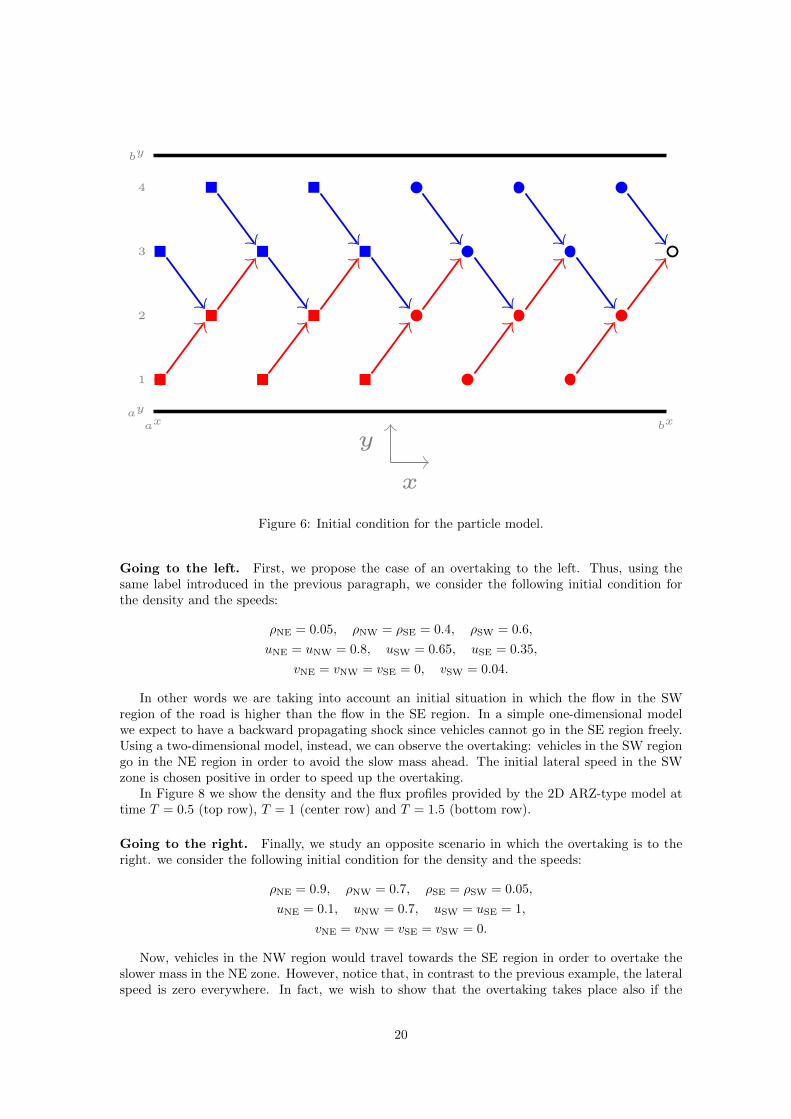
This situation is depicted in Figure 6 for the case of four lanes and it can be easily generalizedto the case of an arbitrary number of lanes. Dots and squares represent the vehicles on the road.More precisely, the red cars are in the first and second lane, traveling with a positive lateral speed(i.e., towards the left part of the road). Instead, the blue cars are in the third and fourth lane,traveling with a negative lateral speed (i.e., towards the left part of the road). The squares andthe dots identify the vehicles having speed 0.05 and 0.8 in x-direction, respectively. The arrowsshow, for each car, the interacting vehicle. The empty black circle is the “ghost” car, i.e. theboundary condition, which is necessary to compute the microscopic states of the last cars in lane 2and 4. The positions and the speeds of the ghost car are updated at each time using the positionsand the speeds of the last car in the same lane, i.e. the third one.

In Figure 7 we show the density and the fluxes profiles at Tfin = 0.1 provided by the macroscopicmodel. The time step is chosen according to the CFL condition. We consider a small final time inorder to guarantee that, in the particle model, vehicles remain in their part of the domain givenat initial time. At each time step the density around each car is computed again using equation(7) and for each car the interacting vehicle is chosen by (9). The values of the density aroundeach car and of the fluxes provided by the particle model are showed with red ∗-symbols. Wenotice that the microscopic and the macroscopic model seems to produce the same profiles at finaltime. Moreover, the density has the same decrease in the center of the road as observed in the 1Dsimulation, see Figure 1. This happens because the initial condition in x is similar to that givenin Section 2. Finally, we observe that the density tends to 0 in the left-most and in the right-mostpart of the road because of the initial condition on the lateral velocity which assumes that theflow is going towards the center part of the road.

The following two examples regard only the macroscopic model with the aim of showing thatit reproduces typical traffic flow situations, as an overtaking scenario.

19

y

x

bxaxay

by

1

2

3

4

Figure 6: Initial condition for the particle model.

Going to the left. First, we propose the case of an overtaking to the left. Thus, using thesame label introduced in the previous paragraph, we consider the following initial condition forthe density and the speeds:

ρNE = 0.05, ρNW = ρSE = 0.4, ρSW = 0.6,

uNE = uNW = 0.8, uSW = 0.65, uSE = 0.35,

vNE = vNW = vSE = 0, vSW = 0.04.

In other words we are taking into account an initial situation in which the flow in the SWregion of the road is higher than the flow in the SE region. In a simple one-dimensional modelwe expect to have a backward propagating shock since vehicles cannot go in the SE region freely.Using a two-dimensional model, instead, we can observe the overtaking: vehicles in the SW regiongo in the NE region in order to avoid the slow mass ahead. The initial lateral speed in the SWzone is chosen positive in order to speed up the overtaking.

In Figure 8 we show the density and the flux profiles provided by the 2D ARZ-type model attime T = 0.5 (top row), T = 1 (center row) and T = 1.5 (bottom row).

Going to the right. Finally, we study an opposite scenario in which the overtaking is to theright. we consider the following initial condition for the density and the speeds:

ρNE = 0.9, ρNW = 0.7, ρSE = ρSW = 0.05,

uNE = 0.1, uNW = 0.7, uSW = uSE = 1,

vNE = vNW = vSE = vSW = 0.

Now, vehicles in the NW region would travel towards the SE region in order to overtake theslower mass in the NE zone. However, notice that, in contrast to the previous example, the lateralspeed is zero everywhere. In fact, we wish to show that the overtaking takes place also if the

20

Figure 7: Density ρ (top-left), flux ρu (top-right) and flux ρv (bottom-center) profiles at timeTfin = 0.1 provided by the two-dimensional second-order macroscopic model (20). The red ∗-symbols shows the values of the density around each car and of the fluxes provided by the two-dimensional microscopic model (15).

initial lateral speed is zero. The macroscopic equations force the lateral speed of vehicle being inthe NW region to become negative and thus cars can overtake and travel in the right part of theroad.

In Figure 9 we show the density and the flux profiles provided by the 2D ARZ-type model attime T = 0.5 (top row), T = 1 (center row) and T = 1.5 (bottom row).

7 Concluding remarks

This paper introduced a 2D extension of the Aw-Rascle-Zhang [4, 19] second order model of trafficflow. The proposed model is rather simplistic and it can be viewed as a preliminary step towardsmulti-lane traffic modeling using 2D second order models. Nonetheless, it enables to capturetraffic dynamics caused by lane changing maneuvers and it complies with the desirable anisotropicfeature of vehicular traffic flow since the the maximum speed of the vehicles never exceeds thewave speed.

Hence, the proposed model opens many perspectives for future research toward several di-rections. In order to calibrate and test thoroughly the model enough real data on the trafficmacroscopic variables are required. We plan in future work to address this issue again and hopeto provide a rigorous validation of the model. Furthermore, the introduction of stochastic featuresin the lane-changing occurrence, derived from real data, is worth investigating. Finally, a moredetailed study on the analytical properties of the model could be provided.

21

Figure 8: Density ρ (left column), flux ρu (center column) and flux ρv (right column) profilesprovided by the two-dimensional second-order macroscopic model (20) at time Tfin = 0.5 (toprow), Tfin = 1 (center row) and Tfin = 1.5 (bottom row).

Acknowledgment

This work has been supported by HE5386/13-15 and DAAD MIUR project. We also thank theISAC institute at RWTH Aachen, Prof. M. Oeser, MSc. A. Fazekas and MSc. F. Hennecke forkindly providing the trajectory data.

References

[1] S. Al-nasur, New Models for Crowd Dynamics and Control, PhD thesis, Faculty of theVirginia Polytechnic Institute and State University, 2006.

[2] S. Al-nasur and P. Kachroo, A microscopic-to-macroscopic crowd dynamic model, inIEEE Conference on Intelligent Transportation Systems, 2006, pp. 606–611.

[3] A. Aw, A. Klar, T. Materne, and M. Rascle, Derivation of continuum traffic flowmodels from microscopic follow-the-leader models, SIAM J. Appl. Math., 63 (2002), pp. 259–278.

[4] A. Aw and M. Rascle, Resurrection of “second order” models of traffic flow, SIAM J. Appl.Math., 60 (2000), pp. 916–938 (electronic).

[5] C. Chalons and P. Goatin, Transport-equilibrium schemes for computing contact discon-tinuities in traffic flow modeling, Comm. Math. Sci., 5 (2007), pp. 533–551.

22

Figure 9: Density ρ (left column), flux ρu (center column) and flux ρv (right column) profilesprovided by the two-dimensional second-order macroscopic model (20) at time Tfin = 0.5 (toprow), Tfin = 1 (center row) and Tfin = 1.5 (bottom row).

[6] C. F. Daganzo, A behavioral theory of multi-lane traffic low part i: long homogeneousfreeway section, Transport. Res. B-Meth., 36 (2002), pp. 131–158.

[7] M. Di Francesco, S. Fagioli, and M. D. Rosini, Many particle approximation of theaw-rascle-zhang second order model for vehicular traffic, Mathematical Biosciences and En-gineering, 14 (2017), pp. 127–141.

[8] S. Fan, M. Herty, and B. Seibold, Comparative model accuracy of a data-fitted generalizedAw-Rascle-Zhang model, Netw. Heterog. Media., 9 (2014), pp. 239–268.

[9] K. A. Greenberg, J. M. and M. Rascle, Congestion on multilane highways, SIAM J.Appl. Math., 63 (2003), pp. 813–818.

[10] M. Herty and G. Visconti, A two-dimensional data-driven model for trafficflow on high-ways, 2017. Submitted. arXiv:1706.07965.

[11] E. Holland and A. Woods, A continuum model for the dispersion of traffic on two-laneroads, Transport. Res. B-Meth., 31 (1997), pp. 473–485.

[12] J. Laval and C. F. Daganzo, Lane-changing in traffic streams, Transport. Res. B-Meth.,40 (2006), pp. 251–264.

[13] C. E. Lawrence, Partial differential equations, American Mathematical Society, 2010.

23

[14] P. D. Lax, Hyperbolic systems of conservation laws and the mathematical theory of shockwaves, SIAM, 1973.

[15] M. J. Lighthill and G. B. Whitham, On kinematic waves. II. A theory of traffic flow onlong crowded roads, Proc. Roy. Soc. London. Ser. A., 229 (1955), pp. 317–345.

[16] B. D. Michalopoulos, P.G. and Y. Yamauchi, Multilane traffic dynamics: some macro-scopic considerations, Transport. Res. B-Meth., 18 (1984), pp. 377–395.

[17] P. I. Richards, Shock waves on the highway, Operations Res., 4 (1956), pp. 42–51.

[18] B. Seibold, M. R. Flynn, A. R. Kasimov, and R. R. Rosales, Constructing set-valuedfundamental diagrams from jamiton solutions in second order traffic models, Netw. Heterog.Media, 8 (2013), pp. 745–772.

[19] H. M. Zhang, A non-equilibrium traffic model devoid of gas-like behavior, Transport. Res.B-Meth., (2002), pp. 275–290.

24