liquidity issues in the u.s. natural gas market: part 1 of 2 47_65 wint… · natural gas (lng)....

J.P. Morgan Center for Commodities at the University of Colorado Denver Business School

GLOBAL COMMODITIES APPLIED RESEARCH DIGEST | Research Council Corner | www.jpmcc-gcard.com | Winter 2019

47

Liquidity Issues in the U.S. Natural Gas Market: Part 1 of 2 Gary Mahrenholz, Ph.D. Economist, Office of Enforcement’s Division of Energy Market Oversight, U.S. Federal Energy Regulatory Commission (FERC) Vincent Kaminski, Ph.D. Professor in the Practice of Energy Management, Jesse H. Jones Graduate School of Business, Rice University; and Member of the J.P. Morgan Center for Commodities’ (JPMCC’s) Research Council at the University of Colorado Denver Business School

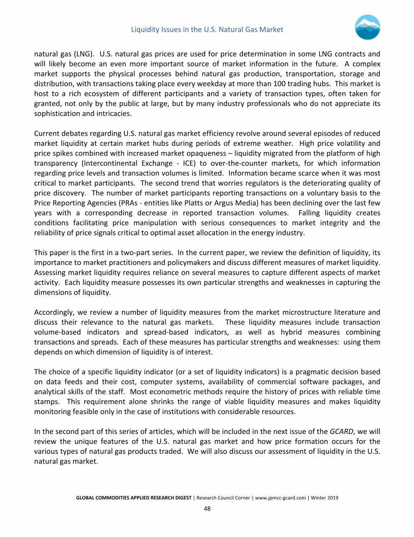
Professor Vince Kaminski, Ph.D., Rice University, and member of the J.P. Morgan Center for Commodities’ (JPMCC’s) Research Council, presenting at the JPMCC’s 2nd International Commodities Symposium, which was held at the University of Colorado Denver Business School in August 2018.

Introduction Natural gas is a commodity of critical importance to U.S. economic prosperity, as well as energy and national security. It accounted for about 28% of primary energy consumed in the United States in 2017, and about 32% of electricity generated in the same year. It was also used for heating, heating water and cooking in 86 million of the nation’s homes. A network of 300,000 miles of pipelines and 1,300,000 miles of distribution mains help to deliver natural gas every day. In recent years, the U.S. has become the biggest producer of natural gas in the world and will soon be an important exporter of liquefied

Liquidity Issues in the U.S. Natural Gas Market


48

natural gas (LNG). U.S. natural gas prices are used for price determination in some LNG contracts and will likely become an even more important source of market information in the future. A complex market supports the physical processes behind natural gas production, transportation, storage and distribution, with transactions taking place every weekday at more than 100 trading hubs. This market is host to a rich ecosystem of different participants and a variety of transaction types, often taken for granted, not only by the public at large, but by many industry professionals who do not appreciate its sophistication and intricacies. Current debates regarding U.S. natural gas market efficiency revolve around several episodes of reduced market liquidity at certain market hubs during periods of extreme weather. High price volatility and price spikes combined with increased market opaqueness – liquidity migrated from the platform of high transparency (Intercontinental Exchange - ICE) to over-the-counter markets, for which information regarding price levels and transaction volumes is limited. Information became scarce when it was most critical to market participants. The second trend that worries regulators is the deteriorating quality of price discovery. The number of market participants reporting transactions on a voluntary basis to the Price Reporting Agencies (PRAs - entities like Platts or Argus Media) has been declining over the last few years with a corresponding decrease in reported transaction volumes. Falling liquidity creates conditions facilitating price manipulation with serious consequences to market integrity and the reliability of price signals critical to optimal asset allocation in the energy industry. This paper is the first in a two-part series. In the current paper, we review the definition of liquidity, its importance to market practitioners and policymakers and discuss different measures of market liquidity. Assessing market liquidity requires reliance on several measures to capture different aspects of market activity. Each liquidity measure possesses its own particular strengths and weaknesses in capturing the dimensions of liquidity. Accordingly, we review a number of liquidity measures from the market microstructure literature and discuss their relevance to the natural gas markets. These liquidity measures include transaction volume-based indicators and spread-based indicators, as well as hybrid measures combining transactions and spreads. Each of these measures has particular strengths and weaknesses: using them depends on which dimension of liquidity is of interest. The choice of a specific liquidity indicator (or a set of liquidity indicators) is a pragmatic decision based on data feeds and their cost, computer systems, availability of commercial software packages, and analytical skills of the staff. Most econometric methods require the history of prices with reliable time stamps. This requirement alone shrinks the range of viable liquidity measures and makes liquidity monitoring feasible only in the case of institutions with considerable resources. In the second part of this series of articles, which will be included in the next issue of the GCARD, we will review the unique features of the U.S. natural gas market and how price formation occurs for the various types of natural gas products traded. We will also discuss our assessment of liquidity in the U.S. natural gas market.



49

We will now turn to introducing the general concept of market liquidity before considering a number of alternative measures of this concept, including their relevance to the natural gas market. Definition of Market Liquidity Market Liquidity: Financial Markets Liquidity is as important to financial and physical commodity markets as lubrication is to an engine. Decreasing market liquidity is a manifestation of a financial and economic crisis and a factor that may aggravate the crisis by extending it and deepening it through complicated feedback loops. This explains why market liquidity has received a lot of attention from academic economists and trading professionals. Most papers published in the scientific journals revolve around different aspects of liquidity in financial instruments with limited attention paid to the physical commodity markets. This is not surprising – commodity price information is fairly limited and modeling of the price formation processes requires understanding of the unique features of each specific commodity as well as the physical layer of the industry. This two-part series of articles covers the market liquidity issues as identified by the authors in the U.S. physical natural gas markets. Our articles are a work in progress and the authors hope that feedback from researchers and practitioners will help in completing this effort. Market liquidity is one of the most elusive concepts in finance.1 Its importance has been recognized by both market practitioners and economists who agree that defining and measuring liquidity is a work in progress:

“Liquidity is the lifeblood of financial markets. Its adequate provision is critical for the smooth operation of an economy. Its sudden erosion in even a single market segment or in an individual instrument can stimulate disruptions that are transmitted through increasingly interdependent and interconnected financial markets worldwide. Despite its importance, problems in measuring and monitoring liquidity risk persist.” (Fernandez, 1999).

In an International Monetary Fund (IMF) paper, Lybek and Sarr (2002) offer the following definition for market liquidity:

“Liquidity measures can be classified into four categories: (i) transaction cost measures that capture costs of trading financial assets and trading frictions in secondary markets; (ii) volume-based measures that distinguish liquid markets by the volume of transactions compared to the price variability, primarily to measure breadth and depth; (iii) equilibrium price-based measures that try to capture orderly movements towards equilibrium prices to mainly measure resiliency; and (iv) market-impact measures that attempt to differentiate between price movements due [to] the degree of liquidity from other factors ... No single measure, however, unequivocally measures tightness, immediacy, depth, breadth, and resiliency.”

The challenge of defining and measuring market liquidity arises from its multidimensional character – it is defined by listing a number of market attributes, enumerated in the IMF paper quoted above, such as transaction volumes, transaction costs and the time required to execute a transaction, which often



50

change in different directions. The most frequently repeated definition of liquidity is the ability to transact in large volumes, over short periods of time, without (or with limited) price impact, and at low transaction costs.2 Often these objectives conflict as a market participant has to accept trade-offs between the volume and the speed of a trade and the cost of executing that transaction. Increasing transaction volume may require trading over a longer time period, waiting for additional traders to enter the market, or making price concessions to exhaust more quickly the bid / offer stack. Price concessions will be reflected in a higher market impact of a specific set of transactions. Perceptions of market liquidity depend on which of those different characteristics are important to a market participant. Liquidity, like beauty, is in the eye of the beholder. This explains why the definition of liquidity and its measure cannot be compressed into one sentence or one magic formula. The holistic assessment of market liquidity requires use of multiple indexes which shine light on many different aspects of market activity. The importance and usefulness of these indexes will vary from market to market and from time period to time period. Sometimes the inability to calculate one or several measures of liquidity (discussed below) is the best indicator of extreme market conditions. It is important to distinguish between market liquidity and funding liquidity as these two issues are often conflated and tend to interact, especially under conditions of economic distress. Funding liquidity corresponds to the ability to obtain access to cash (or cash equivalents such as credit lines) on short notice. Market illiquidity can exacerbate funding illiquidity as a firm may find it difficult to reduce inventories, liquidate certain assets and may face increased costs of acquisition of materials required to carry on its business activities. Funding illiquidity may force potential counterparties to reduce their trading activities and even withdraw completely from the market. U.S. energy industry practitioners still have vivid memories of the paralyzed natural gas and electricity markets in 2002 and 2003, following the Enron bankruptcy. The definitions of market liquidity available in the economic literature have been developed for the financial markets and, therefore, cannot be mechanically applied to physical energy. Financial instruments can be created and distributed, ignoring physical constraints of the system and exist as records in data servers. In the case of physical energy, trading requires access to the production and distribution infrastructure as uninterrupted flows of commodities between producers and end-users are the overriding concern and the yardstick by which the markets are assessed. A more appropriate definition of liquidity in this case is the ability of the market to absorb supply/demand shocks and keep the proverbial lights on. Other elements of the definition of market liquidity mentioned above are secondary in their importance to the overriding objective of system resiliency. The Importance of Market Liquidity Market liquidity, the ability to transact on a short notice, at required levels, and at reasonable cost, is important not just for the convenience of the traders. Liquid and transparent markets are a public good with a positive impact on the overall efficiency of the national economy. To explain this one has to distinguish between physical and financial energy markets.



51

Liquidity of physical energy markets helps to increase the resilience of the supply chain to demand/supply shocks caused by extreme weather events and forced outages of power generation plants, natural gas pipelines and high voltage transmission lines. For example, an outage of a nuclear power plant triggers a chain of market transactions and physical operations such as the start-up of idle power plants (or expanding output from power plants already in operation), purchases of additional fuel, wheeling electricity from other areas, and extraction of natural gas from storage. In the absence of an efficient market, such operations would be either impossible or time consuming and expensive, and this would in turn result in cascading disruptions of multiple supply chains, affecting many industrial, commercial and residential end users of electricity, declarations of force majeure, and costly legal disputes. Liquidity of financial energy markets makes a contribution to the national economy through transfer of risks, accomplished through hedging and insurance-like transactions.3 Availability of hedging instruments insulates energy companies from the consequences of extreme events, reduces the risk of cash shortfalls and suppresses volatility of earnings. This in turn translates into a lower cost of debt, the enhanced ability to fund investment projects and the ability to concentrate on long-term operational challenges. The cost of hedging instruments varies positively with market volatility4 which is one manifestation of low liquidity. This is another example how lack of liquidity translates into a higher cost of doing business for the producers and the end users of energy. Low market liquidity is often associated with the potential for market manipulation as relatively small transaction volumes may be associated with significant market impact. Market manipulation undermines confidence in the price system and impedes development of the market for energy related derivatives used for risk management. Derivative contracts are usually cash settled and market participants are reluctant to enter into such contracts if they cannot trust the integrity of the prices used for settlements. Measuring Market Liquidity Market microstructure theorists developed several benchmarks for measuring market liquidity and tracking it over time. The benchmarks can be classified based on the type of market information used in their calculation and include:

1. Transaction volume-based indicators; 2. Spread-based indicators; 3. Transaction flow-based indicators; and 4. Hybrid indicators.

This classification can be further refined by considering the granularity of available data:

1. Benchmarks based on the order book information and/or high frequency data; and 2. Benchmarks based on volume and price data recorded at low frequency (hourly or daily).



52

The first group of benchmarks relies on high frequency transaction data and bid/offer information for both consummated and unconsummated transactions which are not available for most energy markets. The second group of benchmarks is based on lower frequency (mostly daily) closing prices and aggregate volumes. As indicated above, different measures of market liquidity should be used jointly and assessed using judgment and insights derived from experience, as no single index captures all the dimensions of market conditions at one point in time. The trends are often more important than the specific readings of a given indicator. The inability to calculate one or more of the benchmarks (1) – (4) on the previous page may be the best evidence of extreme market illiquidity.5 Our survey of liquidity measures will describe three of these benchmarks: transaction volume-based indicators, spread-based indicators, and hybrid indicators, including their respective applications to the natural gas market. Transaction Volume - Based Indicators Market liquidity indicators reflecting the level of trading activity are as follows:

1. Transaction volume per unit of time; 2. The number of market participants trading in a given market; 3. The number of transactions per unit of time; 4. Time elapsed between two successive transactions; and 5. Average transaction size.

Transaction volume, the number of transactions and the number of counterparties present at the market at a given time period are the most obvious and intuitive measures of market liquidity. The appeal of these measures is to a large extent based on the availability of empirical data for most markets (free of charge or available at a fee) and the ease of calculating and reporting relevant statistics without recourse to complicated quantitative models. Transaction volume is calculated as: 𝑉𝑉𝑉𝑉𝑉𝑉𝑡𝑡 = ∑ 𝑣𝑣𝑉𝑉𝑉𝑉𝑖𝑖

𝑛𝑛𝑡𝑡𝑖𝑖=1 (1)

where voli denotes the volume of transaction i, nt – the number of transactions in time period t. In the case of energy markets, transaction volume information available to the public varies from market to market. For example, in the case of the U.S. natural gas and electricity markets, daily volume of Intercontinental Exchange (ICE) transactions used in the calculation of the day-ahead price index (physical transactions) is available from the exchange. The volume is reported as an aggregate daily number with no information about individual underlying transactions. High granularity data may be purchased from the exchange or obtained by the traders by scraping the ICE screens.



53

The turnover measure combines physical volume information with price information: 𝑉𝑉𝑡𝑡 = ∑ 𝑣𝑣𝑉𝑉𝑉𝑉𝑖𝑖 × 𝑝𝑝𝑖𝑖

𝑛𝑛𝑡𝑡𝑖𝑖=1 (2)

where pi denotes the price at which the ith transaction took place. The volume and turnover indicators are sometimes reported as volume (turnover) duration, the inverse of the volume (turnover) per unit of time (Gouriéroux et al., 1999). The latter measure indicates the time required to trade a certain volume (or to reach a certain turnover level.) Churn factor is defined as the ratio of transaction volume to actual physical deliveries. In other words, this is the number of times each molecule, barrel or electron is re-traded in the market before reaching the final user. The difficulty in calculating the churn factor is related to estimating actual volume underlying a given market and defining the final users. Churn factors are used in European natural gas markets where physical configuration of trading hubs makes determination of actual deliveries easier than in the case of the highly complex U.S. natural gas transportation and distribution network. According to Heather and Petrovich (2017) in an Oxford Institute for Energy Studies paper:

“Commodity markets are deemed to have reached maturity when the churn is in excess of 10 times. In this one metric all others are, necessarily, reflected: if there are many participants, trading many different products in large quantities, then the churn rate is likely to be high. The churn rate is used by traders as a ‘snapshot’ of a market’s liquidity; some traders will not participate in markets with a churn of less than 10 and many financial players will only participate when the churn is above 12 times.”

In 2016, the churn rate in two European natural gas hubs was above 10: 57.1 for TTF [Title Transfer Facility in the Netherlands – GM and VK] and 22.1 for NBP [National Balancing Point in the UK – GM and VK]. Other trading hubs had much lower churn ratios, ranging from 5.7 for CEGH/VTP [Central European Gas Hub AG (CEGH), located in Vienna, Austria, Virtual Trading Point – GM and VK] to 0.1 for PVB [Spanish Punto Virtual de Balance – GM and VK]. The threshold churn level of 10 is rather arbitrary. It seems that market participants learn through experience to establish a certain intuitive confidence level of trading intensity in specific commodity markets, and this can vary by commodity and over time and location. The U.S. market consists of a network of interconnected pipelines with no obvious, well-defined boundaries of different regions. Since the churn index in the U.S. market is difficult to estimate, given its largely reticulated nature, measuring liquidity using a variety of benchmarks is a useful alternative in attempting to ascertain how liquidity varies by natural gas hub.



54

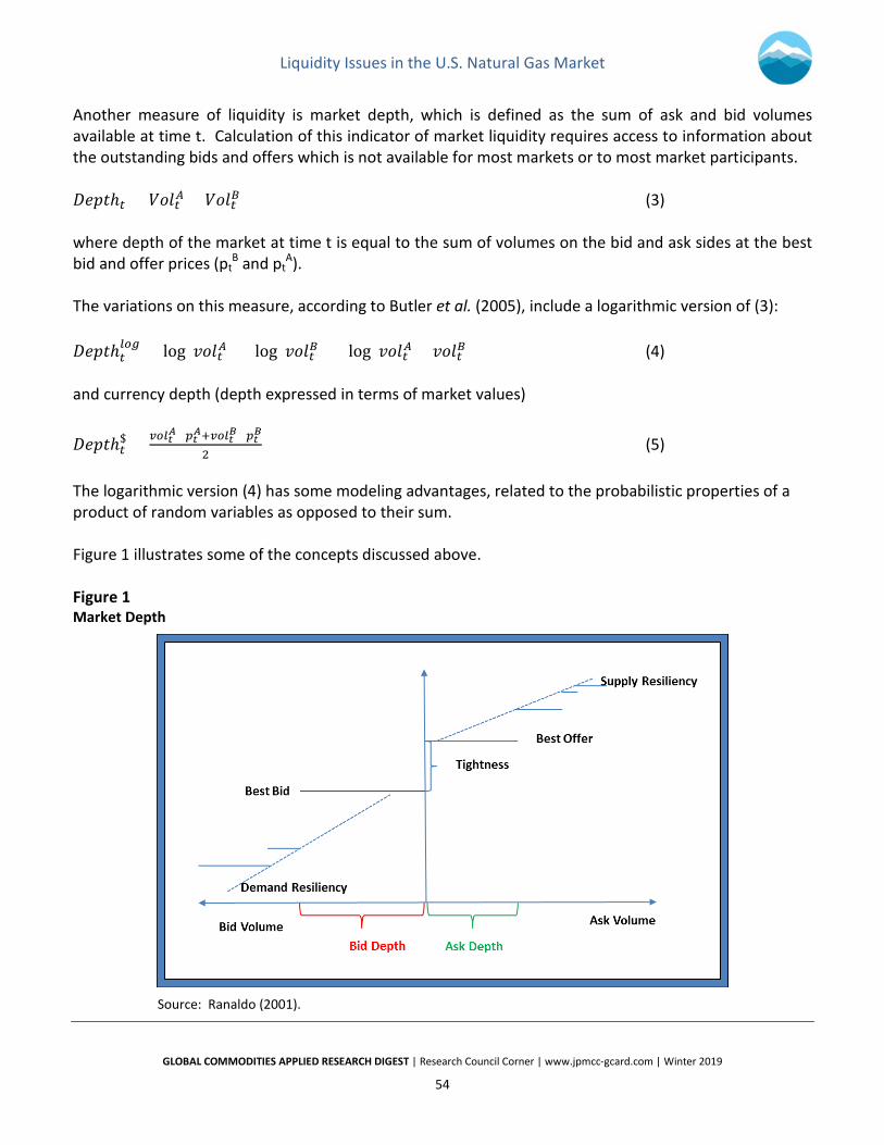
Another measure of liquidity is market depth, which is defined as the sum of ask and bid volumes available at time t. Calculation of this indicator of market liquidity requires access to information about the outstanding bids and offers which is not available for most markets or to most market participants. 𝐷𝐷𝐷𝐷𝑝𝑝𝐷𝐷ℎ𝑡𝑡 = 𝑉𝑉𝑉𝑉𝑉𝑉𝑡𝑡𝐴𝐴 + 𝑉𝑉𝑉𝑉𝑉𝑉𝑡𝑡𝐵𝐵 (3) where depth of the market at time t is equal to the sum of volumes on the bid and ask sides at the best bid and offer prices (pt

B and ptA).

The variations on this measure, according to Butler et al. (2005), include a logarithmic version of (3): 𝐷𝐷𝐷𝐷𝑝𝑝𝐷𝐷ℎ𝑡𝑡

𝑙𝑙𝑙𝑙𝑙𝑙 = log(𝑣𝑣𝑉𝑉𝑉𝑉𝑡𝑡𝐴𝐴) + log(𝑣𝑣𝑉𝑉𝑉𝑉𝑡𝑡𝐵𝐵) = log(𝑣𝑣𝑉𝑉𝑉𝑉𝑡𝑡𝐴𝐴 × 𝑣𝑣𝑉𝑉𝑉𝑉𝑡𝑡𝐵𝐵) (4) and currency depth (depth expressed in terms of market values)

𝐷𝐷𝐷𝐷𝑝𝑝𝐷𝐷ℎ𝑡𝑡$ = 𝑣𝑣𝑙𝑙𝑙𝑙𝑡𝑡𝐴𝐴×𝑝𝑝𝑡𝑡𝐴𝐴+𝑣𝑣𝑙𝑙𝑙𝑙𝑡𝑡𝐵𝐵×𝑝𝑝𝑡𝑡𝐵𝐵

2 (5)

The logarithmic version (4) has some modeling advantages, related to the probabilistic properties of a product of random variables as opposed to their sum. Figure 1 illustrates some of the concepts discussed above. Figure 1 Market Depth

Source: Ranaldo (2001).



55

Limitations of Trading Volume as a Measure of Liquidity The volume of transactions can be a misleading measure of liquidity. One could argue that a vibrant, liquid market implies a large transaction volume and a large number of transactions, but the reverse statement is not necessarily true. The following example provides an illustration:

“On Kentucky Derby day, Bob and Joe invested in a barrel of beer and set off to Louisville with the intention of selling at the racetrack at a dollar a pint. On the way, Bob, who had one dollar left in the world, began to feel a great thirst, and drank a pint of beer, paying Joe the dollar. A little later, Joe yielded to the same desire, and drank a pint of beer, returning the dollar to Bob. The day was hot, and before long Bob was thirsty again, and so, a little later, was Joe. When they arrived at the track, the dollar was back in Bob’s pocket, but the beer was all gone.” (Robertson, 1922).

The beer market on this specific day seemed to be quite liquid (no pun intended) if assessed by the number of transactions. Transaction volumes may often reflect artificial activity triggered by many industry specific circumstances or macroeconomic conditions. A few examples from recent history illustrate how misleading volume can be if used as a measure of liquidity to the exclusion of other information. Enron’s early success, driven to a large extent by permissive mark-to-market accounting rules, enticed a number of merchant energy companies (producers, utilities, and midstream companies) to imitate the Houston company, proudly calling itself, “Wall Street away from Wall Street,” and enter the energy trading business (through the establishment of specialized, unregulated merchant units), resulting in the creation of a machinery with a scale that exceeded industry needs. The merchant energy companies were chasing relatively immature markets with capacity insufficient to justify the size of the trading operations they had set up, driven by excessively optimistic expectations of market growth. The outcome was a daisy chain of transactions between marketing companies, inserting themselves between end users and producers, often with as many as twenty intermediate steps before molecules and electrons reached final destinations. Given that the volume of transactions became one of the valuation metrics for start-up energy trading firms, in lieu of non-existing profits, some companies sought to artificially inflate their portfolios by engaging in the so-called round trips (wash trades), nearly simultaneous purchases and sales, under identical or almost identical terms. A well-known example is the case of circular trades between Reliant and Enron executed on the platform EnronOnLine in January of 2001.6 The number of transactions during a given time period may be equally misleading. A large number of transactions in a given time window is usually considered a manifestation of market liquidity, but this is not always the case. In an illiquid market a trader has to “work the trade,” by splitting the transaction into smaller installments in order to avoid detection by predatory traders, who can front run her, and to reduce the market impact of her trades. Some traders wish to execute a transaction in one discrete, big step. For example, a trader buying natural gas for storage injection or selling gas withdrawn from storage does not want to overwhelm the back office, schedulers and accountants with multiple deals,



56

executed at different price levels, requiring multiple time-consuming confirmations and ledger entries. One-stop shopping may be accomplished by offering price concessions to her counterparties.7 Trading volumes may also be inflated for other reasons, related to cyclicality inherent in the activities of the financial industry. Spread-Based Liquidity Measures The logic behind spread-based liquidity measures is very simple: low levels of market liquidity translate into wider spreads between bid and offer prices. The market participants who want to transact have to compensate their counterparties for increased risk. A liquidity provider accommodating a potential buyer (seller) recognizes that in an illiquid market closing the position, i.e., entering into an offsetting transaction, may take time (with a higher risk of a potentially adverse market movement) or may require making price concessions. A higher bid-offer spread is compensation for taking this risk. In many markets, bid-offer spreads are not observable or are not available to most market participants. The good news is that bid-offer spreads (as documented later in this paper) can be estimated from the consummated transaction prices, as long as the price history is available with reliable time stamps (i.e., the transaction prices can be sorted in chronological order.) Bid-Ask Spreads Effective Spread is defined as: 𝐸𝐸𝐸𝐸 = 2 × | ln(𝑃𝑃𝑖𝑖) − ln(𝑀𝑀𝑖𝑖)| (6) where Pi stands for the price at which the ith transaction was executed and Mi is the midpoint price at the time of the ith transaction. In the financial literature, this spread is often referred to as the TAQ spread after the name of the database Trade and Quote, containing stock market transaction data for NYSE, NASDAQ and regional exchanges.8 Effective spread is reported as a volume-weighted average over a certain time period (typically a month.) In Huang and Stoll (1996), realized half-spread is defined as:

𝑅𝑅𝑅𝑅𝐸𝐸 = 𝑃𝑃𝑡𝑡+𝜏𝜏 − 𝑃𝑃𝑡𝑡|𝑃𝑃𝑡𝑡 = 𝑝𝑝𝑡𝑡𝐵𝐵 (7) 𝑅𝑅𝑅𝑅𝐸𝐸 = −(𝑃𝑃𝑡𝑡+𝜏𝜏 − 𝑃𝑃𝑡𝑡)|𝑃𝑃𝑡𝑡 = 𝑝𝑝𝑡𝑡𝐴𝐴 (8)

where pB

t (pAt) denotes the bid (ask) price at time t, Pt (Pt+τ) denotes price at time t (t+ τ), where τ

denotes a chosen time interval (usually a minute or five minutes.) The expression Pt = pBt (Pt = pA

t) means that the transaction was executed at the bid (ask) price. In other words, the transaction was either a sell or a buy (a seller or a buyer initiated.) The symbol “|” means that the definition of realized half spread is conditional on the transaction type.



57

Some recent papers use a modified definition of realized spread: 𝑅𝑅𝐸𝐸 = 2 × (ln (𝑃𝑃𝑡𝑡+𝜏𝜏) − ln (𝑃𝑃𝑡𝑡))|𝑃𝑃𝑡𝑡 = 𝑝𝑝𝑡𝑡𝐵𝐵 (9) 𝑅𝑅𝐸𝐸 = −2 × (ln (𝑃𝑃𝑡𝑡+𝜏𝜏) − ln (𝑃𝑃𝑡𝑡))|𝑃𝑃𝑡𝑡 = 𝑝𝑝𝑡𝑡𝐴𝐴 (10) The direction of the trade (buys vs. sells) is determined in practice using the algorithm proposed by Lee and Ready (1991).9 An alternative formulation for realized spread is called the Percent Realized Spread: 𝑃𝑃𝑅𝑅𝐸𝐸 = 2 × 𝑞𝑞𝑖𝑖(ln (𝑃𝑃𝑖𝑖) − ln (𝑀𝑀𝑖𝑖+5)) (11) where Pi denotes the price of the ith trade, Mi+5 is the midpoint price 5 minutes after this trade occurs. The variable qi is an indicator variable that equals +1 if the ith trade is a buy and -1 if the ith trade is a sell. Percent Quoted Spread (PQS) is another indicator based on bid/offer time series: 𝑃𝑃𝑃𝑃𝐸𝐸 = 𝐴𝐴𝐴𝐴𝐴𝐴−𝐵𝐵𝑖𝑖𝐵𝐵

𝐴𝐴𝐴𝐴𝐴𝐴+𝐵𝐵𝐵𝐵𝐵𝐵2

(12)

where Ask is the best ask quote at a given time window, and Bid is the best bid quote. The PQS indicator is reported as the time-weighted average of indicators calculated for each time window. Roll Index and Extensions Roll (1984) proposed a method of estimating the effective spread, s, from low frequency price data. This paper demonstrated that the following relationship holds: 𝐶𝐶𝑉𝑉𝑣𝑣(∆𝑃𝑃𝑡𝑡,∆𝑃𝑃𝑡𝑡−1) = 1

4𝑠𝑠2 (13)

𝑠𝑠 = 2�−𝐶𝐶𝑉𝑉𝑣𝑣(∆𝑃𝑃𝑡𝑡,∆𝑃𝑃𝑡𝑡−1) (14) 𝑠𝑠 = 0 𝑖𝑖𝑖𝑖 𝐶𝐶𝑉𝑉𝑣𝑣(∆𝑃𝑃𝑡𝑡,∆𝑃𝑃𝑡𝑡−1) > 0 (15) In equation (13), ∆Pt stands for the price increment from period to period, and ∆Pt-1 is the price increment lagged by one period.10 Cov(∆Pt, ∆Pt-1) stands for the covariance between the price increments. The covariance can be estimated using the Ordinary Least Squares (OLS) technique or directly from its definition. Hasbrouck (2004) recommended using Bayesian regression techniques in place of OLS.11



58

It is assumed that s = 0 if the covariance is positive since the square root of a negative number in (14) cannot be calculated. One shortcoming of the original Roll index of liquidity is that the estimated spread would be equal to zero in many cases, which is not a very satisfying result. The model proposed by Roll was extended and modified by a number of economists who relaxed some of the assumptions of the original model or proposed different estimation techniques. Modification of the assumption of balanced order flow (equal probability of buy and sell orders) leads to a formula: 𝑠𝑠 = 𝐴𝐴𝑅𝑅

2�𝜂𝜂(1−𝜂𝜂) (16)

where sR stands for the spread calculated according to the Roll procedure and η stands for the probability of receiving a buy order. Relaxing the assumption that orders are not auto-correlated leads to the following formula for the spread: 𝑠𝑠 = 1

1−𝛿𝛿�−𝐶𝐶𝑉𝑉𝑣𝑣(∆𝑃𝑃𝑡𝑡,∆𝑃𝑃𝑡𝑡−1) (17)

where δ = Probability (dt+1 = dt). The assumption that orders carry information leads to an alternative formula for the bid/offer spread: 𝑠𝑠 = 2(𝜆𝜆 + 𝛾𝛾) (18) where λ and γ are estimated through a regression equation: Δ𝑃𝑃𝑡𝑡 = 𝜆𝜆𝑑𝑑𝑡𝑡 + 𝛾𝛾Δ𝑑𝑑𝑡𝑡 + 𝜀𝜀𝑡𝑡 (19) where λ captures the adverse selection spread component and γ represents the order processing cost fraction.



59

High/Low Prices Corwin and Schultz (2012) proposed a formula for estimating the bid/ask percentage spread from daily high and low prices. The percentage spread is given by: 𝐸𝐸 = 2(𝑒𝑒𝛼𝛼−1)

1+𝑒𝑒𝛼𝛼 (20)

where

𝛼𝛼 = �2𝛽𝛽−�𝛽𝛽3−2√2

− � 𝛾𝛾3−2√2

(21)

with

𝛽𝛽 = 𝔼𝔼{∑ [log �𝐻𝐻𝑡𝑡+𝑗𝑗𝐿𝐿𝑡𝑡+𝑗𝑗

�]2}1𝑗𝑗=0 (22)

𝛾𝛾 = [log �𝐻𝐻𝑡𝑡,𝑡𝑡+1𝐿𝐿𝑡𝑡,𝑡𝑡+1

�]2

(23)

where Ht (Lt) denotes high (low) price for day t. Ht,t+1 (Lt,t+1) denotes high (low price) over the period of two days. The symbol 𝔼𝔼 denotes expectation operator. Implementation of this formula in the case of energy markets requires a modification. Electricity prices may be negative and, if this is the case, natural logs are replaced with (H/L) - 1 terms under some circumstances.12 Thompson-Waller Spread Estimator As discussed in Thompson and Waller (1988) and in Bryant and Haigh (2002), the Thompson and Waller (TW) nominal bid/ask spread estimator is calculated as follows: 𝑇𝑇𝑇𝑇 = 1

𝑇𝑇∑ |∆𝑝𝑝𝑖𝑖|𝑇𝑇𝑖𝑖=1 (24)

where ∆pi stands for non-zero intraday price changes, and T stands for the number of observations. A modification of this index has been proposed by Wang et al. (1997). Their measure is referred to in the literature as the CFTC liquidity measure (as the CFTC was using this liquidity index at the time (1997).) This measure is similar to the TW index, except that they only use non-zero price changes of opposite direction. In other words, any price change that follows another price change of the same sign is ignored.



60

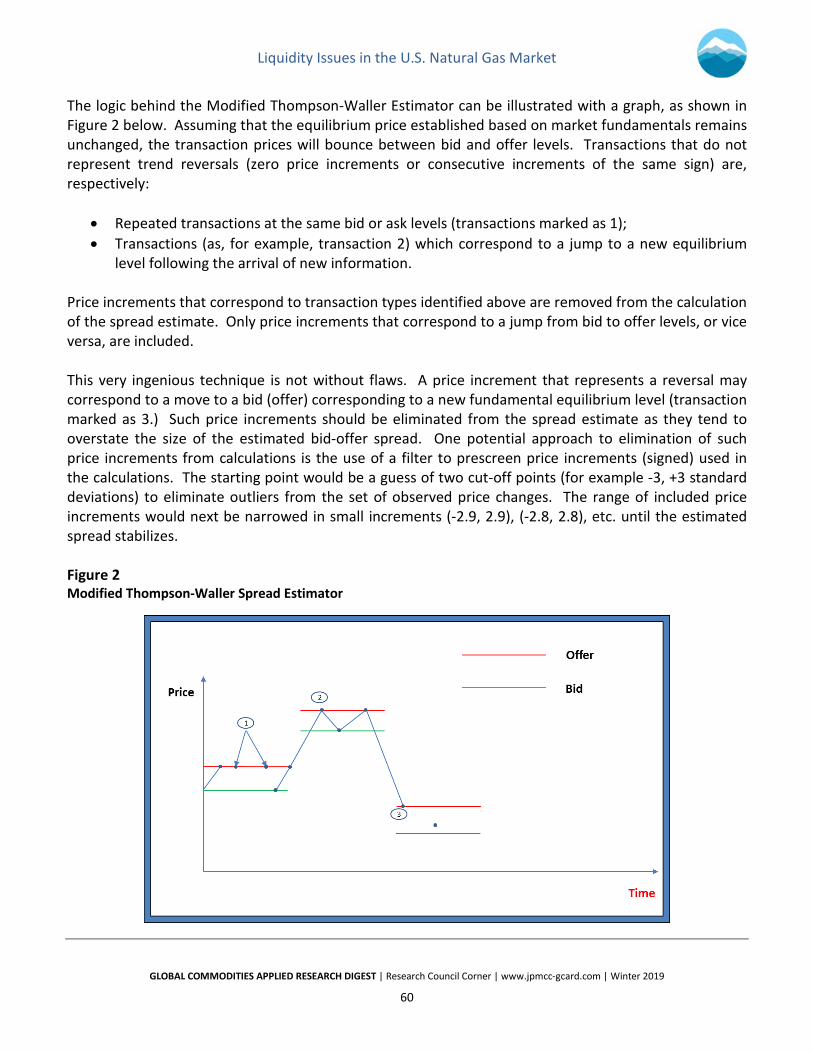
The logic behind the Modified Thompson-Waller Estimator can be illustrated with a graph, as shown in Figure 2 below. Assuming that the equilibrium price established based on market fundamentals remains unchanged, the transaction prices will bounce between bid and offer levels. Transactions that do not represent trend reversals (zero price increments or consecutive increments of the same sign) are, respectively:

• Repeated transactions at the same bid or ask levels (transactions marked as 1); • Transactions (as, for example, transaction 2) which correspond to a jump to a new equilibrium

level following the arrival of new information. Price increments that correspond to transaction types identified above are removed from the calculation of the spread estimate. Only price increments that correspond to a jump from bid to offer levels, or vice versa, are included. This very ingenious technique is not without flaws. A price increment that represents a reversal may correspond to a move to a bid (offer) corresponding to a new fundamental equilibrium level (transaction marked as 3.) Such price increments should be eliminated from the spread estimate as they tend to overstate the size of the estimated bid-offer spread. One potential approach to elimination of such price increments from calculations is the use of a filter to prescreen price increments (signed) used in the calculations. The starting point would be a guess of two cut-off points (for example -3, +3 standard deviations) to eliminate outliers from the set of observed price changes. The range of included price increments would next be narrowed in small increments (-2.9, 2.9), (-2.8, 2.8), etc. until the estimated spread stabilizes. Figure 2 Modified Thompson-Waller Spread Estimator



61

Another shortcoming of the discussed estimator is that it is based on intuition and is not supported by assumptions about the stochastic process followed by the underlying price. This makes it impossible to deploy the usual artillery of statistical tests to assess the quality of the estimates. In spite of the shortcomings, the modified Thompson-Waller spread estimator is very popular among practitioners: it is easy to calculate, as long as transaction prices with reliable time stamps are available. The computational burden is low and the technique can be used for a large number of trading locations as well as for the analysis of intra-day liquidity patterns. A more complicated approach (for example, Bayesian regression techniques) would require a time-consuming review of regression printouts and an analysis of regression diagnostics. Hybrid Liquidity Measures Amihud (2002) provides a price impact measure that is given by 𝐼𝐼𝑉𝑉𝑉𝑉𝑖𝑖𝑞𝑞𝐼𝐼𝑖𝑖𝑑𝑑𝑖𝑖𝐷𝐷𝐼𝐼 = 𝐴𝐴𝑣𝑣𝐷𝐷𝐴𝐴𝐴𝐴𝐴𝐴𝐷𝐷( |𝑟𝑟𝑡𝑡|

𝑉𝑉𝑙𝑙𝑙𝑙𝑉𝑉𝑉𝑉𝑒𝑒𝑡𝑡) (25)

with rt being the price return on day t. The Amihud index is usually averaged or summed over monthly periods. Volume in equation (25) is replaced sometimes by turnover (Σpq) or the number of trades in a given time period. The absolute value of price return is, in some versions of this measure, replaced by the square of price increment (Pt – Pt-1). A related measure is the Amivest Liquidity ratio: 𝐿𝐿𝑖𝑖𝑞𝑞𝐼𝐼𝑖𝑖𝑑𝑑𝑖𝑖𝐷𝐷𝐼𝐼 = 𝐴𝐴𝑣𝑣𝐷𝐷𝐴𝐴𝐴𝐴𝐴𝐴𝐷𝐷(𝑉𝑉𝑙𝑙𝑙𝑙𝑉𝑉𝑉𝑉𝑒𝑒𝑡𝑡|𝑟𝑟𝑡𝑡| ) (26)

which is defined for non-zero return days. The logic behind Amihud’s index of liquidity is very simple, and this explains its popularity in applied financial economics. The value of the index increases with greater absolute return, i.e., greater market impact, for a given level of volume (turnover.) A higher value for Amihud’s index means that the market becomes more illiquid: the price reaction measured by the price return is stronger for a given transaction volume. An imputed round trip cost measure has been proposed by Dick-Nielsen et al. (2012). The intuition behind this measure is the observation that an asset (including in the energy markets) may trade two or three times in a short timeframe. This may happen when a dealer acts as a principal buying from one market participant, warehousing the risk for a short period of time, and selling the underlying to another party.



62

The imputed round trip cost (IRC) is defined as 𝐼𝐼𝑅𝑅𝐶𝐶 = 𝑃𝑃𝑚𝑚𝑚𝑚𝑚𝑚−𝑃𝑃𝑚𝑚𝐵𝐵𝑚𝑚

𝑃𝑃𝑚𝑚𝑚𝑚𝑚𝑚 (27)

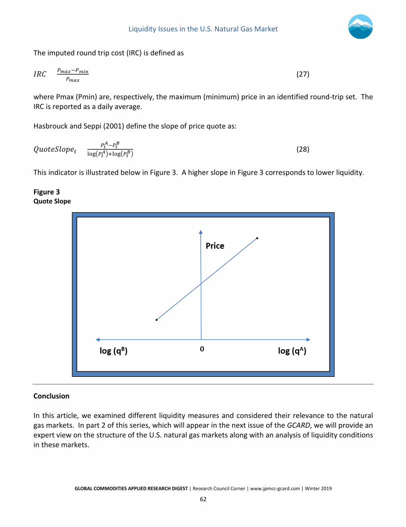
where Pmax (Pmin) are, respectively, the maximum (minimum) price in an identified round-trip set. The IRC is reported as a daily average. Hasbrouck and Seppi (2001) define the slope of price quote as:

𝑃𝑃𝐼𝐼𝑉𝑉𝐷𝐷𝐷𝐷𝐸𝐸𝑉𝑉𝑉𝑉𝑝𝑝𝐷𝐷𝑡𝑡 = 𝑃𝑃𝑡𝑡𝐴𝐴−𝑃𝑃𝑡𝑡𝐵𝐵

log�𝑃𝑃𝑡𝑡𝐴𝐴�+log�𝑃𝑃𝑡𝑡𝐵𝐵� (28)

This indicator is illustrated below in Figure 3. A higher slope in Figure 3 corresponds to lower liquidity. Figure 3 Quote Slope

Conclusion In this article, we examined different liquidity measures and considered their relevance to the natural gas markets. In part 2 of this series, which will appear in the next issue of the GCARD, we will provide an expert view on the structure of the U.S. natural gas markets along with an analysis of liquidity conditions in these markets.



63

Endnotes 1 As noted in Kay (2015), “the word [liquidity] is widely – almost obsessively – used in financial markets, but often without any precise or particular meaning. A casual search of investment dictionaries and encyclopedias for definitions of liquidity will reveal as many definitions as sources.” 2 Transaction costs are defined here as commissions, order confirmation and processing costs, taxes and fees. Sometimes the transaction cost definition is expanded by adding a market impact component. 3 Weather derivatives are an example of a hybrid instrument that combines the features of a derivative and an insurance product. A weather derivatives contract is not exactly an insurance product because the buyer does not have to provide a proof of a loss: the occurrence of a weather event is sufficient. 4 Volatility of prices is the most important input to option pricing models. 5 As pointed out in the literature, different measures of liquidity applied to the same market may produce significantly different results. This is why judgment and trend analysis are so critically important. 6 “On this day [January 31, 2001], 227 trades took place on EOL [EnronOnLine]; more than 75 percent of them were transactions between Reliant and Enron. […] The first transaction, at 8:00 a.m., is an Enron purchase of 10,000 MMBtu at $11.30/MMBtu. The last transaction, at 9:30 a.m., is a sale of 10,000 MMBtu from Reliant to Enron for $15/MMBtu. […] Prices rise slightly during the first hour of trading, from $11.30 to $12. Once Reliant begins actively churning, the price rises quickly and steadily, peaking at $15.30 and closing $3.70 higher than the price at which it opened.” (FERC, 2003). 7 Many traders that we have talked to note that large volume transactions related to storage management, pipeline balancing or power plant fuel acquisition are transacted bilaterally at prices based on a negotiated differential to currently observed ICE prices at a specific location. 8 According to the New York Stock Exchange, “[t]he dataset includes Daily NBBO File, Daily Quotes File, Daily TAQ Master File, Daily Trades File, Daily TAQ Quote Admin Message LULD, Daily TAQ Trade Admin Message LULD, and Daily TAQ CTA & Daily TAQ UTP Admin Messages.” NBBO stands for National Best Bid and Offer, LULD stands for Limit Up-Limit Down. As of June 10, 2019, current information on the dataset is available at https://www.nyse.com/market-data/historical/daily-taq. 9 The shortcomings of this algorithm are discussed in a number of papers, including in Theissen (2001) and in Ellis et al. (2000). 10 If t = 10, for example, ∆Pt would be the change in price between t = 10 and t = 9. The lagged price increment ∆Pt-1 would be the change in price between t = 9 and t = 8. 11 There are several software packages available to implement this approach, including the Markov Chain Monte Carlo procedure in SAS. 12 The natural logarithm of X/Y is roughly equal to X/Y-1, if X and Y do not differ too widely. The opinions expressed in this paper are solely the authors’, and do not necessarily represent the views of the United States, the Federal Energy Regulatory Commission as a whole, any individual Commissioner, or Commission staff. References Amihud, Y., 2002, “Illiquidity and Stock Returns: Cross-Section and Time Series Effects,” The Journal of Financial Markets, Vol. 5, No. 1, January, pp. 31-56.

https://www.nyse.com/market-data/historical/daily-taq



64

Bryant, H. and M. Haigh, 2002, “Bid-Ask Spreads in Commodity Futures Markets,” The University of Maryland, Working Paper 02-07. Butler, A., Grullon, G. and J. Weston, 2005, “Stock Market Liquidity and the Cost of Issuing Equity,” The Journal of Financial and Quantitative Analysis, Vol. 40, No. 2, June, pp. 331-348. Corwin, S. and P. Schultz, 2012, “A Simple Way to Estimate Bid-Ask Spreads from Daily High and Low Prices,” The Journal of Finance, Vol. 67, No. 2, April, pp. 719–759. Dick-Nielsen, J., Feldhütter, P. and D. Lando, 2012, “Corporate Bond Liquidity Before and After the Onset of the Subprime Crisis,” Journal of Financial Economics, Vol. 103, No. 3, March, pp. 471-492. Ellis, K., Michaely, R. and M. O’Hara, 2000, “The Accuracy of Trade Classification Rules: Evidence from Nasdaq,” The Journal of Financial and Quantitative Analysis, Vol. 35, No. 4, December, pp. 529-551. FERC, 2003, “Final Report on Price Manipulation in Western Markets. Fact-Finding Investigation of Potential Manipulation of Electric and Natural Gas Prices,” Docket No. Pa02-2-000, March. Fernandez, F., 1999, “Liquidity Risk: New Approaches to Measurement and Monitoring,” Security Industry Association Working Paper. Gouriéroux, C., Jasiak, J. and G. Le Fol, 1999, “Intra-Day Market Activity,” Journal of Financial Markets, Vol. 2, No. 3, August, pp. 193-226. Hasbrouck, J. and D. Seppi, 2001, “Common Factors in Prices, Order Flows, and Liquidity,” Journal of Financial Economics, Vol. 59, No. 3, March, pp. 383-411. Hasbrouck, J., 2004, “Liquidity in the Futures Pits: Inferring Market Dynamics from Incomplete Data,” The Journal of Financial and Quantitative Analysis, Vol. 39, No. 2, June, pp. 305-326. Heather, P. and B. Petrovich, 2017, “European Traded Gas Hubs: An Updated Analysis on Liquidity, Maturity and Barriers to Market Integration,” The Oxford Institute for Energy Studies, May. Huang, R. and H. Stoll, 1996, “Dealer versus Auction Markets: A Paired Comparison of Execution Costs on NASDAQ and the NYSE,” Journal of Financial Economics, Vol. 41, No. 3, July, pp. 313-357. Kay, J., 2015, Other People’s Money: The Real Business of Finance, New York: PublicAffairs. Lee, C. and M. Ready, 1991, “Inferring Trade Direction from Intraday Data,” The Journal of Finance, Vol. 46, No. 2, June, pp. 733-746. Lybek, T. and A. Sarr, 2002, “Measuring Liquidity in Financial Markets,” International Monetary Fund Working Paper, December 1. Ranaldo, A., 2001, “Intraday Market Liquidity on the Swiss Stock Exchange,” Financial Markets and Portfolio Management, Vol. 15, No. 3, September, pp. 309-327. Robertson, D., 1922, Money, New York: Harcourt Brace, p. 35. Roll, R., 1984, “A Simple Implicit Measure of the Effective Bid-Ask Spread in an Efficient Market,” The Journal of Finance, Vol. 39, No. 4, February, pp. 1127-1139.



65

Theissen, E., 2001, “A Test of the Accuracy of the Lee/Ready Trade Classification Algorithm,” Journal of International Financial Markets, Institutions and Money, Vol. 11, No. 2, June, pp. 147-165. Thompson, S. and M. Waller, 1988, “Determinants of Liquidity Costs in Commodity Futures Markets,” Review of Futures Markets, Vol. 7, No. 1, January, pp. 110-126. Wang, G., Yau, J. and T. Baptiste, 1997, “Trading Volume and Transaction Costs in Futures Markets,” Journal of Futures Markets, Vol. 17, No. 7, October, pp. 757-780. Author Biographies GARY MAHRENHOLZ, Ph.D. Economist, Office of Enforcement’s Division of Energy Market Oversight, Federal Energy Regulatory Commission Dr. Gary Mahrenholz is an economist at the Federal Energy Regulatory Commission’s Office of Enforcement, analyzing gas markets for the Division of Energy Market Oversight. He previously worked as an energy analyst at the Congressional Budget Office in the Department of Natural Resources and Commerce. Dr. Mahrenholz holds a B.A. degree in Economics and Philosophy from the University of Maryland, Baltimore County and a Ph.D. in Economics from the University of Colorado, Boulder. VINCENT KAMINSKI, Ph.D. Professor in the Practice of Energy Management, Jesse H. Jones Graduate School of Business, Rice University Dr. Vincent Kaminski spent 14 years working in different positions related to quantitative analysis and risk management in the merchant energy industry. The companies he worked for include Citigroup, Sempra Energy Trading, Reliant Energy, Citadel Investment Group, and Enron (from 1992 to 2002) where he was the head of the quantitative modeling group. Prior to starting a career in the energy industry, Dr. Kaminski was a Vice President in the Research Department, Bond Portfolio Analysis Group, of Salomon Brothers in New York (from 1986 to 1992). In September 2006, Dr. Kaminski accepted an academic position at Rice University as a Professor in the Practice of Energy Management at Rice’s Jesse H. Jones Graduate School of Business. He teaches M.B.A. level classes on energy markets, energy risk management and the valuation of energy-related derivatives. Dr. Kaminski holds an M.S. degree in international economics, a Ph.D. degree in theoretical economics from the Main School of Planning and Statistics in Warsaw, Poland, and an M.B.A. from Fordham University in New York. He is a recipient of the 1999 James H. McGraw award for Energy Risk Management (Energy Risk Manager of the Year). Dr. Kaminski has published a number of papers, and contributed to several books, on the energy markets, including the most recent 4th edition of the industry standard textbook, Managing Energy Price Risk (Risk Books). Dr. Kaminski is also a member of the J.P. Morgan Center for Commodities’ Research Council at the University of Colorado Denver Business School. Dr. Kaminski’s work on this paper was informed by analyses conducted during his appointment as a Visiting Scholar at the Federal Energy Regulatory Commission from July 2017 to July 2018. Specifically, Dr. Kaminski was in the Office of Enforcement’s Division of Energy Market Oversight.

liquidity issues in the u.s. natural gas market: part 1 of 2 47_65 wint… · natural gas (lng)....

Documents