life insurance and household consumption
TRANSCRIPT
Life Insurance and Household Consumption
By Jay H. Hong and Jose-Vıctor Rıos-Rull∗
Using life insurance holdings by age, sex, and marital status, weinfer how individuals value consumption in different demographicstages. We estimate equivalence scales and bequest motives si-multaneously within a fully specified model where agents face U.S.demographics and save and purchase life insurance. Our find-ings indicate that individuals are very caring for dependents, thateconomies of scale are large, that children are very costly (or yieldvery high marginal utility), that wives with children produce lots ofhome goods, and that females display habits from marriage, whilemen do not. These findings contrast sharply with standard equiv-alence scales.JEL: E21, C63, J10, D64Keywords: Life Insurance, Equivalence Scales, Bequests, Savings
Two central pieces of modern macroeconomic models are consumption andhours worked. In recent years, there has been a lot of effort to construct modelsof the macroeconomy with a large number of agents1 who choose how much towork and how much to consume. Still, the data are collected by posing hoursworked by individuals and consumption of the household. This inconsistencyin economic units has to be resolved, and exciting new work attempts to doso. Some of this work comes from the labor economics tradition and representsa household as a multiple-agent decision-making unit, where the environmentshapes the form of the joint decision, the so-called collective model.2 Standardwork in macroeconomics uses some form of equivalence scales to construct stand-in
∗ Hong: Department of Economics, University of Rochester, Rochester, NY 14627 (e-mail:[email protected]); Rıos-Rull: Department of Economics, University of Minnesota, Minneapolis,MN 55455. Federal Reserve Bank of Minneapolis, CAERP, CEPR, NBER (e-mail: [email protected]). Wethank Luis Cubeddu, whose dissertation has the data analysis that constitutes the seeds of this work.We also thank participants at seminars at Penn, Stanford, NYU, the NBER Summer Institute, andBEMAD in Malaga. Rıos-Rull thanks the National Science Foundation (Grant SES–0079504) and theUniversity of Pennsylvania Research Foundation. The views expressed herein are those of the authorsand not necessarily those of the Federal Reserve Bank of Minneapolis or the Federal Reserve System.
1The list of papers is by now very large, but we can trace this line of research to Imrohoroglu (1989)and Dıaz-Gimenez et al. (1992), as well as the theoretical developments of Bewley (1986), Huggett (1993),and Aiyagari (1994) and the technical developments of Krusell and Smith (1997).
2 Chiappori (1988, 1990) is credited with the development of the collective model where individualsin the household are characterized by their own preferences and Pareto-efficient outcomes are reachedthrough collective decision-making processes among them. Bourguignon et al. (1994) use the collectivemodel to show that earnings differences between members have a significant effect on the couple’s con-sumption distribution. Browning (2000) introduces a noncooperative model of household decisions wherethe members of the household have different discount factors because of differences in life expectancy.Mazzocco (2007) extends the collective model to a multiperiod framework and analyzes household in-tertemporal choice. Lise and Seitz (2011) use the collective model to measure consumption inequalitywithin the household.
1
2 THE AMERICAN ECONOMIC REVIEW MONTH YEAR
households with direct preferences rather than modeling its individual members.3
In this paper, we estimate preferences for men and women conditional on theirfamily composition, and we use them to build general equilibrium overlapping gen-erations models. We use information on the changing nature of the compositionof the household and on life insurance (henceforth LI) purchases by householdsto produce our estimates. We exploit that LI requires the death of one of thespouses to be enjoyed by the other (a great example of a purely private good),that LI is very widely held, and that death is quite predictable, and, to a largeextent, free of moral hazard problems. We pose two-sex overlapping generationsembedded in a standard macroeconomic growth model where agents are indexedby marital status (never married, widowed, divorced, and married [specifying theage of the spouse] as well as whether the household has dependents) that evolvesas it does in the United States. In our environment, individuals in a marriedhousehold solve a joint maximization problem that takes into account that, inthe future, the marriage may break up because of death or divorce.4 We useLI purchases as well as aggregate restrictions to identify individual preferencesin different demographic stages jointly with bequest motives for (or, more pre-cisely, the joy of giving to) dependents and also jointly with the weights of eachspouse within the household. In other words, we use revealed preference, via LIpurchases, to estimate a form of equivalence scales.5
LI can be held for various reasons. In standard life cycle models, householdsare identified with individual agents, and their prediction is that only death in-surance, i.e., annuities, will be willingly held. LI arises only in the presence ofbequest motives.6 In two-person households, while LI can also arise because of abequest motive, there is also a role to insure because of the lower availability ofresources in the absence of the spouse. The widespread prevalence of marriageacross space and time indicates that it is a very efficient organizational form, andlosing its members because of death could be very detrimental to the survivor. Ifthis is the case, both spouses may want to hold a portfolio with higher yields incase one spouse dies. In our paper, agents have a bequest motive toward depen-
3 Attanasio and Browning (1995) show the importance of household size in explaining the hump-shaped consumption profiles over the life cycle. In Cubeddu and Rıos-Rull (1997, 2003), consumptionexpenditures are normalized with standard OECD equivalence scales. Greenwood, Guner, and Knowles(2003) use a functional form with equivalence scales, which is an increasing and concave function infamily size, as Chambers, Schlagenhauf, and Young (2004) do. Attanasio, Low, and Sanchez-Marcos(2008) use the McClements scale (a childless couple is equivalent to 1.67 adults, a couple with one childis equivalent to 1.9 adults if the child is less than 3, to 2 adults if the child is between 3 and 7, to 2.07adults if the child is between 8 and 12, and to 2.2 adults if the child is between 13 and 18). See Browning(1992) and Fernandez-Villaverde and Krueger (2007) for a detailed survey on equivalence scales.
4In Greenwood, Guner, and Knowles (2003), the decisions of married households are made throughNash bargaining following Manser and Brown (1980) and McElroy and Horney (1981).
5The interpretation of our estimates as average equivalence scales requires a functional form assump-tion. This is because our estimates are based on marginal conditions, and hence our findings cannot beinterpreted to assess the extent to which people value different marital status. The analysis of policychanges in terms of welfare can be made only when we assume that no changes in marital status occuras a result of the policy.
6See Yaari (1965), Fischer (1973), and Lewis (1989).
VOL. VOL NO. ISSUE LIFE INSURANCE AND HOUSEHOLD CONSUMPTION 3
dents, and they also want LI to protect themselves from the death of their spouse.We abstract from a direct bequest motive toward their spouse because we cannotidentify separately the intensity of the bequest motive toward the spouse and theweight of the spouse in the maximization problem that the household solves. Inour environment, household composition affects the utility of agents because itaffects how consumption expenditures translate into consumption enjoyed (equiv-alence scales) and because it affects household earnings. These features changeover time as the number and type of dependents evolve and as earnings vary, andthey translate into different amounts of LI purchases. The life cycle patterns ofLI contain a lot of information about how agents’ utility changes. This is theeffective information of the data that inform our findings.
Our estimates of how utility is affected by household composition have someinteresting features: i) Individuals are very caring for their dependents. Whilethere are no well-defined units to measure this issue, our estimates indicate that asingle male in the last period of his life will choose to leave more than 50 percent ofhis resources as a bequest. ii) There are large economies of scale in consumptionwhen a couple lives together: People living in a two-person household that spends$1.33 have the same marginal utility as those living alone and spending $1.00. iii)Children are quite expensive. A single man with one child has to spend more than$3.5 to get the same marginal utility as he would have had alone. iv) Women aremuch better at providing for children than single men. Children who live witheither single women or married couples require 30 percent fewer expendituresthan children who live with single men to keep the same marginal utility. v)Adult dependents seem to be costless. vi) Men have the upper hand in themarriage decision because the weight they carry in the household’s maximizationproblem is higher. These findings contrast sharply with the standard notions ofequivalence scales.
We use our estimates to explore the implications of eliminating survivor’s ben-efits from Social Security. This policy change implies that a retired widow isentitled only to her Social Security and not to any component of her deceasedhusband’s. This amounts to a 24 percent reduction in widow’s pensions, and it iseffectively a policy change that favors men and hurts women. In our environment,widows want to spend an amount similar to that of couples, and the eliminationof survivor’s benefits implies a reduction of income but not necessarily of con-sumption upon the husband’s death. However, it turns out that the effects ofthe policy change are relatively minor: married couples can easily cope with theelimination of survivor’s benefits by purchasing additional LI. Still, the policychange improves the welfare of men (by 0.0036 percent of their consumption) andreduces that of women (by 0.0264 percent of their consumption).
We assume that household decisions are determined by solving a Pareto problemwith fixed Pareto weights. Two traditional approaches are used to solve for thewithin-household allocation: fixed Pareto weights (which implies constancy ofthe slope of the Pareto possibility frontier) or a bargaining problem with fixed
4 THE AMERICAN ECONOMIC REVIEW MONTH YEAR
bargaining weights (constant ray to the point in the Pareto frontier from thebest outside alternative). There are no sound theoretical reasons for favoring oneapproach over the other, although perhaps the fixed bargaining weights approachis slightly more popular. Our choice is based on a few reasons. First, to computeany bargaining solution, we need to know the utility of alternative outcomes,in this case, the utility of being single. This we could only do based on theextreme assumption that there are no additive terms associated with differentmarital status, an assumption for which we have no evidence given the datathat we have and that it was already recognized by Pollak and Wales (1979).Second, our problem is extremely computationally intensive, and in addition tosolving marginal conditions to determine allocations, we would have had to solvefor utility levels, which would have prevented us from estimating the range ofparameters that we specify, let alone calculating standard deviations. Last, ourcomputational approach that approximates the derivative of the value function iscapable of dealing with the problem of having contexts in which future decisionmakers do not coincide with current decision makers, a form of induced time-inconsistent preferences, which would have generated complications in terms ofthe first order conditions if we used other computational approaches given that ageneralized Euler equation appears.7
There is an empirical literature on how LI ownership varies across differenthousehold types. Auerbach and Kotlikoff (1991) document LI purchases formiddle-aged married couples, while Bernheim (1991) does so for elderly marriedand single individuals. Bernheim et al. (2003) use the Health and RetirementStudy (HRS) to measure financial vulnerability for couples approaching retire-ment age. Of special relevance is the independent work of Chambers, Schlagen-hauf, and Young (2003), which carefully documents LI holding patterns from theSurvey of Consumer Finances. Chambers, Schlagenhauf, and Young (2004) use adynamic overlapping generations model of households to estimate LI holdings forthe purpose of smoothing family consumption and conclude that the LI holdingsof households in their model are so large that it constitutes a puzzle.
Section I reports U.S. data on LI ownership patterns in various respects. Sec-tion II illustrates the logic of how LI holdings may shed light on preferences acrossdifferent demographic configurations of the household. Section III poses the modelwe use and describes it in detail. Section IV describes the quantitative targetsand the parameter restrictions we impose in our estimation. Section V carries theestimation and includes the main findings. In Section VI we make the case forthe choices we made by exploring various alternative (and simpler) specifications.Section VII describes the sensitivity of our findings as related to various issues:whether LI purchases are voluntary, the LI holdings of households composed ofsingles without dependents, the outcome when LI holdings of single and marriedpeople are targeted separately, and the load factors for LI (when LI premiums
7We do not discuss this issue in this paper. See, for example, Krusell and Smith (2003) or Klein,Krusell, and Rıos-Rull (2008).
VOL. VOL NO. ISSUE LIFE INSURANCE AND HOUSEHOLD CONSUMPTION 5
are priced unfairly). Section VIII explores a Social Security policy change in ourenvironment, and Section IX concludes. An online Appendix describes some de-tails of LI in the United States, provides some details of the computation andestimation of the model, and provides additional sensitivity analysis.
I. LI Holdings of U.S. Households
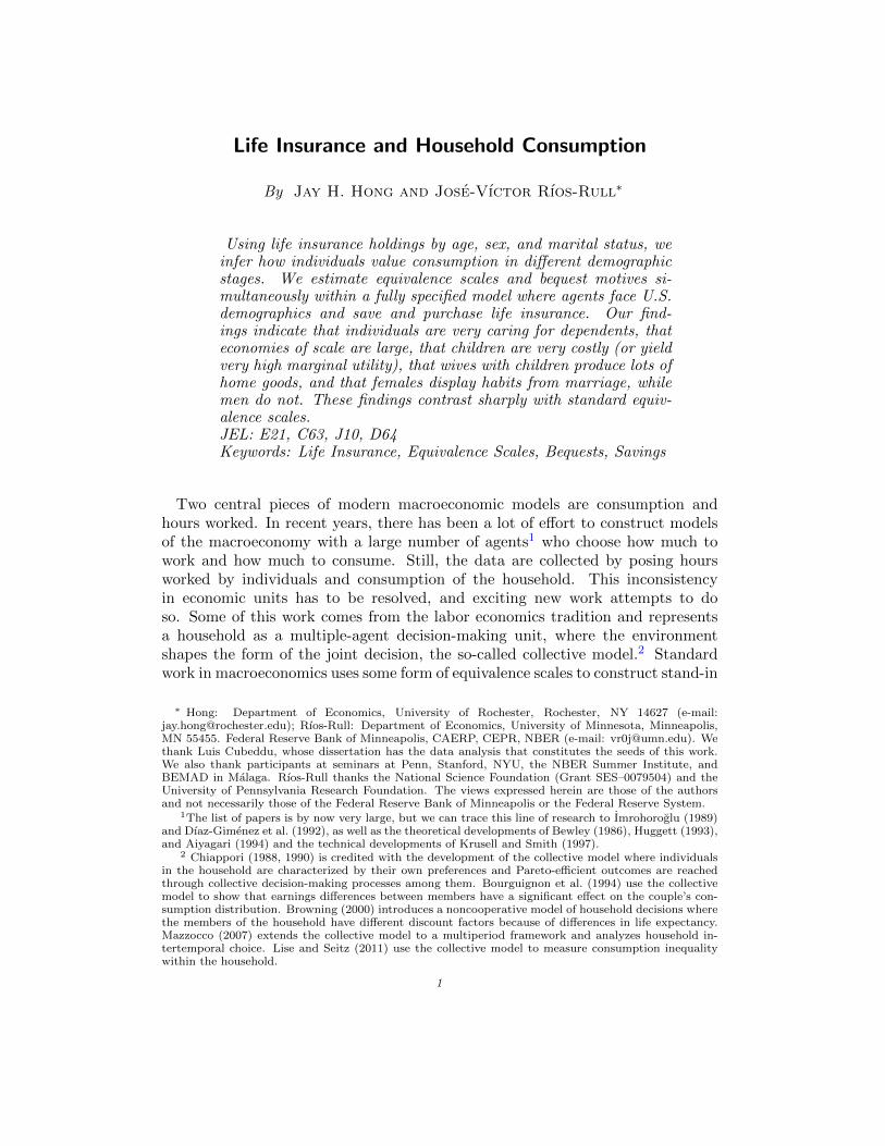
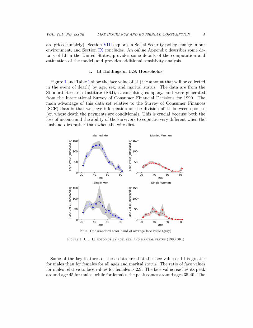
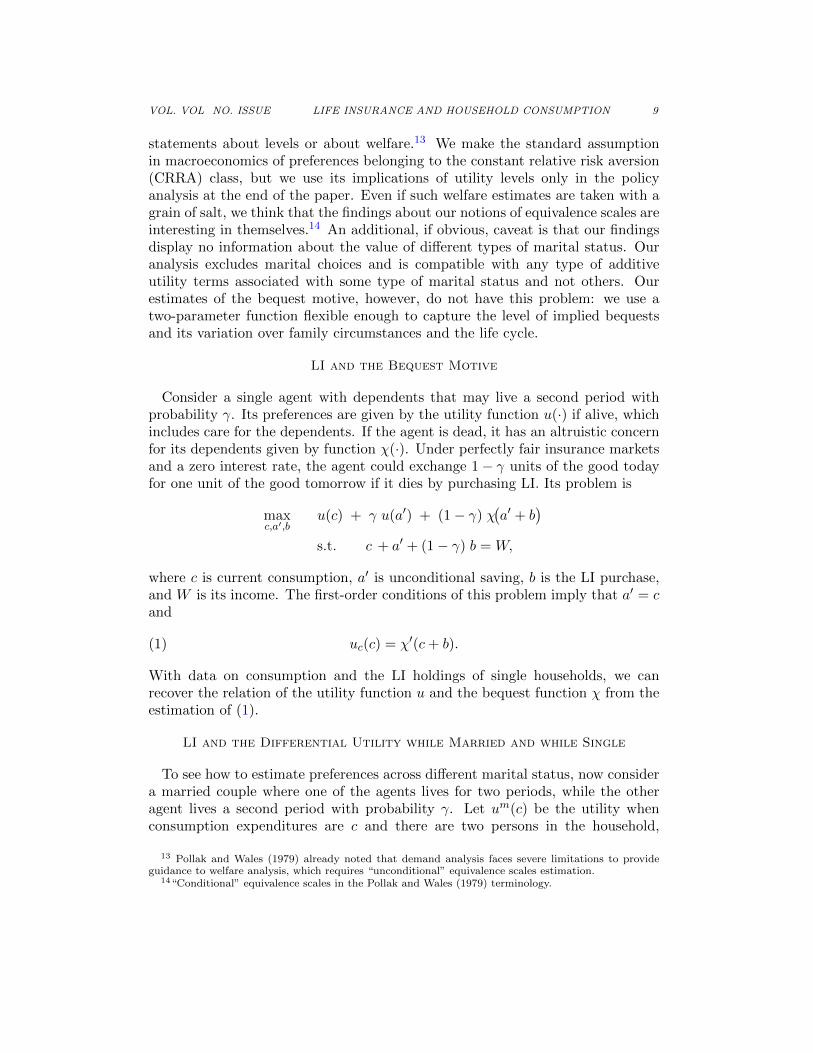
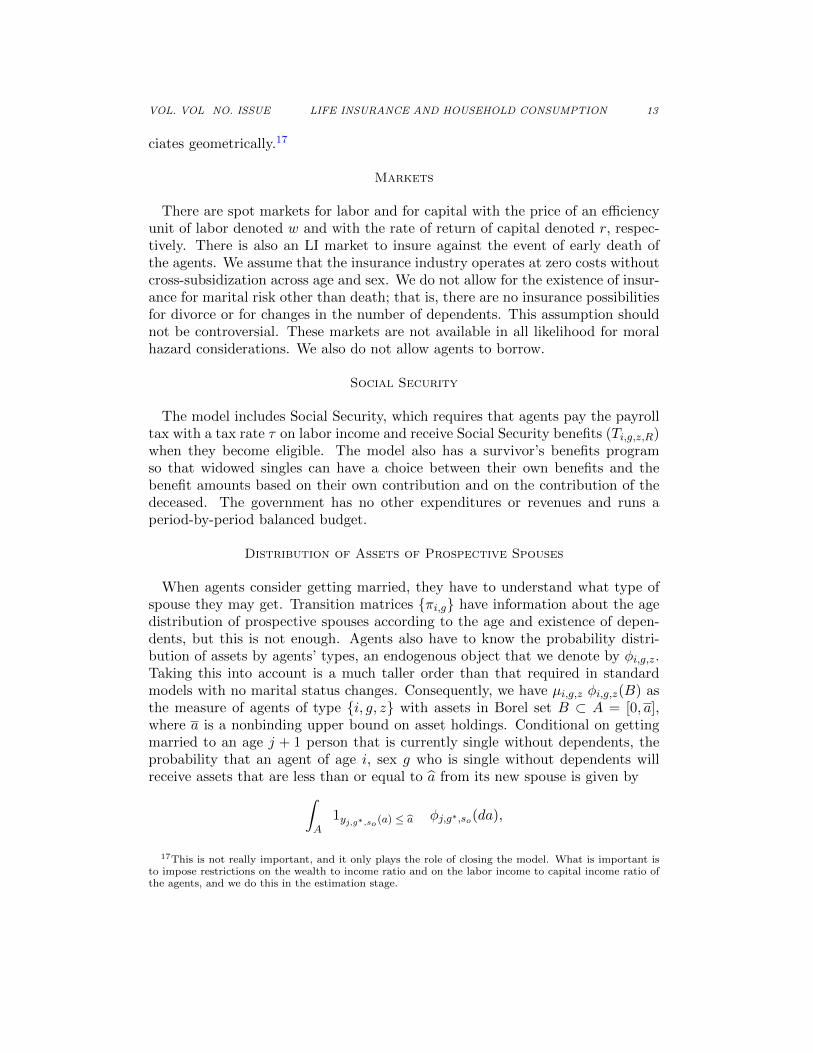
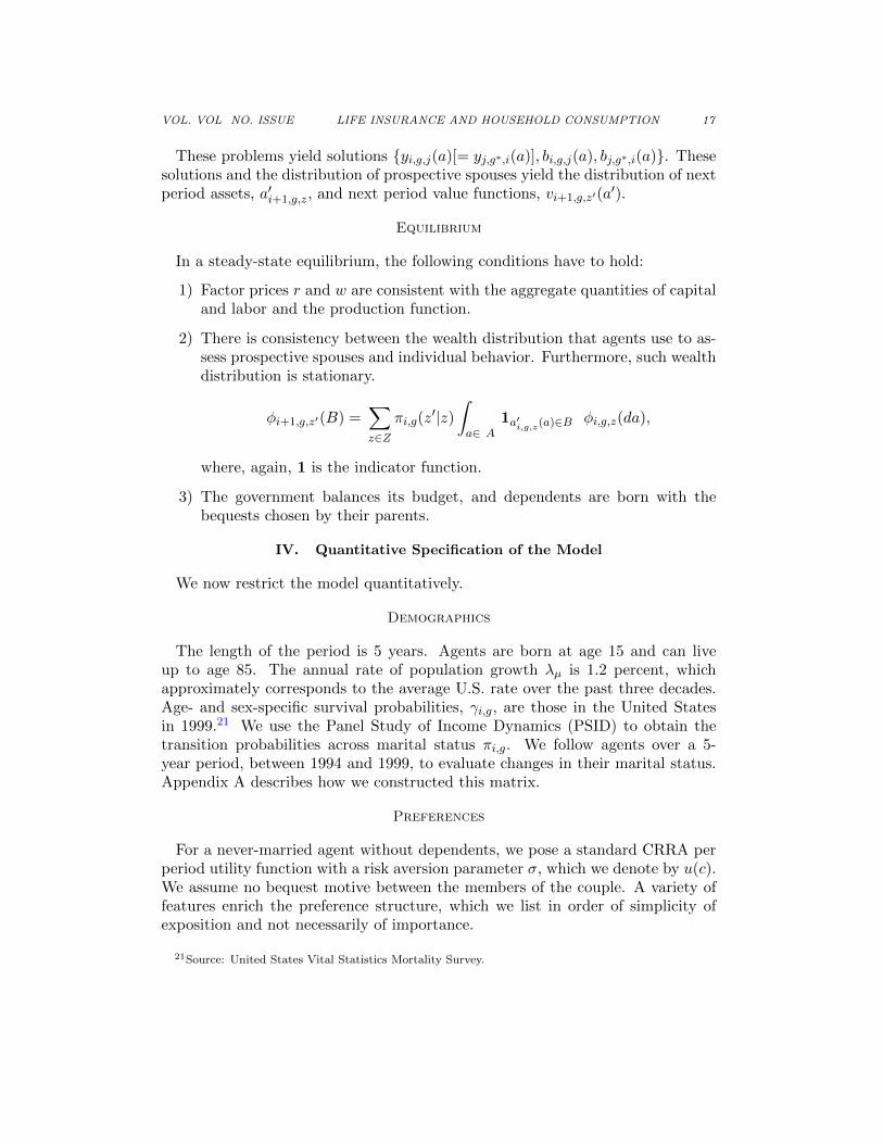
Figure 1 and Table 1 show the face value of LI (the amount that will be collectedin the event of death) by age, sex, and marital status. The data are from theStanford Research Institute (SRI), a consulting company, and were generatedfrom the International Survey of Consumer Financial Decisions for 1990. Themain advantage of this data set relative to the Survey of Consumer Finances(SCF) data is that we have information on the division of LI between spouses(on whose death the payments are conditional). This is crucial because both theloss of income and the ability of the survivors to cope are very different when thehusband dies rather than when the wife dies.
age
Face
Val
ue (T
hous
and
$)
Married Men
20 40 60 800
50
100
150
age
Face
Val
ue (T
hous
and
$)
Married Women
20 40 60 800
50
100
150
age
Face
Val
ue (T
hous
and
$)
Single Men
20 40 60 800
50
100
150
age
Face
Val
ue (T
hous
and
$)
Single Women
20 40 60 800
50
100
150
Note: One standard error band of average face value (gray)
Figure 1. U.S. LI holdings by age, sex, and marital status (1990 SRI)
Some of the key features of these data are that the face value of LI is greaterfor males than for females for all ages and marital status. The ratio of face valuesfor males relative to face values for females is 2.9. The face value reaches its peakaround age 45 for males, while for females the peak comes around ages 35-40. The
6 THE AMERICAN ECONOMIC REVIEW MONTH YEAR
face value of LI for married males (females) is on average 1.6 (1.7) times greaterthan that of single head of household males (females). For all ages, a greaterpercentage of men (76.3 percent) own LI than women (62.9 percent). Ownershipis less common for younger and older age groups than for middle-aged people.Married men and women are more likely to own LI than single men and women.The percentage of men owning LI is 77.4 percent, 75.1 percent, and 69.9 percentfor married men, single men with dependents, and single men without dependents,respectively. The percentage of women owning LI is 65.7 percent, 58.4 percent,and 55.4 percent for married women, single women with dependents, and singlewomen without dependents, respectively. We use these profiles to learn abouthow preferences depend on family structure.
Table 1—LI Statistics from SRI (1990)
Face Value (U.S. dollars) Participation (Percent)
Men Women Men Women
All 80,374 28,110 76.3 62.9
Married 85,350 32,197 77.4 65.7Single 54,930 18,718 71.1 56.5
Single /w dep 65,826 26,527 75.1 58.4
Single w/o dep 51,728 13,691 69.9 55.4
A. Data Issues about LI
We now turn to address some concerns regarding LI: the type of LI products weare referring to, and the extent to which LI is voluntarily held and fairly priced.
Term Insurance versus Whole LI
There are many types of LI products, but they can be divided into two maincategories: term insurance and whole LI. Term insurance protects a policyholder’slife only until its expiration date, after which it expires. Renewal of the policytypically involves an increase in the premium because the policyholder’s mortalityincreases with age.8 Whole LI doesn’t have an expiration date. When signingthe contract, the insurance company and the policyholders agree to set a facevalue (amount of money benefit in case of death) and a premium (monthly pay-ment). The annual premium remains constant throughout the life of the policy.Therefore, the premium charged in earlier years is higher than the actual cost ofprotection. This excess amount is reserved as the policy’s cash value. When a
8Even the LI contracts labeled as term insurance may have some front loading. Hendel and Lizzeri(2003) compared annually renewable term insurance with level term contracts that offer a premiumincrease only every few years and found that the latter have some front loading compared with annuallyrenewable policies.
VOL. VOL NO. ISSUE LIFE INSURANCE AND HOUSEHOLD CONSUMPTION 7
policyholder decides to surrender the policy, she receives the cash value at thetime of surrender. There are tax considerations to this type of insurance, sinceit can be used to reduce the tax bill. Since whole LI offers a combination ofinsurance and savings, we subtract the saving component from the face value toobtain the pure insurance amount.
On the Optimality of LI Holdings
Some of the LI held by people is obtained through employment or membershipin organizations (group insurance), and some is obtained directly from an LIcompany. Provision by the employer may imply that the amount of insurancecovered by group policies is not the result of policyholders’ optimal choices.9
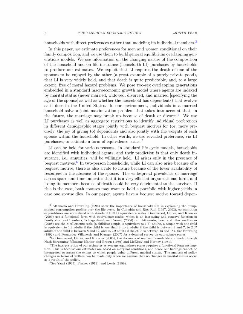
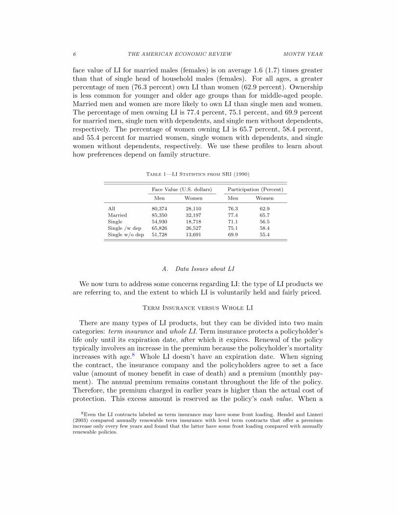
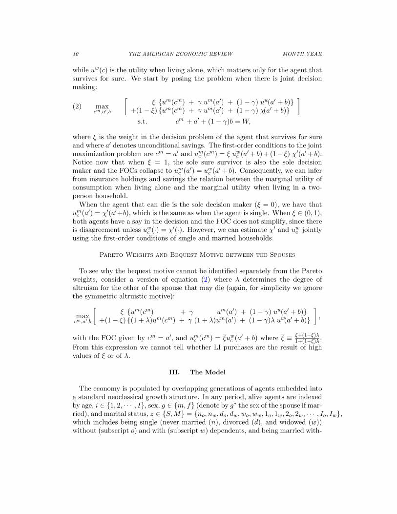
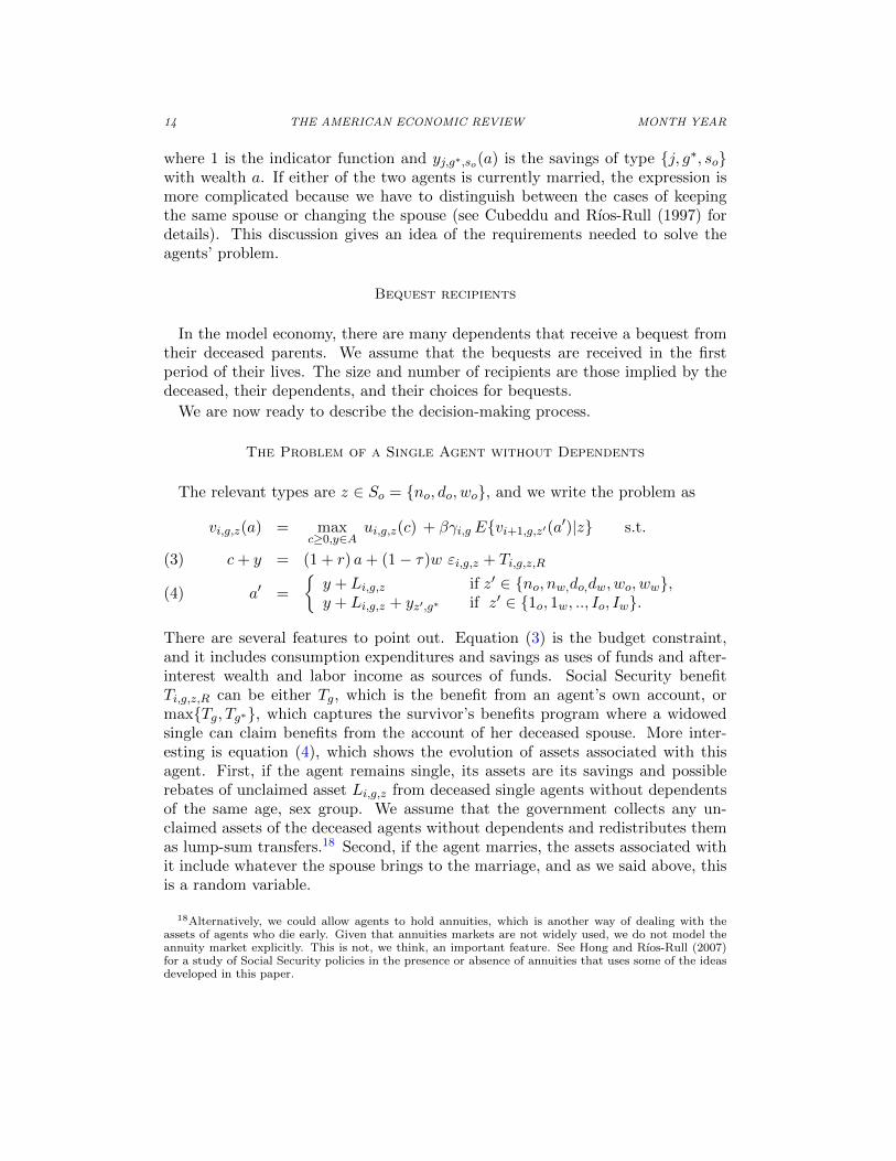
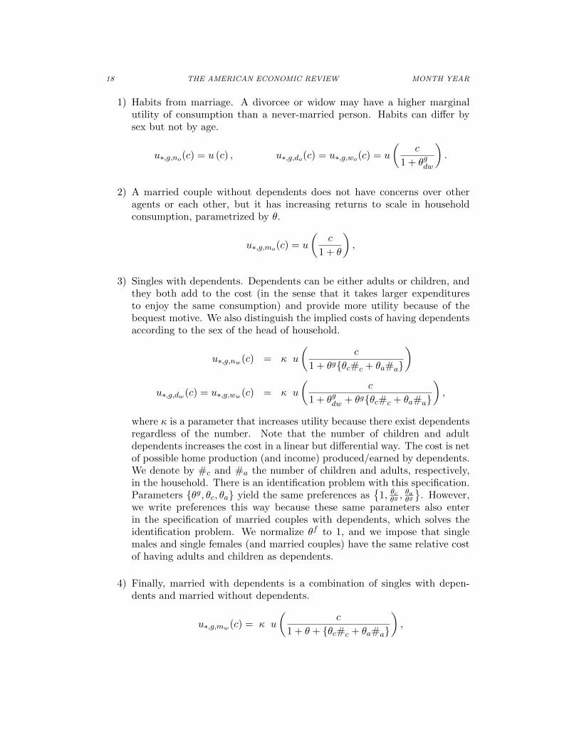
Fortunately, we can explore whether this is the case in detail because the SRIdata provide separate information on both types of policies. Among those thathold some insurance, 73 percent of men and 71 percent of women hold someindividual insurance. Clearly, for those people group insurance was not sufficient,so they hold additional insurance. In addition, individual LI is about 50 percentlarger than group LI.10 We therefore consider all holdings by people who holdboth types of insurance as voluntary and optimally chosen. Even when we imposethe very restrictive criterion that the insurance held by people who have grouppolicies only is all involuntary,11 we obtain that 84 percent of the total face valueis considered voluntary for men, 80 percent for women, and less for single women(especially for single women without dependents).12 Figure 2 shows how thisconservative measure of voluntary insurance compares with the insurance measureused as the benchmark. Tables D-5 and D-6 in the Appendix show the measureof voluntary insurance across different employment status (full-time, part-time,and non-employed). The differences across employment status are quite small. Ifemployees are given too much insurance which they don’t want, we should haveseen very low conservative measures of voluntary insurance for full-time employed,but these numbers are not very different across employment status.
Singles without dependents also hold LI. Note, however, that we use the re-ported number of household members to determine the existence of dependents,which is the right measure to relate consumption expenditures and consumptionenjoyment, but not perhaps to determine the existence of a bequest motive. Sin-gles who do not live with dependents may still have relatives outside of theirhousehold to whom they want to leave bequests in case of their death. We dis-cuss the LI holdings of singles without dependents in Section VII. Consequently,we think that to a first approximation, the consideration of insurance purchasesas voluntary is appropriate.
9In fact, this may be what accounts for the fact that up to 70 percent of single males withoutdependents own LI.
10 Tables D-1 and D-2 in the Appendix show, respectively, the participation rate and the face valueof each type of insurance policy.
11People may have actually wanted some, if not all, of the insurance provided by the organization.12Table D-3 for males and Table D-4 for females in the Appendix provide the details.
8 THE AMERICAN ECONOMIC REVIEW MONTH YEAR
20 40 60 800
50
100
150
age
Face
Val
ue (T
hous
and
$)
Married Men
TotalVoluntary
20 40 60 800
50
100
150
age
Face
Val
ue (T
hous
and
$)
Married Women
TotalVoluntary
20 40 60 800
50
100
150
age
Face
Val
ue (T
hous
and
$)
Single Men
TotalVoluntary
20 40 60 800
50
100
150
ageFa
ce V
alue
(Tho
usan
d $)
Single Women
TotalVoluntary
Figure 2. Voluntary measure of LI by age, sex, and marital status (1990 SRI)
Pricing
Our data do not have details on pricing. As noted, a majority of insuranceis purchased by people with some individual insurance. Individual insuranceis clearly not subsidized and is a marginal purchase, so we do not think thatsubsidized group insurance distorts people’s choices. Moreover, 20 percent of menand 18 percent of women hold group insurance but no individual insurance, sowe do not think that there is bias because of differential labor force participationamong the sexes. In most of our analysis, we assume that the price of LI isactuarially fair. We discuss pricing behavior associated with “load factors” in theLI industry in Section VII.
II. Retrieving Information from LI Holdings
In this section we briefly describe how we use LI holdings to make inferencesabout preferences about the bequest motive for dependents and about equivalencescales or how consumption expenditures translate into utilities across differenttypes of marital status. We also discuss the identification problem at the rootof the assumption of no bequest motive for spouses. First, a caveat: agents’decisions in this model are based on marginal considerations, and estimates basedon average allocations require a functional form assumption in order to make
VOL. VOL NO. ISSUE LIFE INSURANCE AND HOUSEHOLD CONSUMPTION 9
statements about levels or about welfare.13 We make the standard assumptionin macroeconomics of preferences belonging to the constant relative risk aversion(CRRA) class, but we use its implications of utility levels only in the policyanalysis at the end of the paper. Even if such welfare estimates are taken with agrain of salt, we think that the findings about our notions of equivalence scales areinteresting in themselves.14 An additional, if obvious, caveat is that our findingsdisplay no information about the value of different types of marital status. Ouranalysis excludes marital choices and is compatible with any type of additiveutility terms associated with some type of marital status and not others. Ourestimates of the bequest motive, however, do not have this problem: we use atwo-parameter function flexible enough to capture the level of implied bequestsand its variation over family circumstances and the life cycle.
LI and the Bequest Motive
Consider a single agent with dependents that may live a second period withprobability γ. Its preferences are given by the utility function u(·) if alive, whichincludes care for the dependents. If the agent is dead, it has an altruistic concernfor its dependents given by function χ(·). Under perfectly fair insurance marketsand a zero interest rate, the agent could exchange 1− γ units of the good todayfor one unit of the good tomorrow if it dies by purchasing LI. Its problem is
maxc,a′,b
u(c) + γ u(a′) + (1− γ) χ(a′ + b
)s.t. c + a′ + (1− γ) b = W,
where c is current consumption, a′ is unconditional saving, b is the LI purchase,and W is its income. The first-order conditions of this problem imply that a′ = cand
(1) uc(c) = χ′(c+ b).
With data on consumption and the LI holdings of single households, we canrecover the relation of the utility function u and the bequest function χ from theestimation of (1).
LI and the Differential Utility while Married and while Single
To see how to estimate preferences across different marital status, now considera married couple where one of the agents lives for two periods, while the otheragent lives a second period with probability γ. Let um(c) be the utility whenconsumption expenditures are c and there are two persons in the household,
13 Pollak and Wales (1979) already noted that demand analysis faces severe limitations to provideguidance to welfare analysis, which requires “unconditional” equivalence scales estimation.
14“Conditional” equivalence scales in the Pollak and Wales (1979) terminology.
10 THE AMERICAN ECONOMIC REVIEW MONTH YEAR
while uw(c) is the utility when living alone, which matters only for the agent thatsurvives for sure. We start by posing the problem when there is joint decisionmaking:
maxcm,a′,b
[ξ um(cm) + γ um(a′) + (1− γ) uw(a′ + b)
+(1− ξ) um(cm) + γ um(a′) + (1− γ) χ(a′ + b)
](2)
s.t. cm + a′ + (1− γ)b = W,
where ξ is the weight in the decision problem of the agent that survives for sureand where a′ denotes unconditional savings. The first-order conditions to the jointmaximization problem are cm = a′ and umc (cm) = ξ uwc (a′+ b) + (1− ξ) χ′(a′+ b).Notice now that when ξ = 1, the sole sure survivor is also the sole decisionmaker and the FOCs collapse to umc (a′) = uwc (a′+ b). Consequently, we can inferfrom insurance holdings and savings the relation between the marginal utility ofconsumption when living alone and the marginal utility when living in a two-person household.
When the agent that can die is the sole decision maker (ξ = 0), we have thatumc (a′) = χ′(a′+b), which is the same as when the agent is single. When ξ ∈ (0, 1),both agents have a say in the decision and the FOC does not simplify, since thereis disagreement unless uwc (·) = χ′(·). However, we can estimate χ′ and uwc jointlyusing the first-order conditions of single and married households.
Pareto Weights and Bequest Motive between the Spouses
To see why the bequest motive cannot be identified separately from the Paretoweights, consider a version of equation (2) where λ determines the degree ofaltruism for the other of the spouse that may die (again, for simplicity we ignorethe symmetric altruistic motive):
maxcm,a′,b
[ξ um(cm) + γ um(a′) + (1− γ) uw(a′ + b)
+(1− ξ) (1 + λ)um(cm) + γ (1 + λ)um(a′) + (1− γ)λ uw(a′ + b)
],
with the FOC given by cm = a′, and umc (cm) = ξuwc (a′ + b) where ξ ≡ ξ+(1−ξ)λ1+(1−ξ)λ .
From this expression we cannot tell whether LI purchases are the result of highvalues of ξ or of λ.
III. The Model
The economy is populated by overlapping generations of agents embedded intoa standard neoclassical growth structure. In any period, alive agents are indexedby age, i ∈ 1, 2, · · · , I, sex, g ∈ m, f (denote by g∗ the sex of the spouse if mar-ried), and marital status, z ∈ S,M = no, nw, do, dw, wo, ww, 1o, 1w, 2o, 2w, · · · , Io, Iw,which includes being single (never married (n), divorced (d), and widowed (w))without (subscript o) and with (subscript w) dependents, and being married with-
VOL. VOL NO. ISSUE LIFE INSURANCE AND HOUSEHOLD CONSUMPTION 11
out and with dependents where the index denotes the age of the spouse. Agentsare also indexed by the assets of the household to which the agent belongs a ∈ A.
While agents that survive age deterministically, one period at a time, and theynever change sex, their marital status evolves exogenously through marriage, di-vorce, widowhood, and the acquisition of dependents following a Markov processwith transition πi,g. If we denote next period’s values with primes, we havei′ = i + 1, g′ = g, and the probability of an agent of type i, g, z today movingto state z′ is πi,g(z
′|z).15
Demographics
Agents live up to a maximum of I periods and face mortality risk. Survivalprobabilities depend only on age and sex. The probability of surviving betweenage i and age i+1 for an agent of gender g is γi,g, and the unconditional probability
of being alive at age i can be written as γig = Πi−1j=1γj,g.
16 Population grows
at an exogenous rate λµ. We use µi,g,z to denote the measure of type i, g, zindividuals. Therefore, the measure of the different types satisfies
µi+1,g,z′ =∑z
γi,gπi,g(z
′|z)(1 + λµ)
µi,g,z.
An important additional restriction on the matrices πi,g has to be satisfiedfor internal consistency: the measure of age i males married to age j femalesequals the measure of age j females married to age i males, µi,m,jo = µj,f,io andµi,m,jw = µj,f,iw .
Preferences
We index preferences over per period household consumption expenditures byage, sex, and marital status ui,g,z(c). With respect to the joy of giving, weassume that upon death, a single agent with dependents gets utility from leavingits dependents with a certain amount of resources χ(·). A married agent withdependents that dies gets expected utility from the consumption of the dependentswhile they stay in the household of her spouse. Upon the death of the spouse,the bequest motive toward dependents becomes operational again. We assumethat there is no bequest motive between the spouses. The reason is that there isno known identification strategy to separately measure a bequest motive betweenthe spouses and the relative weight in the decision-making process.
If we denote with vi,g,z(a) the value function of a single agent, and if we (tem-porarily) ignore the choice problem and the budget constraints, in the case where
15Note that we abstract from assortative matching. Extending the model to account for this type ofsorting would require indexing agents by education, which would dramatically increase the computationaldemands of the problem. We leave this process for future work.
16Here we abstract from differential mortality based on marital status.
12 THE AMERICAN ECONOMIC REVIEW MONTH YEAR
the agent has dependents we have
vi,g,z(a) = ui,g,z(c) + β γi,g Evi+1,g,z′(a′)|z+ β (1− γi,g) χ(a′),
while if the agent does not have dependents, the last term is absent.
The case of a married household is slightly more complicated because of theadditional term that represents the utility obtained from the dependents’ con-sumption while under the care of the former spouse. Again, using vi,g,j(a) todenote the value function of an age i agent of sex g married to a sex g∗ of age jand ignoring decision-making and budget constraints, we have
vi,g,j(a) = ui,g,j(c) + β γi,g Evi+1,g,z′(a′)|z +
β (1− γi,g) (1− γj,g∗) χ(a′) + β (1− γi,g) γj,g∗ EΩj+1,g∗,z′g∗
(a′g∗),
where the first two terms on the right-hand side are standard, the third term rep-resents the utility that the agent gets from the bequest motive toward dependentsthat happens if both members of the couple die, and where the fourth term withfunction Ω represents the well-being of the dependents when the spouse survivesand they are under its supervision. Function Ωi,g,z is
Ωi,g,z(a) = ui,g,z(c) + β γi,g EΩi+1,g,z′(a′)|z+ β (1− γi,g) χ(a′),
where ui,g,z(c) is the utility obtained from dependents (not the spouse) under thecare of a former spouse that now has type i, g, z and expenditures c. Noticethat we assume that an agent expects to get utility even if dead through i) thestream of utilities that are enjoyed by its dependents (but not the spouse) until thespouse dies given by u, and ii) the bequest the former spouse might leave to itsdependents upon death. This aspect of the model captures the fact that the well-being of the dependents is now under the control of the surviving spouse, whosedecision on consumption/saving would be different from that of the deceasedindividual. Note also that function Ω does not involve decision making. It does,however, involve the forecasting of what the former spouse will do, which impliesthat the FOC has the features of a generalized Euler equation (see Klein, Krusell,and Rıos-Rull (2008)).
Endowments and Technology
Every period, agents are endowed with εi,g,z units of efficient labor. Note thatin addition to age and sex, we are indexing this endowment by marital status,and this term includes labor earnings in addition to alimony and child support.All idiosyncratic uncertainty is thus related to marital status and survival.
There is an aggregate neoclassical production function that uses aggregate cap-ital, the only form of wealth holding, and efficient units of labor. Capital depre-
VOL. VOL NO. ISSUE LIFE INSURANCE AND HOUSEHOLD CONSUMPTION 13
ciates geometrically.17
Markets
There are spot markets for labor and for capital with the price of an efficiencyunit of labor denoted w and with the rate of return of capital denoted r, respec-tively. There is also an LI market to insure against the event of early death ofthe agents. We assume that the insurance industry operates at zero costs withoutcross-subsidization across age and sex. We do not allow for the existence of insur-ance for marital risk other than death; that is, there are no insurance possibilitiesfor divorce or for changes in the number of dependents. This assumption shouldnot be controversial. These markets are not available in all likelihood for moralhazard considerations. We also do not allow agents to borrow.
Social Security
The model includes Social Security, which requires that agents pay the payrolltax with a tax rate τ on labor income and receive Social Security benefits (Ti,g,z,R)when they become eligible. The model also has a survivor’s benefits programso that widowed singles can have a choice between their own benefits and thebenefit amounts based on their own contribution and on the contribution of thedeceased. The government has no other expenditures or revenues and runs aperiod-by-period balanced budget.
Distribution of Assets of Prospective Spouses
When agents consider getting married, they have to understand what type ofspouse they may get. Transition matrices πi,g have information about the agedistribution of prospective spouses according to the age and existence of depen-dents, but this is not enough. Agents also have to know the probability distri-bution of assets by agents’ types, an endogenous object that we denote by φi,g,z.Taking this into account is a much taller order than that required in standardmodels with no marital status changes. Consequently, we have µi,g,z φi,g,z(B) asthe measure of agents of type i, g, z with assets in Borel set B ⊂ A = [0, a],where a is a nonbinding upper bound on asset holdings. Conditional on gettingmarried to an age j + 1 person that is currently single without dependents, theprobability that an agent of age i, sex g who is single without dependents willreceive assets that are less than or equal to a from its new spouse is given by∫
A1yj,g∗,so (a) ≤ a φj,g∗,so(da),
17This is not really important, and it only plays the role of closing the model. What is important isto impose restrictions on the wealth to income ratio and on the labor income to capital income ratio ofthe agents, and we do this in the estimation stage.
14 THE AMERICAN ECONOMIC REVIEW MONTH YEAR
where 1 is the indicator function and yj,g∗,so(a) is the savings of type j, g∗, sowith wealth a. If either of the two agents is currently married, the expression ismore complicated because we have to distinguish between the cases of keepingthe same spouse or changing the spouse (see Cubeddu and Rıos-Rull (1997) fordetails). This discussion gives an idea of the requirements needed to solve theagents’ problem.
Bequest recipients
In the model economy, there are many dependents that receive a bequest fromtheir deceased parents. We assume that the bequests are received in the firstperiod of their lives. The size and number of recipients are those implied by thedeceased, their dependents, and their choices for bequests.
We are now ready to describe the decision-making process.
The Problem of a Single Agent without Dependents
The relevant types are z ∈ So = no, do, wo, and we write the problem as
vi,g,z(a) = maxc≥0,y∈A
ui,g,z(c) + βγi,g Evi+1,g,z′(a′)|z s.t.
c+ y = (1 + r) a+ (1− τ)w εi,g,z + Ti,g,z,R(3)
a′ =
y + Li,g,z if z′ ∈ no, nw,do,dw, wo, ww,y + Li,g,z + yz′,g∗ if z′ ∈ 1o, 1w, .., Io, Iw.
(4)
There are several features to point out. Equation (3) is the budget constraint,and it includes consumption expenditures and savings as uses of funds and after-interest wealth and labor income as sources of funds. Social Security benefitTi,g,z,R can be either Tg, which is the benefit from an agent’s own account, ormaxTg, Tg∗, which captures the survivor’s benefits program where a widowedsingle can claim benefits from the account of her deceased spouse. More inter-esting is equation (4), which shows the evolution of assets associated with thisagent. First, if the agent remains single, its assets are its savings and possiblerebates of unclaimed asset Li,g,z from deceased single agents without dependentsof the same age, sex group. We assume that the government collects any un-claimed assets of the deceased agents without dependents and redistributes themas lump-sum transfers.18 Second, if the agent marries, the assets associated withit include whatever the spouse brings to the marriage, and as we said above, thisis a random variable.
18Alternatively, we could allow agents to hold annuities, which is another way of dealing with theassets of agents who die early. Given that annuities markets are not widely used, we do not model theannuity market explicitly. This is not, we think, an important feature. See Hong and Rıos-Rull (2007)for a study of Social Security policies in the presence or absence of annuities that uses some of the ideasdeveloped in this paper.
VOL. VOL NO. ISSUE LIFE INSURANCE AND HOUSEHOLD CONSUMPTION 15
The Problem of a Single Agent with Dependents
The relevant types are z ∈ Sw = nw, dw, ww, and we write the problem as
vi,g,z(a) = maxc≥0,b≥0,y∈A
ui,g,z(c) + βγi,g Evi+1,g,z′(a′)|z+ β (1− γi,g) χ(y + b)
s.t. c+ y + qi,gb = (1 + r) a+ (1− τ)w εi,g,z + Ti,g,z,R
a′ =
y if z′ ∈ no, nw,do,dw, wo, ww,y + yz′,g∗ if z′ ∈ 1o, 1w, .., Io, Iw.
Note that here we decompose savings into uncontingent savings and LI that paysonly in case of death and that goes straight to the dependents.19 The face valueof the LI paid is b, and the total premium is qi,gb, where the premium per dollaris qi,g = (1− γi,g) when the price of LI is actuarially fair.
The Problem of a Married Couple without Dependents
The household itself does not have preferences, yet it makes decisions. Note thatthere is no agreement between the two spouses, since they have different outlooks(in case of divorce, they have different future earnings, and their subsequent familytype and life horizons are different). We make the following assumptions aboutthe internal workings of a family:
1) Spouses are constrained to enjoy equal marginal utility from current con-sumption. Sufficient conditions for this assumption are that all consumptionis private, that both spouses are constrained to have equal consumption, andthat they have equal utility functions.20
2) The household solves a joint maximization problem with weights: ξi,m,j =1−ξj,f,i. Given that both spouses have equal marginal utility out of currentconsumption, the role of different weights only affects how the first-ordercondition of the maximization problem treats consumption in future statesthat are not shared because of either early death or divorce.
3) Upon divorce, assets are divided, a fraction, ψi,g,j , goes to the age i sexg agent and a fraction, ψj,g∗,i, goes to the spouse. The sum of these twofractions may be less than 1 because of divorce costs.
4) Upon the death of a spouse, the remaining beneficiary receives a deathbenefit from the spouse’s LI if the deceased held any LI.
19Allowing agents with dependents to choose annuities does not change the allocation chosen as longas they have a strong bequest motive. In fact, LI is the opposite of an annuity.
20The constraint can also be implemented with all consumption being public or with some publicconsumption and some private, equally shared consumption, or with private consumption in fixed pro-portions between the two spouses and a certain relation between the utility functions of each. Theseconstraints are independent of the utility weights.
16 THE AMERICAN ECONOMIC REVIEW MONTH YEAR
With these assumptions, the problem solved by the household is
maxc≥0,bg≥0,bg∗≥0,,y∈A
ui,g,j(c) + ξi,g,j β γi,g Evi+1,g,z′g(a′g)|j+
ξj,g∗,i β γj,g∗ Evj+1,g∗,z′g∗
(a′g∗)|i
(5) s.t. c+ y+ qi,gbg + qj,g∗bg∗ = (1 + r) a+ (1− τ)w(εi,g,j + εj,g∗,i) +Ti,g,j,R
a′g = a′g∗ = y + Li,g,j , if remain married z′ = j + 1a′g = ψi,g,j (y + Li,g,j),a′g∗ = ψj,g∗,i (y + Li,g,j),
if divorced and no remarriage, z′ ∈ S
a′g = ψi,g,j (y + Li,g,j) + yz′g ,g∗ ,
a′g∗ = ψj,g∗,i (y + Li,g,j) + yz′g∗ ,g
,if divorced and remarriage, z′ ∈M
a′g = y + Li,g,j + bg∗ ,a′g∗ = y + Li,g,j + bg,
if widowed and no remarriage, z′ ∈ S
a′g = y + Li,g,j + bg∗ + yz′g ,g∗ ,
a′g∗ = y + Li,g,j + bg + yz′g∗ ,g
.if widowed and remarriage, z′ ∈M,
(6)
where Li,g,j is the lump-sum rebate of the unclaimed assets in case of joint deathof couples without dependents. Note that the household may purchase differentamounts of LI, depending on who dies. Equation (6) describes the evolution ofassets for both household members under different scenarios of future maritalstatus.
The problem of a Married Couple with Dependents
The problem of a married couple with dependents is slightly more complicated,since it involves altruistic concerns. The main change is the objective function:
maxc≥0,bg≥0,bg∗≥0,y∈A
ui,g,j(c) + β (1− γi,g) (1− γj,g∗) χ(y + bg + bg∗) +
ξi,g,j βγi,g Evi+1,g,z′g(a
′g)|j + (1− γi,g) γj,g∗ Ωj+1,g∗,z′ (y + bg)
+
ξj,g∗,i βγj,g∗ Evj+1,g∗,z′
g∗(a′g∗)|i+ (1− γj,g∗) γi,g Ωi+1,g,z′
(y + b∗g
).
The budget constraint is as in equation (5). In this case if both spouses die, theirassets go to their dependents. The law of motion for assets becomes equation (6)with Li,g,j = 0. Note also how the weights do not enter either the current utilityor the utility obtained via the bequest motive if both spouses die, since bothspouses agree over these terms. Recall that function Ω does not involve decisions,but it involves forecasting the former spouse’s future decisions.
VOL. VOL NO. ISSUE LIFE INSURANCE AND HOUSEHOLD CONSUMPTION 17
These problems yield solutions yi,g,j(a)[= yj,g∗,i(a)], bi,g,j(a), bj,g∗,i(a). Thesesolutions and the distribution of prospective spouses yield the distribution of nextperiod assets, a′i+1,g,z, and next period value functions, vi+1,g,z′(a
′).
Equilibrium
In a steady-state equilibrium, the following conditions have to hold:
1) Factor prices r and w are consistent with the aggregate quantities of capitaland labor and the production function.
2) There is consistency between the wealth distribution that agents use to as-sess prospective spouses and individual behavior. Furthermore, such wealthdistribution is stationary.
φi+1,g,z′(B) =∑z∈Z
πi,g(z′|z)
∫a∈ A
1a′i,g,z(a)∈B φi,g,z(da),
where, again, 1 is the indicator function.
3) The government balances its budget, and dependents are born with thebequests chosen by their parents.
IV. Quantitative Specification of the Model
We now restrict the model quantitatively.
Demographics
The length of the period is 5 years. Agents are born at age 15 and can liveup to age 85. The annual rate of population growth λµ is 1.2 percent, whichapproximately corresponds to the average U.S. rate over the past three decades.Age- and sex-specific survival probabilities, γi,g, are those in the United Statesin 1999.21 We use the Panel Study of Income Dynamics (PSID) to obtain thetransition probabilities across marital status πi,g. We follow agents over a 5-year period, between 1994 and 1999, to evaluate changes in their marital status.Appendix A describes how we constructed this matrix.
Preferences
For a never-married agent without dependents, we pose a standard CRRA perperiod utility function with a risk aversion parameter σ, which we denote by u(c).We assume no bequest motive between the members of the couple. A variety offeatures enrich the preference structure, which we list in order of simplicity ofexposition and not necessarily of importance.
21Source: United States Vital Statistics Mortality Survey.
18 THE AMERICAN ECONOMIC REVIEW MONTH YEAR
1) Habits from marriage. A divorcee or widow may have a higher marginalutility of consumption than a never-married person. Habits can differ bysex but not by age.
u∗,g,no(c) = u (c) , u∗,g,do(c) = u∗,g,wo(c) = u
(c
1 + θgdw
).
2) A married couple without dependents does not have concerns over otheragents or each other, but it has increasing returns to scale in householdconsumption, parametrized by θ.
u∗,g,mo(c) = u
(c
1 + θ
),
3) Singles with dependents. Dependents can be either adults or children, andthey both add to the cost (in the sense that it takes larger expendituresto enjoy the same consumption) and provide more utility because of thebequest motive. We also distinguish the implied costs of having dependentsaccording to the sex of the head of household.
u∗,g,nw(c) = κ u
(c
1 + θgθc#c + θa#a
)
u∗,g,dw(c) = u∗,g,ww(c) = κ u
(c
1 + θgdw + θgθc#c + θa#a
),
where κ is a parameter that increases utility because there exist dependentsregardless of the number. Note that the number of children and adultdependents increases the cost in a linear but differential way. The cost is netof possible home production (and income) produced/earned by dependents.We denote by #c and #a the number of children and adults, respectively,in the household. There is an identification problem with this specification.Parameters θg, θc, θa yield the same preferences as
1, θcθg ,
θaθg
. However,
we write preferences this way because these same parameters also enterin the specification of married couples with dependents, which solves theidentification problem. We normalize θf to 1, and we impose that singlemales and single females (and married couples) have the same relative costof having adults and children as dependents.
4) Finally, married with dependents is a combination of singles with depen-dents and married without dependents.
u∗,g,mw(c) = κ u
(c
1 + θ + θc#c + θa#a
),
VOL. VOL NO. ISSUE LIFE INSURANCE AND HOUSEHOLD CONSUMPTION 19
which assumes that the costs of dependents are the same for couples andsingle women.22
We assume the utility obtained from dependents who are under the care of asurviving spouse is ui,g,z(c) = κ−1
κ ui,g,z(c). We pose the bequest function χ to
be a CRRA function, χ(x) = χax1−χb1−χb . Note that two parameters are needed to
control both the average and the derivative of the bequest intensity. In addition,we assume that the spouses may have different weights when solving their jointmaximization problem, ξm + ξf = 1. Note that this weight is constant regardlessof the age of each spouse.23
With all of this, we have 12 parameters: the discount factor β, the weightof the male in the married household maximization problem, ξm, the coefficientof risk aversion σ, and those parameters related to the multiperson household
θmdw, θfdw, θ, θ
m, θc, θa, χa, χb, κ. We restrict θmdw, θa to be 0, which means thatthere is no habit from marriage for men and adult dependents are costless. Es-timating the model with these two parameters restricted to be nonnegative only(the only values that allow for a sensible interpretation) yielded estimated val-ues of zero, so we impose this restriction. We leave these two parameters in thegeneral specification of the model for the sake of comparison with our alternativespecifications. We also set the risk aversion parameter to 3, and we estimate allother parameters.
Other Features from the Marriage
We still have to specify other features from the marriage. With respect to thepartition of assets upon divorce, we assume an equal share24 (ψ·,m,· = ψ·,f,· = 0.5).For married couples and singles with dependents, the number of dependents ineach household matters because they increase the cost of achieving each utilitylevel. We use the Current Population Survey (CPS) of 1989-1991 to get theaverage number of child and adult dependents for each age, sex, and maritalstatus (reported in Tables D-7 and D-8 of the Appendix). For married couples,we compute the average number of dependents based on the wife’s age. Singlewomen have more dependents than single men, and widows/widowers tend to havemore dependents than any other single group. The number of children peaks atage 30-35 for both sexes, while the number of adult dependents peaks at age 55-60or 60-65.
22We allowed these costs to vary, and it turned out that the estimates are very similar and the gainin accuracy quite small, so we imposed these costs to be identical as long as there is a woman in thehousehold.
23 Lundberg, Startz, and Stillman (2003) show that the relative weight shifts in favor of the wifeas couples get older when women live longer than men. This weight could also depend on the relativeincome of each member of the couple, which in our model is a function of the age of each spouse andmarital status. See also Browning and Chiappori (1998) and Mazzocco (2007).
24Unlike Cubeddu and Rıos-Rull (1997, 2003), we account explicitly for child support and alimony inour specification of earnings, which makes it unnecessary to use the asset partition as an indirect way ofmodeling transfers between former spouses.
20 THE AMERICAN ECONOMIC REVIEW MONTH YEAR
Endowments and Technology
To compute the earnings of agents, we use the CPS March files for 1989-1991reported in Table D-9 of the Appendix. Labor earnings for different years areadjusted using the 1990 GDP deflator. Labor earnings, εi,g,z, are distinguishedby age, sex, and marital status. We split the sample into 7 different maritalstatuses M,no, nw, do, dw, wo, ww.25 Single men with dependents have higherearnings than those without dependents. This pattern, however, is reversed forsingle women: those never married have the highest earnings, followed by divorcedand then widowed women. But for single men, those divorced have the highestearnings, followed by widowed and never married men.26 The earnings that weuse include alimony and child support paid and received. We collect data on thealimony and child support income of divorced women from the same CPS datareported in Table D-10 of the Appendix. We then add age-specific alimony andchild support income to the earnings of divorced women on a per capita basis.We reduce the earnings of divorced men correspondingly. Note that we cannotkeep track of those married men who pay child support from previous marriages.
We use 1991 Social Security beneficiary data to compute average benefits perhousehold.27 We break eligible households into 3 groups depending on whetherit has both a male and a female worker retired, a male worker only, or a fe-male worker only. In 1991, the average monthly benefit amounts per family were$,1068, $712, and $542, respectively. To account for the survivor benefits of SocialSecurity, we allow for a widow to collect the benefits of her deceased spouse in-stead of those of her own upon her retirement, Twf = maxTm, Tf.28 People areeligible to collect benefits starting at age 65. Aggregating these benefits requiresa Social Security tax rate τ of 11 percent.29
We also assume a Cobb-Douglas production function where the capital share is0.36. We set annual depreciation to be 8 percent.
V. Estimation
We estimate the 9 parameters, Θ = θmdw, θfdw, θ, θ
m, θc, θa, χa, χb, κ, of thebenchmark model economy jointly by matching 48 moment conditions, the aver-ages of simulated and actual age (12 groups), sex (2 groups), and marital status(2 groups) profiles of LI and imposing a model-generated wealth to earnings ratio
25This is a compromise for not having hours worked. Married men have higher earnings than singlemen, while the opposite is true for women.
26While the correlation between earnings and family composition is likely to be closely related toselection, in this paper we just want to reproduce such relation, which ends up implying that demographicsare what cause earnings. Since in this model demographics are modeled as exogenous, we think that isa reasonable assumption.
27Source: http://www.socialsecurity.gov/OACT/ProgData/famben.html.28In 1991 the average monthly survivor benefit per family for a widow is $618.66, which is in between
the amount received by a male worker only retired and a female worker only retired. This may be becauseof the higher mortality of workers with lower earnings, which our model is abstracted from.
29Throughout the paper we have assumed that defined benefits pensions are consolidated with generalhousehold savings, and consequently, only Social Security has the form of a defined benefits pension.
VOL. VOL NO. ISSUE LIFE INSURANCE AND HOUSEHOLD CONSUMPTION 21
of 3.230 using the method of simulated moments (MSM).31 We use our modelto simulate life cycle profiles, obtaining a sample of 4,000 individuals per eachage and sex from age 15 to age 85 (14 age groups) for a total of 112,000. The
estimates Θ solvemin
Θg(Θ)′ W g(Θ),
where g(Θ) = (g1(Θ), · · · , gJ(Θ))′ and gj(Θ) = mj−mj(Θ), which is the distancebetween the empirical and the simulated average face value of LI for each age–sex–marital status group (J = 48). In the benchmark model, singles withoutdependents do not hold LI. For this reason, we exclude singles without dependentswhen matching the simulated LI profile from the model to the data. We relax thisrestriction in Section VII where singles without dependents do have an operationalbequest motive. For most of the analysis, we use as weighting matrix W theidentity matrix, but we also use another one based on sampling errors, which willbe discussed in Section E of the Appendix. The variance-covariance estimator iscalculated by
ΣΘ
= (G′WG)−1G′WΩWG(G′WG)−1,
where G = ∂∂Θg|Θ=Θ
, which we compute using the numerical derivatives of g
at Θ, and Ω is the variance matrix of the empirical moments. As a measure ofthe goodness of fit of the estimation, we provide the size of the residuals of thefunction we are minimizing. We also provide the pictures of the U.S. LI holdingsdata and the model LI holdings by age, sex, and marital status.
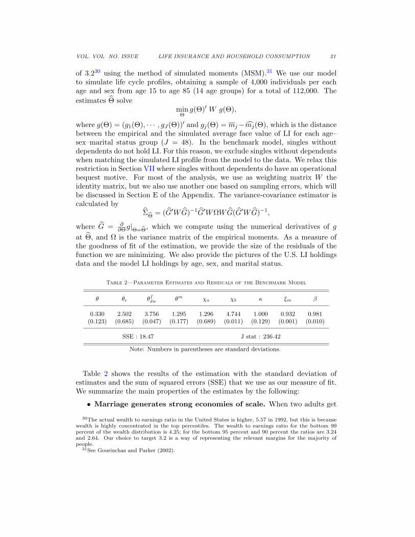
Table 2—Parameter Estimates and Residuals of the Benchmark Model
θ θc θfdw θm χa χb κ ξm β
0.330 2.502 3.756 1.295 1.296 4.744 1.000 0.932 0.981(0.123) (0.685) (0.047) (0.177) (0.689) (0.011) (0.129) (0.001) (0.010)
SSE : 18.47 J stat : 236.42
Note: Numbers in parentheses are standard deviations.
Table 2 shows the results of the estimation with the standard deviation ofestimates and the sum of squared errors (SSE) that we use as our measure of fit.We summarize the main properties of the estimates by the following:
• Marriage generates strong economies of scale. When two adults get
30The actual wealth to earnings ratio in the United States is higher, 5.57 in 1992, but this is becausewealth is highly concentrated in the top percentiles. The wealth to earnings ratio for the bottom 99percent of the wealth distribution is 4.25; for the bottom 95 percent and 90 percent the ratios are 3.24and 2.64. Our choice to target 3.2 is a way of representing the relevant margins for the majority ofpeople.
31See Gourinchas and Parker (2002).
22 THE AMERICAN ECONOMIC REVIEW MONTH YEAR
20 40 60 800
50
100
150
age
Face
Val
ue (T
hous
and
$)
Married Men
DataModel
20 40 60 800
50
100
150
age
Face
Val
ue (T
hous
and
$)
Married Women
DataModel
20 40 60 800
50
100
150
age
Face
Val
ue (T
hous
and
$)
Single Men
DataModel
20 40 60 800
50
100
150
age
Face
Val
ue (T
hous
and
$)
Single Women
DataModel
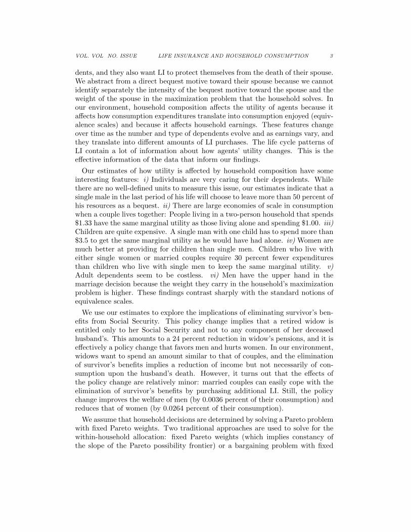
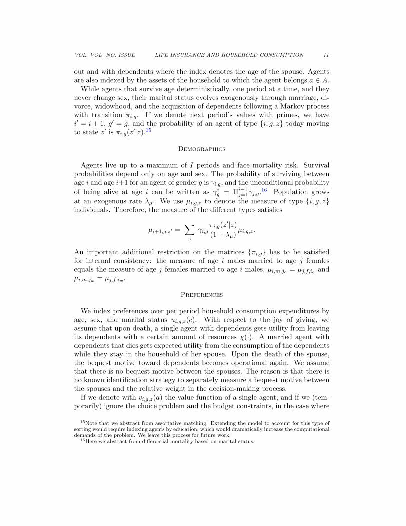
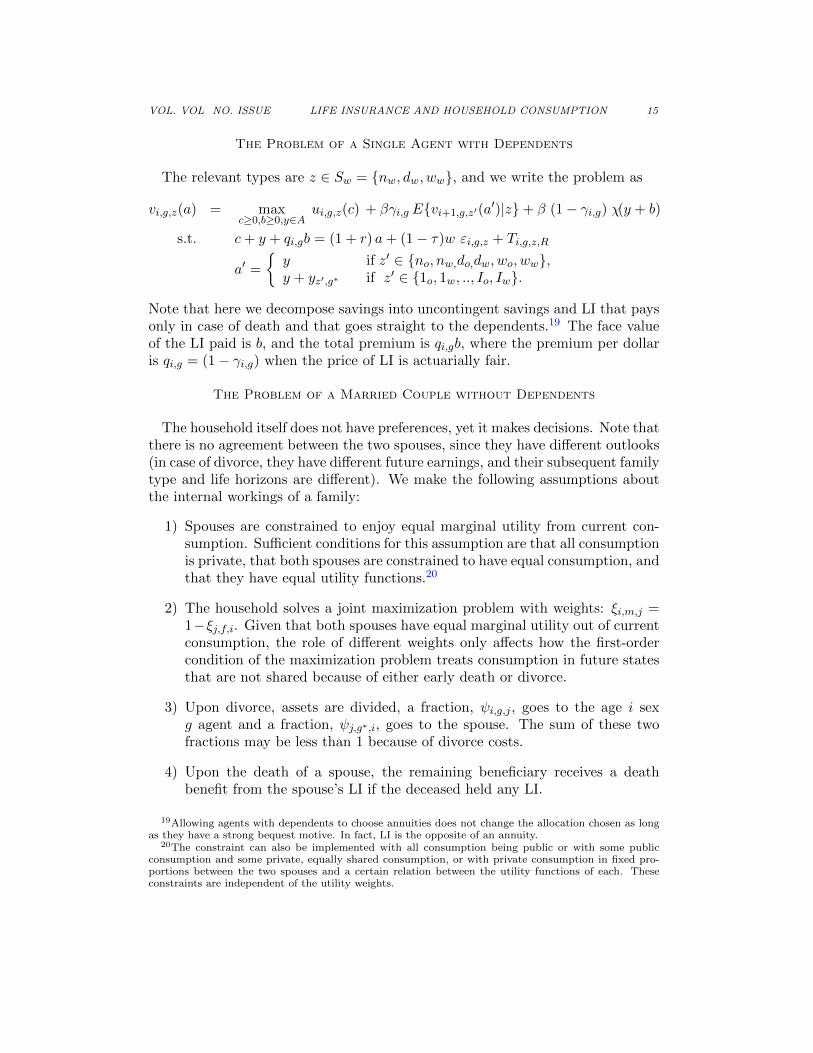
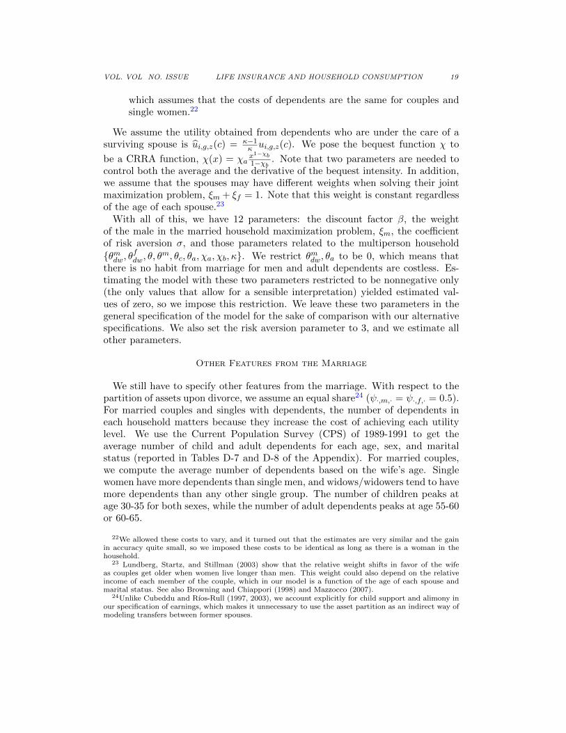
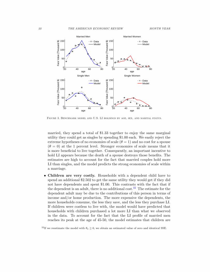
Figure 3. Benchmark model and U.S. LI holdings by age, sex, and marital status.
married, they spend a total of $1.33 together to enjoy the same marginalutility they could get as singles by spending $1.00 each. We easily reject theextreme hypotheses of no economies of scale (θ = 1) and no cost for a spouse(θ = 0) at the 1 percent level. Stronger economies of scale means that itis more beneficial to live together. Consequently, an important incentive tohold LI appears because the death of a spouse destroys those benefits. Theestimates are high to account for the fact that married couples hold moreLI than singles, and the model predicts the strong economies of scale withina marriage.
• Children are very costly. Households with a dependent child have tospend an additional $2.502 to get the same utility they would get if they didnot have dependents and spent $1.00. This contrasts with the fact that ifthe dependent is an adult, there is no additional cost.32 The estimate for thedependent adult may be due to the contributions of this person in terms ofincome and/or home production. The more expensive the dependents, themore households consume, the less they save, and the less they purchase LI.If children were costless to live with, the model would have predicted thathouseholds with children purchased a lot more LI than what we observedin the data. To account for the fact that the LI profile of married menreaches its peak at the age of 45-50, the model estimates that children are
32If we reestimate the model with θa ≥ 0, we obtain an estimated value of zero and identical SSE.
VOL. VOL NO. ISSUE LIFE INSURANCE AND HOUSEHOLD CONSUMPTION 23
costly so that young married men (who are more likely to have children inthis household) hold less LI than that of the middle-age group. Withoutthis estimate, the model would predict that the LI profile peaks too earlyin the lives of young married men. The cost of dependent children does notmatter much after age 50: there are very few children by then. Also, a lowcost of dependents implies that women’s advantage in home production isless valuable. This in turn gives less incentive to insure against the deathof a wife, which is why the model also predicts little insurance for marriedwomen. This parameter is identified essentially by the timing of the peakof married men’s insurance profiles.
• Children are less costly for females than for males. A dependentcosts a single man 30 percent more than it costs single women or marriedcouples. This indicates that females produce a lot of home goods. Withoutthis advantage of women with children dependents, the model would havepredicted too little LI for women between ages 25 and 45.
• Agents care a lot for their dependents. Our estimates imply thatthe average single man of age I with dependents consumes 45.8 cents andgives 54.2 cents as a bequest. The estimates for single women with depen-dents are 56.9 cents of consumption and 43.1 cents of bequest, ranging fromconsuming 37 cents for never married to 61.6 cents for a widow.33
• Marriage generates habits for women. The divorcee or widow is differ-ent from a never-married female. A divorced/widowed woman has to spendan additional $3.756 to enjoy the same utility of a never-married womanwho spends $1.00. This is not the case for men.34 Retired married menpurchase a lot of LI at a time when there are no dependents and when theirwives will see their future income only minimally reduced given the natureof survivor’s benefits in the United States. The estimation accounts for thisby posing a high marginal utility of consumption for widows via the habitsparameter. Note that the absence (or at least the very limited existence) ofdependents at this stage of the life cycle prevents altruistic considerationstoward those dependents to account for the high amount of LI.
• Men have a higher weight in the joint-decision problem. See Sec-tion VI.
Figure 3 shows the results of the estimation by comparing the values of LIholdings by age, sex, and marital status, both in the model and in the data. Themodel replicates all the main features of the data that we described in Section I.The only shortcoming of the model may be in the holdings of single women where
33This large variation is due to the possible presence of marriage habits.34If we reestimate the model with θmdw ≥ 0, we obtain an estimated value of zero and identical SSE.
24 THE AMERICAN ECONOMIC REVIEW MONTH YEAR
the model slightly underpredicts the LI holdings of young single women and over-predicts the LI holdings of older single women.35 Possible explanations are thatthere is a cohort effect, since the older women in the data come from very differentcohorts than younger women (with very different labor market experiences), orthat for young single women there are some involuntary LI holdings as discussedin Section I.A, or that men may have a stronger bequest motive than women.
VI. Alternative Specifications
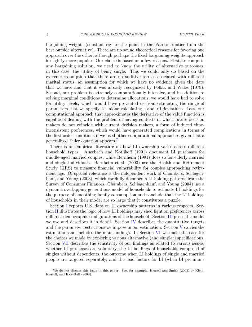
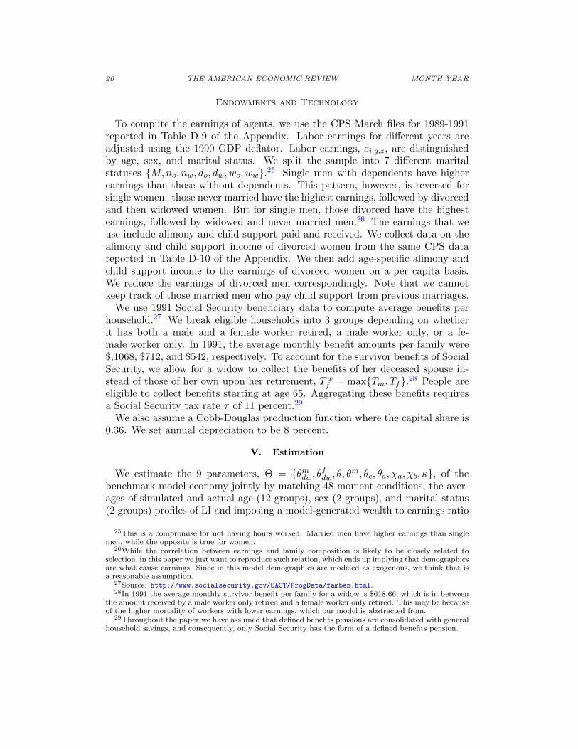
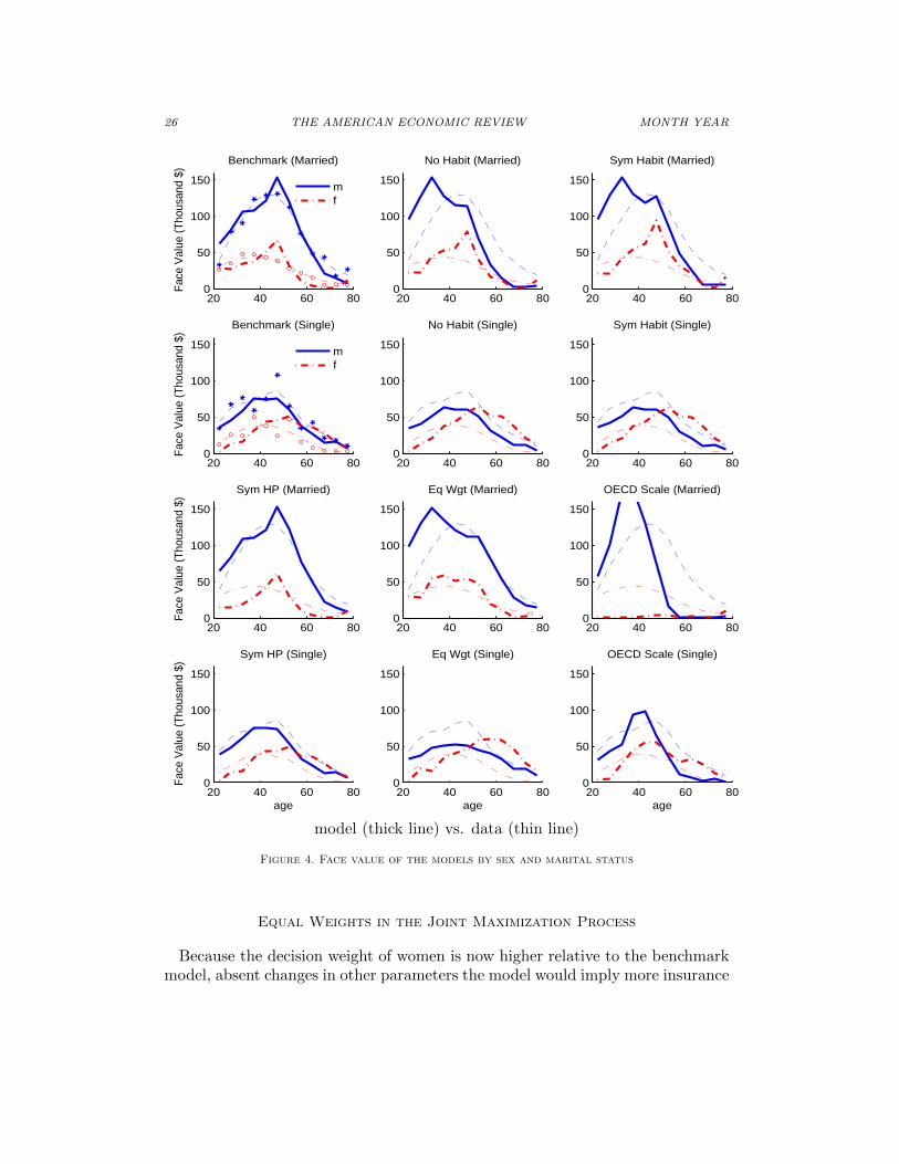
We explore the validity of our specification by abstracting sequentially the var-ious features included in the benchmark model. See Table 3 and Figure 4.
Marriage Does Not Generate Habits
In the benchmark model, the women’s habit parameter is significantly differentfrom zero, and we say that marriage generates strong habits for females. To
see the extent of this feature, we reestimate the model setting θmdw = θfdw =0, which implies that those who are divorced/widowed are not different fromthose who never married. All singles enjoy the same utility for a dollar spent.Compared with the benchmark model where women acquire strong habits whilein a marriage, this no-habit model generates too little LI holdings in the case ofa male’s death, especially later in his life relative to the data. In the absence ofhabits from marriage for women, married men do not need to hold much insurance.To account for the fact that married men hold 2.7 times more insurance thanmarried women, the newly estimated model attempts to tilt consumption towardmarried females by choosing a much lower decision weight for the male than inthe benchmark. To deal with the lower regard for consumption of older womenwithout habits, this version of the model attempts to lowers the bequest motiveintensity (χa). Overall, though, the quality of the estimates as measured by theSSE is notoriously worse than the benchmark’s, and we can reject the hypothesisof no habits at the 0.1 percent level based on the Wald test. This shows thathabits for women are needed to account for the large purchases of LI that occurlate in the husband’s life after most earnings have been made.
Marital Habits Are Symmetric between Men and Women
We also impose a symmetric structure in the habits created by marriage, θmdw =
θfdw. This is an intermediate case between the benchmark model and the restrictedmodel without habit. The restricted model predicts LI holdings for older malesthat are still too low, and we can reject the hypothesis of symmetric habits atthe 0.1 percent level. We conclude that it is hard to avoid the use of some formof habits to account for the LI purchases of older married men.
35All things equal, bequests are typically increasing in survival probability, and women’s survivaldifferential with men is increasing with age, which makes single women hold relatively more LI as theyget older.
VOL. VOL NO. ISSUE LIFE INSURANCE AND HOUSEHOLD CONSUMPTION 25
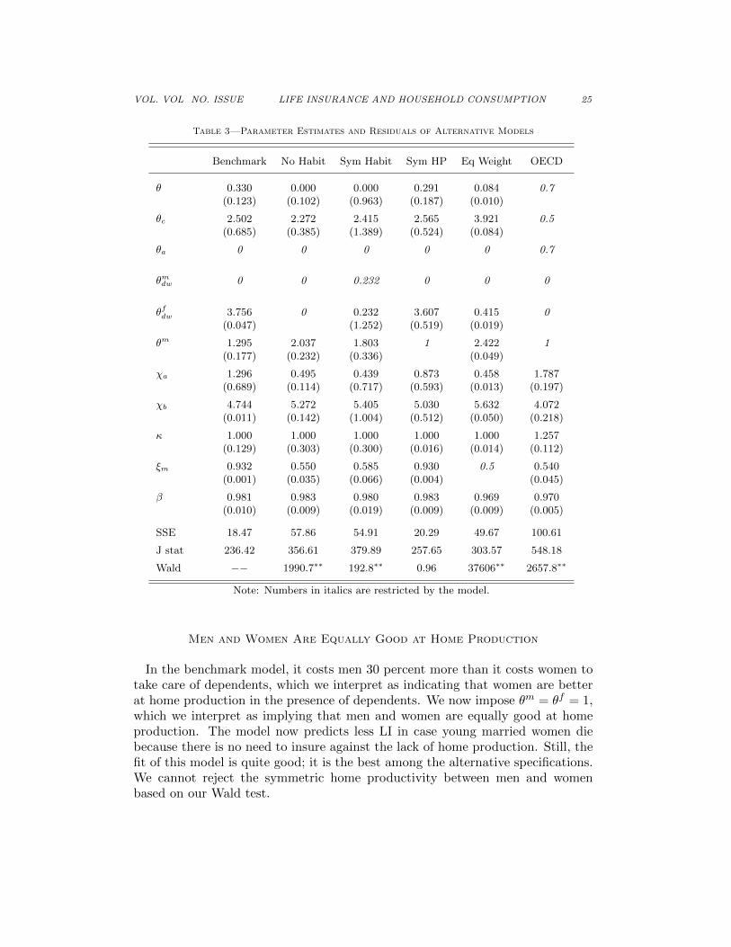
Table 3—Parameter Estimates and Residuals of Alternative Models
Benchmark No Habit Sym Habit Sym HP Eq Weight OECD
θ 0.330 0.000 0.000 0.291 0.084 0.7(0.123) (0.102) (0.963) (0.187) (0.010)
θc 2.502 2.272 2.415 2.565 3.921 0.5(0.685) (0.385) (1.389) (0.524) (0.084)
θa 0 0 0 0 0 0.7
θmdw 0 0 0.232 0 0 0
θfdw 3.756 0 0.232 3.607 0.415 0(0.047) (1.252) (0.519) (0.019)
θm 1.295 2.037 1.803 1 2.422 1(0.177) (0.232) (0.336) (0.049)
χa 1.296 0.495 0.439 0.873 0.458 1.787(0.689) (0.114) (0.717) (0.593) (0.013) (0.197)
χb 4.744 5.272 5.405 5.030 5.632 4.072(0.011) (0.142) (1.004) (0.512) (0.050) (0.218)
κ 1.000 1.000 1.000 1.000 1.000 1.257(0.129) (0.303) (0.300) (0.016) (0.014) (0.112)
ξm 0.932 0.550 0.585 0.930 0.5 0.540(0.001) (0.035) (0.066) (0.004) (0.045)
β 0.981 0.983 0.980 0.983 0.969 0.970(0.010) (0.009) (0.019) (0.009) (0.009) (0.005)
SSE 18.47 57.86 54.91 20.29 49.67 100.61
J stat 236.42 356.61 379.89 257.65 303.57 548.18
Wald −− 1990.7∗∗ 192.8∗∗ 0.96 37606∗∗ 2657.8∗∗
Note: Numbers in italics are restricted by the model.
Men and Women Are Equally Good at Home Production
In the benchmark model, it costs men 30 percent more than it costs women totake care of dependents, which we interpret as indicating that women are betterat home production in the presence of dependents. We now impose θm = θf = 1,which we interpret as implying that men and women are equally good at homeproduction. The model now predicts less LI in case young married women diebecause there is no need to insure against the lack of home production. Still, thefit of this model is quite good; it is the best among the alternative specifications.We cannot reject the symmetric home productivity between men and womenbased on our Wald test.
26 THE AMERICAN ECONOMIC REVIEW MONTH YEAR
20 40 60 800
50
100
150Fa
ce V
alue
(Tho
usan
d $)
Benchmark (Married)
mf
20 40 60 800
50
100
150
Face
Val
ue (T
hous
and
$)
Benchmark (Single)
mf
20 40 60 800
50
100
150
No Habit (Married)
20 40 60 800
50
100
150
No Habit (Single)
20 40 60 800
50
100
150
Sym Habit (Married)
20 40 60 800
50
100
150
Sym Habit (Single)
20 40 60 800
50
100
150
Sym HP (Married)
Face
Val
ue (T
hous
and
$)
20 40 60 800
50
100
150
Sym HP (Single)
Face
Val
ue (T
hous
and
$)
age
20 40 60 800
50
100
150
Eq Wgt (Married)
20 40 60 800
50
100
150
Eq Wgt (Single)
age
20 40 60 800
50
100
150
OECD Scale (Married)
20 40 60 800
50
100
150
OECD Scale (Single)
age
model (thick line) vs. data (thin line)
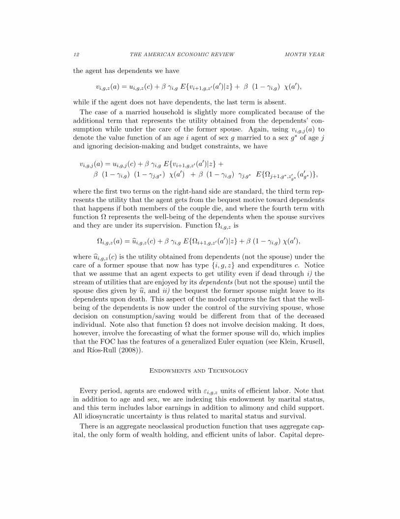
Figure 4. Face value of the models by sex and marital status
Equal Weights in the Joint Maximization Process
Because the decision weight of women is now higher relative to the benchmarkmodel, absent changes in other parameters the model would imply more insurance
VOL. VOL NO. ISSUE LIFE INSURANCE AND HOUSEHOLD CONSUMPTION 27
in case of a husband’s death and less in case of the wife’s death. The adjustmentis made by dramatically bumping up the men’s disadvantage at home production(142 percent versus 30 percent) and decreasing the marital habits for women(3.756 to 0.415). Even with these adjustments, the model predicts too much LIfor young husbands. The hypothesis of equal decision weights is rejected at the0.1 percent level.
The OECD Equivalence Scales
For the sake of comparison with a very standard measure of what a household is,we pose a version of the model that incorporates the OECD equivalence scales.36
To implement these ideas, we reestimate the patience and bequest parameters aswell as the weights in the joint maximization problem. The fit is worst amongvarious alternative specifications. The model predicts that insurance is held un-der circumstances that are different from those in which people in the UnitedStates hold insurance: the model underpredicts the holdings of married couples,especially late in life and conditional on the death of females. Notice that amongthe estimates, the curvature of the bequest function is much lower and the scaleparameter for the bequest function is much higher, which is the way in which thismodel increases insurance holdings.
The assessment of alternative models shows that abstracting from any of thefeatures of the benchmark model yields a much worse fit of the model (exceptperhaps for symmetric home production). We have explored many other versionsthat do not match the data well, but to avoid boring the reader, we do not reportthem. We have also shown that the OECD equivalence scales do a very bad jobin accounting for the patterns of holdings of LI.
VII. Other Modeling and Data Issues
We now turn to the sensitivity of our findings to various issues. All estimatesare shown in Table 4.
Voluntary Insurance
We also estimate the model to match the conservative measure of voluntaryinsurance introduced in Section I.A. In this case the model adapts to the slightlylower amounts of LI holdings by posing a lower value for the bequest intensityparameter χa (0.7 vs. 1.3) and a slightly higher weight for the husband in thehousehold’s decision problem ξ (0.95 vs 0.93). Even when we use this extremelyconservative measure of voluntary insurance, we still confirm our main findings:i) individuals are very caring for their dependents; ii) there are large economies of
36Under the OECD view (OECD (1982)), each additional adult in a household requires an expenditureof 70 cents in order to enjoy one dollar of consumption, while each child requires 50 cents. The OECDalso assumes that there are no habits or differences between males and females.
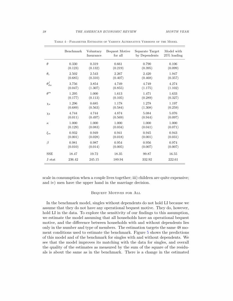
28 THE AMERICAN ECONOMIC REVIEW MONTH YEAR
Table 4—Parameter Estimates of Various Alternative Versions of the Model
Benchmark Voluntary Bequest Motive Separate Target Model withInsurance for all by Dependents 25% loading
θ 0.330 0.319 0.661 0.790 0.106(0.123) (0.132) (0.219) (0.395) (0.099)
θc 2.502 2.543 2.267 2.420 1.947(0.685) (0.310) (0.407) (0.468) (0.357)
θfdw 3.756 3.854 4.749 4.749 4.274(0.047) (1.307) (0.855) (1.175) (1.102)
θm 1.295 1.000 1.613 1.471 1.633(0.177) (0.113) (0.105) (0.289) (0.327)
χa 1.296 0.685 1.178 1.278 1.197(0.689) (0.563) (0.584) (1.308) (0.259)
χb 4.744 4.744 4.874 5.084 5.076(0.011) (0.497) (0.569) (0.944) (0.097)
κ 1.000 1.000 1.000 1.000 1.000(0.129) (0.083) (0.034) (0.041) (0.071)
ξm 0.932 0.949 0.941 0.945 0.943(0.001) (0.028) (0.018) (0.001) (0.031)
β 0.981 0.987 0.954 0.956 0.974(0.010) (0.014) (0.005) (0.007) (0.007)
SSE 18.47 19.72 18.35 99.87 16.55
J stat 236.42 245.15 189.94 332.92 222.61
scale in consumption when a couple lives together; iii) children are quite expensive;and iv) men have the upper hand in the marriage decision.
Bequest Motives for All
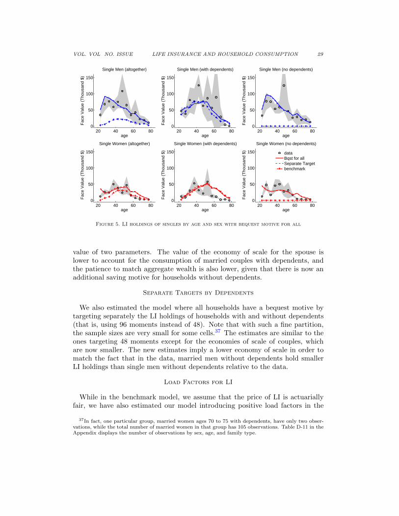
In the benchmark model, singles without dependents do not hold LI because weassume that they do not have any operational bequest motive. They do, however,hold LI in the data. To explore the sensitivity of our findings to this assumption,we estimate the model assuming that all households have an operational bequestmotive, and the difference between households with and without dependents liesonly in the number and type of members. The estimation targets the same 48 mo-ment conditions used to estimate the benchmark. Figure 5 shows the predictionsof this model and of the benchmark for singles with and without dependents. Wesee that the model improves its matching with the data for singles, and overallthe quality of the estimates as measured by the sum of the square of the residu-als is about the same as in the benchmark. There is a change in the estimated
VOL. VOL NO. ISSUE LIFE INSURANCE AND HOUSEHOLD CONSUMPTION 29
age
Fac
e V
alue
(T
hous
and
$)
Single Men (altogether)
20 40 60 800
50
100
150
age
Fac
e V
alue
(T
hous
and
$)
Single Men (with dependents)
20 40 60 800
50
100
150
age
Fac
e V
alue
(T
hous
and
$)
Single Men (no dependents)
20 40 60 800
50
100
150
age
Fac
e V
alue
(T
hous
and
$)
Single Women (altogether)
20 40 60 800
50
100
150
age
Fac
e V
alue
(T
hous
and
$)
Single Women (with dependents)
20 40 60 800
50
100
150
age
Fac
e V
alue
(T
hous
and
$)
Single Women (no dependents)
20 40 60 800
50
100
150 dataBqst for allSeparate Targetbenchmark
Figure 5. LI holdings of singles by age and sex with bequest motive for all
value of two parameters. The value of the economy of scale for the spouse islower to account for the consumption of married couples with dependents, andthe patience to match aggregate wealth is also lower, given that there is now anadditional saving motive for households without dependents.
Separate Targets by Dependents
We also estimated the model where all households have a bequest motive bytargeting separately the LI holdings of households with and without dependents(that is, using 96 moments instead of 48). Note that with such a fine partition,the sample sizes are very small for some cells.37 The estimates are similar to theones targeting 48 moments except for the economies of scale of couples, whichare now smaller. The new estimates imply a lower economy of scale in order tomatch the fact that in the data, married men without dependents hold smallerLI holdings than single men without dependents relative to the data.
Load Factors for LI
While in the benchmark model, we assume that the price of LI is actuariallyfair, we have also estimated our model introducing positive load factors in the
37In fact, one particular group, married women ages 70 to 75 with dependents, have only two obser-vations, while the total number of married women in that group has 105 observations. Table D-11 in theAppendix displays the number of observations by sex, age, and family type.
30 THE AMERICAN ECONOMIC REVIEW MONTH YEAR
insurance premium such that the premium is qi,g = (1+x)(1−γi,g), where x is theload factor set to 0.25.38 Again, the estimates are reported in Table 4. To accountfor the fact that married couples hold more life insurance than singles despite theunfair premium, the model predicts stronger economies of scale, θ = 0.106 relativeto 0.330 in the benchmark. The model also predicts a stronger marital habit for
women, θfdw = 4.274 (3.756 in the benchmark), to match the insurance holdingsof married men, and the estimate for the relative disadvantage of single men withdependents becomes larger, θm = 1.63 (1.30 in the benchmark), to match the factthat young married women hold significant amounts of life insurance.
VIII. Policy Experiment
We now proceed to look at a policy change that directly affects the nature ofincome streams depending on agents’ demographic circumstances. We abolishsurvivor’s benefits, which typically pay widows when their own Social Securityentitlement is lower than that of their deceased spouse.
In the benchmark model, a widow, once she reaches retirement age, collects thesame Social Security benefits of a male worker. This is our way of implementingthe current system of survivor’s benefits in the United States. We implement theabolition of survivor’s benefits as giving widows the same Social Security Benefitsthat never-married women receive (Twf = Tf ), which amounts to a 24 percentreduction in their benefits.
In the benchmark model, widows consume almost the same amount as marriedcouples due to the importance of the habits acquired by women in marriage, andthe death of an elderly husband acts as a drawback, since it implies lower incomebut not lower consumption. Eliminating survivor’s benefits is dealt with by anincrease in the amount of LI (payable when the male dies) purchased by thehousehold and not by a reduction of consumption by widows. Figure 6 displaysthe insurance face values in the benchmark model under the current policy andwithout survivor’s benefits. There is a noticeable increase in the holdings ofmarried men over age 50. Aggregate LI face value rises from 138 percent to 150percent of GDP. In addition to this effect on LI holdings, there is a 0.24 percentincrease in total assets.39
We also compute a compensated variation measure of welfare.40 Specifically, wecompute the ex ante discounted lifetime utility of newborns and calculate whatpercentage change in consumption makes agents indifferent between living in thebenchmark economy and living in an economy without survivor’s benefits.41 Note
38Mulligan and Philipson (2004) document the operating expense-premium ratios of five insurancecompanies, which range from 9 percent to 38 percent.
39This is under the small open economy assumption with constant interest rates.40This is not, strictly speaking, a welfare measure because it ignores the transition, except (almost)
for a cohort that is of age 20 at the time of the policy implementation.41The caveat made above about using estimates based on marginal conditions also applies here. How-
ever, given that the changes that we study are small, we think that the local information obtained issufficient to get a good idea of how the changes affect people.
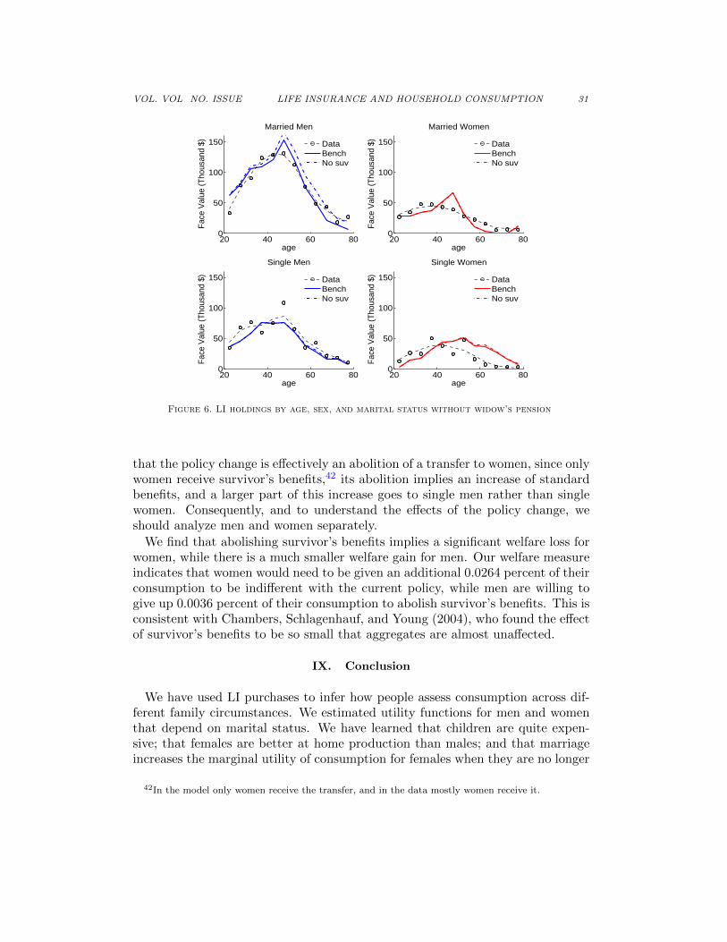
VOL. VOL NO. ISSUE LIFE INSURANCE AND HOUSEHOLD CONSUMPTION 31
20 40 60 800
50
100
150
age
Face
Val
ue (T
hous
and
$)
Married Men
DataBenchNo suv
20 40 60 800
50
100
150
age
Face
Val
ue (T
hous
and
$)
Married Women
DataBenchNo suv
20 40 60 800
50
100
150
age
Face
Val
ue (T
hous
and
$)
Single Men
DataBenchNo suv
20 40 60 800
50
100
150
age
Face
Val
ue (T
hous
and
$)
Single Women
DataBenchNo suv
Figure 6. LI holdings by age, sex, and marital status without widow’s pension
that the policy change is effectively an abolition of a transfer to women, since onlywomen receive survivor’s benefits,42 its abolition implies an increase of standardbenefits, and a larger part of this increase goes to single men rather than singlewomen. Consequently, and to understand the effects of the policy change, weshould analyze men and women separately.
We find that abolishing survivor’s benefits implies a significant welfare loss forwomen, while there is a much smaller welfare gain for men. Our welfare measureindicates that women would need to be given an additional 0.0264 percent of theirconsumption to be indifferent with the current policy, while men are willing togive up 0.0036 percent of their consumption to abolish survivor’s benefits. This isconsistent with Chambers, Schlagenhauf, and Young (2004), who found the effectof survivor’s benefits to be so small that aggregates are almost unaffected.
IX. Conclusion
We have used LI purchases to infer how people assess consumption across dif-ferent family circumstances. We estimated utility functions for men and womenthat depend on marital status. We have learned that children are quite expen-sive; that females are better at home production than males; and that marriageincreases the marginal utility of consumption for females when they are no longer
42In the model only women receive the transfer, and in the data mostly women receive it.
32 THE AMERICAN ECONOMIC REVIEW MONTH YEAR
married. With our estimates, we assessed the effects of some Social Security poli-cies, and we found that eliminating survivor’s benefits can be accommodated vialarger LI purchases in the case of the death of the male, but that it also impliesa small reduction in female well-being and a much smaller improvement in malewell-being.
Needless to say, this type of research has three immediate directions that callfor more work: i) the explicit modeling of time use, allowing for the possibility,not always exercised, of specialization in either market or home production activ-ities; ii) the consideration of more interesting decision-making processes withinthe household that essentially will imply that the weights depend on outside op-portunities that are time varying; and finally iii) the explicit consideration of theproblem of agents that differ in types (which may shed light on what is behindthe vast differences in the performance of single and married men, and that allowfor the consideration of education groups and of assortative matching). We arelooking forward to seeing more work in these directions.
REFERENCES
Aiyagari, S. Rao. 1994. “Uninsured Idiosyncratic Risk and Aggregate Saving.”Quarterly Journal of Economics, 109(3): 659–84.
Attanasio, Orazio P., and Martin Browning. 1995. “Consumption overthe Life Cycle and over the Business Cycle.” American Economic Review,85(5): 1118–37.
Attanasio, Orazio P., Hamish Low, and Virginia Sanchez-Marcos. 2008.“Explaining Changes in Female Labor Supply in a Life-cycle Model.” AmericanEconomic Review, 98(4): 1517–42.
Auerbach, Alan J., and Laurence J. Kotlikoff. 1991. “The Adequacy ofLife Insurance Purchases.” Journal of Financial Intermediation, 1(3): 215–41.
Bernheim, B. Douglas. 1991. “How Strong are Bequest Motives? EvidenceBased on Estimates of the Demand for Life Insurance and Annuities.” Journalof Political Economy, 99(5): 899–927.
Bernheim, B. Douglas, Lorenzo Forni, Jagadeesh Gokhale, and Lau-rence J. Kotlikoff. 2003. “The Mismatch between Life Insurance Holdingsand Financial Vulnerabilities: Evidence from the Health and Retirement Sur-vey.” American Economic Review, 93(1): 354–65.
Bewley, Truman. 1986. “Stationary Monetary Equilibrium with a Continuumof Independently Fluctuating Consumers.” In Contributions to MathematicalEconomics in Honor of Gerard Debreu, ed. Werner Hildenbrand and AndreuMas-Colell. Amsterdam: North Holland.
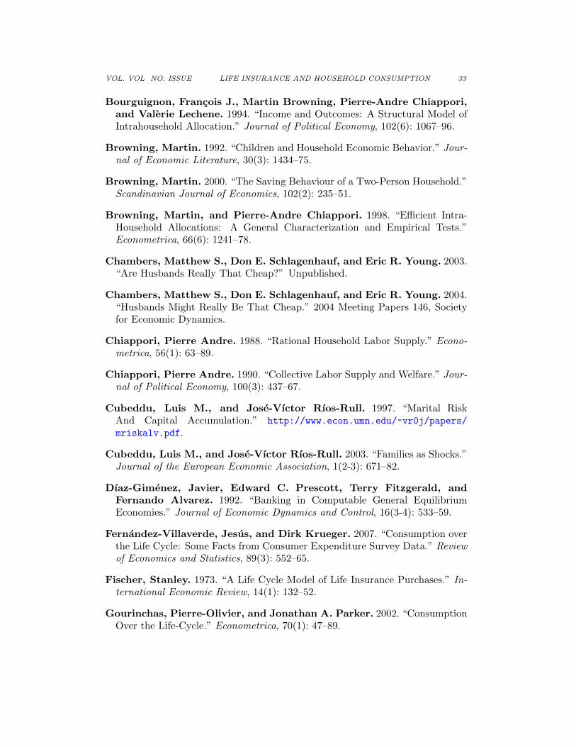
VOL. VOL NO. ISSUE LIFE INSURANCE AND HOUSEHOLD CONSUMPTION 33
Bourguignon, Francois J., Martin Browning, Pierre-Andre Chiappori,and Valerie Lechene. 1994. “Income and Outcomes: A Structural Model ofIntrahousehold Allocation.” Journal of Political Economy, 102(6): 1067–96.
Browning, Martin. 1992. “Children and Household Economic Behavior.” Jour-nal of Economic Literature, 30(3): 1434–75.
Browning, Martin. 2000. “The Saving Behaviour of a Two-Person Household.”Scandinavian Journal of Economics, 102(2): 235–51.
Browning, Martin, and Pierre-Andre Chiappori. 1998. “Efficient Intra-Household Allocations: A General Characterization and Empirical Tests.”Econometrica, 66(6): 1241–78.
Chambers, Matthew S., Don E. Schlagenhauf, and Eric R. Young. 2003.“Are Husbands Really That Cheap?” Unpublished.
Chambers, Matthew S., Don E. Schlagenhauf, and Eric R. Young. 2004.“Husbands Might Really Be That Cheap.” 2004 Meeting Papers 146, Societyfor Economic Dynamics.
Chiappori, Pierre Andre. 1988. “Rational Household Labor Supply.” Econo-metrica, 56(1): 63–89.
Chiappori, Pierre Andre. 1990. “Collective Labor Supply and Welfare.” Jour-nal of Political Economy, 100(3): 437–67.
Cubeddu, Luis M., and Jose-Vıctor Rıos-Rull. 1997. “Marital RiskAnd Capital Accumulation.” http://www.econ.umn.edu/~vr0j/papers/
mriskalv.pdf.
Cubeddu, Luis M., and Jose-Vıctor Rıos-Rull. 2003. “Families as Shocks.”Journal of the European Economic Association, 1(2-3): 671–82.
Dıaz-Gimenez, Javier, Edward C. Prescott, Terry Fitzgerald, andFernando Alvarez. 1992. “Banking in Computable General EquilibriumEconomies.” Journal of Economic Dynamics and Control, 16(3-4): 533–59.
Fernandez-Villaverde, Jesus, and Dirk Krueger. 2007. “Consumption overthe Life Cycle: Some Facts from Consumer Expenditure Survey Data.” Reviewof Economics and Statistics, 89(3): 552–65.
Fischer, Stanley. 1973. “A Life Cycle Model of Life Insurance Purchases.” In-ternational Economic Review, 14(1): 132–52.
Gourinchas, Pierre-Olivier, and Jonathan A. Parker. 2002. “ConsumptionOver the Life-Cycle.” Econometrica, 70(1): 47–89.
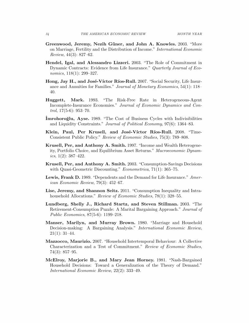
34 THE AMERICAN ECONOMIC REVIEW MONTH YEAR
Greenwood, Jeremy, Nezih Guner, and John A. Knowles. 2003. “Moreon Marriage, Fertility and the Distribution of Income.” International EconomicReview, 44(3): 827–62.
Hendel, Igal, and Alessandro Lizzeri. 2003. “The Role of Commitment inDynamic Contracts: Evidence from Life Insurance.” Quarterly Journal of Eco-nomics, 118(1): 299–327.
Hong, Jay H., and Jose-Vıctor Rıos-Rull. 2007. “Social Security, Life Insur-ance and Annuities for Families.” Journal of Monetary Economics, 54(1): 118–40.
Huggett, Mark. 1993. “The Risk-Free Rate in Heterogeneous-AgentIncomplete-Insurance Economies.” Journal of Economic Dynamics and Con-trol, 17(5-6): 953–70.
Imrohoroglu, Ayse. 1989. “The Cost of Business Cycles with Indivisibilitiesand Liquidity Constraints.” Journal of Political Economy, 97(6): 1364–83.
Klein, Paul, Per Krusell, and Jose-Vıctor Rıos-Rull. 2008. “Time-Consistent Public Policy.” Review of Economic Studies, 75(3): 789–808.
Krusell, Per, and Anthony A. Smith. 1997. “Income and Wealth Heterogene-ity, Portfolio Choice, and Equilibrium Asset Returns.” Macroeconomic Dynam-ics, 1(2): 387–422.
Krusell, Per, and Anthony A. Smith. 2003. “Consumption-Savings Decisionswith Quasi-Geometric Discounting.” Econometrica, 71(1): 365–75.
Lewis, Frank D. 1989. “Dependents and the Demand for Life Insurance.” Amer-ican Economic Review, 79(3): 452–67.
Lise, Jeremy, and Shannon Seitz. 2011. “Consumption Inequality and Intra-household Allocations.” Review of Economic Studies, 78(1): 328–55.
Lundberg, Shelly J., Richard Startz, and Steven Stillman. 2003. “TheRetirement-Consumption Puzzle: A Marital Bargaining Approach.” Journal ofPublic Economics, 87(5-6): 1199–218.
Manser, Marilyn, and Murray Brown. 1980. “Marriage and HouseholdDecision-making: A Bargaining Analysis.” International Economic Review,21(1): 31–44.
Mazzocco, Maurizio. 2007. “Household Intertemporal Behaviour: A CollectiveCharacterization and a Test of Commitment.” Review of Economic Studies,74(3): 857–95.
McElroy, Marjorie B., and Mary Jean Horney. 1981. “Nash-BargainedHousehold Decisions: Toward a Generalization of the Theory of Demand.”International Economic Review, 22(2): 333–49.
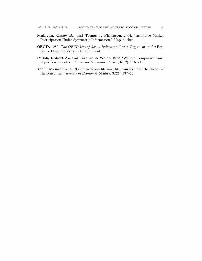
VOL. VOL NO. ISSUE LIFE INSURANCE AND HOUSEHOLD CONSUMPTION 35
Mulligan, Casey B., and Tomas J. Philipson. 2004. “Insurance MarketParticipation Under Symmetric Information.” Unpublished.
OECD. 1982. The OECD List of Social Indicators. Paris: Organization for Eco-nomic Co-operation and Development.
Pollak, Robert A., and Terence J. Wales. 1979. “Welfare Comparisons andEquivalence Scales.” American Economic Review, 69(2): 216–21.
Yaari, Menahem E. 1965. “Uncertain lifetime, life insurance and the theory ofthe consumer.” Review of Economic Studies, 32(2): 137–50.