lie groups, condensed - perimeter institute · theorem 2.14 inverse mapping theorem ... with the...
TRANSCRIPT

Lie Groups and Lie Algebras
this document by Theo Johnson-Freydbased on: Mark Haiman, Math 261A: Lie Groups
Fall 2008, UC-Berkeley
Last updated December 23, 2009

ii

Contents
Contents vList of Theorems . . . . . . . . . . . . . . . . . . . . . . . . . . . . . . . . . . . . . . . . . v
Introduction vii0.1 Notation . . . . . . . . . . . . . . . . . . . . . . . . . . . . . . . . . . . . . . . . . . . vii
1 Motivation: Closed Linear Groups 11.1 Definition of a Lie Group . . . . . . . . . . . . . . . . . . . . . . . . . . . . . . . . . 1
1.1.1 Group objects . . . . . . . . . . . . . . . . . . . . . . . . . . . . . . . . . . . . 11.1.2 Analytic and Algebraic Groups . . . . . . . . . . . . . . . . . . . . . . . . . . 2
1.2 Definition of a Closed Linear Group . . . . . . . . . . . . . . . . . . . . . . . . . . . 31.2.1 Lie algebra of a closed linear group . . . . . . . . . . . . . . . . . . . . . . . . 31.2.2 Some analysis . . . . . . . . . . . . . . . . . . . . . . . . . . . . . . . . . . . . 4
1.3 Classical Lie groups . . . . . . . . . . . . . . . . . . . . . . . . . . . . . . . . . . . . 51.3.1 Classical Compact Lie groups . . . . . . . . . . . . . . . . . . . . . . . . . . . 51.3.2 Classical Complex Lie groups . . . . . . . . . . . . . . . . . . . . . . . . . . . 51.3.3 The Classical groups . . . . . . . . . . . . . . . . . . . . . . . . . . . . . . . . 6
1.4 Homomorphisms of closed linear groups . . . . . . . . . . . . . . . . . . . . . . . . . 6Exercises . . . . . . . . . . . . . . . . . . . . . . . . . . . . . . . . . . . . . . . . . . . . . 7
2 Mini-course in Differential Geometry 92.1 Manifolds . . . . . . . . . . . . . . . . . . . . . . . . . . . . . . . . . . . . . . . . . . 9
2.1.1 Classical definition . . . . . . . . . . . . . . . . . . . . . . . . . . . . . . . . . 92.1.2 Sheafs . . . . . . . . . . . . . . . . . . . . . . . . . . . . . . . . . . . . . . . . 102.1.3 Manifold constructions . . . . . . . . . . . . . . . . . . . . . . . . . . . . . . . 102.1.4 Submanifolds . . . . . . . . . . . . . . . . . . . . . . . . . . . . . . . . . . . . 11
2.2 Vector Fields . . . . . . . . . . . . . . . . . . . . . . . . . . . . . . . . . . . . . . . . 122.2.1 Definition . . . . . . . . . . . . . . . . . . . . . . . . . . . . . . . . . . . . . . 122.2.2 Integral Curves . . . . . . . . . . . . . . . . . . . . . . . . . . . . . . . . . . . 132.2.3 Group Actions . . . . . . . . . . . . . . . . . . . . . . . . . . . . . . . . . . . 142.2.4 Lie algebra of a Lie group . . . . . . . . . . . . . . . . . . . . . . . . . . . . . 15
Exercises . . . . . . . . . . . . . . . . . . . . . . . . . . . . . . . . . . . . . . . . . . . . . 16
iii

iv CONTENTS
3 General theory of Lie groups 193.1 From Lie algebra to Lie group . . . . . . . . . . . . . . . . . . . . . . . . . . . . . . . 19
3.1.1 The exponential map . . . . . . . . . . . . . . . . . . . . . . . . . . . . . . . . 193.1.2 The Fundamental Theorem . . . . . . . . . . . . . . . . . . . . . . . . . . . . 20
3.2 Universal Enveloping Algebras . . . . . . . . . . . . . . . . . . . . . . . . . . . . . . 223.2.1 The Definition . . . . . . . . . . . . . . . . . . . . . . . . . . . . . . . . . . . 223.2.2 Poincare-Birkhoff-Witt Theorem . . . . . . . . . . . . . . . . . . . . . . . . . 243.2.3 Ug is a bialgebra . . . . . . . . . . . . . . . . . . . . . . . . . . . . . . . . . . 253.2.4 Geometry of the Universal Enveloping Algebra . . . . . . . . . . . . . . . . . 26
3.3 The Baker-Campbell-Hausdorff Formula . . . . . . . . . . . . . . . . . . . . . . . . . 263.4 Lie Subgroups . . . . . . . . . . . . . . . . . . . . . . . . . . . . . . . . . . . . . . . . 28
3.4.1 Relationship between Lie subgroups and Lie subalgebras . . . . . . . . . . . . 283.4.2 Review of Algebraic Topology . . . . . . . . . . . . . . . . . . . . . . . . . . . 30
3.5 A dictionary between algebras and groups . . . . . . . . . . . . . . . . . . . . . . . . 323.5.1 Basic Examples: one- and two-dimensional Lie algebras . . . . . . . . . . . . 33
Exercises . . . . . . . . . . . . . . . . . . . . . . . . . . . . . . . . . . . . . . . . . . . . . 34
4 General theory of Lie algebras 394.1 Ug is a Hopf algebra . . . . . . . . . . . . . . . . . . . . . . . . . . . . . . . . . . . . 394.2 Structure Theory of Lie Algebras . . . . . . . . . . . . . . . . . . . . . . . . . . . . . 41
4.2.1 Many Definitions . . . . . . . . . . . . . . . . . . . . . . . . . . . . . . . . . . 414.2.2 Nilpotency: Engel’s Theorem and Corollaries . . . . . . . . . . . . . . . . . . 424.2.3 Solvability: Lie’s Theorem and Corollaries . . . . . . . . . . . . . . . . . . . . 434.2.4 The Killing Form . . . . . . . . . . . . . . . . . . . . . . . . . . . . . . . . . . 444.2.5 Jordan Form . . . . . . . . . . . . . . . . . . . . . . . . . . . . . . . . . . . . 454.2.6 Cartan’s Criteria . . . . . . . . . . . . . . . . . . . . . . . . . . . . . . . . . . 47
4.3 Examples: three-dimensional Lie algebras . . . . . . . . . . . . . . . . . . . . . . . . 484.4 Some Homological Algebra . . . . . . . . . . . . . . . . . . . . . . . . . . . . . . . . 48
4.4.1 The Casimir . . . . . . . . . . . . . . . . . . . . . . . . . . . . . . . . . . . . 494.4.2 Review of Ext . . . . . . . . . . . . . . . . . . . . . . . . . . . . . . . . . . . 494.4.3 Complete Reducibility . . . . . . . . . . . . . . . . . . . . . . . . . . . . . . . 514.4.4 Computing Exti(K,M) . . . . . . . . . . . . . . . . . . . . . . . . . . . . . . 52
4.5 From Zassenhaus to Ado . . . . . . . . . . . . . . . . . . . . . . . . . . . . . . . . . . 55Exercises . . . . . . . . . . . . . . . . . . . . . . . . . . . . . . . . . . . . . . . . . . . . . 59
5 Classification of Semisimple Lie Algebras 635.1 Classical Lie algebras over C . . . . . . . . . . . . . . . . . . . . . . . . . . . . . . . 63
5.1.1 Reductive Lie algebras . . . . . . . . . . . . . . . . . . . . . . . . . . . . . . . 635.1.2 Guiding examples: sl(n) and sp(n) over C . . . . . . . . . . . . . . . . . . . . 64
5.2 Representation Theory of sl(2) . . . . . . . . . . . . . . . . . . . . . . . . . . . . . . 705.3 Cartan subalgebras . . . . . . . . . . . . . . . . . . . . . . . . . . . . . . . . . . . . . 72
5.3.1 Definition and Existence . . . . . . . . . . . . . . . . . . . . . . . . . . . . . . 725.3.2 More on the Jordan Decomposition and Schur’s Lemma . . . . . . . . . . . . 755.3.3 Precise description of Cartan subalgebras . . . . . . . . . . . . . . . . . . . . 77

CONTENTS v
5.4 Root systems . . . . . . . . . . . . . . . . . . . . . . . . . . . . . . . . . . . . . . . . 785.4.1 Motivation and a Quick Computation . . . . . . . . . . . . . . . . . . . . . . 785.4.2 The Definition . . . . . . . . . . . . . . . . . . . . . . . . . . . . . . . . . . . 795.4.3 Classification of rank-two root systems . . . . . . . . . . . . . . . . . . . . . . 805.4.4 Positive roots . . . . . . . . . . . . . . . . . . . . . . . . . . . . . . . . . . . . 83
5.5 Cartan Matrices and Dynkin Diagrams . . . . . . . . . . . . . . . . . . . . . . . . . . 845.5.1 Definitions . . . . . . . . . . . . . . . . . . . . . . . . . . . . . . . . . . . . . 845.5.2 Classification of finite-type Cartan matrices . . . . . . . . . . . . . . . . . . . 85
5.6 From Cartan Matrix to Lie Algebra . . . . . . . . . . . . . . . . . . . . . . . . . . . 90Exercises . . . . . . . . . . . . . . . . . . . . . . . . . . . . . . . . . . . . . . . . . . . . . 94
6 Representation Theory of Semisimple Lie Groups 996.1 Irreducible Lie-algebra representations . . . . . . . . . . . . . . . . . . . . . . . . . . 996.2 Algebraic Lie Groups . . . . . . . . . . . . . . . . . . . . . . . . . . . . . . . . . . . . 108
6.2.1 Guiding example: SL(n) and PSL(n) . . . . . . . . . . . . . . . . . . . . . . . 1086.2.2 Definition and General Properties of Algebraic Groups . . . . . . . . . . . . . 1106.2.3 Constructing G from g . . . . . . . . . . . . . . . . . . . . . . . . . . . . . . . 113
6.3 Conclusion . . . . . . . . . . . . . . . . . . . . . . . . . . . . . . . . . . . . . . . . . 117Exercises . . . . . . . . . . . . . . . . . . . . . . . . . . . . . . . . . . . . . . . . . . . . . 119
Index 121
Bibliography 125
List of Theorems
Theorem 2.14 Inverse Mapping Theorem . . . . . . . . . . . . . . . . . . . . . . . . . . . . . 11Theorem 3.5 Exponential Map . . . . . . . . . . . . . . . . . . . . . . . . . . . . . . . . . . 20Theorem 3.12 Fundamental Theorem of Lie Groups and Algebras . . . . . . . . . . . . . . . 20Theorem 3.14 Baker-Campbell-Hausdorff Formula (second part only) . . . . . . . . . . . . . 21Theorem 3.24 Poincare-Birkhoff-Witt . . . . . . . . . . . . . . . . . . . . . . . . . . . . . . . 24Theorem 3.31 Grothendieck Differential Operators . . . . . . . . . . . . . . . . . . . . . . . . 26Theorem 3.35 Baker-Campbell-Hausdorff Formula . . . . . . . . . . . . . . . . . . . . . . . . 27Theorem 3.37 Identification of Lie subalgebras and Lie subgroups . . . . . . . . . . . . . . . 28Theorem 4.25 Engel’s Theorem . . . . . . . . . . . . . . . . . . . . . . . . . . . . . . . . . . . 42Theorem 4.37 Lie’s Theorem . . . . . . . . . . . . . . . . . . . . . . . . . . . . . . . . . . . . 43Theorem 4.50 Jordan decomposition . . . . . . . . . . . . . . . . . . . . . . . . . . . . . . . . 45Theorem 4.53 Cartan’s First Criterion . . . . . . . . . . . . . . . . . . . . . . . . . . . . . . . 47Theorem 4.55 Cartan’s Second Criterian . . . . . . . . . . . . . . . . . . . . . . . . . . . . . 47Theorem 4.74 Schur’s Lemma . . . . . . . . . . . . . . . . . . . . . . . . . . . . . . . . . . . . 51Theorem 4.76 Ext1 vanishes over a semisimple Lie algebra . . . . . . . . . . . . . . . . . . . 52Theorem 4.78 Weyl’s Complete Reducibility Theorem . . . . . . . . . . . . . . . . . . . . . . 52Theorem 4.79 Whitehead’s Theorem . . . . . . . . . . . . . . . . . . . . . . . . . . . . . . . . 52

vi CONTENTS
Theorem 4.86 Levi’s Theorem . . . . . . . . . . . . . . . . . . . . . . . . . . . . . . . . . . . 54Theorem 4.88 Malcev-Harish-Chandra Theorem . . . . . . . . . . . . . . . . . . . . . . . . . 55Theorem 4.89 Lie’s Third Theorem . . . . . . . . . . . . . . . . . . . . . . . . . . . . . . . . 55Theorem 4.97 Zassenhaus’s Extension Lemma . . . . . . . . . . . . . . . . . . . . . . . . . . 57Theorem 4.99 Ado’s Theorem . . . . . . . . . . . . . . . . . . . . . . . . . . . . . . . . . . . 58Theorem 5.27 Existence of a Cartan Subalgebra . . . . . . . . . . . . . . . . . . . . . . . . . 74Theorem 5.35 Schur’s Lemma over an algebraically closed field . . . . . . . . . . . . . . . . . 76Theorem 5.79 Classification of indecomposable Dynkin diagrams . . . . . . . . . . . . . . . . 89Theorem 5.89 Serre Relations . . . . . . . . . . . . . . . . . . . . . . . . . . . . . . . . . . . . 92Theorem 5.94 Classification of finite-dimensional simple Lie algebras . . . . . . . . . . . . . . 93Theorem 6.15 Weyl Character Formula . . . . . . . . . . . . . . . . . . . . . . . . . . . . . . 103Theorem 6.24 Weyl Dimension Formula . . . . . . . . . . . . . . . . . . . . . . . . . . . . . . 106Theorem 6.69 Semisimple Lie algebras are algebraically integrable . . . . . . . . . . . . . . . 116Theorem 6.70 Classification of Semisimple Lie Groups over C . . . . . . . . . . . . . . . . . . 117

Introduction
In the Fall Semester, 2008, Prof. Mark Haiman taught Math 261A: Lie Groups, at the Universityof California Berkeley. The course covered the structure of Lie groups, Lie algebras, and their(complex) representations. The textbooks were [2] and [11]. I was one of many students in thatclass, and typed detailed notes [8], including all the motivation, discussion, questions, errors, andpersonal confusions and commentary. What you’re reading right now is a first attempt to makethose notes more presentable. It is also a study aid for my qualifying exam. As such, we present onlythe definitions, theorems, and proofs, with little motivation. I have made limited rearrangementsof the material. Each subsection corresponds to one or two one-hour lectures. Needless to say,the pedagogy (and, since I was taking dictation, many of the words), are due to M. Haiman. Inparticular, I have quoted almost verbatim the problem sets M. Haiman assigned in the class (thereader may find my answers to some of the exercises in the appendices of [8]). Of course, any andall errors are mine.
In addition to [2, 11], the reader might be interested in getting a sense of previous renditionsof UC Berkeley’s Math 261. In 2006 a three-professor tag-team taught a one-semester Lie Groupsand Lie Algebras course; detailed notes are available [18], and occasionally I have referenced thosenotes, especially when I was absent or lost, or when my notes are otherwise lacking. They goquickly through the material — about twice as fast as we did — eschewing most proofs. For a verydifferent version of the course, the reader may be interested in the year-long Lie Groups and LieAlgebras course taught in 2001 [12].
These notes are typeset using TEXShop Pro on a MacBook running OS 10.5; the backend ispdfLATEX. Pictures and diagrams are drawn using pgf/TikZ. For a full list of packages used, youmay peruse the LATEX source code for this document, available at http://math.berkeley.edu/
~theojf/LieGroupsBook.tex.In addition to Mark Haiman, the people without whom I would not have been able to put
together this text were Alex Fink, Dustin Cartwright, Manuel Reyes, and the other participants inthe class.
0.1 Notation
We will generally use A,B, C, . . . for categories; named categories are written in small-caps, so thatfor example A-mod is the category of (finite-dimensional) A-modules. Objects in a category aregenerally denoted A,B,C, . . . , with the exception that for Lie algebras we use fraktur letters a, b, c.The classical Lie groups we refer to with roman letters (GL(n,C), etc.), and we write M(n) for
vii

viii CONTENTS
the algebra of n× n matrices. Famous fields and rings are in black-board-bold: R,C,Q,Z, and weuse K rather than k for a generic field. The natural numbers N is always the set of non-negativeintegers, so that it is a rig, or “ring with identities but without negations”.
In a category with products, we use {pt} for the terminal object, and × for the monoidalstructure; a general monoidal category is written with ⊗ for the product. We do not includeassociators and other higher-categorical things.
For morphisms in a category we use lower-case Greek and Roman letters α, β, a, b, c, . . . . Anelement of an object A in monoidal category is a morphism a : {pt} → A, or with {pt} replacedby the monoidal unit; we will write this as “a ∈ A” following the usual convention. When thecategory is concrete with products, this agrees with the set-theoretic meaning. The identity mapon any object A ∈ A we write as 1A. We always write the identity matrix as 1, or 1n for the n× nidentity matrix when we need to specify its size. Similarly, 0 and 0n refer to the zero matrix.
If M is a manifold (we will never need more general geometric spaces), we will write C (M)for the continuous, smooth, analytic, or holomorphic functions on it, depending on what is naturalfor the given space. Thus if M is a real manifold, we will always use the symbol C for thesheaf of infinitely-differentiable or analytic functions on it, depending on whether the ambientcategory is that of infinitely-differentiable manifolds or analytic manifolds. When working overthe complex numbers, C may refer to the sheaf of complex analytic functions or of holomorphicfunctions. Moreover, the word “smooth” may mean any of “infinitely-differentiable”, “analytic”,or “holomorphic”, depending on the choice of ambient category. When a statement does not holdin this generality, we will specify. We write TM for the tangent bundle of M , and TpM for thefiber over the point p.

Chapter 1
Motivation: Closed Linear Groups
1.1 Definition of a Lie Group
[8, Lecture 1]
1.1.1 Group objects
1.1 Definition Let C be a category with finite products; denote the terminal object by {pt}. Agroup object in C is an object G along with maps µ : G × G → G, i : G → G, and e : {pt} → G,such that the following diagrams commute:
G×G×G G×G
G×G G
1G×µ
µ×1G µ
µ
(1.1.1)
G{pt} ×G
G×G
G× {pt}
e×1Gµ
∼
1G×e
∼
(1.1.2)
{pt}G
G×G G×G
G
G×G G×G
e
∆
∆
µ
µ
1G×i
i×1G
(1.1.3)
1

2 CHAPTER 1. MOTIVATION: CLOSED LINEAR GROUPS
In equation 1.1.2, the isomorphisms are the canonical ones. In equation 1.1.3, the map G→ {pt}is the unique map to the terminal object, and ∆ : G→ G×G is the canonical diagonal map.
If (G,µG, eG, iG) and (H,µH , eH , iH) are two group objects, a map f : G→ H is a group objecthomomorphism if the following commute:
G×G G
H ×H H
µG
µH
f×f f {pt}
G
H
eG
eH
f (1.1.4)
(That f intertwines iG with iH is then a corollary.)
1.2 Definition A (left) group action of a group object G in a category C with finite products is amap ρ : G×X → X such that the following diagrams commute:
G×G×X G×X
G×X X
1G×ρ
µ×1X ρ
ρ
(1.1.5)
X
G×X
{pt} ×X
ρe×1X
∼
(1.1.6)
(The diagram corresponding to equation 1.1.3 is then a corollary.) A right action is a map X×G→X with similar diagrams. We denote a left group action ρ : G×X → X by ρ : Gy X.
Let ρX : G × X → X and ρY : G × Y → Y be two group actions. A map f : X → Y isG-equivariant if the following square commutes:
G×X X
G× Y Y
ρX
1G×f f
ρY
(1.1.7)
1.1.2 Analytic and Algebraic Groups
1.3 Definition A Lie group is a group object in a category of manifolds. In particular, a Lie groupcan be infinitely differentiable (in the category C∞-Man) or analytic (in the category C ω-Man)

1.2. DEFINITION OF A CLOSED LINEAR GROUP 3
when over R, or complex analytic or almost complex when over C. We will take “Lie group” tomean analytic Lie group over either C or R. In fact, the different notions of real Lie group coincide,a fact that we will not directly prove, as do the different notions of complex Lie group. As always,we will use the word “smooth” for any of “infinitely differentiable”, “analytic”, or “holomorphic”.
A Lie action is a group action in the category of manifolds.A (linear) algebraic group over K (algebraically closed) is a group object in the category of
(affine) algebraic varieties over K.
1.4 Example The general linear group GL(n,K) of n×n invertible matrices is a Lie group over Kfor K = R or C. When K is algebraically closed, GL(n,K) is an algebraic group. It acts algebraicallyon Kn and on projective space P(Kn) = Pn−1(K).
1.2 Definition of a Closed Linear Group
[8, Lectures 2 and 3]We write GL(n,K) for the group of n×n invertible matrices over K, and M(n,K) for the algebra
of all n× n matrices. We regularly leave off the K.
1.5 Definition A closed linear group is a subgroup of GL(n) (over C or R) that is closed as atopological subspace.
1.2.1 Lie algebra of a closed linear group
1.6 Lemma / Definition The following describe the same function exp : M(n) → GL(n), calledthe matrix exponential.
1. exp(a) def=∑n≥0
an
n!.
2. exp(a) def= eta∣∣∣t=1
, where for fixed a ∈ M(n) we define eta as the solution to the initial value
problem e0a = 1, ddte
ta = aeta.
3. exp(a) def= limn→∞
Å1 +
a
n
ãn.
If ab− ba = 0, then exp(a+ b) = exp(a) + exp(b).The function exp : M(n)→ GL(n) is a local isomorphism of analytic manifolds. In a neighbor-
hood of 1 ∈ GL(n), the function log a def= −∑n>0
(1− a)n
nis an inverse to exp.
1.7 Lemma / Definition Let H be a closed linear group. The Lie algebra of H is the set
Lie(H) = {x ∈ M(n) : exp(Rx) ⊆ H} (1.2.1)
1. Lie(H) is a R-subspace of M(n).

4 CHAPTER 1. MOTIVATION: CLOSED LINEAR GROUPS
2. Lie(H) is closed under the bracket [, ] : (a, b) 7→ ab− ba.
1.8 Definition A Lie algebra over K is a vector space g along with an antisymmetric map [, ] :g⊗ g→ g satisfying the Jacobi identity:
[[a, b], c] + [[b, c], a] + [[c, a], b] = 0 (1.2.2)
A homomorphism of Lie algebras is a linear map preserving the bracket. A Lie subalgebra is avector subspace closed under the bracket.
1.9 Example The algebra gl(n) = M(n) of n × n matrices is a Lie algebra with [a, b] = ab − ba.It is Lie(GL(n)). Lemma/Definition 1.7 says that Lie(H) is a Lie subalgebra of M(n).
1.2.2 Some analysis
1.10 Lemma Let M(n) = V ⊕W as a real vector space. Then there exists an open neighborhoodU 3 0 in M(n) and an open neighborhood U ′ 3 1 in GL(n) such that (v, w) 7→ exp(v) exp(w) :V ⊕W → GL(n) is a homeomorphism U → U ′.
1.11 Lemma Let H be a closed subgroup of GL(n), and W ⊆ M(n) be a linear subspace such that0 is a limit point of the set {w ∈W s.t. exp(w) ∈ H}. Then W ∩ Lie(H) 6= 0.
Proof Fix a Euclidian norm on W . Let w1, w2, · · · → 0 be a sequence in {w ∈W s.t. exp(w) ∈ H},with wi 6= 0. Then wi/|wi| are on the unit sphere, which is compact, so passing to a subsequence,we can assume that wi/|wi| → x where x is a unit vector. The norms |wi| are tending to 0, sowi/|wi| is a large multiple of wi. We approximate this: let ni = d1/|wi|e, whence niwi ≈ wi/|wi|,and niwi → x. But expwi ∈ H, so exp(niwi) ∈ H, and H is a closed subgroup, so expx ∈ H.
Repeating the argument with a ball of radius r to conclude that exp(rx) is in H, we concludethat x ∈ Lie(H). �
1.12 Proposition Let H be a closed subgroup of GL(n). There exist neighborhoods 0 ∈ U ⊆ M(n)and 1 ∈ U ′ ⊆ GL(n) such that exp : U ∼→ U ′ takes Lie(H) ∩ U ∼→ H ∩ U ′.
Proof We fix a complement W ⊆ M(n) such that M(n) = Lie(H) ⊕W . By Lemma 1.11, we canfind a neighborhood V ⊆ W of 0 such that {v ∈ V s.t. exp(v) ∈ H} = {0}. Then on Lie(H)× V ,the map (x,w) 7→ exp(x) exp(w) lands in H if and only if w = 0. By restricting the first componentto lie in an open neighborhood, we can approximate exp(x+w) ≈ exp(x) exp(w) as well as we needto — there’s a change of coordinates that completes the proof. �
1.13 Corollary H is a submanifold of GL(n) of dimension equal to the dimension of Lie(H).
1.14 Corollary exp(Lie(H)) generates the identity component H0 of H.
1.15 Remark In any topological group, the connected component of the identity is normal.
1.16 Corollary Lie(H) is the tangent space T1Hdef= {γ′(0) s.t. γ : R→ H, γ(0) = 1} ⊆ M(n).

1.3. CLASSICAL LIE GROUPS 5
1.3 Classical Lie groups
[8, Lectures 4 and 5]We mention only the classical compact semisimple Lie groups and the classical complex semisim-
ple Lie groups. There are other very interesting classical Lie groups, c.f. [14].
1.3.1 Classical Compact Lie groups
1.17 Lemma / Definition The quaternians H is the unital R-algebra generated by i, j, k with themultiplication i2 = j2 = k2 = ijk = −1; it is a non-commutative division ring. Then R ↪→ C ↪→ H,and H is a subalgebra of M(4,R). We defined the complex conjugate linearly by i = −i, j = −j, andk = −k; complex conjugation is an anti-automorphism, and the fixed-point set is R. The Euclideannorm of ζ ∈ H is given by ‖ζ‖ = ζζ.
The Euclidean norm of a column vector x ∈ Rn,Cn,Hn is given by ‖x‖2 = xTx, where x is thecomponent-wise complex conjugation of x.
If x ∈ M(n,R),M(n,C),M(n,H) is a matrix, we define its Hermetian conjugate to be the matrixx∗ = xT ; Hermetian conjugation is an antiautomorphism of algebras M(n) → M(n). M(n,H) ↪→M(2n,C) is a ∗-embedding.
Let j =Ç
0 −11 0
å∈ M(2,M(n,C)) = M(2n,C) be a block matrix. We define GL(n,H) def=
{x ∈ GL(2n,C) s.t. jx = xj}. It is a closed linear group.
1.18 Lemma / Definition The following are closed linear groups, and are compact:
• The (real) special orthogonal group SO(n,R) def= {x ∈ M(n,R) s.t. x∗x = 1 and detx = 1}.
• The (real) orthogonal group O(n,R) def= {x ∈ M(n,R) s.t. x∗x = 1}.
• The special unitary group SU(n) def= {x ∈ M(n,C) s.t. x∗x = 1 and detx = 1}.
• The unitary group U(n) def= {x ∈ M(n,C) s.t. x∗x = 1}.
• The (real) symplectic group Sp(n,R) def= {x ∈ M(n,C) s.t. x∗x = 1}.
There is no natural quaternionic determinant.
1.3.2 Classical Complex Lie groups
The following groups make sense over any field, but it’s best to work over an algebraically closedfield. We work over C.
1.19 Lemma / Definition The following are closed linear groups over C, and are algebraic:
• The (complex) special linear group SL(n,C) def= {x ∈ GL(n,C) s.t. detx = 1}.
• The (complex) special orthogonal group SO(n,C) def= {x ∈ SL(n,C) s.t. xTx = 1}.
• The (complex) symplectic group Sp(n,C) def= {x ∈ GL(2n,C) s.t. xT jx = j}.
6 CHAPTER 1. MOTIVATION: CLOSED LINEAR GROUPS
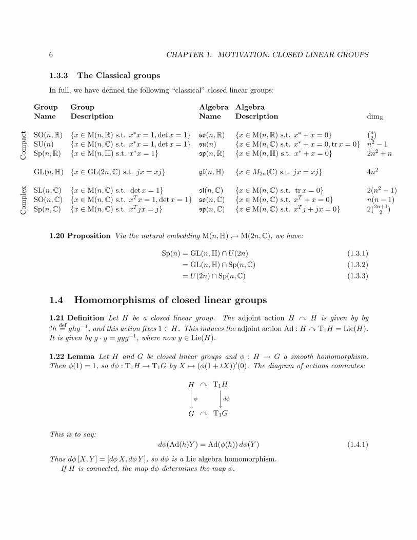
1.3.3 The Classical groups
In full, we have defined the following “classical” closed linear groups:
Group Group Algebra AlgebraName Description Name Description dimR
Com
pact SO(n,R) {x ∈ M(n,R) s.t. x∗x = 1, detx = 1} so(n,R) {x ∈ M(n,R) s.t. x∗ + x = 0}
(n2
)SU(n) {x ∈ M(n,C) s.t. x∗x = 1, detx = 1} su(n) {x ∈ M(n,C) s.t. x∗ + x = 0, trx = 0} n2 − 1Sp(n,R) {x ∈ M(n,H) s.t. x∗x = 1} sp(n,R) {x ∈ M(n,H) s.t. x∗ + x = 0} 2n2 + n
GL(n,H) {x ∈ GL(2n,C) s.t. jx = xj} gl(n,H) {x ∈M2n(C) s.t. jx = xj} 4n2
Com
plex SL(n,C) {x ∈ M(n,C) s.t. detx = 1} sl(n,C) {x ∈ M(n,C) s.t. trx = 0} 2(n2 − 1)
SO(n,C) {x ∈ M(n,C) s.t. xTx = 1,detx = 1} so(n,C) {x ∈ M(n,C) s.t. xT + x = 0} n(n− 1)Sp(n,C) {x ∈ M(n,C) s.t. xT jx = j} sp(n,C) {x ∈ M(n,C) s.t. xT j + jx = 0} 2
(2n+12
)
1.20 Proposition Via the natural embedding M(n,H) ↪→ M(2n,C), we have:
Sp(n) = GL(n,H) ∩ U(2n) (1.3.1)= GL(n,H) ∩ Sp(n,C) (1.3.2)= U(2n) ∩ Sp(n,C) (1.3.3)
1.4 Homomorphisms of closed linear groups
1.21 Definition Let H be a closed linear group. The adjoint action H y H is given by bygh
def= ghg−1, and this action fixes 1 ∈ H. This induces the adjoint action Ad : H y T1H = Lie(H).It is given by g · y = gyg−1, where now y ∈ Lie(H).
1.22 Lemma Let H and G be closed linear groups and φ : H → G a smooth homomorphism.Then φ(1) = 1, so dφ : T1H → T1G by X 7→ (φ(1 + tX))′(0). The diagram of actions commutes:
H y T1H
G y T1G
φ dφ
This is to say:dφ(Ad(h)Y ) = Ad(φ(h)) dφ(Y ) (1.4.1)
Thus dφ [X,Y ] = [dφX, dφY ], so dφ is a Lie algebra homomorphism.If H is connected, the map dφ determines the map φ.

1.4. HOMOMORPHISMS OF CLOSED LINEAR GROUPS 7
Exercises
1. (a) Show that the orthogonal groups O(n,R) and O(n,C) have two connected components,the identity component being the special orthogonal group SOn, and the other consistingof orthogonal matrices of determinant −1.
(b) Show that the center of O(n) is {±In}.(c) Show that if n is odd, then SO(n) has trivial center and O(n) ∼= SO(n) × (Z/2Z) as a
Lie group.
(d) Show that if n is even, then the center of SO(n) has two elements, and O(n) is asemidirect product (Z/2Z) n SO(n), where Z/2Z acts on SO(n) by a non-trivial outerautomorphism of order 2.
2. Construct a smooth group homomorphism Φ : SU(2)→ SO(3) which induces an isomorphismof Lie algebras and identifies SO(3) with the quotient of SU(2) by its center {±I}.
3. Construct an isomorphism of GL(n,C) (as a Lie group and an algebraic group) with a closedsubgroup of SL(n+ 1,C).
4. Show that the map C∗ × SL(n,C) → GL(n,C) given by (z, g) 7→ zg is a surjective ho-momorphism of Lie and algebraic groups, find its kernel, and describe the correspondinghomomorphism of Lie algebras.
5. Find the Lie algebra of the group U ⊆ GL(n,C) of upper-triangular matrices with 1 onthe diagonal. Show that for this group, the exponential map is a diffeomorphism of the Liealgebra onto the group.
6. A real form of a complex Lie algebra g is a real Lie subalgebra gR such that that g = gR⊕ igR,or equivalently, such that the canonical map gR⊗RC→ g given by scalar multiplication is anisomorphism. A real form of a (connected) complex closed linear group G is a (connected)closed real subgroup GR such that Lie(GR) is a real form of Lie(G).
(a) Show that U(n) is a compact real form of GL(n,C) and SU(n) is a compact real formof SL(n,C).
(b) Show that SO(n,R) is a compact real form of SO(n,C).
(c) Show that Sp(n,R) is a compact real form of Sp(n,C).
8 CHAPTER 1. MOTIVATION: CLOSED LINEAR GROUPS

Chapter 2
Mini-course in Differential Geometry
2.1 Manifolds
[8, Lectures 6, 7, and 8]
2.1.1 Classical definition
2.1 Definition Let X be a (Hausdorff) topological space. A chart consists of the data U ⊆open
X
and a homeomorphism φ : U ∼→ V ⊆open
Rn. Rn has coordinates xi, and ξidef= xi ◦ φ are local
coordinates on the chart. Charts (U, φ) and (U ′, φ′) are compatible if on U ∩ U ′ the ξ′i are smoothfunctions of the ξi and conversely. I.e.:
U ∩ U ′U U ′
φ
V
φ′
V ′
φ
W
φ′
W ′⊇V ⊆ V’φ′◦φ−1
smooth with smooth inverse
(2.1.1)
An atlas on X is a covering by pairwise compatible charts.
2.2 Lemma If U and U ′ are compatible with all charts of A, then they are compatible with eachother.
2.3 Corollary Every atlas has a unique maximal extension.
2.4 Definition A manifold is a Hausdorff topological space with a maximal atlas. It can be real,infinitely-differentiable, complex, analytic, etc., by varying the word “smooth” in the compatibilitycondition equation 2.1.1.
2.5 Definition Let U be an open subset of a manifold X. A function f : U → R is smooth if it issmooth on local coordinates in all charts.
9

10 CHAPTER 2. MINI-COURSE IN DIFFERENTIAL GEOMETRY
2.1.2 Sheafs
2.6 Definition A sheaf of functions S on a topological space X assigns a ring S (U) to each openset U ⊆
openX such that:
1. if V ⊆ U and f ∈ S (U), then f |V ∈ S (V ), and
2. if U =⋃α Uα and f : U → R such that f |Uα ∈ S (Uα) for each α, then f ∈ S (U).
The stalk of a sheaf at x ∈ X is the space Sxdef= limU3x S (U).
2.7 Lemma Let X be a manifold, and assign to each U ⊆open
X the ring C (U) of smooth functions
on U . Then C is a sheaf. Conversely, a topological space X with a sheaf of functions S is amanifold if and only if there exists a covering of X by open sets U such that (U,S |U ) is isomorphicas a space with a sheaf of functions to (V,S Rn |V ) for some V ⊆ Rn open.
2.1.3 Manifold constructions
2.8 Definition If X and Y are smooth manifolds, then a smooth map f : X → Y is a continuousmap such that for all U ⊆ Y and g ∈ C (U), then g ◦ f ∈ C (f−1(U)). Manifolds form a categoryMan with products: a product of manifolds X × Y is a manifold with charts U × V .
2.9 Definition Let M be a manifold, p ∈ M a point, and γ1, γ2 : R→ M two paths with γ1(0) =γ2(0) = p. We say that γ1 and γ2 are tangent at p if (f ◦ γ1)′(0) = (f ◦ γ2)′(0) for all smooth f ona nbhd of p, i.e. for all f ∈ Cp. Each equivalence class of tangent curves is called a tangent vector.
2.10 Definition Let M be a manifold and C its sheaf of smooth functions. A point derivation isa linear map δ : Cp → R satisfying the Leibniz rule:
δ(fg) = δf g(p) + f(p) δg (2.1.2)
2.11 Lemma Any tangent vector γ gives a point derivation δγ : f 7→ (f ◦γ)′(0). Conversely, everypoint derivation is of this form.
2.12 Lemma / Definition Let M and N be manifolds, and f : M → N a smooth map sendingp 7→ q. The following are equivalent, and define (df)p : TpM → TqN , the differential of f at p:
1. If [γ] ∈ TpM is represented by the curve γ, then (df)p(X) def= [f ◦ γ].
2. If X ∈ TpM is a point-derivation on SM,p, then (df)p(X) : SN,q → R (or C) is defined byψ 7→ X[ψ ◦ f ].
3. In coordinates, p ∈ U ⊆open
Rm and q ∈W ⊆open
Rn, then locally f is given by f1, . . . , fn smooth
functions of x1, . . . , xm. The tangent spaces to Rn are in canonical bijection with Rn, and alinear map Rm → Rn should be presented as a matrix:
Jacobian(f, x) def=∂fi∂xj
(2.1.3)

2.1. MANIFOLDS 11
2.13 Lemma We have the chain rule: if Mf→ N
g→ K, then d(g ◦ f)p = (dg)f(p) ◦ (df)p.
2.14 Theorem (Inverse Mapping Theorem) 1. Given smooth f1, . . . , fn : U → R wherep ∈ U ⊆
openRn, then f : U → Rn maps some neighborhood V 3 p bijectively to W ⊆
openRn with
s/a/h inverse iff det Jacobian(f, x) 6= 0.
2. A smooth map f : M → N of manifold restricts to an isomorphism p ∈ U → W for someneighborhood U if and only if (df)p is a linear isomorphism.
2.1.4 Submanifolds
2.15 Proposition Let M be a manifold and N a topological subspace with the induced topologysuch that for each p ∈ N , there is a chart U 3 p in M with coordinates {ξi}mi=1 : U → Rm such thatU ∩ N = {q ∈ U s.t. ξn+1(q) = · · · = ξm(q) = 0}. Then U ∩ N is a chart on N with coordinatesξ1, . . . , ξn, and N is a manifold with an atlas given by {U∩N} as U ranges over an atlas of M . Thesheaf of smooth functions CN is the sheaf of continuous functions on N that are locally restrictionsof smooth functions on M . The embedding N ↪→M is smooth, and satisfies the universal propertythat any smooth map f : Z →M such that f(Z) ⊆ N defines a smooth map Z → N .
2.16 Definition The map N ↪→ M in Proposition 2.15 is an immersed submanifold. A mapZ →M is an immersion if it factors as Z ∼→ N ↪→M for some immersed submanifold N ↪→M .
2.17 Proposition If N ↪→M is an immersed submanifold, then N is locally closed.
2.18 Proposition Any closed linear group H ⊆ GL(n) is an immersed analytic submanifold. IfLie(H) is a C-subspace of M(n,C), then H is a holomorphic submanifold.
Proof The following diagram defines a chart near 1 ∈ H, which can be moved by left-multiplicationwherever it is needed:
U Vexp
logM(n) ⊇
∈0⊆ GL(n)
∈1
Lie(H) ∩ U H ∩ V
(2.1.4)�
2.19 Lemma Given TpM = V1 ⊕ V2, there is an open neighborhood U1 × U2 of p such that Vi =TpUi.
2.20 Lemma If s : N →M ×N is a s/a/h section, then s is a (closed) immersion.
2.21 Proposition A smooth map f : N →M is an immersion on a neighborhood of p ∈ N if andonly if (df)p is injective.

12 CHAPTER 2. MINI-COURSE IN DIFFERENTIAL GEOMETRY
2.2 Vector Fields
[8, Lectures 8, 9, and 10]
2.2.1 Definition
2.22 Definition Let M be a manifold. A vector field assigns to each p ∈ M a vector xp, i.e. apoint derivation:
xp(fg) = f(p)xp(g) + xp(f) g(p) (2.2.1)
We define (xf)(p) def= xp(f). Then x(fg) = f x(g) + x(f) g, so x is a derivation. But it might bediscontinuous. A vector field x is smooth if x : CM → CM is a map of sheaves. Equivalently, inlocal coordinates the components of xp must depend smoothly on p. By changing (the conditionson) the sheaf C , we may define analytic or holomorphic vector fields.
Henceforth, the word “vector field” will always mean “smooth (or analytic or holomorphic)vector field”. Similarly, we will use the word “smooth” to mean smooth or analytic or holomorphic,depending on our category.
2.23 Lemma The commutator [x, y] def= xy − yx of derivations is a derivation.
Proof An easy calculation:
xy(fg) = xy(f) g + x(f) y(g) + y(f)x(g) + f xy(g) (2.2.2)Switch X and Y , and subtract:
[x, y](fg) = [x, y](f) g + f [x, y](g) (2.2.3)�
2.24 Definition A Lie algebra is a vector space l with a bilinear map [, ] : l × l → l (i.e. a linearmap [, ] : l⊗ l→ l), satisfying
1. Antisymmetry: [x, y] + [y, x] = 0
2. Jacobi: [x, [y, z]] + [y, [z, x]] + [z, [x, y]] = 0
2.25 Proposition Let V be a vector space. The bracket [x, y] def= xy − yx makes End(V ) into aLie algebra.
2.26 Lemma / Definition Let l be a Lie algebra. The adjoint action ad : l → End(l) given byadx : y 7→ [x, y] is a derivation:
(adx)[y, z] = [(adx)y, z] + [y, (adx)z] (2.2.4)
Moreover, ad : l→ End(l) is a Lie algebra homomorphism:
ad([x, y]) = (adx)(ad y)− (ad y)(adx) (2.2.5)
2.2. VECTOR FIELDS 13
2.2.2 Integral Curves
Let ∂t be the vector field f 7→ ddtf on R.
2.27 Proposition Given a smooth vector field x on M and a point p ∈ M , there exists an openinterval I ⊆
openR such that 0 ∈ I and a smooth curve γ : I →M satisfying:
γ(0) = p (2.2.6)(dγ)t(∂t) = xγ(t) ∀t ∈ I (2.2.7)
When M is a complex manifold and x a holomorphic vector field, we can demand that I ⊆open
C is
an open domain containing 0, and that γ : I →M be holomorphic.
Proof In local coordinates, γ : R → Rn, and we can use existence and uniqueness theorems forsolutions to differential equations; then we need that a smooth (analytic, holomorphic) differentialequation has a smooth (analytic, holomorphic) solution.
But there’s a subtlety. What if there are two charts, and solutions on each chart, that divergeright where the charts stop overlapping? Well, since M is Hausdorff, if we have two maps I →M ,then the locus where they agree is closed, so if they don’t agree on all of I, then we can go to themaximal point where they agree and look locally there. �
2.28 Definition The integral curve∫x,p(t) of x at p is the maximal curve satisfying equations 2.2.6
and 2.2.7.
2.29 Proposition The integral curve∫x,p depends smoothly on p ∈M .
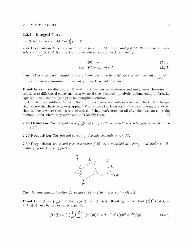
2.30 Proposition Let x and y be two vector fields on a manifold M . For p ∈ M and s, t ∈ R,define q by the following picture:
p1
p2
p3
p
q ∫x
t ∫y
s
∫x
−t
∫y
−s
Then for any smooth function f , we have f(q)− f(p) = st[x, y]pf +O(s, t)3.
Proof Let α(t) =∫x,p(t), so that f(α(t))′ = xf(α(t)). Iterating, we see that
Äddt
änf(α(t)) =
xnf(α(t)), and by Taylor series expansion,
f(α(t)) =∑ 1
n!
Åd
dt
ãnf(α(0))tn =
∑ 1n!xnf(p)tn = etxf(p). (2.2.8)

14 CHAPTER 2. MINI-COURSE IN DIFFERENTIAL GEOMETRY
By varying p, we have:
f(q) =Äe−syf
ä(p3) (2.2.9)
=Äe−txe−syf
ä(p2) (2.2.10)
=Äesye−txe−syf
ä(p1) (2.2.11)
=Äetxesye−txe−syf
ä(p) (2.2.12)
We already know that etxesye−txe−sy = 1 + st[x, y] + higher terms. Therefore f(q) − f(p) =st[x, y]pf +O(s, t)3. �
2.2.3 Group Actions
2.31 Proposition Let M be a manifold, G a Lie group, and G y M a Lie group action, i.e. asmooth map ρ : G ×M → M satisfying equations 1.1.5 and 1.1.6. Let x ∈ TeG, where e is theidentity element of the group G. The following descriptions of a vector field `x ∈ Vect(M) areequivalent:
1. Let x = [γ] be the equivalence class of tangent paths, and let γ : I → G be a representativepath. Define (`x)m = [γ] where γ(t) def= ρ
Äγ(t)−1,m
ä. On functions, `x acts as:
(`x)mfdef=
d
dt
∣∣∣∣t=0
fÄγ(t)−1m
ä(2.2.13)
2. Arbitrarily extend x to a vector field x on a neighborhood U ⊆ G of e, and lift this to ˜x onU ×M to point only in the U -direction: ˜x(u,m)
def= (xu, 0) ∈ TuU × TmM . Let `x act onfunctions by:
(`x)f def= −˜x(f ◦ p)∣∣∣{e}×M=M
(2.2.14)
3. (`x)mdef= −(dρ)(e,m)(x, 0)
2.32 Proposition Let G be a Lie group, M and N manifolds, and GyM , Gy N Lie actions,and let f : M → N be G-equivariant. Given x ∈ TeG, define `Mx and `Nx vector fields on M andN as in Proposition 2.31. Then for each m ∈M , we have:
(df)m(`Mx) = (`Nx)f(m) (2.2.15)
2.33 Definition Let G y M be a Lie action. We define the adjoint action of G on Vect(M) bygy
def= dg(y)gm = (dg)m(ym). Equivalently, G y CM by g : f 7→ f ◦ g−1, and given a vector field
thought of as a derivation y : CM → CM , we define gydef= gyg−1.
2.34 Example Let G y G by right multiplication: ρ(g, h) def= hg−1. Then G y TeG by theadjoint action Ad(g) = d(g − g−1)e, i.e. if x = [γ], then Ad(g)x = [g γ(t) g−1].

2.2. VECTOR FIELDS 15
2.35 Definition Let ρ : GyM be a Lie action. For each g ∈ G, we define gM to be the manifoldM with the action gρ : (h,m) 7→ ρ(ghg−1,m).
2.36 Corollary For each g ∈ G, the map g : M → gM is G-equivariant. We have:
g`x = dg(`x) = `gMx = `(Ad(g)x) (2.2.16)
2.37 Proposition Let ρ : Gy G by ρg : h 7→ hg−1. Then ` : TeG→ Vect(G) is an isomorphismfrom TeG to left-invariant vector fields, such that (`x)e = x.
Proof Let λ : G y G be the action by left-multiplication: λg(h) = gh. Then for each g, λg is ρ-equivariant. Thus dλg(`x) = λg(`x) = `x, so `x is left-invariant, and (`x)e = x since ρ(g, e) = g−1.Conversely, a left-invariant field is determined by its value at a point:
(`x)g = (dλg)e(`xe) = (dλg)e(x) (2.2.17)�
2.2.4 Lie algebra of a Lie group
2.38 Lemma / Definition Let GyM be a Lie action. The subspace of Vect(M) of G-invariantderivations is a Lie subalgebra of Vect(M).
Let G be a Lie group. The Lie algebra of G is the Lie subalgebra Lie(G) of Vect(G) consistingof left-invariant vector fields, i.e. vector fields invariant under the action λ : G y G given byλg : h 7→ gh.
We identify Lie(G) def= TeG as in Proposition 2.37.
2.39 Lemma Given G y M a Lie action, x ∈ Lie(G) represented by x = [γ], and y ∈ Vect(M),we have:
d
dt
∣∣∣∣t=0
γ(t)yf = [`x, y]f (2.2.18)
Proof
d
dt
∣∣∣∣t=0
γ(t)yf (p) =d
dt
∣∣∣∣t=0
γ(t) y γ(t)−1f (p) (2.2.19)
=d
dt
∣∣∣∣t=0
γ(t) y f(γ(t) p) (2.2.20)
=d
dt
∣∣∣∣t=0
γ(t) y f(γ(0) p) + γ(0)d
dt
∣∣∣∣t=0
yf(γ(t)p) (2.2.21)
= `x(yf)(p) + yd
dt
∣∣∣∣t=0
f(γ(t)p) (2.2.22)
= `x(yf)(p) + y(−`x f)(p) (2.2.23)= [`x, y]f (p) (2.2.24)
�

16 CHAPTER 2. MINI-COURSE IN DIFFERENTIAL GEOMETRY
2.40 Corollary Let GyM be a Lie action. If x, y ∈ Lie(G), where x = [γ], then
`MÄ`Ad(−x) y
ä=
d
dt
∣∣∣∣t=0
`ÄAd(γ(t))y
äf = [`x, `y] f (2.2.25)
2.41 Lemma The Lie bracket defined on Lie(GL(n)) = gl(n) = Te GL(n) = M(n) defined inLemma/Definition 2.38 is the matrix bracket [x, y] = xy − yx.
Proof We represent x ∈ gl(n) by [etx]. The adjoint action on GL(n) is given by AdG(g)h = ghg−1,which is linear in h and fixes e, and so passes immediately to the action Ad : GL(n) y Te GL(n)given by Adg(g) y = gyg−1. Then
[x, y] =d
dt
∣∣∣∣t=0
etxye−tx = xy − yx. (2.2.26)�
2.42 Corollary If H is a closed linear group, then Lemma/Definitions 2.38 and 1.7 agree.
Exercises
1. (a) Show that the composition of two immersions is an immersion.(b) Show that an immersed submanifold N ⊆M is always a closed submanifold of an open
submanifold, but not necessarily an open submanifold of a closed submanifold.
2. Prove that if f : N → M is a smooth map, then (df)p is surjective if and only if there areopen neighborhoods U of p and V of f(p), and an isomorphism ψ : V ×W → U , such thatf ◦ ψ is the projection on V .
In particular, deduce that the fibers of f meet a neighborhood of p in immersed closedsubmanifolds of that neighborhood.
3. Prove the implicit function theorem: a map (of sets) f : M → N between manifolds is smoothif and only if its graph is an immersed closed submanifold of M ×N .
4. Prove that the curve y2 = x3 in R2 is not an immersed submanifold.
5. Let M be a complex holomorphic manifold, p a point of M , X a holomorphic vector field.Show that X has a complex integral curve γ defined on an open neighborhood U of 0 inC, and unique on U if U is connected, which satisfies the usual defining equation but in acomplex instead of a real variable t.
Show that the restriction of γ to U ∩ R is a real integral curve of X, when M is regarded asa real analytic manifold.
6. Let SL(2,C) act on the Riemann sphere P1(C) by fractional linear transformationsña bc d
ôz =
(az+ b)/(cz+ d). Determine explicitly the vector fields f(z)dz corresponding to the infinites-imal action of the basis elements
E =ñ
0 10 0
ô, H =
ñ1 00 −1
ô, F =
ñ0 01 0
ô

2.2. VECTOR FIELDS 17
of sl(2,C), and check that you have constructed a Lie algebra homomorphism by computingthe commutators of these vector fields.
7. (a) Describe the map gl(n,R) = Lie(GL(n,R)) = M(n,R) → Vect(Rn) given by the in-finitesimal action of GL(n,R).
(b) Show that so(n,R) is equal to the subalgebra of gl(n,R) consisting of elements whoseinfinitesimal action is a vector field tangential to the unit sphere in Rn.
8. (a) Let X be an analytic vector field on M all of whose integral curves are unbounded (i.e.,they are defined on all of R). Show that there exists an analytic action of R = (R,+)on M such that X is the infinitesimal action of the generator ∂t of Lie(R).
(b) More generally, prove the corresponding result for a family of n commuting vector fieldsXi and action of Rn.
9. (a) Show that the matrixñ−a 00 −b
ôbelongs to the identity component of GL(2,R) for all
positive real numbers a, b.
(b) Prove that if a 6= b, the above matrix is not in the image exp(gl(2,R)) of the exponentialmap.

18 CHAPTER 2. MINI-COURSE IN DIFFERENTIAL GEOMETRY

Chapter 3
General theory of Lie groups
3.1 From Lie algebra to Lie group
3.1.1 The exponential map
[8, Lecture 10]We state the following results for Lie groups over R. When working with complex manifolds,
we can replace R by C throughout, whence the interval I ⊆open
R is replaced by a connected open
domain I ⊆open
C. As always, the word “smooth” may mean “infinitely differentiable” or “analytic”or . . . .
3.1 Lemma Let G be a Lie group and x ∈ Lie(G). Then there exists a unique Lie group homo-morphism γx : R→ G such that (dγx)0(∂t) = x. It is given by γx(t) = (
∫e `x)(t).
Proof Let γ : I → G be the maximal integral curve of `x passing through e. Since `x is left-invariant, gγ(t) is an integral curve through q. Let g = γ(s) for s ∈ I; then γ(t) and γ(s)γ(t)are integral curves through γ(s), to they must coincide: γ(s + t) = γ(s)γ(t), and γ(−s) = γ(s)−1
for s ∈ I ∩ (−I). So γ is a groupoid homomorphism, and by defining γ(s + t) def= γ(s)γ(t) fors, t ∈ I, s+ t 6∈ I, we extend γ to I + I. Since R is archimedean, this allows us to extend γ to allof R; it will continue to be an integral curve, so really I must have been R all along. �
3.2 Corollary There is a bijection between one-parameter subgroups of G (homomorphisms R→G) and elements of the Lie algebra of G.
3.3 Definition The exponential map exp : Lie(G)→ G is given by expx def= γx(1), where γx is asin Lemma 3.1.
3.4 Proposition Let x(b) be a smooth family of vector fields on M parameterized by b ∈ B amanifold, i.e. the vector field x on B ×M given by x(b,m) = (0, x(b)
m ) is smooth. Then (b, p, t) 7→Ä∫p x
(b)ä
(t) is a smooth map from an open neighborhood of B×M×{0} in B×M×R to M . Wheneach x(b) has infinite-time solutions, we can take the open neighborhood to be all of B ×M × R.
19

20 CHAPTER 3. GENERAL THEORY OF LIE GROUPS
Proof Note that Ç∫(b,p)
x
å(t) =
Çb,
Ç∫px(b)
å(t)å
(3.1.1)
So B×M ×R→ B×M π→M by (b, p, t) 7→Ä∫
(b,p) xä
(t) 7→Ä∫p x
(b)ä
(t) is a composition of smoothfunctions, hence is smooth. �
3.5 Theorem (Exponential Map) For each Lie group G, there is a unique smooth map exp :Lie(G) → G such that for x ∈ Lie(G), the map t 7→ exp(tx) is the integral curve of `x through e;t 7→ exp(tx) is a Lie group homomorphism R→ G.
3.6 Example When G = GL(n), the map exp : gl(n)→ GL(n) is the matrix exponential.
3.7 Proposition The differential at the origin (d exp)0 is the identity map 1Lie(G).
Proof d(exp tx)0(∂t) = x. �
3.8 Corollary exp is a local homeomorphism.
3.9 Definition The local inverse of exp : Lie(G)→ G is called “log”.
3.10 Proposition If G is connected, then exp(Lie(G)) generates G.
3.11 Proposition If φ : H → G is a group homomorphism, then the following diagram commutes:
Lie(H)
H
Lie(G)
G
exp exp
(dφ)e
φ
(3.1.2)
If H is connected, then dφ determines φ.
3.1.2 The Fundamental Theorem
[8, Lecture 11]Like all good algebraists, we assume that Axiom of Choice.
3.12 Theorem (Fundamental Theorem of Lie Groups and Algebras)
1. The functor G 7→ Lie(G) gives an equivalence of categories between the category scLieGp ofsimply-connected Lie groups (over R or C) and the category LieAlg of finite-dimensionalLie algebras (over R or C).
2. “The” inverse functor h 7→ Grp(h) is left-adjoint to Lie : LieAlg→ LieGp.

3.1. FROM LIE ALGEBRA TO LIE GROUP 21
We outline the proof. Consider open neighborhood U and V so that the horizontal maps are ahomeomorphism:
U V
⊆
Lie(G)
⊆
G
∈
0
∈
e
exp
log(3.1.3)
Consider the restriction µ : G×G→ G to (V ×V )∩µ−1(V )→ V , and use this to define a “partialgroup law” b : open→ U , where open ⊆ U × U , via
b(x, y) def= log(expx exp y) (3.1.4)
We will show that the Lie algebra structure of Lie(G) determines b.Moreover, given h a finite-dimensional Lie algebra, we will need to define b and build H as the
group freely generated by U modulo the relations xy = b(x, y) if x, y, b(x, y) ∈ U . We will need toprove that H is a Lie group, with U as an open submanifold.
3.13 Corollary Every Lie subalgebra h of Lie(G) is Lie(H) for a unique connected subgroup H ↪→G, up to equivalence.
The standard proof of Theorem 3.12 is to first prove Corollary 3.13 and then use Theorem 4.99.We will use Theorem 4.89 rather than Theorem 4.99.
3.14 Theorem (Baker-Campbell-Hausdorff Formula (second part only))
1. Let T (x, y) be the free tensor algebra generated by x and y, and T (x, y)[[s, t]] the (non-commutative) ring of formal power series in two commuting variables s and t. Define b(tx, sy) def=log(exp(tx) exp(sy)) ∈ T (x, y)[[s, t]], where exp and log are the usual formal power series.Then
b(tx, sy) = tx+ sy + st12
[x, y] + st2112
[x, [x, y]] + s2t112
[y, [y, x]] + . . . (3.1.5)
has coefficients all coefficients given by Lie bracket polynomials in x and y.
2. Given a Lie group G, there exists a neighborhood U ′ 3 0 in Lie(G) such that U ′ ⊆ Uexp
�log
V ⊆ G
and b(x, y) converges on U ′ × U ′ to log(expx exp y).
We need more machinery than we have developed so far to prove part 1. We work with analyticmanifolds; on C manifolds, we can make an analogous argument using the language of differentialequations.
Proof (of part 2.) For a clearer exposition, we distinguish the maps exp : Lie(G) → G fromex ∈ R[[x]].
22 CHAPTER 3. GENERAL THEORY OF LIE GROUPS
We begin with a basic identity. exp(tx) is an integral curve to `x through e, so by left-invariance,t 7→ g exp(tx) is the integral curve of `x through g. Thus, for f analytic on G,
d
dt
îf(g exp tx)
ó=Ä(`x)f
ä(g exp tx) (3.1.6)
We iterate: Åd
dt
ãn îf(g exp tx)
ó=Ä(`x)nf
ä(g exp tx) (3.1.7)
If f is analytic, then for small t the Taylor series converges:
f(g exp tx) =∞∑n=0
Åd
dt
ãn îf(g exp tx)
ó∣∣∣∣t=0
tn
n!(3.1.8)
=∞∑n=0
Ä(`x)nf
ä(g exp tx)
∣∣∣t=0
tn
n!(3.1.9)
=∞∑n=0
Ä(`x)nf
ä(g)
tn
n!(3.1.10)
=∞∑n=0
Ç(t `x)n
n!f
å(g) (3.1.11)
=Äet `xf
ä(g) (3.1.12)
We repeat the trick:
f(exp tx exp sy) =ÄesLyf
ä(exp tx) =
Äet `xesLyf
ä(e) =
Äetxesyf
ä(e) (3.1.13)
The last equality is because we are evaluating the derivations at e, where `x = x.We now let f = log : V → U , or rather a coordinate of log. Then the left-hand-side is just
log(exp tx exp sy), and the right hand side isÄetxesy log
ä(e) =
Äeb(tx,sy) log
ä(e), where b is the formal
power series from part 1. — we have shown that the right hand side converges. But by interpretingthe calculations above as formal power series, and expanding log in Taylor series, we see that theformal power series
Äeb(tx,sy) log
ä(e) agrees with the formal power series log
Äeb(tx,sy)
ä= b(tx, sy).
This completes the proof of part 2. �
3.2 Universal Enveloping Algebras
3.2.1 The Definition
[8, Lecture 12]
3.15 Definition A representation of a Lie group is a homomorphism G → GL(n,R) (or C). Arepresentation of a Lie algebra is a homomorphism Lie(G) → gl(n) = End(V ); the space End(V )is a Lie algebra with the bracket given by [x, y] = xy − yx.
3.2. UNIVERSAL ENVELOPING ALGEBRAS 23
3.16 Definition Let V be a vector space. The tensor algebra over V is the free unital non-commuting algebra T V generated by a basis of V . Equivalently:
T V def=⊕n≥0
V ⊗n (3.2.1)
The multiplication is given by ⊗ : V ⊗k × V ⊗l → V ⊗(k+l). T is a functor, and is left-adjoint toForget : Alg→ Vect.
3.17 Definition Let g be a Lie algebra. The universal enveloping algebra is
Ugdef= T g/
¨[x, y]− (xy − yx)
∂(3.2.2)
U : LieAlg→ Alg is a functor, and is left-adjoint to Forget : Alg→ LieAlg.
3.18 Corollary The category of g-modules is equal to the category of Ug-modules.
3.19 Example A Lie algebra g is abelian if the bracket is identically 0. If g is abelian, thenUg = Sg, where SV is the symmetric algebra generated by the vector space V (so that S isleft-adjoint to Forget : ComAlg→ Vect).
3.20 Example If f is the free Lie algebra on generators x1, . . . , xd, defined in terms of a universalproperty, then U f = T (x1, . . . , xd).
3.21 Definition A vector space V is graded if it comes with a direct-sum decomposition V =⊕n≥0 Vn. A morphism of graded vector spaces preserves the grading. A graded algebra is an
algebra object in the category of graded vector spaces. I.e. it is a vector space V =⊕
n≥0 alongwith a unital associative multiplication V ⊗ V → V such that if vn ∈ Vn and vm ∈ Vm, thenvnvm ∈ Vn+m.
A vector space V is filtered if it comes with an increasing sequence of subspaces
{0} ⊆ V≤0 ⊆ V≤1 ⊆ · · · ⊆ V (3.2.3)
such that V =⋃n≥0 Vn. A morphism of graded vector spaces preserves the filtration. A filtered
algebra is an algebra object in the category of filtered vector spaces. I.e. it is a filtered vector spacealong with a unital associative multiplication V ⊗ V → V such that if vn ∈ V≤n and vm ∈ V≤m,then vnvm ∈ V≤(n+m).
Given a filtered vector space V , we define grV def=⊕n≥0 grn V , where grn V
def= V≤n/V≤(n−1).
3.22 Lemma gr is a functor. If V is a filtered algebra, then grV is a graded algebra.
3.23 Example Let g be a Lie algebra over K. Then Ug has a natural filtration inherited from thefiltration of T g, since the ideal 〈xy − yx = [x, y]〉 preserves the filtration. Since Ug is generatedby g, so is grUg; since xy − yx = [x, y] ∈ U≤1, grUg is commutative, and so there is a naturalprojection Sg� grUg.

24 CHAPTER 3. GENERAL THEORY OF LIE GROUPS
3.2.2 Poincare-Birkhoff-Witt Theorem
[8, Lectures 12 and 13]
3.24 Theorem (Poincare-Birkhoff-Witt) The map Sg→ grUg is an isomorphism of algebras.
3.25 Corollary g ↪→ Ug. Thus every Lie algebra is isomorphic to a Lie subalgebra of someEnd(V ), namely V = Ug.
Proof (of Theorem 3.24) Pick an ordered basis {xα} of g; then the monomials xα1 . . . xαn forα1 ≤ · · · ≤ αn are an ordered basis of Sg, where we take the “deg-lex” ordering: a monomial of lowerdegree is immediately smaller than a monomial of high degree, and for monomials of the same degreewe alphabetize. Since Sg� grUg is an algebra homomorphism, the set {xα1 . . . xαn s.t. α1 ≤ · · · ≤αn} spans grUg. It suffices to show that they are independent in grUg. For this it suffices to showthat the set S def= {xα1 . . . xαn s.t. α1 ≤ · · · ≤ αn} is independent in Ug.
Let I = 〈xy − yx − [x, y]〉 be the ideal of T g such that Ug = T g/I. Define J ⊆ T g to be thespan of expressions of the form
ξ = xα1 · · ·xαk (xβxγ − xγxβ − [xβ, xγ ])xν1 · · ·xνl (3.2.4)
where α1 ≤ · · · ≤ αk ≤ β > γ, and there are no conditions on νi, so that J is a right ideal. Wetake the deg-lex ordering in T g. The leading monomial in equation 3.2.4 is x~αxβxγx~ν . Thus S isan independent set in T g/J . We need only show that J = I.
The ideal I is generated by expressions of the form xβxγ − xγxβ − [xβ, xγ ] as a two-sided ideal.If β > γ then
Äxβxγ − xγxβ − [xβ, xγ ]
ä∈ J ; by antisymmetry, if β < γ we switch them and stay
in J . If β = γ, thenÄxβxγ − xγxβ − [xβ, xγ ]
ä= 0. Thus J is a right ideal contained in I, and the
two-sided ideal generated by J contains I. Thus the two-sided ideal generated by J is I, and itsuffices to show that J is a two-sided ideal.
We multiply xδξ. If k > 0 and δ ≤ α1, then xδξ ∈ J . If δ > α1, then xδξ ≡ xα1xδxα2 · · · +[xδ, xα1 ]xα2 . . . mod J . And both xδxα2 . . . and [xδ, xα1 ]xα2 . . . are in J by induction on degree.Then since α1 < δ, xα1xδxα2 · · · ∈ J by (transfinite) induction on δ.
So suffice to show that if k = 0, then we’re still in J . I.e. if α > β > γ, then we want to showthat xα (xβxγ − xγxβ − [xβ, xγ ]) ∈ J . Well, since α > β, we see that xαxβ − xβ − [xα, xβ] ∈ J , andsame with β ↔ γ. So, working modulo J , we have
xα (xβxγ − xγxβ − [xβ, xγ ]) ≡ (xβxα + [xα, xβ])xγ − (xγxα + [xα, xγ ])xβ − xα[xβ, xγ ]≡ xβ (xγxα + [xα, xγ ]) + [xα, xβ]xγ − xγ (xβxα + [xα, xβ])− [xα, xγ ]xβ − xα[xβ, xγ ]
≡ xγxβxα + [xβ, xγ ]xα + xβ[xα, xγ ] + [xα, xβ]xγ − xγ (xβxα + [xα, xβ])− [xα, xγ ]xβ − xα[xβ, xγ ]
= [xβ, xγ ]xα + xβ[xα, xγ ] + [xα, xβ]xγ − xγ [xα, xβ]− [xα, xγ ]xβ − xα[xβ, xγ ]≡ −[xα, [xβ, xγ ]] + [xβ, [xα, xγ ]]− [xγ , [xα, xβ]]= 0 by Jacobi. �

3.2. UNIVERSAL ENVELOPING ALGEBRAS 25
3.2.3 Ug is a bialgebra
[8, Lecture 13]
3.26 Definition An algebra over K is a vector space U along with a K-linear “multiplication”map µ : U ⊗
KU → U which is associative, i.e. the following diagram commutes:
U ⊗ U ⊗ U U ⊗ U
U ⊗ U U
1U⊗µ
µ⊗1U µ
µ
(3.2.5)
We demand that all our algebras be unital, meaning that there is a linear map e : K→ U such thatthe maps U = K ⊗ U e⊗1U→ U ⊗ U µ→ U and U = U ⊗K 1U⊗e→ U ⊗ U µ→ U are the identity maps.We will call the image of 1 ∈ K under e simply 1 ∈ U .
A coalgebra is an algebra in the opposite category. I.e. it is a vector space U along with a“comultiplication” map ∆ : U → U ⊗ U so that the following commutes:
U U ⊗ U
U ⊗ U U ⊗ U ⊗ U
∆
∆ 1U⊗∆
∆⊗1U
(3.2.6)
In elements, if ∆x =∑x(1) ⊗ x(2), then we demand that
∑x(1) ⊗∆(x(2)) =
∑∆(x(1))⊗ x(1). We
demand that our coalgebras be counital, meaning that there is a linear map ε : U → K such that
the maps U ∆→ U ⊗ Uε⊗1UK ⊗ U = U and U ∆→ U ⊗ U
1U⊗εU ⊗K = U are the identity maps.
A bialgebra is an algebra in the category of coalgebras, or equivalently a coalgebra in the categoryof algebras. I.e. it is a vector space U with maps µ : U ⊗ U → U and ∆ : U → U ⊗ U satisfyingequations 3.2.5 and 3.2.6 such that ∆ and ε are (unital) algebra homomorphisms or equivalently suchthat µ and e are (counital) coalgebra homomorphism. We have defined the multiplication on U ⊗Uby (x⊗y)(z⊗w) = (xz)⊗(yw), and the comultiplication by ∆(x⊗y) =
∑∑x(1)⊗y(1)⊗x(2)⊗y(2),
where ∆x =∑x(1) ⊗ x(2) and ∆y =
∑y(1) ⊗ y(2); the unit and counit are e⊗ e and ε⊗ ε.
3.27 Definition Let U be a bialgebra, and x ∈ U . We say that x is primitive if ∆x = x⊗1+1⊗x,and that x is grouplike if ∆x = x⊗ x. The set of primitive elements of U we denote by primU .
3.28 Proposition Ug is a bialgebra with primUg = g.
Proof To define the comultiplication, it suffices to show that ∆ : g → Ug ⊗ Ug given by x 7→x⊗1+1⊗x is a Lie algebra homomorphism, whence it uniquely extends to an algebra homomorphism

26 CHAPTER 3. GENERAL THEORY OF LIE GROUPS
by the universal property. We compute:
[x⊗ 1 + 1⊗ x, y ⊗ 1 + 1⊗ y]U⊗U = [x⊗ 1, y ⊗ 1] + [1⊗ x, 1⊗ y] (3.2.7)= [x, y]⊗ 1 + 1⊗ [x, y] (3.2.8)
To show that ∆ thus defined is coassiciative, it suffices to check on the generating set g, where wesee that ∆2(x) = x⊗ 1⊗ 1 + 1⊗ x⊗ 1 + 1⊗ 1⊗ x.
By definition, g ⊆ Ug. To show equality, we use Theorem 3.24. We filter Ug⊗Ug in the obviousway, and since ∆ is an algebra homomorphism, we see that ∆
ÄUg≤1
ä⊆ÄUg ⊗ Ug
ä≤1
, whence
∆ÄUg≤n
ä⊆ÄUg ⊗ Ug
ä≤n. Thus ∆ induces a map ∆ on grUg = Sg, and ∆ makes Sg into a
bialgebra.Let ξ ∈ Ug≤n be primitive, and define its image to be ξ ∈ grn Ug; then ξ must also be primitive.
But Sg⊗ Sg = K[yα, zα], where {xα} is a basis of g (whence Sg = K[xα]), and we set yα = xα ⊗ 1and zα = 1⊗xα]. We check that ∆(xα) = yα+zα, and so if f(x) ∈ Sg, we see that ∆f(x) = f(y+z).So f ∈ Sg is primitive if and only if f(y + z) = f(y) + f(z), i.e. iff f is homogenoues of degree 1.Therefore prim grUg = gr1 Ug, and so if ξ ∈ Ug is primitive, then ξ ∈ gr1 Ug so ξ = x+ c for somex ∈ g and some c ∈ K. Since x is primitive, c must be also, and the only primitive constant is 0.�
3.2.4 Geometry of the Universal Enveloping Algebra
[8, Lecture 14]
3.29 Definition Let X be a space and S a sheaf of functions on X. We define the sheaf D ofgrothendieck differential operators inductively. Given U ⊆
openX, we define D≤0(U) = S (U), and
D≤n(U) = {x : S (U) → S (U) s.t. [x, f ] ∈ D≤(n−1)(U) ∀f ∈ S (U)}, where S (U) y S (U) byleft-multiplication. Then D(U) =
⋃n≥0 D≤n(U) is a filtered sheaf; we say that x ∈ D≤n(U) is an
“nth-order differential operator on U”.
3.30 Lemma D is a sheaf of filtered algebras, with the multiplication on D(U) inherited fromEnd(S (U)). For each n, D≤n is a sheaf of Lie subalgebras of D .
3.31 Theorem (Grothendieck Differential Operators) Let X be a manifold, C the sheaf ofsmooth functions on X, and D the sheaf of differential operators on C as in Definition 3.29. ThenD(U) is generated as a noncommutative algebra by C (U) and Vect(U), and D≤1 = C (U)⊕Vect(U).
3.32 Proposition Let G be a Lie group, and D(G)G the subalgebra of left-invariant differentialoperators on G. The natural map Ug → D(G)G generated by the identification of g with left-invariant vector fields is an isomorphism of algebras.
3.3 The Baker-Campbell-Hausdorff Formula
[8, Lecture 14]

3.3. THE BAKER-CAMPBELL-HAUSDORFF FORMULA 27
3.33 Lemma Let U be a bialgebra with comultiplication ∆. Define ∆ : U [[s]] → (U ⊗ U)[[s]] bylinearity; then ∆ is an s-adic-continuous algebra homomorphism, and so commutes with formalpower series.
Let ψ ∈ U [[s]] with ψ(0) = 0. Then ψ is primitive term-by-term — ∆(ψ) = ψ ⊗ 1 + 1 ⊗ ψ,if and only if eψ is “group-like” in the sense that ∆(eψ) = eψ ⊗ eψ, where we have defined ⊗ :U [[s]]⊗ U [[s]]→ (U ⊗ U)[[s]] by sn ⊗ sm 7→ sn+m.
Proof eψ ⊗ eψ = (1⊗ eψ)(eψ ⊗ 1) = e1⊗ψeψ⊗1 = e1⊗ψ+ψ⊗1 �
3.34 Lemma Let G be a Lie group, g = Lie(G), and identify Ug with the left-invariant differentialoperators on G, as in Proposition 3.32. Let C (G)e be the stalk of smooth functions defined in someopen set around e (we write C for the sheaf of functions on G; when G is analytic, we really meanthe sheaf of analytic functions on G). Then if u ∈ Ug satisfied uf(e) = 0 for each f ∈ C (G)e, thenu = 0.
Proof For g ∈ G, we have uf(g) = u(λg−1f)(e) = λg−1(uf)(e) = 0. �
3.35 Theorem (Baker-Campbell-Hausdorff Formula) 1. Let f be the free Lie algebra ontwo generators x, y; recall that U f = T (x, y). Define the formal power series b(tx, sy) ∈T (x, y)[[s, t]], where s and t are commuting variables, by
eb(tx,sy) def= etxesy (3.3.1)
Then b(tx, sy) ∈ f[[s, t]], i.e. b is a series all of whose coefficients are Lie algebra polynomialsin the generators x and y.
2. If G is a Lie group (in the analytic category), then there are open neighborhoods 0 ∈ U ′ ⊆open
U ⊆open
Lie(G) = g and 0 ∈ V ′ ⊆open
V ⊆open
G such that Uexp
�log
V and U ′ � V ′ and such that
b(x, y) converges on U ′ × U ′ to log(expx exp y).
Proof 1. Let ∆ : T (x, y)[[s, t]] = U f[[s, t]] → (U f ⊗ U f)[[s, t]] as in Lemma 3.33. Since etxesy isgrouplike —
∆(etxesy) = ∆(etx) ∆(esy) =Äetx ⊗ etx
ä(esy ⊗ esy) = etxesy ⊗ etxety (3.3.2)
— we see that b(tx, sy) is primitive term-by-term.
2. Let U, V be open neighborhoods of Lie(G) and G respectively, and pick V ′ so that µ : G×G→G restricts to a map V ′ × V ′ → V ; let U ′ = log(V ′). Define β(x, y) = log(expx exp y); thenβ is an analytic function U ′ × U ′ → U ′.
Let x, y ∈ Lie(G) and f ∈ C (G)e. ThenÄetxesyf
ä(e) is the Taylor series expansion of
f(exp tx exp sy), as in the proof of Theorem 3.14. Let β be the formal power series that is theTaylor expansion of β; then eβ(tx,sy)f(e) is also the Taylor series expansion of f(exp tx exp sy).This implies that for every f ∈ C (G)e, eβ(tx,sy)f(e) and etxesyf(e) have the same coefficients.

28 CHAPTER 3. GENERAL THEORY OF LIE GROUPS
But the coefficients are left-invariant differential operators applied to f , so by Lemma 3.34the series eβ(tx,sy) and etxesy must agree. Upon applying the formal logarithms, we see thatb(tx, sy) = β(tx, sy).
But β is the Taylor series of the analytic function β, so by shrinking U ′ (and hence V ′) wecan assure that it converges. �
3.4 Lie Subgroups
3.4.1 Relationship between Lie subgroups and Lie subalgebras
[8, Lecture 15]
3.36 Definition Let G be a Lie group. A Lie subgroup of G is a subgroup H of G with its ownLie group structure, so that the inclusion H ↪→ G is a local immersion. We will write “H ≤ G”when H is a Lie subgroup of G.
3.37 Theorem (Identification of Lie subalgebras and Lie subgroups) Every Lie subalgebraof Lie(G) is Lie(H) for a unique connected Lie subgroup H ≤ G.
Proof We first prove uniqueness. If H is a Lie subgroup of G, with h = Lie(H) and g = Lie(G),then the following diagram commutes:
h g
H Gexp exp (3.4.1)
This shows that expG(h) ⊆ H, and so expG(h) = expH(h), and if H is connected, this generates H.So H is uniquely determined by h as a group. Its manifold structure is also uniquely determined:we pick U, V so that the vertical arrows are an isomorphism:
0 ∈ U ⊆ g
e ∈ V ⊆ Gexp log (3.4.2)
Then exp(U ∩ h) ∼→log
U ∩ h is an immersion into g, and this defines a chart around e ∈ H, which
we can push to any other point h ∈ H by multiplication by h. This determines the topology andmanifold structure of H.
We turn now to the question of existence. We pick U and V as in equation 3.4.2, and thenchoose V ′ ⊆
openV and U ′
def= log V ′ such that:
1. (V ′)2 ⊆ V and (V ′)−1 = V ′
2. b(x, y) converges on U ′ × U ′ to log(expx exp y)

3.4. LIE SUBGROUPS 29
3. hV ′h−1 ⊆ V for h ∈ V ′
4. eadxy converges on U ′ × U ′ to logÄ(expx)(exp y)(expx)−1
ä5. b(x, y) and eadxy are elements of h ∩ U for x, y ∈ h ∩ U ′
Each condition can be independently achieved on a small enough open set. In condition 4., weconsider extend the formal power series et to operators, and remark that in a neighborhood of0 ∈ g, if h = expx, then Adh = eadx. Moreover, the following square always commutes:
g g
G Gexp exp
Ad(h)
g 7→hgh−1
(3.4.3)
Thus, we define W = exp(h ∩ U ′), which is certainly an immersed submanifold of G, as h ∩ U ′ isan open subset of the immersed submanifold h ↪→ g. We define H to be the subgroup generatedby W . Then H and W satisfy the hypotheses of Proposition 3.38. �
3.38 Proposition We use the word “manifold” to mean “object in a particular chosen categoryof sheaves of functions”. We use the word “smooth” to mean “morphism in this category”.
Let H be a group and U ⊆ H such that e ∈ U and U has the structure of a manifold. Assumefurther that the maps U × U → H, −1 : U → H, and (for each h in a generating set of H)Ad(h) : U → H mapping u 7→ huh−1 have the following properties:
1. The preimage of U ⊆ H under each map is open in the domain.
2. The restriction of the map to this preimage is smooth.
Then H has a unique structure as a group manifold such that U is an open submanifold.
Proof The conditions 1. and 2. are preserved under compositions, so Ad(x) satisfies both conditionsfor any x ∈ H. Let e ∈ U ′ ⊆
openU so that (U ′)3 ⊆ U and (U ′)−1 = U ′.
For x ∈ H, view each coset xU ′ as a manifold via U ′ x·→ xU ′. For any U ′′ ⊆open
U ′ and x, y ∈ G,
consider yU ′′∩xU ′; as a subset of xU ′, it is isomorphic to x−1yU ′′∩U ′. If this set is empty, then itis open. Otherwise, x−1yu2 = u1 for some u2 ∈ U ′′ and u1 ∈ U ′, so y−1x = u2u
−11 ∈ (U ′)2 and so
y−1xU ′ ⊆ U . In particular, the {y−1x}×U ′ ⊆ µ−1(U)∩(U×U). By the assumptions, U ′ → y−1xUis smooth, and so x−1yU ′′∩U ′, the preimage of U ′′, is open in U ′. Thus the topologies and smoothstructures on xU ′ and yU ′ agree on their overlap.
In this way, we can put a manifold structure on H by declaring that S ⊆open
H if S∩xU ′ ⊆open
xU ′
for all x ∈ H — the topology is locally the topology of U 3 e, and so is Hausdorff — , and that afunction f on S ⊆
openH is smooth if its restriction to each S ∩ xU ′ is smooth.
If we were to repeat this story with right cosets rather than left cosets we would get the a similarstructure: all the left cosets xU ′ are compatible, an all the right cosets U ′x are compatible. To

30 CHAPTER 3. GENERAL THEORY OF LIE GROUPS
show that a right coset is compatible with a left coset, it suffices to show that for each x ∈ H, xU ′
and U ′x have compatible smooth structures. We consider xU ′ ∩U ′x ⊆ xU ′, which we transport toU ′ ∩ x−1U ′x ⊆ U ′. Since we assumed that conjugation by x was a smooth map, we see that rightand left cosets are compatible.
We now need only check that the group structure is by smooth maps. We see that (xU ′)−1 =(U ′)−1x−1 = U ′x−1, and multiplication is given by µ : xU ′ × U ′y → xUy. Left- and right-multiplication maps are smooth with respect to the left- and right-coset structures, which arecompatible, and we assumed that µ : U ′ × U ′ → U was smooth. �
3.4.2 Review of Algebraic Topology
[8, Lecture 16]
3.39 Definition A groupoid is a category all of whose morphisms are invertible.
3.40 Definition A space X is connected if the only subsets of X that are both open and closedare ∅ and X.
3.41 Definition Let X be a space and x, y ∈ X. A path from x to y, which we write as x y, isa continuous function [0, 1] → X such that 0 7→ x and 1 7→ y. Given p : x y and q : y z, wedefine the concatenation p · q by
p · q(t) def=®p(2t), 0 ≤ t ≤ 1
2q(2t− 1), 1
2 ≤ t ≤ 1(3.4.4)
We write x ∼ y if there is a path connecting x to y; ∼ is an equivalence relation, and the equivalenceclasses are path components of X. If X has only one path component, then it is path connected.
Let A be a distinguished subset of Y and f, g : Y → X two functions that agree on A. Ahomotopy f ∼
Ag relative to A is a continuous map h : Y × [0, 1] → X such that h(0, y) = f(y),
h(1, y) = g(y), and h(t, a) = f(a) = g(a) for a ∈ A. If f ∼ g and g ∼ h, then f ∼ h byconcatenation. The fundamental groupoid π1(X) of X has objects the points of X and arrowsx→ y the homotopy classes of paths x y. We write π1(X,x) for the set of morphisms x→ x inπ1(X). The space X is simply connected if π1(X,x) is trivial for each x ∈ X.
3.42 Example A path connected space is connected, but a connected space is not necessarily pathconnected. A path is a homotopy of constant maps {pt} → X, where A is empty.
3.43 Definition Let X be a space. A covering space of X is a space E along with a “projection”π : E → X such that there is a non-empty discrete space S and a covering of X by open setssuch that for each U in the covering, there exists an isomorphism π−1(U) ∼→ S × U such that thefollowing diagram commutes:
U
∼= S × Uπ−1(U)
π project(3.4.5)

3.4. LIE SUBGROUPS 31
3.44 Proposition Let πE : E → X be a covering space.
1. Given any path x y and a lift e ∈ π−1(x), there is a unique path in E starting at e thatprojects to x y.
2. Given a homotopy ∼A
: Y ⇒ X and a choice of a lift of the first arrow, there is a unique lift of
the homotopy, provided Y is locally compact.
Thus E induces a functor E : π1(X)→ Set, sending x 7→ π−1E (X).
3.45 Definition A space X is locally path connected if each x ∈ X has arbitrarily small pathconnected neighborhoods. A space X is locally simply connected if it has a covering by simplyconnected open sets.
3.46 Proposition Assume that X is path connected, locally path connected, and locally simplyconnected. Then:
1. X has a simply connected covering space π : X → X.
2. X satisfies the following universal property: Given f : X → Y and a covering π : E → Y ,and given a choice of x ∈ X, an element of x ∈ π−1(x), and an element e ∈ π−1(f(x)), thenthere exists a unique f : X → E sending x 7→ e such that the following diagram commutes:
X E
X Y
π π
f
f
(3.4.6)
3. If X is a manifold, so is X. If f is smooth, so is f .
3.47 Proposition 1. Let G be a connected Lie group, and G its simply-connected cover. Pick apoint e ∈ G over the identity e ∈ G. Then G in its given manifold structure is uniquely a Liegroup with identity e such that G→ G is a homomorphism. This induces an isomorphism ofLie algebras Lie(G) ∼→ Lie(G).
2. G satisfies the following universal property: Given any Lie algebra homomorphism α : Lie(G)→Lie(H), there is a unique homomorphism φ : G→ H inducing α.
Proof 1. If X and Y are simply-connected, then so is X × Y , and so by the universal propertyG× G is the universal cover of G×G. We lift the functions µ : G×G→ G and i : G→ G toG by declaring that µ(e, e) = e and that i(e) = e; the group axioms (equations 1.1.1 to 1.1.3)are automatic.

32 CHAPTER 3. GENERAL THEORY OF LIE GROUPS
2. Write g = Lie(G) and h = Lie(H), and let α : g→ h be a Lie algebra homomorphism. Thenthe graph f ⊆ g × h is a Lie subalgebra. By Theorem 3.37, f corresponds to a subgroupF ≤ G×H. We check that the map F ↪→ G×H → G induces the map f→ g on Lie algebras.
G
G×H⊆F
f∼→g
(3.4.7)
F is connected and simply connected, and so by the universal property, F ∼= G. Thus F isthe graph of a homomorphism φ : G→ H. �
3.5 A dictionary between algebras and groups
[8, Lecture 17]
We have completed the proof of Theorem 3.12, the equivalence between the category of finite-dimensional Lie algebras and the category of simply-connected Lie groups, subject only to Theo-rem 4.89. Thus a Lie algebra includes most of the information of a Lie group. We foreshadow adictionary, most of which we will define and develop later:

3.5. A DICTIONARY BETWEEN ALGEBRAS AND GROUPS 33
Lie Algebra g Lie Group G (with g = Lie(G))
Subalgebra h ≤ g Connected Lie subgroup H ≤ G
Homomorphism h→ g H → G provided H simply connected
Module/representation g→ gl(V ) Representation G→ GL(V ) (G simply connected)
Submodule W ≤ V with g : W →W Invariant subspace G : W →W
V g def= {v ∈ V s.t. gv = 0} V G = {v ∈ V s.t. Gv = v}
ad : g y g via ad(x)y = [x, y] Ad : Gy G via Ad(x)y = xyx−1
An ideal a, i.e. [g, a] ≤ a, i.e. sub-g-module A is a normal Lie subgroup, provided G is connected
g/a is a Lie algebra G/A is a Lie group only if A is closed in G
Center Z(g) = gg Z0(G) the identity component of center; this is closed
Derived subalgebra g′def= [g, g], an ideal Should be commutator subgroup, but that’s not closed:
the closure also doesn’t work, although if G is compact,then the commutator subgroup is closed.
Semidirect product g = h⊕ a with If A and H are closed, then A ∩H is discrete, andhy a and a an ideal G = H n A
3.5.1 Basic Examples: one- and two-dimensional Lie algebras
We classify the one- and two-dimensional Lie algebras and describe their corresponding Lie groups.We begin by working over R.
The only one-dimensional Lie algebra is abelian. Its connected Lie groups are the line R andthe circle S1.
There is a unique abelian two-dimensional Lie algebra, given by a basis {x, y} with relation[x, y] = 0. This integrates to three possible groups: R2, R× (R/Z), and (R/Z)2.
There is a unique nonabelian Lie algebra up to isomorphism, which we call b. It has a basis{x, y} and defining relation [x, y] = y:
−x yad y
adX
(3.5.1)
We can represent b as a subalgebra of gl(2 by x =ñ
1 00 0
ôand y =
ñ0 10 0
ô. Then b

34 CHAPTER 3. GENERAL THEORY OF LIE GROUPS
exponentiates under exp : gl(2→ GL(2 to the group
B =®ñ
a b0 1
ôs.t. a ∈ R+, b ∈ R
´(3.5.2)
We check that B = R+ nR, and B is connected and simply connected.
3.48 Lemma A discrete normal subgroup A of a connected Lie group G is in the center. Inparticular, any discrete normal subgroup is abelian.
3.49 Corollary The group B defined above is the only connected group with Lie algebra b.
Proof Any other must be a quotient of B by a discrete normal subgroup, but the center of B istrivial. �
We turn now to the classification of one- and two-dimensional Lie algebras and Lie groups overC. Again, there is only the abelian one-dimensional algebra, and there are two Lie algebras: theabelian one and the nonabelian one.
The simply connected abelian one-(complex-)dimensional Lie group is C under +. Any quotientfactors (up to isomorphism) through the cylinder C→ C× : z 7→ ez. For any q ∈ C× with |q| 6= 1,we have a discrete subgroup qZ of C×, by which we can quotient out; we get a torus E(q) = C×/qZ.For each q, E(q) is isomorphic to (R/Z)2 as a real Lie algebra, but the holomorphic structuredepends on q. This exhausts the one-dimensional complex Lie groups.
The groups that integrate the abelian two-dimensional complex Lie algebra are combinationsof one-dimensional Lie groups: C2,C× E,C× × C×, etc.
In the non-abelian case, the Lie algebra b+ ≤ gl(2 integrates to BC ≤ GL(2 given by:
BC =®ñ
a b0 1
ôs.t. a ∈ C×, b ∈ C
´= C× nC (3.5.3)
This is no longer simply connected. C y C by z ·w = ezw, and the simply-connected cover of B is
BC = Cn C (w, z)(w′, z′) def= (w + ezw′, z + z′) (3.5.4)
This is an extension:0→ Z→ BC → BC → 0 (3.5.5)
with the generator of Z being 2πi. Other quotients are BC/nZ.
Exercises
1. (a) Let S be a commutative K-algebra. Show that a linear operator d : S → S is a derivationif and only if it annihilates 1 and its commutator with the operator of multiplication byevery function is the operator of multiplication by another function.

3.5. A DICTIONARY BETWEEN ALGEBRAS AND GROUPS 35
(b) Grothendieck’s inductive definition of differential operators on S goes as follows: thedifferential operators of order zero are the operators of multiplication by functions; thespace D≤n of operators of order at most n is then defined inductively for n > 0 byD≤n = {d s.t. [d, f ] ∈ D≤n−1 for all f ∈ S}. Show that the differential operators of allorders form a filtered algebra D, and that when S is the algebra of smooth functions onan open set in Rn [or Cn], D is a free left S-module with basis consisting of all monomialsin the coordinate derivations ∂/∂xi.
2. Calculate all terms of degree ≤ 4 in the Baker-Campbell-Hausdorff formula (equation 3.1.5).
3. Let F (d) be the free Lie algebra on generators x1, . . . , xd. It has a natural Nd grading in whichF (d)(k1,...,kd) is spanned by bracket monomials containing ki occurences of each generator Xi.Use the PBW theorem to prove the generating function identity
∏k
1
(1− tk11 . . . tkdd )dimF (d)(k1,...,kd)=
11− (t1 + · · ·+ td)
4. Words in the symbols x1, . . . , xd form a monoid under concatentation, with identity theempty word. Define a primitive word to be a non-empty word that is not a power of a shorterword. A primitive necklace is an equivalence class of primitive words under rotation. Use thegenerating function identity in Problem 3 to prove that the dimension of F (d)k1,...,kd is equalto the number of primitive necklaces in which each symbol xi appears ki times.
5. A Lyndon word is a primitive word that is the lexicographically least representative of itsprimitive necklace.
(a) Prove that w is a Lyndon word if and only if w is lexicographically less than v for everyfactorization w = uv such that u and v are non-empty.
(b) Prove that if w = uv is a Lyndon word of length > 1 and v is the longest properright factor of w which is itself a Lyndon word, then u is also a Lyndon word. Thisfactorization of w is called its right standard factorization.
(c) To each Lyndon word w in symbols x1, . . . , xd associate the bracket polynomial pw = xiif w = xi has length 1, or, inductively, pw = [pu, pv], where w = uv is the right standardfactorization, if w has length > 1. Prove that the elements pw form a basis of F (d).
6. Prove that if q is a power of a prime, then the dimension of the subspace of total degreek1 + · · · + kq = n in F (q) is equal to the number of monic irreducible polynomials of degreen over the field with q elements.
7. This problem outlines an alternative proof of the PBW theorem (Theorem 3.24).
(a) Let L(d) denote the Lie subalgebra of T (x1, . . . , xd) generated by x1, . . . , xd. Withoutusing the PBW theorem—in particular, without using F (d) = L(d)—show that the valuegiven for dimF (d)(k1,...,kd) by the generating function in Problem 3 is a lower bound fordimL(d)(k1,...,kd).
36 CHAPTER 3. GENERAL THEORY OF LIE GROUPS
(b) Show directly that the Lyndon monomials in Problem 5(b) span F (d).
(c) Deduce from (a) and (b) that F (d) = L(d) and that the PBW theorem holds for F (d).
(d) Show that the PBW theorem for a Lie algebra g implies the PBW theorem for g/a,where a is a Lie ideal, and so deduce PBW for all finitely generate Lie algebras from (c).
(e) Show that the PBW theorem for arbitrarty Lie algebras reduces to the finitely generatedcase.
8. Let b(x, y) be the Baker-Campbell-Hausdorff series, i.e., eb(x,y) = exey in noncommutingvariables x, y. Let F (x, y) be its linear term in y, that is, b(x, sy) = x+ sF (x, y) +O(s2).
(a) Show that F (x, y) is characterized by the identity
∑k,l≥0
xk F (x, y)xl
(k + l + 1)!= exy. (3.5.6)
(b) Let λ, ρ denote the operators of left and right multiplication by x, and let f be the seriesin two commuting variables such that F (x, y) = f(λ, ρ)(y). Show that
f(λ, ρ) =λ− ρ
1− eρ−λ
(c) Deduce that
F (x, y) =adx
1− e− adx(y).
9. Let G be a Lie group, g = Lie(G), 0 ∈ U ′ ⊆ U ⊆ g and e ∈ V ′ ⊆ V ⊆ G open neighborhoodssuch that exp is an isomorphism of U onto V , exp(U ′) = V ′, and V ′V ′ ⊆ V . Define β :U ′ × U ′ → U by β(x, y) = log(exp(x) exp(y)), where log : V → U is the inverse of exp.
(a) Show that β(x, (s+ t)y) = β(β(x, ty), sy) whenever all arguments are in U ′.
(b) Show that the series (adx)/(1− e− adx), regarded as a formal power series in the coordi-nates of x with coefficients in the space of linear endomorphisms of g, converges for allx in a neighborhood of 0 in g.
(c) Show that on some neighborhood of 0 in g, β(x, ty) is the solution of the initial valueproblem
β(x, 0) = x (3.5.7)d
dtβ(x, ty) = F (β(x, ty), y), (3.5.8)
where F (x, y) =Ä(adx)/(1− e− adx)
ä(y).
(d) Show that the Baker-Campbell-Hausdorff series b(x, y) also satises the identity in part(a), as an identity of formal power series, and deduce that it is the formal power seriessolution to the IVP in part (c), when F (x, y) is regarded as a formal series.
3.5. A DICTIONARY BETWEEN ALGEBRAS AND GROUPS 37
(e) Deduce from the above an alternative proof that b(x, y) is given as the sum of a seriesof Lie bracket polynomials in x and y, and that it converges to β(x, y) when evaluatedon a suitable neighborhood of 0 in g.
(f) Use part (c) to calculate explicitly the terms of b(x, y) of degree 2 in y.
10. (a) Show that the Lie algebra so(3,C) is isomorphic to sl(2,C).
(b) Construct a Lie group homomorphism SL(2,C) → SO(3,C) which realizes the isomor-phism of Lie algebras in part (a), and calculate its kernel.
11. (a) Show that the Lie algebra so(4,C) is isomorphic to sl(2,C)× sl(2,C).
(b) Construct a Lie group homomorphism SL(2,C) × SL(2,C) → SO(4,C) which realizesthe isomorphism of Lie algebras in part (a), and calculate its kernel.
12. Show that every closed subgroup H of a Lie group G is a Lie subgroup, so that the inclusionH ↪→ G is a closed immersion.
13. Let G be a Lie group and H a closed subgroup. Show that G/H has a unique manifoldstructure such that the action of G on it is smooth.
14. Show that the intersection of two Lie subgroups H1, H2 of a Lie group G can be given acanonical structure of Lie subgroup so that its Lie algebra is Lie(H1) ∩ Lie(H2) ⊆ Lie(G).
15. Find the dimension of the closed linear group SO(p, q,R) ⊆ SL(p+q,R) consisting of elementswhich preserve a non-degenerate symmetric bilinear form on Rp+q of signature (p, q). Whenis this group connected?
16. Show that the kernel of a Lie group homomorphism G→ H is a closed subgroup of G whoseLie algebra is equal to the kernel of the induced map Lie(G)→ Lie(H).
17. Show that if H is a normal Lie subgroup of G, then Lie(H) is a Lie ideal in Lie(G).
38 CHAPTER 3. GENERAL THEORY OF LIE GROUPS

Chapter 4
General theory of Lie algebras
4.1 Ug is a Hopf algebra
[8, Lecture 18]
4.1 Definition A Hopf algebra over K is a (unital, counital) bialgebra (U, µ, e,∆, ε) along witha bialgebra map S : U → Uop called the antipode, where Uop is U as a vector space, with theopposite multiplication and the opposite comultiplication. I.e. we define µop : U ⊗ U → U byµop(x⊗y) = µ(y⊗x), and ∆op : U → U⊗U by ∆op(x) =
∑x(2)⊗x(1), where ∆(x) =
∑x(1)⊗x(2).
The antipode S is required to make the following pentagons commute:
KU
U ⊗ U U ⊗ U
U
U ⊗ U U ⊗ U
ε e
∆
∆
µ
µ
1G⊗S
S⊗1G
(4.1.1)
4.2 Definition An algebra (U, µ, e) is commutative if µop = µ. A coalgebra (U,∆, ε) is cocommu-tative if ∆op = ∆.
4.3 Example Let G be a finite group and C (G) the algebra of functions on it. Then C (G) is acommutative Hopf algebra with ∆(f)(x, y) = f(xy), where we have identified C (G) ⊗ C (G) withC (G×G), and S(f)(x) = f(x−1).
Let G be an algebraic group, and C (G) the algebra of polynomial functions on it. ThenThen C (G) is a commutative Hopf algebra with ∆(f)(x, y) = f(xy), where we have identifiedC (G)⊗ C (G) with C (G×G), and S(f)(x) = f(x−1).
Let G be a group and K[G] the group algebra of G, with mutliplication defined by µ(x⊗y) = xyfor x, y ∈ G. Then G is a cocommutative Hopf algebra with ∆(x) = x ⊗ x and S(x) = x−1 forx ∈ G.
39

40 CHAPTER 4. GENERAL THEORY OF LIE ALGEBRAS
Let g be a Lie algebra and Ug its universal enveloping algebra. We have seen already (Propo-sition 3.28) that Ug is naturally a bialgebra with ∆(x) = x⊗ 1 + 1⊗ x for x ∈ g; we make Ug intoa Hopf algebra by defining S(x) = −x for x ∈ g.
4.4 Lemma / Definition Let U be a cocommutative Hopf algebra. Then the antipode is aninvolution. Moreover, the category of (algebra-) representations of U has naturally the struc-ture of a symmetric monoidal category with duals. In particular, to each pair of representa-tions V,W of U , there are natural ways to make V ⊗K W and HomK(V,W ) into U -modules.Then any (di)natural functorial contruction of vector spaces — for example V ⊗ W ∼= W ⊗ V ,Hom(U ⊗V,W ) ∼= Hom(U,Hom(V,W ), and W : V 7→ Hom(Hom(V,W ),W ) — in fact correspondsto a homomorphism of U -modules.
Proof Proving the last part would require we go further into category theory than we would like.We describe the U -action on V ⊗K W and on HomK(V,W ) when V and W are U -modules. Foru ∈ U , let ∆(u) =
∑u(1)⊗u(2) =
∑u(2)⊗u(1), and write the actions of u on v ∈ V and on w ∈W
as u · v ∈ V and u · w ∈W . Let φ ∈ HomK(V,W ). Then we define:
u · (v ⊗ w) def=∑
(u(1) · v)⊗ (u(2) · w) (4.1.2)
u · φ def=∑
u(1) ◦ φ ◦ S(u(2)) (4.1.3)
Moreover, the counit map ε : U → K makes K into U -module, and it is the unit of the monoidalstructure. �
4.5 Remark Equation 4.1.2 makes the category of U -modules into a monoidal category for anybialgebra U . One can define duals via equation 4.1.3, but if U is not cocommutative, then S may notbe an involution, so a choices is required as to which variation of equation 4.1.3 to take. Moreover,when U is not cocommutative, we do not, in general, have an isomorphism V ⊗W ∼= W ⊗ V . See[17] and references therein for more discussion of Hopf algebras.
4.6 Example When U = Ug and x ∈ g, then x acts on V ⊗W by v ⊗ w 7→ xv ⊗ w + v ⊗ w, andon Hom(V,W ) by φ 7→ x ◦ φ− φ ◦ x.
4.7 Definition Let (U, µ, e, ε) be a “counital algebra” over K, i.e. an algebra along with an algebramap ε : U → K; thus ε makes K into a U -module. Let V be a U -module. An element v ∈ V isU -invariant if the linear map K→ V given by 1 7→ v is a U -module homomorphism. We write V U
for the vector space of U -invariant elements of V .
4.8 Lemma When U is a cocommutative Hopf algebra, the space HomK(V,W )U of U -invariantlinear maps is the same as the space HomU (V,W ) of U -module homomorphisms.
4.9 Example The Ug-invariant elements of a g-module V is the set V g = {v ∈ V s.t. x · v =0 ∀x ∈ g}. We shorten the word “Ug-invariant” to “g-invariant”. A linear map φ ∈ HomK(V,W ) isg-invariant if and only if x ◦ φ = φ ◦ x for every x ∈ g.
4.10 Definition The center of a Lie algebra g is the space of g-invariant elements of g under theadjoint action: Z(g) def= gg = {x ∈ g s.t. [g, x] = 0}.

4.2. STRUCTURE THEORY OF LIE ALGEBRAS 41
4.2 Structure Theory of Lie Algebras
4.2.1 Many Definitions
[8, Lectures 17 and 18]As always, we write “g-module” for “Ug-module”.
4.11 Definition A g-module V is simple or irreducible if there is no submodule W ⊆ V with0 6= W 6= V . A Lie algebra is simple if it is simple as a g-module under the adjoint action. Anideal of g is a g-submodule of g under the adjoint action.
4.12 Proposition If a and b are ideals in g, then so is [a, b].
4.13 Definition The upper central series of a Lie algebra g is the series g ≥ g1 ≥ g2 ≥ . . . whereg0
def= g and gn+1def= [g, gn]. The Lie algebra g is nilpotent if gn = 0 for some n.
4.14 Definition The derived subalgebra of a Lie algebra g is the algebra g′def= [g, g]. The derived
series of g is the series g ≥ g′ ≥ g′′ ≥ . . . given by g(0) def= g and g(n+1) def= [g(n), g(n)]. The Liealgebra g is solvable if g(n) = 0 for some n. An ideal r in g is solvable if it is solvable as a subalgebra.By Proposition 4.12, if r is an ideal of g, then so is r(n).
4.15 Example The Lie algebra of upper-triangular matrices in gl(n) is solvable. A converse tothis statement is Corollary 4.38. The Lie algebra of strictly upper triangular matrices is nilpotent.
4.16 Definition A Lie algebra g is semisimple if its only solvable ideal is 0.
4.17 Remark If r is a solvable ideal of g with r(n) = 0, then r(n−1) is abelian. Conversely, anyabelian ideal of g is solvable. Thus it is equivalent to replace the word “solvable” in Definition 4.16with the word “abelian”.
4.18 Proposition Any nilpotent Lie algebra is solvable. A non-zero nilpotent Lie algebra hasnon-zero center.
4.19 Proposition A subquotient of a solvable Lie algebra is solvable. A subquotient of a nilpotentalgebra is nilpotent. If a is an ideal of g and if a and g/a are both solvable, then g is solvable. Ifa is an ideal of g and a is nilpotent and if g y a nilpotently, then g is nilpotent. Thus a centralextension of a nilpotent Lie algebra is nilpotent.
Proof The derived and upper central series of subquotients are subquotients of the derived andupper central series. For the second statement, we start taking the derived series of g, eventuallylanding in a (since g/a→ 0), which is solvable. The nilpotent claim is similar.
4.20 Example Let g = 〈x, y : [x, y] = y〉 be the two-dimensional nonabelian Lie algebra. Theng(1) = 〈y〉 and g(2) = 0, but g2 = [g, 〈y〉] = 〈y〉 so g is solvable but not nilpotent.

42 CHAPTER 4. GENERAL THEORY OF LIE ALGEBRAS
4.21 Definition The lower central series of a Lie algebra g is the series 0 ≤ Z(g) ≤ z2 ≤ . . .defined by z0 = 0 and zk+1 = {x ∈ g s.t. [g, x] ⊆ zk}.
4.22 Proposition For any of the derived series, the upper central series, and the lower centralseries, quotients of consecutive terms are abelian.
4.23 Proposition Let g be a Lie algebra and {zk} its lower central series. Then zn = g for somen if and only if g is nilpotent.
4.2.2 Nilpotency: Engel’s Theorem and Corollaries
[8, Lecture 19]
4.24 Lemma / Definition A matrix x ∈ End(V ) is nilpotent if xn = 0 for some n. A Liealgebra g acts by nilpotents on a vector space V if for each x ∈ g, its image under g → End(V )is nilpotent. If g y V,W by nilpotents, then g y V ⊗W and g y Hom(V,W ) by nilpotents. Ifv ∈ V and g y V , define the annihilator of v to be anng(v) = {x ∈ g s.t. xv = 0}. For any v ∈ V ,ann( v) is a Lie subalgebra of g.
4.25 Theorem (Engel’s Theorem) If g is a finite-dimensional Lie algebra acting on V (possiblyinfinite-dimensional) by nilpotent endomorphisms, and V 6= 0, then there exists a non-zero vectorv ∈ V such that gv = 0.
Proof It suffices to look at the image of g in gl(V ) = Hom(V, V ). Then ad : g y g is by nilpotents.Pick v0 ∈ V so that anng(v0) has maximal dimension and let h = anng(v0). It suffices to show
that h = g; suppose to the contrary that h ( g. By induction on dimension, the theorem holds forh. Consider the vector space g/h; then hy g/h by nilpotents, so we can find x ∈ g/h nonzero withhx = 0. Let x be a preimage of x in g. Then x ∈ g r h and [h, x] ⊆ h. Then h1
def= 〈x〉 + h is asubalgebra of g.
The space Udef= {u ∈ V s.t. hu = 0} is non-zero, since v0 ∈ U . We see that U is an h1-
submodule of h1 y V : hu = 0 ∈ U for h ∈ h, and h(xu) = [h, x]u+ xhu = 0u+ x0 = 0 so xu ∈ U .All of g acts on all of V by nilpotents, so in particular x|U is nilpotent, and so there is some vectorv1 ∈ U with xv1 = 0. But then h1v1 = 0, contradicting the maximality of h = ann(v0). �
4.26 Corollary 1. If g y V by nilpotents and V is finite dimension, then V has a basis inwhich g is strictly upper triangular.
2. If adx is nilpotent for all x ∈ g finite-dimensional, then g is a nilpotent Lie algebra.
3. Let V be a simple g-module. If an ideal a ≤ g acts nilpotently on V then a acts as 0 on V .
4.27 Lemma / Definition If V is a finite-dimensional g module, then there exists a Jordan-Holder series 0 = M0 < M1 < M2 < · · · < M(n) = V such that each Mi is a g-submodule and eachMi+1/Mi is simple.

4.2. STRUCTURE THEORY OF LIE ALGEBRAS 43
4.28 Corollary Let V be a finite-dimensional g-module and 0 = M0 < M1 < M2 < · · · < M(n) =V a Jordan-Holder series for V . An ideal a ≤ g acts by nilpotents on V if and only if a acts by 0on each Mi+1/Mi. Thus there is a largest ideal of g that acts by nilpotents on V .
4.29 Definition The largest ideal of g that acts by nilpotents on V is the nilpotency ideal of theaction g y V .
4.30 Proposition Any nilpotent ideal a ≤ g acts nilpotently on g.
4.31 Corollary Any finite-dimensional Lie algebra has a largest nilpotent ideal: the nilpotencyideal of ad.
4.32 Remark Not every ad-nilpotent element of a Lie algebra is necessarily in the nilpotency idealof ad.
4.33 Definition Let g be a Lie algebra and V a finite-dimensional g-module. Then V defines atrace form βV : a symmetric bilinear form on g given by βV (x, y) def= trV (x, y). The radical or kernelof βV is the set kerβV
def= {x ∈ g s.t. βV (x, g) = 0}.
4.34 Remark The more standard notation seems to be radβ for what we call kerβ, c.f. [8]. Weprefer the term “kernel” largely to avoid the conflict of notation with Lemma/Definition 4.36. Anybilinear form β on V defines two linear maps V → V ∗, where V ∗ is the dual vector space to V ,given by x 7→ β(x,−) and x 7→ β(−, x). Of course, when β is symmetric, these are the same map,and we can unambiguously call the map β : V → V ∗. Then kerβV defined above is precisely thekernel of the map βV : g→ g∗.
The following proposition follows from considering Jordan-Holder series:
4.35 Proposition If and ideal a ≤ g of a finite-dimensional Lie algebra acts nilpotently on afinite-dimensional vector space V , then a ≤ kerβV .
4.2.3 Solvability: Lie’s Theorem and Corollaries
[8, Lectures 19 and 20]
4.36 Lemma / Definition Let g be a finite-dimensional Lie algebra. Then g has a largest solvableideal, the radical rad g.
Proof If ideals a, b ≤ g are solvable, then a + b is solvable, since we have an exact sequence ofg-modules
0→ a→ a + b→ (a + b)/a→ 0 (4.2.1)
which is also an extension of a solvable algebra (a quotient of b) by a solvable ideal. �
4.37 Theorem (Lie’s Theorem) Let g be a finite-dimensional solvable Lie algebra over K ofcharacteristic 0, and V a non-zero g-module. Assume that K contains eigenvalues of the actions ofall x ∈ g. Then V has a one-dimensional g-submodule.
44 CHAPTER 4. GENERAL THEORY OF LIE ALGEBRAS
Proof Without loss of generality g 6= 0; then g′ 6= g by solvability. Pick any g ≥ h ≥ g′ acodimension-1 subspace. Since h ≥ g′, h is an ideal of g. Pick x ∈ gr h, whence g = 〈x〉+ h.
Being a subalgebra of g, h is solvable, and by induction on dimension h y V has a one-dimensional h-submodule 〈w〉. Thus there is some linear map λ : h → K so that h · w = λ(h)wfor each h ∈ h. Let W = K[x]w for x ∈ g r h as above. Then W = U(g)w, as g = h + 〈x〉 andhw ⊆ Kw.
By induction on m, each 〈1, x, . . . , xm〉w is an h-submodule of W :
h(xmw) = xmhw +∑
k+l=m−1
xk[h, x]xlw (4.2.2)
= λ(h)xmw + xkh′xlw (4.2.3)
where h′ = [h, x] ∈ h. Thus h′xlw ∈ 〈1, . . . , xl〉w by induction, and so xkh′xlw ∈ 〈1, . . . , xk+l〉w =〈1, . . . , xm−1〉w.
Moreover, we see that W is a generalized eigenspace with eigenvalue λ(h) for all h ∈ h, andso trW h = (dimW )λ(h), by working in a basis where h is upper triangular. But for any a, b,tr[a, b] = 0; thus trW [h, x] = 0 so λ([h, x]) = 0. Then equations 4.2.2 to 4.2.3 and induction on mshow that W is an actual eigenspace.
Thus we can pick v ∈W an eigenvector of x, and then v generates a one-dimensional eigenspaceof x+ h = g, i.e. a one-dimensional g-submodule. �
4.38 Corollary Let g and V satisfy the conditions of Theorem 4.37. Then V has a basis in whichg is upper-diagonal.
4.39 Corollary Let g be a solvable finite-dimensional Lie algebra over an algebraically closed fieldof characteristic 0. Then every simple finite-dimensional g-module is one-dimensional.
4.40 Corollary Let g be a solvable finite-dimensional Lie algebra over a field of characteristic 0.Then g′ acts nilpotently on any finite-dimensional g-module.
4.41 Remark In spite of the condition on the ground field in Theorem 4.37, Corollary 4.40 istrue over any field of characteristic 0. Indeed, let g be a Lie algebra over K and K ≤ L a fieldextension. The upper central, lower central, and derived series are all preserved under L⊗K, soL⊗K g is solvable if and only if g is. Moreover, g y V nilpotently if and only if L⊗K g y L⊗K Vnilpotently. Thus we may as well “extend by scalars” to an algebraically closed field.
4.42 Corollary Corollary 4.31 asserts that any Lie algebra g has a largest ideal that acts nilpo-tently on g. When g is solvable, then any element of g′ is ad-nilpotent. Hence the set of ad-nilpotentelements of g is an ideal.
4.2.4 The Killing Form
[8, Lecture 20]We recall Definition 4.33.

4.2. STRUCTURE THEORY OF LIE ALGEBRAS 45
4.43 Proposition Let g be a Lie algebra and V a g-module. The trace form βV : (x, y) 7→ trV (xy)on g is invariant under the g-action:
βVÄ[z, x], y
ä+ βV
Äx, [z, y]
ä= 0 (4.2.4)
4.44 Definition Let g be a Lie algebra. The Killing form βdef= β(g,ad) on g is the trace form of the
adjoint representation g y g.
4.45 Proposition Let g be a Lie algebra, V a g-module, and W ⊆ V a g-submodule. ThenβV = βW + βV/W .
4.46 Corollary Let g be a Lie algebra and a ≤ g an ideal. Then β(g/a,ad)|a×g = 0, so β|a×g =βa|a×g. In particular, the Killing form of a is β|a×a.
4.47 Proposition Let V be a g-module of a Lie algebra g. Then kerβV is an ideal of g.
Proof The invariance of βV implies that the map βV : g→ g∗ given by x 7→ βV (x,−) is a g-modulehomomorphism, whence kerβV is a submodule a.k.a. and ideal of g. �
The following is a corollary to Theorem 4.25, using the Jordan-form decomposition of matrices:
4.48 Proposition Let g be a Lie algebra, V a g-module, and a an ideal of g that acts nilpotentlyon V . Then a ⊆ kerβV .
4.49 Corollary If the Killing form β of a Lie algebra g is nondegenerate (i.e. if kerβ = 0), theng is semisimple.
4.2.5 Jordan Form
[8, Lecture 20], [18, page 57]1
4.50 Theorem (Jordan decomposition) Let V be a finite-dimensional vector space over analgebraically closed field K. Then:
1My notes from MH’s class [8] on the proof Theorem 4.50 are sadly incomplete, and so I have quoted from [18].The statement of the Jordan decomposition in [8, Proposition 20.3] is stronger than in [18, Lemma 12.4]: in theformer, not only do we assert that s, n ∈ K[x], but that they are in xK[x]. This is probably equivalent, but I haven’tthought about it enough to be sure.
The two statements in this section are leading towards the statement and proof of Proposition 4.52. It seems thatthis theorem requires an unmotivated piece of linear algebra; for us, this is Lemma 4.51. [18, Lemma 12.3] states thisresult differently; only by inspecting the proofs are they obviously equivalent:
Lemma Let s be a diagonalizable linear operator on a vector space V over K algebraically closed of characteristic 0.If s = adiag(λ1, . . . , λn)a−1 for a an invertible matrix over V , and given f : K → K an arbitrary function, we definef(x) as adiag(f(λ1), . . . , f(λn))a−1. Suppose that tr(xf(x)) = 0 for any Q-linear map f : K → K that restricts tothe identity on Q ↪→ K. Then s = 0.

46 CHAPTER 4. GENERAL THEORY OF LIE ALGEBRAS
1. Every a ∈ gl(V ) has a unique Jordan decomposition a = s + n, where s is diagonalizable, nis nilpotent, and they commute.
2. s, n ∈ K[a], in the sense that they are linear combinations of powers of a; as a varies, s andn need not depend polynomially on a.
Proof We write a in Jordan form; since strictly-upper-triangular matrices are nilpotent, existenceof a Jordan decomposition of a is guaranteed. In particular, the diagonal part s clearly commuteswith a, and hence with n = a−s. We say this again more specifically, showing that s, n constructedthis way are polynomials in x:
Let the characteristic polynomial of a be∏i(x−λi)ni . In particular, (x−λi) are relatively prime,
so by the Chinese Remainder Theorem, there is a polynomial f such that f(x) = λi mod (x−λi)ni .Choose a basis of V in which a is in Jordan form; since restricting to a Jordan block b of a is analgebra homomorphism K[a] � K[b], we can compute f(a) block-by-block. Let b be a block of awith eigenvalue λi. Then (b− λi)ni = 0, so f(b) = λi. Thus s = f(a) is diagonal in this basis, andn = a− f(a) is nilpotent.
For uniqueness in part 1., let x = n′ + s′ be any other Jordan decomposition of a. Then n′ ands′ commut with a and hence with any polynomial in a, and in particular n′ commutes with n ands′ commutes with s. But n′+ s′ = a = n+ s, so n′−n = s′− s. Since everything commutes, n′−nis nilpotent and s′ − s is diagonalizable, but the only nilpotent diagonal is 0. �
We now move to an entirely unmotivated piece of linear algebra:
4.51 Lemma Let V be a finite-dimensional vector space over an algebraically closed field K ofcharacteristic 0. Let B ⊆ A ⊆ gl(V ) be any subspaces, and define T = {x ∈ gl(V ) : [x,A] ⊆ B}.Then if t ∈ T satisfies trv(tu) = 0 ∀u ∈ T , then t is nilpotent.
We can express this as follows: Let βV be the trace form on gl(V ) y V . Then kerβV |T×T consistsof nilpotents.
Proof Let t = s+n be the Jordan decomposition; we wish to show that s = 0. We fix a basis {ei}in which s is diagonal: sei = λiei. Let {eij} be the corresponding basis of matrix units for gl(V ).Then (ad s)eij = (λi − λj)eij .
Now let Λ = Q{λi} be the finite-dimensional Q-vector-subspace of K. We consider an arbitraryQ-linear functional f : Λ→ Q; we will show that f = 0, and hence that Λ = 0.
By Q-linearity, f(λi) − f(λj) = f(λi − λj), and we chose a polynomial p(x) ∈ K[x] so thatp(λi − λj) = f(λi)− f(λj); in particular, p(0) = 0.
Now we define u ∈ gl(V ) by uei = f(λi)ei, and then (adu)eij = (f(λi)− f(λj))eij = p(ad s)eij .So adu = p(ad s).
Since ad : g→ gl(g) is a Lie algebra homomorphism, ad t = ad s+adn, and ad s, adn commute,and ad s is diagonalizable and adn is nilpotent. So ad s+ adn is the Jordan decomposition of ad t,and hence ad s = q(ad t) for some polynomial q ∈ K[x]. Then adu = (p ◦ q)(ad t), and since everypower of t takes A into B, we have (adu)A ⊆ B, so u ∈ T .
But by construction u is diagonal in the {ei} basis and t is upper-triangular, so tu is upper-triangular with diagonal diag(λif(λi)). Thus 0 = tr(tu) =
∑λif(λi). We apply f to this: 0 =∑
(f(λi))2 ∈ Q, so f(λi) = 0 for each i. Thus f = 0. �

4.2. STRUCTURE THEORY OF LIE ALGEBRAS 47
4.2.6 Cartan’s Criteria
[8, Lecture 21]
4.52 Proposition Let V be a finite-dimensional vector space over a field K of characteristic 0.Then a subalgebra g ≤ gl(V ) is solvable if and only if βV (g, g′) = 0, i.e. g′ ≤ kerβV .
Proof We can extend scalars and assume thatK is algebraically closed, thus we can use Lemma 4.51.The forward direction follows by Lie’s theorem (Theorem 4.37): we can find a basis of V in
which g acts by upper-triangular matrices, and hence g′ acts by strictly upper-triangular matrices.For the reverse, we’ll show that g′ acts nilpotently, and hence is nilpotent by Engel’s theorem
(Theorem 4.25). We use Lemma 4.51, taking V = V , A = g, and B = g′. Then T = {t ∈gl(V ) s.t. [t, g] ≤ g′}, and in particular g ≤ T , and so g′ ≤ T .
So if [x, y] = t ∈ g′, then trV (tu) = trV ([x, y]u) = trV (y[x, u]) by invariance, and y ∈ g and[x, u] ∈ g′ so trV (y[x, u]) = 0. Hence t is nilpotent. �
The following is a straightforward corollary:
4.53 Theorem (Cartan’s First Criterion) Let g be a Lie algebra over a field of characteristic0. Then g is solvable if and only if g′ ≤ kerβ.
Proof We have not yet proven Theorem 4.99, so we cannot assume that g ↪→ gl(V ) for some V .Rather, we let V = g and g = g/Z(g), whence g ↪→ gl(V ) by the adjoint action. Then g is a centralextension of g, so by Proposition 4.19 g is solvable if and only if g is. By Proposition 4.52, g issolvable if and only if βg(g, g′) = 0. But βg facrots through βg:
βg = {g× g/Z(g)−→ g× g
βg→ K} (4.2.5)
Moreover, g′/Z(g)� g′, and so βg(g, g′) = βg(g, g′). �
4.54 Corollary For any Lie algebra g in characteristic zero with Killing form β, we have thatkerβ is solvable, i.e. kerβ ≤ rad g.
The reverse direction of the following is true in any characteristic (Corollary 4.49). The forwarddirection is an immediate corollary of Corollary 4.54.
4.55 Theorem (Cartan’s Second Criterian) Let g be a Lie algebra over characteristic 0, andβ its Killing form. Then g is semisimple if and only if kerβ = 0.
4.56 Corollary Let g be a Lie algebra over characteristic 0. The g is semisimple if and only ifany extension by scalars of g is semisimple.
4.57 Remark For any Lie algebra g, g/ rad g is semisimple. We will see latter (Theorem 4.86)that in characteristic 0, rad g is a direct summand and g.

48 CHAPTER 4. GENERAL THEORY OF LIE ALGEBRAS
4.3 Examples: three-dimensional Lie algebras
[8, Lecture 21]The classification of three-dimensional Lie algebras over R or C is long but can be done by
hand, c.f. http://en.wikipedia.org/wiki/Bianchi_classification. The classification of four-dimensional Lie algebras has been completed, but beyond this it is hopeless: there are too manyextensions of one algebra by another. In Chapter 5 we will classify all semisimple Lie algebras. Fornow we list two important Lie algebras:
4.58 Lemma / Definition The Heisenberg algebra is a three-dimensional Lie algebra with a basisx, y, z, in which z is central and [x, y] = z. The Heisenberg algebra is nilpotent.
4.59 Lemma / Definition We define sl(2) to be the three-dimensional Lie algebra with a basise, h, f and relations [h, e] = 2e, [h, f ] = −2f , and [e, f ] = h. So long as we are not working overcharacteristic 2, sl(2) is semisimple; simplicity follows from Corollary 4.62.
Proof Just compute the Killing form βsl(2). �
We conclude this section with two propositions and two corollaries; these will play an importantrole in Chapter 5.
4.60 Proposition Let g be a Lie algebra such that every ideal a of g and every quotient g/a of g issemisimple. Then g is semisimple. Conversely, let g be a semisimple Lie algebra over characteristic0. Then all ideals and all quotients of g are semisimple.
Proof We prove only the converse direction. Let g be semisimple, so that β is nondegenerate. Letα⊥ be the orthogonal subspace to a with respet to β. Then a⊥ = ker{x 7→ β(−, x) : g→ Hom(a, g)},so a⊥ is an ideal. Then a ∩ a⊥ = kerβ|a ≤ rad a, and hence it’s solvable and hence is 0. So a issemisimple, and also a⊥ is. In particular, the projection a⊥
∼→ g/a is an isomorphism of Liealgebras, so g/a is semisimple. �
4.61 Corollary Every finite-dimensional semisimple Lie algebra g over characteristic 0 is a directproduct g = g1 × · · · × gm of simple nonabelian algebras.
Proof Let a be a minimal and hence simple idea. Then [a, a⊥] ⊆ a ∩ a⊥ = 0. Rinse and repeat.�
4.62 Corollary sl(2) is simple.
4.4 Some Homological Algebra
We will not need too much homological algebra; any standard textbook on the subject, e.g. [3, 6, 19],will contain fancier versions of many of these constructions.
4.4. SOME HOMOLOGICAL ALGEBRA 49
4.4.1 The Casimir
[8, Lectures 21 and 22]The following piece of linear algebra is a trivial exercise in definition-chasing, and is best checked
in either the physicists’ index notation or Penrose’s graphical language:
4.63 Proposition Let 〈, 〉 be a nondegenerate not-necessarily-symmetric bilinear form on finite-dimensional V . Let (xi) and (yi) be dual bases, so 〈xi, yj〉 = δij. Then θ =
∑xi ⊗ yi ∈ V ⊗ V
depends only on the form 〈, 〉. If z ∈ gl(V ) leaves 〈, 〉 invariant, then θ is also invariant.
4.64 Corollary Let β be a nondegenerate invariant (symmetric) form on a finite-dimensional Liealgebra g, and define cβ =
∑xiyi to be the image of θ in Proposition 4.63 under the multiplication
map g⊗ g→ Ug. Then cβ is a central element of Ug.
4.65 Lemma / Definition Let g be a finite-dimensional Lie algebra and V a g-module so thatthe trace form βV is nondegenerate. Define the Casimir operator cV = cβV as in Corollary 4.64.Then cV has the following properties:
1. cV only depends on βV .
2. cV ∈ Z(U(g))
3. cV ∈ U(g)g, i.e. it acts as 0 on K.
4. trV (cV ) =∑
trV (xiyi) = dim g.
In particular, cV distinguishes V from the trivial representation.
4.4.2 Review of Ext
[8, Lectures 22 and 23]
4.66 Definition Let C be an abelian category. A complex (with homological indexing) in C is a
sequence A• = . . . Akdk→ Ak−1 → . . . of maps in C such that dk◦dk+1 = 0 for every k. The homology
of A• are the objects Hk(A•)def= ker dk/ Im dk+1. For each k, ker dk is the object of k-cycles, and
Im dk+1 is the object of k-boundaries.We can write the same complex with cohomological indexing by writing Ak
def= A−k, whence
the arrows go · · · → Ak−1 δk→ Ak → . . . . The cohomology of a complex is Hk(A•) def= H−k(A•) =ker δk+1/ Im δk. The k-cocycles are ker δk+1 and the k-coboundaries are Im δk.
A complex is exact at k if Hk = 0. A long exact sequence is a complex, usually infinite, thatis exact everywhere. A short exact sequence is a three-term exact complex of the form 0 → A →B → C → 0. In particular, A = ker(B → C) and C = A/B.
4.67 Definition Let U be an associative algebra and U-mod its category of left modules. A freemodule is a module U y F that is isomorphic to a possibly-infinite direct sum of copies of U y U .Let M be a U -module. A free resolution of M is a complex F• = · · · → F1 → F0 → 0 thatis exact everywhere except at k = 0, where Hk(F•) = M . Equivalently, the augmented complexF• →M → 0 is exact.

50 CHAPTER 4. GENERAL THEORY OF LIE ALGEBRAS
4.68 Lemma Given any module M , a free resolution F• of M exists.
Proof Let F−1def= M0
def= M and Mk+1def= ker(Fk → Fk−1). Define Fk to be the free module on a
generating set of Mk. �
4.69 Lemma / Definition Let U be an associative algebra and M,N two left U modules. Let F•be a free resolution of M , and construct the complex
HomU (F•, N) = HomU (F0, N) δ1→ HomU (F1, N) δ2→ . . . (4.4.1)
by applying the contravariant functor HomU (−, N) to the complex F•. Define ExtiU (M,N) def=H i(HomU (F•, N)). Then Ext0
U (M,N) = Hom(M,N). Moreover, ExtiU (M,N) does not depend onthe choice of free resolution F•, and is functorial in M and N .
Proof It’s clear that for each choice of a free-resolution of M , we get a functor Ext•(M,−).Let M →M ′ be a U -morphism, and F ′• a free resolution of M ′. By freeness we can extend the
morphism M →M ′ to a chain morphism, unique up to chain homotopy:
M
M ′
F0F1· · ·
F ′0F ′1· · ·(4.4.2)
Chain homotopies induce isomorphisms on Hom, so Ext•(M,N) is functorial in M ; in particular,letting M ′ = M with a different free resolution shows that Ext•(M,N) is well-defined. �
4.70 Lemma / Definition The functor Hom(−, N) is left-exact but not right-exact, i.e. if 0 →A → B → C → 0 is a short exact sequence then Hom(A,N) ← Hom(B,N) ← Hom(C,N) ← 0is exact, but 0 ← Hom(A,N) ← Hom(B,N) is not necessarily exact. Rather, we get a long exactsequence in Ext:
0Ext0(C,N)Ext0(B,N)Ext0(A,N)
Ext1(C,N)Ext1(B,N)Ext1(A,N)
Ext2(C,N)Ext2(B,N)Ext2(A,N). . .
(4.4.3)
When N = A, the image of 1A ∈ Hom(A,A) = Ext0(A,A) in Ext1(C,A) is the characteristic classof the extension 0 → A → B → C → 0. The characteristic class determines B up to equivalence;in particular, when 1A 7→ 0, then B ∼= A⊕ C.

4.4. SOME HOMOLOGICAL ALGEBRA 51
4.4.3 Complete Reducibility
4.71 Lemma Let g be a Lie algebra over K, Ug its universal enveloping algebra, N a g-module,and F a free g-module. Then F ⊗K N is free.
Proof Let F =⊕Ug; then F ⊗ N =
Ä⊕Ugä⊗K N =
⊕(Ug ⊗K N), so it suffices to show that
Gdef= Ug⊗K N is free.We understand the Ug-action on G: let x ∈ g and u⊗n ∈ G, then x·(u⊗n) = (xu)⊗n+u⊗(x·n)
as ∆x = x⊗ 1 + 1⊗ x. Here xu is the product in Ug and x · n is the action g y N .We can put a filtration on G by G≤n = Ug≤n ⊗K N . This makes G into a filtered module:
U(g)≤kG≤l ⊆ G≤k+l (4.4.4)
Thus grG is a grUg-module, but grUg = Sg, and S(g) acts through the first term, so S(g)⊗N isa free S(g)-module, by picking any basis of N .
let {nβ} be a basis of N and {xα} a basis of g. Then {x~αnβ} is a basis of grG = S(g) ⊗ N ,hence also a basis of U(g) ⊗ N . Thus U(g) ⊗ N is free. We have used Theorem 3.24 implicitlymultiple times. �
4.72 Corollary If M and N are finite-dimensional g-modules, then:
Exti(M,N) ∼= Exti(K,Hom(M,N)) ∼= Exti(Hom(N,M),K) (4.4.5)
Proof It suffices to prove the first equality.Let F• →M be a free resolution. A U(g)-module homomorphism is exactly a g-invariant linear
map:
HomU(g)(F,N)• = HomK(F•, N)g (4.4.6)
= HomK(F• ⊗K N∗,K)g (4.4.7)
= Ext•(M ⊗N∗,K) (4.4.8)
Using the finite-dimensionality of N and the lemma that F •⊗N∗ is a free resolution of M ⊗N∗.�
4.73 Lemma If M,N are finite-dimensional g-modules and c ∈ Z(Ug) such that the characteristicpolynomials f and g of c on M and N are relatively prime, then Exti(M,N) = 0 for all i.
Proof By functoriality, c acts Exti(M,N). By centrality, the action of c on Exti(M,N) must satisfyboth the characteristic polynomials: f(c), g(c) annihilate Exti(M,N). If f and g are relativelyprime, then 1 = af + bg for some polynomials a, b; thus 1 annihilates Exti(M,N), which musttherefore be 0. �
4.74 Theorem (Schur’s Lemma) Let U be an algebra and N a simple non-zero U -module, andlet α : N → N a U -homomorphism; then α = 0 or α is an isomorphism.
Proof The image of α is a submodule of N , hence either 0 or N . If Imα = 0, then we’re done. IfImα = N , then kerα 6= 0, so kerα = N by simplicity, and α is an isom. �
52 CHAPTER 4. GENERAL THEORY OF LIE ALGEBRAS
4.75 Corollary Let M,N be finite-dimensional simple U -modules such that c ∈ Z(U) annihilatesM but not N ; then Exti(M,N) = 0 for every i.
Proof By Theorem 4.74, c acts invertibly on N , so all its eigenvalues (over the algebraic closure)are non-zero. But the eigenvalues of c on M are all 0, so the characteristic polynomials are relativelyprime. �
4.76 Theorem (Ext1 vanishes over a semisimple Lie algebra) Let g be a semisimple Lie al-gebra over a field K of characteristic 0, and let M and N be finite-dimensional g-modules. ThenExt1(M,N) = 0.
Proof Using Corollary 4.72 we may assume that M = K. Assume that N is not a trivial module.Then g = g1 × · · · × gk by Corollary 4.61 for gi simple, and some gi acts non-trivially on N . ThenβN does not vanish on gi by Theorem 4.55, and so kergi βN = 0 by simplicity. Thus we can find aCasimir c ∈ Z(Ugi) ⊆ Z(Ug). In particular, trN (c) = dim gi 6= 0, but c annihilates K, and so byCorollary 4.75 Ext1(K, N) = 0.
If N is a trivial module, then we use the fact that Ext1(K, N) classifies extensions 0 → N →L → K → 0, which we will classify directly. (See Example 4.82 for a direct verification thatExt1 classifies extensions in the case of g-modules.) Writing L in block form (as a vector space,
L = N ⊕ K), we see that g acts on L likeñ0 ∗0 0
ô. Then g acts by nilpotent matrices, but g is
semisimple, so g annihilates L. Thus the only extension is the trivial one, and Ext1(K, N) = 0. �
We list two corollaries, which are important enough to call theorems. We recall the followingdefinition:
4.77 Definition An object in an abelian category is simple if it has no non-zero proper subobjects.An object is completely reducible if it is a direct sum of simple objects.
4.78 Theorem (Weyl’s Complete Reducibility Theorem) Every finite-dimensional represen-tation of a semisimple Lie algebra over characteristic zero is completely reducible.
4.79 Theorem (Whitehead’s Theorem) If g is a semisimple Lie algebra over characteristiczero, and M and N are finite-dimensional non-isomorphic simple g-modules, then Exti(M,N)vanishes for all i.
4.4.4 Computing Exti(K, M)
[8, Lecture 23 and 24]
4.80 Proposition Let g be a Lie algebra over K, and K the trivial representation. Then K has afree Ug resolution given by:
· · · → U(g)⊗K∧2g
d2→ U(g)⊗K gd1→ U(g) ε→ K→ 0 (4.4.9)

4.4. SOME HOMOLOGICAL ALGEBRA 53
The maps dk : U(g)⊗∧kg→ U(g)⊗∧k−1g for k ≤ 1 are given by:
dk(x1 ∧ · · · ∧ xk) =∑i
(−1)i−1xi ⊗ (x1 ∧ · · · xi · · · ∧ xk)
−∑i<j
(−1)i−j+11⊗ ([xi, xj ] ∧ x1 ∧ · · · xi · · · xj · · · ∧ xk) (4.4.10)
Proof That dk is well-defined requires only checking that it is antisymmetric. That dk−1 ◦ dk = 0is more or less obvious: terms cancel either by being sufficiently separated to appear twice withopposite signs (like in the free resolution of the symmetric polynomial ring), or by syzygy, or byJacobi.
For exactness, we quote a general principle: Let F•(t) be a t-varying complex of vector spaces,and choose a basis for each one. Assume that the vector spaces do not change with t, but that thematrix coefficients of the differentials dk depend algebraically on t. Then the dimension of H i canjump for special values of t, but does not fall at special values of t. In particular, exactness is aZariski open condition.
Thus consider the complex with the vector spaces given by equation 4.4.9, but with the differ-ential given by
dk(x1 ∧ · · · ∧ xk) =∑i
(−1)i−1xi ⊗ (x1 ∧ · · · xi · · · ∧ xk)
− t∑i<j
(−1)i−j+11⊗ ([xi, xj ] ∧ x1 ∧ · · · xi · · · xj · · · ∧ xk) (4.4.11)
This corresponds to the Lie algebra gt = (g, [x, y]tdef= t[x, y]). When t 6= 0, gt ∼= g, by x 7→ tx, but
when t = 0, g0 is abelian, and the complex consists of polynomial rings and is obviously exact.Thus the t-varying complex is exact at t = 0 and hence in an open neighborhood of 0. If K is
not finite, then an open neighborhood of 0 contains non-zero terms, and so the complex is exactfor some t 6= 0 and hence for all t. If K is finite, we replace it by its algebraic closure. �
4.81 Corollary Ext•(K,M) is the cohomology of the Chevalley complex with coefficients in M :
0→Mδ1→ HomK(g,M) δ2→ Hom(
∧2g,M)→ . . . (4.4.12)
If g ∈ HomK(∧k−1g,M), then the differential δkg is given by:
δkg(x1 ∧ · · · ∧ xk) =∑i
(−1)i−1xig(x1 ∧ · · · xi · · · ∧ xk)
−∑i<j
(−1)i−j+1g([xi, xj ] ∧ x1 ∧ · · · xi · · · xj · · · ∧ xk) (4.4.13)
4.82 Example Let M and N be finite-dimensional g-modules. Then Exti(M,N) is the cohomol-
ogy of · · · δk
→ HomK(∧lg,M∗ ⊗N) δ
k+1
→ · · · . We compute Ext1(M,N).If φ ∈M∗⊗N and x ∈ g, then the action of x on φ is given by x ·φ = xN ◦φ−φ◦xM = “[x, φ]”.
A 1-cocycle is a map f : g→M∗⊗N such that 0 = δ1f(x∧y) = f([x, y])−Ä(x ·f)(y)−(y ·f)(x)
ä=
“[x, f(y)]− [y, f(x)]”.

54 CHAPTER 4. GENERAL THEORY OF LIE ALGEBRAS
Let 0 → N → V → M → 0 be a K-vector space, and choose a splitting σ : M → V as vector
spaces. Then g acts on M ⊕N by x 7→ñxN f(x)0 xM
ô, and the cocycles f exactly classify the possible
ways to put something in the upper right corner.The ways to change the splitting σ 7→ σ′ = σ + h correspond to K-linear maps h : M → N .
This changes f(x) by xN ◦ h− h ◦ xM = δ1(h).We have seen that the 1-cocycles classify the splitting, and changing the 1-cocycle by a 1-
coboundary changes the splitting but not the extension. So Ext1(M,N) classifies extensions up toisomorphism.
4.83 Example Consider abelian extensions of Lie algebras 0 → m → g → g → 0 where m is anabelian ideal of g. Since m is abelian, the action g y m factors through g = g/m. Conversely, wecan classify abelian extensions 0→ m→ g→ g→ 0 given g and a g-module m.
We pick a K-linear splitting σ : g→ g; then g = {σ(x) +m} as x ranges over g and m over m,and the bracket is
[σ(x) +m,σ(y) + n] = σ([x, y]) + [σ(x), n]− [σ(y),m] + g(x, y) (4.4.14)
where g is the error term measuring how far off σ is from being a splitting of g-modules. There isno [m,n] term, because m is assumed to be an abelian ideal of g.
Then g is antisymmetric. The Jacobi identity on g is equivalent to g satisfying:
0 = x g(y ∧ z)− y g(x ∧ z) + z g(x ∧ y)− g([x, y] ∧ z) + g([x, z] ∧ y)− g([y, z] ∧ x) (4.4.15)= x g(y ∧ z)− g([x, y] ∧ z) + cycle permutations (4.4.16)
I.e. g is a 2-cocycle in HomK(g,m). In particular, the 2-cocycles classify extensions of g by m alongwith a splitting. If we change the splitting by f : g→ m, then g changes by (x · f)(y)− (y · f)(x)−f([x, y]) = δ2(f). We have proved:
4.84 Proposition Ext2Ug(K,m) classifies abelian extensions 0 → m → g → g → 0 up to isomor-
phism. The element 0 ∈ Ext2 corresponds to the semidirect product g = gnm.
4.85 Corollary Abelian extensions of semisimple Lie groups are semidirect products.
4.86 Theorem (Levi’s Theorem) Let g be a finite-dimensional Lie algebra over characteristic0, and let r = rad(g). Then g has a Levi decomposition: semisimple Levi subalgebra s ⊆ g suchthat g = sn r.
Proof Without loss of generality, r 6= 0, as otherwise g is already semisimple.Assume first that r is not a minimal non-zero ideal. In particular, let m 6= 0 be an ideal of g
with m ( r. Then r/m = rad(g/m) 6= 0, and by induction on dimension g/m has a Levi subalgebra.Let s be the preimage of this subalgebra in g/m. Then s ∩ r = m and s/m
∼→ (g/m)/(r/m) = g/r.Hence m = rad(s). Again by induction on dimension, s has a Levi subalgebra s; then s = s ⊕ m
and s ∩ r = 0, so s∼→ g/r. Thus s is a Levi subalgebra of g.
We turn now to the case when r is minimal. Being a radical, r is solvable, so r′ 6= r, andby minimality r′ = 0. So r is abelian. In particular, the action g y r factors through g/r,and so 0 → r → g → g/r → 0 is an abelian extension of g/r, and thus must be semidirect byCorollary 4.85. �

4.5. FROM ZASSENHAUS TO ADO 55
4.87 Remark We always have Z(g) ≤ r, and when r is minimal, Z(g) is either 0 or r. WhenZ(g) = r, then 0 → r → g → g/r → 0 is in fact an extension of g/r-modules, and so is a directproduct by Example 4.82.
We do not prove the following, given as an exercise in [8]:
4.88 Theorem (Malcev-Harish-Chandra Theorem) All Levi subalgebras of a given Lie alge-bra are conjugate under the action of the group exp ad n ⊆ GL(V ), where n is the largest nilpotentideal of g. (In particular, ad : ny g is nilpotent, so the power series for exp terminates.)
We are now ready to complete the proof of Theorem 3.12, with a theorem of Cartan:
4.89 Theorem (Lie’s Third Theorem) Let g be a Lie algebra over R. Then g = Lie(G) forsome analytic Lie group G.
Proof Find a Levi decomposition g = s n r. If s = Lie(S) and r = Lie(R) where S and R areconnected and simply connected, then the action s y r lifts to an action S y R. Thus we canconstruct G = S nR, and it is a direct computation that g = Lie(G) in this case.
So it suffices to find groups S and R with the desired Lie algebras. We need not even assurethat the groups we find are simply-connected; we can always take universal covers. In any case,s is simply connected, so the action s → gl(s) is faithful, and thus we can find S ⊆ GL(s) withLie(S) = s.
On the other hand, r is solvable: the chain r ≥ r′ ≥ r′′ ≥ . . . eventually gets to 0. We caninterpolate between r and r′ by one-co-dimensional vector spaces, which are all necessarily ideals ofsome r(k), and the quotients are one-dimensional and hence abelian. Thus any solvable Lie algebrais an extension by one-dimensional algebras, and this extension also lifts to the level of groups. Sor = Lie(R) for some Lie group R. �
4.5 From Zassenhaus to Ado
[8, Lectures 25 and 26]Ado’s Theorem (Theorem 4.99) normally is not proven in a course in Lie Theory. For example,
[18, page 8] mentions it only in a footnote, referring the reader to [5, Appendix E]. [11] alsorelegates Ado’s Theorem to an appendix (B.3). In fact, we will see that Ado’s Theorem is a directconsequence of Theorem 4.86, although we will need to develop some preliminary facts.
4.90 Lemma / Definition A Lie derivation of a Lie algebra a is a linear map f : a → a suchthat f([x, y]) = [f(x), y] + [x, f(y)]. Equivalently, a derivation is a one-cocycle in the Chevalleycomplex with coefficients in a.
A derivation of an associative algebra A is a linear map f : A → A so that f(xy) = f(x) y +x f(x).
The product (composition) of (Lie) derivations is not necessarily a (Lie) derivation, but thecommutator of derivations is a derivation. We write Der a for the Lie algebra of Lie derivationsof a, and DerA for the algebra of associative derivations of A. Henceforth, we drop the adjective“Lie”, talking about simply derivations of a Lie algebra.
We say that h y a by derivations if the map h→ gl(a) in fact lands in Der a.

56 CHAPTER 4. GENERAL THEORY OF LIE ALGEBRAS
In very general language, let A and B be vector spaces, and a : A⊗n → A and b : B⊗n → Bn-linear maps. Then a homomorphism from (A, a) to (B, b) is a linear map φ : A → B so thatφ ◦ a = b ◦ φ⊗n, and a derivation from (A, a) to (B, b) is a linear map φ : A → B such thatφ ◦ a = b ◦ (
∑ni=1 φi), where φi
def= 1 ⊗ · · · ⊗ φ ⊗ · · · ⊗ 1, with the φ in the ith spot. Then thespace Hom(A,B) of homomorphisms is not generally a vector space, but the space Der(A,B)of derivations is. If (A, a) = (B, b), then Hom(A,A) is closed under composition and hence amonoid, whereas Der(A,A) is closed under the commutator and hence a Lie algebra. The notionsof “derivation” and “homomorphism” agree for n = 1, whence the map φ must intertwine a withb. The difference between derivations and homomorphisms is the difference between grouplike andprimitive elements of a bialgebra.
4.91 Proposition Let a be a Lie algebra.
1. Every derivation of a extends uniquely to a derivation of U(a).
2. Der a→ DerU(a) is a Lie algebra homomorphism.
3. If hy a by derivations, then h(U(a)) ⊆ U(a) ·h(a) ·U(a) the two-sided ideal of U(a) generatedby the image of the h action in a.
4. If N ≤ U(a) is an h-stable two-sided ideal, so is Nn.
Proof 1. Let d ∈ Der a, and define adef= Kd ⊕ a; then U(a) ⊆ U(a). The commutative [d,−]
preserves U(a) and is the required derivation. Uniqueness is immediate: once you’ve said howsomething acts on the generators, you’ve defined it on the whole algebra.
2. This is an automatic consequence of the uniqueness: the commutator of two derivations is aderivation, so if it’s unique, it must be the correct derivation.
3. Let a1, . . . , ak ∈ a and h ∈ h. Then h(a1 · · · ak) =∑ki=1 a1 · · ·h(ai) · · · ak ∈ U(a) h(a)U(a).
4. Nn is spanned by monomials a1 · · · an where all ai ∈ N . Assuming that h(ai) ∈ N for eachh ∈ h, we see that h(a1 · · · ak) =
∑ki=1 a1 · · ·h(ai) · · · ak ∈ Nn. �
4.92 Lemma / Definition Let h and a be Lie algebras and let h y a by derivations. Thesemidirect product h n a is the vector space h ⊕ a with the bracket given by [h1 + a1, h2 + a2] =[h1, h2]h + [a1, a2]a + h1 · a2 − h2 · a1, where be h · a we mean the action of h on a. Then hn a is aLie algebra, and 0→ a→ hn a→ h→ 0 is a split short exact sequence in LieAlg.
4.93 Proposition Let h y a by derivations, and let g = hna be the semidirect product. Then theactions h y Ua by derivations and a y Ua by left-multiplication together make a g-action on Ua.
Proof We need only check the commutator of h with a. Let u ∈ U(a), h ∈ h, and a ∈ a. Then(h ◦ a)u = h(au) = h(a)u + a h(u) = [h, a]u + a h(u). Thus [h, a] ∈ g acts as the commutator ofoperators h and a on U(a). �

4.5. FROM ZASSENHAUS TO ADO 57
4.94 Definition An algebra U is left-noetherian if left ideals of U satisfy the ascending chaincondition. I.e. if any chain of left ideals I1 ≤ I2 ≤ . . . of U stabilizes.
We refer the reader to any standard algebra textbook for a discussion of noetherian rings. Fornoncommutative ring theory see [13, 16, 7].
4.95 Proposition Let U be a filtered algebra. If grU is left-noetherian, then so is U .
In particular, U(a) is left-noetherian, since grU(a) is a polynomial ring on dim a generators.
Proof Let I ≤ U be a left ideal. We define I≤n = I ∩ U≤n, and hence I =⋃I≤n. We define
gr I =⊕I≤n/I≤n−1, and this is a left ideal in grU . If I ≤ J , then gr I ≤ gr J , using the fact that
U injects into grU as vector spaces.So if we have an ascending chain I1 ≤ I2 ≤ . . . , then the corresponding chain gr I1 ≤ gr I2 ≤ . . .
eventually terminate by assumption: gr In = gr In0 for n ≥ n0. But if gr I = gr J , then by inductionon n, I≤n = J≤n, and so I = J . Hence the original sequence terminates. �
4.96 Lemma Let j = h + n be a finite-dimensional Lie algebra, where h is a subalgebra of j and n
an ideal. Assume that g yW is a finite-dimensional representation such that h, nyW nilpotently.Then g yW nilpotently.
Proof If W = 0 there is nothing to prove. Otherwise, by Theorem 4.25 there is some w ∈ W n,where W n is the subspace of W annihilated by n. Let h ∈ h and x ∈ n. Then:
xhw = [x, h]︸ ︷︷ ︸∈n
w + h xw︸︷︷︸=0
= 0 (4.5.1)
Thus hw ∈ V n, and so w ∈ V g. By modding out and iterating, we see that g y V nilpotently. �
4.97 Theorem (Zassenhaus’s Extension Lemma) Let h and a be finite-dimensional Lie alge-bras so that h y a by derivations, and let g = h n a. Moreover, let V be a finite-dimensionala-module, and let n be the nilpotency ideal of a y V . If [h, a] ≤ n, then there exists a finite-dimensional g-module W and a surjective a-module map W � V , and so that the nilpotency idealm of g yW contains n. If hy a by nilpotents, then we can arrange for m ⊆ h as well.
Proof Consider a Jordan-Holder series 0 = M0 ⊆M1 ⊆ · · · ⊆ M(n) = V . Then n =⋂
ker(Mi/Mi−1)by Corollary 4.28. We define N =
⋂kerÄUa → End(Mi/Mi−1)
ä, an ideal of Ua. Then N ⊇ n ⊇
[h, a], and so N is an h-stable ideal of Ua by the third part of Proposition 4.91, and Nk is h-stableby the fourth part.
Since Ua is left-noetherian (Proposition 4.95), Nk is finitely generated for each k, and henceNk/Nk+1 is a finitely generated Ua module. But the action Ua y (Nk/Nk+1) factors throughUa/N , so in fact Nk/Nk+1 is a finitely generated (Ua/N)-module. But Ua/N ∼=
⊕ImÄUa →
End(Mi/Mi−1)ä⊆ ⊕End(Mi/Mi−1), which is finite-dimensional. So Ua/N is finite-dimensional,
Nk/Nk+1 a finitely-generated (Ua/N)-module, and hence Nk/Nk+1 is finite-dimensional.

58 CHAPTER 4. GENERAL THEORY OF LIE ALGEBRAS
By construction, N(Mk) ⊆ Mk−1, so Nn annihilates V , where n is the length of the Jordan-Holder series 0 = M0 ⊆M1 ⊆ · · · ⊆ M(n) = V . Let dimV = d, and define
Wdef=
d⊕i=1
Ua/Nn (4.5.2)
Then W is finite-dimensional since Ua/Nn ∼= Ua/N ⊕ N/N2 ⊕ · · · ⊕ Nn−1/Nn as a vector space,and each summand is finite-dimensional. To construct the map W � V , we pick a basis {vi}di=1
of V , and send (0, . . . , 1, . . . , 0) 7→ vi, where 1 is the image of 1 ∈ Ua in Ua/Nn, and it is in theith spot. By construction Ua≤0 acts as scalars, and so N does not contain Ua≤0; thus the mapis well-defined. Moreover, g y Ua by Proposition 4.91, and N is h-stable and hence g-stable.Thus g y W naturally, and the action Ua y V factors through Nn, and so W � V is a map ofg-modules.
By construction, N and hence n acts nilpotently on W . But n is an ideal of g: a general elementof g is of the form h+a for h ∈ h and a ∈ a, and [h+a, n] = [h, n]+[a, n] ⊆ [h, a]+[a, n] ⊆ n+n = n.So m ⊇ n, as m is the largest nilpotency ideal of g yW .
We finish by considering the case when h y a nilpotently. Then h y W nilpotently, and since[h, a] ⊆ n, h + n is an ideal of g. By Lemma 4.96, h + n acts nilpotently on W , and so is a subidealof m. �
4.98 Corollary Let r be a solvable Lie algebra over characteristic 0, and let n be its largest nilpotentideal. Then every derivation of r has image in n. In particular, if r is an ideal of some larger Liealgebra g, then [g, r] ⊆ n.
Proof Let d be a derivation of r and h = Kd⊕r. Then h is solvable by Proposition 4.19, and h′ y h
nilpotently by Corollary 4.40. But d(r) ⊆ h′ and r is an ideal of h, and so d(r) acts nilpotently onr, and is thus a subideal of n.
The second statement follows from the fact that [g,−] is a derivation; this follows ultimatelyfrom the Jacobi identity. �
4.99 Theorem (Ado’s Theorem) Let g be a finite-dimensional Lie algebra over characteristic0. Then g has a faithful representation g ↪→ gl(V ), and this representation can be chosen so thatthe largest nilpotent ideal n ≤ g acts nilpotently on V .2
Proof We induct on dim g. The g = 0 case is trivial, and we break the induction step into cases:
Case I: g = n is nilpotent. Then g 6= g′, and so we choose a subspace a ⊇ g′ of codimensional 1in g. This is automatically an ideal, and we pick x 6∈ a, and h = 〈x〉. Any one-dimensionalsubspace is a subalgebra, and g = h n a. By induction, a has a faithful module V ′ and actsnilpotently.
The hypotheses of Theorem 4.97 are satisfied, and we get an a-module homomorphism W �V ′ with g yW nilpotently. As yet, this might not be a faithful representation of g: certainly
2It seems that Ado originally proved a weaker version of Theorem 4.99 over R. The version we present is due to[9]. The dependence on characteristic is removed in [10].

4.5. FROM ZASSENHAUS TO ADO 59
a acts faithfully on W because it does so on V ′, but x might kill W . We pick a faithful
nilpotent g/a = K-module W1, e.g. x 7→ñ
0 10 0
ô∈ gl(2). Then V = W ⊕W1 is a faithful
nilpotent g representation.
Case II: g is solvable but not nilpotent. Then g′ ≤ n � g. We pick an ideal a of codimension1 in g such that n ⊆ a, and x and h = Kx as before, so that g = hn a. Then n(a) ⊇ n — if amatrix acts nilpotently on g, then certainly it does so on a, and by construction n ⊆ a — andwe have a faithful module a y V ′ by induction, with n(a) y V ′ nilpotently. Then [h, a] y V ′
nilpotently, since [h, a] ⊆ n(a) by Corollary 4.98, so we use Theorem 4.97 to get g y W andan a-module map W � V ′, such that n y W nilpotently. We form V = W ⊕W1 as beforeso that g y V is faithful. Since n is contained in a and a acts as 0 on W1, n acts nilpotentlyon W .
Case III: general. By Theorem 4.86, there is a splitting g = s n r with s semisimple and r
solvable. By Case II, we have a faithful r-representation V ′ with n(r) y V ′ nilpotently. ByCorollary 4.98 the conditions of Theorem 4.97 apply, so we have g yW and an r-module mapW � V ′, and since n ≤ r we have n ≤ n(r) so n y W nilpotently. We want to get a faithfulrepresentation, and we need to make sure it is faithful on s. But s = g/r is semisimple,so has no center, so ad : s y s is faithful. So we let W1 = s = g/r as g-modules, andg y V = W ⊕W1 is faithful with n acting as 0 on W1 and nilpotently on W . �
Exercises
1. Classify the 3-dimensional Lie algebras g over an algebraically closed field K of characteristiczero by showing that if g is not a direct product of smaller Lie algebras, then either
• g ∼= sl(2,K),
• g is isomorphic to the nilpotent Heisenberg Lie algebra h with basis X,Y, Z such that Zis central and [X,Y ] = Z, or
• g is isomorphic to a solvable algebra s which is the semidirect product of the abelianalgebra K2 by an invertible derivation. In particular s has basis X,Y, Z such that[Y,Z] = 0, and adX acts on KY +KZ by an invertible matrix, which, up to change of
basis in KY +KZ and rescaling X, can be taken to be eitherñ
1 10 1
ôorñλ 00 1
ôfor
some nonzero λ ∈ K.
2. (a) Show that the Heisenberg Lie algebra h in Problem 1 has the property that Z acts nilpo-tently in every finite-dimensional module, and as zero in every simple finite-dimensionalmodule.
(b) Construct a simple infinite-dimensional h-module in which Z acts as a non-zero scalar.[Hint: take X and Y to be the operators d/dt and t on K[t].]

60 CHAPTER 4. GENERAL THEORY OF LIE ALGEBRAS
3. Construct a simple 2-dimensional module for the Heisenberg algebra h over any field K ofcharacteristic 2. In particular, if K = K, this gives a counterexample to Lie’s theorem innon-zero characteristic.
4. Let g be a finite-dimensional Lie algebra over K.
(a) Show that the intersection n of the kernels of all finite-dimensional simple g-modules canbe characterized as the largest ideal of g which acts nilpotently in every finite-dimensionalg-module. It is called the nilradical of g.
(b) Show that the nilradical of g is contained in g′ ∩ rad(g).
(c) Let h ⊆ g be a subalgebra and V a g-module. Given a linear functional λ : h → K,define the associated weight space to be Vλ = {v ∈ V : Hv = λ(H)v for all H ∈ h}.Assuming char(K) = 0, adapt the proof of Lie’s theorem to show that if h is an idealand V is finite-dimensional, then Vλ is a g-submodule of V .
(d) Show that if char(K) = 0 then the nilradical of g is equal to g′ ∩ rad(g). [Hint: assumewithout loss of generality that K = K and obtain from Lie’s theorem that any finite-dimensional simple g-module V has a non-zero weight space for some weight λ on g′ ∩rad(g). Then use (c) to deduce that λ = 0 if V is simple.]
5. Let g be a finite-dimensional Lie algebra over K, char(K) = 0. Prove that the largest nilpotentideal of g is equal to the set of elements of r = rad g which act nilpotently in the adjoint actionon g, or equivalently on r. In particular, it is equal to the largest nilpotent ideal of r.
6. Prove that the Lie algebra sl(2,K) of 2× 2 matrices with trace zero is simple, over a field Kof any characteristic 6= 2. In characteristic 2, show that it is nilpotent.
7. In this exercise, well deduce from the standard functorial properties of Ext groups and theirassociated long exact sequences that Ext1(N,M) bijectively classifies extensions 0 → M →V → N → 0 up to isomorphism, for modules over any associative ring with unity.
(a) Let F be a free module with a surjective homomorphism onto N , so we have an exactsequence 0→ K → F → N → 0. Use the long exact sequence to produce an isomorphismof Ext1(N,M) with the cokernel of Hom(F,M)→ Hom(K,M).
(b) Given φ ∈ Hom(K,M), construct V as the quotient of F ⊕M by the graph of −φ (notethat this graph is a submodule of K ⊕M ⊆ F ⊕M).
(c) Use the functoriality of Ext and the long exact sequences to show that the characteristicclass in Ext1(N,M) of the extension constructed in (b) is the element represented by thechosen φ, and conversely, that if φ represents the characteristic class of a given extension,then the extension constructed in (b) is isomorphic to the given one.
8. Calculate Exti(K,K) for all i for the trivial representation K of sl(2,K), where char(K) = 0.Conclude that the theorem that Exti(M,N) = 0 for i = 1, 2 and all finite-dimensionalrepresentations M,N of a semi-simple Lie algebra g does not extend to i > 2.

4.5. FROM ZASSENHAUS TO ADO 61
9. Let g be a finite-dimensional Lie algebra. Show that Ext1(K,K) can be canonically identifiedwith the dual space of g/g′, and therefore also with the set of 1-dimensional g-modules, upto isomorphism.
10. Let g be a finite-dimensional Lie algebra. Show that Ext1(K, g) can be canonically identifiedwith the quotient Der(g)/ Inn(g), where Der(g) is the space of derivations of g, and Inn(g) isthe subspace of inner derivations, that is, those of the form d(x) = [y, x] for some y ∈ g. Showthat this also classifies Lie algebra extensions g containing g as an ideal of codimension 1.
11. Let g be a finite-dimensional Lie algebra over K, char(K) = 0. The Malcev-Harish-Chandratheorem says that all Levi subalgebras s ⊆ g are conjugate under the action of the groupexp ad n, where n is the largest nilpotent ideal of g (note that n acts nilpotently on g, so thepower series expression for exp adX reduces to a finite sum when X ∈ n).
(a) Show that the reduction we used to prove Levi’s theorem by induction in the case wherethe radical r = rad g is not a minimal ideal also works for the Malcev-Harish-Chandratheorem. More precisely, show that if r is nilpotent, the reduction can be done usingany nonzero ideal m properly contained in r. If r is not nilpotent, use Problem 4 to showthat [g, r] = r, then make the reduction by taking m to contain [g, r].
(b) In general, given a semidirect product g = hnm, where m is an abelian ideal, show thatExt1
U(h)(K,m) classifies subalgebras complementary to m, up to conjugacy by the actionof exp ad m. Then use the vanishing of Ext1(M,N) for finite-dimensional modules overa semi-simple Lie algebra to complete the proof of the Malcev-Harish-Chandra theorem.
62 CHAPTER 4. GENERAL THEORY OF LIE ALGEBRAS
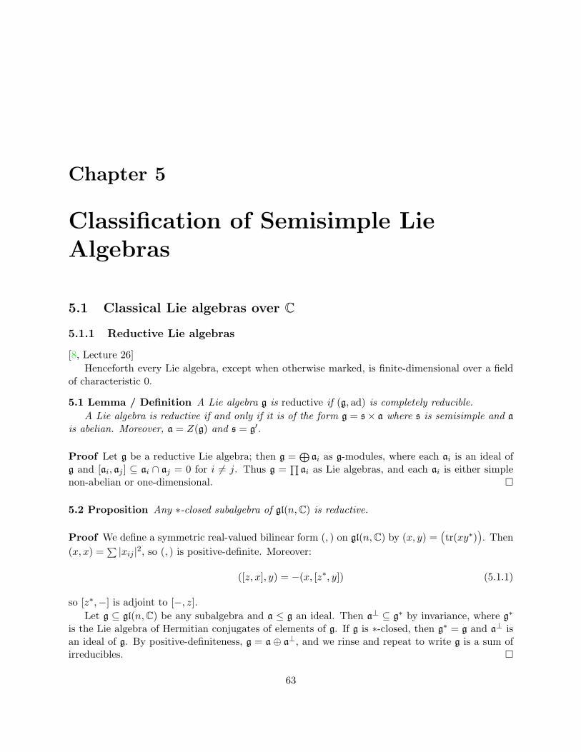
Chapter 5
Classification of Semisimple LieAlgebras
5.1 Classical Lie algebras over C
5.1.1 Reductive Lie algebras
[8, Lecture 26]Henceforth every Lie algebra, except when otherwise marked, is finite-dimensional over a field
of characteristic 0.
5.1 Lemma / Definition A Lie algebra g is reductive if (g, ad) is completely reducible.A Lie algebra is reductive if and only if it is of the form g = s× a where s is semisimple and a
is abelian. Moreover, a = Z(g) and s = g′.
Proof Let g be a reductive Lie algebra; then g =⊕
ai as g-modules, where each ai is an ideal ofg and [ai, aj ] ⊆ ai ∩ aj = 0 for i 6= j. Thus g =
∏ai as Lie algebras, and each ai is either simple
non-abelian or one-dimensional. �
5.2 Proposition Any ∗-closed subalgebra of gl(n,C) is reductive.
Proof We define a symmetric real-valued bilinear form (, ) on gl(n,C) by (x, y) =Ätr(xy∗)
ä. Then
(x, x) =∑ |xij |2, so (, ) is positive-definite. Moreover:
([z, x], y) = −(x, [z∗, y]) (5.1.1)
so [z∗,−] is adjoint to [−, z].Let g ⊆ gl(n,C) be any subalgebra and a ≤ g an ideal. Then a⊥ ⊆ g∗ by invariance, where g∗
is the Lie algebra of Hermitian conjugates of elements of g. If g is ∗-closed, then g∗ = g and a⊥ isan ideal of g. By positive-definiteness, g = a⊕ a⊥, and we rinse and repeat to write g is a sum ofirreducibles. �
63

64 CHAPTER 5. CLASSIFICATION OF SEMISIMPLE LIE ALGEBRAS
5.3 Example The classical Lie algebras sl(n,C) def= {x ∈ gl(n) s.t. trx = 0}, so(n,C) def= {x ∈gl(n) s.t. x+ xT = 0}, and sp(n,C) def= {x ∈ gl(2n) s.t. jx+ xT j = 0} are reductive. Indeed, sincethey have no center except in very low dimensions, they are all semisimple. We will see later thatthey are all simple, except in a few low dimensions.
Since a real Lie algebra g is semisimple if g⊗R C is, the real Lie algebras sl(n,R), so(n,R), andsp(n,R) also are semisimple.
5.1.2 Guiding examples: sl(n) and sp(n) over C
[8, Lectures 27 and 28]Let g = sl(n) or sp(n). We extract an abelian subalgebra h ⊆ g. For sln we use the diagonal
traceless matrices:
hdef=
z1
. . .zn
s.t.∑
zi = 0
(5.1.2)
For sp(n) def= {x ∈ gl(2n) s.t. jx + xT j = 0}, it will be helpful to redefine j. We can use any jwhich defines a non-degenerate antisymmetric bilinear form, and we take:
j =
1
0 . ..
1−1
. .. 0−1
(5.1.3)
Let aR be the matrix a reflected across the antidiagonal. Then we can define sp(n) in block diagonalform:
sp(n) =®ñ
a b
c d
ô∈ M(2n) = M(2,M(n)) s.t. d = −aR, b = bR, c = cR
´(5.1.4)
In this basis, we take as our abelian subalgebra
hdef=
z1
. . . 0zn−zn
0. . .
−z1
(5.1.5)
5.4 Proposition Let g = sl(n) or sp(n). For h ≤ g defined above, the adjoint action ad : h y g
is diagonal.

5.1. CLASSICAL LIE ALGEBRAS OVER C 65
Proof We make explicit the basis of g. For g = sl(n), the natural basis is {eij}i 6=j ∪ {eii −ei+1,i+1}n−1
i=1 , where eij is the matrix with a 1 in the (ij) spot and 0s elsewhere. In particular,{eii − ei+1,i+1}n−1
i=1 is a basis of h. Let h ∈ h be
h =
z1
. . .zn
(5.1.6)
Then [h, eij ] = (zi − zj)eij , and [h, h′] = 0 when h′ ∈ h.For g = sp(n), the natural basis suggested by equation 5.1.4 is®aij
def=ñeij 00 −en+1−j,n+1−i
ô´∪®bij
def=ñ
0 eij + en+1−j,n+1−i0 0
ôs.t. i+ j ≤ n+ 1
´∪®cij
def=ñ
0 0eij + en+1−j,n+1−i 0
ôs.t. i+ j ≤ n+ 1
´(5.1.7)
Of course, when i = j, then®ñ
eii 00 −en+1−i,n+1−i
ô´is a basis of h. Let h ∈ h be given by
h =
z1
. . . 0zn−zn
0. . .
−z1
(5.1.8)
Then [h, aij ] = (zi − zj)aij , [h, bij ] = (zi + zj)bij , and [h, cij ] = (−zi − zj)cij . �
5.5 Definition Let h be a maximal abelian subalgebra of a finite-dimensional Lie algebra g so thatad : h y g is diagonalizable, so diagonal in an eigenbasis. Write h∗ for the vector space dual to h.Each eigenbasis element of g defines an eigenvalue to each h ∈ h, and this assignment is linear inh; thus, the eigenbasis of g picks out a vector α ∈ h∗. The set of such vectors are the roots of thepair (g, h).
We will refine this definition in Definition 5.41, and we will prove that the set of roots of a semisimpleLie algebra g is determined up to isomorphism by g (in particular, it does not depend on thesubalgebra h).
5.6 Example When g = sl(n) and h is as above, the roots are {0} ∪ {zi − zj}i 6=j , where {zi}ni=1
are the natural linear functionals h → C. When g = sp(n) and h is as above, the roots are{0} ∪ {±2zi} ∪ {±zi ± zj}i 6=j .
5.7 Lemma / Definition Let g and h ≤ g as in Definition 5.5. Then the roots break g intoeigenspaces:
g =⊕
α a root
gα = h⊕⊕
α 6=0 a root
gα (5.1.9)

66 CHAPTER 5. CLASSIFICATION OF SEMISIMPLE LIE ALGEBRAS
In particular, since h is a maximal abelian subalgebra, the 0-eigenspace of hy g is precisely g0 = h.Then the spaces gα are the root spaces of the pair (g, h). By the Jacobi identity, [gα, gβ] ⊆ gα+β.
5.8 Lemma When g = sl(n) or sp(n) and h is as above, then for α 6= 0 the root space gα ⊆ g isone-dimensional. Let hα
def= [gα, g−α]. Then hα = h−α is one-dimensional, and gα ⊕ g−α ⊕ hα is asubalgebra of g isomorphic to sl(2).
Proof For each root α, pick a basis element g±α ∈ g±α (in particular, we can use the eigenbasisof h y g given above), and define hα
def= [gα, g−α]. Define α(hα) = a so that [hα, g±α] = ±agα; onecan check directly that a 6= 0. For the isomorphism, we use the fact that C is algebraically closed.�
5.9 Definition Let g and h ≤ g as in Definition 5.5. The rank of g is the dimension of h, orequivalently the dimension of the dual space h∗.
5.10 Example The Lie algebras sl(3) and sp(2) are rank-two. For g = sl(3), the dual space h∗
to h spanned by the vectors z1 − z2 and z2 − z3 naturally embeds in a three-dimensional vectorspace spanned by {z1, z2, z3}, and we choose an inner product on this space in which {zi} is anorthonormal basis. Let α1 = z1− z2, α2 = z2− z3, and α3 = z1− z3. Then the roots {0,±αi} forma perfect hexagon:
• 0
•α2
•α3
•α1
•−α2
•−α3
•−α1
(5.1.10)
For g = sp(2), we have h∗ spanned by {z1, z2}, and we choose an inner product in which this is
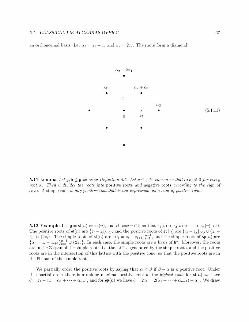
5.1. CLASSICAL LIE ALGEBRAS OVER C 67
an orthonormal basis. Let α1 = z1 − z2 and α2 = 2z2. The roots form a diamond:
•0
·z2
·z1
•α2
•α1
•α2 + α1
•α2 + 2α1
•
••
•
(5.1.11)
5.11 Lemma Let g, h ≤ g be as in Definition 5.5. Let v ∈ h be chosen so that α(v) 6= 0 for everyroot α. Then v divides the roots into positive roots and negative roots according to the sign ofα(v). A simple root is any positive root that is not expressible as a sum of positive roots.
5.12 Example Let g = sl(n) or sp(n), and choose v ∈ h so that z1(v) > z2(v) > · · · > zn(v) > 0.The positive roots of sl(n) are {zi − zj}i<j , and the positive roots of sp(n) are {zi − zj}i<j ∪ {zi +zi} ∪ {2zi}. The simple roots of sl(n) are {αi = zi − zi+1}n−1
i=1 , and the simple roots of sp(n) are{αi = zi − zi+1}n−1
i=1 ∪ {2zn}. In each case, the simple roots are a basis of h∗. Moreover, the rootsare in the Z-span of the simple roots, i.e. the lattice generated by the simple roots, and the positiveroots are in the intersection of this lattice with the positive cone, so that the positive roots are inthe N-span of the simple roots.
We partially order the positive roots by saying that α < β if β − α is a positive root. Underthis partial order there is a unique maximal positive root θ, the highest root; for sl(n) we haveθ = z1 − zn = α1 + · · ·+ αn−1, and for sp(n) we have θ = 2z1 = 2(α1 + · · ·+ αn−1) + αn. We draw

68 CHAPTER 5. CLASSIFICATION OF SEMISIMPLE LIE ALGEBRAS
these partial orders:
•α1
•α2
•α3
· · · •αn−1
• •• • • •• • •• •
· · ·
•θ=α1+···+αn−1
•α1+α2
•αn−2+αn−1
sl(n)
•α1
•α2
· · · •αn−1
•αn
• • • •• • • •• • • •• • •• • •• •• •••
•
•
•
•
· · ·
•θ=2(α1+···+αn−1)+αn
sp(n)
To make this very clear, we draw the rank-three pictures fully labeled (edges by the differencebetween consecutive nodes):
•α1 = z1 − z2
•α2 = z2 − z3
•α3 = z3 − z4
•z1 − z3
•z2 − z4
•θ = z1 − z4
α2 α1 α3 α2
α3 α1
sl(4)

5.1. CLASSICAL LIE ALGEBRAS OVER C 69
•α1 = z1 − z2
•α2 = z2 − z3
•α3 = 2z3
•z1 − z3
• z2 + z3
•z1 + z3
• 2z2
•z1 + z2
• θ = 2z1
α2 α1 α3 α2
α3 α1
α2 α1
α2
α1
sp(3)
Using these pictures of sl(n) and sp(n), we can directly prove the following:
5.13 Proposition The Lie algebras sl(n,C) and sp(n,C) are simple.
Proof Let g = sl(n) or sp(n), and h, the systems of positive and simple roots, and θ the highestroot as above. Recall that for each root α 6= 0, the root space gα is one-dimensional, and we pickan eigenbasis {gα}α 6=0 ∪ {hi}rank
i=1 for the action h y g.Let x ∈ g. It is a standard exercise from linear algebra that hx is the span of the eigenvectros
gα, α 6= 0, for which the coefficient of x in the eigenbasis is non-zero. In particular, if x ∈ g r h,then [h, x] includes some gα. By switching the roles of positive and negative roots if necessary, wecan assure that α is positive; thus [h, x] ⊇ gα for some positive α.
One can check directly that if α, β, α + β are all nonzero roots, then [gα, gβ] = gα+β. Inparticular, for any positive root α, θ − α is a positive root, and so [g, gα] ⊇ [gθ−α, gα] = gθ. Inparticular, gθ ∈ [g, x].
But [gθ−α, gθ] = gα, and so [g, gθ] generates all gα for α a positive root. We saw already(Lemma 5.8) that [gα, g−α] = hα is non-zero, and that [g±α, hα] = g±α. Thus [g, gα] ⊇ g−α, and inparticular gθ generates every gα for α 6= 0, and every hα. Then gθ generates all of g.
Thus x generates all of g for any x ∈ g r h. If x ∈ h, then α(x) 6= 0 for some α, and then[gα, x] = gα, and we repeat the proof with some nonzero element of gα. Hence g is simple. �
When g = sl(n), let εi refer to the matrix eii, and when g = sp(n), let εi refer to the matrixñeii 00 −en+1−i,n+1−i
ô. We construct a linear isomorphism h∗
∼→ h by assigning an element α∨i of
h to each simple root αi as follows: to αi = zi − zi+1 for 1 ≤ i ≤ n − 1 we assign α∨i = εi − εi+1,and to αn = 2zn a root of sp(n) we assign α∨n = εn. In particular, αi(hi) = 2 for each simple root.We define the Cartan matrix a by aij
def= αi(hj).

70 CHAPTER 5. CLASSIFICATION OF SEMISIMPLE LIE ALGEBRAS
5.14 Example For sl(n), we have the following (n− 1)× (n− 1) matrix:
a =
2 −1 0 . . . 0
−1 2 −1...
0 −1. . . . . . 0
.... . . 2 −1
0 . . . 0 −1 2
(5.1.12)
For sp(n), we have the following n× n matrix:
a =
2 −1 0 . . . 0 0
−1 2 −1...
...
0 −1. . . . . . 0
......
. . . 2 −1 00 . . . 0 −1 2 −10 . . . . . . 0 −2 2
(5.1.13)
To each of the above matrices we associate a Dynkin diagram. This is a graph with a nodefor each simple root, and edges assigned by: i and j are not connected if aij = 0; they are
singly connected if aij is a blockñ
2 −1−1 2
ô; we put a double arrow from j to i when the (i, j)-
block isñ
2 −1−2 2
ô. So for sl(n) we get the graph • • · · · • , and for sp(n) we get
• • · · · •• .
5.15 Lemma / Definition The identification h∗∼→ h lets us construct reflections of h∗ by si :
α 7→ α−〈α, α∨i 〉α, where 〈, 〉 is the pairing h∗⊗h→ C that we had earlier written as 〈α, β〉 = α(β).These reflections generated the Weyl group W .
For each of sl(n) and sp(n), let R ⊆ h∗ be the set of roots and W the Weyl group. ThenW y R r {0}. In particular, for sl(n), we have W = Sn the symmetric group on n letters, wherethe reflection (i, i+ 1) acts as si; W y Rr{0} is transitive. For sp(n), we have W = Snn (Z/2)n,the hyperoctahedral group, generated by the reflections si = (i, i+ 1) ∈ Sn and sn the sign change,and the action W y Rr {0} has two orbits.
We will spend the rest of this chapter showing that the picture of sl(n) and sp(n) in this sectionis typical of simple Lie algebras over C.
5.2 Representation Theory of sl(2)
[8, Lectures 28 and 29]Our hero for this section is the Lie algebra sl(2,C) def= 〈e, h, f : [e, f ] = h, [h, e] = 2e, [h, f ] =
−2f〉 = {x ∈ M(2,C) s.t. trx = 0}.

5.2. REPRESENTATION THEORY OF sl(2) 71
5.16 Example As a subalgebra of M(2,C), sl(2) has a tautological representation on C2, given
by E 7→ñ
0 10 0
ô, F 7→
ñ0 01 0
ô, and H 7→
ñ1 00 −1
ô. Let v0 and v1 be the basis vectors of C2.
Then the representation sl(2) y C2 has the following picture:
•v0
•v1
H
H
FE (5.2.1)
This is the infinitesimal verion of the action SL(2) y C2 given by
(exp(−te))ñxy
ô=ñ
1 −t0 1
ô ñxy
ô=ñx− tyy
ô(5.2.2)
d
dt
∣∣∣∣t=0
exp(−te) =®ñ
xy
ô7→ñ−y0
ô´(5.2.3)
d
dt
∣∣∣∣t=0
exp(−tf) =®ñ
xy
ô7→ñ
0−x
ô´(5.2.4)
5.17 Example Since SL(2) y C2, it acts also on the space of functions on C2; by the previouscalculations, we see that the action is:
e = −y∂x, f = −x∂y, h = −x∂x + y∂y (5.2.5)
These operations are homogenous — they preserve the total degree of any polynomial — and sothe symmetric tensor product Sn(C2) = {homogeneous polynomials of degree n in x and y} is asubmodule of SL(2) y {functions}. Let vi
def=(ni
)xiyn−i be a basis vector in Sn(Cx ⊕ Cy). Then
the action SL(2) y S2(C2) has the following picture:
•yn = v0
•nxyn−1 = v1
•(n
2
)x2yn−2 = v2
...
•( nn−1
)xn−1y = vn−1
•xn = vn
h=n
h=n−2
h=n−4
h=2−n
h=−n
f=1
f=2
f=n
n=e
n−1=e
1=e
(5.2.6)
Let us call this module Vn. Then Vn is irreducible, because applying e enough times to any non-zeroelement results in a multiple of v0, and v0 generated the module.

72 CHAPTER 5. CLASSIFICATION OF SEMISIMPLE LIE ALGEBRAS
5.18 Proposition Let V be any (n+ 1)-dimensional irreducible module over sl(2). Then V ∼= Vn.
Proof Suppose that v ∈ V is an eigenvector of h, so that hv = λv. Then hev = [h, e]v + ehv =2ev + λev, so ev is an h-eigenvector with eigenvalue λ + 2. Similarly, fv is an h-eigenvector witheigenvalue λ − 2. So the space spanned by h-eigenvectors of V is a submodule of V ; by theirreducibility of V , and using the fact that h has at least one eigenvector, this submodule must bethe whole of V , and so h acts diagonally.
By finite-dimensionality, there is an eigenvector v0 of h with the highest eigenvalue, and soev0 = 0. By Theorem 3.24, {fkelhm} spans Usl(2), and so {vi
def= f iv0/i!} is a basis of V (byirreducibility, V is generated by v0). In particular, vn = fnv0/n!, the (n+1)st member of the basis,has fvn = 0, since V is (n+ 1)-dimensional.
We compute the action of e by induction, using the fact that hvk = (λ0 − 2k)vk:
ev0 = 0 (5.2.7)ev1 = efv0 = [e, f ]v0 + fev0 = hv0 = λ0v0 (5.2.8)ev2 = efv1/2 = [e, f ]v1/2 + fev1/2 = hv1/2 + fλ0v0/2
= (λ0 − 2)v1/2 + λ0v1/2 = (λ0 − 1)v1 (5.2.9). . .
evk = efvk−1/k = hvk−1/k + fevk−1/k = (λ0 − 2k + 2)vk−1/k + (λ0 − k + 2)fvk−2/k
=Ä(λ0 − 2k + 2)/k + (k − 1)(λ0 − k + 2)/k
ävk−1 = (λ0 − k + 1)vk−1 (5.2.10)
But fvn = 0, and so:
0 = efvn = [e, f ]vn + fevn = hvn + (λ0 − n+ 1)fvn−1
= (λ0 − 2n)vn + (λ0 − n+ 1)nvn =Ä(n+ 1)λ0 − (n+ 1)n
ävn (5.2.11)
Thus λ0 = n and V is isomorphic to Vn defined in equation 5.2.6. �
5.3 Cartan subalgebras
5.3.1 Definition and Existence
[8, Lectures 29 and 30]
5.19 Lemma Let h be a nilpotent Lie algebra over a field K, and h y V a finite-dimensionalrepresentation. For h ∈ h and λ ∈ C, define Vλ,h = {v ∈ V s.t. ∃n s.t. (h− λ)nv = 0}. Then Vλ,his an h-submodule of V .
Proof Let ad : h y h be the adjoint action; since h is nilpotent, adh ∈ End(h) is a nilpotentendomorphism. Define h(m)
def= kerÄ(adh)m
ä; then h(m) = h for m large enough. We will show that
h(m)Vλ,h ⊆ Vλ,h by induction on m; when m = 0, h(0) = 0 and the statement is trivial.

5.3. CARTAN SUBALGEBRAS 73
Let y ∈ h(m), whence [h, y] ∈ h(m−1), and let v ∈ Vλ,h. Then (h− λ)nv = 0 for n large enough,and so
(h− λ)nyv = y(h− λ)nv + [(h− λ)n, y]v (5.3.1)= 0 + [(h− λ)n, y]v (5.3.2)
=∑
k+1=n−1
(h− λ)k[h, y](h− λ)lv (5.3.3)
since [λ, y] = 0. By increasing n, we can assure that for each term in the sum at least one of thefollowing happens: l is large enough that (h− λ)lv = 0, or k is large enough that (h− λ)kVλ,h = 0.The large-l terms vanish immediately; the large-k terms vanish upon realizing that (h−λ)Vh,λ ⊆ Vh,λby definition and [h, y]Vh,λ ⊆ h(m−1)Vh,λ ⊆ Vh,λ by induction on m. �
5.20 Corollary Let h be a nilpotent Lie algebra over K, h y V a finite-dimensionalrepresentation,and λ : h→ K a linear map. Then Vλ
def=⋂h∈h Vλ(h),h is an h-submodule of V .
5.21 Proposition Let h be a finite-dimensional nilpotent Lie algebra over an algebraically closedfield K of characteristic 0, and V a finite-dimensional h-module. For each λ ∈ h∗, define Vλ as inCorollary 5.20. Then V =
⊕λ∈h∗ Vλ.
Proof Let h1, . . . , hk ∈ h, and let Hk ⊆ h be the linear span of the hi. Let W def=⋂ki=1 Vλ(hi),hi .
It follows from Theorem 4.37 that W =⋂h∈H Vλ(h),h, since we can choose a basis of V in which
h y V by upper-triangular matrices.We have seen already that W is a submodule of V . Let hk+1 6∈ Hk; then we can decompose W
into generalized eigenspaces of hk+1. We proceed by induction on k until we have a basis of h. �
5.22 Definition For λ ∈ h∗, the space Vλ in Corollary 5.20 is a weight space of V , and V =⊕λ∈h∗ Vλ the weight space decomposition.
5.23 Lemma Let h be a finite-dimensional nilpotent Lie algebra over an algebraically closed fieldof characteristic 0, and let V and W be two finite-dimensional h modules. Then the weight spacesof V ⊗W are given by (V ⊗W )λ =
⊕α+β=λ Vα ⊗Wβ.
Proof h(v ⊗ w) = hv ⊗ w + v ⊗ hw �
5.24 Corollary Let g be a finite-dimensional Lie algebra over an algebraically closed field of char-acteristic 0, and h ⊆ g a nilpotent subalgebra. Then the weight spaces of ad : h y g satisfy[gα, gβ] ⊆ gα+β.
5.25 Proposition Let g be a finite-dimensional Lie algebra over an algebraically closed field ofcharacteristic 0, and let h ⊆ g be a nilpotent subalgebra. The following are equivalent:
1. h = N(h) def= {x ∈ g s.t. [x, h] ⊆ h}, the normalizer of h in g.
2. h = g0 is the 0-weight space of ad : hy g.

74 CHAPTER 5. CLASSIFICATION OF SEMISIMPLE LIE ALGEBRAS
Proof Define N (i) def= {x ∈ g s.t. (ad h)ix ⊆ h}. Then N (0) = h and N (1) = N(h), and N (i) ⊆N (i+1). By finite-dimensionality, the sequence N (0) ⊆ N (1) ⊆ . . . must eventually stabilize. Bydefinition
⋃N (i) = g0, so 2. implies 1. But N (i+1) = N(N (i)), and so 1. implies 2. �
5.26 Definition A subalgebra h of g satisfying the equivalent conditions of Proposition 5.25 is aCartan subalgebra of g.
5.27 Theorem (Existence of a Cartan Subalgebra) Every finite-dimensional Lie algebra overan algebraically closed field of characteristic 0 has a Cartan subalgebra.
Before we prove this theorem, we will need some definitions and lemmas.
5.28 Definition Let K be a field; we say that X ⊆ Kn is Zariski closed if X = {x ∈ Kn s.t. pi(x) =0 ∀i} for some possibly infinite set {pi} of polynomials in K[x1, . . . , xn]. A subset X ⊆ Kn is Zariskiopen if Kn rX is Zariski closed.
5.29 Lemma If K is infinite and U, V ⊆ Kn are two non-empty Zariski open subsets, then U ∩ Vis non-empty.
Proof Let U def= Kn r U and similarly for V . Let u ∈ U and v ∈ V . If u = v we’re done,and otherwise consider the line L ⊆ Kn passing through u and v, parameterized K ∼→ L byt 7→ tu + (1 − t)v. Then L ∩ U and L ∩ V are finite, as their preimages under K → L are loci ofpolynomials. Since K is infinite, L contains infinitely many points in U ∩ V . �
5.30 Lemma / Definition Let g be a finite-dimensional Lie algebra over an algebraically closedfield of characteristic 0. An element x ∈ g is regular if g0,x has minimal dimension. If x is regular,then g0,x is a nilpotent subalgebra of g.
Proof We will write h for g0,x. That h is a subalgebra follows from Corollary 5.24. Suppose
that h is not nilpotent, and let U def= {h ∈ h s.t. adh|h if not nilpotent} 6= 0. Then U = {h ∈h s.t. (adh|h)d 6= 0} is a Zariski-open subset of h. Moreover, V def= {h ∈ h s.t. h acts invertibly on g/h}is also a non-empty Zariski-open subset of h, where V is the quotient of h-modules; it is non-emptybecause x ∈ V . By Lemma 5.29 (recall that any algebraically closed field is infinite), there existsy ∈ U ∩ V . Then ad y preserves gα,x for every α, as y ∈ h = g0,x, and y acts invertibly on everygα,x for α 6= 0. Theng0,y ⊆ g0,x = h, but y ∈ U and so g0,y 6= h. This contradicts the minimality ofh. �
Proof (of Theorem 5.27) We let g, x ∈ g, and h = g0,x be as in Lemma/Definition 5.30. Thenh ⊆ g0,h because h is nilpotent, and g0,h ⊆ g0,x = h because x ∈ h. Thus h is a Cartan subalgebraof g. �
We mention one more fact about the Zariski topology:
5.31 Lemma Let U by a Zariski open set over C. Then U is path connected.

5.3. CARTAN SUBALGEBRAS 75
Proof Let u, v ∈ U and construct the line L as in the proof of Lemma 5.29. Then L ∩ U isisomorphic to Cr {finite}, and therefore is path connected. �
5.32 Proposition Let g be a finite-dimensional Lie algebra over C. Then all Cartan subalgebrasof g are conjugate by automophisms of g.
Proof Consider ad : g → gl(g). Then ad g ⊆ gl(g) is a Lie subalgebra, and so corresponds toa connected Lie subgroup Int g ⊆ GL(g) generated by exp(ad g). Since g y g be derivations,exp(ad g) y g by automorphisms, and so Int g ⊆ Aut g.
Let h ⊆ g be a Cartan subalgebra, and g =⊕
gα,h the corresponding weight-space decomposi-tion. Since g is finite-dimensional, the set
Rhdef= {h ∈ h s.t. α(h) 6= 0 if α 6= 0 and gα,h 6= 0} = {h ∈ h s.t. g0,h = h} (5.3.4)
is non-empty and open, since we can take α to range over a finite set (by finite-dimensionality).Let σ : Int g× g→ g be the canonical action, and consider the restriction to σ : Int g×Rh → g.
Pick y ∈ Rh and let e ∈ Int g be the identity element. We compute the image of the infinitesimalaction dσ
ÄT(e,y)(Int g×Rh)
ä⊆ Tyg ∼= g. By construction, varying the first component yields an
action by conjugation: x 7→ [x, y]. Thus the image of Te Int g × {0 ∈ TyRh} is (ad y)(g). Since yacts invertibly, (ad y)(g) ⊇ ⊕α 6=0 gα,h. By varying the second coordinate (recall that Rh is open),we see that dσ
ÄT(e,y)(Int g×Rh)
ä⊇ h = g0,h also. Thus dσ
ÄT(e,y)(Int g×Rh)
ä= g = Tyg, and so
the image (Int g)(Rh) contains a neighborhood of y and therefore is open.For each y ∈ g, consider the generalized nullspace g0,y; the dimension of g0,y depends on
the characteristic polynomial of y, and the coefficients of the characteristic polynomial dependpolynomially on the matrix entries of ad y. In particular, dim g0,y ≥ r if and only if the last rcoefficients of the characteristic polynomial of ad y are 0, and so {y ∈ g s.t. dim g0,y ≥ r} is Zariskiclosed. Therefore y 7→ dim g0,y is upper semi-continuous in the Zariski topology. In particular,let r be the minimum value of dim g0,y, which exists since dim g0,y takes values in integers. Then
Reg def= {y ∈ g s.t. dim g0,y = r}, the set of regular elements, is Zariski open and therefore dense.In particular, Reg intersects (Int g)(Rh).
But if y ∈ (Int g)(Rh) then dim g0,y = dim h. Therefore dim h is the minimal value of dim g0,y
and in particular Rh ⊆ Reg. Conversely, Reg =⋃
h′ a CartanRh′ =⋃
h′ a Cartan(Int g)Rh′ .However, Int g is a connected group, Rh is connected being Cn minus some hyperplanes, and
Reg is connected on account of being Zariski open. But the orbits of (Int g)Rh are disjoint, andtheir union is all of Reg, so Reg must consist of a single orbit.
To review: h is Cartan and so contains regular elements of g, and any other regular element of g
is in the image under Int g of a regular element of h. Thus every Cartan subalgebra is in (Int g)h.�
5.3.2 More on the Jordan Decomposition and Schur’s Lemma
[8, Lectures 30 and 31]Recall Theorem 4.50 that every x ∈ End(V ), where V is a finite-dimensional vector spce over
an algebraically closed field, has a unique decomposition x = xs + xn where xs is diagonalizableand xn is nilpotent. We will strengthen this result in the case when x ∈ g → End(V ) and g issemisimple.

76 CHAPTER 5. CLASSIFICATION OF SEMISIMPLE LIE ALGEBRAS
5.33 Lemma Let g be a finite-dimensional Lie algebra over an algebraically closed field, andDer g ⊆ End g the algebra of derivations of g. If x ∈ Der g, then xs, xn ∈ Der g.
Proof For x ∈ Der g, construct the weight-space decomposition g =⊕
λ gλ,x of generalizedeigenspaces of x. Since x is a derivation, the weight spaces add: [gµ,x, gν,x] ⊆ gµ+ν,x. Let y ∈ End g
act as λ on gλ,x; then y is a derivation by the additive property. But y is diagonalizable andcommutes with x, and x− y is nilpotent because all its eigenvalues are 0 so y = xs. �
We have an immediate corollary:
5.34 Lemma / Definition If g is a semisimple finite-dimensional Lie algebra over an algebraicallyclosed field K, then every x ∈ g has a unique Jordan decomposition x = xs + xn such that[xs, xn] = 0, adxs is diagonalizable, and adxn is nilpotent.
Proof If g is semisimple then ad : g → Der g is injective as Z(g) = 0 and surjective becauseDer g/ ad g = Ext1(g,K) = 0. �
5.35 Theorem (Schur’s Lemma over an algebraically closed field) Let U be an algebra overK and algebraically closed field, and let V be an irreducible U -module. Then EndU (V ) = K.
Proof Let φ ∈ EndU (V ) and λ ∈ K an eigenvalue of φ. Then φ − λ is singular and hence 0 byTheorem 4.74. �
5.36 Proposition Let g be a finite-dimensional semisimple Lie algebra over an algebraically closedfield of characteristic 0, and let σ : g y V be a finite-dimensional g module. For x ∈ g, write xs andxn as in Lemma/Definition 5.34, and write σ(x)s and σ(x)n for the diagonalizable and nilpotentparts of σ(x) ∈ gl(g) as given by Theorem 4.50. Then σ(x)s = σ(xs) and σ(x)n = σ(xn).
Proof We reduce to the case when V is an irreducible g-module using Theorem 4.78, and we writeg =
∏gi a product of simples using Corollary 4.61. Then gi y V as 0 for every i except one, for
which the action gi y V is faithful. We replace g by that gi, whence σ : g ↪→ gl(V ) with g simple.It suffices to show that σ(x)s ∈ σ(g), since then σ(xs) = σ(s) for some s ∈ g, σ(x)n =
σ(x) − σ(s) = σ(x − s), and s and n = x − s commute, sum to x, and act diagonalizably andnilpotently since the adjoint action ad : g y g is a submodule of g y gl(V ), so s = xs and n = xn.
By semisimplicity, g = g′ ⊆ sl(V ). By Theorem 5.35, the centralizer of g in gl(V ) consistsof scalars. In characteristic 0, the only scalar in sl(V is 0, so the centralizer of g in sl(V ) is 0.Define the normalizer N(g) = {x ∈ sl(V ) s.t. [x, g] ⊆ g}; then N(g) is a Lie subalgebra of sl(V )containing g, and N(g) acts faithfully on g since the centralizer of g in sl(V ) is 0, and this actionis by derivations. But all derivations are inner, as in the proof of Lemma/Definition 5.34, and soN(g) y g factors through g y g, and hence N(g) = g.
So it suffices to show that σ(x)s ∈ N(g) for x ∈ g. Since σ(x)n is nilpotent, it’s traceless, andhence in sl(V ); then σ(x)s ∈ sl(V ) as well. We construct a generalized eigenspace decomposition ofV with respect to σ(x) : V =
⊕Vλ,x. Then σ(x)s acts on Vλ,x by the scalar λ. We also construct
a generalized eigenspace decomposition g =⊕
gα,x with respect to the adjoint action ad : g y g.Since g ⊆ gl(V ), we have gα,x = g∩EndK(V )α =
⊕HomK(Vλ,x, Vλ+α,x), by tracking the eigenvalues
of the right and left actions of g on V .

5.3. CARTAN SUBALGEBRAS 77
Moreover, ad(σ(x)s) = ad(σ(xs)) because both act by α on HomK(Vλ,x, Vλ+α,x) and hence ongα. Thus σ(x)s fixes g since σ(xs) does. Therefore σ(x)s ∈ N(g). �
5.3.3 Precise description of Cartan subalgebras
[8, Lecture 31]
5.37 Lemma Let g be a semisimple Lie algebra over characteristic 0, h ⊆ g a nilpotent subalgebra,and g =
⊕gα the root space decomposition with respect to h. Then the Killing form β pairs gα
with g−α nondegenerately, and β(gα, gα′) = 0 if α+ α′ 6= 0.
Proof Let x ∈ gα and y ∈ gα′ . For any h ∈ h, (adh− α(h))nx = 0 for some n. So
0 = βÄ(adh− α(h))n x, y
ä= βÄx, (− adh− α(h))n y
ä(5.3.5)
but (− adh− α(h))n is invertible on gα′ unless α′ = −α. Nondegeneracy follows from nondegener-acy of β on all of g. �
5.38 Corollary If g is a finite-dimensional semisimple Lie algebra over characteristic 0, and leth ⊆ g a nilpotent subalgebra, then the largest nilpotency ideal in g0 of the action ad : g0 y g is the0 ideal.
Proof The Killing form β pairs g0 with itself nondegenerately. As β is the trace form of ad : g0 y g,and ad(g)-nilpotent ideal of g0 must be in kerβ = 0. �
5.39 Proposition Let g be a finite-dimensional semisimple Lie algebra over an algebraically closedfield K of characteristic 0, and let h ⊆ g be a Cartan subalgebra. Then h is abelian and ad : h y g
is diagonalizable.
Proof By definition, h is nilpotent and hence solvable, and by Theorem 4.37 we can find a basisof g in which h y g by upper triangular matrices. Thus h′ = [h, h] acts by strictly upper triangularmatrices and hence nilpotently on g. But h = g0, and so h′ = 0 by Corollary 5.38. This proves thath is abelian.
Let x ∈ h. Then adxs = (adx)s acts as α(x) on gα, and in particular xs centralizes h. Soxs ∈ g0 = h and so xn = x − xs ∈ h. But if n ∈ h acts nilpotently on g, then Kn is an idealof h, since h is abelian, and acts nilpotently on g, so Kn = 0 by Corollary 5.38. Thus xn = 0and x = xs. In particular, x acts diagonalizably on g. To show that h acts diagonalizably, we usefinite-dimensionality and the classical fact that if n diagonalizable matrices commute, then theycan by simultaneously diagonalized. �
5.40 Corollary Let g be a finite-dimensional semisimple Lie algebra over an algebraically closedfield of characteristic 0. Then a subalgebra h ⊆ g is Cartan if and only if h is a maximal diagonal-izable abelian subalgebra.

78 CHAPTER 5. CLASSIFICATION OF SEMISIMPLE LIE ALGEBRAS
Proof We first show the maximality of a Cartan subalgebra. Let h be a Cartan subalgebra andh1 ⊇ h abelian. Then h1 ⊆ g0 = h because it normalizes h.
Conversely, let h be a maximal diagonalizable abelian subalgebra of g, and write g =⊕
gα theweight space decomposition of h y g. We want to show that h = g0, the centralizer of h. Pickx ∈ g0; then xs, xn ∈ g0, and so xs ∈ h by maximality. In particular, g0 is spanned by h andad-nilpotent elements. Thus g0 is nilpotent by Theorem 4.25 and therefore solvable, so g′0 actsnilpotently on g. But g′0 is an ideal of g0 that acts nilpotently, so g′0 = 0, so g0 is abelian. Thenany one-dimensional subspace of g0 is an ideal of g0, and a subspace spanned by a nilpotent actsnilpotently, so g0 doesn’t have any nilpotents. Therefore g0 = h. �
5.4 Root systems
5.4.1 Motivation and a Quick Computation
[8, Lectures 31 and 32]In any semisimple Lie algebra over C we can choose a Cartan subalgebra, to which we assign
combinatorial data. Since all Cartan subalgebras are conjugate, this data, called a root system, willnot depend on our choice. Conversely, this data will uniquely describe the Lie algebra, based onthe representation theory of sl(2).
5.41 Definition Let g be a semisimple Lie algebra over C, and h a Cartan subalgebra. The rootspace decomposition of g is the weight decomposition g =
⊕α gα of ad : h y g; each gα is a root
space, and the set of weights α ∈ h∗ that appear in the root space decomposition comprise the rootsof g. By Proposition 5.32 the structure of the set of roots depends up to isomorphism only on g.
5.42 Lemma / Definition Let g be a semisimple Lie algebra over C with Killing form β, h aCartan subalgebra, and xα ∈ gα for α 6= 0. To xα we can associate yα ∈ g−α with β(xα, yα) = −1and to the root α we associate a coroot hα with β(hα,−) = α. Then {xα, yα, hα} span a subalgebrasl(2)α of g isomorphic to sl(2).
Proof That hα and yα are well-defined follows from the nondegeneracy of β. For any h ∈ h, x ∈ gα,and y ∈ g−α, we have
β(h, [x, y]) = β([x, h], y) (5.4.1)= −α(h)β(x, y) (5.4.2)
Thus [x, y] = −β(x, y)hα. Moreover, since xα ∈ gα, [hα, xα] = α(hα)xα, and since yα ∈ g−α,[hα, yα] = −α(hα)yα.
Thus xα, yα, hα span a three-dimensional Lie subalgebra of g, which is isomorphic to eithersl(2) or or the Heisenberg algebra. But in every finite-dimensional representation the Heisenbergalgebra acts nilpotently, whereas ad(hα) ∈ End(g) is diagonalizable. Therefore this subalgebra isisomorphic to sl(2), and α(hα) 6= 0. �
5.43 Corollary Let α be a root of g. Then ±α are the only non-zero roots of g in Cα, anddim gα = 1. In particular, sl(2)α = gα ⊕ g−α ⊕ Chα.

5.4. ROOT SYSTEMS 79
Proof We consider jαdef=⊕
α′∈Cαr{0} gα′ ⊕ Chα; it is a subalgebra of g and an sl(2)α-submodule,since [gα, gα′ ] ⊆ gα+α′ , and hcα = chα for c ∈ C. Let α′ ∈ Cα r {0} be a root; as a weight of thesl(2)α representation, we see that α′ ∈ Zα/2. If any half-integer multiple of α actually appears,then α/2 appears, and by switching α to α/2 if necessary we can assure that jα contains onlyrepresentations V2m. But each V2m has contributes a basis vector in weight 0, and the only partof jα in weight 0 is Chα. Therefore jα is irreducible as an sl(2)α module, contains sl(2)α, and soequals sl(2)α. �
5.44 Corollary The roots α span h∗, and the coroots hα span h.
Proof We let α range over the non-zero roots. Then⋂α 6=0
kerα = Z(g) = 0 (5.4.3)
∑α 6=0
Chα = g′ ∩ h = h (5.4.4)
That β−1 : α 7→ hα is a linear isomorphism h∗ → h completes the proof. �
5.45 Proposition Let g be a finite-dimensional semisimple Lie algebra over C, and h ⊆ g a Cartansubalgebra. Let R ⊆ h∗ be the set of nonzero roots and R∨ ⊆ h the set of nonzero coroots. Thenα 7→ α∨
def= 2hαα(hα) defines a bijection ∨ : R→ R∨, and the triple (R,R∨,∨) comprise a root system
in h.
We will define the words “root system” in the next section to generalize the data already computed.
5.4.2 The Definition
[8, Lecture 33]
5.46 Definition A root system is a complex vector space h, a finite subset R ⊆ h∗, a subsetR∨ ⊆ h, a bijection ∨ : R→ R∨, subject to
RS1 〈α, β∨〉 ∈ Z
RS2 R = −R and R∨ = −R∨, with (−α)∨ = −(α∨)
RS3 〈α, α∨〉 = 2
RS4 If α, β ∈ R are not proportional, then (β + Cα) ∩R consists of a “string”:¨(β + Cα) ∩R,α∨
∂= {m,m− 2, . . . ,−m+ 2,−m} (5.4.5)
Nondeg R spans h∗ and R∨ spans h
Reduced Cα ∩R = {±α} for α ∈ R.
80 CHAPTER 5. CLASSIFICATION OF SEMISIMPLE LIE ALGEBRAS
Two root systems are isomorphic if there is a linear isomorphism of the underlying vector spaces,inducing an isomorphism on dual spaces, that carries each root system to the other. The rank of aroot system is the dimension of h.
5.47 Definition Given a root system (R,R∨) on a vector space h, the Weyl group W ⊆ GL(h∗)is the group generated by the reflections sα : λ 7→ λ− 〈λ, α∨〉α as α ranges over R.
5.48 Proposition 1. It follows from RS3 that s2α = e ∈W for each root α.
2. It follows from RS4 that WR = R. Thus W is finite. Moreover, W preserves h∗R, the R-spanof R.
3. The W -average of any positive-definite inner product on h∗R is a W -invariant positive-definiteinner product. Let (, ) be a W -invariant positive-definite inner product. Then sα is orthogonalwith respect to (, ), and so sα : λ 7→ λ− 2(λ,α)
(α,α) α. This inner product establishes an isomorphism
h∼→ h∗, under which α∨ 7→ 2α/(α, α).
4. Therefore Reduced holds with R replaced by R∨ if it holds at all.
5. Let W act on h dual to its action on h∗. Then w(α∨) = (wα)∨ for w ∈W and α ∈ R. Thusswα = wsαw
−1.
6. If V ⊆ h∗ is spanned by any subset of R, then R ∩ V and its image under ∨ form anothernondegenerate root system.
7. Two root systems with the same Weyl group and lattices are related by an isomorphism.
5.49 Definition Let R be a root system in h∗. Define the weight lattice to be Pdef= {λ ∈
h∗ s.t. 〈λ, α∨〉 ∈ Z∀α∨ ∈ R∨} and the root lattice Q to be the Z-span of R. Then RS1 im-plies that R ⊆ Q ⊆ P ⊆ h∗; by Nondeg, both P and Q are of full rank and so the index P : Q isfinite. We define the coweight lattice to be P∨ and the coroot lattice to be Q∨.
5.4.3 Classification of rank-two root systems
By Reduced, there is a unique rank-one root system up to isomorphism, the root system of sl(2).Let R be a rank-two root system; then its Weyl group W is a finite subgroup W ⊆ GL(2,R)
generated by reflections. The only finite subgroups of GL(2,R) are the cyclic and dihedral groups;only the dihedral groups are generated by reflections, and so W ∼= D2m for some m. Moreover, Wpreserves the root lattice Q.
5.50 Lemma The only dihedral groups that preserve a lattice are D4, D6, D8, and D12.
Proof Let rθ be a rotation by θ. Its eigenvalues are e±iθ, and so tr(rθ) = 2 cos θ. If rθ preservesa lattice, its trace must be an integer, and so 2 cos θ ∈ {1, 0,−1,−2}, as 2 cos θ = 2 correspondsto the identity rotation, and | cos θ| ≤ 1. Therefore θ ∈ {π, 2π/3, π/2, π/3}, i.e. θ = 2π/m form ∈ {2, 3, 4, 6}, and the only valid dihedral groups are D2m for these values of m. �

5.4. ROOT SYSTEMS 81
5.51 Corollary There are four rank-two root systems, corresponding to the rectangular lattice, thesquare lattice, and the hexagonal lattice twice:
θ = π θ = 2π/3 θ = π/2 θ = π/3
For each dihedral group, we can pick two reflections α1, α2 with a maximally obtuse angle;these generate W and the lattice. On the next page we list the four rank-two root systems withcomments on their corresponding Lie groups:

82 CHAPTER 5. CLASSIFICATION OF SEMISIMPLE LIE ALGEBRAS
m Picture Name notes
2α2
α1A1 ×A1 = D2 corresponding to the Lie algbera sl(2)× sl(2) = so(4)
3α2
α1A2 corresponding to sl(3) acting on the traceless diagonals
4α2
α1B2 = C2
so(5) = sp(4). (When we get higher up, the Bs and Cs willseparate, and we will have a new sequence of Ds.)
6α2
α1G2
a new simple algebra of dimension 14 = number of roots plusdimension of root space. We will see later that its smallestrepresentation has dimension 7. There are many descriptionsof this representation and the corresponding Lie algebra; theseven-dimensional representation comes from the Octonians,a non-associative, non-commutative “field”, and G2 is theautomorphism group of the pure-imaginary part of the Oc-tonians.

5.4. ROOT SYSTEMS 83
5.52 Lemma / Definition The axioms of a finite root system are symmetric under the inter-change R↔ R∨. This interchange assigns a dual to each root system.
Proof Only RS4 is not obviously symmetric. We did not use RS4 to classify the two-dimensionalroot systems; we needed only a corollary:
RS4’ W (R) = R,
which is obviously symmetric. But RS4 describes only the two-dimensional subspaces of a rootsystem, and every rank-two root system with RS4’ replacing RS4 in fact satisfies RS4. Thissuffices to show that RS4’ implies RS4 for finite root systems. �
We remark that the statement is false for infinite root systems, and we presented the definitionwe did to accommodate the infinite case. We will not discuss infinite root systems further.
5.4.4 Positive roots
[8, Lecture 34]1
5.53 Definition A positive root system consists of a (finite) root system R ⊆ h∗R and a vectorv ∈ hR so that α(v) 6= 0 for every root α ∈ R. A root α ∈ R is positive if α(v) > 0, and negativeotherwise. Let R+ be the set of positive roots and R− the set of negative ones; then R = R+ tR−,and by RS2, R+ = −R−.
The R≥0-span of R+ is a cone in h∗R, and we let ∆ be the set of extremal rays in this cone.Since the root system is finite, extremal rays are generated by roots, and we use Reduced to identifyextremal rays with positive roots. Then ∆ ⊆ R is the set of simple roots.
5.54 Lemma If α and β are two simple roots, then α− β is not a root. Moreover, (α, β) ≤ 0 forα 6= β.
Proof If α − β is a positive root, then α = β + (α − β) is not simple; if α − β is negative then βis not simple.
For the second statement, assume that α and β are any two roots with (α, β) > 0. If α 6= β,then they cannot be proportional, and we assume without loss of generality that (α, α) ≤ (β, β).Then sβ(α) = α − 2(α,β)
(β,β) β = α − β, because 2(α, β)/(β, β) = 〈α, β∨〉 is a positive integer strictlyless than 2. Thus α− β is a root if (α, β) > 0. �
5.55 Lemma Let Rn have a positive definite inner product (, ), and suppose that v1, . . . , vn ∈ Rnsatisfy (vi, vj) ≤ 0 if i 6= j, and such that there exists v0 with (v0, vi) > 0 for every i. Then{v1, . . . , vn} is an independent set.
Proof Suppose that 0 = c1v1+· · ·+cnvn. Renumbering as necessary, we assume that c1, . . . , ck ≥ 0,and ck+1, . . . , cn ≤ 0. Let v = c1v1 + · · · + ckvk = |ck+1|vk+1 + · · · + |cn|vn. Then 0 ≤ (v, v) =
1I missed a few proofs from class. In particular, the proofs of Lemma 5.54 and Lemma 5.55 are reproduced from[11, page 156].

84 CHAPTER 5. CLASSIFICATION OF SEMISIMPLE LIE ALGEBRAS
(∑ki=1 civi,
∑nj=k+1−ckvk) =
∑j,k |cicj |(vi, vj) ≤ 0, which can happen only if v = 0. But then
0 = (v, v0) =∑ki=1 ci(vi, v0) > 0 unless all ci are 0 for i ≤ k. Similarly we must have cj = 0 for
j ≥ k + 1, and so {vi} is independent. �
5.56 Corollary In any positive root system, the set ∆ of simple roots is a basis of h∗.
Proof By Lemma 5.54, ∆ satisfies the conditions of Lemma 5.55 and so is independent. But ∆generates R+ and hence R, and therefore spans h∗. �
5.57 Lemma Let ∆ = {α1, . . . , αn} be a set of vectors in Rm with inner product (, ), and assumethat αi are all on one side of a hyperplane: there exists v such that (αi, v) > 0 ∀i. Let W be the groupgenerated by reflections Sαi. Let R+ be any subset of R≥0∆ r {0} such that si(R+ r {αi}) ⊆ R+
for each i, and such that the set of heights {(α, v)}α∈R+ ⊆ R≥0 is well-ordered. Then R+ ⊆W (∆).
Proof Let β ∈ R+. We proceed by induction on its height.There exists i such that (αi, β) > 0, because if (β, αi) ≤ 0 ∀i, then (β, β) = 0 since β is a
positive combination of the αis. Thus si(β) = β − (positive)αi; in particular,Äv, si(β)
ä< (v, β).
If β 6= αi, then si(β) ∈ R+ by hypothesis, so by induction si(β) ∈ W (∆), and hence β =si(si(β)) ∈W (∆). If β = αi, it’s already in W (∆). �
5.58 Corollary Let R be a finite root system, R+ a choice of positive roots, and ∆ the correspond-ing set of simple roots. Then R = W (∆), and the set {sαi}αi∈∆ generates W .
5.59 Corollary Let R be a finite root system, R+ a choice of positive roots, and ∆ the correspond-ing set of simple roots. Then R ⊆ Z∆ and R+ ⊆ Z≥0∆.
5.60 Proposition Let R be a finite root system, and R+ and R′+ two choices of positive roots.Then R+ and R′+ are W -conjugate.
Proof Let ∆ be the set of simple roots corresponding to R+. If ∆ ⊆ R′+, then R+ ⊆ R′+. ThenR− ⊆ R′− by negating, and R+ ⊇ R′+ by taking complements, so R+ = R′+.
Suppose αi ∈ ∆ but αi 6∈ R′+, and consider the new system of positive roots si(R′+), wheresi = sαi is the reflection corresponding to αi. Then si(R′+)∩R+ ⊇ si(R′+ ∩R+), because a systemof roots that does not contain αi does not lose anything under si. But αi ∈ R′−, so −αi ∈ R′+, andso αi ∈ si(R′+) and hence in si(R′+) ∩R+. Therefore
∣∣∣si(R′+) ∩R+
∣∣∣ > ∣∣∣R′+ ∩R+
∣∣∣.If si(R′+) 6= R+, then we can find αj ∈ ∆ r si(R′+). We repeat the argument, at each step
making the set∣∣∣w(R′+) ∩ R+
∣∣∣ strictly bigger, where w = · · · sjsi ∈ W . Since R+ is a finite set,eventually we cannot get any bigger; this can only happen when ∆ ⊆ w(R′+), and so R+ = w(R′+).�
5.5 Cartan Matrices and Dynkin Diagrams
5.5.1 Definitions
[8, Lecture 34]

5.5. CARTAN MATRICES AND DYNKIN DIAGRAMS 85
5.61 Definition A finite-type Cartan matrix of rank n is an n × n matrix aij satisfying the fol-lowing:
• aii = 2 and aij ∈ Z≤0 for i 6= j.
• a is symmetrizable: there exists an invertible diagonal matrix d with da symmetric.
• a is positive: all principle minors of a are positive.
An isomorphism between Cartan matrices aij and bij is a permutation σ ∈ Sn such that aij = bσi,σj.
5.62 Lemma / Definition Let R be a finite root system, R+ a system of positive roots, and∆ = {α1, . . . , αn} the corresponding simple roots. The Cartan matrix of R is the matrix aij
def=〈αj , α∨i 〉 = 2(αi, αj)/(αi, αi).
The Cartan matrix of a root system is a Cartan matrix. It depends (up to isomorphism) only onthe root system. Conversely, a root system is determined up to isomorphism by its Cartan matrix.
Proof That the Cartan matrix depends only on the root system follows from Proposition 5.60.That the Cartan matrix determines the root system follows from Corollary 5.58.
Given a choice of root system and simple roots, let didef= (αi, αi)/2, and let dij
def= diδij be thediagonal matrix with the dis on the diagonal. Then d is invertible because di > 0, and da = (αi, αj)is obviously symmetric. Let I ⊆ {1, . . . , n}; then the I × I principle minor of da is just
∏i∈I di
times the corresponding principle minor of a. Since di > 0 for each i and da is the matrix of apositive-definite symmetric bilinear form, we see that a is positive. �
5.5.2 Classification of finite-type Cartan matrices
[8, Lectures 34 and 35]We classify (finite-type) Cartan matrices by encoding their information in graph-theoretic form
(“Dynkin diagrams”) and then classifying (indecomposable) Dynkin diagrams.
5.63 Definition Let a be an integer matrix so that every principle 2× 2 sub-matrix has the formñ2 −k−l 2
ôwith k, l ∈ Z≥0 and either both k and l are 0 or one of them is 1. Let us call such a
matrix generalized-Cartan.
5.64 Lemma A Cartan matrix is generalized-Cartan. A generalized-Cartan matrix is not Cartanif any entry is −4 or less.
Proof Consider a 2× 2 sub-matrixñ
2 −k−l 2
ô. Then if one of k and l is non-zero, the other must
also be non-zero by symmetrizability. Moreover, kl < 4 by positivity, and so one of k and l mustbe 1. �
5.65 Definition Let a be a rank-n generalized-Cartan matrix. Its diagram is a graph on n verticeswith (labeled, directed) edges determined as follows:
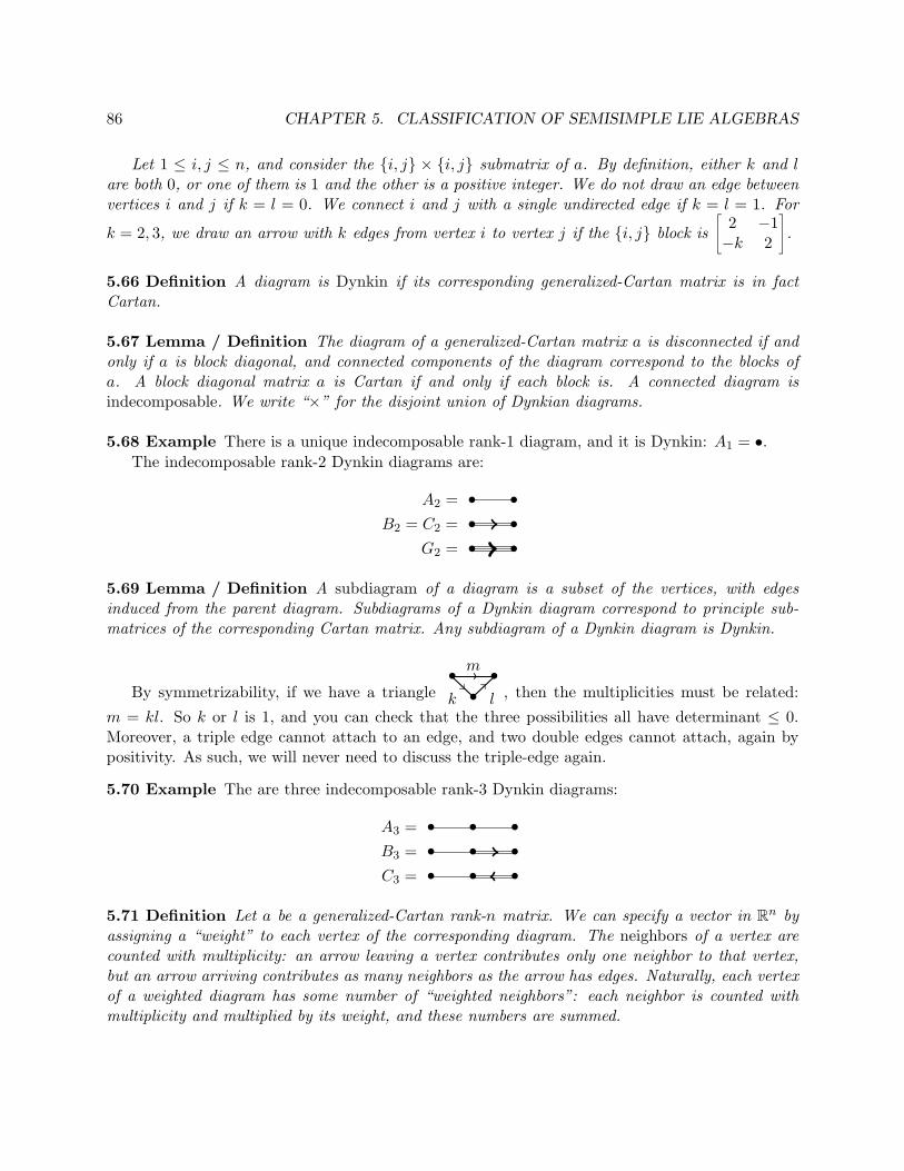
86 CHAPTER 5. CLASSIFICATION OF SEMISIMPLE LIE ALGEBRAS
Let 1 ≤ i, j ≤ n, and consider the {i, j} × {i, j} submatrix of a. By definition, either k and lare both 0, or one of them is 1 and the other is a positive integer. We do not draw an edge betweenvertices i and j if k = l = 0. We connect i and j with a single undirected edge if k = l = 1. For
k = 2, 3, we draw an arrow with k edges from vertex i to vertex j if the {i, j} block isñ
2 −1−k 2
ô.
5.66 Definition A diagram is Dynkin if its corresponding generalized-Cartan matrix is in factCartan.
5.67 Lemma / Definition The diagram of a generalized-Cartan matrix a is disconnected if andonly if a is block diagonal, and connected components of the diagram correspond to the blocks ofa. A block diagonal matrix a is Cartan if and only if each block is. A connected diagram isindecomposable. We write “×” for the disjoint union of Dynkian diagrams.
5.68 Example There is a unique indecomposable rank-1 diagram, and it is Dynkin: A1 = •.The indecomposable rank-2 Dynkin diagrams are:
A2 = • •B2 = C2 = • •
G2 = • •
5.69 Lemma / Definition A subdiagram of a diagram is a subset of the vertices, with edgesinduced from the parent diagram. Subdiagrams of a Dynkin diagram correspond to principle sub-matrices of the corresponding Cartan matrix. Any subdiagram of a Dynkin diagram is Dynkin.
By symmetrizability, if we have a triangle•k • l
•m
, then the multiplicities must be related:
m = kl. So k or l is 1, and you can check that the three possibilities all have determinant ≤ 0.Moreover, a triple edge cannot attach to an edge, and two double edges cannot attach, again bypositivity. As such, we will never need to discuss the triple-edge again.
5.70 Example The are three indecomposable rank-3 Dynkin diagrams:
A3 = • • •B3 = • • •C3 = • • •
5.71 Definition Let a be a generalized-Cartan rank-n matrix. We can specify a vector in Rn byassigning a “weight” to each vertex of the corresponding diagram. The neighbors of a vertex arecounted with multiplicity: an arrow leaving a vertex contributes only one neighbor to that vertex,but an arrow arriving contributes as many neighbors as the arrow has edges. Naturally, each vertexof a weighted diagram has some number of “weighted neighbors”: each neighbor is counted withmultiplicity and multiplied by its weight, and these numbers are summed.

5.5. CARTAN MATRICES AND DYNKIN DIAGRAMS 87
5.72 Lemma Let a be a generalized-Cartan matrix, and think of a vector ~x as a weighting of thecorresponding diagram. With the weighted-neighbor conventions in Definition 5.71, the multiplica-tion a~x can be achieved by subtracting the number of weighted neighbors of each vertex from twicethe weight of that vertex.
Thus, a generalized-Cartan matrix is singular if its corresponding diagram has a weighting suchthat each vertex has twice as many (weighted) neighbors as its own weight.
5.73 Corollary A ring of single edges, and hence any diagram with a ring as a subdiagram, is notDynkin.
Proof We assign weight 1 to each vertex; this shows that the determinant of the ring is 0:
·
•
•
••
•
•
• •· ·
·
1
1
11
1
1
11
· ·
a
( )= 0
�
5.74 Corollary The following diagrams correspond to singular matrices and hence are not Dynkin:
· · ·• • •
•
•
•
•
•
•
•
•
•
· · ·• • •
•
•
•
· · ·• • •
•
•
•
· · ·• • •• •

88 CHAPTER 5. CLASSIFICATION OF SEMISIMPLE LIE ALGEBRAS
· · ·• • •• •
· · ·• • •• •
• • • • •
• • • • •
Proof For example, we can show the last two as singular with the following weightings:
1 2 3 2 1
2 4 3 2 1 �
5.75 Lemma The following diagrams are not Dynkin:
•
• •
•det = −4
•
••
•
•det = −4
•
• •
•det = −8
•
• •
•not symmetrizable
5.76 Corollary The indecomposable Dynkin diagrams with double edges are the following:
Bn = • • · · · • •Cn = • • · · · • •F4 = • • • •
Proof Any indecomposable Dynkin diagram with a double edge is a chain. The double edge mustcome at the end of the chain, unless the diagram has rank 4. �
5.77 Lemma Consider a Y -shaped indecomposable diagram. Let the lengths of the three arms,including the middle vertex, be k, l,m. Then the diagram is Dynkin if and only if 1
k + 1l + 1
m > 1.
Proof One can show directly that the determinant of such a diagram is klm( 1k + 1
l + 1m − 1). We
present null-vectors for the three “Egyptian fraction” decompositions of 1 — triples k, l,m suchthat 1
k + 1l + 1
m = 1:
321
2 1
2 1 4
3 2
2
1
3 2 1
6
3
42 5 4 3 2 1 �

5.5. CARTAN MATRICES AND DYNKIN DIAGRAMS 89
5.78 Corollary The indecomposable Dynkin diagrams made entirely of single edges are:
An = • • · · · •
Dn = • • · · · •
•
•
E6 = • • •
•
• •
E7 = • • •
•
• • •
E8 = • • •
•
• • • •
All together, we have proven:
5.79 Theorem (Classification of indecomposable Dynkin diagrams) A diagram is Dynkinif and only if it is a disjoint union of indecomposable Dynkin diagrams. The indecomposable Dynkindiagrams comprise four infinite families and five “sporadic” cases:
An = • • · · · •
Dn = • • · · · •
•
•Bn = • • · · · • •Cn = • • · · · • •
E6 = • • •
•
• •
E7 = • • •
•
• • •
E8 = • • •
•
• • • •F4 = • • • •G2 = • •

90 CHAPTER 5. CLASSIFICATION OF SEMISIMPLE LIE ALGEBRAS
5.80 Example We mention the small-rank coindidences. We can continue the E series for smallern: E4 = A4, E5 = D5. E3 is not defined. The B, C, and D series make sense for n ≥ 2, whenceB2 = C2 and D2 = A1 × A1 and D3 = A3. Some diagrams have nontrivial symmetries: for n ≥ 1,the symmetry group of An has order 2, and similarly for Dn for n 6= 4. The diagram D4 has anunexpected symmetry: its symmetry group is S3, with order 6. The symmetry group of E6 isorder-2.
5.6 From Cartan Matrix to Lie Algebra
[8, Lectures 36 and 37]In Theorem 5.79, we classified indecomposable finite-type Cartan matrices, and therefore all
finite-type Cartan matrices. We can present generators and relations showing that each indecompos-able Cartan matrix is the Cartan matrix of some simple Lie algebra — indeed, the infinite familiesAn, Bn, Cn, and Dn correspond respectively to the classical Lie algebras sl(n,C), so(2n + 1,C),sp(n,C), and so(2n,C) — and it is straightforward to show that a disjoint union of Cartan matricescorresponds to a direct product of Lie algebras.
In this section, we explain how to construct a semisimple Lie algebra for any finite-type Cartanmatrix, and we show that a semisimple Lie algebra is determined by its Cartan matrix. Thiswill complete the proof of the classification of semisimple Lie algebras. Most, but not all, of theconstruction applies to generalized-Cartan matrices; the corresponding Lie algebras are Kac-Moody,which are infinite-dimensional versions of semisimple Lie algebras. We will not discuss Kac-Moodyalgebras here.
5.81 Lemma / Definition Let ∆ be a rank-n Dynkin diagram with vertices labeled a basis {α1, . . . , αn}of a vector space h∗, and let aij be the corresponding Cartan matrix. Since aij is nondegenerate, itdefines a map ∨ : h∗ → h by aij = 〈αj , α∨i 〉. We define g = g∆ to be the Lie algebra generated by{ei, fi, hi}ni=1 subject to the relations
[hi, ej ] = aijej (5.6.1)[hi, fj ] = −aijfj (5.6.2)[ei, fj ] = δijhi (5.6.3)[hi, hj ] = 0 (5.6.4)
For each i, we write sl(2)i for the subalgebra spanned by {ei, fi, hi}; clearly sl(2)i ∼= sl(2).Let Q = Z∆ be the root lattice of ∆. Then the free Lie algebra generated by {ei, fi, hi}ni=1 has a
natural Q-grading, by deg ei = αi, deg fi = −αi, and deg hi = 0; under this grading, the relationsare homogeneous, so the grading passes to the quotient g∆.
Let h ⊆ g be the subalgebra generated by {hi}ni=1; then it is abelian and spanned by {hi}ni=1. Theadjoint action ad : h y g is diagonalized by the grading: hi acts on anything of degree q ∈ Q by〈q, α∨i 〉.
Let n+ be the subalgebra of g generated by {ei}ni=1 and let n− be the subalgebra of g generatedby {fi}ni=1; the algebras n± are called the “upper-” and “lower-triangular” subalgebras.

5.6. FROM CARTAN MATRIX TO LIE ALGEBRA 91
5.82 Proposition Let ∆, g, h, n± be as in Lemma/Definition 5.81. Then g = n−⊕ h⊕ n+ as vectorspaces; this is the “triangular decomposition” of g.
Proof That n−, h, n+ intersect trivially follows form the grading, so it suffices to show that g =n− + h + n+. By inspecting the relations, we see that (ad fi)n− ⊆ n−, (ad fi)h ⊆ 〈fi〉 ⊆ n−, and(ad fi)n+ ⊆ h+ n+. Therefore ad fi preserves n−+ h+ n+, h does so obviously, and ad ei does so bythe obvious symmetry fi ↔ ei. Therefore n− + h + n+ is an ideal of g and therefore a subalgebra,but it contains all the generators of g. �
5.83 Proposition Let ∆, g be as in Lemma/Definition 5.81, and let λ ∈ h∗. Write C〈f1, . . . , fn〉for the free algebra generated by noncommuting symbols f1, . . . , fn and Mλ
def= C〈f1, . . . , fn〉vλ forits free module generated by the symbol vλ. Then there exists an action of g on Mλ such that:
fiÄ∏
fjkvλä
=Äfi∏
fjkävλ (5.6.5)
hiÄ∏
fjkvλä
=
(λ(hi)−
∑k
ai,jk
) Ä∏fjkvλ
ä(5.6.6)
eiÄ∏
fjkvλä
=∑
k s.t. jk=i
fj1 · · · fjk−1hifjk+1
· · · fjl vλ (5.6.7)
Proof We have only to check that the action satisfies the relations equations 5.6.1 to 5.6.4. TheQ-grading verifies equations 5.6.1, 5.6.2, and 5.6.4; we need only to check equation 5.6.3. Wheni 6= j, the action by ei ignores any action by fj , and so we need only check that [ei, fi] acts by hi.Write f for some monomial fj1 · · · fjn . Then eifi(fvλ) = ei(fifvλ) = hifvλ + fiei(fvλ), clear bythe construction. �
5.84 Definition The g-module Mλ defined in Proposition 5.83 is the Verma module of g withweight λ.
5.85 Corollary The map h → h is an isomorphism, so h ↪→ h. The upper- and lower-triangularalgebras n− and n+ are free on {fi} and {ei} respectively.
5.86 Proposition Assume that ∆ is an indecomposable system of simple roots, in the sense thatthe Dynkin diagram of the Cartan matrix of ∆ is connected. Construct g as in Lemma/Definition 5.81.Then any proper ideal of g is graded, contained in n− + n+, and does not contain any ei or fi.
Proof The grading on g is determined by the adjoint action of h = h. Let a be an ideal of g anda ∈ a. Let a =
∑aqgq where gq are homogeneous of degree q ∈ Q. Then [hi, a] =
∑〈q, α∨i 〉aqgq, andso [h, a] has the same dimension as the number of non-zero coefficients aq; in particular, gq ∈ [h, a].Thus a is graded.
Suppose that a has a degree-0 part, i.e. suppose that there is some h ∈ h∩ a. Since the Cartanmatrix a is nonsingular, there exists αi ∈ ∆ with αi(h) 6= 0. Then [fi, h] = αi(h)fi 6= 0, and sofi ∈ a.
Now let a be any ideal with fi ∈ a for some i. Then hi = [ei, fi] ∈ a and ei = −12 [ei, hi] ∈ a.
But let αj be any neighbor of αi in the Dynkin diagram. Then aij 6= 0, and so [fj , hi] = aijfj 6= 0;then fj ∈ a. Therefore, if the Dynkin diagram is connected, then any ideal of g that contains somefi (or some ei by symmetry) contains every generator of g. �

92 CHAPTER 5. CLASSIFICATION OF SEMISIMPLE LIE ALGEBRAS
5.87 Corollary Under the conditions of Proposition 5.86, g has a unique maximal proper ideal.
Proof Let a and b be any two proper ideals of g. Then the ideal a + b does not contain h or anyei or fi, and so is a proper ideal. �
5.88 Definition Let ∆ be a system of simple roots with connected Dynkin diagram, and let g = g∆
be defined as in Lemma/Definition 5.81. We define g = g∆ as the quotient of g by its uniquemaximal proper ideal. Then 〈hi, ei, fi〉 ↪→ g, where by 〈hi, ei, fi〉 we mean the linear span of thegenerators of g. Since we quotiented by a maximal ideal, g is simple.
5.89 Theorem (Serre Relations) Let g be as in Definition 5.88, and ei, fi the images of thecorresponding generators of g. Then:
(ad ej)1−ajiei = 0 (5.6.8)
(ad fj)1−ajifi = 0 (5.6.9)
Proof We will check equation 5.6.9; equation 5.6.8 is exactly analogous. Let s be the left-hand-sideof equation 5.6.9, interpreted as an element of g. We will show that the ideal generated by s isproper.
When i = j, s = 0, and when i 6= j, aji ≤ 0, and so the degree of s is −αi − (≥ 1)αj . Inparticular, bracketing with fk and hk only moves the degree further from 0. Therefore, the claimfollows from the following equation:
[ek, s]g = 0 for any k (5.6.10)
When k 6= i, j, [ek, fi] = [ek, fj ] = 0. So it suffices to check equation 5.6.10 when k = i, j. Letm = −aji. When k = j, we compute:
(ad ej)(ad fj)1+mfi =îad ej , (ad fj)1+m
ófi + (ad fj)1+m(ad ej)fi (5.6.11)
=îad ej , (ad fj)1+m
ófi + 0 (5.6.12)
=m∑l=0
(ad fj)m−lÄad[ej , fj ]
ä(ad fj)lfi (5.6.13)
=m∑l=0
(ad fj)m−l(adhj)(ad fj)lfi (5.6.14)
=m∑l=0
Äl(−〈αj , α∨j 〉)− 〈αi, α∨j 〉
ä(ad fj)mfi (5.6.15)
=
(m∑l=0
Ä−2l +m
ä)(ad fj)mfi (5.6.16)
=Ç−2
m(m+ 1)2
+ (m+ 1)må
(ad fj)mfi = 0 (5.6.17)
where equation 5.6.12 follows by [ei, fj ] = 0, equation 5.6.13 by the fact that ad is a Lie algebrahomomorphism, and the rest is equations 5.6.2 and 5.6.3, that m = −aji, and arithmetic.
5.6. FROM CARTAN MATRIX TO LIE ALGEBRA 93
When k = i, ei and fj commute, and we have:
(ad ei)(ad fj)1+mfi =îad ej , (ad fj)1+m
ófi + (ad fj)1+m(ad ei)fi (5.6.18)
= 0 + (ad fj)1+m(ad ei)fi (5.6.19)
= (ad fj)1+mhi = 0 (5.6.20)
provided that m ≥ 1. When m = 0, we use the symmetrizability of the Cartan matrix: if aji = 0then aij = 0. Therefore
(ad ei)(ad fj)1−ajifi = (ad ei)[fj , fi] = −(ad ei)(ad fi)1−aijfj (5.6.21)
which vanishes by the first computation. �
We have defined for each indecomposable Dynkin diagram ∆ a simple Lie algebra g∆. If∆ = ∆1 ×∆2 is a disjoint union of Dynkin diagrams, we define g∆
def= g∆1 × g∆2 .
5.90 Definition Let V be a (possibly-infinite-dimensional) g-module. An element v ∈ V is inte-grable if for each i, the sl(2)i-submodule of V generated by v is finite-dimensional. We write I(V )for the set of integrable elements of V .
5.91 Lemma Let V be a g-module. Then I(V ) is a g-submodule.
Proof Let N ⊆ V be an (n + 1)-dimensional irreducible representation of sl(2)i; then it is iso-morphic to Vn defined in Example 5.17. It suffices to show that ejN is contained within somefinite-dimensional sl(2)i submodule of V for i 6= j; the rest follows by switching e ↔ f and per-muting the indices, using the fact that {ej , fj} generate g.
Then N is spanned by {fikv0}nk=0 where v0 ∈ N is the vector annihilated by ei; in particular,fin+1v0 = 0. Since ej and fi commute, ejN is spanned by {fikejv0}nk=0. It suffices to compute
the sl(2)i module generated by ejv0, or at least to show that it is finite-dimensional. The actionof hi on ejv0 is hiejv0 = ([hi, ej ] + ejhi)v0 = (aij + n)ejv0. For k 6= n + 1, fki ejv0 = ejf
ki v0 = 0.
Moreover, by Theorem 5.89, eki ejv0 = [eki , ej ]v0 + ejeki v0 = (ad ei)k(ej)v0 + 0, which vanishes for
large enough k. Then the result follows by Theorem 3.24 and the fact that [ei, fi] = hi. �
5.92 Corollary Let ∆ be a Dynkin diagram and define g as above. Then g is ad-integrable.
Proof Since {ek, fk} generate g, it suffices to show that ek and fk are ad-integrable for each k.But the sl(2)i-module generated by fk has fk as its highest-weight vector, since [ei, fk] = 0, and isfinite-dimensional, since (ad fi)nfk = 0 for large enough n by Theorem 5.89. �
5.93 Corollary The non-zero weights R of ad : g y g form a root system.
Proof Axioms RS1, RS2, RS3, RS4, and Nondeg of Definition 5.46 follow from the ad-integrability. Axiom Reduced and that R is finite follow from Lemma 5.57. �
5.94 Theorem (Classification of finite-dimensional simple Lie algebras) The list given inTheorem 5.79 classifies the finite-dimensional simple Lie algebras over C.

94 CHAPTER 5. CLASSIFICATION OF SEMISIMPLE LIE ALGEBRAS
Proof A Lie algebra with an indecomposable root system is simple, because any such system hasa highest root, and linear combination of roots generates the highest root, and the highest rootgenerates the entire algebra. So it suffices to show that two simple Lie algebras with isomorphicroot systems are isomorphic.
Let ∆ be an indecomposable root system, and define g and g as above. Let g1 be a Lie algebrawith root system ∆. Then the relations defining g hold in g1, and so there is a surjection g� g1; ifg1 is simple, then the kernel of this surjection is a maximal ideal of g. But g has a unique maximalideal, and g is the quotient by this ideal; thus g1
∼= g. �
5.95 Example The families ABCD correspond to the classical Lie algebras: An ↔ sl(n + 1),Bn ↔ so(2n+ 1), Cn ↔ sp(n), and Dn ↔ so(2n). We recall that we have defined sp(n) as the Liealgebra that fixes the nondegenerate antisymmetric 2n × 2n bilinear form: sp(n) ⊆ gl(2n). TheEFG Lie algebras are new.
The coincidences in Example 5.80 correspond to coincidences of classical Lie algebras: so(6) ∼=sl(4), so(5) ∼= sp(2), and so(4) ∼= sl(2) × sl(2). The identity so(3) ∼= sl(2) suggests that we defineB1 = A1 = •, but sl(2) is not congruent to sp(1) or to so(2), so we do not assign meaning to C1 orD1, and justifying the name B1 for • but not C1 is ad hoc.
Exercises
1. (a) Show that SL(2,R) is topologically the product of a circle and two copies of R, hence itis not simply connected.
(b) Let S be the simply connected cover of SL(2,R). Show that its finite-dimensional com-plex representations, i.e., real Lie group homomorphisms S → GL(n,C), are determinedby corresponding complex representations of the Lie algebra Lie(S)C = sl(2,C), andhence factor through SL(2,R). Thus S is a simply connected real Lie group with nofaithful finite-dimensional representation.
2. (a) Let U be the group of 3 × 3 upper-unitriangular complex matrices. Let Γ ⊆ U be thecyclic subgroup of matrices 1 0 m
0 1 00 0 1
,where m ∈ Z. Show that G = U/Γ is a (non-simply-connected) complex Lie group thathas no faithful finite-dimensional representation.
(b) Adapt the solution to Set 4, Problem 2(b) to construct a faithful, irreducible infinite-dimensional linear representation V of G.
3. Following the outline below, prove that if h ⊆ gl(n,C) is a real Lie subalgebra with theproperty that every X ∈ h is diagonalizable and has purely imaginary eigenvalues, then thecorresponding connected Lie subgroup H ⊆ GL(n,C) has compact closure (this completesthe solution to Set 1, Problem 7).
(a) Show that adX is diagonalizable with imaginary eigenvalues for every X ∈ h.

5.6. FROM CARTAN MATRIX TO LIE ALGEBRA 95
(b) Show that the Killing form of h is negative semidefinite and its radical is the center ofh. Deduce that h is reductive and the Killing form of its semi-simple part is negativedefinite. Hence the Lie subgroup corresponding to the semi-simple part is compact.
(c) Show that the Lie subgroup corresponding to the center of h is a dense subgroup of acompact torus. Deduce that the closure of H is compact.
(d) Show that H is compact — that is, closed — if and only if it further holds that thecenter of h is spanned by matrices whose eigenvalues are rational multiples of i.
4. Let Vn = Sn(C2) be the (n+ 1)-dimensional irreducible representation of sl(2,C).
(a) Show that for m ≤ n, Vm ⊗ Vn ∼= Vn−m ⊕ Vn−m+2 ⊕ · · · ⊕ Vn+m, and deduce that thedecomposition into irreducibles is unique.
(b) Show that in any decomposition of V ⊗n1 into irreducibles, the multiplicity of Vn is equalto 1, the multiplicity of Vn−2k is equal to
(nk
)−( nk−1
)for k = 1, . . . , bn/2c, and all other
irreducibles Vm have multiplicity zero.
5. Let a be a symmetric Cartan matrix, i.e. a is symmetric with diagonal entries 2 and off-diagonal entries 0 or −1. Let Γ be a subgroup of the automorphism group of the Dynkindiagram D of a, such that every edge of D has its endpoints in distinct Γ orbits. Define thefolding D′ of D to be the diagram with a node for every Γ orbit I of nodes in D, with edgeweight k from I to J if each node of I is adjacent in D to k nodes of J . Denote by a′ theCartan matrix with diagram D′.
(a) Show that a′ is symmetrizable and that every symmetrizable generalized Cartan matrix(not assumed to be of finite type) can be obtained by folding from a symmetric one.
(b) Show that every folding of a finite type symmetric Cartan matrix is of finite type.
(c) Verify that every non-symmetric finite type Cartan matrix is obtained by folding froma unique symmetric finite type Cartan matrix.
6. An indecomposable symmetrizable generalized Cartan matrix a is said to be of affine type ifdet(a) = 0 and all the proper principal minors of a are positive.
(a) Classify the affine Cartan matrices.
(b) Show that every non-symmetric affine Cartan matrix is a folding, as in the previousproblem, of a symmetric one.
(c) Let h be a vector space, αi ∈ h∗ and α∨i ∈ h vectors such that a is the matrix 〈αj , α∨i 〉.Assume that this realization is non-degenerate in the sense that the vectors αi are linearlyindependent. Define the affine Weyl group W to be generated by the reflections sαi , asusual. Show that W is isomorphic to the semidirect product W0 nQ where Q and W0
are the root lattice and Weyl group of a unique finite root system, and that every suchW0 nQ occurs as an affine Weyl group.
(d) Show that the affine and finite root systems related as in (c) have the property that theaffine Dynkin diagram is obtained by adding a node to the finite one, in a unique way ifthe finite Cartan matrix is symmetric.

96 CHAPTER 5. CLASSIFICATION OF SEMISIMPLE LIE ALGEBRAS
7. Work out the root systems of the orthogonal Lie algebras so(m,C) explicitly, thereby verifyingthat they correspond to the Dynkin diagrams Bn if m = 2n + 1, or Dn if m = 2n. Deducethe isomorphisms so(4,C) ∼= sl(2,C)× sl(2,C), so(5,C) ∼= sp(4,C), and so(6,C) ∼= sl(4,C).
8. Show that the Weyl group of type Bn or Cn (they are the same because these two rootsystems are dual to each other) is the group Sn n (Z/2Z)n of signed permutations, and thatthe Weyl group of type Dn is its subgroup of index two consisting of signed permutationswith an even number of sign changes, i.e., the semidirect factor (Z/2Z)n is replaced by thekernel of Sn-invariant summation homomorphism (Z/2Z)n → Z/2Z
9. Let (h, R,R∨) be a finite root system, ∆ = {α1, . . . , αn} the set of simple roots with respectto a choice of positive roots R+, si = sαi the corresponding generators of the Weyl group W .Given w ∈W , let l(w) denote the minimum length of an expression for w as a product of thegenerators si.
(a) If w = si1 . . . sir and w(αj) ∈ R−, show that for some k we have αik = sik+1. . . sir(αj),
and hence siksik+1. . . sir = sik+1
. . . sirsj . Deduce that l(wsj) = l(w)− 1 if w(αj) ∈ R−.
(b) Using the fact that the conclusion of (a) also holds for v = wsj , deduce that l(wsj) =l(w) + 1 if w(αj) 6∈ R−.
(c) Conclude that l(w) = |w(R+) ∪ R−| for all w ∈ W . Characterize l(w) in more explicitterms in the case of the Weyl groups of type A and B/C.
(d) Assuming that h is over R, show that the dominant cone X = {λ ∈ h : 〈λ, α∨i 〉 ≥0 for all i} is a fundamental domain for W , i.e., every vector in h has a unique elementof X in its W orbit.
(e) Deduce that |W | is equal to the number of connected regions into which h is separatedby the removal of all the root hyperplanes 〈λ, α∨〉, α∨ ∈ R∨.
10. Let h1, . . . , hr be linear forms in variables x1, . . . , xn with integer coefficients. Let Fq denotethe finite field with q = pe elements. Prove that except in a finite number of “bad” charac-teristics p, the number of vectors v ∈ Fnq such that hi(v) = 0 for all i is given for all q by apolynomial χ(q) in q with integer coefficients, and that (−1)nχ(−1) is equal to the numberof connected regions into which Rn is separated by the removal of all the hyperplanes hi = 0.
Pick your favorite finite root system and verify that in the case where the hi are the roothyperplanes, the polynomial χ(q) factors as (q − e1) . . . (q − en) for some positive integers eicalled the exponents of the root system. In particular, verify that the sum of the exponentsis the number of positive roots, and that (by Problem 9(e)) the order of the Weyl group is∏i(1 + ei)
11. The height of a positive root α is the sum of the coefficients ci in its expansion α =∑i ciαi
on the basis of simple roots.
Pick your favorite root system and verify that for each k ≥ 1, the number of roots of heightk is equal to the number of the exponents ei in Problem 10 for which ei ≥ k.

5.6. FROM CARTAN MATRIX TO LIE ALGEBRA 97
12. Pick your favorite root system and verify that if h denotes the height of the highest rootplus one, then the number of roots is equal to h times the rank. This number h is calledthe Coxeter number. Verify that, moreover, the multiset of exponents (see Problem 10) isinvariant with respect to the symmetry ei 7→ h− ei.
13. A Coxeter element in the Weyl group W is the product of all the simple reflections, once each,in any order. Prove that a Coxeter element is unique up to conjugacy. Pick your favoriteroot system and verify that the order of a Coxeter element is equal to the Coxeter number(see Problem 12).
14. The fundamental weights λi are defined to be the basis of the weight lattice P dual to thebasis of simple coroots in Q∨, i.e., 〈λi, α∨j 〉 = δij .
(a) Prove that the stabilizer in W of λi is the Weyl group of the root system whose Dynkindiagram is obtained by deleting node i of the original Dynkin diagram.
(b) Show that each of the root systems E6, E7, and E8 has the property that its highest rootis a fundamental weight. Deduce that the order of the Weyl group W (Ek) in each caseis equal to the number of roots times the order of the Weyl group W (Ek−1), or W (D5)for k = 6. Use this to calculate the orders of these Weyl groups.
15. Let e1, . . . , e8 be the usual orthonormal basis of coordinate vectors in Euclidean space R8. Theroot system of type E8 can be realized in R8 with simple roots αi = ei − ei+1 for i = 1, . . . , 7and
α8 =Å−1
2,−1
2,−1
2,12,12,12,12,12
ã.
Show that the root lattice Q is equal to the weight lattice P , and that in this realization, Qconsists of all vectors β ∈ Z8 such that
∑i βi is even and all vectors β ∈
Ä12 ,
12 ,
12 ,
12 ,
12 ,
12 ,
12 ,
12
ä+
Z8 such that∑i βi is odd. Show that the root system consists of all vectors of squared length
2 in Q, namely, the vectors ±ei ± ej for i < j, and all vectors with coordinates ±12 and an
odd number of coordinates with each sign.
16. Show that the root system of type F4 has 24 long roots and 24 short roots, and that the rootsof each length form a root system of type D4. Show that the highest root and the highestshort root are the fundamental weights at the end nodes of the diagram. Then use Problem14(a) to calculate the order of the Weyl group W (F4). Show that W (F4) acts on the set ofshort (resp. long roots) as the semidirect product S3 nW (D4), where the symmetric groupS3 on three letters acts on W (D4) as the automorphism group of its Dynkin diagram.
17. Pick your favorite root system and verify that the generating function W (t) =∑w∈W tl(w) is
equal to∏i (1 + t+ · · ·+ tei), where ei are the exponents as in Problem 10.
18. Let S be the subring of W -invariant elements in the ring of polynomial functions on h. Pickyour favorite root system and verify that S is a polynomial ring generated by homogeneousgenerators of degrees ei + 1, where ei are the exponents as in Problem 10.

98 CHAPTER 5. CLASSIFICATION OF SEMISIMPLE LIE ALGEBRAS

Chapter 6
Representation Theory of SemisimpleLie Groups
6.1 Irreducible Lie-algebra representations
[8, Lectures 38 and 39] [18, Lectures 18 and 19]1
Any representation of a Lie group induces a representation of its Lie algebra, so we start our storythere. We recall Theorem 4.78: any finite-dimensional representation of a semisimple Lie algebra isthe direct sum of simple representations. In section 5.2 we computed the finite-dimensional simplerepresentations of sl(2); we now generalize that theory to arbitrary finite-dimensional semisimpleLie algebras.
6.1 Lemma / Definition Let g be a semisimple Lie algebra with Cartan subalgebra h and rootsystem R, and choose a system of positive roots R+. Let n± =
⊕α∈R± gα be the upper- and lower-
triangular subalgebras; then g = n− ⊕ h⊕ n+ as a a vector space. We define the Borel subalgebrab = h⊕ n+, and n+ is an ideal of b with h = b/n+.
Pick λ ∈ h∗; then b has a one-dimensional module Cvλ, where hvλ = λ(h) vλ for h ∈ h andn+vλ = 0.
As a subalgebra, b acts on g from the right, and so we define the Verma module of g with weightλ by:
Mλdef= Ug⊗Ub Cvλ (6.1.1)
As a vector space, Mλ∼= Un− ⊗C Cvλ. It is generated as a g-module by vλ with the relations
hvλ = λ(h)vλ, n+vλ = 0, and no relations on the action of n− except those from g.
Proof The explicit description of Mλ follows from Theorem 3.24: Ug = Un−⊗Uh⊗Un+ as vectorspaces. �
1I was absent for Lecture 39 in Mark Haiman’s class, and so those notes are missing from [8]. To prepare thisdocument, I thus turned to [18] for the proof of the Weyl Character Formula (Theorem 6.15). The presentation of thismaterial there is quite good, although differs from the presentation in [8]; in particular, [18] includes more motivationand examples, and discusses ch (Definition 6.10) in terms of group characters of the corresponding simply-connectedLie group. See also Footnote 1 in [18, page 106].
99

100 CHAPTER 6. REPRESENTATION THEORY OF SEMISIMPLE LIE GROUPS
6.2 Corollary Any module with highest weight λ is a quotient of Mλ.
6.3 Lemma Let ∆ = {α1, . . . , αn} be the simple roots of g, and let Q def= Z∆ be the root latticeand Q+
def= Z≥0∆. Then the weight grading given by the action of h on the Verma module Mλ is:
Mλ =⊕β∈Q+
(Mλ)λ−β (6.1.2)
Moreover, let N ⊆Mλ be a proper submodule. Then N ⊆⊕β∈Q+r{0} (Mλ)λ−β.
Proof The description of the weight grading follows directly from the description of Mλ givenin Lemma/Definition 6.1. Any submodule is graded by the action of h. Since (Mλ)λ = Cvλ isone-dimensional and generates Mλ, a proper submodule cannot intersect (Mλ)λ. �
6.4 Corollary For any λ ∈ h∗, the Verma module Mλ has a unique maximal proper submodule.The quotient Mλ � Lλ is an irreducible g-module. Conversely, any irreducible g-module withhighest weight λ is isomorphic to Lλ, since it must be a quotient of Mλ by a maximal ideal.
6.5 Definition Let g be a semisimple Lie algebra and ∆ = {α1, . . . , αn}. We recall the root latticeQ
def= Z∆ and the weight lattice P def= {λ ∈ h∗ s.t. 〈λ,Q∨〉 ⊆ Z}. A dominant integral weight is anelement of P+
def= {λ ∈ P s.t. 〈λ, α∨i 〉 ≥ 0 ∀i}.
We recall Definition 5.90.
6.6 Proposition If λ ∈ P+, then Lλ consists of integrable elements.
Proof Since Lλ is irreducible, its submodule of integrable elements is either 0 or the whole module.So it suffices to show that if λ ∈ P+, then vλ is integrable. Pick a simple root αi. By construction,eivλ = 0 and hivλ = 〈λ, α∨i 〉vλ. Since λ ∈ P+, 〈λ, α∨i 〉 = m ≥ 0 is an integer. Consider the sl(2)i-submodule of Mλ generated by vλ; if m is a nonnegative integer, from the representation theoryof sl(2) we know that eifm+1
i vλ = 0. But if j 6= i, then ejfm+1i vλ = fm+1
i ejvλ = 0. Recalling thegrading, we see then that fm+1
i vλ generates a submodule of Mλ, and so fm+1i vλ 7→ 0 in Lλ. Hence
the sl(2)i-submodule of Lλ generated by vλ is finite, and so vλ is integrable. �
6.7 Definition Let g be a semisimple Lie algebra. We define the category O to be a full subcategoryof the category g-mod of (possibly-infinite-dimensional) g modules. The objects X ∈ O are requiredto satisfy the following conditions:
• The action h y X is diagonalizable.
• For each λ ∈ h∗, the weight space Xλ is finite-dimensional.
• There exists a finite set S ⊆ h∗ such that the weights of X lie in S + (−Q+).
6.8 Lemma The category O is closed under submodules, quotients, extensions, and tensor prod-ucts.
6.1. IRREDUCIBLE LIE-ALGEBRA REPRESENTATIONS 101
Proof The h-action grades subquotients of any graded module, and acts diagonally. An extensionof graded modules is graded, with graded components extensions of the corresponding gradedcomponents. Since g is semisimple, any extension of finite-dimensional modules is a direct sum,and so the h-action is diagonal on any extension of objects in O. Finally, tensor products arehandled by Lemma 5.23. �
6.9 Definition Write the additive group h∗ multiplicatively: λ 7→ xλ. The group algebra Z[h∗] isthe algebra of “polynomials”
∑cix
λi, with the obvious addition and multiplication. I.e. Z[h∗] is thefree abelian group
⊕λ∈h∗ Zxλ, with multiplication given on a basis by xλxµ = xλ+µ.
Let Z[−Q+] be the subalgebra of Z[h∗] generated by {xλ s.t. − λ ∈ Q+}. This has a naturaltopology given by setting ‖x−αi‖ = c−αi for αi a simple root and c some real constant with c > 1.We let Z[[−Q+]] be the completion of Z[−Q+] with respect to this topology. Equivalently, Z[[−Q+]]is the algebra of formal power series in the variables x−α1 , . . . , x−αn with integer coefficients.
Then Z[−Q+] is a subalgebra of both Z[h∗] and Z[[−Q+]]. We will write Z[h∗,−Q+]] for thealgebra Z[h∗]⊗Z[−Q+] Z[[−Q+]].
The algebra Z[h∗,−Q+]] is a formal gadget, consisting of formal fractional Laurant series. We useit as a space of generating functions.
6.10 Definition Let X ∈ O. We define ch(X) ∈ Z[h∗,−Q+]] by:
ch(X) def=∑
λ a weight of X
dim(Xλ)xλ (6.1.3)
We remark that every coefficient of ch(X) is a nonnegative integer, and if Y is a subquotient
6.11 Example Let Mλ be the Verma module with weight λ, and let R+ be the set of positiveroots of g. Then
ch(Mλ) =xλ∏
α∈R+(1− x−α)
def= xλ∏α∈R+
∞∑l=0
x−lα (6.1.4)
This follows from Theorem 3.24, the explicit description of Mλ∼= Un−⊗Cvλ, and some elementary
combinatorics.
6.12 Proposition Let g be simple Lie algebra, P+ the set of dominant integral weights, and Wthe Weyl group. Let λ ∈ P+, and Lλ the irreducible quotient of Mλ given in Corollary 6.4. Then:
1. ch(Lλ) is W -invariant.
2. If µ is a weight of Lλ, then µ ∈W (ν) for some ν ∈ P+ ∩ (λ−Q+).
3. Lλ is finite-dimensional.
Conversely, every finite-dimensional irreducible g-module is Lλ for a unique λ ∈ P+.
Proof 1. We use Proposition 6.6: Lλ consists of integrable elements. Let αi be a root ofg; then Lλ splits as an sl(2)i module: Lλ =
⊕Va, where each Va is an irreducible sl(2)i

102 CHAPTER 6. REPRESENTATION THEORY OF SEMISIMPLE LIE GROUPS
submodule. In particular, Va = Cva,m ⊕ Cva,m−2 · · · ⊕ Cva,−m for some m depending on a,where hi acts on Cva,l by l. But ch(Lλ) =
∑a ch(Va) =
∑a∑j=−m,−m+2,...,m ch(Cva,m). Let
chÄC(va)l
ä= xµa,l ; then 〈µa,l, α∨i 〉 = l by definition, and va,l−2 ∈ fiCva,l, and so siµa,l = µa,−l.
This shows that ch(Va) is fixed under the action of si, and so ch(Lλ) is also si-invariant. Butthe reflections si generate W , and so ch(Lλ) is W -invariant.
2. We partially order P : ν ≤ µ if µ− ν ∈ Q+. In particular, the weights of Lλ are all less thanor equal to λ.
Let λ ∈ P . Then si(λ) = λ−〈λ, α∨i 〉αi, and so W (λ) ⊆ λ+Q. If λ ∈ P+ then 〈λ, α∨i 〉 ≥ 0 forevery i and so si ≤ λ; if λ ∈ P r P+ then there is some i with 〈λ, α∨i 〉 < 0, i.e. some i withsi(λ) > λ. But W is finite, so for any λ ∈ P , W (λ) has a maximal element, which must bein P+. This proves that P = W (P+).
Thus, if µ is a weight of Lλ, then µ ∈W (ν) for some ν ∈ P+. But by 1., ν is a weight of Lλ,and so ν ≤ λ. This proves statements 2.
Moreover, the W -invariance of ch(Lλ) shows that if λ ∈ P+, then W (λ) ⊆ λ − Q+, andmoreover that P+ is a fundamental domain of W .
3. The Weyl group W is finite. Consider the two cones R≥0P+ and −R≥0Q+. Since the innerproduct (the symmetrization of the Cartan matrix) is positive definite and by constructionthe inner product of anything in R≥0P+ with anything in −R≥0Q+ is negative, the two conesintersect only at 0. Thus there is a hyperplane separating the cones: i.e. there exists a linearfunctional η : h∗R → R such that its value is positive on P+ but negative on −Q+. Thenλ−Q+ is below the η = η(λ) hyperplane. But −Q+ is generated by −αi, each of which hasa negative value under η, and so λ−Q+ contains only finitely many points µ with η(µ) ≥ 0.Thus P+ ∩ (λ−Q+) is finite, and hence so is its image under W .
For the converse statement, let L be a finite-dimensional irreducible g-module, and let v ∈ Lbe any vector. Then consider n+v, the image of v under repeated application of various eis. Byfinite-dimensionality, n+v must contain a vector l ∈ n+v so that eil = 0 for every i. By the sl(2)representation theory, l must be homogeneous, and indeed a top-weight vector of L, and by theirreducibility l generates L. Let the weight of l be λ; then the map vλ → l generates a map Mλ � L.But Mλ has a unique maximal submodule, and since L is irreducible, this maximal submodule mustbe the kernel of the map Mλ � L. Thus L ∼= Lλ. �
6.13 Lemma / Definition Let g be a semisimple Lie algebra, h its Cartan subalgebra, and ∆ ={α1, . . . , αn} its simple root system. For each i = 1, . . . , n, we define a fundamental weight Λi ∈ h∗
by 〈Λi, α∨j 〉 = δij. Then P+ = Z≥0{Λ1, . . . ,Λn}.The following are equivalent, and define the Weyl vector ρ:
1. ρ =∑ni=1 Λi. I.e. 〈ρ, α∨j 〉 = 1 for every j.
2. ρ = 12
∑α∈R+
α.
Proof Let ρ2 = 12
∑α∈R+
α. Since si(R+r{αi}) = R+ but si(αi) = −αi, we see that si(ρ) = ρ−αi,and so 〈ρ, α∨i 〉 = 1 for every i. The rest is elementary linear algebra. �

6.1. IRREDUCIBLE LIE-ALGEBRA REPRESENTATIONS 103
6.14 Definition Let λ ∈ P+. We define the character χλ of λ to be ch(Lλ).
6.15 Theorem (Weyl Character Formula) Let ε : W → {±1} be given by ε(w) = dethw; i.e.ε is the group homomorphism generated by si 7→ −1 for each i. Let λ ∈ P+. Then χλ can becomputed as follows:
χλ =
∑w∈W
ε(w)xw(λ+ρ)−ρ
∏α∈R+
(1− x−α)=
∑w∈W
ε(w)xw(λ+ρ)
∏α∈R+
(xα/2 − x−α/2)(6.1.5)
The equality of fractions follows simply from the description ρ = 12
∑α∈R+
α.
6.16 Remark The sum in equation 6.1.5 is finite.Indeed, the numerator and denominator on the right-hand-side fraction are obiously antisym-
metric in W , and so the whole expression is W -invariant. The numerator on the left-hand-side frac-tion is a polynomial, and each (1− x−α) is invertible as a power series: (1− x−α)−1 =
∑∞n=0 x
−nα.So the fraction is a W -invariant power series, and hence a polynomial.
To prove Theorem 6.15 we will need a number of lemmas. In Example 6.11 we computed thecharacter of the Verma module Mλ. Then Theorem 6.15 asserts that:
ch(Lλ) =∑w∈W
ε(w) chÄMw(λ+ρ)−ρ
ä(6.1.6)
As such, we will begin by understanding Mλ better. We recall Lemma/Definition 4.65: Let (, ) bethe Killing form on g, and {xi} any basis of g with dual basis {yj}, i.e. (xi, yj) = δij for every i, j;then c =
∑xiyi ∈ Ug is central, and does not depend on the choice of basis.
6.17 Lemma Let λ ∈ h∗ and Mλ the Verma module with weight λ. Let c ∈ Ug be the Casimir,corresponding to the Killing form on g. Then c acts on Mλ by multiplication by (λ, λ+ 2ρ).
Proof Let g have rank n. Write R for the set of roots of g, R+ for the positive roots, and ∆ forthe simple roots, as we have previously.
Recall Lemma 5.37. We construct a basis of g as follows: we pick an orthonormal basis {ui}ni=1
of h. For each α a non-zero root of g, the space gα is one-dimensional; let xα be a basis vector ingα. Then the dual basis to {ui}ni=1 ∪ {xα}α∈Rr{0} is {ui}ni=1 ∪ {yα}α∈Rr{0}, where yα = x−α
(xα,x−α) .Then:
c =n∑i=1
u2i +
∑α∈Rr{0}
xαyα =n∑i=1
u2i +
∑α∈Rr{0}
xαx−α(xα, x−α)
=n∑i=1
u2i +
∑α∈R+
xαx−α + x−αxα(xα, x−α)
(6.1.7)
Since Mλ is generated by its highest weight vector vλ, and c is central, to understand the actionof c on Mλ it suffices to compute cvλ. We use the fact that for α ∈ R+, xαvλ = 0; then
xαx−αvλ = hαvλ + x−αxαvλ = hαvλ = λ(hα) vλ (6.1.8)

104 CHAPTER 6. REPRESENTATION THEORY OF SEMISIMPLE LIE GROUPS
where for each α ∈ R+ we have defines hα ∈ h by hα = [xα, x−α]. Moreover, (, ) is g-invariant, and[hα, xα] = α(hα)xα, where α(hα) 6= 0. So:
(xα, x−α) =1
α(hα)
Ä[hα, xα], x−α
ä=
1α(hα)
Ähα, [xα, x−α]
ä=
(hα, hα)α(hα)
(6.1.9)
We also have that uivλ = λ(ui)vλ, and since {ui} is an orthonormal basis, (λ, λ) =∑ni=1
Äλ(ui)
ä2.
Thus:
cvλ =n∑i=1
Äλ(ui)
ä2vλ +
∑α∈R+
λ(hα)(hα,hα)α(hα)
vλ =
Ñ(λ, λ) +
∑α∈R+
λ(hα)α(hα)(hα, hα)
évλ (6.1.10)
We recall that hα is proportional to α∨, that (α, α) = 4/(α∨, α∨), and that λ(α∨) = (λ, α)/(α, α).Then λ(hα)α(hα)
(hα,hα) = (λ, α), and so:
(λ, λ) +∑α∈R+
λ(hα)α(hα)(hα, hα)
= (λ, λ) +∑α∈R+
(λ, α) = (λ, λ+ 2ρ) (6.1.11)
Thus c acts on Mλ by multiplication by (λ, λ+ 2ρ). �
6.18 Lemma / Definition Let X be a g-module. We weight vector v ∈ X is singular if n+v = 0.In particular, any highest-weight vector is singular, and conversely any singular vector is the highestweight vector in the submodule it generates.
6.19 Corollary Let λ ∈ P , and Mλ the Verma module with weight λ. Then Mλ contains finitelymany singular vectors, in the sense that their span is finite-dimensional.
Proof Let Cλ be the set Cλ def= {µ ∈ P s.t. (µ+ ρ, µ+ ρ) = (λ+ ρ, λ+ ρ)}. Then Cλ is a spherein P centered at −ρ, and in particular it is a finite set. On the other hand, since (µ+ ρ, µ+ ρ) =(µ, µ+ 2ρ) + (ρ, ρ), we see that:
Cλ = {µ ∈ P s.t. c acts on Mµ by (λ, λ+ 2ρ)} (6.1.12)
Recall that any module with highest weight µ is a quotient of Mµ. Let v ∈ Mλ be a non-zerosingular vector with weight µ. Then on the one hand cv = (λ, λ+ 2ρ)v, since v ∈ Mλ, and on theother hand cv = (µ, µ+ 2ρ), since v is in a quotient of Mµ. In particular, µ ∈ Cλ. But the weightspaces (Mλ)µ of Mλ are finite-dimensional, and so the dimension of the space of singular vectors isat most
∑µ∈Cλ dim
Ä(Mλ)µ
ä<∞. �
6.20 Corollary Let λ ∈ P . Then there are nonnegative integers bλ,µ such that
chMλ =∑
bλ,µ chLµ (6.1.13)
and bλ,µ = 0 unless µ ≤ λ and µ ∈ Cλ. Moreover, bλ,λ = 0.
6.1. IRREDUCIBLE LIE-ALGEBRA REPRESENTATIONS 105
Proof We construct a filtration on Mλ. Since Mλ has only finitely many non-zero singular vectors,we choose w1 a singular vector of minimal weight µ1, and let F1Mλ be the submodule of Mλ
generated by w1. Then F1Mλ is irreducible with highest weight µ1. We proceed by induction,letting wi be a singular vector of minimal weight in Mλ/Fi−1Mλ, and FiMλ the primage of thesubrepresentation generated by wi. This filters Mλ:
0 = F0Mλ ⊆ F1Mλ ⊆ . . . (6.1.14)
Moreover, since Mλ has only finitely many weight vectors all together, the filtration must terminate:
0 = F0Mλ ⊆ F1Mλ ⊆ · · · ⊆ FkMλ = Mλ (6.1.15)
By construction, the quotients are all irreducible: FiMλ/Fi−1Mλ = Lµi for some µi ∈ Cλ, µi ≤ λ.We recall that ch is additive for extensions. Therefore
chMλ =k∑i=1
ch(FiMλ/Fi−1Mλ) =k∑i=1
chLµi (6.1.16)
Then bλ,µ is the multiplicity of µ appearing as the weight of a singular vector of Mλ, and we haveequation 6.1.13. The conditions stated about bλ,µ are immediate: we saw that µ can only appearas a weight of Mλ if µ ∈ Cλ and µ ≤ λ; moreover, Lλ appears as a subquotient of Mλ exactly once,so bλ,λ = 1. �
6.21 Definition The coefficients bλ,µ in equation 6.1.13 are the Kazhdan-Luztig multiplicities.
6.22 Lemma If λ ∈ P+, µ ≤ λ, µ ∈ Cλ, and µ+ ρ ≥ 0, then µ = λ.
Proof We have that (µ + ρ, µ + ρ) = (λ + ρ, λ + ρ) and that λ − µ =∑ni=1 kiαi, where all ki are
nonnegative. Then
0 = (λ+ ρ, λ+ ρ)− (µ+ ρ, µ+ ρ)
=Ä(λ+ ρ)− (µ+ ρ), (λ+ ρ) + (µ+ ρ)
ä= (λ− µ, λ+ µ+ 2ρ)
=n∑i=1
ki(α, λ+ µ+ 2ρ)
But λ, µ + ρ ≥ 0, and (αi, ρ) > 0, so (α, λ + µ + 2ρ) > 0, and so all ki = 0 since they arenonnegative. �
Proof (of Theorem 6.15) We have shown (Corollary 6.20) that chMλ =∑bλ,µ chLµ, were bλ,µ
is a lower-triangular matrix on Cλ = Cµ with ones on the diagonal. Thus it has a lower-triangularinverse with ones on the diagonal:
chLλ =∑
µ≤λ,µ∈Cλcλ,µ chMµ (6.1.17)

106 CHAPTER 6. REPRESENTATION THEORY OF SEMISIMPLE LIE GROUPS
But by equation 6.1.8 statement 1., chLλ is W -invariant, provided that λ ∈ P+, thus so is∑cλ,µ chMµ. We recall Example 6.11:
chMµ =xµ∏
α∈R+(1− x−α)
=xµ+ρ∏
α∈R+(xα/2 − x−α/2)
(6.1.18)
Therefore
chLλ =∑µ≤λ,µ∈Cλ cλ,µx
µ+ρ∏α∈R+
(xα/2 − x−α/2)(6.1.19)
But the denominator if W -antisymmetric, and so the numerator must be as well:∑µ≤λ,µ∈Cλ
cλ,µxw(µ+ρ) =
∑µ≤λ,µ∈Cλ
ε(w)cλ,µxµ+ρ for every w ∈W (6.1.20)
This is equivalent to the condition that cλ,µ = ε(w)cλ,w(µ+ρ)−ρ. By the proof of equation 6.1.8statement 2., we know that P+ is a fundamental domain of W ; since cλ,λ = 1, if µ+ ρ ∈W (λ+ ρ),then cλ,µ = ε(w), and so:
∑µ≤λ,µ∈Cλ
cλ,µxµ+ρ =
∑w∈W
áxw(λ+ρ) +
∑µ<λ,µ∈Cλµ+ρ∈P+
cλ,µxw(µ+ρ)
ë(6.1.21)
But the rightmost sum is empty by Lemma 6.22. �
6.23 Remark Specializing to the trivial representation L0, Theorem 6.15 says that
1 =∑w∈W ε(w)xw(ρ)∏
α∈R+(xα/2 − x−α/2)
(6.1.22)
So we can rewrite equation 6.1.5 as
χλ =∑w∈W ε(w)xw(λ+ρ)∑w∈W ε(w)xw(ρ)
(6.1.23)
The following is an important corollary:
6.24 Theorem (Weyl Dimension Formula) Let λ ∈ P+. Then dimLλ =∏α∈R+
(α, λ+ ρ)(α, ρ)
.
Proof The formula ch(Lλ) =∑
w∈W ε(w)xw(λ+ρ)∏α∈R+
(xα/2−x−α/2)is a polynomial in x. In particular, it defines a
real-valued function on R>0×h given by xα 7→ aα(h) — when a = 1 or h = 0, the formula as writtenis the indeterminate form 0
0 , but the function clearly returns∑µ dim
Ä(Lλ)µ
ä= dimLλ. We will
calculate this value of the function by taking a limit, using l’Hopital’s rule.

6.1. IRREDUCIBLE LIE-ALGEBRA REPRESENTATIONS 107
In particular, letting xα 7→ et(α,λ+ρ) in equation 6.1.22 gives∏α∈R+
Äet(α/2,λ+ρ) − e−t(α/2,λ+ρ)
ä=∑w∈W
ε(w)et(w(ρ),λ+ρ) =∑w∈W
ε(w)et(ρ,w(λ+ρ)) (6.1.24)
where the second equality comes from w 7→ w−1 and (w−1x, y) = (x,wy). On the other hand, welet xα 7→ et(α,ρ) in equation 6.1.5. Then
chLλ|x=etρ =∑w∈W ε(w)et(w(λ+ρ),ρ)∏
α∈R+
(et(α/2,ρ) − e−t(α/2,ρ)
) (6.1.25)
=∏α∈R+
Äet(α/2,λ+ρ) − e−t(α/2,λ+ρ)
ä∏α∈R+
(et(α/2,ρ) − e−t(α/2,ρ)
) (6.1.26)
=∏α∈R+
Äet(α/2,λ+ρ) − e−t(α/2,λ+ρ)
ä(et(α/2,ρ) − e−t(α/2,ρ)
) (6.1.27)
Therefore
dimLλ = limt→0
∏α∈R+
Äet(α/2,λ+ρ) − e−t(α/2,λ+ρ)
ä(et(α/2,ρ) − e−t(α/2,ρ)
) (6.1.28)
=∏α∈R+
limt→0
Äet(α/2,λ+ρ) − e−t(α/2,λ+ρ)
ä(et(α/2,ρ) − e−t(α/2,ρ)
) (6.1.29)
l’H=∏α∈R+
limt→0
Ä(α/2, λ+ ρ)et(α/2,λ+ρ) + (α/2, λ+ ρ)e−t(α/2,λ+ρ)
ä((α/2, ρ)et(α/2,ρ) + (α/2, ρ)e−t(α/2,ρ)
) (6.1.30)
=∏α∈R+
(α, λ+ ρ)(α, ρ)
(6.1.31)�
6.25 Example Let us compute the dimensions of the irreducible representations of g = sl(n+ 1).We work with the standard the simple roots be ∆ = {α1, . . . , αn}, whence R+ = {αi +αi+1 + · · ·+αj}1≤i<j≤n. Let us write λ and ρ in terms of the fundamental weights Λi, defined by (Λi, αj) = δij :ρ =
∑ni=1 Λi and λ+ ρ =
∑ni=1 aiΛi. Then:
dimLλ =∏α∈R+
(λ+ ρ, α)(ρ, α)
(6.1.32)
=∏
1≤i≤j≤n
ai + ai+1 + · · ·+ aj−1 + ajj − i+ 1
(6.1.33)
=1n!!
∏1≤i≤j≤n
j∑k=i
ak (6.1.34)
where we have defined n!! def= n! (n − 1)! · · · 3! 2! 1!. For example, the irrep of sl(3) with weightλ+ ρ = 3Λ1 + 2Λ2 has dimension 1
2!!2 · 3 · (2 + 3) = 15.

108 CHAPTER 6. REPRESENTATION THEORY OF SEMISIMPLE LIE GROUPS
6.2 Algebraic Lie Groups
We have classified the representations of any semisimple Lie algebra, and therefore the represen-tations of its simply connected Lie group. But a Lie algebra corresponds to many Lie groups,quotients of the simply connected group by (necessarily central) discrete subgroups, and a repre-sentation of the Lie algebra is a representation of one of these groups only if the correspondingdiscrete normal subgroup acts trivially in the representation. We will see that the simply connectedLie group of any semisimple Lie algebra is algebraic, and that its algebraic quotients are determinedby the finite-dimensional representation theory of the Lie algebra.
6.2.1 Guiding example: SL(n) and PSL(n)
[8, Lecture 40]Our primary example, as always, is the Lie algebra sl(2,C), consisting of traceless 2×2 complex
matrices. It is the Lie algebra of SL(2,C), the group of 2 × 2 complex matrices with determinant1.
6.26 Lemma / Definition The group SL(2,C) has a non-trivial center: Z(SL(2,C)) = {±1}.We define the projective special linear group to be PSL(2,C) def= SL(2,C)/{±1}. Equivalently,PSL(2,C) = PGL(2,C) def= GL(2,C)/{scalars}, the projective general linear group.
6.27 Proposition The group SL(2,C) is connected and simply connected. The kernel of the mapad : SL(2,C)→ GL(sl(2,C)) is precisely the center, and so PSL(2,C) is the connected component ofthe group of automorophisms of sl(2,C). The groups SL(2,C) and PSL(2,C) are the only connectedLie groups with Lie algebra sl(2,C).
Proof The only nontrivial statement is that SL(2,C) is simply connected. Consider the subgroup
Udef=®ñ
1 ∗0 1
ô∈ SL(2,C)
´. Then U is the stabilizer of the vector
ñ10
ô∈ C2 r {0}, and SL(2,C)
acts transitively on C2 r {0}. Thus the space of left cosets SL(2,C)/U is isomorphic to the spaceC2r{0} ∼= R4r{0} as a real manifold. But U ∼= C, so SL(2,C) is connected and simply connected.�
6.28 Lemma The groups SL(2,C) and PSL(2,C) are algebraic.
Proof The determinant of a matrix is a polynomial in the coefficients, so {x ∈ M(2,C) s.t. detx =1} is an algebraic group. Any automorphism of sl(2,C) preserves the Killing form, a nondegeneratesymmetric pairing on the three-dimensional vector space sl(2,C). Thus PSL(2,C) is a subgroupof O(3,C). It is connected, and so a subgroup of SO(3,C), and three-dimensional, and so is all ofSO(3,C). Moreover, SO(3,C) is algebraic: it consists of matrices x ∈ M(3,C) that preserve thenondegenerate form (a system of quadratic equations in the coefficients) and have unit determinant(a cubic equation in the coefficients). �
Recall that any irreducible representation of sl(2,C) looks like a chain: e moves up the chain,f down, and h acts diagonally with eigenvalues changing by 2 from m at the top to −m at the

6.2. ALGEBRAIC LIE GROUPS 109
bottom:
•v0
•v1
•v2
...
•vm−1
•vm
h=m
h=m−2
h=m−4
h=2−m
h=−m
f=1
f=2
f=m
m=e
m−1=e
1=e
(6.2.1)
The exponential map exp : sl(2,C) → SL(2,C) acts on the Cartan by th =ñt−t
ô7→ñet
e−t
ô.
Let T = exp(h); then the kernel of exp : h → T is 2πiZh. On the other hand, when t = πi,exp(th) = −1, which maps to 1 under SL(2,C)� PSL(2,C); therefore the kernel of the exponentialmap h→ PSL(2,C) is just πiZh.
In particular, the (m + 1)-dimensional representation Vm of sl(2,C) is a representation ofPSL(2,C) if and only if m is even, because −1 ∈ SL(2,C) acts on Vm as (−1)m. We remarkthat ker{exp : h → SL(2,C)} is precisely 2πiQ∨, where Q∨ is the coroot lattice of sl(2), andker{exp : h→ PSL(2,C)} is precisely the coweight lattice 2πiP∨
6.29 Remark This will be the model for any semisimple Lie algebra g with Cartan subalgebra h.We will understand the exponential map from h to the simply connected Lie group G correspondingto g, and we will also understand the map to G/Z(G), the simplest quotient. Every group withLie algebra g is a quotient of G, and hence lies between G and G/Z(G). The kernels of the mapsh → G and h → G/Z(G) will be precisely 2πiQ∨ and 2πiP∨, respectively, and every other groupwill correspond to a lattice between these two.
Let us consider one further example: SL(n,C). It is simply-connected, and its center isZ(SL(n,C)) = {nth roots of unity}. We define the projective special linear group to be PSL(n,C) def=SL(n,C)/Z(SL(n,C)); the groups with Lie algebra sl(n,C) live between these two, and so corre-spond to subgroups of Z(SL(n,C)) ∼= Z/n, the cyclic group with n elements.
We now consider the Cartan h ⊆ sl(n,C), thought of as the space of traceless diagonal matrices:h = {〈z1, . . . , zn〉 ∈ Cn s.t.
∑zi = 0}. In particular, sl(n,C) is of A-type, and so we can identify
roots and coroots: αi = α∨i = 〈0, . . . , 0, 1,−1, 0, . . . , 0〉, where the non-zero terms are in the (i, i+1)th spots. Then the coroot latticeQ∨ is the span of α∨i : if
∑zi = 0, then we can write 〈z1, . . . , zn〉 ∈
Zn as z1α1 + (z1 + z2)α2 + · · · + (z1 + · · · + zn−1)αn−1, since zn = −(z1 + · · · + zn−1). Thecoweight lattice P∨, on the other hand, is the lattice of vectors 〈z1, . . . , zn〉 with
∑zi = 0 and with
zi − zi+1 an integer for each i ∈ {1, . . . , n− 1}. In particular,∑zi = z1 +
Äz1 + (z2 − z1)
ä+ · · ·+Ä
z1 + (z2 − z1) + · · · + (zn − zn−1)ä
= nz1 + integer. Therefore z1 ∈ Z 1n , and zi ∈ z1 + Z. So

110 CHAPTER 6. REPRESENTATION THEORY OF SEMISIMPLE LIE GROUPS
P∨ = Q∨ t (〈 1n , . . . ,
1n〉+Q∨) t · · · t (〈n−1
n , . . . , n−1n 〉+Q∨). In this way, P∨/Q∨ is precisely Z/n,
in agreement with the center of SL(n,C).
6.2.2 Definition and General Properties of Algebraic Groups
[8, Lecture 41]We have mentioned already (Definition 1.3) the notion of an “algebraic group”, and we have
occasionally used some algebraic geometry (notably in the proof of Theorem 5.27), but we havenot developed that story. We do so now.
6.30 Definition A subset X ⊆ Cn is an affine variety if it is the vanishing set of a set P ⊆C[x1, . . . , xn] of polynomials:
X = V (P ) def= {x ∈ Cn s.t. p(x) = 0 ∀p ∈ P} (6.2.2)
Equivalently, X is Zariski closed (see Definition 5.28). To any affine variety X with associate anideal I(X) def= {p ∈ C[x1, . . . , xn] s.t. p|X = 0}. The coordinate ring of, or the ring of polynomialfunctions on, X is the ring O(X) def= C[x]/I(X).
6.31 Lemma If X is an affine variety, then I(X) is a radical ideal. If I ⊆ J , then V (I) ⊇ V (J),and conversely if X ⊆ Y then I(X) ⊇ I(Y ). It is clear from the definition that if X is an affinevarienty, then V (I(X)) = X; more generally, we can define I(X) for any subset X ⊇ Cn, whenceV (I(X)) is the Zariski closure of X.
6.32 Definition A morphism of affine varieties is a function f : X → Y such that the coordinateson Y are polynomials in the coordinates of X. Equivalently, any function f : X → Y gives ahomomorphism of algebras f# : Fun(Y ) → Fun(X), where Fun(X) is the space of all C-valuedfunctions on X. A function f : X → Y is a morphism of affine varieties if f# restricts to a mapf# : O(Y )→ O(X).
6.33 Lemma / Definition Any point a ∈ Cn gives an evaluation map eva : p 7→ p(a) : C[x1, . . . , xn]→C. If X is an affine variety, then a ∈ X if and only if I(X) ⊆ ker eva if and only if eva : O(X)→ Cis a morphism of affine varieties.
6.34 Corollary The algebra O(X) determines the set of evaluation maps O(X)→ C, and if O(X)is presented as a quotient of C[x1, . . . , xn], then it determines X ⊆ Cn. A morphism f of affinevarieties is determined by the algebra homomorphism f# of coordinate rings, and conversely anysuch algebra homomorphism determines a morphism of affine varieties. Thus the category of affinevarieties is precisely the opposite category to the category of finitely generated commutative algebrasover C.
6.35 Lemma / Definition The category of affine varieties contains all finite products. The prod-uct of affine varieties X ⊆ Cm and Y ⊆ Cl is X × Y ⊆ Cm+l with O(X × Y ) ∼= O(X)⊗C O(Y ).

6.2. ALGEBRAIC LIE GROUPS 111
Proof The maps O(X),O(Y )→ O(X×Y ) are given by the projections X×Y → X,Y . The mapO(X)⊗O(Y )→ O(X ×Y ) is an isomorphism because all three algebras are finitely generated andthe evaluation maps separate functions. �
We recall Definition 1.3:
6.36 Definition An affine algebraic group is a group object in the category of affine varieties.We will henceforth drop the adjective “affine” from the term “algebraic group”, as we will neverconsider non-affine algebraic groups.
Equivalently, an algebraic group is a finitely generated commutative algebra O(G) along withalgebra maps
comultiplication ∆ : O(G)→ O(G)⊗C O(G) dual to the multiplication G×G→ G
antipode S : O(G)→ O(G) dual to the inverse map G→ G
counit ε = eve : O(G)→ C
The group axioms equations 1.1.1 to 1.1.3 are equivalent to the axioms of a commutative Hopfalgebra (Definition 4.1).
6.37 Lemma / Definition Let A be a Hopf algebra. An algebra ideal B ⊆ A is a Hopf ideal if∆(B) ⊆ B⊗A+A⊗B ⊆ A⊗A. An ideal B ⊆ A is Hopf if and only if the Hopf algebra structureon A makes the quotient B/A into a Hopf algebra.
6.38 Definition A commutative but not necessarily reduced Hopf algebra is a group scheme.
6.39 Definition An affine variety X over C is smooth if X is a manifold.
6.40 Proposition An algebraic group is smooth.
Proof Let E = ker ε. Since e · e = e, we see that the following diagram commutes:
O(G) O(G)⊗ O(G)
C C⊗ C
∆
ε ε⊗ε
∼(6.2.3)
In particular,∆E ⊆ E ⊗ O(G) + O(G)⊗ E, (6.2.4)
and so E is a Hopf ideal, and O(G)/E is a Hopf algebra. Moreover, equation 6.2.4 impliesthat ∆(En) ⊆ ∑
k+l=nEk ⊗ El, and so ∆ and S induce maps ∆ and S on R = grE O(G) def=⊕
k∈NEk/Ek+1. In particular, R is a graded Hopf algebra, and is generated as an algebra by
R1 = E/E2. Moreover, if x ∈ R1, then x is primitive: ∆x = x⊗ 1 + 1⊗ x.Since R1 = E/E2 is finitely dimensional, R is finitely generated; let R = C[y1, . . . , yn]/J
where n = dimG and J is a Hopf ideal of the Hopf algebra C[y1, . . . , yn] with the generators

112 CHAPTER 6. REPRESENTATION THEORY OF SEMISIMPLE LIE GROUPS
yi all primitive. We can take the yis to be a basis of R1, and so J1 = 0. We use the factthat C[y1, . . . , yn] ⊗ C[y1, . . . , yn] = C[y1, . . . , yn, z1, . . . , zn], and that the antipode ∆ is given by∆ : f(y) 7→ f(y + z). Then a minimal-degree homogeneous element of J must be primitive, sof(y + z) = f(y) + f(z), which in characteristic zero forces f to be homogeneous of degree 1. Asimilar calculation with the antipode forces the minimal-degree homogeneous elements f ∈ J tosatisfy Sf = −f .
In particular, grE O(G) is a polynomial ring. We leave out the fact from algebraic geometrythat this is equivalent to G being smooth at e. But we have shown that the Hopf algebra maps aresmooth, whence G is smooth at every point. �
6.41 Corollary An algebraic group over C is a Lie group.
Recall that if G is a Lie group with C (G) the algebra of smooth functions on G, and if g =Lie(G), then Ug acts on C (G) by left-invariant differential operators, and indeed is isomorphic tothe algebra of left-invariant differential operators.
6.42 Definition Let G be a group. A subalgebra S ⊆ Fun(G) is left-invariant if for any s ∈ Sand any g ∈ G, the function h 7→ s(g−1h) is an element of S. Equivalently, we define the actionGy Fun(G) by gs = s ◦ g−1; then a subalgebra is left-invariant if it is fixed by this action.
6.43 Lemma Let S ⊆ Fun(G) be a left-invariant subalgebra, and let s ∈ S be a function suchthat ∆s = {(x, y) 7→ s(xy)} ⊆ Fun(G ×G) is in fact an element of S ⊗ S ⊆ Fun(G) ⊗ Fun(G) ↪→Fun(G × G). Then let ∆s =
∑s1 ⊗ s2, where we suppress the indices of the sum. The action
Gy S is given byg : s 7→
∑s1(g−1)s2 (6.2.5)
6.44 Corollary Let u be a left-invariant differential operator and s ∈ S as in Lemma 6.43, whereS ⊆ C (G) is a left-invariant algebra of smooth functions. Then us ∈ S.
Proof The left-invariance of u implies that u(gs) = g u(s). Since s(g−1) ∈ C, we have:
u(gs)(h) = uÄ∑
s1(g−1)s2
ä(h) =
∑s1(g−1)u(s2)(h) (6.2.6)
Let h = e. Then∑s1(g−1)u(s2)(e) = u(gs)(e) = g(us)(e) = (us)(g−1). In particular:
(us)(g) =∑
s1(g)u(s2)(e) (6.2.7)
But (us2)(e) are numbers. Thus us ∈ S. �
6.45 Corollary Let G be an algebraic group, with Lie algebra g = Lie(G). Then Ug acts on O(G)by left-invariant differential operators.
Since a differential operator is determined by its action on polynomials, we have a naturalembedding Ug ↪→ O(G)∗ of vector spaces.
6.46 Lemma Let u, v ∈ Ug, where G is an algebraic group. Then uv s =∑u(s1) v(s2)(e).

6.2. ALGEBRAIC LIE GROUPS 113
Proof This follows from equation 6.2.7. �
6.47 Corollary For each differential operator u ∈ Ug, let λu ∈ O(G)∗ be the map λu : s 7→ u(s)(e).Then λuv(s) =
∑λu(s1)λv(s2).
6.48 Lemma Let A be any (counital) coalgebra, for example a Hopf algebra. Then A∗ is naturallyan algebra: the map A∗ ⊗ A∗ → A∗ is given by 〈µν, a〉 def= 〈µ ⊗ ν,∆a〉, and ε : A → C is the unitε ∈ A∗.
6.49 Remark The dual to an algebra is not necessarily a coalgebra; if A is an algebra, then itdefines a map ∆ : A∗ → (A⊗A)∗, but if A is infinite-dimensional, then (A⊗A)∗ properly containsA∗ ⊗A∗.
6.50 Remark Following the historical precedent, we take the pairing (A∗ ⊗ A∗)⊗ (A⊗ A) to be〈µ ⊗ ν, a ⊗ b〉 = 〈µ, a〉〈ν, b〉. This is in some sense the wrong pairing — it corresponds to writing(A ⊗ B)∗ = A∗ ⊗ B∗ for finite-dimensional vector spaces A,B, whereas B∗ ⊗ A∗ would be morenatural — and is “wrong” in exactly the same way that the “−1” in the definition of the left actionof G on Fun(G) is wrong.
6.51 Proposition The embedding Ug ↪→ O(G)∗ is given by the map u 7→ λu in Corollary 6.47,and is an algebra homomorphism.
6.52 Definition Let G be any group; then we define the group algebra C[G] of G to be the freevector space on the set G, with the multiplication given on the basis by the multiplication in G. Theunit e ∈ G becomes the unit 1 · e ∈ C[G].
6.53 Lemma If G is an algebraic group, then C[G] ↪→ O(G)∗ is an algebra homomorphism givenon the basis g 7→ evg.
6.2.3 Constructing G from g
[8, Lectures 42 and 43]A Lie algebra g does not determine the group G with g = Lie(G). We will see that the correct
extra data consists of prescribed representation theory. Throughout the discussion, we gloss thedetails, merely waving at the proofs of various statements.
6.54 Lemma / Definition Let G be an algebraic group. A finite-dimensional module G y V isalgebraic if the map G→ GL(V ) is a morphism of affine varieties.
Any finite-dimensional algebraic (left) action G y V of an algebraic group G gives rise to a(left) coaction V ∗ → O(G)⊗ V ∗:
V ∗ O(G)⊗ V ∗
O(G)⊗ V ∗ O(G)⊗O(G)⊗ V ∗
coact
coact
id ⊗ coact
comult ⊗ id (6.2.8)

114 CHAPTER 6. REPRESENTATION THEORY OF SEMISIMPLE LIE GROUPS
This in turn gives rise to a (left) action O(G)∗ y V , which specializes to the actions G y V andUg y V under G ↪→ C[G] ↪→ O(G)∗ and Ug ↪→ O(G)∗.
We will take the following definition, referring the reader to [4] for the connections betweenrigid categories and Hopf algebras, and [1] and references therein for a thorough category-theoreticdiscussion.
6.55 Definition A rigid category is an abelian category M with a (unital) monoidal product andduals. We will write the monoidal product as ⊗.
A rigid subcategory ofM is a full subcategory that is a tensor category with the induced abelianand tensor structures. I.e. it is a full subcategory containing the zero object and the monoidal unit,and closed under extensions, tensor products, and duals.
6.56 Definition A rigid categoryM is finitely generated if for some finite set of objects V1, . . . , Vn ∈M, any object is a subquotient of some tensor product of Vis (possibly with multiplicities). Of course,by letting V0 = V1 ⊕ · · · ⊕ Vn, we see that any finitely generated rigid category is in fact generatedby a single object.
6.57 Example For any Lie algebra g, the category g-mod of finite-dimensional representations ofg is a tensor category; indeed, if U is any Hopf algebra, then U-mod is a tensor category.
6.58 Definition Let g be a finite-dimensional Lie algebra over C, and letM be a rigid subcategoryof g-mod. By definition, for each V ∈ M, we have a linear map Ug → EndV . Thus for eachlinear map φ : EndV → C we can construct a map {Ug→ EndV
φ→ C} ∈ Ug∗; we let AM ⊆ Ug∗
be the set of all such maps. Then AM is the set of matrix coefficients of M. Indeed, for each V ,the maps Ug→ EndV → C are the matrix coefficients of the action g y V . In particular, for eachV ∈M, the space (EndV )∗ is naturally a subspace of AM, and AM is the union of such subspaces.
6.59 Lemma If M is a rigid subcategory of g-mod, then AM is a subalgebra of the commutativealgebra Ug∗. Moreover, AM is a Hopf algebra, with comultiplication dual to the multiplication inUg⊗ Ug→ Ug.
Proof The algebra structure on A = AM is straightforward: the multiplication and addition stemfrom the rigidity of M, the unit is ε : Ug → C ∼→ C, and the subtraction is not obvious but isstraightforward; it relies on the fact that M is abelian, and so contains all subquotients.
We will explain where the Hopf structure on A comes from — since Ug is infinite-dimensional,Ug∗ does not have a comultiplication in general. But M consists of finite-dimensional representa-tions; if V ∈ M, then we send {Ug → EndV
φ→ C} ∈ A to {(EndV ⊗ EndV )multiply−→ EndV
φ→C} ∈ (EndV )∗ ⊗ (EndV )∗ ⊆ A⊗A.
That this is dual to the multiplication in Ug comes from the fact that Ug→ EndV is an algebrahomomorphism. �
6.60 Corollary The map Ug→ A∗ dual to A ↪→ Ug∗ is an algebra homomorphism.
6.61 Proposition Let M be a finitely-generated rigid subcategory of g-mod. Then AM = O(G)for some algebraic group G.

6.2. ALGEBRAIC LIE GROUPS 115
Proof If M is finitely generated, then there is some finite-dimensional representation V0 ∈ M sothat (EndV0)∗ generates AM. Then AM is a finitely generated commutative Hopf algebra, and soO(G) for some algebraic group G. �
6.62 Lemma Let g be a finite-dimensional Lie algebra, M a finitely-generated rigid subcategoryof g-mod , and G the algebraic group corresponding to the algebra AM of matrix coefficients ofM. We will henceforth write O(G) for AM. Then G acts naturally on each V ∈M.
Proof Let {v1, . . . , vn} be a basis of V and {ξ1, . . . , ξn} the dual basis of V ∗. For each i, wedefine λi : V → O(G) by v 7→ {u 7→ 〈ξi, uv〉} where v ∈ V and u ∈ EndV . Then we defineσ : V → V ⊗O(G) a right coaction of O(G) on V by v 7→∑n
i=1 vi ⊗ λi(v). It is a coaction because
uv =∑ni=1 v
iλi(v)(u) by construction. In particular, it induces an action Gy V . �
6.63 Proposition LetM be a finitely-generated rigid subcategory of g-mod that contains a faithfulrepresentation of g. Then the map Ug→ A∗M is an injection.
Proof Let σ : Gy V as in the proof of Lemma 6.62. Then the induced representation Lie(G) y Vis by contracting σ with point derivations. But g y V and the map Ug→ O(G)∗ maps x ∈ g to apoint derivation since x ∈ g is primitive. Thus the following diagram commutes for each V ∈M:
g O(G)∗
Lie(G) gl(V )
(6.2.9)
The map g → Lie(G) does not depend on V . Thus, if M contains a faithful g-module, thenUg ↪→ U Lie(G) ↪→ O(G)∗. �
6.64 Example Let g = C be one-dimensional, and letM be generated by one-dimensional repre-sentations Vα and Vβ, where the generator x ∈ g acts on Vα by multiplication by α, and on Vβ by
β. Then M is generated by Vα ⊕ Vβ, and x acts as the diagonal matrixñα
β
ô. Let α, β 6= 0, and
let α 6∈ Qβ. Then Lie(G) will contain all diagonal matrices, since α/β 6∈ Q, but g ↪→ Lie(G) as aone-dimensional subalgebra. The group G is the complex torus, and the subgroup correspondingto g ⊆ Lie(G) is the irrational line.
6.65 Proposition Let V0 be the generator of M satisfying the conditions of Proposition 6.61, andlet W be a neighborhood of 0 ∈ g. Then the image of exp(W ) is Zariski dense in G.
Proof Assume that M contains a faithful representation of g; otherwise, mod out g by the kernelof the map g→ Lie(G). Thus, we may consider g ⊆ Lie(G), and let H ⊆ G be a Lie subgroup withg = Lie(H). Let f ∈ O(G) and u ∈ Ug; then the pairing Ug⊗O(G)→ C sends u⊗f 7→ u(f |H)(e). Inparticular, the pairing depends only on a neighborhood of e ∈ H, and hence only on a neighborhoodW 3 0 in g. But the pairing is nondegenerate; if the Zariski closure of expW in G were not all ofG, then we could find f, g ∈ O(G) that agree on expW but that have different behaviors under thepairing. �

116 CHAPTER 6. REPRESENTATION THEORY OF SEMISIMPLE LIE GROUPS
6.66 Definition Let M be a finitely-generated rigid subcategory of g-mod, and let G be the cor-responding algebraic group as in Proposition 6.61. Then g is algebraically integrable with respectto M if the map g → Lie(G) is an isomorphism. In particular, M must contain a faithful repre-sentation of g.
6.67 Example Let g be a finite-dimensional abelian Lie algebra over C, and let X ⊆ g∗ be alattice of full rank, so that X ⊗Z C = g∗. Let {ξ1, . . . , ξn} be a Z-basis of X and hence a C-basis ofg∗, and let M = {⊕Cλ s.t. λ ∈ X}, where g y Cλ by z 7→ λ(z)×. Then V0 =
⊕Cξi is a faithfulrepresentation of g in M and generates M.
Then G ⊆ GL(V0) is the Zariski closure if exp g, and for z ∈ g, exp(z1, . . . , zn) is the diagonalmatrix whose (i, i)th entry is eξi(z). Thus G is a torus T ∼= (C×)n, with O(T ) = C[t±1
1 , . . . , t±1n ]. In
particular, g is algebraically integrable with respect to M, since X is a lattice.
6.68 Proposition Let g be a finite-dimensional Lie algebra and M a finitely generated rigid sub-category of g-mod containing a faithful representation. Suppose that g =
⊕ri=1 gi as a vector
space, where each gi is a Lie subalgebra of g; then M embeds in gi-mod for each i. If each gi isalgebraically integrable with respect to (the image of) M, then so is g.
Proof Let G, Gi be the algebraic groups corresponding to g yM and to gi yM. Then for eachi we have a map Gi → G. Let H ⊆ G be the subgroup of G corresponding to g ⊆ Lie(G). Considerthe map m : G1× · · ·×Gr → G be the function that multiplies in the given order; it is not a grouphomomorphism, but it is a morphism of affine varieties. Since each Gi → G factors through H,and since H is a subgroup of G, the map m factors through H. Indeed, the differential of m at theidentity is the sum map
⊕gi → g.
Thus we have an algebraic map m, with Zariski dense image. But it is a general fact that anysuch map (a dominant morphism) is dimension non-increasing. Therefore dimG ≤ dim(G1 × · · · ×Gr) = dim g, and so g = Lie(G). �
6.69 Theorem (Semisimple Lie algebras are algebraically integrable) Let g be a semisim-ple finite-dimensional Lie algebra over C, and let h ⊆ g be its Cartan subalgebra and Q and P theroot and weight lattices. Let X be any lattice between these: Q ⊆ X ⊆ P . Let M be the categoryof finite-dimensional g-modules with highest weights in X. Then M is finitely generated rigid andcontains a faithful representation of g, and g is algebraically integrable with respect to M.
Proof Let V ∈ M; then its highest weights are all in X, and so all its weights are in X sinceX ⊇ Q. Moreover, the decomposition of V into irreducible g-modules writes V =
⊕Lλ, where
each λ ∈ P+ ∩ X. This shows that M is rigid. It contains a faithful representation because therepresentation of g corresponding to the highest root is the adjoint representation, and the highestroot is an element of Q and hence of X. Moreover, M = {⊕Vλ s.t. λ ∈ P+ ∩ X} is finitelygenerated: P+ ∩X is Z≥0-generated by finitely many weights.
We recall the triangular decomposition (c.f. Proposition 5.82) of g: g = n− ⊕ h ⊕ n+. Thenh is abelian and acts on modules in M diagonally; in particular, h is algebraically integrable byExample 6.67. On the other hand, on any g-module, n+ and n− act by strict upper- and strictlower-triangular matrices, and the matrix exponential restricted to strict upper- (lower-) triangular

6.3. CONCLUSION 117
matrices is a polynomial. In particular, by finding a faithful generator ofM (for example, the sumof the generators plus the adjoint representation), we see that n± are algebraically integrable. Theconclusion follows by Proposition 6.68. �
6.70 Theorem (Classification of Semisimple Lie Groups over C) Let g be a finite-dimensionalsemisimple Lie algebra over C. Any connected Lie group G with Lie(G) is semisimple; in particular,the algebraic groups constructed in Theorem 6.69 comprise all integrals of g.
Proof Let G be the connected and simply connected Lie group with Lie(G) = g; then any integralof g is a quotient of G be a discrete and hence central subgroup of G, and the integrals are classifiedby the kernels of these quotients and hence by the subgroups of the center Z(G). Let GX be thealgebraic group corresponding to X. Since Z(GP ) = P/Q, it suffices to show that GP is connectedand simply connected.
We show first that GX is connected. It is an affine variety; GX is connected if and only ifO(GX) is an integral domain. Since GX is the Zariski closure of expW for a neighborhood W of0 ∈ g, and expW is connected, so is GX .
Let U± be the image of exp(n±) in GX , and let T = exp(h). But exp : n± → U± is the matrixexponential on strict triangular matrices, and hence polynomial with polynomial inverse; thus U±are simply connected.
We quote a fact from algebraic geometry: the image of an algebraic map contains a set Zariskiopen in its Zariski closure. In particular, since the image of U−×T×U+ is Zariski dense, it containsa Zariski open set, and so the complement of the image must live inside some closed subvariety ofGX with complex codimension at least 1, and hence real codimension at least 2, since locally thissubvariety is the vanishing set of some polynomials in Cn. So in any one-complex-dimensional slicetransverse to this subvariety, the subvariety consists of just some points. Therefore any path in GXcan be moved off this subvariety and hence into the image of U− × T × U+.
It suffices to consider paths in GX from e to e, and by choosing for each such path a nearby pathin U−TU+, we get a map π1(U−TU+) � π1(GX). On the other hand, by the LU decomposition(see any standard Linear Algebra textbook, e.g. [15]), the map U− × T × U+ → U−TU+ is anisomorphism. Since U± are isomorphic as affine varieties to n±, we have:
π1(U−TU+) = π1(U− × T × U+) = π1(T ) (6.2.10)
And π1(T ) = X∗, the co-lattice to X, i.e. the points in g on which all of X takes integral values.Thus, it suffices to show that the map π1(T )� π1(GP ) collapses loops in T when X = P . But
then π1(T ) = P ∗ = Q∨ is generated by the simple coroots α∨i . For each generator α∨i = hi, we takesl(2)i ⊆ g and exponentiate to a map SL(2,C) → G. Then the loops in exp(Rhi), which generateπ1(T ), go to loops in SL(2,C) before going to G. But SL(2,C) is simply connected. This showsthat the map π1(T )� π1(GP ) collapses all such loops, and GP is simply connected. �
6.3 Conclusion
[8, Lecture 44]
118 CHAPTER 6. REPRESENTATION THEORY OF SEMISIMPLE LIE GROUPS
In Chapter 5, we put semisimple Lie algebras over C into bijection with possibly-disconnectedDynkin diagrams, and classified all such diagrams. In the current chapter, we described how tocompute the representation theory of any such diagram: the finite-dimensional irreducible repre-sentations correspond to elements of the weight lattice of the diagram. Then we showed that theintegrals of any semisimple Lie algebra are algebraic, and correspond to lattices between the weightand root lattice: the simply connected group corresponds to the weight lattice, and the adjointgroup corresponds to the root lattice. The category of representations of the Lie group correspond-ing to a given lattice is precisely the category of representations whose highest (and hence all)weights lie in the lattice. We remark that the index of the weight lattice on the root lattice — thesize of the quotient — is precisely the determinant of the Cartan matrix.
The story we have told can be generalized. We will not justify it, but only sketch how it goes.We recall Lemma/Definition 5.1. We say that a complex Lie group G is reductive if it is linear
and if its finite-dimensional representations are completely reducible. We demand linearity to assurethat the group have finite-dimensional representations: for example, an elliptic curve is a complexLie group but it is compact, so any holomorphic function is constant, so its only finite-dimensionalrepresentations are trivial. Let G be a reductive Lie group and g = Lie(G) its Lie algebra. Thenwe have a Levi decomposition g = s ⊕ r, and if G is reductive, then r = z is abelian and is thecenter of g, so g is reductive as a Lie algebra.
Let g be a reductive Lie algebra. Then the Cartan subalgebra h of g is hs ⊕ z, where hs is theCartan subalgebra s. We have a coroot lattice Q∨ ⊆ hs, and we pick a lattice X∗ ⊇ Q∨ such thatX ⊇ Q and X∗ spans h. Then letM be the category of finite-dimensional representations of g withweights in X and on which h acts diagonally — this is an extra condition, because z need not actdiagonally on a representation of g. Then the entire story of algebraic integrals applies. For anyroot datum — a choice of roots α and coroots α∨ satisfying natural conditions — we get a Cartanmatrix, the Cartan matrix of s.
In particular, as we will not explain here, the root data (X,αi ∈ X,α∨i ∈ X∗) classify:
1. reductive Lie groups over C
2. reductive Lie algebras over C
3. compact real Lie groups
4. reductive algebraic groups over any algebraically closed field in any characteristic
5. group schemes, or “algebraic groups over Z”, and therefore Chevalley groups, the tensorproducts of group schemes with finite fields
6. finite groups of Lie type, essentially the source of the finite simple groups
Some of this story is outlined but mostly not proved in [18]. It would make a good secondsemester for this one-semester course, but in fact the second semester will tell a different story ofquantum groups [17].

6.3. CONCLUSION 119
Exercises
1. Show that the simple complex Lie algebra g with root system G2 has a 7-dimensional matrixrepresentation with the generators shown below.
e1 =
0 0 0 0 0 0 00 0 1 0 0 0 00 0 0 0 0 0 00 0 0 0 0 0 00 0 0 0 0 1 00 0 0 0 0 0 00 0 0 0 0 0 0
f1 =
0 0 0 0 0 0 00 0 0 0 0 0 00 1 0 0 0 0 00 0 0 0 0 0 00 0 0 0 0 0 00 0 0 0 1 0 00 0 0 0 0 0 0
e2 =
0 1 0 0 0 0 00 0 0 0 0 0 00 0 0 2 0 0 00 0 0 0 1 0 00 0 0 0 0 0 00 0 0 0 0 0 10 0 0 0 0 0 0
f2 =
0 0 0 0 0 0 01 0 0 0 0 0 00 0 0 0 0 0 00 0 1 0 0 0 00 0 0 2 0 0 00 0 0 0 0 0 00 0 0 0 0 1 0
(6.3.1)
2. (a) Show that there is a unique Lie group G over C with Lie algebra of type G2.
(b) Find explicit equations of G realized as the algebraic subgroup of GL(7,C) whose Liealgebra is the image of the matrix representation in Problem 1.
3. Show that the simply connected complex Lie group with Lie algebra so(2n,C) is a doublecover Spin(2n,C) of SO(2n,C), whose center Z has order four. Show that if n is odd, thenZ is cyclic, and there are three connected Lie groups with this Lie algebra: Spin(2n,C),SO(2n,C) and SO(2n,C)/{±I}. If n is even, then Z ∼= (Z/2Z)2, and there are two more Liegroups with the same Lie algebra.
4. If G is an affine algebraic group, and g its Lie algebra, show that the canonical algebrahomormorphism Ug → O(G)∗ identies Ug with the set of linear functionals on O(G) whosekernel contains a power of the maximal ideal m = ker(eve).
5. Show that there is a unique Lie group over C with Lie algebra of type E8. Find the dimensionof its smallest matrix representation.
6. Construct a finite dimensional Lie algebra over C which is not the Lie algebra of any algebraicgroup over C. [Hint: the adjoint representation of an algebraic group on its Lie algebra isalgebraic.]

Index
abelian Lie algebra, 23action, 2
by derivations, 55adjoint action, 6, 12, 14affine type, 95affine variety, 110
morphism, 110affine Weyl group, 95algebra, 25
filtered, 23graded, 23Hopf, 39Kac-Moody, 90left-invariant, 112
algebraic group, 3, 110, 111algebraic module, 113algebraically integrable, 116analytic Lie group, 3annihilator, 42antipode, 39antisymmetry, 12ascending chain condition, 57associative, 25atlas, 9augmented complex, 49
bialgebra, 25Borel subalgebra, 99boundary, 49bracket, 4bracket polynomial, 35
Cartan matrix, 69, 85isomorphism of, 85of a root system, 85
Cartan subalgebra, 74, 77
Casimir operator, 49center, 40chain rule, 11character, 103characteristic class, 50chart, 9
compatible, 9Chevalley complex, 53Chevalley group, 118classical groups, 6classical Lie algebras, 64closed linear group, 3, 6coaction, 113coalgebra, 25coboundary, 49cocommutative, 39cocycle, 49cohomological indexing, 49cohomology, 49coincidences of Dynkin diagrams, 90commutative, 39compatible charts, 9completely reducible, 52complex, 49
augmented, 49complex conjugate, 5comultiplication, 25concatenation, 30conjugate
complex, 5Hermetian, 5
connected, 30locally path, 31path, 30simply, 30
120

INDEX 121
simply path, 31coordinate ring, 110coordinates, 9
local, 9coroot, 78coroot lattice, 80counital, 25covering space, 30coweight lattice, 80Coxeter element, 97Coxeter number, 97cycle, 49
derivation, 12, 55, 56action by, 55
derived series, 41derived subalgebra, 41diagram, 85
Dynkin, 86differential, 10differential operator, 26dominant integral weight, 100dominant morphism, 116dual, 83Dynkin diagram, 70, 86
classification of, 89coincidences of, 90
Egyptian fraction, 88element, viiiequivariant map, 2Euclidean norm, 5evaluation map, 110exact, 49exp, 20exponential map, 19exponents, 96Ext•, 50
filtered algebra, 23filtered module, 51filtered vector space, 23finitely generated, 114folding, 95
formal power series, 101free module, 49free resolution, 49fundamental groupoid, 30fundamental weight, 97, 102
general linear group, 3projective, 108
generalized-Cartan, 85gl(n), 4gl(n,H), 6GL(n,K), 3graded algebra, 23graded Hopf algebra, 111graded vector space, 23group, 1
algebraic, 3, 110analytic, 2Chevalley, 118classical, 6closed linear, 3, 6Lie, 2
group action, 2group algebra, 101, 113group object, 1
homomorphism, 2group scheme, 111, 118grouplike, 25groupoid, 30
fundamental, 30
Hausdorff, 13height, 96Heisenberg algebra, 48Hermetian conjugate, 5highest root, 67homological indexing, 49homology, 49homomorphism, viii, 56
of filtered vector spaces, 23of graded vector spaces, 23of group objects, 2of Lie algebras, 4, 6, 12
homotopy, 30

122 INDEX
Hopf algebra, 39commutative, 111graded, 111
Hopf ideal, 111hyperoctahedral group, 70
ideal, 33, 41Hopf, 111
immersed submanifold, 11immersion, 11indecomposable, 86indexing
cohomological, 49homological, 49
integrable, 93integral curve, 13invariant, 40, 45irreducible, 41
Jacobi identity, 4, 12Jordan decomposition, 46, 76Jordan-Holder series, 42
Kac-Moody algebra, 90Kazhdan-Luztig multiplicity, 105kernel, 43Killing form, 45
latticecoroot, 80coweight, 80root, 80weight, 80
left-exact, 50left-invariant algebra, 112left-invariant vector field, 15Leibniz rule, 10Levi decomposition, 54Levi subalgebra, 54Lie action, 3Lie algebra, 4, 12
abelian, 23classical, 64homomorphism of, 4, 6, 12of a closed linear group, 3
of a Lie group, 15representation of, 22
Lie derivation, 12, 55Lie group, 2
almost complex, 3analytic, 2complex analytic, 3infinitely differentiable, 2representation of, 22
Lie ideal, 41Lie subgroup, 28local coordinates, 9locally path connected, 31locally simply connected, 31log, 20long exact sequence, 49
in Ext, 50lower central series, 42Lyndon word, 35
manifold, 9map, viii
equivariant, 2exponential, 19smooth, 10
matrix coefficient, 114matrix exponential, 3M(n,K), 3module
algebraic, 113filtered, 51free, 49
morphismdominant, 116of affine varieties, 110
multiplication, 25
natural numbers, viiinecklace
primitive, 35neighbor, 86nilpotency ideal, 43nilpotent, 41, 42nilradical, 60

INDEX 123
noetherian, 57nondegenerate, 45normalizer, 73
O, 100Octonians, 82O(G), 111O(n,C), 7O(n,R), 5, 7orthogonal group, 5
path, 30path component, 30path connected, 30
locally, 31PGL(2,C), 108point derivation, 10polynomial function, 110positive matrix, 85positive root, 67, 83positive root system, 83primitive, 25primitive necklace, 35primitive word, 35product, viii
of affine varieties, 110of manifolds, 10semidirect, 33, 56
projective general linear group, 108projective special linear group, 108, 109PSL(2,C), 108PSL(n,C), 109
quaternians, 5
radical, 43rank, 66, 80real form, 7reductive, 63, 118regular, 74representation, 22rig, viiiright standard factorization, 35right-exact, 50rigid category, 114
root, 65, 78highest, 67positive, 67, 83simple, 67, 83
root datum, 118root lattice, 80, 100root space, 66, 78root space decomposition, 78root system, 78, 79
dual, 83isomorphism, 80positive, 83
semidirect product, 33, 56semisimple, 41series
derived, 41Jordan-Holder, 42lower central, 42
sheaf of functions, 10short exact sequence, 49simple, 41, 52simple root, 67, 83simply connected, 30
locally, 31singular vector, 104sl(2), 48, 70sl(2)α, 78SL(2,C), 108sl(2,C), 108SL(2,R), 94sl(n), 94sl(n,C), 6SL(n,C), 5, 109sl(n,C), 64, 90, 109sl(n,R), 64smooth, viii, 19, 111
family of vector fields, 19function, 9map, 10vector field, 12
solvable, 41so(n), 94SO(n,C), 5, 7

124 INDEX
so(n,C), 6, 64, 90SO(n,R), 5, 7so(n,R), 6, 64special linear group, 5
projective, 108, 109special orthogonal group, 5special unitary group, 5sp(n), 94Sp(n,C), 5, 7sp(n,C), 6, 64, 90Sp(n,R), 5, 7sp(n,R), 6, 64stalk, 10string, 79subalgebra
Cartan, 74derived, 41Levi, 54
subdiagram, 86su(n), 6SU(n,R), 5symmetrizable, 85symplectic group, 5
tangent, 10tangent bundle, viiitangent vector, 10tensor algebra, 23trace form, 43triangular decomposition, 91
U(n), 5unital, 25unitary group, 5universal enveloping algebra, 23upper central series, 41
variety, 110vector field, 12
smooth, 12smooth family, 19
vector spacefiltered, 23graded, 23
Verma module, 91, 99
weight, 86dominant integral, 100fundamental, 97, 102of a Verma module, 91
weight grading, 100weight lattice, 80, 100weight space, 73Weyl group, 70, 80
affine, 95Weyl vector, 102word
Lyndon, 35primitive, 35
Zariski closed, 74, 110Zariski open, 74

Bibliography
[1] B. Bakalov and A. Kirillov, Jr. Lectures on Tensor Categories and Modular Functors. AmericanMathematical Society, Providence, RI, 2001. An earlier version is available at http://www.math.sunysb.edu/~kirillov/tensor/tensor.ps.gz.
[2] A. Borel. Linear Algebraic Groups. Second enlarged edition. Graduate Texts in Mathematics;126. Springer-Verlag New York Inc., New York, NY, 1991.
[3] H. Cartan and S. Eilenberg. Homological Algebra. Princeton Mathematics Series; 19. PrincetonUniversity Press, Princeton, NJ, 1999.
[4] P. Etingof and O. Schiffmann. Lectures on quantum groups. Second edition. Lectures in Math-ematical Physics. International Press, Somerville, MA, 2002.
[5] W. Fulton and J. Harris. Representation Theory. Graduate Texts in Mathematics; 129.Springer-Verlag New York Inc., New York, NY, 1991.
[6] S.I. Gelfand and Y.I. Manin. Methods of Homological Algebra. Second edition. Springer Mono-graphs in Mathematics. Springer-Verlag Berlin Heidelberg, 2003.
[7] K.R. Goodearl and R.B. Warfield, Jr. An Introduction to Noncommutative Noetherian Rings.London Mathematics Society; Student Texts 16. Cambridge University Press, Cambridge, UK,1989.
[8] M. Haiman. Math 261A: Lie Groups, UC Berkeley, Fall 2008. Lecture notes by T. Johnson-Freyd available at http://math.berkeley.edu/~theojf/LieGroups.pdf.
[9] Harish-Chandra. Faithful Representations of Lie Algebras, Annals of Mathematics, vol. 50 (1)pp. 68-76, 1949. MR0030945.
[10] K. Iwasawa. On the representation of Lie algebras, Japanese Journal of Mathematics, vol. 19pp. 405–426, 1948. MR0032613.
[11] A.W. Knapp. Lie Groups Beyond an Introduction. Second edition. Progress in Mathematics,140. Birkhauser Boston Inc., Boston, MA, 2002.
[12] A. Knutson. Math 261: Lie Groups and Lie Algebras, UC Berkeley, 2001-02. http://math.berkeley.edu/~allenk/courses/fall01/261/ and http://math.berkeley.edu/~allenk/courses/spr02/261b/.
125

126 BIBLIOGRAPHY
[13] T.Y. Lam. A First Course in Noncommutative Rings. Graduate Texts in Mathematics; 131.Springer-Verlag New York Inc., New York, NY, 2001.
[14] S. Lang. SL2(R). Graduate Texts in Mathematics; 105. Springer-Verlag New York Inc., NewYork, NY, 1975.
[15] “LU decomposition”. Wikipedia, the free encyclopedia. Wikimedia Foundation, Inc.,2003.Available at http://en.wikipedia.org/wiki/LU_decomposition.
[16] J.C. McConnell and J.C. Robson. Noncommutative Noetherian Rings. Pure and Applied Math-ematics. Wiley Interscience, John Wiley and Sons, New York, 1987.
[17] N. Reshetikhin. Math 261B: Quantum Groups, UC Berkeley, Spring 2009. Lecture notes by T.Johnson-Freyd available at http://math.berkeley.edu/~theojf/QuantumGroups.pdf.
[18] N. Reshetikhin, V. Serganova, and R. Borcherds. Math 261A: Lie Groups and Lie Algebras,UC Berkeley, Spring 2006. Lecture notes by A. Geraschenko et al. available at http://math.berkeley.edu/~anton/written/LieGroups/LieGroups.pdf.
[19] C.A. Weibel. An Introduction to Homological Algebra. Cambridge Studies in Advanced Math-ematics; 38. Cambridge University Press, Cambridge, UK, 1997.