3. Lie Derivatives and Lie Groups

3.1. Introduction: How a Vector Field Maps a Manifold into Itself

3.2. Lie Dragging a Function

3.3. Lie Dragging a Vector Field

3.4. Lie Derivatives

3.5. Lie Derivative of a One-Form

3.6. Submanifolds

3.7. Frobenius' Theorem (Vector Field Version)

3.8. Proof of Frobenius' Theorem

3.9. An Example: The Generators of S2

3.10. Invariance

3.11. Killing Vector Fields

3.12. Killing Vectors and Conserved Quantities in Particle Dynamics

3.13. Axial Symmetry

3.14. Abstract Lie Groups

3.15. Examples of Lie Groups

3.16. Lie Algebras and Their Groups

3.17. Realizations and Representations

3.18. Spherical Symmetry, Spherical Harmonics and Representations of the

Rotation Group

3.19. Bibliography

3.1. Introduction: How a Vector Field Maps a

Manifold into ItselfAs mentioned in §2.12, the (non-intersecting) integral curves of a vector field

dV

d can fill up a region U of a manifold M and form a congruence. In

particular, each point in U is passed by one and only one curve. Since each curve is

a 1-D manifold, the congruence is (n–1)-D manifold. Now, by increasing the

parameter by , every point in M will be mapped to a point a "distance" down the curve it is on. This is a 1-1 map of M into itself if V is sufficiently well

behaved ( a C1 field will do). If V is C , the map is a diffeomorphism. If the

map exists for all , there will be a 1-D differentiable family of them, which form a

1-parameter Lie group. Such a mapping is calle a dragging along the congruence,

or a Lie dragging.

3.2. Lie Dragging a Function

Lie dragging a function f on M along the congruence of parameter by

produces a new function *f defined by

*f Q f P

where Q is the point reached by dragging P. If it happens that

*f Q f Q for all Q

then f is invariant undering the Lie dragging, i.e.,

*f f

If f is invariant under draggings of all , it is called Lie dragged. Obviously, the

condition for this is that f is a constant along each curve in the congruence, i.e.,

0df

d .

3.3. Lie Dragging a Vector Field

The Lie dragging of a vector fieldd

dalong the congruence of

d

dby an amount

produces a new vector field*

d

d

. Geometrically, this is accomplished by

dragging each point on every integral curve C along the integral curve C

that passes through it by an amount . The dragged points then form a new curve

*C . [see Fig.3.2]

If it happens that*

d d

d d

everywhere, thend

dis said to be invariant under

the Lie dragging. If it is invariant for all , thend

dis said to be Lie dragged

byd

d. Geometrically, this means the integral curves C and C form a

coordinate grid so that [see §2.14]

, 0d d

d d

(3.1)

One can also treat a Lie dragged congruence as generated from a single curve 1C .

Thus, each curve C in the congruence is obtained by dragging every point on

1C along the congruence ofd

dby a fixed amount. Therefore, is constant

on each C . Hence (3.1).

3.4. Lie Derivatives

3.4.0. Preliminary

3.4.1. Lie Derivatives of Scalar Functions

3.4.2. Lie Derivatives of Vector Fields

3.4.3. Properties

3.4.0. Preliminary

In defining a derivation of tensors, one must first devise a meaningful way for

comparing tensors at different points of the manifold and hence belonging to different

tensor spaces. This is accomplished by mapping (moving) one tensor to the tensor

space at the other point. Thereafter, standard methods of analysis can be applied

since one is dealing only with tensors in the same space.

One way to "move" a vector to another tangent space is to map it to its parallel image

there. In Riemannian geometry, this involves a definition of parallelism and is

accomplished by introducing an affine connection into the manifold. The resultant

derivation is called covariant derivatives. [see chapter 6].

Another way for moving tensors that does not involve introducing additional

structures to the manifold is by Lie dragging. This gives rise to the Lie derivatives.

3.4.1. Lie Derivatives of Scalar Functions

The Lie derivativeV

f of a function f on M at the point P(0) on an integral curve

ofd

Vd

is defined as

0

*0 0

0lim

V

f ff

where the function *f is f Lie dragged along V by Δλ , i.e.,

*f f

on any integral curve of V . [see §3.2] Thus,

0

0 0

0lim

V

f ff

0

df

d (3.2)

0

V f

(3.3)

Caution: V f merely means operating on f by the differential operatord

Vd

so that d dfV f f

d d . On the other hand,

dV df df

d dx f

dxd x x

dx fdx

d x x

dx f

d x

dx f

d x

df

d

denotes the contraction or inner product between a vector and a 1-form. In

particular,

,f f

dx e ex x x

,

fe e

x

f

x

fdx

x x

3.4.2. Lie Derivatives of Vector Fields

The Lie derivativeVU of a vector field

dU

d along

dV

d is defined as

00

0

*

0lim

V

U UU

(3.5a)

so that for an arbitrary function f on M, we have

0

0

*

0lim

V

U f U fU f

(3.5)

Here, **

dU

d

is the vector field generated by Lie dragging0

U

along V ,

i.e., the vector field *U has value

00

*U U

00

*

d d

d d

(3.4a)

and is Lie dragged by V so that [see §3.3]

* , 0U V *

, 0d d

d d

(3.4)

Now,

0

0

**

dfU f

d

0 0

2* *

df d dfO

d d d

[Taylor series]

0 0

2* *

df d dfO

d d d

[ (3.4) used ]

0 0

2*

df d dfO

d d d

[(3.4a) used]

0 00

2*

df d df d dfO

d d d d d

[Taylor]

0 00

2df d df d dfO

d d d d d

where we've used *

d dO

d d

to get the last equality. Eq(3.5) thus

becomes

V

d df d dfU f

d d d d

,d d

fd d

Since this applies to all f, we have

, ,V

d dU V U

d d

(3.6)

Note that

,U VV U V U (3.7)

3.4.3. Properties

The proof for the following properties of the Lie derivative are left as an exercise.

1.,

,V W V W

(3.8)

2.V W V W

3. Jacobi identity:

, , , , , , 0U V W V W U W U V

(3.9)

4. Leibniz rule:

V V Vf U f U f U (3.10)

5. For coordinates ix ,

i j i j ij jV

U V U U Vx x

(2.7)

so that ifi

Vx

, then

i

i

jV

UU

x

(3.12)

6. For an arbitrary basis ie ,

j

ii j i j i j kj j e kV

U V e U U e V V U e (3.11)

3.5. Lie Derivative of a One-Form

Since U is a function, the Leibniz rule

V V VU U U (3.13)

serves as the definition of the Lie derivativeV of the 1-form along vector V .

Thus,V is a 1-form. Given coordinates ix , eq(3.13) becomes

i j j i j i jj ji i iV j

V U U V U U Vx x x

j j j

jj i j i i ij j ji i i iV j

U U VU V U V V U

x x x x

jji j i

ji i

VV U U

x x

iji j

ii j

VV U

x x

Since this holds for arbitrary jU , we have

k

jkkk jV j

VV

x x

(3.14)

which should be compared with

j j

j k kk kV

U VU V U

x x

(2.7)

To summarize, the Lie derivative of a vector (1-form) is a vector (1-form). Since a

general tensor of typeN

M

can be written as a linear combination of the direct

products of N vectors and M 1-forms, the Lie derivative preserves the type of the

tensor it operates on.

For arbitrary tensors A, B, and T, the Leibniz rule becomes

V V V A B A B A B (3.15)

so that (3.13) generalizes to

, , , , , ,V V

U U T T

, , ,V

U T

, , ,VU T (3.16)

3.6. Submanifolds

Loosely speaking, a submanifold is a subset of a manifold that is itself a manifold.

Sometimes it is called a hypersurface. Indeed, many non-equivalent definitions

exists in the literature so that care must be exercised in using the term.

Here, we define an m-D submanifold S of an n-D manifold M as a smooth subset of

M such that for every region U S M, it is possible to find a coordinate patch in M

such that the coordinates of every point in U has the form 1 1, , , , ,m n mx x a a ,

where ja are constants that may for convenience set to 0.

Solutions to differential equations that are in the form

1, , ; 1, ,mi iy y x x i p

can be thought of as m-D submanifolds with coordinates 1, , mx x in an (m+p)-D

manifold with coordinates 11, , , , ,m

px x y y . [see chapter 4]

Obviously, a curve in S through a point P is also a curve in M. Every vector in the

tangent space PV of S is therefore also a vector in the tangent space PT of M.

Hence, PV is a m-D subspace of PT . Note that a vector in PT has no unique

projection on PV .

The situation for 1-forms at P is just the reverse. Thus, any 1-form in cotangent

space *PT of M is a 1-form in *

PV of S so that *PT is a subspace of *

PV . A 1-form

in *PV has no unique projection on *

PT .

3.7. Frobenius' Theorem (Vector Field Version)

In any coordinate patch of a submanifold S with coordinates , 1, ,ay a m , there

are basis vectorsay

for vector fields on S with

, 0a by y

(3.17)

It is left as an exercise to show that

a) If V and W are linear combinations of m commuting vector fields

, 1, ,jU j m using functions as coefficients, then ,V W is a linear

combination of jU . The set jU is said to be closed with respect to the

Lie bracket.

b) The same holds when jU have Lie brackets that are non-vanishing linear

combinations of jU .

It follows from (a) that the Lie bracket of any 2 vector fields on S is also tangent to S.

Conversely, the Frobenius's theorem says that

If a set of m C vector fields defined in a region U of M is closed

with respect to the Lie bracket, the integral curves of the fields

mesh to form a family of submanifolds.

The family of submanifolds fill up U the same way as a congruence of

curves does. It is called a foliation of U and each manifold is called

a leaf of the foliation. [see figs 3.6,7]

There is another version of Frobenius's theorem stated in terms of differential forms

[see §4.26]. It is the fundamental theorem for obtaining integrability conditions for

partial differential equations.

3.8. Proof of Frobenius' Theorem

3.8.1. Strategy of Proof

3.8.2. Preliminary Relations

3.8.3. Proof

3.8.1. Strategy of Proof

Let M be a manifold of dimension n. Let ; 1, ,iV i m be a set of m' vector

fields defined in a regionU M . Closure under the Lie bracket means:

, ijki j kk

V V V , , 1, ,i j k m

where the parenthesis around the indices are used to distinguish them from tensor

indices. If iV spans a subspace of PT U of dimension m m n , only m of

the vectors are linearly independent. Re-labeling them as ; 1, ,aV a m , we

have

, abca b cc

V V V , , 1, ,a b c m

For each vector V in PT M , there is a curve in M whose tangent at P is V . For

each vector field V on U, there is an integral curve whose tangent at every point is

V . Any two independent vectors V and W will form a 2-D subspace of TP(M).

Likewise, two independent vector fields V and W will form a 2-D subspace of

T(M). However, there is no reason why the corresponding integral curves also lie in

a 2-D subspace ( submanifold ) of M. What the Frobenius theorem means is that if

aV is closed under the Lie bracket, their corresponding integral curves will lie

entirely in a submanifold of M. This then implies M is sub-divided into a family of

such non-intersecting submanifolds, i.e., a foliation. If

, 0a bV V ,a b

the set ; 1, ,aV a m forms a coordinate basis for a submanifold S of U. The

theorem is then trivially proved. For the case

, 0a bV V

we need only show that a set of commuting vector fields aX can be constructed

by the linear combinations of aV & the proof will be completed.

3.8.2. Preliminary Relations

3.8.2.a. Closure Theorem

3.8.2.b. Commutativity

3.8.2.c. Inner Product

3.8.2.a. Closure Theorem

The Lie bracket of linear combinations of a set of vectors that are closed under the Lie

bracket is still closed. ( cf. Ex 3.5, Schutz ) To be more explicit, let

, 1, ,iU i m be closed under the Lie bracket, i.e.,

, kiji j kUU C U

Let V and W be arbitrary linear combinations of iU , i.e.,

i

iV a U and i

iW b U

where a, b can be functions, then

, iiV W c U

Proof:

Since a, b are functions and the vectors are derivations, we have

, i j j ii j j iV W a U b U b U a U

i j i j j i j i

i j i j j i j ia U b U a b U U b U a U b a U U

,i j i j i ji i j i ja U b b U a U a b U U

i j i j i j k

iji i j ka U b b U a U a b C U

i k i k i j k

iji i ka U b b U a a b C U

k

kc U

where

k i k i k i j kiji ic a U b b U a a b C

3.8.2.b. Commutativity

The Lie derivative commutes with the exterior derivative, i.e.,

V Vd f d f

Proof:

Given a coordinate basis ie , we have

iiV V e i

i

fd f e

x

i

i jjV e

fd f V e

x

i i

i j i jj je e

f fV e V e

x x

2i j j

i j j V

f fV e e

x x x

(a)

iiV

fd f d V

x

2ii j

j i j i

V f fV e

x x x x

(b)

Now,

j k j j ki kk iV i

e V Vx x

j

i

V

x

jj i

iV

Ve e

x

so that (a) (b), which completes the proof.

3.8.2.c. Inner Product

, , , ,V V

df V W df W d f W

Proof:

Leibniz's rule gives

,, ,V V V

df W df W df W

,, ,V

d f W df V W

QED.

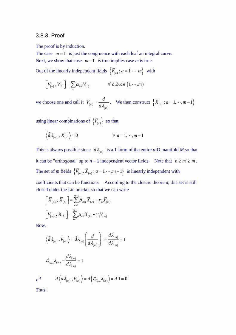
3.8.3. Proof

The proof is by induction.

The case 1m is just the congruence with each leaf an integral curve.

Next, we show that case 1m is true implies case m is true.

Out of the linearly independent fields ; 1, ,aV a m with

, abca b cc

V V V , , 1, ,a b c m

we choose one and call it

mm

dV

d . We then construct ; 1, , 1aX a m

using linear combinations of aV so that

, 0m ad X 1, , 1a m

This is always possible since md is a 1-form of the entire n-D manifold M so that

it can be "orthogonal" up to n – 1 independent vector fields. Note that n m m .

The set of m fields , ; 1, , 1m aV X a m is linearly independent with

coefficients that can be functions. According to the closure theorem, this set is still

closed under the Lie bracket so that we can write

1

1

,m

abc aba b c mc

X X X V

1

1

,m

ab am b b mb

V X X V

Now,

,m m mm

dd V d

d

1m

m

d

d

1

m

m

mVm

d

d

, 1 0mm m mV

d d V d d

Thus:

, , , ,

a a bm a b m b mX Xd X X d X d X

, 0a m bX

d X

where aa

dX

d and

0

a

m

mXa

d

d

since mV and aX are independent.

Similarly,

, , , ,

m m bm m b m b mV Vd V X d X d X

, 0m m bV

d X

Using , 0m ad X , contraction of the closure conditions with md becomes

0 ,ab m md V

0 ,a m md V

Hence:

0ab and 0a

so that

1

1

,m

abca b cc

X X X

1

1

,m

abm b bb

V X X

Thus, ; 1, , 1aX a m alone is closed under the Lie bracket, which means they

form a foliation of the (m–1)-D submanifold. ( Remember that we assumed case

m–1 of the theorem to be true ) By definition, a foliation always has a coordinate

basis. Thus, a linear combination aY of aX exists such that

, 0a bY Y , 1, , 1a b m

Now, if we can construct ; 1, , 1aZ a m from aX such that

1

1

m

aba bb

Z X

, 0m bV Z

, 0a bZ Z , 1, , 1a b m

the proof will be completed. ( ,m aV Z will be the coordinate basis of the m-D

submanifold ).

Starting with , 0m aV Z , we have

0 ,m aV Z m aVZ

1

1m

m

ab bVb

X

1 1

1 1m m

m m

ab abb bV Vb b

X X

1 1

1 1

,m m

ababb m b

b bm

dX V X

d

1 1 1

1 1 1

m m mab

ab bcb cb b cm

dX X

d

1 1

1 1

m mab

ac cb bb cm

dX

d

Since bX are independent, we have

1

1

0m

abac cb

cm

d

d

which is a set of ordinary differential eqs for . ( is fixed for given mV and

aX ). Since a solution for always exists for a given set of initial conditions, the

condition , 0m aV Z can always be satisfied. The initial conditions are chosen

such that aZ are coordinate basis of the (m–1)-D submanifold spanned by aX

so that

, 0a bZ Z

on the submanifold. This is accomplished by setting a aZ Y . Outside the

submanifold, the condition

0 ,mm a aV

V Z Z

means that aZ is the Lie dragging of aY along mV . Since , 0a bY Y we

have , 0a bZ Z because Lie dragging preserves the commutativity of Lie

brackets. QED.

3.9. An Example: The Generators of S2

Consider the (un-normalized) basis vector e of the spherical coordinates , ,r ,

x ye ye xe or y xx y

which we shall called zl , the angular momentum operator along z,

zl

Defining xl and yl analogously, one can prove that [see any quantum mechanics

textbook],

,x y zl l l

,y z xl l l (3.30)

,z x yl l l

Thus, , ,x y zl l l is closed under the Lie bracket so that they form a submanifold of

dimension 3d . In fact, 2d , which can be seen by considering the function

2 2 2r x y z

It can be shown that

0x y zl r l r l r

and

0x y zdr l dr l dr l (3.31)

Since the contraction V is the number of planes of constant that are pierced

by V , eq(3.31) means that , ,x y zl l l are tangent to the 2-D surface r const .

Therefore, 2d and the submanifold is just the 2-D sphere.

To complete the analogy with the angular momentum operator in quantum mechanics,

we define

2

x x y y z zl l l l l lL (3.32)

so that

2, 0jl

L for , ,j x y z

22

2 2

1 1sin

sin sin

f fL f

(3.33)

Proof of these is left as exercise.

3.10. Invariance

A tensor field T is said to be invariant under a vector field V if

0V

T (3.34)

If T is an important characteristic of the system, so is V . For example, an axiallysymmetric system is invariant under rotations in some plane so that the angular

momentum generating them is conserved and characterizes the system.

Theorem

Let 1 2, ,F T T be a set of tensor fields. The set L of all vector fields under

which all fields in F are invariant is a Lie algebra.

Proof

First, we leave as an exercise to show that

0i iV W T T 0iaV bW

T (3.35a)

where a and b are constants. Secondly, using eq(3.8), we have

0i iV W T T ,

, 0i iV W V W T T (3.35)

Thus, if V and W are in L, so are aV bW and ,V W . QED.

Comments

Note that L allows only linear combinations with constant coefficients. Thus, the

corresponding vector space treats each field V as a single element. In contrast, a

fibre bundle allows linear combinations with functions as coefficients so that each

field V is a cross section. For example, the set , ,x y zl l l as considered vectors

in the fibre bundle with base 3 is linearly dependent since they are all tangent to

the spherical surface 2S . However, to express each vector field jl as the linear

combination of the other 2, we must use functions as coefficients. Hence, in the Lie

algebra, the set , ,x y zl l l is linearly independent and form a 3-D basis.

Similarly, the dimension of the Lie algebra of all tangent vector fields to a finite

dimensional manifold is infinite.

3.11. Killing Vector Fields

A Killing vector field V is defined by

0V

g (3.36)

where g is the metric tensor. Given coordinates ix , we have [see eq(3.14)]

0k k kij ik kjk j jV ij

V g g V g Vx x x

g (3.37)

If the integral curves of V are used as the coordinate lines of 1x , eq(3.37) reduces

to [see eq(3.12)]

10ijV ij

gx

g (3.38)

Thus, if a Killing vector is used as a basis vector, the metric will be independent of the

corresponding coordinate. Conversely, if a metric is independent of certain

coordinates, the corresponding basis vectors are Killing vectors.

As an example, consider 3 with Cartesian coordinates , ,x y z so that

ij ijg for , , ,i j x y z (3.39)

Since these are independent of , ,x y z , the basis vectors , ,x y z

are Killing

vectors. In spherical coordinates , ,r , we have

1rrgr r

2g r

(3.40)

2 2sing r

Hence, only zl

is a Killing vector. By symmetry, so are xl and yl . Indeed,

the 6 Killing vectors , , , , ,x y zx y z l l l form a basis for the Lie algebra (of Killing

vector fields). [More in chapter 5]

3.12. Killing Vectors and Conserved Quantities in ParticleDynamics

In classical mechanics, if a particle is subject to an axially symmetric potential, the

component of its angular momentum about the axis of symmetry is a constant on the

particle's trajectory. Similarly, if the potential is independent of the Cartesian

coordinate x, the x-component of the linear momentum is conserved.

However, not every symmetry of the potential can lead to a conserved dynamical

quantity. For example, there is no conserved quantity associated with a potential that

is constant on a family of ellipsoidal surfaces.

The reason for this is that, in order to induce a conserved dynamical quantity, the

symmetry of the potential must be with respect to displacements along some Killing

vector fields of the spacetime manifold. Proof of this will be deferred to §5.8.

In the meantime, consider the equation of motion in ordinary vector calculus

notations,

m V or i imV (3.41)

where is the "gradient" operator. However, as shown in §2.29, is really the

vector gradient so that in non-Cartesian coordinates, eq(3.41) should be written as

i ijj

mV gx

(3.42)

Obviously, any conserved quantities of (3.42) must involve symmetries in both g

and .

3.13. Axial Symmetry

3.13.0. The Problem

3.13.1. Scalar Solutions

3.13.2. Vector Solutions

3.13.0. The Problem

Axial symmetry denotes invariance under arbitrary rotations about a fixed axis. If

there is an additional invariance under arbitrary translations along the axis, the

symmetry becomes cylindrical.

In problems such as particle dynamics, the symmetry is in the "background". For

example, in the motion of a particle subject to a potential with axial symmetry, the

equation of motion is of the form

0L (3.43)

where describes the state of the system. L is some linear operator with axial

symmetry, i.e., it is invariant under transformation const , where is the

angle about the symmetry axis. In other words, L can only depend on partials such

asn

n

but not itself. However, a solution to (3.43) cannot be axially

symmetric since the particle can only be at one place at any given time.

Similar conclusions can also be drawn for the case of adding to an axially symmetric

field a perturbation that has non-axisymmetric initial values.

3.13.1. Scalar Solutions

If is a scalar, one can introduce the Fourier series

, j jm

m

imx x e

(3.44)

so that (3.43) becomes

m mm

im imL L Le e

m mm

im im imL Le e e

0 (a)

Since L is a linear differential operator, we have

jm

im imL f xe e

where fm is some function independent of . Hence, (a) becomes

0 m m mm

imL f e

(b)

Since the terms enclosed in [ ] are independent of , eq(b) can only be satisfied if

0m m m m mim imL f L Le e m

Thus, we can define a -independent operator Lm by

0m m m mim imL L Le e

so that

0m mm

imL Le

Another way to write m mL is

m m m mim im imL L Le e e

mim imLe e (3.45)

Note that the difference between Lm and L is that the former is completely

independent of but the latter can depend on the partials of . For example,

consider the Laplacian operator in ordinary vector calculus written in spherical

coordinates2

2 22 2 2 2 2

1 1 1sin

sin sinr

r r r r r

Obviously, it is invariant under const . Also,

2 , im im imf r f fe e e

2 22im im imf f fe e e

2 2im imf fe e

2

22 2sin

im immf f

re e

22

2 2 2 2

1 1sin

sin sinim m

r fr r r r r

e

(3.46)

Thus, 2L and2

22 2 2 2

1 1sin

sin sinm

mL r

r r r r r

The functions ime are called scalar axial harmonics. A solution of 0L

is said to have axial eigenvalue m if

eim

where ze l

(3.47)

If is a scalar function,

eim

so that is simply proportional to the scalar axial harmonics.

3.13.2. Vector Solutions

Consider the submanifold S defined by 0 with the symmetry axis as a boundary.

Let je be the basis for the tangent space PV of S. It is then supplemented so that

, je e is the basis of the tangent space PT of the manifold M for points in S. A

basis of PT for the entire M can be obtained by Lie dragging , je e along e

once around the symmetry axis. [see Fig.3.8] By definition, the resulting basis

vectors satisfy

0e

e 0je

e

(3.48)

i.e., they are all axially symmetric. Note that the Cartesian coordinate components

of these basis vectors are changed by the Lie dragging. This nicely illustrates the

fact that axial symmetry for a vector field demands - independence of its

components only when is one of the coordinates.

The basis generated by (3.48) has axial eigenvalue 0m . Basis vectors

,m m je e with axial eigenvalue m can be obtained from 0 0, , jje e e e

according to

mime ee and jm j

ime ee (3.49)

so that using (3.48), we have

me e

ime ee

e e

im ime ee e

e

im ee

imim ee mime

jm je e

ime ee

j je e

im ime ee e

je

im ee

jimim ee m jime

as desired. Any vector field with axial eigenvalue m, i.e.,

eV imV

can be expressed as a linear combination of ,m m je e with coefficients that are

functions independent of . In passing, we mention that the Lie draggings along e

form a Lie group called 2SO .

3.14. Abstract Lie Groups

3.14.1. Lie Groups

3.14.2. Lie Algebra

3.14.3. One-Parameter Subgroups

3.14.1. Lie Groups

An n-D Lie group is an n-D C manifold G such that g G , the mappings

:gl G G by gh l h gh [left translation by g]

:gr G G by gh r h hg [right translation by g]

are diffeomorphisms ( C 1-1 onto maps). These induce corresponding mappings

on the tangent spaces:

:g h ghL T T and :g h h gR T T

Of particular interest is the mappings of h in the neighborhood the identity element e.

3.14.2. Lie Algebra

A vector field V on G is left-invariant if Lg maps V at any h to V at gh for all g,

i.e.,

:gL V h V gh ,h g (a)

Note that with the help of the group composition, eq(a) is guaranteed if

:gL V e V g g (b)

Either gL or gR provides a way to compare vectors at different points. For

example, left- or right- invariancy is a natural criterion for a constant vector field V

in M. Now, each eV e T defines a unique left- or right- invariant vector field.

The set of all left- or right- invariant vector fields thus forms a vector space of the

same dimension as eT . [ As in §3.10, the coefficients in the linear combinations of

these fields must be constants, not functions, on G. ] It is easily proved that the Lie

bracket of 2 left(right)- invariant fields is also a left(right)- invariant field. Hence,

the set of all left- or right- invariant vector fields forms a Lie algebra. By convention,

the algebra of the left- invariant fields is called the Lie algebra of G and denoted by

G . Let , 1, ,iV i n be a (left-invariant) basis vector fields for G .

Closure under the Lie bracket means

, kiji j kV V c V (3.50)

The constants kijc are called the structure constants. It can be shown that they are

the components a type1

2

tensor C called the structure tensor. Thus, every Lie

algebra has a unique structure tensor C. The converse of this however not true [see

§3.16]. If 0kijc for all i, j, and k, then G is called abelian. We shall see

that this implies the group G is also abelian.

3.14.3. One-Parameter Subgroups

Consider the integral curve C t of a left-invariant vector field V that passes

through e at 0t . Thus,0

e et

dV V

dt

and other points on C can be obtained

by the exponentiation exp tV [see §2.13]. Alternatively, this can be viewed as

the diffeomorphism of G itself generated by V [see §3.1]. Note that V is left-

invariant so that it is determined entirely by eV . To emphasize this point, we write

expeV e

C t g t tV (3.51)

Now, it is easily proved from the definition of exponentiation that

2 1 2 1exp exp expe e

t V t V t t V

Hence,

1 2 1 2expeV e

g t t t t V 2 1exp expe

t V t V

2 1e eV V

g t g t (3.52)

so that points on C form an abelian group called a one-parameter subgroup of G.Note that each vector in eT generates a unique 1-parameter subgroup denoting a

C curve in G that passes through e. Thus, there is a 1-1 correspondence between

these 1-parameter subgroups and the elements of the Lie algebra.

3.15. Examples of Lie Groups

3.15.1. Rn

3.15.2. GL(n,K)

3.15.3. O(n)

3.15.4. SU(n)

3.15.1. Rn

n is a manifold and an abelian group under vector addition. Hence, it is a Lie

group. The 1-parameter subgroups are the 'rays' (straight lines starting from the

origin), which are also the left- invariant fields. The Lie algebra is abelian.

3.15.2. GL(n,K)

3.15.2.a. Group Manifold

3.15.2.b. 1-Parameter Subgroups

3.15.2.c. Component of the Identity

3.15.2.d. Lie Algebra

3.15.2.a. Group Manifold

Ther general linear group ,GL n in n dimensions is the group of all invertible

nn matrices with elements in or . Group composition is matrix

multiplication with the unit matrix I as identity e. Using the matrix elements as

coordinates, we see that the set of all nn matrices is2n with ,GL n as a

submanifold that excludes all points corresponding to matrices of vanishing

determinants excluded.

Now, the tangent spaces of m are again m . Therefore, the tangent spaces PT

of ,GL n are also submanifolds of2n so that all tangent vectors are also

n n matrices. In fact,2n

PT , i.e., it includes matrices with vanishing

determinants. For example, consider the curve through e given by

1 ,1, ,1P diag e

Thus, det 1 0P e for all so that the curve is in ,GL n . Its tangent

at e is

0

1,0, ,0dP

diagd

0

det 0dP

d

Since2n

PT , any matrix can generate a 1-parameter subgroup and hence belongs

to the Lie algebra ,GL n .

3.15.2.b. 1-Parameter Subgroups

The 1-parameter subgroup generated by a matrix A is the integral curve Ag t of the

left-invariant field V that is equal to A at e. Setting 0t at e, we have

0

A

t

dgA

dt

. Using (3.52), we can write

A A Ag t t g t g t

0limA A A

t

dg t g t t g t

dt t

0lim A A

t

g t g t I

t

Using 0Ag I , we have

0

AA

dgg t I t

dt

so that

0

A AA

dg t dgg t

dt dt Ag t A (3.53)

t AAg t e

0 !

nn

n

tA

n

(3.54,5)

i.e., the 1-parameter subgroups of ,GL n are the exponentiations of arbitrary nn

matrices, which are called infintesimal generators of the subgroup.

3.15.2.c. Component of the Identity

Not every element of ,GL n is a member of a 1-parameter subgroup.

This is because a 1-parameter subgroup Ag t is a continuous curve that passes

through e I with det 1I . Since det Ag is a continuous function of t while

det 0g for all ,g GL n , we have det 0Ag . Therefore, every invertible

real matrix with negative determinant is not on any 1-parameter subgroup. This

means ,GL n is a disconnected group. In general, elements that belong to a

1-parameter subgroups are called the component of the identity of the group.

3.15.2.d. Lie Algebra

Given a tangent vector eA at e anf its 1-parameter subgroup eAg t , the left-

translation eAf g t of this curve by any matrix ,f GL n produces a curve of

the congruence of the left- invariant vector field A generated by eA . If f is on the

curve eB

g t , eq(2.12) gives

20

1, lim

e e e eA B B Ae tA B g t g t g t g t

t

20

1lim exp exp exp expe e e et

tA tB tB tAt

[(3.55) used]

20

1lim e e e et

I tA I tB I tB I tAt

e e e eA B B A (3.60)

which is simply the matrix commutator.

3.15.3. O(n)

3.15.4. SU(n)

3.16. Lie Algebras and Their Groups

3.16.1. General Definition of Lie Brackets

3.16.2. Coverings

3.16.3. SU(2)

3.16.4. Exponentiations for SU(2)

3.16.5. Exponentiations for SO(3)

3.16.6. SU(2) Covers SO(3)

3.16.7. Topologies

3.16.1. General Definition of Lie Brackets

Every Lie group G has its Lie algebra G. Now, every element g G is the image

of e under the left- translation generated by g. Also, every vector e eV T generates

a unique vector field V in G. Therefore, every g is on one curve of each of the

left- invariant congruences. The question is whether it is possible to reconstruct G

given G.

To answer the question, we first generalize the definition of a Lie bracket and hence

that of the Lie algebra. Thus, the Lie bracket is defined as an internal binary

operator on a vector space V on ,

V V V by , ,A B A B

such that for all ,A B V and ,a b ,

1. , ,aA B a A B and , ,A bB b A B . (bilinearity)

2. , ,A B B A . (antisymmetry) (3.68)

3. , , , , , , 0A B C B C A C A B . (Jacobi identity) (3.69)

For example, the cross product of vectors in 3 defines a Lie bracket:

,a b a b 3,a b (3.70)

3.16.2. Coverings

We now state but not prove the following theorems:

1. Every Lie algebra is the Lie algebra of one and only one simply- connected Lie

group.

2. Any Lie group that is multiply- connected can be covered by the simply-

connected one belonging to the same Lie algebra. The covering is then a

homomorphism between these groups.

Note that

1. A manifold is simply- connected if every closed curve in it can be smoothly

shrunk into a point.

2. A connected manifold M covers another manifold N if there is a map

: M N

that is onto and such that for any neighborhood U of a point P N ,

1 1i

i

U U

where 1 U is the inverse image of U and 1i denotes the inverse function

for the ith 1-1 branch of .

For example, the real line covers the unit circle S1 an infinite number of times by

the map

1: S by cos ,sinx x x x

Thus, every interval , 2x x in is mapped onto S1

3.16.3. SU(2)

Consider the set H of matrices of the form

* *

a b

b a

(3.72)

We leave as exercise the proofs of the following:

1. The set0 0

0 0H

is a group under matrix multiplication. It is called the

2,GL .

2. H is a 4-D real vector space under matrix addition. One basis is

1

0102

iJ

i

2

0 111 02

J

3

0102

iJ

i

1 0

0 1I

3. Writing A H as

1 1 2 2 3 3 42 2 2A J J J I

where j are real. We have ASU(2) iff

4

1

1jj

(3.73)

4. There is a 1-1 onto mapping from SU(2) to the spherical surface 3S .

Since 3S is simply- connected, so is SU(2).

3.16.4. Exponentiations for SU(2)

Elements of SU(2) can be obtained by the exponentiation of the elements of [SU(2)].

For example, using

1

0 1

1 02

iJ

2 221

1 0

0 12 2

i iJ I

3 231 1

0 1

1 02 2

i iJ J

so that

2 1 21 1 1

nnJ J J 2

12

ni

J

2 21 1

nnJ J2

2

ni

I

0,1,n

the exponentiation of J1 gives

2 2 1

2 2 11 1 1

0 0

exp2 ! 2 1 !

n nn n

n n

t ttJ J J

n n

2 12 2

10 0

12

2 ! 2 2 1 ! 2

nn n

n n

it i tI J

n n

1cos 2 sin2 2

t tI J

cos sin2 2

sin cos2 2

t ti

t ti

(3.74)

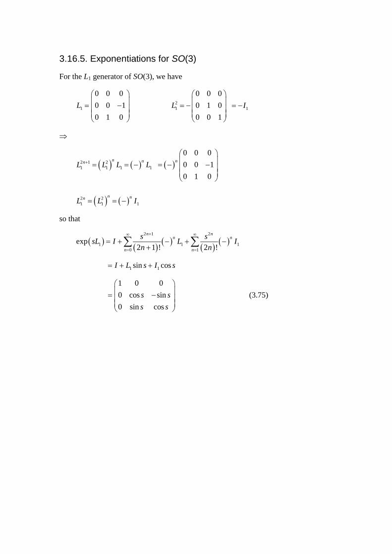
3.16.5. Exponentiations for SO(3)

For the L1 generator of SO(3), we have

1

0 0 0

0 0 1

0 1 0

L

21

0 0 0

0 1 0

0 0 1

L

1I

2 1 21 1 1 1

n nnL L L L 0 0 0

0 0 1

0 1 0

n

2 21 1 1

n nnL L I

so that

2 1 2

1 1 10 1

exp2 1 ! 2 !

n nn n

n n

s ssL I L I

n n

1 1sin cosI L s I s

1 0 0

0 cos sin

0 sin cos

s s

s s

(3.75)

3.16.6. SU(2) Covers SO(3)

The exponentiations given by (3.74-5) suggests a mapping

: 2 3SU SO

by

1 1exp exptJ tL

i.e.,

1 0 0cos sin2 2 0 cos sin

sin cos 0 sin cos2 2

t ti

t tt t

i t t

(3.76)

Now, the distinct elements in 1exp tL are represented by any interval

, 2t a a of length 2 and those in 1exp tJ by , 4t a a of length 4.

Thus, 1exp tJ doubly covers 1exp tL . Similar conclusions can be drawn for

the other generators so that the map

: 2 3SU SO

by

3 3

1 1

exp expj j j jj j

t J t L

(3.77)

is a double covering of SO(3) by SU(2).

3.16.7. Topologies

As mentioned in §3.16.3, the manifold SU(2) is diffeomorphic to the simply

connected S3 and hence share the same global topology. A one-parameter subgroup

1exp tJ of SU(2) begins at e with 0t and returns to it at 4t , thus tracing

out a great circle on S3. The points labelled t and 2t are diametrically opposite

to each other. Since they are mapped to the same point in SO(3), we see that SO(3)

is a hemisphere of S3. The manifold SO(3) is not simply connected because the great

circle forming its boundary cannot be shrunk since points on it must be pairwise

diametrically opposite. Note that locally, SU(2) and SO(3) are identical so that they

have the same Lie algebra.

The Lie algebra using the cross product as Lie bracket [see (3.70)] can be associated

with either group SU(2) or SO(3). In classical mechanics, cross products in 3 are

usually associated with SO(3) so that elements of the subgroup exp jL

correspond to rotations about the xj axis. However, this identification of rotations

with vectors works only in 3 . For example, vectors in 4 are 4-D but the

rotation group SO(4) is 6-D so that no such identification is possible. In quantum

mechanics, associating SU(2) with 3 allows the assignment of the spin to a vector

in 3 even though the spin is not an element of the tangent space of 3 .

Finally, we mention that the algebra of an abelian group must be abelian.

3.17. Realizations and Representations

3.17.1. Definitions

3.17.2. Example 1

3.17.3. Example 2

3.17.4. Example 3

3.17.1. Definitions

Mathematically, a group, say SO(3), is an abstract group defined entirely by its

group operation and manifold topology. However, in applications in physics, the

importance of a group is its action on physical quantities. For example, elements of

SO(3) are associated with rotations of objects in 3-D space. Such an association is

called a realization. Let T M be the set of operators on some space M . A

realization of a group G is a map

:T G T M by g T g

such that the group properties are preserved, i.e.,

1. T e I where I is the identity transformation on M.

2. 11T g T g .

3. T g T h T gh where is the composition in T M .

A realization is faithful if T is 1-1, i.e.,

g h T g T h

If M is a vector space and T(g) are linear transformations, the realization is called a

representation.

3.17.2. Example 1

Consider the unit sphere 2S in 3 given by 2 2 2 1x y z . A rotation by

about the x-axis maps a point , ,x y z to another , ,x y z according to

x x cos siny y z (3.78)

sin cosz y z

so that2 2 2 1x y z

This transformation can be associated with an element in the subgroup 1exp L of

SO(3) . If we treat it as a transformation of 2S into itself, we have a realization of

SO(3) since 2S is not a vector space. On the other hand, if we treat it as

transformations in 3 , which is a vector space, we have a representation of SO(3).

The fact that, originally, we have used rotations in 3 to define SO(3) illustrates a

useful technique. Thus, a group is first defined by a faithful realization or

representation so that its properties can be studied in concrete terms. Afterwards, the

group is regarded as abstract to allow for other useful realizations and representations.

3.17.3. Example 2

Every group G has at least 2 faithful realizations: the left and right translations of

itself. The left translations give rise to the progressive (principal) realization and

the right translations to the retrograde realization.

3.17.4. Example 3

Each Lie group G has a representation using its elements as linear transformations on

its own Lie algebra. This is called the adjoint representation and is defined as

follows. First, we define the adjoint realization of the group G by the mappings

:gI G G by 1gh I h ghg ,g h G

which is not necessarily faithful. For example, if G is abelian, Ig is the identity map

h h for all g. The mappings Ig are inner automorphisms of G. Note that

1gI e geg e for all g so that every curve through e is mapped to another curve

through e. Thus, Ig induces another map

:g e eAd T T

called the adjoint transformation of Te induced by g. Given a 1-parameter

subgroup exp t X where eX T , its image under Ig is another 1-parameter

subgroup with composition

1 1 1gfg ghg g fhg

This defines the action of Adg as

exp expg gI t X t Ad X (3.79)

If g is also a member of the 1-parameter subgroup expg s sY , it is left as an

exercise to show that

expg s YAd X s X (3.80)

3.18. Spherical Symmetry, Spherical Harmonics andRepresentations of the Rotation Group

3.18.1. Preliminary

3.18.2. Spherical Symmetry

3.18.3. SO(3) and SU(2)

3.18.1. Preliminary

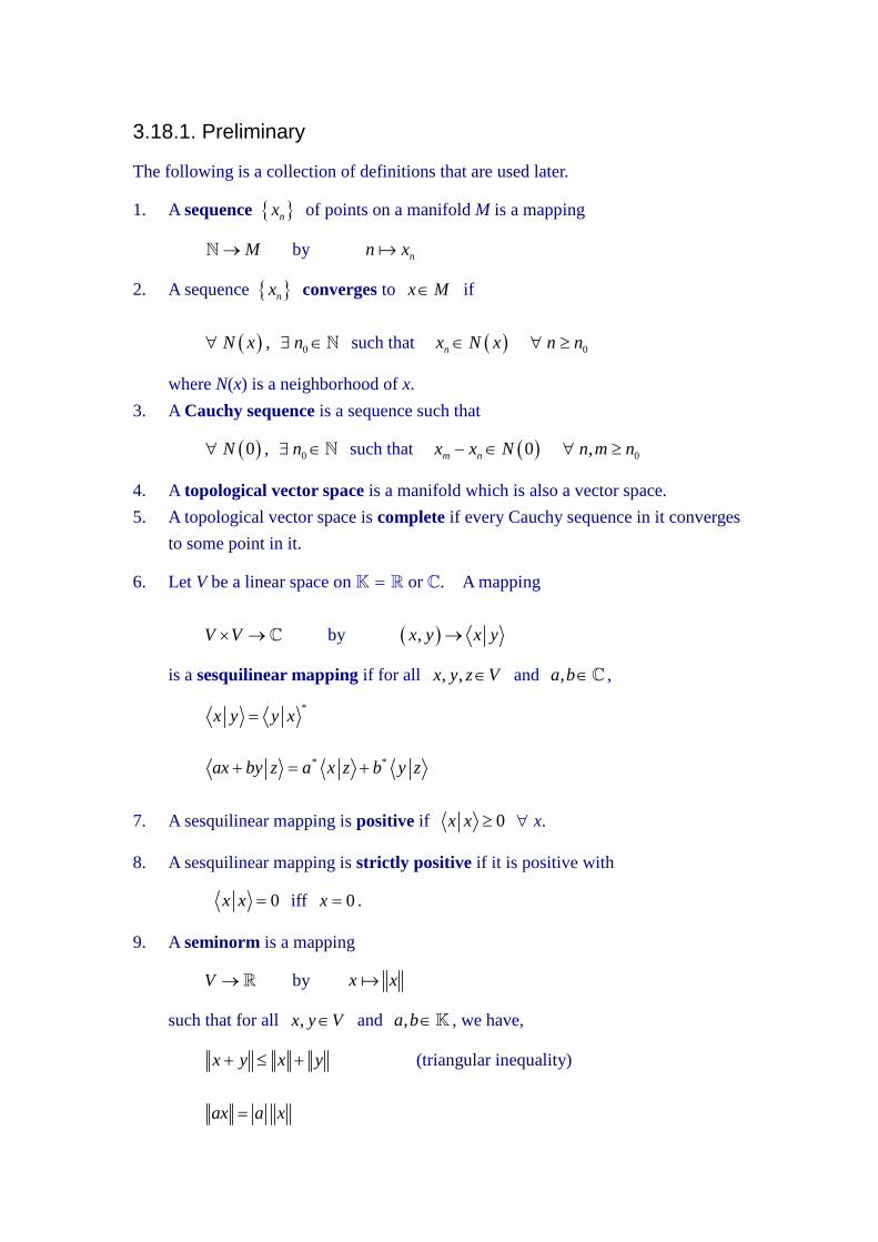
The following is a collection of definitions that are used later.

1. A sequence nx of points on a manifold M is a mapping

M by nn x

2. A sequence nx converges to x M if

N x , 0n such that nx N x 0n n

where N(x) is a neighborhood of x.

3. A Cauchy sequence is a sequence such that

0N , 0n such that 0m nx x N 0,n m n

4. A topological vector space is a manifold which is also a vector space.

5. A topological vector space is complete if every Cauchy sequence in it converges

to some point in it.

6. Let V be a linear space on or . A mapping

V V by ,x y x y

is a sesquilinear mapping if for all , ,x y z V and ,a b ,

*x y y x

* *ax by z a x z b y z

7. A sesquilinear mapping is positive if 0x x x.

8. A sesquilinear mapping is strictly positive if it is positive with

0x x iff 0x .

9. A seminorm is a mapping

V by x x

such that for all ,x y V and ,a b , we have,

x y x y (triangular inequality)

ax a x

If furthermore,

0x iff 0x

it is a norm.

10. A complete normed vector space is called a Banach space.

11. A linear space with a strictly positive sesquilinear mapping is called a

pre–Hilbert space & the mapping the inner product.

12. The inner product induces a norm x x x .

13. A complete pre-Hilbert space is called a Hilbert space.

14. The space of all functions f on M such thatp

f is integrable is called pL M .

3.18.2. Spherical Symmetry

A manifold M is spherically symmetric if the Lie algebra of its Killing vector fields

has a subalgebra 3 3so SO . Consider the Hilbert space H(S2) on S2 which

is the linear ( function ) space L2(S2) of all square- integrable complex functions on S2.

A vector in L2(S2) is a function f with norm

2

*

S

f dx f x f x where f(x) is the component of the vector f in the basis consists of eigenfunctions of

the position operator. Note that L2(S2) is a vector space of infinite dimensions.

The realization of 3g SO as a mapping

2 2:R g S S by x x R g x

induces a mapping

2 2 2 2:g L S L S by f f g f

With suitable definitions, g can be made to be a representation of SO(3) on

L2(S2). Since L2(S2) is infinite dimensional, so is g .

There are also finite dimensional subspaces of L2(S2) that are invariant under g

g. They form representations of finite dimensions. Invariant subspaces that

contain no smaller invariant subspaces give irreducible representations (IRs).

Let ; 1, ,if i N be a basis for such an invariant subspace 2 2V L S , then

iif a f f V

iig f g a f i

ia g f f iib f

which implies

ji j ig f f g

such that

i j i jj i i ja f g b f b f j j i

ib g a

The matrix ii j jm g is called the representation of g in V.

The basis functions of finite dimensional IRs for SO(3) are the spherical harmonics lmY .

( see Tung for the actual construction ).

Thus, each invariant subspaces Vl of L2(S2) is characterized by an integer 0l and

has dimension 2 1l . The set ; , ,l lmY Y m l l is a basis of Vl. The

spherical harmonics are complete in the sense that

0l

l

Y Y

; 0,1, ; , ,lmY l m l l

is a basis for L2(S2).

Since exp iiR g t l and exp i

ig t , Vl is invariant under g iff it is

invariant under ; , ,i i x y z . This is guaranteed if the basis Yl is invariant under

the generators ; , ,i i x y z , i.e.,

ii lm lmY Y k l k

k

c Y , ,i x y z and , ,m l l

For example, if 0l ,

0 00 1Y Y

00 00i

i Y Y 001 0 0i Y , ,i x y z

For 1l ,

1 11 10 1 1, ,Y Y Y Y 3 3 3

sin , cos , sin8 4 8

i ie e

3 3 3, ,

8 4 8x iy z x iy

Thus

1

3

8x ll Y y z x iyz y

3

8zi

10

2

iY

1

3

8z ll Y x y x iyy x

3

8ix y

3

8i x iy

1 1i Y

1l is the smallest faithful representation of SO(3). It is usually called the

fundamental representation. Obviously, it is equivalent to the defining 33 special

orthogonal matrix representation. ( see Ex 3.26, Schultz )

3.18.3. SO(3) and SU(2)

Since : 2 3SU SO is a 2-1 mapping, i.e., there are 2 elements u, u' SU(2)

that maps into the same g SO(3), therefore, any representation R(g) of g SO(3)

defines a ( unfaithful ) representation S for SU(2) such that

S u S u R u R u

Other representations, say T , of SU(2) such that

T u T u even if u u

are called double valued representations of SO(3).

IRs of SU(2) are characterized by an index k which is either a whole or a half integer.

If k is an integer, they are representations of SO(3) with the same index ( l k ).

If k is a half- integer, they're double- valued representations of SO(3).

The 22 special unitary matrices used to define SU(2) form a representation with

1

2k . It is the smallest faithful representation & often called the spin

1

2

representation. Elements of the vector space are called spinors.

3.19. Bibliography