liangyuan hu1,2,3, chenyang gu4, michael lopez5, jiayi ji

Estimation of Causal Effects of MultipleTreatments in Observational Studieswith a Binary Outcome

Journal TitleXX(X):1–15c©The Author(s) 2016

Reprints and permission:sagepub.co.uk/journalsPermissions.navDOI: 10.1177/ToBeAssignedwww.sagepub.com/

SAGE

Liangyuan Hu1,2,3, Chenyang Gu4, Michael Lopez5, Jiayi Ji 1,2,3, Juan Wisnivesky 6

AbstractThere is a dearth of robust methods to estimate the causal effects of multiple treatments when the outcome is binary.This paper uses two unique sets of simulations to propose and evaluate the use of Bayesian Additive RegressionTrees (BART) in such settings. First, we compare BART to several approaches that have been proposed for continuousoutcomes, including inverse probability of treatment weighting (IPTW), targeted maximum likelihood estimator (TMLE),vector matching and regression adjustment. Results suggest that under conditions of non-linearity and non-additivityof both the treatment assignment and outcome generating mechanisms, BART, TMLE and IPTW using generalizedboosted models (GBM) provide better bias reduction and smaller root mean squared error. BART and TMLE providemore consistent 95 per cent CI coverage and better large-sample convergence property. Second, we supply BART witha strategy to identify a common support region for retaining inferential units and for avoiding extrapolating over areasof the covariate space where common support does not exist. BART retains more inferential units than the generalizedpropensity score based strategy, and shows lower bias, compared to TMLE or GBM, in a variety of scenarios differingby the degree of covariate overlap. A case study examining the effects of three surgical approaches for non-small celllung cancer demonstrates the methods.

KeywordsCausal inference; Generalized propensity score; Inverse probability of treatment weighting; Matching; Machine learning

Introduction

Motivating Research QuestionLung cancer is the leading cause of cancer-related mortality worldwide and is estimated to have caused over 1.7 milliondeaths in 20181. The most common type of lung cancer is non-small cell lung cancer (NSCLC), accounting for approximately85% of all lung cancer cases2. When feasible, NSCLC tumors are treated using surgical resection, which remains the mosteffective option for a cure3.

Open thoracotomy long stood as the standard surgical procedure for stage I-IIIA NSCLC tumors. However, openthoracotomy is associated with considerable postoperative complications and mortality, especially in the elderly4,5.Beginning in the late 1990s, two newer and less invasive techniques, video-assisted thoratic surgery (VATS) and, morerecently, robotic-assisted surgery, were increasingly used6,7. The adoption of VATS and robotic-assisted surgery seemedto signal that the newer procedures offer a clinical benefit relative to open resection8,9. However, to our knowledge, norandomized controlled trials (RCTs) have been conducted to compare the effectiveness of these surgical procedures, in partdue to difficulties in recruiting patients and high study costs. As a consequence, VATS and robotic-approaches were adoptedinto routine care without sufficient scrutiny6,10.

In place of RCTs, large-scale population-based databases, such as the Surveillance, Epidemiology, and End Results(SEER)-Medicare database, provide research opportunities for comparative studies. The SEER-Medicare database comprises

1Department of Population Health Science and Policy, Icahn School of Medicine, New York, USA2Institute for Health Care Delivery Science, Icahn School of Medicine, New York, USA3Tisch Cancer Institute, Icahn School of Medicine, New York, USA4Analysis Group, Inc., Los Angeles, USA5National Football League, New York, NY6Department of Medicine,Icahn School of Medicine, New York, NY

Corresponding author:Liangyuan Hu, Center for Biostatistics, Department of Population Health Science and Policy, Ichan School of Medicine, New York, NY, 10029, USA.Email: [email protected]

Prepared using sagej.cls [Version: 2017/01/17 v1.20]

arX

iv:2

001.

0648

3v1

[st

at.M

E]

17

Jan

2020

2 Journal Title XX(X)

a large sample of patients who received each of the three surgical procedures and reflects patient outcomes in the real worldsetting, containing demographic and clinical information for Medicare beneficiaries with cancer in various United Statesregions11. However, in contrast to RCTs, the real-world adoption pattern of the three surgical approaches largely dependson the patients’ sociodemographic and tumor characteristics, which may result in an unbalanced cohort with significantdifferences in the distributions of sociodemographic characteristics, comorbidities, cancer characteristics and diagnosticinformation across treatment groups12.

The research question poses several challenges for statistical analyses. First, in practice, statistical methods designedfor a binary treatment are often used to account for underlying differences in patient characteristics to compare each pairof surgical procedures6,10,13. Unfortunately, applications of these methods can lead to the comparisons of disparate patientsubgroups, which may increase bias in treatment effect estimates14. Second, common measures for comparative effectivenessare postoperative complications, which are binary outcomes. Thus, the treatment effects are typically based on the riskdifference (RD), odds ratio (OD) or relative risk (RR)15, all of which make it less straightforward to obtain inference,relative to continuous outcomes16–18. Third, the robotic-assisted surgery is a new advanced technology that was just adoptedinto practice in recent years. As a result, the number of patients who are operated via this approach is smaller compared tothe other two approaches, yielding unequal sample sizes across the treatment groups. Appropriate causal inference methodsthat can address these challenges are needed.

Overview of Methods for Causal Inference with Multiple TreatmentsRecent years have seen a growing interest in the development of causal inference methods with multiple treatments usingobservational data. The theoretical work of Imbens19 and Imai and Van20 extended the propensity score framework in thesetting with a binary treatment21 to the general treatment setting. Subsequently, methods designed for a binary treatmenthave been reformulated to accommodate multiple treatments, including regression adjustment (RA)22, inverse probabilityof treatment weighting (IPTW)23,24, and vector matching (VM)14. Lopez and Gutman14 provide a comprehensive review ofcurrent methods for multiple treatments. These methods focus on continous outcomes.

RA22,25,26, also known as model-based imputation27 uses a regression model to impute missing outcomes, estimating whatwould have happened to a specific unit had this unit received the treatment to which it was not exposed. The causal estimandof interest can be estimated by contrasting the imputed potential outcomes between treatment groups. The critical part ofthis method is the specification of the functional form of the regression model. With a low-dimensional set of pre-treatmentcovariates, it is relatively easy to specify a flexible functional form for the regression model. If there are many pre-treatmentcovariates, however, such a specification is more difficult, and possible misspecification of the regression model could biasthe estimate of treatment effects. RA also heavily relies on extrapolation for estimation when the covariate distributionsbetween treatment groups are far apart27.

IPTW19,23,24 methods attempt to obtain an unbiased estimator for treatment effects in a way akin to how weighting bythe inverse of the selection probability adjusts for unbalances in sampling pools, introduced by Horvitz and Thompson28

in survey research. A challenge with IPTW is that treated units with low generalized propensity scores that are close tozero can result in extreme weights, which may yield erratic causal estimates with large sample variances29,30. This issue isincreasingly likely as the number of treatments increases14. An alternative method is to use trimmed or truncated weights, inwhich weights that exceed a specified threshold are each set to that threshold31,32. The threshold is often based on quantilesof the distribution of the weights (e.g., the 1st and 99th percentiles).

Alternatives to estimate generalized propensity scores in the IPTW framework include generalized boosted models24

(GBM) and Super Learner33,34 (SL). GBM grows multiple regression trees to capture complex and nonlinear relationshipsbetween treatment assignment and pre-treatment variables. The estimation procedure can be tuned to find the generalizedpropensity score model producing the best covariate balance between treatment groups. This feature of GBM should helpalleviate extreme weights and improve the estimation of causal effects24. However, the algorithm can be computationallyintensive, and the robust procedure for estimating the variances of the effect estimates is not guaranteed to result inproper confidence intervals. SL uses ensemble of machine learning approaches including regression, ridge regression, andclassification trees, to estimate a weight for each treatment. There is no guarantee that these probabilities sum to 1, and it iscommon to normalize weights accordingly. To limit extreme weights, Rose and Normand34 use a lower bound of 0.025 foreach probability.

Targeted Maximum Likelihood Estimation34,35 (TMLE) is a doubly robust approach that combines outcome estimation,IPTW estimation, and a targeting step to optimize the parameter of interest with respect to bias/variance. Rose andNormand34 implements TMLE by estimating both generalized propensity scores and a binary outcome using SL. Forobtaining variance estimates, Rose and Normand34 uses influence curves, though bootstrapping is also suggested. The useof TMLE has, to the best of our knowledge, not been deeply vetted for multiple treatment options by using simulations.

Lopez and Gutman14 proposed the VM algorithm, which can match units with similar vector of generalized propensityscores. VM is designed to replicate a multi-arm randomized trial by generating sets of units that are roughly equivalenton measured pre-treatment covariates. VM obtains matched sets using a combination of k-means clustering and one-to-one matching with replacement within each cluster strata. Simulations demonstrated that, relative to IPTW with thegeneralized propensity scores estimated using multinomial logistic regression, and to generalizations of tools designed forbinary treatment, VM yielded lower bias in the covariates’ distributions between different treatment groups, while retaining

Prepared using sagej.cls

Hu et al. 3

most of eligible units that received the reference treatment14. However, the authors acknowledge that there is a lack ofguidance regarding the estimation of the sampling variance, and this is an area for further statistical research.

Before describing BART – one tool that we think is equipped to handle the complexity of causal inference with multipletreatments – it is worth explicating on why one approach that, although intuitive and easy to perform, is not recommended: aseries of binary comparisons (SBC). To wit, grouping subjects into separate sub-populations, each with two treatments, andthen using approaches designed for binary treatment is an approach often used in practice14. However, SBC can (i) lead tonon-transitive causal estimates, (ii) increase bias, and (iii) leave it unclear which treatment is optimal, all of which make itinappropriate for causal inference when there are more than two treatments14.

Bayesian Additive Regression Trees for Causal InferenceWhile the advanced regression and propensity score-based techniques described above were created for causal inference withmultiple treatments, these methods were developed with continuous outcomes in mind, and they have been less studied inthe context of both a binary outcome and multiple treatments.

In recent years, Bayesian Additive Regression Trees (BART)36,37, a nonparametric modeling tool, has become morepopular in causal settings. Hill38 proposed the use of BART for causal inference with a binary treatment and a continuousoutcome. Hill38 and Hill and Su39 used simulations to show that, in scenarios where there are nonlinearities in the responsesurface and the treatment assignment mechanism, BART generates more accurate estimates of average treatment effectscompared to various matching and weighting techniques, and comparable estimates in linear settings.

BART boasts several advantages for causal inference with a binary treatment38,40. First, BART allows for an extremelyflexible functional form. Second, BART avoids ambiguity with respect to covariate balance diagnostics required bypropensity score based approaches. Third, BART generates coherent uncertainty intervals for treatment effect estimates fromthe posterior samples in contrast to propensity score matching and subclassification, for which there is lack of agreementregarding appropriate interval estimation20,38. Finally, BART is easy to implement and requires less researcher programmingexpertise. However, like any methods that do not first discard units that fall out of areas of the covariate space where commonsupport does not exist, one vulnerability of BART is that there is no mechanism to prevent it from extrapolating over theseareas.

We surmise that the strengths of BART are transferable to the multiple treatment setting. In the sections that follow,we conduct two sets of simulations to investigate the operating characteristics of BART for estimating the causal effectsof multiple treatments on a binary outcome, and compare BART to the existing methods discussed previously. We furthersupply BART with a strategy to identify a common support region and compare it to the propensity score based strategy withrespect to the proportion of units retained for inference and the accuracy of treatment effect estimates based on the retainedinferential units. We subsequently apply the methods examined to analyze a large data set on stage I-IIIA NSCLC patients,drawn from the SEER-Medicare registry, and estimate the comparative effect of robotic-assisted surgery versus VATS andopen thoracotomy on postoperative outcomes.

Potential Outcomes Framework for Multiple Treatments

Notation and AssumptionsOur notation is based on the potential outcomes framework, which was originally proposed by Neyman41 in the context ofrandomization-based inference in experiments. Potential outcomes were generalized to observational studies and Bayesiananalysis by Rubin42–44, in what is now known as the Rubin Causal Model (RCM)45.

Consider a sample of N units, indexed by i = 1, . . . , N , drawn randomly from a target population, which comprisesindividuals in a study designed to evaluate the effect of a treatment W on some outcome Y . Each unit is exposed to one oftotal Z possible treatments; that is, Wi = w if individual i was observed under treatment w, where w ∈ W = {1, 2, . . . , Z}.The number of units receiving treatment w is nw, where

∑Zw=1 nw = N . For each unit i, there is a vector of pre-treatment

covariates, Xi, that are not affected by Wi. Let Yi be the observed outcome of the ith unit given the assigned treatment,and {Yi(1), . . . , Yi(Z)} the potential outcomes for the ith unit under each treatment of W . For each unit, at most oneof the potential outcomes is observed (the one corresponding to the treatment to which the unit is exposed). All otherpotential outcomes are missing, which is known as the fundamental problem of causal inference45. Let r(w,Xi) bethe generalized propensity score (GPS), which is defined as the probability of receiving treatment w given pre-treatmentcovariates, that is, r(w,Xi) = Pr(Wi = w|Xi), for ∀ w ∈ {1, . . . , Z}19,20. This definition extends the propensity score21

from a binary treatment setting to the multiple treatment setting, in which conditioning must be done on a vector of GPSs,defined as R(Xi) = (r(1,Xi), . . . , r(Z,Xi)), or a function of R(Xi)

20. In addition, we define the response surface asf(w,Xi) ≡ E[Yi(w)|Xi], for w ∈ {1, . . . , Z}.

In general, causal effects are not identifiable without further assumptions because only one of the potential outcomes isobserved for every unit. We make the following identifying assumptions:

1. The stable unit treatment value assumption (SUTVA)46, that is, no interference between units and no different versionsof a treatment.



2. The positivity or sufficient overlap assumption; that is, 0 < p(Wi|Yi(1), . . . , Yi(Z),Xi) < 1, ∀Wi ∈ {1, . . . , Z},which implies that there are no values of pre-treatment covariates that could occur only among units receiving one ofthe treatments.

3. The treatment assignment is unconfounded; that is, p(Wi|Yi(1), . . . , Yi(Z),Xi) = p(Wi|Xi), ∀Wi ∈ {1, . . . , Z},which implies that the set of observed pre-treatment covariates, Xi, is sufficiently rich such that it includes all variablesdirectly influencing both Wi and Yi; in other words, there is no unmeasured confounding.

Under the unconfoundedness assumption, for any treatment w and pre-treatment covariates Xi,

f(w,Xi) = E[Yi(w)|Wi = w,Xi] = E[Yi|Wi = w,Xi], (1)

where the second identity is the conditional mean function of the observed outcomes.

Definition of Causal EffectsCausal effects are summarized by estimands, which are functions of the unit-level potential outcomes on a common set ofunits42,44. For dichotomous outcomes, causal estimands can be the RD, OD or RR. For purposes of illustration, we use RDin this paper.

Following Lopez and Gutman14, we provide a broad definition of the causal risk difference that may be of interest withmultiple treatments. Define s1 and s2 as two subgroups of treatments such that s1, s2 ⊂ W and s1 ∩ s2 = ∅. Next, let |s1|and |s2| be the cardinality of s1 and s2, respectively. Two commonly used causal estimands are the average treatment effect(ATE), ATEs1,s2 , and the average treatment effect among those receiving s1, ATTs1|s1,s2 , where

ATEs1,s2 = E

[∑w∈s1 Yi(w)

|s1|−∑

w′∈s2 Yi(w′)

|s2|

],

ATTs1|s1,s2 = E

[∑w∈s1 Yi(w)

|s1|−∑

w′∈s2 Yi(w′)

|s2|

∣∣∣∣Wi ∈ s1].

(2)

In (2), the expectation is over all units, i = 1, . . . , N , and the summation is over the potential outcomes of a specific unit.Another set of causal estimands are the conditional treatment effects, given pre-treatment covariates Xi,

CATEs1,s2 = E

[∑w∈s1 Yi(w)

|s1|−∑

w′∈s2 Yi(w′)

|s2|

∣∣∣∣Xi; θY |X

]CATTs1|s1,s2 = E

[∑w∈s1 Yi(w)

|s1|−∑

w′∈s2 Yi(w′)

|s2|

∣∣∣∣Wi ∈ s1,Xi; θY |X

] (3)

where the parameters θY |X and θX index the conditional distribution p(Y |X) and distribution p(X), respectively.Causal inference methods via modeling the response surfaces (e.g., BART and RA) arrive at the population or sample

marginal treatment effects by integrating the conditional effects over the distribution of Xi47. In most cases, however, it is

difficult to model the possibly multi-dimensional Xi. We can obtain the marginal effects by averaging the treatment effectsconditional on the observed values of the covariates over the empirical distribution of {Xi}Ni=1,

ATEs1,s2 =

∫CATEs1,s2(X, θY |X)dFX(X; θX)

ATTs1|s1,s2 =

∫CATTs1|s1,s2(X, θY |X)dFX(X; θX),

(4)

In our motivating example, one of the research questions of interest is to compare the effectiveness of a newer minimally-invasive procedure (i.e., robotic-assisted surgery) versus the existing surgical procedures (e.g., VATS) in the overallpopulation, or among those patients who received robotic-assisted surgery. The corresponding target causal estimands aredefined as

ATE1,2 =

∫E[Yi(1)− Yi(2)|Xi; θY |X ]dFX(X; θX)

ATT1|1,2 =

∫E[Yi(1)− Yi(2)|Wi = 1,Xi; θY |X ]dFX(X; θX).

(5)

Treatment effects using BARTUnder the identifying assumptions, treatment effects such as ATT1|1,2 can be estimated by contrasting the imputed potentialoutcomes between robotic-assisted surgery and VATS groups among those patients who received robotic-assisted surgery,predicted from the estimates of the respective response surface models. In principle, any method that can flexibly estimatef(w,Xi) could be used to predict the potential outcomes.36,37 demonstrated that BART has important advantages as a


Hu et al. 5

predictive algorithm over alternative methods in the machine learning literature such as classification and regression trees48,boosting49 and random forests50, in particular with regard to choosing tuning parameters and generating coherent uncertaintyintervals.

BART is a Bayesian ensemble method that models the mean outcome given predictors by a sum of trees. For a binaryoutcome, the BART model can be expressed using the probit model setup as:

f(w,Xi) = E(Yi|Wi = w,Xi) = Φ

{ J∑j=1

gj(w,Xi;Tj ,Mj)

}, (6)

where Φ is the the standard normal c.d.f., each (Tj ,Mj) denotes a single subtree model in which Tj denotes the regressiontree and Mj is a set of parameter values associated with the terminal nodes of the jth regression tree, gj(w,Xi) representsthe mean assigned to the node in the jth regression tree associated with covariate value Xi and treatment level w, and thenumber of regression trees J is considered to be fixed and known. The details of the specification of prior distribution andthe choice of hyper-parameters can be found in Chipman et al.37. Sampling from the posterior distributions proceed via aBayesian backfitting MCMC algorithm37. A total of L Markov Chain Monte Carlo (MCMC) samples of model parameters,(Tj ,Mj), are drawn from their posterior distribution. For each of L draws, we predict the potential outcomes for eachunit and the relevant treatment level. The causal estimand of interest can be estimated by contrasting the imputed potentialoutcomes between treatment groups. For example, ATT1|1,2 can be estimated as follows:

ATT 1|1,2 = (n1L)−1L∑

l=1

∑i:Wi=1

{f l(1,Xi)− f l(2,Xi)

}

= (n1L)−1L∑

l=1

∑i:Wi=1

{Φ

[ J∑j=1

gj(1,Xi;Tlj ,M

lj)

]− Φ

[ J∑j=1

gj(2,Xi;Tlj ,M

lj)

]},

(7)

where (T lj ,M

lj) are the lth draw from the posterior distribution of (Tj ,Mj). We can obtain obtain the point and interval

estimates of the treatment effect directly using the summary of posterior samples.

Common SupportBecause problems can arise when drawing inference to regions of the covariate space where there are insufficient number ofunits in all treatment groups, propensity score based methods are typically equipped with strategies for defining a commonsupport region. For BART, there is no such a mechanism to prevent it from extrapolating over areas where a common supportdoes not exist.

For a binary treatment, one strategy is to discard units that fall beyond the range of the propensity score51,52. Hill andSu39 argue that these strategies typically ignore the information embedded in the response variable, and propose alternativediscarding rules. Illustrative examples with one or two predictors were used to compare the two types of discarding strategiesand their implications on estimation of the causal effects and the proportion of inferential units retained. Advantages ofBART over the propensity score approach manifest in examples where there is lack of common support for variables onlypredictive of treatment but not of the outcome or the treatment mechanism is more difficult to model. However, in practice,identifying common support is often required for a high-dimensional covariate space. In addition, the two types of strategieshave not been compared in the multiple treatment setting.

To address these limitations, we propose a strategy for BART to define both a common support region and thecorresponding discarding rules. Whereas Hill and Su39 uses a common support for binary treatment using the 1 sd rule,our empirical simulations suggest this rule may be too relaxed in the setting of three or more treatment groups. We use asharper cutoff and identify a common support as follows. We discard any unit i, with Wi = w, for which sfw′

i > maxj{sfwj }, ∀j : Wj = w, where sfwj and sfw′

j denote the standard deviation of the posterior distribution of the potential outcomes undertreatment W = w and W = w′, respectively, for a given unit j.

For multiple treatments with Z = 3, when estimating the ATT of treatment W = 2 and W = 3 among those treated withW = 1, we discard for unit i with Wi = 1, if

sf2i > maxj{sf1j }, and

sf3i > maxj{sf1j }.(8)

When estimating the ATE, we apply the discarding rule in (8) to each treatment group.There is likewise a lack of consensus for defining a common support region with GPS-based approaches. For matching

using the GPS,14 propose a rectangular support region. Let r(w,X) denote the treatment assignment probability for w, andlet r(w,X|W = w′) represent treatment assignment probability forw among those who received treatmentw′. A rectangularcommon support region can be defined as follows with Z = 3. For any w,w′ ∈ W = {1, 2, 3},

r(w,X)low = max{min(r(w,X|W = 1)),min(r(w,X|W = 2)),min(r(w,X|W = 3))}r(w,X)high = min{max(r(w,X|W = 1)),max(r(w,X|W = 2)),max(r(w,X|W = 3))}

(9)



For weighting methods, techniques such as trimming32 or stabilizing (more useful for time-varying confounding, see Huet al.53, Hu and Hogan54 and Hernan and Robins55) are frequently used in place of a common support. However, the lack ofcommon support in the covariate space may lead to extreme weights and unstable IPTW estimators.

Simulation Studies

Design and implementationWe conduct expansive simulations in order to better understand how BART will work in complex causal settings. Our firstset of simulations, Simulation 1, contrasts BART with other approaches, while our second set, Simulation 2, looks into therole that covariate overlap plays in inferences with multiple treatments.

The design of both simulations mimics the range of scenarios that are representative of the data structure in the SEER-Medicare registry. Three treatment levels (Z = 3) are used throughout, with pairwise ATTs of risk difference are our outcomeof interest. True treatment effects are computed based on a simulated super-population of size 100,000. We replicated each ofthe scenarios described below 200 times within sub-populations of the superpopulation. In Simulation 1, we began with thecomparisons of 10 methods: 1) RA; 2) IPTW with weights estimated using multinomial logistic regression (IPTW-MLR); 3)IPTW with weights estimated using generalized boosted models (IPTW-GBM); 4) IPTW with weights estimated using superlearner (IPTW-SL); 5) IPTW-MLR with trimmed weights; 6) IPTW-GBM with trimmed weights; 7) IPTW-SL with trimmedweights; 8) VM; 9) TMLE; 10) BART. We used VM to only estimate the ATT effects as the algorithm for estimating theATE has not been fully developed, and implemented TMLE to only estimate the ATE effects as we are not aware of anyimplementation of TMLE for the estimation of ATT effects for multiple treatment options. In simulation 2, only BART,TMLE and IPTW-GBM, the top performing methods in Simulation 1, were further examined.

We implemented the methods as follows. For RA, we first fit a Bayesian logistic regression model with main effects ofall confounders using the bayesglm() function in the arm package in R. We then drew a total of 1,000 MCMC samplesof regression coefficients from their posterior distributions and predicted the potential outcomes for each unit and relevanttreatment group. When implementing IPTW, we estimated GPSs by including each confounder additively to a multinomiallogistic regression model, a generalized boosted model, and a super learner model respectively. The stopping rule for theoptimal iteration of GBM was based on maximum of absolute standardized bias, which compares the distributions of thecovariates between treatment groups24. We implemented SL using the weightit() function in the R package WeightItfor multinomial treatment and included three algorithms: main terms regression, generalized additive model, and supportvector. The treatment probabilities are normalized to sum to one. The weights – inverse of the GPSs – were then trimmed at5% and 95% to generate trimmed IPTW estimators. GPSs for VM were estimated using multinomial logistic regression withmain effects of all confounders. We used a combination of k-means clustering with k = 5 subclasses and one-to-one matchingwith replacement and a caliper of 0.25 to ensure that the matched cohort is relatively similar in terms of the distributions ofthe confounders. We used the R package tmle to implement TMLE as described in Rose and Normand34. We used SL toestimate each treatment probability and bound them from below to 0.025. Applying BART to the simulation datasets, weused the default priors associated with the bart() function available in the BART package in R. For each BART fit, weallowed the maximum number of trees in the sum to be 100. To ensure the convergence of the MCMC in BART, we let thealgorithm run for 5000 iterations with the first 3000 considered as burn-in.

To judge the appropriateness of each technique, we use mean absolute bias (MAB), root mean squared error (RMSE) andcoverage probability (CP). In addition, we examine the large-sample convergence property of each method.

Simulation 1: which causal approach yields the lowest bias and RMSE? We compare each of the 10 approaches across acombination of two design factors: the study sample size (i.e., the total number of units) and the ratio of units in the treatmentgroups. We varied the two factors in three scenarios: 1) 1200 with a 1:1:1 ratio, 2) 4000 with a 1:5:4 ratio, and 3) 11,600with a 1:15:13 ratio to represent equal, moderately unequal and highly unequal sample sizes across treatment groups. Therelatively small sample size (400) in the first group – which will be used as the reference group of the ATT effects – and thescenario of highly unequal sample sizes mimic the SEER-Medicare data in the motivating study.

We considered 10 confounders with five continuous variables and five categorical variables. We assumed that boththe treatment assignment mechanism and the response surfaces are nonlinear models of the confounders, as a realisticrepresentation of the application data. Specifically, the treatment assignment follows a multinomial logistic regression model,

lnP (W = 1)

P (W = 3)= α1 + XξL1 + QξNL

1

lnP (W = 2)

P (W = 3)= α2 + XξL2 + QξNL

2

(10)

where Q denotes the nonlinear transformations and higher-order terms of the predictors X, ξL1 and ξL2 are vectors ofcoefficients for the untransformed versions of the predictors X and ξNL

1 and ξNL2 for the transformed versions of the

predictors captured in Q. The intercepts, α1, α2, were specified to create the corresponding ratio of units in three treatment


Hu et al. 7

groups in each scenario. We generated three sets of parallel response surfaces as follows:

E[Y (1)|X] = logit−1{τ1 + XγL + QγNL}E[Y (2)|X] = logit−1{τ2 + XγL + QγNL}E[Y (3)|X] = logit−1{τ3 + XγL + QγNL}

(11)

where regression coefficients (τ1, τ2, τ3, γL, and γNL) were chosen so that the prevalence rates in the treatment groupswere similar as the rates of respiratory complications observed in the SEER-Medicare data (see Table 3). By generatingnonparallel response surfaces across treatment groups, we can induce heterogeneous treatment effects. This topic warrantsa stand-alone research and is beyond the scope of this article. Details of model specification in Equation (10) and (11)are given in Table S1 of Supplementary Materials. The observed outcome Y is related to the potential outcome Y (w) viaYi =

∑w∈{w1,w2,...,wZ} Yi(w)I(Wi = w).

Simulation 2: How do levels of covariate overlap impact causal estimates Only BART, TMLE and IPTW-GBM, the topperforming methods in Simulation 1, are used in Simulation 2, which more deeply examines the impact of covariate overlap.

We generated datasets following the simulation configuration of scenario 3 in Simulation 1, including the total samplesize, the ratio of units, the number of continuous and categorical confounders and the response surface models, to mimicthe SEER-Medicare dataset. To create varying covariate overlap that are “measurable” in degrees, we generate the treatmentvariable and covariate distribution as follows.

Three levels of covariate overlap were designed: 1) weak – there is lack of overlap in the covariate space defined by all10 confounders, 2) strong – there is strong overlap with respect to each of the 10 confounders, and 3) moderate – the fivecategorical variables had sufficient overlap as in the strong scenario and overlap is lacking for the five continuous variables.Two configurations were examined in the moderate scenario. All of the five continuous variables or only two of them wereincluded in the response surface models, resulting in one configuration where overlap was lacking for a variable that was atrue confounder and another configuration when overlap was lacking for a variable that was not predictive of the responsesurface (therefore not a true confounder). This simulation is designed to make it difficult for any method to successfullyestimate the true treatment effect, as both the treatment assignment and the outcome are difficult to model. We simulateddatasets for each scenario as follows.

• Weak. We assumed that the treatment variable W followed a multinomial distribution, W ∼Multinomial(N, p1, p2, p3), and generated the treatment assignment by setting N = 11600, p1 = .03, p2 = .52and p3 = .45. The covariates were generated from the distributions conditional on treatment assignment tocreate sufficient or lack of overlap. The continuous variables were generated independently from Xj |W =1 ∼ N(−1, 1), Xj |W = 2 ∼ N(1, 1), Xj |W = 3 ∼ N(3, 1) for j = 1, . . . , 5. The categorical variables weregenerated independently from Xj |W = 1 ∼ Multinomial(N, .3, .3, .4), Xj |W = 2 ∼ Multinomial(N, .6, .2, .2),Xj |W = 3 ∼ Multinomial(N, .8, .1, .1), for j = 6, . . . , 10. The potential outcomes of each treatment group weredrawn from the response surface models (11), with all of the 10 covariates included (i.e., all covariates are trueconfounders). Under this scenario, lack of overlap was designed for each of the 10 confounders.• Strong. The treatment variable W was generated in the same way as in the weak scenario. We created strong

covariate overlap by generating similar distributions of the covariates across the treatment groups for all 10confounders X1 −X10. Specifically, we assumed Xj |W ∼ N(.05W, 1− 0.05W ) for j = 1, . . . , 5, and Xj |W ∼Multinomial(N, .3− .001W, .3 + .001W, .4) for j = 6, . . . , 10.• Moderate. We generated five categorical confounders X6 −X10 with strong overlap, and lack of overlap for five

continuous variables X1 −X5. We distinguished the situation where overlap is lacking for a variable that is notpredictive of the outcome (moderate I) and the situation when it is lacking for a true confounder (moderate II).Specifically, we assumed that Xj |W = 1 ∼ N(−0.5, 1), Xj |W = 2 ∼ N(1, 1), Xj |W = 3 ∼ N(2.5, 1) for j =1, . . . , 5 and Xj |W ∼ Multinomial(N, .3− .001W, .3 + .001W, .4) for j = 6, . . . , 10. In moderate I, the responsesurface models only included covariates X1, X5, X6 −X10, thus, X2, X3 and X4 that defined a covariate area inwhich the lack of overlap ocurred are non-confounders. In moderate II, covariates X1 −X10 were all included in theresponse surface model, inducing lack of overlap in five true confounders.

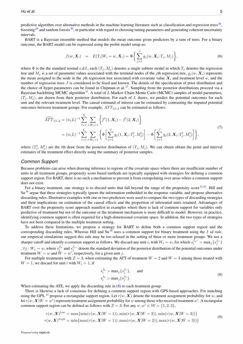
Distributions of estimated GPSs across the treatments are compared using boxplots. For each overlap scenario, weestimated the GPS for each unit in the sample using GBM, and plotted the distributions of estimated GPSs using a separateboxplot for the unit receiving each type of treatment (Figure 1). Substantial overlap in boxplots is presented in the strongoverlap scenario, while the weak overlap scenario highlights the different distributions of GPSs.

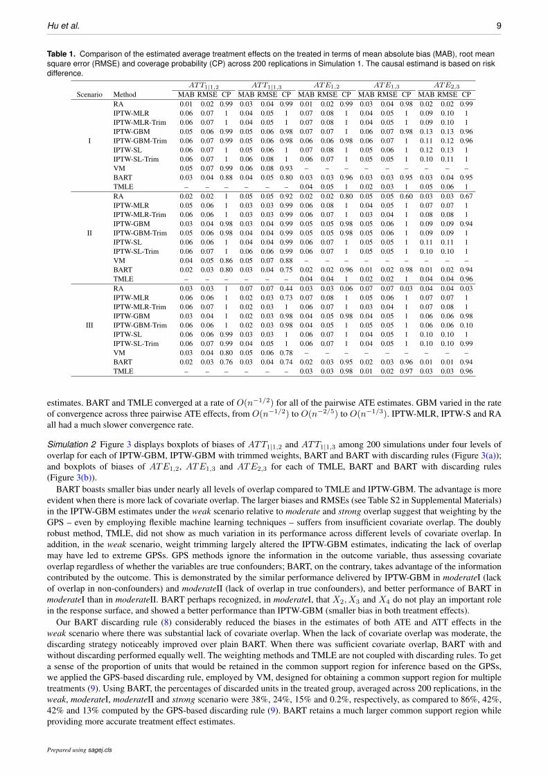
Simulation ResultsSimulation 1 Table 1 displays the MAB, RMSE and CP of the estimates of two ATT effects ATT1|1,2 and ATT1|1,3, andthree ATE effects ATE1,2,ATE1,3 and ATE2,3, for the three scenarios in Simulation 1.

No single method trumped others in estimating both ATT1|1,2 and ATT1|1,3 across all three scenarios. For ATT1|1,2,outcome modeling approaches had smaller MABs and RMSEs, whereas for ATT1|1,3, GPS approaches showed similar or



(a) Weak Covariate Overlap

(b) Moderate Covariate Overlap

(c) Strong Covariate Overlap

Figure 1. Overlap assessment for the scenarios of weak, moderate and strong covariate overlap. Each panel presents boxplots bytreatment group of the estimated generalized propensity scores for one of the treatments, P (Wi = w|X), w ∈ {1, 2, 3}, for everyunit in the sample. The left panel presents treatment 1 (W = 1), the middle panel presents treatment 2 (W = 2), and the rightpanel presents treatment 3 (W = 3).

slightly better performance than BART. RA performed best under the scenario of equal sample sizes. As the sample sizesin the comparison groups grew relative to the reference group, BART generally produced low MAB and RMSE. With GPSapproaches, IPTW-GBM outperformed IPTW-MLR, IPTW-MLR-Trim, IPTW-SL and IPTW-SL-Trim in the estimates ofATT1|1,2 across all three scenarios, but had similar performances in estimating ATT1|1,3. Weight trimming did not improveIPTW-MLR, IPTW-GBM or IPTW-SL. VM presented larger bias and RMSE than BART and IPTW-GBM. None of themethods had nominal CP. IPTW methods and RA in general generated greater than the nominal CP, VM had a CP thatdecreased as the ratio of units became more unbalanced (0.99 to 0.80), and BART yielded a CP around 0.80 – 0.88, whichwe suspect is because the reference group is relatively small. Overall, BART and IPTW-GBM tended to show the bestperformances across settings for the ATT estimates.

For the ATE estimates, BART consistently provided lower MAB and RMSE followed by TMLE, across all three scenarioswith different ratio of units. BART had nominal CP across all three scenarios. IPTW methods and TMLE yielded conservativeintervals and greater than the nominal CP. RA was sensitive to the ratio of units. In the scenario with highly unequalsample sizes across treatment groups, RA had subpar performance. The intervals produced by RA rarely covered the trueeffects, resulting in a low CP. Altogether, BART and TMLE provided the best performances across settings for the ATEestimates. Boxplots of biases from 200 replications in pairwise ATT and ATE estimates appear in Figure S1 and Figure S2in Supplemental Materials.

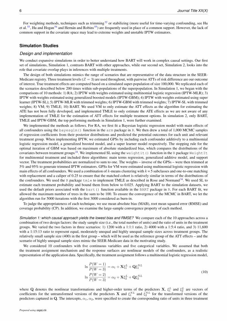
In Figure 2, we examined the large-sample convergence property of each of six methods. We considered only the scenariowith the ratio of units = 1:15:13, which is the most representative of the SEER-Medicare registry. We simulated the datawith increasing sample sizes of n =(2900, 5800, 8700, 11,600, 14,500, 17,400).We computed the RMSE of the estimates ofATT1|1,2 and ATT1|1,3 for each n. We then regressed log(RMSE) on (− log n) using a simple linear regression with a slopeb for each method. The least-squares estimation of b approximates the convergence rate56. BART and GBM converged at arate ofO(n−1/2) for both ATT estimates. IPTW-MLR, IPTW-SL, VM and RA all converged at a slower rate thanO(n−1/2).Figure S3 in Supplemental Materials displays the convergence property of each of six method for the estimates of the ATE


Hu et al. 9

Table 1. Comparison of the estimated average treatment effects on the treated in terms of mean absolute bias (MAB), root meansquare error (RMSE) and coverage probability (CP) across 200 replications in Simulation 1. The causal estimand is based on riskdifference.

ATT1|1,2 ATT1|1,3 ATE1,2 ATE1,3 ATE2,3

Scenario Method MAB RMSE CP MAB RMSE CP MAB RMSE CP MAB RMSE CP MAB RMSE CPRA 0.01 0.02 0.99 0.03 0.04 0.99 0.01 0.02 0.99 0.03 0.04 0.98 0.02 0.02 0.99IPTW-MLR 0.06 0.07 1 0.04 0.05 1 0.07 0.08 1 0.04 0.05 1 0.09 0.10 1IPTW-MLR-Trim 0.06 0.07 1 0.04 0.05 1 0.07 0.08 1 0.04 0.05 1 0.09 0.10 1IPTW-GBM 0.05 0.06 0.99 0.05 0.06 0.98 0.07 0.07 1 0.06 0.07 0.98 0.13 0.13 0.96

I IPTW-GBM-Trim 0.06 0.07 0.99 0.05 0.06 0.98 0.06 0.06 0.98 0.06 0.07 1 0.11 0.12 0.96IPTW-SL 0.06 0.07 1 0.05 0.06 1 0.07 0.08 1 0.05 0.06 1 0.12 0.13 1IPTW-SL-Trim 0.06 0.07 1 0.06 0.08 1 0.06 0.07 1 0.05 0.05 1 0.10 0.11 1VM 0.05 0.07 0.99 0.06 0.08 0.93 – – – – – – – – –BART 0.03 0.04 0.88 0.04 0.05 0.80 0.03 0.03 0.96 0.03 0.03 0.95 0.03 0.04 0.95TMLE – – – – – – 0.04 0.05 1 0.02 0.03 1 0.05 0.06 1RA 0.02 0.02 1 0.05 0.05 0.92 0.02 0.02 0.80 0.05 0.05 0.60 0.03 0.03 0.67IPTW-MLR 0.05 0.06 1 0.03 0.03 0.99 0.06 0.08 1 0.04 0.05 1 0.07 0.07 1IPTW-MLR-Trim 0.06 0.06 1 0.03 0.03 0.99 0.06 0.07 1 0.03 0.04 1 0.08 0.08 1IPTW-GBM 0.03 0.04 0.98 0.03 0.04 0.99 0.05 0.05 0.98 0.05 0.06 1 0.09 0.09 0.94

II IPTW-GBM-Trim 0.05 0.06 0.98 0.04 0.04 0.99 0.05 0.05 0.98 0.05 0.06 1 0.09 0.09 1IPTW-SL 0.06 0.06 1 0.04 0.04 0.99 0.06 0.07 1 0.05 0.05 1 0.11 0.11 1IPTW-SL-Trim 0.06 0.07 1 0.06 0.06 0.99 0.06 0.07 1 0.05 0.05 1 0.10 0.10 1VM 0.04 0.05 0.86 0.05 0.07 0.88 – – – – – – – – –BART 0.02 0.03 0.80 0.03 0.04 0.75 0.02 0.02 0.96 0.01 0.02 0.98 0.01 0.02 0.94TMLE – – – – – – 0.04 0.04 1 0.02 0.02 1 0.04 0.04 0.96RA 0.03 0.03 1 0.07 0.07 0.44 0.03 0.03 0.06 0.07 0.07 0.03 0.04 0.04 0.03IPTW-MLR 0.06 0.06 1 0.02 0.03 0.73 0.07 0.08 1 0.05 0.06 1 0.07 0.07 1IPTW-MLR-Trim 0.06 0.07 1 0.02 0.03 1 0.06 0.07 1 0.03 0.04 1 0.07 0.08 1IPTW-GBM 0.03 0.04 1 0.02 0.03 0.98 0.04 0.05 0.98 0.04 0.05 1 0.06 0.06 0.98

III IPTW-GBM-Trim 0.06 0.06 1 0.02 0.03 0.98 0.04 0.05 1 0.05 0.05 1 0.06 0.06 0.10IPTW-SL 0.06 0.06 0.99 0.03 0.03 1 0.06 0.07 1 0.04 0.05 1 0.10 0.10 1IPTW-SL-Trim 0.06 0.07 0.99 0.04 0.05 1 0.06 0.07 1 0.04 0.05 1 0.10 0.10 0.99VM 0.03 0.04 0.80 0.05 0.06 0.78 – – – – – – – – –BART 0.02 0.03 0.76 0.03 0.04 0.74 0.02 0.03 0.95 0.02 0.03 0.96 0.01 0.01 0.94TMLE – – – – – – 0.03 0.03 0.98 0.01 0.02 0.97 0.03 0.03 0.96

estimates. BART and TMLE converged at a rate of O(n−1/2) for all of the pairwise ATE estimates. GBM varied in the rateof convergence across three pairwise ATE effects, from O(n−1/2) to O(n−2/5) to O(n−1/3). IPTW-MLR, IPTW-S and RAall had a much slower convergence rate.

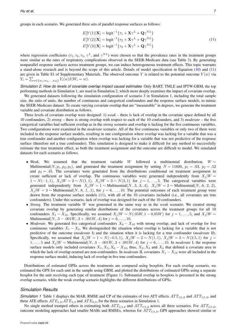
Simulation 2 Figure 3 displays boxplots of biases of ATT1|1,2 and ATT1|1,3 among 200 simulations under four levels ofoverlap for each of IPTW-GBM, IPTW-GBM with trimmed weights, BART and BART with discarding rules (Figure 3(a));and boxplots of biases of ATE1,2, ATE1,3 and ATE2,3 for each of TMLE, BART and BART with discarding rules(Figure 3(b)).

BART boasts smaller bias under nearly all levels of overlap compared to TMLE and IPTW-GBM. The advantage is moreevident when there is more lack of covariate overlap. The larger biases and RMSEs (see Table S2 in Supplemental Materials)in the IPTW-GBM estimates under the weak scenario relative to moderate and strong overlap suggest that weighting by theGPS – even by employing flexible machine learning techniques – suffers from insufficient covariate overlap. The doublyrobust method, TMLE, did not show as much variation in its performance across different levels of covariate overlap. Inaddition, in the weak scenario, weight trimming largely altered the IPTW-GBM estimates, indicating the lack of overlapmay have led to extreme GPSs. GPS methods ignore the information in the outcome variable, thus assessing covariateoverlap regardless of whether the variables are true confounders; BART, on the contrary, takes advantage of the informationcontributed by the outcome. This is demonstrated by the similar performance delivered by IPTW-GBM in moderateI (lackof overlap in non-confounders) and moderateII (lack of overlap in true confounders), and better performance of BART inmoderateI than in moderateII. BART perhaps recognized, in moderateI, that X2, X3 and X4 do not play an important rolein the response surface, and showed a better performance than IPTW-GBM (smaller bias in both treatment effects).

Our BART discarding rule (8) considerably reduced the biases in the estimates of both ATE and ATT effects in theweak scenario where there was substantial lack of covariate overlap. When the lack of covariate overlap was moderate, thediscarding strategy noticeably improved over plain BART. When there was sufficient covariate overlap, BART with andwithout discarding performed equally well. The weighting methods and TMLE are not coupled with discarding rules. To geta sense of the proportion of units that would be retained in the common support region for inference based on the GPSs,we applied the GPS-based discarding rule, employed by VM, designed for obtaining a common support region for multipletreatments (9). Using BART, the percentages of discarded units in the treated group, averaged across 200 replications, in theweak, moderateI, moderateII and strong scenario were 38%, 24%, 15% and 0.2%, respectively, as compared to 86%, 42%,42% and 13% computed by the GPS-based discarding rule (9). BART retains a much larger common support region whileproviding more accurate treatment effect estimates.



Figure 2. The large-sample convergence rate of each of six methods for the estimates of two treatment effects, ATT1|1,2 andATT1|1,3. BART and IPTW-GBM converged the fastest, approximately at a rate of O(n−1/2). RA converged the slowest,approximately at a rate of O(n−1/20).

Application to SEER-Medicare Data on NSCLC

Clinical encounter and Medicare claims data on 11,980 patients with stage I-IIIA NSCLC was drawn from the latest SEER-Medicare database. These patients were above 65 years of age, diagnosed between 2008 (first year patients in the registryunderwent robotic-assisted surgery) and 2013, and underwent surgical resection via one of the three approaches, includingrobotic-assisted surgery, VATS or open thoractomy. The dataset contains individual-level information at baseline on thefollowing variables: age, gender, marital status, race, ethnicity, income level, comorbidities, cancer stage, tumor size, tumorsite, cancer histology and whether they underwent positron emission tomography (PET), chest computer tomography (CT)or mediastinoscopy. Table 2 summarizes these variables for each surgical approach. We compared the effectiveness of thethree surgical approaches in terms of four outcomes: the presence of respiratory complication within 30 days of surgery orduring the hospitalization in which the primary surgical procedure was performed, prolonged length of stay (LOS) (i.e., >14 days), intensive care unit (ICU) stay following surgery and readmission within 30 days of surgery. Table 3 displays theoutcome rates in the three surgical groups.

Among the 11,980 patients, 396 (3.3%) received robotic-assisted surgery, 6582 (54.9%) underwent VATS, and 5002(41.8%) were operated via open thoracotomy. We estimated the causal effects of robotic-assisted surgery vs. VATSor open thoracotomy among patients underwent robotic-assisted surgery (i.e., ATTs1|s1,s2 and ATTs1|s1,s3 ) and in theoverall population (i.e., ATEs1,s2 and ATEs1,s3 ) using BART, regression adjustment, IPTW with GPSs estimated usingmultinomial logistic regression or GBM (with or without trimming), and VM. Each method was implemented as describedin the simulation section. All pre-treatment covariates were included additively to the GPS models for IPTW methods andVM, and to the response surface models for RA and BART.

Table S3 in Supplemental Materials presents the point and interval estimates ofATTs1|s1,s2 andATTs1|s1,s3 based on riskdifference for all the methods examined. To provide uncertainty intervals for the treatment effect estimates, nonparametricbootstrap was used for the IPTW methods and VM, and Bayesian posterior intervals were used for RA and BART. Allmethods yielded statistically insignificant effects on respiratory complication and readmission if patients who receivedrobotic-assisted surgery had instead been treated with open thoracotomy or VATS. For prolonged LOS and ICU stay, allmethods except RA and VM suggested that robotic-assisted surgery led to significant smaller rates of the outcomes comparedto open thoracotomy, but no statistically significant differences compared to VATS. The results from this empirical datasetprovided partial evidence that robotic-assisted surgery may have a positive effect on some postoperative outcomes amongthose who were operated with robotic-assisted surgery compared to open resection, but no advantages on over VATS.

To highlight the importance of simultaneous comparisons of multiple treatments, we implemented each method usingSBC to show how such inappropriate practices can result in different and confusing estimates of treatment effects. Table S3


Hu et al. 11

(a) BART-discard vs. GBM for ATT estimates

(b) BART-discard vs. TMLE for ATE estimates

Figure 3. Biases among 200 replications under scenarios of differing covariate overlap for IPTW-GBM vs. BART and two treatmenteffects ATT1|1,2 and ATT1|1,3; and for TMLE vs. BART and three treatment effects ATE1,2, ATE1,3 and ATE2,3.

also includes the estimates of ATTs1|s1,s2 and ATTs1|s1,s3 from SBC. For BART, the conclusions are generally consistentwith those using multiple treatment comparisons, though we note several inconsistent directions of the estimates of treatmenteffects. Given the different estimands and subpopulations to which inference using SBC is generalizable when using GPS-based approaches, it would generally be inappropriate to directly compare causal estimates. However, we note that IPTWmethods, implemented using SBC, did not always match the findings that were based on IPTW methods designed for multipletreatments. Details appear in Table S4 in Supplementary Materials.

We further explored the sensitivity of BART for binary outcomes to the choice of end-node prior, specifically via thehyperparameter k 40. We employed 5-fold cross-validation to choose the optimal k that minimizes the misclassification error.Results suggested the optimal hyperparameter k = 2, which is the default value of k in the bart() function (not shown).Moreover, we extended the 1 sd rule, the discarding rule of BART proposed by Hill and Su39, to the multiple treatmentsetting, to assess whether common support between treatment groups is reasonable based on the uncertainty in the posterior



Table 2. Baseline characteristics of patients in three surgical groups in SEER-Medicare data.Robotic-Assisted Surgery VATS Open Thoracotomy

Characteristics N = 396 N = 6582 N = 5002

Age (years), mean (SD) 74.3 (5.7) 73.9 (5.4) 74.5 (5.7)Female, N (%) 223 (56.3) 3446 (52.4) 2941 (58.8)Married, N (%) 227 (57.3) 3753 (57.0) 2802 (56.0)Race, N (%)

White 320 (80.8) 5694 (86.5) 4369 (87.3)Black 21 (5.3) 364 (5.5) 248 (5.0)Hispanic 15 (3.8) 218 (3.3) 139 (2.8)Other 40 (10.1) 306 (4.6) 246 (4.9)

Median household annual income, N (%)1st quartile 97 (24.5) 2132 (32.4) 1009 (20.2)2nd quartile 88 (22.2) 1729 (26.3) 1193 (23.9)3rd quartile 98 (24.7) 1345 (20.4) 1143 (22.9)4th quartile 113 (28.5) 1376 (20.9) 1657 (33.1)

Charlson comorbidity score, N (%)0− 1 154 (38.9) 2163 (32.9) 1810 (36.2)1− 2 113 (28.5) 1944 (29.5) 1379 (27.6)> 2 129 (32.6) 2475 (37.6) 1813 (36.2)

Year of diagnosis, N (%)2008-2009 14(3.5) 2686 (40.8) 1484 (29.7)2010 33 (8.3) 1123 (17.1) 857 (17.1)2011 85 (21.5) 1033 (15.7) 866 (17.3)2012 131 (33.1) 899 (13.7) 821 (16.4)2013 133 (33.6) 841 (12.8) 974 (19.5)

Cancer stage, N (%)Stage I 295 (74.5) 4195 (63.7) 3884 (77.6)Stage II 63 (15.9) 1504 (22.9) 709 (14.2)Stage IIIA 38 (9.6) 883 (13.4) 409 (8.2)

Tumor size, in mm, N (%)≤ 20 160 (40.4) 1967 (29.9) 2232 (44.6)21− 30 98 (24.7) 1696 (25.8) 1388 (27.7)31− 50 109 (27.5) 1804 (27.4) 987 (19.7)≥ 51 29 (7.3) 1084 (16.5) 367 (7.3)

Histology, N (%)Adenocarcinoma 255 (64.4) 3757 (57.1) 3348 (66.9)Squamous cell carcinoma 107 (27.0) 2165 (32.9) 1167 (23.3)Other histology 34 (8.6) 660 (10.0) 487 (9.7)

Tumor site, N (%)Upper lobe 215 (54.3) 3829 (58.2) 2859 (57.2)Middle lobe 27 (6.8) 308 (4.7) 335 (6.7)Lower lobe 141 (35.6) 2195 (33.3) 1720 (34.4)Other site 13 (3.3) 250 (3.8) 88 (1.8)

PET scan, N (%) 302 (76.3) 5004 (76.0) 3410 (68.2)Chest CT, N (%) 263 (66.4) 4525 (68.7) 3148 (62.9)Mediastinoscopy, N (%) 62 (15.7) 715 (10.9) 420 (8.4)

Abbreviations: PET = positron emission tomography; SD = standard deviation; CT = computer tomography

Table 3. The outcome rates in three surgical groups: robotic-assisted surgery, VATS and open thoracotomy.Outcomes Robotic-Assisted Surgery VATS Open Thoracotomy Overall

N = 396 N = 6582 N = 5002 N = 11960

Respiratory complication 30.1% 33.6% 33.3% 33.3%Prolonged LOS 5.3% 10.4% 5.5% 8.2%ICU Stay 60.2% 75.3% 59.1% 67.9%Readmission 8.8% 9.8% 8.0% 9.0%

predictive distributions associated with the outcome in the observed versus the counter-factual treatment group. We did notexclude any patients from the empirical dataset based on the discarding rule in (8).

Summary and DiscussionOur paper makes two primary contributions to the causal inference literature. First, we extend BART to the multipletreatment and binary outcome setting, highlighting that the strengths of BART for binary treatment also manifest withmultiple treatments. Second, we propose a common support rule for BART, and find that BART consistently shows superiorperformance over alternative approaches in various scenarios with differing levels of covariate overlap.

In addition to the primary findings in our simulations corresponding to bias, RMSE, CP and large-sample convergenceproperty. BART boasts a few additional advantages that make it a unique tool for the multiple treatment setting. As one


Hu et al. 13

example, BART is computationally efficient. All simulations were run in R on a iMAC with a 4GHz Intel Core i7 processor.On a dataset of size n=11,600, each BART implementation took less than 150 seconds to run, while each IPTW-GBMimplentation took about 10 minutes to run. As a second example, BART produces coherent interval estimates of the treatmenteffects for either continuous or binary outcomes using posterior samples. For GBM, McCaffrey et al.24 estimate the varianceby using robust procedure for continuous outcomes, but acknowledge that there is currently lack of theory to guarantee thatthis approach results in proper confidence intervals. For estimands based on a binary outcome such as the risk differenceinvestigated in this article, it is difficult to approximate the variance using robust procedure. For matching based approaches,there is still ambiguity regarding appropriate methods for interval estimation14,20,38.

We apply the methods examined to 11,980 stage I-IIIA NSCLC patients, drawn from the latest SEER-Medicare linkage.Results suggest that robotic-assisted surgery may be preferred in terms of prolonged LOS and ICU stay, among those whowere operated via the robotic-assisted technology, relative to open thoracotomy or VATS. Different choice of methods,or inappropriate practice such as implementing SBC for pairwise ATT effects, may lead to different conclusions aboutthe treatment effects, explicating the importance of appropriate methods and practice for causal inference with multipletreatments.

The promising performance of BART in the complex multiple treatment settings will lay groundwork for several futureresearch avenues. First, the flexibility offered by nonparametric modeling of BART can be leveraged to model regressionrelationships in survival data. Second, individual treatment effects that are easily obtained from BART provide a buildingblock for estimating the heterogeneous treatment effect. Finally, we have made a significant untestable assumption related tounmeasured confounding. Developing sensitivity analyses under this complex multiple treatments setting leveraging BARTwould also be a worthwhile and important contribution.

Acknowledgements

This study used the linked SEER-Medicare database. The interpretation and reporting of these data are the sole responsibility of theauthors. The authors acknowledge the efforts of the National Cancer Institute; the Office of Research, Development and Information, CMS;Information Management Services (IMS), Inc.; and the Surveillance, Epidemiology, and End Results (SEER) Program tumor registries inthe creation of the SEER-Medicare database.

Funding

This work was supported in part by award ME 2017C3 9041 from the Patient-Centered Outcomes Research Institute, and by grantP30CA196521-01 from the National Cancer Institute.

References

1. Ferlay J et al. Global cancer observatory: Cancer tomorrow. Lyon, France: International Agency for Research on Cancer. https://gco.iarc.fr/tomorrow, 2018. Accessed October 13, 2018.

2. Molina JR, Yang P, Cassivi SD et al. Non-small cell lung cancer: epidemiology, risk factors, treatment, and survivorship. Mayo ClinicProceedings 2008; 83(5): 584–594.

3. Uramoto H and Tanaka F. Recurrence after surgery in patients with nsclc. Translational Lung Cancer Research 2014; 3(4): 242–249.4. Scott WJ, Matteotti RS, Egleston BL et al. A comparison of perioperative outcomes of video-assisted thoracic surgical (vats)

lobectomy with open thoracotomy and lobectomy: results of an analysis using propensity score based weighting. Annals of SurgicalInnovation and Research 2010; 4(1): 1.

5. Whitson BA, Groth SS, Duval SJ et al. Surgery for early-stage non-small cell lung cancer: a systematic review of the video-assistedthoracoscopic surgery versus thoracotomy approaches to lobectomy. The Annals of Thoracic Surgery 2008; 86(6): 2008–2018.

6. Park BJ, Melfi F, Mussi A et al. Robotic lobectomy for non–small cell lung cancer (nsclc): long-term oncologic results. The Journalof Thoracic and Cardiovascular Surgery 2012; 143(2): 383–389.

7. Wisnivesky JP, Smith CB, Packer S et al. Survival and risk of adverse events in older patients receiving postoperative adjuvantchemotherapy for resected stages ii-iiia lung cancer: observational cohort study. BMJ 2011; 343: d4013.

8. Yan TD, Black D, Bannon PG et al. Systematic review and meta-analysis of randomized and nonrandomized trials on safety andefficacy of video-assisted thoracic surgery lobectomy for early-stage non-small-cell lung cancer. Journal of Clinical Oncology 2009;27(15): 2553–2562.

9. Toker A. Robotic thoracic surgery: from the perspectives of european chest surgeons. Journal of Thoracic Disease 2014; 6(Suppl 2):S211–S216.

10. Cajipe MD, Chu D, Bakaeen FG et al. Video-assisted thoracoscopic lobectomy is associated with better perioperative outcomes thanopen lobectomy in a veteran population. The American Journal of Surgery 2012; 204(5): 607–612.

11. Warren JL, Klabunde CN, Schrag D et al. Overview of the seer-medicare data: content, research applications, and generalizability tothe united states elderly population. Medical Care 2002; 40(8): IV3–IV18.

12. Veluswamy RR, Whittaker SA, Nicastri DG et al. Comparative effectiveness of robotic-assisted surgery for resectable lung cancer inolder patients. American Journal of Respiratory and Critical Care Medicine 2017; 195: A4884.

13. Wisnivesky JP, Henschke CI, Swanson S et al. Limited resection for the treatment of patients with stage ia lung cancer. Annals ofSurgery 2010; 251(3): 550–554.


https://gco.iarc.fr/tomorrow

https://gco.iarc.fr/tomorrow


14. Lopez MJ and Gutman R. Estimation of causal effects with multiple treatments: a review and new ideas. Statistical Science 2017;32(3): 432–454.

15. Agresti A. Categorical Data Analysis. John Wiley & Sons, 2003.16. Austin PC. The performance of different propensity score methods for estimating marginal odds ratios. Statistics in Medicine 2007;

26(16): 3078–3094.17. Austin PC. The performance of different propensity-score methods for estimating relative risks. Journal of Clinical Epidemiology

2008; 61(6): 537–545.18. Austin PC. The performance of different propensity-score methods for estimating differences in proportions (risk differences or

absolute risk reductions) in observational studies. Statistics in Medicine 2010; 29(20): 2137–2148.19. Imbens GW. The role of the propensity score in estimating dose-response functions. Biometrika 2000; 87(3): 706–710.20. Imai K and Van Dyk DA. Causal inference with general treatment regimes: Generalizing the propensity score. Journal of the American

Statistical Association 2004; 99(467): 854–866.21. Rosenbaum PR and Rubin DB. The central role of the propensity score in observational studies for causal effects. Biometrika 1983;

70(1): 41–55.22. Linden A, Uysal SD, Ryan A et al. Estimating causal effects for multivalued treatments: a comparison of approaches. Statistics in

Medicine 2016; 35(4): 534–552.23. Feng P, Zhou XH, Zou QM et al. Generalized propensity score for estimating the average treatment effect of multiple treatments.

Statistics in Medicine 2012; 31(7): 681–697.24. McCaffrey DF, Griffin BA, Almirall D et al. A tutorial on propensity score estimation for multiple treatments using generalized

boosted models. Statistics in Medicine 2013; 32(19): 3388–3414.25. Rubin DB. The use of matched sampling and regression adjustment to remove bias in observational studies. Biometrics 1973; 29(1):

185–203.26. Rubin DB. Using multivariate matched sampling and regression adjustment to control bias in observational studies. Journal of the

American Statistical Association 1979; 74(366a): 318–328.27. Imbens GW and Rubin DB. Causal Inference in Statistics, Social, and Biomedical Sciences. Cambridge University Press, 2015.28. Horvitz DG and Thompson DJ. A generalization of sampling without replacement from a finite universe. Journal of the American

Statistical Association 1952; 47(260): 663–685.29. Little RJ. Missing-data adjustments in large surveys. Journal of Business & Economic Statistics 1988; 6(3): 287–296.30. Kang JD, Schafer JL et al. Demystifying double robustness: A comparison of alternative strategies for estimating a population mean

from incomplete data. Statistical Science 2007; 22(4): 523–539.31. Cole SR and Hernan MA. Constructing inverse probability weights for marginal structural models. American journal of epidemiology

2008; 168(6): 656–664.32. Lee BK, Lessler J and Stuart EA. Weight trimming and propensity score weighting. PloS One 2011; 6(3): e18174.33. Van der Laan MJ, Polley EC and Hubbard AE. Super learner. Statistical Applications in Genetics and Molecular Biology 2007; 6(1).34. Rose S and Normand SL. Double robust estimation for multiple unordered treatments and clustered observations: Evaluating drug-

eluting coronary artery stents. Biometrics 2019; 75(1): 289–296.35. Schuler MS and Rose S. Targeted maximum likelihood estimation for causal inference in observational studies. American Journal of

Epidemiology 2017; 185(1): 65–73.36. Chipman HA, George EI and Mcculloch RE. Bayesian ensemble learning. In Scholkopf B, Platt JC and Hoffman T (eds.) Advances

in Neural Information Processing Systems 19. MIT Press, 2007. pp. 265–272. URL http://papers.nips.cc/paper/

3084-bayesian-ensemble-learning.pdf.37. Chipman HA, George EI, McCulloch RE et al. Bart: Bayesian additive regression trees. The Annals of Applied Statistics 2010; 4(1):

266–298.38. Hill JL. Bayesian nonparametric modeling for causal inference. Journal of Computational and Graphical Statistics 2011; 20(1):

217–240.39. Hill J and Su YS. Assessing lack of common support in causal inference using bayesian nonparametrics: Implications for evaluating

the effect of breastfeeding on children’s cognitive outcomes. The Annals of Applied Statistics 2013; 7(3): 1386–1420.40. Dorie V, Harada M, Carnegie NB et al. A flexible, interpretable framework for assessing sensitivity to unmeasured confounding.

Statistics in Medicine 2016; 35(20): 3453–3470.41. Neyman J. On the application of probability theory to agricultural experiments. essay on principles. section 9. portions translated into

english by d. dabrowska and t. speed (1990). Statistical Science 1923; 5(4): 465–472.42. Rubin DB. Estimating causal effects of treatments in randomized and nonrandomized studies. Journal of Educational Psychology

1974; 66(5): 688–701.43. Rubin DB. Assignment to treatment group on the basis of a covariate. Journal of Educational Statistics 1977; 2(1): 1–26.44. Rubin DB. Bayesian inference for causal effects: The role of randomization. The Annals of Statistics 1978; 6(1): 34–58.45. Holland PW. Statistics and causal inference. Journal of the American Statistical Association 1986; 81(396): 945–960.46. Rubin DB. Randomization analysis of experimental data: The fisher randomization test comment. Journal of the American Statistical

Association 1980; 75(371): 591–593.47. Ding P and Li F. Causal inference: A missing data perspective. Statistical Science 2018; 33(2): 214–237.48. Breiman L, Friedman J, Stone CJ et al. Classification and Regression Trees. CRC press, 1984.


http://papers.nips.cc/paper/3084-bayesian-ensemble-learning.pdf

http://papers.nips.cc/paper/3084-bayesian-ensemble-learning.pdf

Hu et al. 15

49. Freund Y and Schapire RE. A desicion-theoretic generalization of on-line learning and an application to boosting. Journal ofComputer and System Sciences 1997; 55: 119–139.

50. Breiman L. Random forests. Machine Learning 2001; 45(1): 5–32.51. Dehejia RH and Wahba S. Propensity score-matching methods for nonexperimental causal studies. Review of Economics and Statistics

2002; 84(1): 151–161.52. Morgan SL and Harding DJ. Matching estimators of causal effects: Prospects and pitfalls in theory and practice. Sociological Methods

& Research 2006; 35(1): 3–60.53. Hu L, Hogan JW, Mwangi AW et al. Modeling the causal effect of treatment initiation time on survival: Application to HIV/TB

co-infection. Biometrics 2018; 74(2): 703–713.54. Hu L and Hogan JW. Causal comparative effectiveness analysis of dynamic continuous-time treatment initiation rules with sparsely

measured outcomes and death. Biometrics 2019; 75(2): 695–707.55. Hernan M and Robins J. Causal Inference. Boca Raton: Chapman & Hall/CRC, forthcoming, 2019.56. Liu T, Hogan JW, Wang L et al. Optimal allocation of gold standard testing under constrained availability: application to assessment

of HIV treatment failure. Journal of the American Statistical Association 2013; 108(504): 1173–1188.


liangyuan hu1,2,3, chenyang gu4, michael lopez5, jiayi ji

Documents