Lecture 4: Analysis of Optimal Trajectories,

Transition Dynamics in Growth Model

ECO 503: Macroeconomic Theory I

Benjamin Moll

Princeton University

Fall 2014

1 / 30

Plan of Lecture

1 Linearization around steady state, speed of convergence,slope of saddle path

2 Some transition experiments in the growth model

2 / 30

Linearization around Steady State

• Two questions:

• can we say more than “there exists a unique steady state andthe economy converges to it”? Speed of convergence?

• How analyze stability if two- or N-dimensional state x (so thatcannot draw phase diagram)?

• Can answer these questions by analyzing local dynamics closeto steady state

3 / 30

Linearization around Steady State• Let y ∈ Rn and the function m : Rn → Rn define a dynamical

system:y (t) = m(y(t)) for t ≥ 0,

• Let y∗ be a steady state, i.e. 0 = m (y∗)

• Consider a first order approximation of m around y∗ :

y ≈ m(y∗) + m′ (y∗) (y − y∗)

where m′(y∗) is the n × n Jacobian of m evaluated at y∗, i.e.the matrix with entries ∂mi (y

∗)/∂yj• Equivalently

˙y ≈ Ay , y = y − y∗, A = m′(y∗)

• Idea is then to analyze this linear differential equation.

• Analysis is valid globally (i.e. for all Rn) if the system isindeed linear.

• Alternatively it is valid in a neighborhood of the steady state.4 / 30

Linearized Growth Model

• Recall system of two ODEs

c =1

σ(f ′(k)− ρ− δ)c

k = f (k)− δk − c(ODE”)

• Let y = (c , k) and do analysis on previous slide

˙y ≈ Ay , A =

[∂c/∂c ∂c/∂k

∂k/∂c ∂k/∂k

], y =

[c − c∗

k − k∗

]where the partial derivatives are evaluated at (c∗, k∗)

• Have

A =

[∂c/∂c ∂c/∂k

∂k/∂c ∂k/∂k

]=

[0 1

σ f′′(k∗)c∗

−1 ρ

]

where we used ∂k/∂k = f ′(k∗)− δ = ρ

5 / 30

Properties of Linear Systems• Theorem (see e.g. Acemoglu, Theorem 7.18) Consider the

following linear differential equation system

˙y (t) = Ay (t) , y = y − y∗ (∗)with initial value y(0), and where A is an n × n matrix.Suppose that ` ≤ n of the eigenvalues of A have negative realparts. Then, there exists an `-dimensional subspace L of Rn

such that that starting from any y(0) ∈ L, the differentialequation (∗) has a unique solution with y(t)→ 0.

• Proof: next slide

• Interpretation: important thing is to compare number ofnegative eigenvalues ` and number of pre-determined statevariables m

• if ` = m (standard case): “saddle-path stable”, unique optimaltrajectory. Neg. eigenvalues govern speed of convergence.

• if ` < m: unstable, y(t) does not converge to steady state.

• if ` > m: multiple optimal trajectories (“indeterminacy”) 6 / 30

Proof of Theorem• First step is to solve (∗). Also see

http://en.wikipedia.org/wiki/Matrix_differential_equation

• Denote the eigenvalues of A by λ1, ..., λn and thecorresponding eigenvectors by v1, ..., vn.

• Diagonalizing the matrix A we obtain:

A = PΛP−1

• Λ is diagonal matrix with eigenvalues of A, possibly complex,on its diagonal.

• Matrix P contains the eigenvectors of A, i.e. P = (v1, ..., vn)(to see this write AP = PΛ or Avi = λivi ) and is invertible

• ignores some technicalities discussed in ch. 6 of SLP book

• Write system as

P−1 ˙y (t) = ΛP−1y (t)

⇔ z (t) = Λz (t) , z(t) = P−1y(t)7 / 30

Proof of Theorem

• Since Λ is diagonal zi = λizi (t), i = 1, ..., n, i.e. it can besolved element by element

zi (t) = cieλi t

where ci are constants of integration

• We have that y(t) = Pz(t). Using P = (v1, ..., vn) we have

y(t) =n∑

i=1

cieλi tvi (∗∗)

• For now, assume all λi are real

• Let λi be such that for i = 1, 2, .., ` we have λi < 0 and fori = `+ 1, `+ 2, ..., n we have λi ≥ 0. That is, eigenvalues ofA are ordered so that first ` are negative.

8 / 30

Proof of Theorem

• Q: when does y(t)→ 0? A: initial condition needs to satisfy

y(0) =n∑

i=1

civi , ci = 0, i = `+ 1, `+ 2, ..., n

• That is, y(t)→ 0 only if y(0) lies in particular subspace ofRn. Dimension of subspace = # of negative eigenvalues `.

• Exercise: how extend to case where λi can be complex?

9 / 30

Linearized Growth Model• Recall

˙y ≈ Ay , A =

[0 1

σ f′′(k∗)c∗

−1 ρ

], y =

[c − c∗

k − k∗

]• Let’s look at eigenvalues of A. These satisfy

0 = det(A− λI ) = −λ(ρ− λ) +1

σf ′′(k∗)c∗

0 = λ2 − ρλ+1

σf ′′(k∗)c∗

• This is a simple quadratic with two solutions (“roots”)

λ1/2 =ρ±

√ρ2 − 4 1

σ f′′(k∗)c∗

2

• f ′′(k∗) < 0 so both eigenvalues are real, and λ1 < 0 < λ2

• Have one pre-determined state variable.

• Theorem says: ` = m = 1 ⇒ saddle-path stable10 / 30

Linearized Growth Model• What does this tell us about the time path of capital k(t)?

• From (∗∗), solution to matrix differential equation for growthmodel is [

y1(t)y2(t)

]≈ c1e

λ1t

[v11v12

]+ c2e

λ2t

[v21v22

]where y1 = c(t)− c∗, y2 = k(t)− k∗ and vi1, vi2 denoteelements of vi

• λ2 > 0⇒ need c2 = 0

c(t)− c∗ ≈ c1eλ1tv11, k(t)− k∗ ≈ c1e

λ1tv12

• Have initial condition for k(0) = k0 ⇒ c1v11 = k0 − k∗

c(t)− c∗ ≈ v11v12

eλ1t(k0 − k∗) (1)

k(t)− k∗ ≈ eλ1t(k0 − k∗) (2)

• From (2), know approximate time path for k(t)• (1) pins down initial consumption (v11 and v12 are known) 11 / 30

Linearization: Speed of Convergence• Negative eigenvalue λ1 governs speed of convergence

k(t)− k∗ ≈ e−|λ1|t(k0 − k∗)

• Half-life for convergence to steady state

k(t1/2)− k∗ =1

2(k0 − k∗) ⇒ t1/2 =

ln(2)

|λ1|• Formula from previous slide:

λ1 =ρ−

√ρ2 − 4 1

σ f′′(k∗)c∗

2• Convergence fast (|λ1| large) if

• high f ′′ (strongly diminishing returns)

• low σ (utility ≈ linear, high “intertemp. elasticity of substit.”)

• Will show later: for reasonable parameter values, neoclassicalgrowth model features very fast speed of convergence, e.g.something like t1/2 = 5 years.

12 / 30

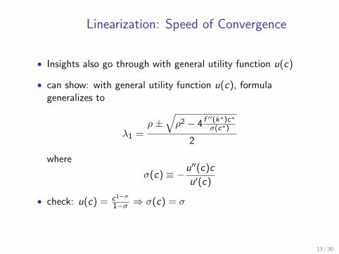
Linearization: Speed of Convergence

• Insights also go through with general utility function u(c)

• can show: with general utility function u(c), formulageneralizes to

λ1 =ρ±

√ρ2 − 4 f ′′(k∗)c∗

σ(c∗)

2

where

σ(c) ≡ −u′′(c)c

u′(c)

• check: u(c) = c1−σ

1−σ ⇒ σ(c) = σ

13 / 30

Slope of Saddle Path

• Recall conditions for optimum:

c

c=

1

σ(f ′(k)− ρ− δ)

k = f (k)− δk − c(ODE”)

with k(0) = k0 and limT→∞ e−ρT c(T )−σk(T ) = 0.

• Saddle path c(k) defines optimal consumption for each k

• a.k.a. consumption policy function

• For many questions, useful to know slope of saddle path

14 / 30

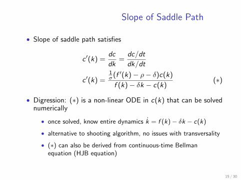
Slope of Saddle Path

• Slope of saddle path satisfies

c ′(k) =dc

dk=

dc/dt

dk/dt

c ′(k) =1σ (f ′(k)− ρ− δ)c(k)

f (k)− δk − c(k)(∗)

• Digression: (∗) is a non-linear ODE in c(k) that can be solvednumerically

• once solved, know entire dynamics k = f (k)− δk − c(k)

• alternative to shooting algorithm, no issues with transversality

• (∗) can also be derived from continuous-time Bellmanequation (HJB equation)

15 / 30

Slope of Saddle Path• Now consider slope of saddle path at steady state c ′(k∗)

c ′(k∗) = limk→k∗

c ′(k) = limk→k∗

1σ (f ′(k)− ρ− δ)c(k)

f (k)− δk − c(k)=

=1σ f′′(k∗)c∗

f ′(k∗)− δ − c ′(k∗)=

1σ f′′(k∗)c∗

ρ− c ′(k∗)

where the third equality follows from L’Hopital’s rule(http://en.wikipedia.org/wiki/L’H%C3%B4pital’s_rule)

• Rearranging, we see that λ = c ′(k∗) satisfies

−λ(ρ− λ) +1

σf ′′(k∗)c∗ = 0

• Same quadratic as before. Two solutions (“roots”)

λ1/2 =ρ±

√ρ2 − 4 1

σ f′′(k∗)c∗

2, λ1 < 0 < λ2

16 / 30

Slope of Saddle Path

• Know c ′(k∗) > 0⇒ slope of saddle path = positive root

c ′(k∗) =ρ+

√ρ2 − 4 1

σ f′′(k∗)c∗

2

• In growth model

• negative eigenvalue of linearized system = speed ofconvergence

• positive eigenvalue of linearized system = slope of saddle path

• seems to be a coincidence, same not true in more generalmodels. Instead slope of saddle path related to eigenvectors.

17 / 30

Linearization and Perturbation: Relation

• Popular method in economics: perturbation methods

• Some useful references:

• Judd (1996) “Approximation, perturbation, and projectionmethods in economic analysis”, Judd’s (1998) book

• Schmitt-Grohe and Uribe (2004)

• Fernandez-Villaverde lecture notes http://economics.sas.

upenn.edu/~jesusfv/Chapter_2_Perturbation.pdf

• Original references from math literature: Fleming (1971),Fleming and Souganidis (1986)

• Takeaway: linearization around steady state is particularapplication of first-order perturbation method

• Why perturbation? Perturbation methods are more generaland there are more powerful theorems

18 / 30

Linearization and Perturbation: Relation• Recall dynamical system from beginning of lecture

y(t) = m(y(t)), y(0) = y0 (∗)• In general, to apply perturbation method need:

1 some known solution of equation, call it y0(t)

2 to express equation as a perturbed version of known solution interms of scalar “perturbation parameter”, call it ε

• Application to our system (∗):

1 know solution if initial condition is steady state, y0 = y∗

2 view (∗) as

y(t, ε) = m(y(t, ε)), y(0, ε) = y∗ + εy0 (∗∗)where εy0 is initial deviation from steady state

• Key idea of perturbation: look for solution of (∗∗) of form

y(t, ε) = y∗ + εy1(t) + ε2y2(t) + ...

• First-order perturbation: y(t, ε) ≈ y∗ + εy1(t)19 / 30

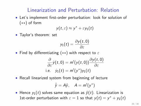
Linearization and Perturbation: Relation• Let’s implement first-order perturbation: look for solution of

(∗∗) of formy(t, ε) ≈ y∗ + εy1(t)

• Taylor’s theorem: set

y1(t) =∂y(t, 0)

∂ε

• Find by differentiating (∗∗) with respect to ε

∂

∂εy(t, 0) = m′(y(t, 0))

∂y(t, 0)

∂εi.e. y1(t) = m′(y∗)y1(t)

• Recall linearized system from beginning of lecture

˙y = Ay , A = m′(y∗)

• Hence y1(t) solves same equation as y(t). Linearization is1st-order perturbation with ε = 1 so that y(t) = y∗ + y1(t)

20 / 30

Linearization: Discrete Time

• Similar results apply for discrete-time optimal controlproblems

• Main difference: it’s about whether eigenvalues are < 1rather than < 0.

• See Stokey-Lucas-Prescott chapter 6.

• Let y ∈ Rn and the function m : Rn → Rn define a dynamicalsystem:

yt+1 = m (yt)

• Let y∗ be a steady state, i.e. y∗ = m (y∗)

• Consider a first order approximation of m around y∗ :

yt+1 ≈ m(y∗) + m′ (y∗) (yt − y∗)

yt+1 ≈ Ayt , yt = yt − y∗, A = m′(y∗),

21 / 30

Linearization: Discrete Time

• Theorem Consider the following linear difference equationsystem

yt+1 = Ayt , yt = yt − y∗ (∗)

with initial value y(0), and where A is an n × n matrix.Suppose that ` ≤ n of the eigenvalues of A have real partsthat are less than one. Then, there exists an `-dimensionalsubspace L of Rn such that that starting from any y0 ∈ L, thedifference equation (∗) has a unique solution with yt → 0.

• Proof is exact analogue

• My advice: if you want to linearize a model/do stabilityanalysis, do it in continuous time

• always works out more nicely

• but be my guest and linearize growth model in discrete time

22 / 30

Transition Experiments

• Consider growth model with utility and production functions

u(c) =c1−σ

1− σ, f (k) = εkα

• Consider following thought experiment

• up until t = 0, economy in steady state

• at t = 0, ε increases permanently to ε′ > ε

• Question: what can we say about time paths of k(t), i(t) andparticularly c(t) as model converges to new steady state?

• consumption increases in long-run, but what about short-run?

23 / 30

Steady State Effects

• For given ε, steady state capital and consumption are

k∗ =

(αε

ρ+ δ

) 11−α

, c∗ = ε(k∗)α − δk∗

• So both k∗ and c∗ increase. Note also that

c∗

k∗= ε(k∗)α−1 − δ =

ρ+ δ

α− δ

which is independent of ε

• But what about transition?

• see phase diagrams on next slides

24 / 30

Case 1: slope of saddle path < c∗/k∗

consumption increases on impact

25 / 30

Case 2: slope of saddle path < c∗/k∗

consumption decreases on impact

26 / 30

Intuition: income vs. substitution effect

• Why can consumption decrease on impact?

• Offsetting income and substitution effects

• income effect: ε ↑⇒ wealthier (PDV or earnings higher)⇒ eat more

• substitution effect: ε ↑⇒ MPK ↑ = return to saving ↑⇒ eat less

• In general, overall effect is ambiguous

• “Income vs. substitution effect” is always the right answer!

27 / 30

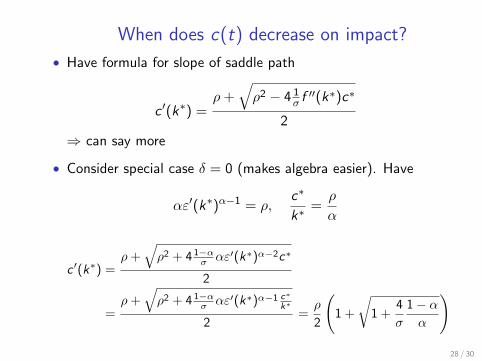
When does c(t) decrease on impact?

• Have formula for slope of saddle path

c ′(k∗) =ρ+

√ρ2 − 4 1

σ f′′(k∗)c∗

2

⇒ can say more

• Consider special case δ = 0 (makes algebra easier). Have

αε′(k∗)α−1 = ρ,c∗

k∗=ρ

α

c ′(k∗) =ρ+

√ρ2 + 4 1−α

σ αε′(k∗)α−2c∗

2

=ρ+

√ρ2 + 4 1−α

σ αε′(k∗)α−1 c∗

k∗

2=ρ

2

(1 +

√1 +

4

σ

1− αα

)28 / 30

When does c(t) decrease on impact?

• So question is when

c ′(k∗) =ρ

2

(1 +

√1 +

4

σ

1− αα

)>ρ

α=

c∗

k∗√α2 +

4

σ(1− α)α > 2− α

α > σ

• Summary:

• σ > α: income effect dominates ⇒ c(t) increases

• σ < α: subst. effect dominates ⇒ c(t) decreases

• σ = α: income and subst. effects cancel ⇒ c(t) constant

• Exercise: what is the cutoff in general case δ > 0

29 / 30

Transition Experiments

• Exercise: analogous experiments for other parameter values

• increase in ρ

• increase in δ

30 / 30