design and analysis of optimal ascent trajectories for
TRANSCRIPT
Design and Analysis of Optimal Ascent Trajectoriesfor Stratospheric Airships
A DISSERTATION
SUBMITTED TO THE FACULTY OF THE GRADUATE SCHOOL
OF THE UNIVERSITY OF MINNESOTA
BY
Joseph Bernard Mueller
IN PARTIAL FULFILLMENT OF THE REQUIREMENTS
FOR THE DEGREE OF
Doctor of Philosophy
Professor Yiyuan J. Zhao
August, 2013
c© Joseph Bernard Mueller 2013
ALL RIGHTS RESERVED
Acknowledgements
Without a doubt, I have been blessed with amazing opportunities and extraordinary
people in my life. The pursuit of this Ph.D. has been an endeavor that has pushed my
limits in many ways. I am grateful for the opportunity and for the people who have
helped me along the way.
I would first like to extend my sincere gratitude to my advisor, Professor Yiyuan Zhao.
When I met Yiyuan in 1995 as a student in his Flight Mechanics course, he immediately
stood out to me as a deeply intelligent, thoughtful, and above all, compassionate person.
Several years after I graduated, it was Yiyuan who encouraged me to pursue a Ph.D. His
belief in me was contagious, and for that I am truly thankful. His guidance, insight and
patience have been instrumental to my growth as a student, and are greatly appreciated.
My thanks also go to Professor William Garrard. He has served as a second advisor
to me throughout this program, and has been a mentor to me for many years. I sincerely
appreciate his guidance, his sage advice, and the many opportunities that he has given.
I extend my thanks to all of my committee members, including Professor Mihailo
Jovanovic and Professor Demoz Gebre, for their time and valuable feedback.
Thanks go to all of the people and organizations that contributed to the funding of
this research. This includes our Aerospace Engineering Department, the National Sci-
ence Foundation, the Minnesota Space Grant, and the Doctoral Dissertation Fellowship
program.
i

Thanks to my colleagues at Princeton Satellite Systems, for their support and en-
couragement as I worked towards this degree.
Thanks to my family and friends for their constant support and faith. My parents
and siblings have always been a source of strength, which has helped me more than they
know.
And finally, I am deeply grateful to my wife, Jessica, and to our three children. Their
sacrifice and loving support over the last several years has humbled me. I will carry this
gratitude with me always.
ii

Dedication
This thesis is dedicated to my wife, Jessica, and to my three children, Allison, Dominick
and Austin. You renew my strength and give me joy.
iii

Abstract
Stratospheric airships are lighter-than-air (LTA) vehicles that have the potential to
provide a long-duration airborne presence at altitudes of 18-22 km. Designed to operate
on solar power in the calm portion of the lower stratosphere and above all regulated
air traffic and cloud cover, these vehicles represent an emerging platform that resides
between conventional aircraft and low Earth-orbiting (LEO) satellites.
A particular challenge for airship operation is the planning of ascent trajectories, as
the slow moving vehicle must traverse the high wind region of the jet stream. Due to the
large changes in wind speed and direction across altitude and the susceptibility of airship
motion to wind, the trajectory must be carefully planned, preferably optimized, in order
to ensure that the desired station be reached within acceptable performance bounds of
flight time, energy consumption, and lateral excursion. This thesis develops optimal
ascent trajectories for stratospheric airships, examines the structure and sensitivity of
these solutions, and presents a strategy for onboard guidance.
Optimal ascent trajectories are developed that utilize wind energy to achieve minimum-
time and minimum-energy flights. The airship is represented by a three-dimensional
point mass model, and the equations of motion include aerodynamic lift and drag, vec-
tored thrust, added mass effects, and accelerations due to mass flow rate, wind rates, and
Earth rotation. A representative wind profile is developed based on historical meteoro-
logical data and measurements. Trajectory optimization is performed by first defining
an optimal control problem with both terminal and path constraints, then using direct
transcription to develop an approximate nonlinear parameter optimization problem of
finite dimension. Optimal ascent trajectories are determined using SNOPT for a variety
of upwind, downwind, and crosswind launch locations. Results of extensive optimization
solutions illustrate definitive patterns in the ascent path for minimum time flights across
varying launch locations, and show that significant energy savings can be realized with
iv
minimum-energy flights, compared to minimum-time time flights, given small increases
in flight time.
The performance of the optimal trajectories are then studied with respect to solar
energy production during ascent, as well as sensitivity of the solutions to small changes
in drag coefficient and wind model parameters. Results of solar power model simulations
indicate that solar energy is sufficient to power ascent flights, but that significant energy
loss can occur for certain types of trajectories. Sensitivity to the drag and wind model
is approximated through numerical simulations, showing that optimal solutions change
gradually with respect to changing wind and drag parameters and providing deeper
insight into the characteristics of optimal airship flights.
Finally, alternative methods are developed to generate near-optimal ascent trajecto-
ries in a manner suitable for onboard implementation. The structures and characteris-
tics of previously developed minimum-time and minimum-energy ascent trajectories are
used to construct simplified trajectory models, which are efficiently solved in a smaller
numerical optimization problem. Comparison of these alternative solutions to the orig-
inal SNOPT solutions show excellent agreement, suggesting the alternate formulations
are an effective means to develop near-optimal solutions in an onboard setting.
v
Contents
Acknowledgements i
Dedication iii
Abstract iv
List of Tables x
List of Figures xi
1 Introduction 1
1.1 Airships . . . . . . . . . . . . . . . . . . . . . . . . . . . . . . . . . . . . 1
1.2 Applications of Stratospheric Airships . . . . . . . . . . . . . . . . . . . 2
1.3 Challenges in Airship Trjajectory Planning . . . . . . . . . . . . . . . . 3
1.4 Research Contributions . . . . . . . . . . . . . . . . . . . . . . . . . . . 4
1.5 Organization . . . . . . . . . . . . . . . . . . . . . . . . . . . . . . . . . 5
2 Related Work 6
2.1 Overview . . . . . . . . . . . . . . . . . . . . . . . . . . . . . . . . . . . 6
2.2 Design and Feasibility Studies . . . . . . . . . . . . . . . . . . . . . . . . 6
2.3 Feedback Control Methods for Airships . . . . . . . . . . . . . . . . . . 7
2.4 Trajectory Planning Methods for Airships . . . . . . . . . . . . . . . . . 8
vi
3 Modeling 10
3.1 Fundamentals of Airship Operation . . . . . . . . . . . . . . . . . . . . . 10
3.2 Baseline Design . . . . . . . . . . . . . . . . . . . . . . . . . . . . . . . . 11
3.3 Equations of Motion . . . . . . . . . . . . . . . . . . . . . . . . . . . . . 12
1 Kinematic Equations . . . . . . . . . . . . . . . . . . . . . . . . . 12
2 External Forces . . . . . . . . . . . . . . . . . . . . . . . . . . . . 15
3 Dynamics . . . . . . . . . . . . . . . . . . . . . . . . . . . . . . . 17
4 Complete Equations of Motion . . . . . . . . . . . . . . . . . . . 20
5 Dimensional Scaling . . . . . . . . . . . . . . . . . . . . . . . . . 21
6 Assumptions . . . . . . . . . . . . . . . . . . . . . . . . . . . . . 22
3.4 Environment Models . . . . . . . . . . . . . . . . . . . . . . . . . . . . . 24
1 Atmospheric Density . . . . . . . . . . . . . . . . . . . . . . . . . 24
2 Horizontal Wind Model . . . . . . . . . . . . . . . . . . . . . . . 25
3 Wind Model with Altitude Dependence Only . . . . . . . . . . . 26
3.5 Solar Power Generation Model . . . . . . . . . . . . . . . . . . . . . . . 27
1 Hull Geometry . . . . . . . . . . . . . . . . . . . . . . . . . . . . 28
2 Sun Vector . . . . . . . . . . . . . . . . . . . . . . . . . . . . . . 29
3 Solar Flux Through All Panels . . . . . . . . . . . . . . . . . . . 30
4 Remarks . . . . . . . . . . . . . . . . . . . . . . . . . . . . . . . . 33
4 Problem Formulations 35
5 Numerical Solution Methods 38
6 Numerical Solution Results 42
5 Characteristics of Optimal Flights . . . . . . . . . . . . . . . . . 43
6 Time and Energy Tradeoff . . . . . . . . . . . . . . . . . . . . . . 50
7 Effects of Varying Initial Positions . . . . . . . . . . . . . . . . . 53
8 Discussions . . . . . . . . . . . . . . . . . . . . . . . . . . . . . . 56
vii
7 Performance Evaluation of Optimal Solutions 58
7.1 Introduction . . . . . . . . . . . . . . . . . . . . . . . . . . . . . . . . . . 58
7.2 Energy Production Analysis . . . . . . . . . . . . . . . . . . . . . . . . . 59
1 Energy Requirement for Ballast Control . . . . . . . . . . . . . . 61
7.3 Sensitivity Analysis . . . . . . . . . . . . . . . . . . . . . . . . . . . . . . 62
1 Variation in Drag Coefficient . . . . . . . . . . . . . . . . . . . . 63
2 Variation in Peak Wind Magnitude . . . . . . . . . . . . . . . . . 64
7.4 Concluding Remarks . . . . . . . . . . . . . . . . . . . . . . . . . . . . . 67
8 Onboard Guidance Methods 69
8.1 Introduction . . . . . . . . . . . . . . . . . . . . . . . . . . . . . . . . . . 69
8.2 Dynamic Inversion . . . . . . . . . . . . . . . . . . . . . . . . . . . . . . 71
1 Airship Dynamic Model . . . . . . . . . . . . . . . . . . . . . . . 73
2 Nonlinear Dynamic Inversion for Airship Guidance . . . . . . . . 73
3 Outer Loop NDI Control . . . . . . . . . . . . . . . . . . . . . . 74
4 Inner Loop NDI Control . . . . . . . . . . . . . . . . . . . . . . . 75
8.3 Virtual Target and Ascent Cone . . . . . . . . . . . . . . . . . . . . . . 80
8.4 Minimum-Time Ascent . . . . . . . . . . . . . . . . . . . . . . . . . . . . 82
1 Maximum Climb-Rate Ascent . . . . . . . . . . . . . . . . . . . . 83
2 Determining the Virtual Target Location . . . . . . . . . . . . . 84
3 Virtual Target Inside the Ascent Cone, dH ≤ Rc . . . . . . . . . 86
4 Virtual Target Outside the Ascent Cone, dH > Rc . . . . . . . . 91
8.5 Minimum-Energy Ascent . . . . . . . . . . . . . . . . . . . . . . . . . . . 101
1 Minimum-Energy Simple Ascent Profile . . . . . . . . . . . . . . 105
2 Minimum-Energy Winding Ascent Profile, ∆tC = 0 . . . . . . . . 107
3 Minimum-Energy Direct Ascent Profile, ∆tC > 0 . . . . . . . . 112
9 Conclusions 121
9.1 Summary . . . . . . . . . . . . . . . . . . . . . . . . . . . . . . . . . . . 121
viii
9.2 Contributions . . . . . . . . . . . . . . . . . . . . . . . . . . . . . . . . . 123
10 Recommendations for Future Work 125
References 127
Appendix A. Glossary and Acronyms 132
A.1 Glossary . . . . . . . . . . . . . . . . . . . . . . . . . . . . . . . . . . . . 132
A.2 Acronyms . . . . . . . . . . . . . . . . . . . . . . . . . . . . . . . . . . . 132
Appendix B. Wind Prediction Model 134
ix

List of Tables
3.1 Baseline Airship Design Parameters . . . . . . . . . . . . . . . . . . . . 12
6.1 Solution Parameters . . . . . . . . . . . . . . . . . . . . . . . . . . . . . 42
6.2 Problem Bounds . . . . . . . . . . . . . . . . . . . . . . . . . . . . . . . 42
A.1 Acronyms . . . . . . . . . . . . . . . . . . . . . . . . . . . . . . . . . . . 133
x
List of Figures
3.1 Topocentric Coordinate System . . . . . . . . . . . . . . . . . . . . . . . 13
3.2 Airship Velocity in the Local and Wind-Relative Frames . . . . . . . . . 15
3.3 External Forces Acting on the Airship . . . . . . . . . . . . . . . . . . . 16
3.4 Conservation of Linear Momentum . . . . . . . . . . . . . . . . . . . . . 19
3.5 HWM93 Wind Profile over Southern California . . . . . . . . . . . . . . 26
3.6 Sun Position with Respect to Solar Panel . . . . . . . . . . . . . . . . . 31
3.7 Irradiance Variation with Altitude . . . . . . . . . . . . . . . . . . . . . 32
3.8 Normalized Solar Intensity for East-West and North-South Orientations
at Winter, Spring/Fall, Summer, for 0 Deg and 30 Deg Pitch Angles . . 32
6.1 Scenarios 1 & 2, Minimum Time and Fixed-Time / Minimum Energy
Trajectories . . . . . . . . . . . . . . . . . . . . . . . . . . . . . . . . . . 44
6.2 Scenario 1 Minimum-Time Ascent Path . . . . . . . . . . . . . . . . . . 44
6.3 Scenario 2, Control History for Minimum Time Solution . . . . . . . . . 45
6.4 Scenario 2, Selected Time Histories for Minimum Time Solution . . . . . 46
6.5 Scenario 2, Control History for Minimum Energy Solution . . . . . . . . 48
6.6 Scenario 2, Selected Time Histories for Minimum Energy Solution . . . 49
6.7 Scenario 2, Minimum Energy 3D Ascent Trajectory . . . . . . . . . . . . 49
6.8 Scenario 1, Control History for Minimum Energy Solution . . . . . . . . 50
6.9 Scenario 1, Selected Time Histories for Minimum Energy Solution . . . 51
6.10 Scenario 1, Minimum Energy 3D Ascent Trajectory . . . . . . . . . . . . 51
xi
6.11 Scenario 2, Acceleration Components for Minimum Time and Minimum
Energy Solutions . . . . . . . . . . . . . . . . . . . . . . . . . . . . . . . 52
6.12 Scenarios 1 & 2, Energy vs. Time . . . . . . . . . . . . . . . . . . . . . . 52
6.13 Scenario 4, Minimum Time Ascent Trajectories from 100 km Radius . . 54
6.14 Scenario 3, Minimum Time Ascent Trajectories from 10 km Radius . . . 55
6.15 Scenarios 4, Energy & Time vs. Launch Location . . . . . . . . . . . . . 55
7.1 Required and Available Energy for Minimum Time Flights . . . . . . . . 60
7.2 Energy Required for Ballast Control . . . . . . . . . . . . . . . . . . . . 62
7.3 Sensitivity of Flight Time and Energy to Drag Coefficient . . . . . . . . 64
7.4 Variation of Optimal Flight Paths with Drag Coefficient . . . . . . . . . 65
7.5 Model of Varying Peak Magnitude of the Eastern Wind Velocity . . . . 66
7.6 Sensitivity of Flight Time and Energy to Changing Winds . . . . . . . . 66
7.7 Variation of Optimal Flight Paths with Changing Winds . . . . . . . . . 67
8.1 Control System Architecture . . . . . . . . . . . . . . . . . . . . . . . . 70
8.2 NDI Inner Loop Control Law for Minimum-Time . . . . . . . . . . . . . 76
8.3 NDI Inner Loop Control Law for Minimum-Energy . . . . . . . . . . . . 79
8.4 Inertial Target and Virtual Target with East Wind . . . . . . . . . . . . 81
8.5 Comparison of Analytic Expression of Maximum Velocity to Numerical
Integration . . . . . . . . . . . . . . . . . . . . . . . . . . . . . . . . . . 84
8.6 Minimum-Time Path for Virtual Target Inside the Ascent Cone . . . . . 87
8.7 Constant Turning Radius for Virtual Target Inside the Ascent Cone . . 88
8.8 Constant Turn Radius Examples . . . . . . . . . . . . . . . . . . . . . . 89
8.9 Longitudinal Time Histories of Minimum-Time Ascent . . . . . . . . . . 90
8.10 Wind-Relative Ascent Path . . . . . . . . . . . . . . . . . . . . . . . . . 91
8.11 Earth-Relative Ascent Path . . . . . . . . . . . . . . . . . . . . . . . . . 91
8.12 Minimum-Time Path for Virtual Target Inside the Ascent Cone . . . . . 93
8.13 Minimum-Time Path for Virtual Target Outside the Ascent Cone . . . . 94
8.14 Heading Constraint for Minimum-Time Ascent . . . . . . . . . . . . . . 97
xii
8.15 Scenario 2, Alternative Minimum-Time Ascent Solution Tracked with
NDI Control, Comparison to Original SNOPT Solution . . . . . . . . . 100
8.16 Evaluation of Flight Time Across Cruise Altitude and Ascent Heading . 100
8.17 Procedure for Developing Minimum-Energy Ascent Plan . . . . . . . . . 102
8.18 Scenario 2, State and Control History for Minimum Energy Solution using
the Alternative Winding Ascent Optimization . . . . . . . . . . . . . . . 110
8.19 Scenario 2, Wind-Relative Motion in East / Up Plane . . . . . . . . . . 111
8.20 Scenario 2, Wind-Relative Motion in East / North Plane . . . . . . . . . 112
8.21 Scenario 2, Cumulative Energy History For the Winding Ascent Solution 112
8.22 Scenario 2, Altitude vs. East Profile . . . . . . . . . . . . . . . . . . . . 113
8.23 Profile of ascent trajectory with linear V, γ segments . . . . . . . . . . . 114
8.24 Scenario 1, State and Control History for Minimum Energy Solution using
the Alternative Direct Ascent Optimization . . . . . . . . . . . . . . . . 119
8.25 Scenario 1, Cumulative Energy History For the Direct Ascent Solution . 119
8.26 Scenario 1, Altitude vs. East Profile . . . . . . . . . . . . . . . . . . . . 120
B.1 Variation of Weights in U for Measurement and Prediction Data Across
Altitude . . . . . . . . . . . . . . . . . . . . . . . . . . . . . . . . . . . . 137
xiii
Chapter 1
Introduction
1.1 Airships
Using buoyancy as the primary source of lift, airships are essentially controllable bal-
loons. The first airship flights date back to the middle and late 19th century. Today,
new airship designs boast lighter materials and more powerful engines, but the basic
principles remain the same.
The hull of the airship is filled with a light gas, making the entire vehicle lighter-than-
air. While the density of the vehicle is less than that of the surrounding atmosphere,
the vehicle rises. This continues until the “pressure altitude” is reached, where the two
densities are equal. Modern airships use a pressure regulation system, filling internal
bags called ballonets with air at low altitudes. This equivalently regulates the vehi-
cle density to be close to that of the ambient air, enabling controlled flight anywhere
between the ground and pressure altitude [1].
Historically, airship structural designs have fallen into three general categories, based
on the type of hull: rigid, semi-rigid, and non-rigid [1]. In rigid designs, like the Ger-
man Zeppelins, the hull is composed of a solid structure. Airships with non-rigid hulls
are also referred to as pressurized airships, because the flexible hull requires a slightly
1

2
higher (about 1%) internal pressure to maintain its shape. A semi-rigid airship has a
pressurized hull along with some additional internal structure. In order to maintain the
stratospheric altitude of 20− 22 km with buoyancy, the airship must be designed with
an overall vehicle density of 0.06 − 0.08 kg/m3. This requires the hull surface density
to be extremely low, so that only pressurized, non-rigid designs remain viable. This is
evidenced in recent work by Lee [2] and Schmidt [3, 4].
1.2 Applications of Stratospheric Airships
With the capability to maintain a fixed geographic station at much lower altitudes than
LEO or geostationary satellites, the stratospheric airship has the potential to provide
improved performance for a variety of long-term missions: wireless telecommunications
service; remote sensing for weather monitoring and general scientific study; and imag-
ing surveillance for traffic, border security, military operations and search and rescue
missions. The recognition of this potential is evident in the recent widespread research
and development of stratospheric airship platforms by academic, military and industrial
institutions around the world.
In 2008, the Missile Defense Agency (MDA) contracted with Lockheed Martin to de-
sign and build unmanned airships to be operated continuously at high altitudes around
the U.S. coastline for missile defense. In 2006, Edwards Air Force Base issued research
studies to evaluate the use of high-altitude airships to perform data relay functions be-
tween the ground station and aircraft, which would replace an expensive ground-based
network of microwave antennas. DARPA has an ongoing program called ISIS (Inte-
grated Sensor is Structure), in which stratospheric airships are being developed as an
imaging and surveillance platform.
3
1.3 Challenges in Airship Trjajectory Planning
Because they operate in the low density region of the stratosphere, airships must displace
a large volume of air to achieve neutral buouyancy. The resulting design requires a large
helium-filled hull, which can nonetheless be utilized for harnessing solar energy by the
integration of thin-film solar cells along the top and sides [5, 3]. Recent advances in
lightweight materials and energy storage technologies have sparked serious interest in
the stratospheric airship concept [6]. Several institutions have developed low and mid-
altitude prototypes or testbeds [7, 2]. In recent years, numerous studies have been
performed on airship design and feasibility [8, 9, 5, 10, 3, 4], and a variety of methods
have been proposed for trajectory tracking and feedback control design [11, 12, 13, 14,
15]. This widespread interest is reflective of the potential benefits in performance and
cost that airships can offer over alternative systems.
The unique attributes of the airship also create some inherent challenges in their
design and operation. With a large surface area to mass ratio, the airship flight dynamics
are strongly influenced by the wind. The success of long-endurance station-keeping
missions hinges on the ability of the airship to generate and store more energy than
it consumes on a daily basis. This places challenging requirements on the design and
construction of the vehicle, and also requires that the airship plan and follow energy
efficient flight trajectories.
A particular challenge for airship operation is the planning of ascent trajectories.
Indeed, the slow moving vehicle must traverse the high wind region of the jet stream.
Due to the large changes in wind across altitude and the susceptibility of airship motion
to wind, the trajectory must be carefully planned, preferably optimized, in order to
ensure that the desired station be reached within acceptable performance bounds of
flight time, energy consumption, and lateral excursion. However, very few studies have
been conducted in this area to date.
4
Furthermore, airships fly at much lower airspeeds than traditional fixed-wing air-
craft, which reduces maneuverability, and they are restricted by stringent constraints on
thrust, power, and rate of climb. These unique flight characteristics combined with the
mission-critical nature of the airships flight capabilities lead to an important new prob-
lem: to develop optimal flight plans for autonomous airships that incorporate knowledge
of the current wind conditions.
1.4 Research Contributions
The aim of this thesis is to present the a complete study of modeling, optimization and
guidance for stratospheric airships. The main contributions are as follows:
• The development and characterization of optimal ascent trajectories for strato-
spheric airships for minimum-time and minimum-energy flights
• Sensitivity analysis of optimal solutions with respect to variations in drag and
wind model characteristics
• Modeling of solar irradiance exposure during ascent flights that account for time
of day, time of year, geographic latitude, altitude, and inertial orientation of the
airship.
• Modeling of predicted wind profiles that are suitable for use in trajectory planning
• The development of an ascent guidance method that is amenable for onboard
implementation. This method enables computationally efficient re-planning of
the optimal trajectory subject to changes in the predicted wind profile.
In this paper, I conduct a systematic study of optimal ascent trajectories of strato-
spheric airships. I first develop a dynamic model of the airship that is suitable for
trajectory optimization studies. I then develop a problem formulation and consider
the scenario of fixed initial and final positions, which illustrates the range of solutions
5
between minimum-time and minimum-energy flights. I then extend this formulation
to study optimal trajectories over a range of initial conditions. This provides crucial
insights into the effect of wind gradients, and reveals a general strategy for selecting the
launch location.
1.5 Organization
The dissertation is organized as follows:
• Chapter 2 discusses previous work related to the topics of airship guidance and
control.
• Chapter 3 defines the airship equations of motion and environmental models used
for planning.
• Chapter 4 develops the optimal control problem formulations.
• Chapter 5 discusses the numerical solution methods that are used to solve the
optimal control problems.
• Chapter 6 presents the numerical solution results.
• Chapter 7 provides an analysis of the optimal solutions in the context of closed-
loop simulations.
• Chapter 8 discusses robust planning techniques to mitigate the effects of uncertain
wind conditions.
• Chapter 9 presents the conclusions of this work.
• Chapter 10 discusses recommendations for future research.
Chapter 2
Related Work
2.1 Overview
Although airships have been flying for over 100 years, the concept of autonomous airships
sustained at high altitudes has only emerged in the last 10-15 years. Prior research
has focused on high-level feasibility and sizing studies [3, 2], models of seasonal wind
patterns and solar power [2], vehicle dynamics modeling and feedback control design
[16]. Only a few instances of optimal flight planning for any type of airship appear in
the literature [16, 2, 17]. In 2004, Zhao et. al. [16] was the first to explore optimal flight
planning for stratospheric airships. In 2009, Mueller et. al. [17] developed optimal
ascent trajectories for a range of flight objectives and launch geometries.
2.2 Design and Feasibility Studies
Stratospheric airships represent an extremely challenging systems engineering design
problem. In order to remain neutrally buoyant at 65,000 feet, the overall vehicle density
must be less than that of the sparse atmosphere at that high altitude, which is just
0.09 kg/m3. Development of lightweight materials has therefore been a key technology
driver. In addition, their intended application as a long endurance platform requires a
6
7
renewable energy source, typically thin-film solar cells, and high energy-density systems
for energy storage. As a result of these core technical challenges, several design and
feasibility studies have been conducted to explore the potential of various high-altitude
airship configurations.
In [8], the authors applied shape optimization techniques to develop low-drag con-
tours for airship hulls. [10] developed a dual-hull configuration which uses only thrust
vectoring control to regulate pitch and yaw motion, with roll passively stabilized. In [5],
a general sizing and feasibility assessment for high-altitude airships was conducted. A
model of the power and propulsion system was developed and wind profiles at U.S. east
and west coasts were evaluated for different seasons to derive vehicle sizing and power
system requirements. The author later studied the feasibility of airships for exploration
of other planets and moons [18]. A comprehensive study of station-keeping requirements
for a notional high-altitude airship was presented in [3, 4]. The authors evaluated wind
data over selected geographic regions, developed a model to compute available power,
and used the wind data to derive power requirements. The study identified limitations
with the use of time-averaged power analysis, and concluded that insufficient power-
available conditions can occur when wind speeds peak during the sun-abated winter
months.
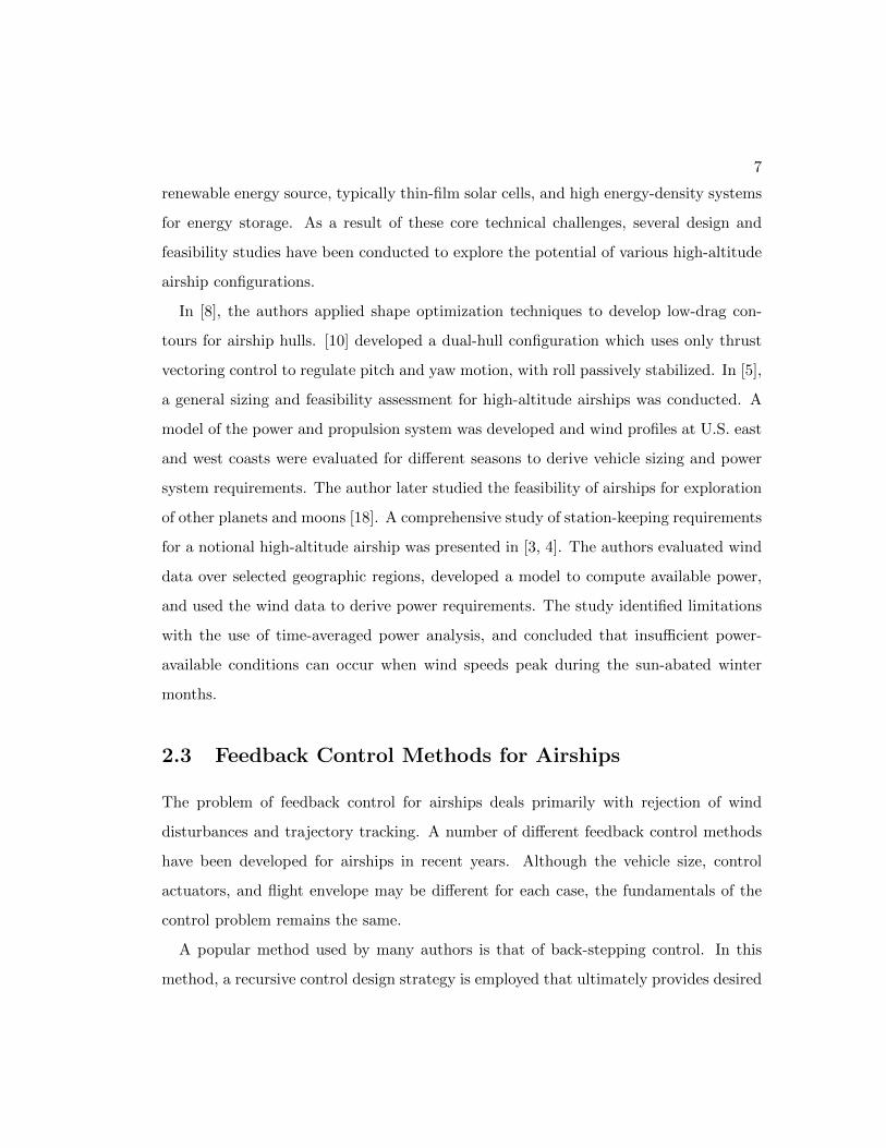
2.3 Feedback Control Methods for Airships
The problem of feedback control for airships deals primarily with rejection of wind
disturbances and trajectory tracking. A number of different feedback control methods
have been developed for airships in recent years. Although the vehicle size, control
actuators, and flight envelope may be different for each case, the fundamentals of the
control problem remains the same.
A popular method used by many authors is that of back-stepping control. In this
method, a recursive control design strategy is employed that ultimately provides desired

8
characteristics to the closed-loop system. [15] developed reduced-order models across
multiple phases of flight and developed feedback control laws with back-stepping meth-
ods. [19] also applied a back-stepping control design, and focused on the airship hover
stabilization problem, using a quaternion formulation for the kinematic equations. In
[11], a back-stepping approach was again used, and global asymptotic stability is shown
with Lyapunov methods.
Several other methods have also been used. In [14], a simple proportional feedback
law was used to control speed, altitude and ground-track errors, and a rapidly exploring
random tree method is used to verify algorithm performance subject to bounded wind
disturbances. [20] presented a study of dynamic inversion, back-stepping, and sliding
mode control techniques applied to global non-linear control of autonomous airships.
[12] generated dynamically feasible trajectories for airships in which preliminary 3D
trajectories for the point mass were created, and open-loop controls required to track
the trajectory were then derived from the dynamic constraints. [4] used loop-shaping
methods to develop inner and outer loop control laws for a notional high-altitude airship
configuration. A detailed investigation of turbulence and wind-gust effects on control
performance was performed, which found a significant increase in the control power.
2.4 Trajectory Planning Methods for Airships
Although numerous feedback control methods for airships are found in the literature,
relatively few studies have been conducted for airship trajectory optimization.
Ref. [21] generates paths of minimum distance that follow a prescribed set of way-
points, subject to kinematic constraints, and Ref. [22] computes helices as candidate
paths for ascent that maintain trim conditions. However, neither of these studies ac-
count for the wind. In Ref. [23], minimum energy and minimum time trajectories are
computed using a wind model of stacked homogeneous layers. This approach ignores
the dynamics of the vehicle, assuming only vertical control is used to enable the airship

9
to traverse between wind layers, with horizontal motion governed completely by the
wind.
In Ref. [16], optimal control problems were formulated for selected scenarios using
a three degree-of-freedom (DOF) point mass model [24], and numerical solutions were
developed to find optimal trajectories in the presence of horizontal winds. While repre-
senting the first work of this type, this initial study was limited in scope to high-altitude
station transitions and station-keeping. In a recent paper [2], optimal ascent trajecto-
ries were designed for the Korean stratospheric airship, with both minimum-time and
minimum-energy solutions, and the enforcement of a convex horizontal excursion con-
straint to keep the flight path within national borders. It is one of the few comprehensive
publications of a stratospheric airship model, incorporating wind-tunnel test data, CFD
analysis, and prototype flight data. However, it also has some important restrictions;
namely, it does not consider the possibility of open initial or final positions, and it de-
fines a performance index for the minimum-energy case that does not reflect the true
energy consumption of the vehicle.

Chapter 3
Modeling
3.1 Fundamentals of Airship Operation
While the airship does share many common attributes with traditional aircraft, sev-
eral properties are fundamentally different. The unique properties of airships must be
understood in order to develop meaningful models and problem formulations.
The buoyancy force acting on the airship is equivalent to the weight of displaced air,
so
B = UHρ(h)g
where UH is the entire volume of the airship, and ρ(h) is the altitude-dependent atmo-
spheric density. The weight of the airship is
W = [m0 +ma(h)]g
where m0 includes the mass of the solid airship structure, payload and Helium, while
ma(h) represents the changing mass of air inside the ballonets.
In order to achieve static buoyancy, or zero net lift, the air mass inside the airship
must change with altitude according to:
ma(h) = UHρa(h)−m0 (3.1)
10

11
The ceiling altitude, or pressure altitude, occurs when the ballonets fully deflate, at
which ma(h) = 0, or
ρa(h) = m0/UH
The rate at which air enters or leaves the ballonets is constrained by the capabilities
of the fans in the pressure regulation system. This translates into imposed limits on the
rate of ascent or descent, in order to maintain neutral buoyancy. I make the assumption
that neutral buoyancy is maintained throughout the flight. This is standard practice
for pressurized airship configurations, which were briefly introduced in Section 1.1. By
maintaining neutral buoyancy, the airship can hover at any altitude, with the capability
to change altitude through forward flight. The pressure regulation system expels air
from the ballonets during ascent to become lighter with the lightening air. Similarly,
it draws air into the ballonets during descent to become heavier. Thus, the maximum
attainable rate of climb with neutral buoyancy depends upon the achievable volume
flow rate of the pressure system.
In addition, the required thrust and power change with flight condition, according
to:
Treq = D =1
2ρ(h)V 2U
2/3H CDo (3.2)
Preq =TreqV
η(3.3)
where q = 12ρ(h)V 2 is the dynamic pressure, Sref = U
2/3H is the standard aerodynamic
reference area for airships, and η is the combined efficiency of the propeller and motor.
3.2 Baseline Design
The baseline airship design used for all subsequent analysis is a semi-rigid configuration
with a pressurized hull and additional structure for housing the payload and onboard
systems, which include avionics, propulsion, power generation, and energy storage. In
these configurations, the pressure regulation system causes the vehicle density to closely
12
match the ambient density, so that the net static lift is nearly zero. In other words, the
buoyancy force closely matches the weight throughout the flight envelope.
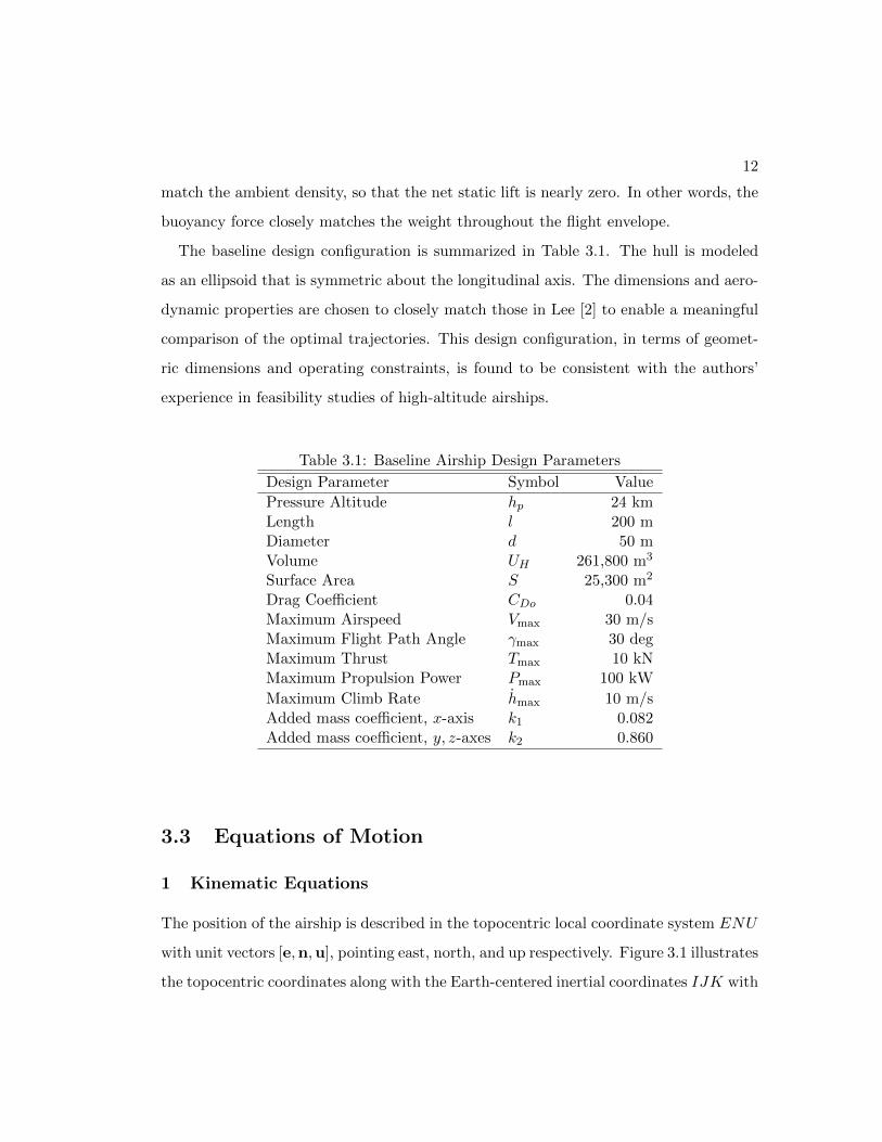
The baseline design configuration is summarized in Table 3.1. The hull is modeled
as an ellipsoid that is symmetric about the longitudinal axis. The dimensions and aero-
dynamic properties are chosen to closely match those in Lee [2] to enable a meaningful
comparison of the optimal trajectories. This design configuration, in terms of geomet-
ric dimensions and operating constraints, is found to be consistent with the authors’
experience in feasibility studies of high-altitude airships.
Table 3.1: Baseline Airship Design Parameters
Design Parameter Symbol Value
Pressure Altitude hp 24 kmLength l 200 mDiameter d 50 mVolume UH 261,800 m3
Surface Area S 25,300 m2
Drag Coefficient CDo 0.04Maximum Airspeed Vmax 30 m/sMaximum Flight Path Angle γmax 30 degMaximum Thrust Tmax 10 kNMaximum Propulsion Power Pmax 100 kW
Maximum Climb Rate hmax 10 m/sAdded mass coefficient, x-axis k1 0.082Added mass coefficient, y, z-axes k2 0.860
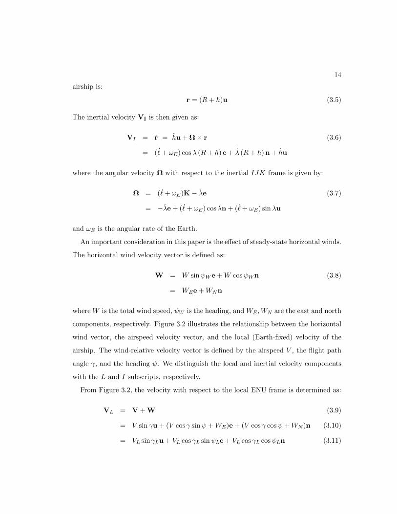
3.3 Equations of Motion
1 Kinematic Equations
The position of the airship is described in the topocentric local coordinate system ENU
with unit vectors [e,n,u], pointing east, north, and up respectively. Figure 3.1 illustrates
the topocentric coordinates along with the Earth-centered inertial coordinates IJK with

13
unit vectors [I,J,K]. Note that ` is the Earth-relative longitude, and the Earth rotates
around the K vector at the rate of ωE . Here, λ is the latitude, ` is the longitude, R is
the Earth radius, and h is the airship altitude, exaggerated for clarity.
I
J
i
K
n e
hR
u
ℓ + ω t
λ
E
Figure 3.1: Topocentric Coordinate System
Derivation of airship equations involves three velocity concepts: inertial velocity,
Earth-relative or local velocity, and wind-relative velocity. Considering the rotation of
the Earth, the inertial velocity is found by:
VI = VL + E (3.4)
where E = ωE(R + h) cosλe. If the Earth rotation is assumed zero, then E = 0 and
VI = VL, meaning that the local frame becomes the inertial frame. We include the
Earth rotation terms throughout this derivation in order to examine the size of the
resulting acceleration terms. In addition, although the spherical-Earth effects are small
considering the ranges involved in this study, including them in the equations of motion
leads to a general-purpose model suitable for ascent and station-transfer planning over
extremely large distances.
To obtain the inertial velocity, we differentiate the position vector with respect to
the inertial IJK frame and express the result in the ENU frame. The position of the
14
airship is:
r = (R+ h)u (3.5)
The inertial velocity VI is then given as:
VI = r = hu + Ω× r (3.6)
= ( ˙ + ωE) cosλ (R+ h) e + λ (R+ h) n + hu
where the angular velocity Ω with respect to the inertial IJK frame is given by:
Ω = ( ˙ + ωE)K− λe (3.7)
= −λe + ( ˙ + ωE) cosλn + ( ˙ + ωE) sinλu
and ωE is the angular rate of the Earth.
An important consideration in this paper is the effect of steady-state horizontal winds.
The horizontal wind velocity vector is defined as:
W = W sinψWe +W cosψWn (3.8)
= WEe +WNn
where W is the total wind speed, ψW is the heading, and WE ,WN are the east and north
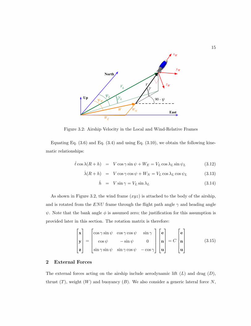
components, respectively. Figure 3.2 illustrates the relationship between the horizontal
wind vector, the airspeed velocity vector, and the local (Earth-fixed) velocity of the
airship. The wind-relative velocity vector is defined by the airspeed V , the flight path
angle γ, and the heading ψ. We distinguish the local and inertial velocity components
with the L and I subscripts, respectively.
From Figure 3.2, the velocity with respect to the local ENU frame is determined as:
VL = V + W (3.9)
= V sin γu + (V cos γ sinψ +WE)e + (V cos γ cosψ +WN )n (3.10)
= VL sin γLu + VL cos γL sinψLe + VL cos γL cosψLn (3.11)
15
zW
WE
WN
ψWγL
VL
ψL90 - ψ
WEast
North
Vγ
Up
xW
yW
Figure 3.2: Airship Velocity in the Local and Wind-Relative Frames
Equating Eq. (3.6) and Eq. (3.4) and using Eq. (3.10), we obtain the following kine-
matic relationships:
˙ cosλ(R+ h) = V cos γ sinψ +WE = VL cosλL sinψL (3.12)
λ(R+ h) = V cos γ cosψ +WN = VL cosλL cosψL (3.13)
h = V sin γ = VL sinλL (3.14)
As shown in Figure 3.2, the wind frame (xyz) is attached to the body of the airship,
and is rotated from the ENU frame through the flight path angle γ and heading angle
ψ. Note that the bank angle φ is assumed zero; the justification for this assumption is
provided later in this section. The rotation matrix is therefore:
x
y
z
=
cos γ sinψ cos γ cosψ sin γ
cosψ − sinψ 0
sin γ sinψ sin γ cosψ − cos γ
e
n
u
= C
e
n
u
(3.15)
2 External Forces
The external forces acting on the airship include aerodynamic lift (L) and drag (D),
thrust (T ), weight (W ) and buoyancy (B). We also consider a generic lateral force N ,
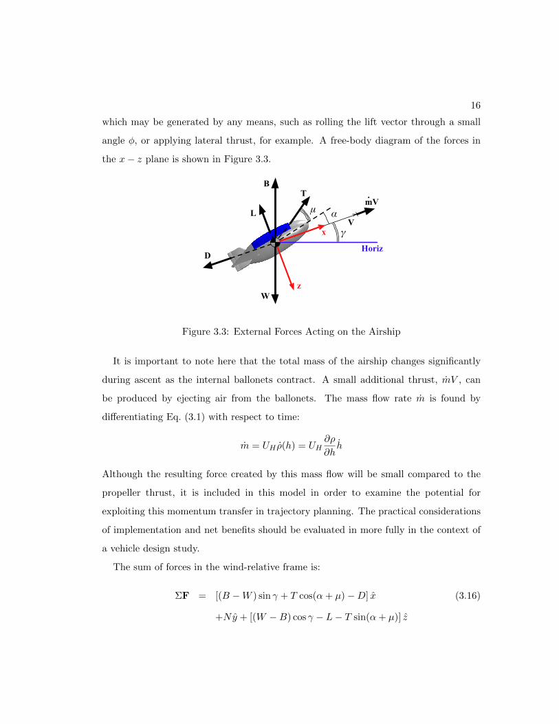
16
which may be generated by any means, such as rolling the lift vector through a small
angle φ, or applying lateral thrust, for example. A free-body diagram of the forces in
the x− z plane is shown in Figure 3.3.
x
μL α
B
W
V
Horiz
z
T
γ
D
mV.
Figure 3.3: External Forces Acting on the Airship
It is important to note here that the total mass of the airship changes significantly
during ascent as the internal ballonets contract. A small additional thrust, mV , can
be produced by ejecting air from the ballonets. The mass flow rate m is found by
differentiating Eq. (3.1) with respect to time:
m = UH ρ(h) = UH∂ρ
∂hh
Although the resulting force created by this mass flow will be small compared to the
propeller thrust, it is included in this model in order to examine the potential for
exploiting this momentum transfer in trajectory planning. The practical considerations
of implementation and net benefits should be evaluated in more fully in the context of
a vehicle design study.
The sum of forces in the wind-relative frame is:
ΣF = [(B −W ) sin γ + T cos(α+ µ)−D] x (3.16)
+Ny + [(W −B) cos γ − L− T sin(α+ µ)] z
17
where the lift and drag forces are defined as L = qU2/3H CL(α) and D = qU
2/3H CD(α),
respectively. The lift and drag coefficients from Lee [2] are used, and are assumed to
vary only with angle of attack.
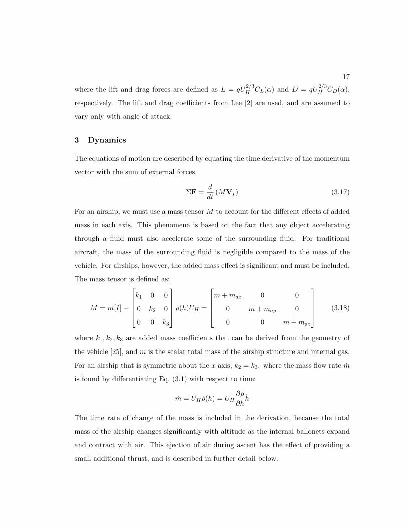
3 Dynamics
The equations of motion are described by equating the time derivative of the momentum
vector with the sum of external forces.
ΣF =d
dt(MVI) (3.17)
For an airship, we must use a mass tensor M to account for the different effects of added
mass in each axis. This phenomena is based on the fact that any object accelerating
through a fluid must also accelerate some of the surrounding fluid. For traditional
aircraft, the mass of the surrounding fluid is negligible compared to the mass of the
vehicle. For airships, however, the added mass effect is significant and must be included.
The mass tensor is defined as:
M = m[I] +
k1 0 0
0 k2 0
0 0 k3
ρ(h)UH =
m+max 0 0
0 m+may 0
0 0 m+maz
(3.18)
where k1, k2, k3 are added mass coefficients that can be derived from the geometry of
the vehicle [25], and m is the scalar total mass of the airship structure and internal gas.
For an airship that is symmetric about the x axis, k2 = k3. where the mass flow rate m
is found by differentiating Eq. (3.1) with respect to time:
m = UH ρ(h) = UH∂ρ
∂hh
The time rate of change of the mass is included in the derivation, because the total
mass of the airship changes significantly with altitude as the internal ballonets expand
and contract with air. This ejection of air during ascent has the effect of providing a
small additional thrust, and is described in further detail below.
18
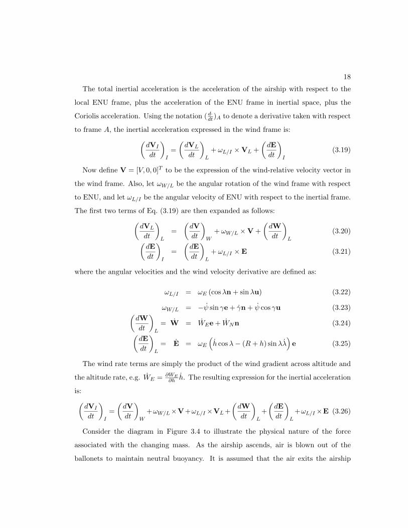
The total inertial acceleration is the acceleration of the airship with respect to the
local ENU frame, plus the acceleration of the ENU frame in inertial space, plus the
Coriolis acceleration. Using the notation ( d·dt)A to denote a derivative taken with respect
to frame A, the inertial acceleration expressed in the wind frame is:
(dVI
dt
)
I
=
(dVL
dt
)
L
+ ωL/I ×VL +
(dE
dt
)
I
(3.19)
Now define V = [V, 0, 0]T to be the expression of the wind-relative velocity vector in
the wind frame. Also, let ωW/L be the angular rotation of the wind frame with respect
to ENU, and let ωL/I be the angular velocity of ENU with respect to the inertial frame.
The first two terms of Eq. (3.19) are then expanded as follows:
(dVL
dt
)
L
=
(dV
dt
)
W
+ ωW/L ×V +
(dW
dt
)
L
(3.20)
(dE
dt
)
I
=
(dE
dt
)
L
+ ωL/I ×E (3.21)
where the angular velocities and the wind velocity derivative are defined as:
ωL/I = ωE (cosλn + sinλu) (3.22)
ωW/L = −ψ sin γe + γn + ψ cos γu (3.23)(dW
dt
)
L
= W = WEe + WNn (3.24)
(dE
dt
)
L
= E = ωE
(h cosλ− (R+ h) sinλλ
)e (3.25)
The wind rate terms are simply the product of the wind gradient across altitude and
the altitude rate, e.g. WE = ∂WE∂h h. The resulting expression for the inertial acceleration
is:
(dVI
dt
)
I
=
(dV
dt
)
W
+ωW/L×V+ωL/I×VL+
(dW
dt
)
L
+
(dE
dt
)
L
+ωL/I×E (3.26)
Consider the diagram in Figure 3.4 to illustrate the physical nature of the force
associated with the changing mass. As the airship ascends, air is blown out of the
ballonets to maintain neutral buoyancy. It is assumed that the air exits the airship

19
at a velocity equal and opposite to the current airspeed, so that it has zero velocity
with respect to the surrounding air. Consider now the change in linear
- dm
z
xV
Horiz
γ
V
m(h) + dm
Air
dV
Figure 3.4: Conservation of Linear Momentum
momentum experienced by the airship over a time interval dt. The original system has
mass m(h) + dm and flies at velocity V + dV . The new system after ejecting the air
has the airship with mass m(h) and velocity V , and the lost mass −dm with velocity
−V relative to the airship. The inertial velocity of the ejected air is V − V = 0. In the
absence of external forces, linear momentum must be conserved. We therefore have:
(m(h) + dm) (V + dV )− dm (V − V ) = m(h)V (3.27)
Neglecting second order differential terms, then dividing by dt and including forces in
the x direction, the above expression leads to:
ΣFx = m(h)dV
dt+ V
dm
dt(3.28)
which is consistent with Eq. (3.17). The effect is similar in principle to the thrust
produced by a rocket, although clearly much smaller in magnitude. Note that the
velocity V here is the airspeed velocity, which is always positive, and the mass flow rate
is always negative during ascent, so that the additional force due to mass flow rate is
always positive in the x direction during ascent.

20
4 Complete Equations of Motion
The complete equations of motion of the airship include the rate of change of its geo-
graphic position, provided in the kinematic Eqs. (3.12) through (3.14), and the rate of
change of its wind-relative velocity. The velocity vector derivative is found by differ-
entiating Eq. (3.4) with respect to the inertial frame, and expressing the result in the
wind frame.
Expanding Eq. (3.26) with Eq. (3.16) and Eq. (3.17), we obtain the following expres-
sions for the time-rate of change of the wind-relative velocity components:
V =(B −W ) sin γ + T cosα−D − UH ρV
m+max− Wx − aEx (3.29)
γ =(B −W ) cos γ + T sinα+ L
(m+maz)V+Wz + aEz
V(3.30)
ψ =N
(m+may)V cos γ− Wy + aEy
V cos γ(3.31)
where the wind rate terms in the wind frame are
Wx = WE cos γ sinψ + WN cos γ cosψ (3.32)
Wy = WE cos γ − WN sin γ (3.33)
Wz = WE sin γ sinψ + WN sin γ cosψ (3.34)
The additional acceleration due to the rotation of the Earth is:
aE =
aEx
aEy
aEz
= ωL/I ×VL +
(dE
dt
)
L
+ ωL/I ×E (3.35)
21
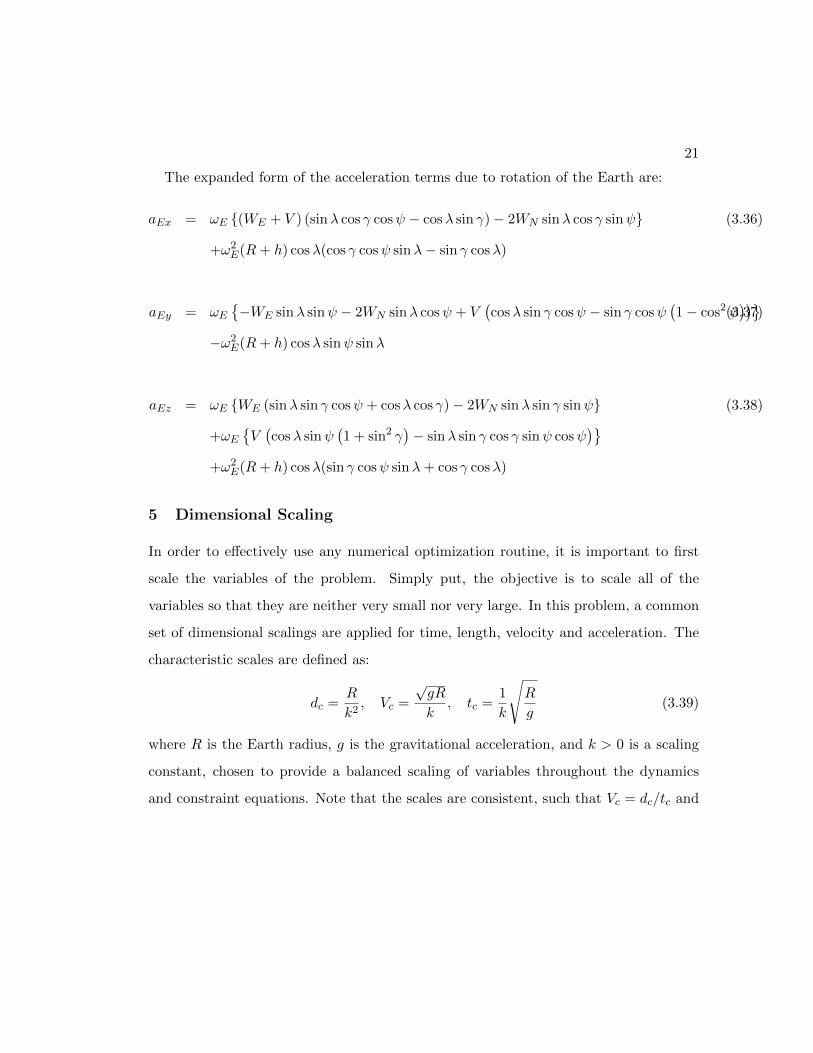
The expanded form of the acceleration terms due to rotation of the Earth are:
aEx = ωE (WE + V ) (sinλ cos γ cosψ − cosλ sin γ)− 2WN sinλ cos γ sinψ (3.36)
+ω2E(R+ h) cosλ(cos γ cosψ sinλ− sin γ cosλ)
aEy = ωE−WE sinλ sinψ − 2WN sinλ cosψ + V
(cosλ sin γ cosψ − sin γ cosψ
(1− cos2 ψ
))(3.37)
−ω2E(R+ h) cosλ sinψ sinλ
aEz = ωE WE (sinλ sin γ cosψ + cosλ cos γ)− 2WN sinλ sin γ sinψ (3.38)
+ωEV(cosλ sinψ
(1 + sin2 γ
)− sinλ sin γ cos γ sinψ cosψ
)
+ω2E(R+ h) cosλ(sin γ cosψ sinλ+ cos γ cosλ)
5 Dimensional Scaling
In order to effectively use any numerical optimization routine, it is important to first
scale the variables of the problem. Simply put, the objective is to scale all of the
variables so that they are neither very small nor very large. In this problem, a common
set of dimensional scalings are applied for time, length, velocity and acceleration. The
characteristic scales are defined as:
dc =R
k2, Vc =
√gR
k, tc =
1
k
√R
g(3.39)
where R is the Earth radius, g is the gravitational acceleration, and k > 0 is a scaling
constant, chosen to provide a balanced scaling of variables throughout the dynamics
and constraint equations. Note that the scales are consistent, such that Vc = dc/tc and
22
g = Vc/tc. The normalized variables are defined as:
V =V
Vc, h =
h
dc, τ =
t
tc(3.40)
WE =WE
Vc, WN =
WN
Vc(3.41)
T =T
UHρ(h0)g, ρ(h) =
ρ(h)
ρ(h0)(3.42)
and the normalized lift and drag forces are expressed as:
L =L
UHρ(h)g= ACL(α)V 2 (3.43)
D =D
UHρ(h)g= ACD(α)V 2 (3.44)
where A = dc/(2U1/3H ). Additionally, the normalized time derivative is related to the
original time derivative as follows:
( )′ =d( )
dτ= tc
d( )
dt= tc ˙( ) ⇒ ( )′ =
1
k
√R
g˙( )
After some algebra, the complete set of equations can now be written in non-dimensional
form as follows:
V ′ =1
1 + k1
T cos(α+ µ)− ∂ρ
∂hsin γV 2
ρ(h)−ACD(α)V 2
− ∂Wx
∂hV sin γ − aEx(3.45)
γ′ =1
1 + k2
T sin(α+ µ)
ρ(h)V+ACL(α)V
+∂Wz
∂hsin γ + aEz/V (3.46)
`′ =V cos γ sinψ + WE
cosλ(R+ h)(3.47)
λ′ =V cos γ cosψ + WN
(R+ h)(3.48)
h′ = V sin γ (3.49)
6 Assumptions
We first discuss the omission of bank angle in these equations. Traditional aircraft
turn by banking, which rotates the lift vector to create lateral acceleration. However,

23
this form of turning is not necessarily the best option for airships, for at least three
reasons. First, airships produce much less dynamic lift than traditional aircraft, as air-
ships rely primarily on buoyancy for the lifting force. Second, the combination of the
weight and buoyancy forces creates a natural stabilizing moment about the roll axis, as
the center of buoyancy is located above the center of gravity. This stabilizing moment
must be overcome in order to hold a non-zero bank angle over time. To perform this
maneuver aerodynamically would require large control surfaces, which, for the strato-
spheric airship, would bring a significant increase weight and drag. Third, the types of
payloads for station-keeping missions will likely be Earth-pointing or zenith pointing.
Large bank angles would tend to violate these payload pointing requirements for fixed
mounted payloads, whereas pure yaw maneuvers would pose no problem. It is therefore
reasonable to consider other mechanisms for turning that do not rely on bank angle,
such as differential thrust to turn with sideslip, or pure lateral thrust. The inherent roll
limitation is evidenced in [2], where bank angle is used as a control input, but with a
limit of only 5 deg. As a consequence of these practical airship design constraints, we
assume bank angle remains sufficiently close to zero such that it can be ignored in the
equations of motion.
In this paper, we assume that the airship regulates internal pressure to maintain zero
static lift (B = W ) throughout the flight envelope. The longitudinal control inputs
are angle-of-attack α, thrust T , and thrust vector angle µ. We choose the lateral con-
trol input to be heading ψ, and enforce bounds on ψ. The states of the system are the
wind-relative velocity V , flight path angle γ, and the geographic position [`, λ, h]. There-
fore, the state equations for the system include the kinematic expressions, Eqs. (3.12)
through Eqs. (3.14), and the longitudinal velocity derivatives, Eqs. (3.29) and (3.30).
To summarize, this formulation of the airship equations of motion includes the point
mass kinematic equations for a spherical Earth, steady-state horizontal winds that vary
with altitude, longitudinal dynamics governed by lift, drag and vectored thrust, mass
variation with altitude, the effects of added mass, and virtual accelerations due to wind
24
variations and Earth rotation. This formulation is more general than the model provided
in Lee [2], in that it includes Earth rotation and mass variation across altitude. Also
note that the dynamic relationship of ψ with the other states and controls, given in
Eq. (3.31), can be used as a time varying constraint if desired. However, for this study
we impose constant bounds on ψ.
3.4 Environment Models
The stratospheric airship must fly through a wide range of flight conditions, from 0 to
30 m/s airspeed, and from sea-level to about 21 km altitude. Across this altitude
range, the atmospheric density and steady-state wind velocity change considerably. The
subsections below describe the models used to approximate the atmospheric density and
wind across altitude. A model of the solar power generated during flight is provided in
Section 3.5.
1 Atmospheric Density
During its ascent, the atmospheric density drops by a factor of 16, from 1.225 to about
0.075 kg/m3. I assume the atmospheric density changes with altitude according to
the standard atmosphere model [26]. A third order polynomial is fit to the standard
atmosphere data over an altitude range of 0 to 23 km. The altitude is normalized prior
to fitting to obtain better numerical accuracy. The polynomial expression is given as:
ρ(h) = ρ(0)[c0 + c1(h/dc) + c2(h/dc)
2 + c3(h/dc)3]
(3.50)
where dc is a dimensional scaling parameter, defined in Eq. (3.39). Using dc = 15, 891.915 km
and c = [−0.11159, 0.71537, −1.45854, 0.99523]T gives a maximum error of 2.6% and a
mean error of 0.84%.
25
2 Horizontal Wind Model
The average wind velocity also changes considerably with altitude, although with much
less predictability than that of the density variation. The general trend is that windspeed
gradually increases during ascent through the troposphere, reaching a peak in the jet-
stream altitude range of 10-15 km. It then gradually decreases again to reach a minimum
speed in the lower portion of the stratosphere, generally between 18-25 km. The actual
wind profile changes with geographic location and the time of year, and is also effected
by the 11-year solar cycle.
In general, wind velocity can be split into steady-state and time-varying components.
While the actual winds encountered during flight cannot be predicted exactly, steady-
state horizontal winds are known to follow specific trends with altitude, geographic
position, and the time of year. Typical wind behavior can be adequately characterized
based upon meteorological data, which provides a mechanism for design-phase planning.
In addition, weather balloons and other instruments can be used immediately prior to
flight, for pre-flight and onboard planning.
The 1993 horizontal wind model (HWM93), produced by the Naval Research Labora-
tory (NRL), uses a combination of historical meteorological data and measurements from
radar and rocket sounding experiments to develop an analytic emperical model [27]. A
FORTRAN program of the HWM93, available on the NRL website[28], was used to gen-
erate wind profiles over altitude at select times and geographic locations. In this paper,
we use the HWM93 to model the average wind profile at the coordinates of 118o 0.0′ W,
35o 0.0′ N. This is located at the southern end of Edwards AFB, approximately 100 km
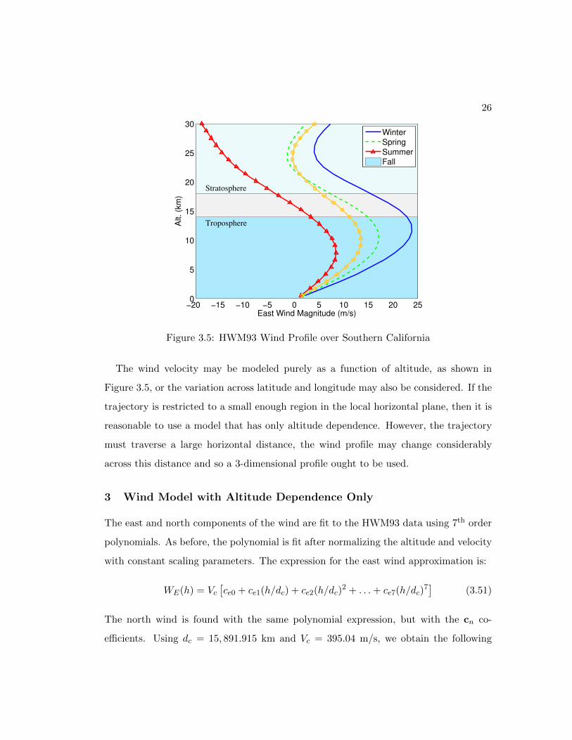
north of Los Angeles. The variation of the east component of wind across altitude is
shown in Figure 3.5 for four different times of year. The north component of the wind is
not shown, as it the maximum speed is under 1 m/s. This is representative of the typi-
cal wind profile observed in the continental U.S., with the peak speeds occurring in the
jet-stream altitude range of 10-15 km, and with the wind directed primarily eastward.
26
−20 −15 −10 −5 0 5 10 15 20 250
5
10
15
20
25
30
East Wind Magnitude (m/s)
Alt. (k
m)
Troposphere
Stratosphere
WinterSpring
SummerFall
Figure 3.5: HWM93 Wind Profile over Southern California
The wind velocity may be modeled purely as a function of altitude, as shown in
Figure 3.5, or the variation across latitude and longitude may also be considered. If the
trajectory is restricted to a small enough region in the local horizontal plane, then it is
reasonable to use a model that has only altitude dependence. However, the trajectory
must traverse a large horizontal distance, the wind profile may change considerably
across this distance and so a 3-dimensional profile ought to be used.
3 Wind Model with Altitude Dependence Only
The east and north components of the wind are fit to the HWM93 data using 7th order
polynomials. As before, the polynomial is fit after normalizing the altitude and velocity
with constant scaling parameters. The expression for the east wind approximation is:
WE(h) = Vc[ce0 + ce1(h/dc) + ce2(h/dc)
2 + . . .+ ce7(h/dc)7]
(3.51)
The north wind is found with the same polynomial expression, but with the cn co-
efficients. Using dc = 15, 891.915 km and Vc = 395.04 m/s, we obtain the following

27
coefficients for the winter season wind model:
ce = [−0.16235, 0.8355, −1.64017, 1.60473, −0.8928, 0.20646, 0.09708, 0.00246]T(3.52)
cn = [−0.00103, 0.0050, −0.00789, 0.00459, −0.0010, −0.00085, 0.00047, −0.00001]T(3.53)
The approximations match the original model with a maximum error of 0.4% in the
east component, and 1.1% in the north component.
3.5 Solar Power Generation Model
One of the fundamental design features of stratospheric airships is that they can use
hull-mounted thin film solar cells to generate sufficient power for sustained flight. Solar
power is converted into electricity, which is used to operate the payload, electric motors
and avionics, and to charge batteries. The process of performing this power manage-
ment is not trivial, and is undoubtedly one of the most challenging design aspects of
these airships. Although the power management system cannot be easily modeled, it is
possible to develop a general model for the total solar power available to the airship.
The available solar power depends upon a variety of factors. This includes factors
beyond our control (the time of year, time of day, and geographic location), vehicle
design factors (the solar cell coverage area and hull geometry), and lastly, operational
factors (airship orientation). This section provides a model for computing the total
solar power that can be captured by the hull-mounted solar cells as a function of hull
geometry, latitude, time, airship orientation, and altitude. A similar model is presented
in Wang et.al. [29], but it provides no way to model the significant variation in received
solar flux across altitude.
It is also important to note that the efficiency of the solar cells in absorbing and
converting solar energy is not included in the model presented here. Thus, solar cell
efficiency may be treated completely independently of this model.
28
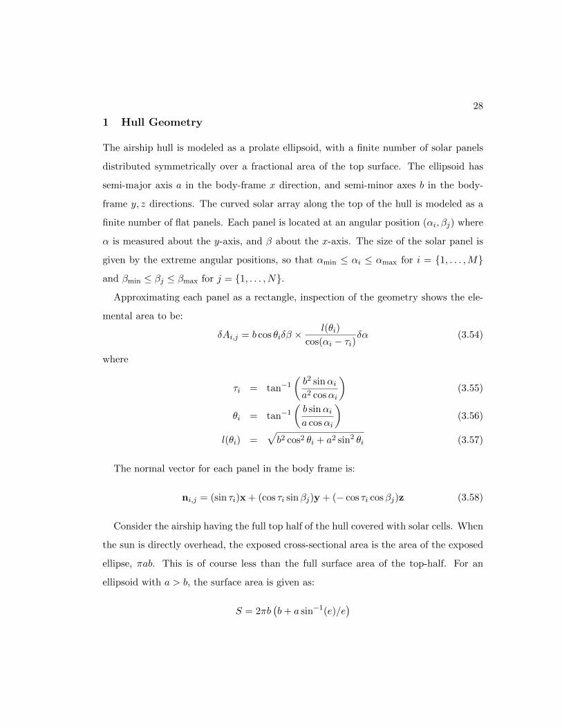
1 Hull Geometry
The airship hull is modeled as a prolate ellipsoid, with a finite number of solar panels
distributed symmetrically over a fractional area of the top surface. The ellipsoid has
semi-major axis a in the body-frame x direction, and semi-minor axes b in the body-
frame y, z directions. The curved solar array along the top of the hull is modeled as a
finite number of flat panels. Each panel is located at an angular position (αi, βj) where
α is measured about the y-axis, and β about the x-axis. The size of the solar panel is
given by the extreme angular positions, so that αmin ≤ αi ≤ αmax for i = 1, . . . ,Mand βmin ≤ βj ≤ βmax for j = 1, . . . , N.
Approximating each panel as a rectangle, inspection of the geometry shows the ele-
mental area to be:
δAi,j = b cos θiδβ ×l(θi)
cos(αi − τi)δα (3.54)
where
τi = tan−1
(b2 sinαia2 cosαi
)(3.55)
θi = tan−1
(b sinαia cosαi
)(3.56)
l(θi) =√b2 cos2 θi + a2 sin2 θi (3.57)
The normal vector for each panel in the body frame is:
ni,j = (sin τi)x + (cos τi sinβj)y + (− cos τi cosβj)z (3.58)
Consider the airship having the full top half of the hull covered with solar cells. When
the sun is directly overhead, the exposed cross-sectional area is the area of the exposed
ellipse, πab. This is of course less than the full surface area of the top-half. For an
ellipsoid with a > b, the surface area is given as:
S = 2πb(b+ a sin−1(e)/e
)

29
where e =√
1− (b/a)2. Dividing the cross-sectional area by the surface area of the top
half, we can determine the total amount of cosine loss due to curvature of the hull. The
total loss simplifies to:
ηC =1
b/a+ sin−1(e)/e(3.59)
This is a particularly useful formula as it is non-dimensional, requiring only the ratio of
semi-minor to semi-major axes, b/a. For the baseline configuration considered in this
paper, b/a = 0.25 and ηC = 0.62. Thus, 38% of the effective solar cell area is lost
immediately due to the curvature of the hull.
2 Sun Vector
The sun vector is defined by its azimuth φs and elevation γs, which change smoothly
with time from dawn to dusk. In the ENU frame, the coordinates of the unit sun vector
are:
s = (cos γs sinφs)e + (cos γs cosφs)n + (sin γs)u (3.60)
The azimuth and elevation can be expressed as follows:
γs = sin−1 (cosh cos d cosλ+ sin d sinλ) (3.61)
φs = sin−1
(−sinh cos d
cos γs
)(3.62)
where h is the local hour angle, starting from 0 at noon and varying through 2π over
24 hours. The sun’s declination d varies with the time of year. In degrees, it can be
expressed as:
d = −23.45 cos
(360
365(td + 10)
)
with 0 ≤ td ≤ 365 representing the time of year in days.
Let C be the rotation matrix that rotates from the ENU frame to the airship body
30
frame. Assuming zero bank angle, C is defined as:
C =
cos γ sinψ cos γ cosψ sin γ
cosψ − sinψ 0
sin γ sinψ sin γ cosψ − cos γ
(3.63)
The sun vector in the body frame is then just Cs.
3 Solar Flux Through All Panels
The total solar flux at any time for the airship is:
F =∑
i,j
Fi,j (3.64)
where Fi,j is the flux at panel (i, j). The solar flux at any time for panel (i, j)) is:
Fi,j = IδAi,j cos ζi,j (3.65)
where I is the local solar irradiance, and ζi,j is the solar incidence angle for panel (i, j).
This is the angle between the normal vector of the panel and the sun vector, which can
be written as:
cos ζi, j = (Cs) · ni,j (3.66)
We must ignore negative fluxes. Therefore, the expression becomes:
Fi,j =
I(h)δAi,j cos ζi,j γs > 0, −π2 ≤ ζi, j ≤ π
2
0 else(3.67)
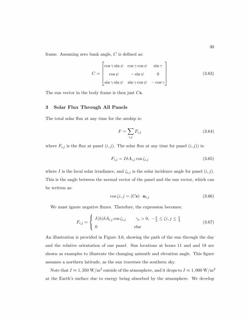
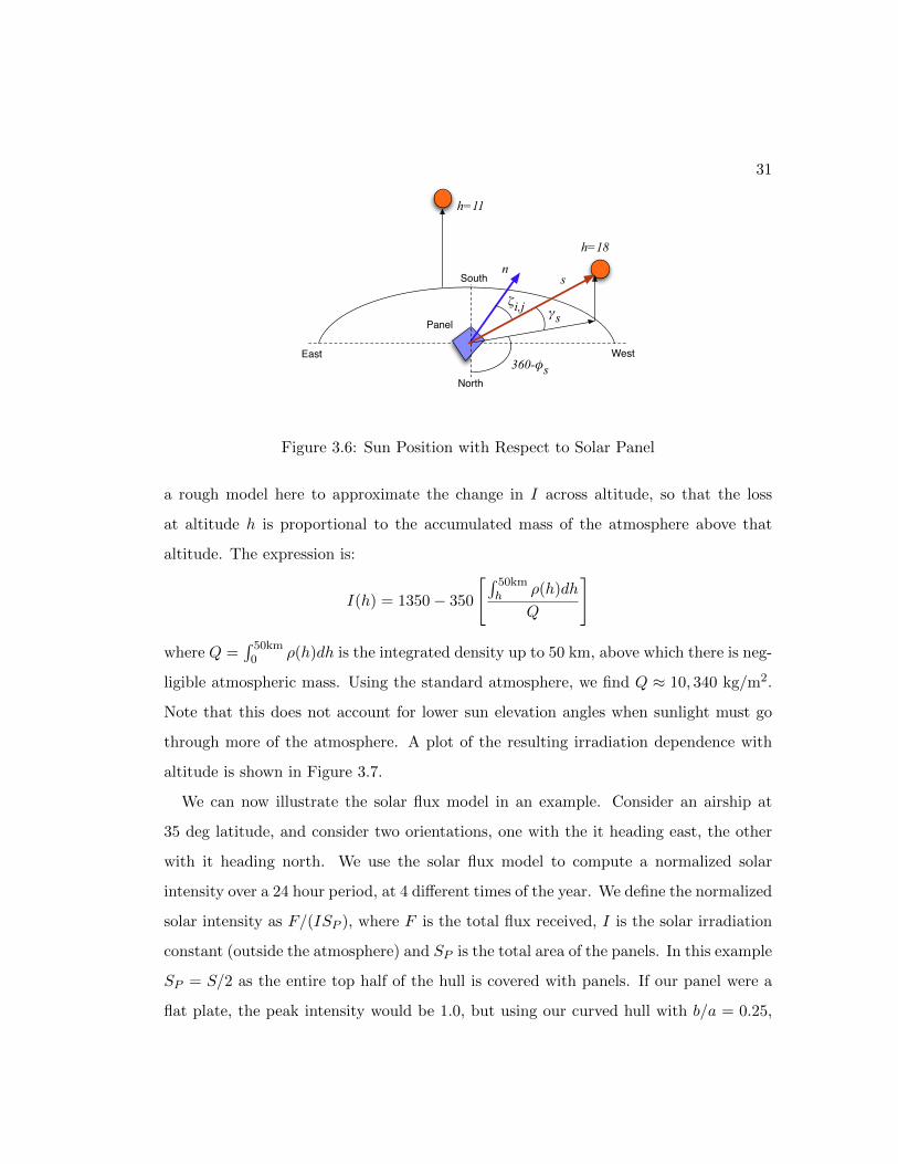
An illustration is provided in Figure 3.6, showing the path of the sun through the day
and the relative orientation of one panel. Sun locations at hours 11 and and 18 are
shown as examples to illustrate the changing azimuth and elevation angle. This figure
assumes a northern latitude, as the sun traverses the southern sky.
Note that I ≈ 1, 350 W/m2 outside of the atmosphere, and it drops to I ≈ 1, 000 W/m2
at the Earth’s surface due to energy being absorbed by the atmosphere. We develop
31
ζi,j
East West
nsSouth
North360-φs
γsPanel
h=11
h=18
Figure 3.6: Sun Position with Respect to Solar Panel
a rough model here to approximate the change in I across altitude, so that the loss
at altitude h is proportional to the accumulated mass of the atmosphere above that
altitude. The expression is:
I(h) = 1350− 350
[∫ 50kmh ρ(h)dh
Q
]
where Q =∫ 50km
0 ρ(h)dh is the integrated density up to 50 km, above which there is neg-
ligible atmospheric mass. Using the standard atmosphere, we find Q ≈ 10, 340 kg/m2.
Note that this does not account for lower sun elevation angles when sunlight must go
through more of the atmosphere. A plot of the resulting irradiation dependence with
altitude is shown in Figure 3.7.
We can now illustrate the solar flux model in an example. Consider an airship at
35 deg latitude, and consider two orientations, one with the it heading east, the other
with it heading north. We use the solar flux model to compute a normalized solar
intensity over a 24 hour period, at 4 different times of the year. We define the normalized
solar intensity as F/(ISP ), where F is the total flux received, I is the solar irradiation
constant (outside the atmosphere) and SP is the total area of the panels. In this example
SP = S/2 as the entire top half of the hull is covered with panels. If our panel were a
flat plate, the peak intensity would be 1.0, but using our curved hull with b/a = 0.25,

32
1000 1050 1100 1150 1200 1250 1300 13500
5
10
15
20
25
30
35
40
45
50
Solar Irradiance (W/m2)
Alti
tude
(km
)
Figure 3.7: Irradiance Variation with Altitude
the peak intensity is 0.62 (see Eq. (3.59). The results of the sample analysis are shown
in Figure 3.8.
Figure 3.8: Normalized Solar Intensity for East-West and North-South Orientations atWinter, Spring/Fall, Summer, for 0 Deg and 30 Deg Pitch Angles
0 5 10 15 20 250
0.1
0.2
0.3
0.4
0.5
0.6
0.7Pitch = 0 deg
Hour of Day
Nor
mal
ized
Sol
ar In
tens
ity
EW WinterEW Spring/FallEW SummerNS WinterNS Spring/FallNS Summer
0 5 10 15 20 250
0.1
0.2
0.3
0.4
0.5
0.6
0.7Pitch = 30 deg
Hour of Day
Nor
mal
ized
Sol
ar In
tens
ity
EW WinterEW Spring/FallEW SummerNS WinterNS Spring/FallNS Summer
For both plots, we see the intensity jumping up at the dawn hour and jumping back
to zero at dusk, the times of which depend on the season. Consider the 0 deg pitch
case first. Here, the plots are symmetric about the noon hour, as we would expect. In

33
every season, the north-south (NS) orientation starts and finishes the day with a larger
intensity than that of the east-west (EW). This is because with a NS orientation, the
long side of the vehicle (with a larger area) is exposed to the sun at these times of the
day. For the summer time, the peak intensity of 0.62 is nearly achieved, as the sun
elevation reaches about 80 deg at this latitude. For the winter time, the intensity does
not climb much during the day as the sun elevation only reaches about 31.5 deg at noon.
Now consider the 30 deg pitch case. Here, the intensity is asymmetric about the
noon hour for the east-west orientations. This is due to the positive pitch angle, which
obstructs the top half of the hull from view of the sun in the morning. This clearly
illustrates the potential for the airship attitude to have a significant impact on its
power generation capability.
4 Remarks
Analyzing the separate contributions of this model, we see that the total solar flux on
the airship depends upon several different factors:
1. The geographic latitude and altitude
2. The time of year and time of day
3. The size and shape of the airship hull
4. The placement of solar cells on the hull surface
5. The orientation of the airship hull
The latitude and altitude are dictated by the mission or application. For long endurance
missions, the time of year will impact the solar flux to greater degrees at larger latitudes.
The size and shape of the hull, and the choice of where to place solar cells, are design
decisions that should be explored in order to best accommodate the expected conditions
for the mission. For example, if it is expected that the majority of the airship’s flight

34
in the northern hemisphere would involve station-keeping against a westerly wind, then
solar panel placement should be biased towards the southern side of the hull to maximize
energy production. The final influence is the orientation of the airship hull with respect
to the sun. The solar flux model may be included in the trajectory optimization phase
in order to develop flight plans that provide improved energy production.
It is also interesting to consider the tradeoff associated with choosing the solar cell
coverage for the vehicle. In some cases, it may be known that a particular orientation
will be flown a majority of the time, due to a high confidence that the wind direction
stays within a certain small range. Under such conditions, the solar cell coverage may
be greatly biased to one side of the vehicle. Otherwise, the coverage may need to be
symmetric to ensure a sufficient solar cell area is available for any possible orientation.
In either case, the question remains as to how much of the hull should be covered in
solar cells. Adding a solar cell adds cost and mass, both for the cell itself and the wiring
to connect it. Clearly it is not desirable to add a cell if it will not receive sufficient
solar power. Combining the solar generation model presented here with a historical,
statistical wind model, one could develop a Monte Carlo simulation to study the energy
production associated with different candidates of solar cell coverage geometries.
Chapter 4
Problem Formulations
We now consider the formulation of trajectory optimization problems for various types
of airship flights. Let the state vector x(t) and control vector u(t) be defined as:
x(t) = [V, γ, `, λ, h]T (4.1)
u(t) = [T, α, µ, ψ]T (4.2)
The airship dynamic model is described by the system of nonlinear differential equations
given in Eqs. (3.12)-(3.14) and Eqs. (3.29)-(3.30), which can be expressed as:
x(t) = f (x(t),u(t), t) (4.3)
The optimization problem is to choose a control history u(t) that minimizes a scalar
performance index, J , subject to the equations of motion over some time interval [t0, tf ],
and other constraints that may be enforced on the states and controls. Specifically, we
enforce constant bounds on the states, controls, and control rates, and impose both path
35
36
constraints χ and terminal constraints Ψ on the state. The problem is summarized as:
minu(t),tf
J(x(t),u(t), t) (4.4)
Subject to x(t) = f (x(t),u(t), t) , x(t0) ∈ X0
xL ≤ x(t) ≤ xU , t > t0
uL ≤ u(t) ≤ uU
uL ≤ u(t) ≤ uU
χ(x(t)) ≤ 0
Ψ(x(tf )) = 0
where X0 represents an allowable set of initial states. The path constraints include
bounds on the climb rate and power, as given below:
χ1 = V sin γ − hmax ≤ 0 (4.5)
χ2 = TV − Pmaxη ≤ 0 (4.6)
The terminal constraint enforces a final desired position (`f , λf , hf ) and speed (VLf ) to
be achieved.
Ψ1 = `(tf )− `f = 0 (4.7)
Ψ2 = λ(tf )− λf = 0 (4.8)
Ψ3 = h(tf )− hf = 0 (4.9)
Ψ4 = (V cos γ cosψ +WN )2 + (V cos γ sinψ +WE)2 − V 2Lf = 0 (4.10)
Two fundamentally different types of optimal ascent trajectories are considered: min-
imum time and minimum energy. Within the context of feedback control design, the
term “energy” is indeed often referred to as the total control effort,∫u2(t)dt. However,
this is not necessarily meaningful for airship trajectory planning, as it does not reflect
the true energy expenditure of the airship during flight. The total energy consumption

37
of the airship during the trajectory is the integral of the required power:
E =
∫ tf
t0
V T
ηdt (4.11)
I consider only the power required for propulsion, ignoring any power required for
payload and/or systems operation, as these are expected to be small in comparison and
are not affected by the trajectory. It is reasonable to assume the efficiency remains
constant throughout the flight, allowing it to be disregarded in the performance index.
We can now define the performance index as
J = Kttf +Kp
∫ tf
t0
V Tdt (4.12)
where Kt and Kp are non-negative weighting coefficients that enable the problem to be
cast as pure minimum time (Kt = 1,Kp = 0), pure minimum energy, (Kt = 0,Kp = 1),
or a blend of both objectives (Kt > 0,Kp > 0).
It is important to note that a more comprehensive model of the airship flight power
requirement would include the power required to operate the pressure regulation system,
which must blow air out of the ballonets during ascent. Providing a more accurate
power model would help to design more realistic trajectories for the minimum energy
problem. In addition, it may be worthwhile to model the maximum air flow rate as a
constraint. This would allow the buoyancy and weight to be modeled separately, with
mass as a state, so that neutral buoyancy conditions are only achieved when the pressure
regulation system can expel or intake air fast enough.

Chapter 5
Numerical Solution Methods
The optimal control problem described above can only be solved numerically. An effec-
tive method for developing a numerical solution is to transform this dynamic optimiz-
ation problem into a parameter optimization problem. We use a collocation approach,
discretizing the dynamic equations so that both the states and controls become decision
variables over a finite number of nodes [30, 31, 32]. We then solve the problem nu-
merically using SNOPT, which is a sequential quadratic programming (SQP) tool that
exploits the sparsity structure of the Jacobian matrix [33].
Define the time interval t ∈ [t0, tf ] over N nodes, so that tk = t0 + τktf , where:
0 = τ1 < τ2 < τ3 < . . . τN−1 < τN = 1
The state and control vectors at time tk are now defined as xk ∈ RNS and uk ∈ RNC ,
respectively. The vector of decision variables is composed of the states and controls over
all nodes, as well as the final time tf , so that X ∈ RND with ND = N(NS +NC) + 1.
X =[xT1 ,x
T1 ,u
T2 ,u
T2 , . . .x
TN ,u
TN , tf
](5.1)
We can now use Simpson’s rule to integrate the dynamic equations. The original dy-
namic constraint is: x(t) = f(x(t),u(t), t). Applying Simpson’s rule to the discrete
38
39
system, we have:
xk ≈xk+1 − xk
∆tk=
1
6[fk + 4fmk + fk+1] (5.2)
where
fk = f(xk,uk) (5.3)
fmk = f(xmk,umk) (5.4)
xmk =1
2(xk + xk+1)− 1
8(fk+1 − fk)∆tk (5.5)
umk =1
2(uk + uk+1) (5.6)
∆tk = (τk+1 − τk)tf (5.7)
These equations of motion provide a set of nonlinear constraint equations, Cf (X) = 0.
Rearranging Eq. (5.2), the kth set of equations are given as:
Cf ,k = xk+1 − xk −1
6[fk + 4fmk + fk+1] ∆tk = 0, k ∈ [1, N − 1] (5.8)
The performance index, originally defined in Eq. (4.12), is now equivalently defined
as:
J(X) = Kttf +Kp
N−1∑
k=1
TkVk (5.9)
The parameter optimization problem is to choose a decision vector X that minimizes
the above performance index, subject to a set of nonlinear constraints of the form
l ≤ C(X) ≤ u, where l and u are fixed lower and upper bounds, respectively. The
full set of constraints includes the equations of motion, the control rate limits, path
constraints on climb rate and power, and the terminal constraints (Ct). The problem
40
can now be stated as:
minX
J(X) (5.10)
Subject to fL ≤ Cf (X) ≤ fU
cL ≤ Cc(X) ≤ cU
pL ≤ Cp(X) ≤ pU
tL ≤ Ct(X) ≤ tU
XL ≤ X ≤ XU
where XL and XU are the lower and upper bounds on the decision variables across all
nodes, Cc ∈ R(N−1)NC is the set of rate limits on NC controls, Cp ∈ RNNP is the set of
NP path constraints over N nodes, and Ct ∈ RNT is the set of NT terminal constraints.
Here, NP = 2 for path constraints on climb rate and power, and NT = 4 for terminal
constraints on latitude, longitude, altitude, and inertial airspeed. The bounds on the
initial state are included in XL,XU .
The kth set of dynamic constraints are given in Eq. (5.8). Because these are equality
constraints, we have fL = fU = 0. The kth set of control rate bounds, expressed as
cL,k ≤ Cc,k ≤ cU,k, are given as:
Tmin
αmin
µmin
ψmin
≤
(Tk+1 − Tk)/∆tk(αk+1 − αk)/∆tk(µk+1 − µk)/∆tk(ψk+1 − ψk)/∆tk
≤
Tmax
αmax
µmax
ψmax
, k ∈ [1, N − 1] (5.11)
The kth set of path constraints are taken from Eq. (4.5) and Eq. (4.6), so that pL,k ≤Cp,k ≤ pU,k is equivalent to:
hmin
0
≤
Vk sin γk
TkVk
≤
hmax
Pmax
, k ∈ [1, N ] (5.12)
Finally, the terminal constraints are taken from Eq. (4.7) through Eq. (4.10). As with
the dynamics, these are enforced as equality constraints, so tL = tU = 0.
41
For numerical solutions, we discretize the problem over 60 nodes and use SNOPT to
compute optimal trajectories for various sets of initial conditions and cost functions.
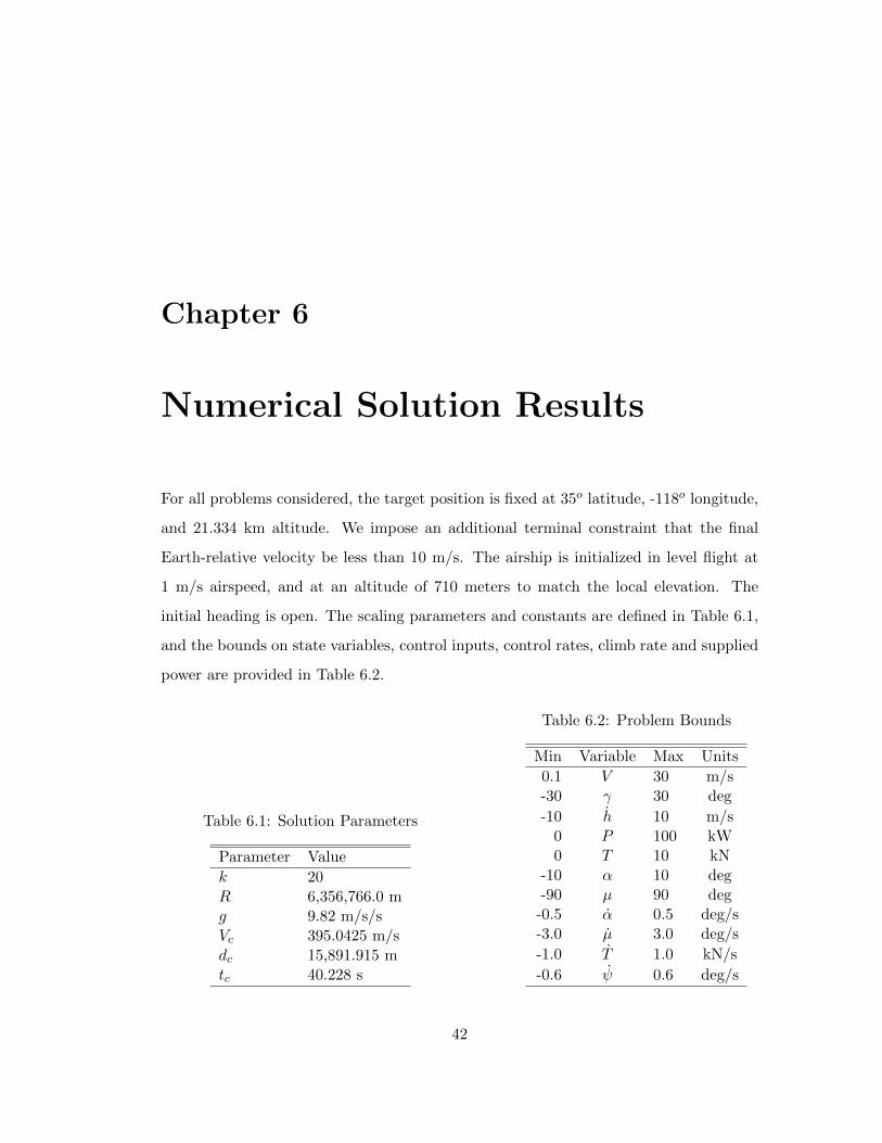
Chapter 6
Numerical Solution Results
For all problems considered, the target position is fixed at 35o latitude, -118o longitude,
and 21.334 km altitude. We impose an additional terminal constraint that the final
Earth-relative velocity be less than 10 m/s. The airship is initialized in level flight at
1 m/s airspeed, and at an altitude of 710 meters to match the local elevation. The
initial heading is open. The scaling parameters and constants are defined in Table 6.1,
and the bounds on state variables, control inputs, control rates, climb rate and supplied
power are provided in Table 6.2.
Table 6.1: Solution Parameters
Parameter Value
k 20R 6,356,766.0 mg 9.82 m/s/sVc 395.0425 m/sdc 15,891.915 mtc 40.228 s
Table 6.2: Problem Bounds
Min Variable Max Units
0.1 V 30 m/s-30 γ 30 deg
-10 h 10 m/s0 P 100 kW0 T 10 kN
-10 α 10 deg-90 µ 90 deg-0.5 α 0.5 deg/s-3.0 µ 3.0 deg/s
-1.0 T 1.0 kN/s
-0.6 ψ 0.6 deg/s
42
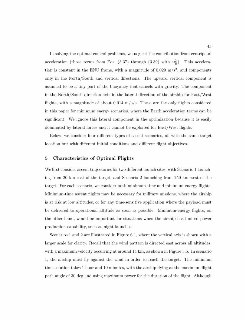
43
In solving the optimal control problems, we neglect the contribution from centripetal
acceleration (those terms from Eqs. (3.37) through (3.39) with ω2E). This accelera-
tion is constant in the ENU frame, with a magnitude of 0.029 m/s2, and components
only in the North/South and vertical directions. The upward vertical component is
assumed to be a tiny part of the buoyancy that cancels with gravity. The component
in the North/South direction acts in the lateral direction of the airship for East/West
flights, with a magnitude of about 0.014 m/s/s. These are the only flights considered
in this paper for minimum energy scenarios, where the Earth acceleration terms can be
significant. We ignore this lateral component in the optimization because it is easily
dominated by lateral forces and it cannot be exploited for East/West flights.
Below, we consider four different types of ascent scenarios, all with the same target
location but with different initial conditions and different flight objectives.
5 Characteristics of Optimal Flights
We first consider ascent trajectories for two different launch sites, with Scenario 1 launch-
ing from 20 km east of the target, and Scenario 2 launching from 250 km west of the
target. For each scenario, we consider both minimum-time and minimum-energy flights.
Minimum-time ascent flights may be necessary for military missions, where the airship
is at risk at low altitudes, or for any time-sensitive application where the payload must
be delivered to operational altitude as soon as possible. Minimum-energy flights, on
the other hand, would be important for situations when the airship has limited power
production capability, such as night launches.
Scenarios 1 and 2 are illustrated in Figure 6.1, where the vertical axis is shown with a
larger scale for clarity. Recall that the wind pattern is directed east across all altitudes,
with a maximum velocity occurring at around 14 km, as shown in Figure 3.5. In scenario
1, the airship must fly against the wind in order to reach the target. The minimum
time solution takes 1 hour and 10 minutes, with the airship flying at the maximum flight
path angle of 30 deg and using maximum power for the duration of the flight. Although

44
−250 −200 −150 −100 −50 0 50 1000
5
10
15
20
25
30
East (km)
Alt
(km
)
Scenario 1
MinTime
MinEnergy
Min Time
Min Energy
Scenario 2
Target
Figure 6.1: Scenarios 1 & 2, Minimum Time and Fixed-Time / Minimum Energy Tra-jectories
the wind blows the airship further east of its launch point, the airship wind-relative
heading is aligned west at all times. This can be seen in the ascent path of the Scenario
1 minimum-time solution in Figure 6.2, which shows the orientation of the airship at
points along the trajectory.
Figure 6.2: Scenario 1 Minimum-Time Ascent Path
In scenario 2, the airship launches much further away at 250 km, but is able to
fly with the wind for the entire flight. The minimum time trajectory takes 2 hours.
The airship first saturates thrust at 10 kN, then immediately reaches the maximum
flight path angle of 30 deg. It continues to accelerate and reaches the power limit of

45
100 kW after 12 minutes. It then cruises at the jet stream altitude of 14 km for about
45 minutes, covering a range of 120 km, and finally climbs to the target station. The
control history for this minimum time case of Scenario 2 is shown in Figure 6.3, and time
histories for velocity, flight path angle, climb rate and power are shown in Figure 6.4.
The Earth-relative heading, flight path angle and velocity are shown as dashed lines.
It is interesting to observe the use of angle of attack as a control. In this and in all
other simulations, the angle of attack is set to -0.78 deg for almost the entire trajectory,
which is the minimum drag angle for the polynomial approximation of drag coefficient
used from [2]. Longitudinal control is achieved primarily by throttling thrust and rotat-
ing the thrust vector through µ. Aerodynamic lift and drag are used sparingly. In this
case, angle of attack control is used only at the end of the trajectory to reduce speed,
so that the final Earth-relative velocity constraint of < 10 m/s can be met.
0
5
10
Thr
ust [
kN]
−10
0
10
α [d
eg]
−50
0
50
µ [d
eg]
0 0.5 1 1.5 2−200
0
200
ψ [d
eg]
Time [hrs]
Wind−RelativeEarth−Relative
Figure 6.3: Scenario 2, Control History for Minimum Time Solution
For the minimum energy flight of scenario 2, the control histories are plotted in
Figure 6.5 and additional time histories are given in Figure 6.6. The trajectory begins
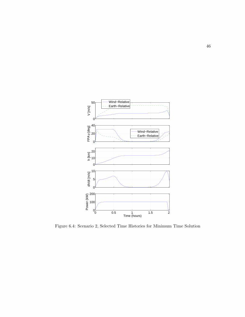
46
0
50
V [m
/s]
Wind−RelativeEarth−Relative
0
20
40
FP
A γ
[deg
]
Wind−RelativeEarth−Relative
0
10
20
h [k
m]
0
5
10
dh/d
t [m
/s]
0 0.5 1 1.5 20
100
200
Pow
er (
kW)
Time (hours)
Figure 6.4: Scenario 2, Selected Time Histories for Minimum Time Solution

47
with the airship flying 1 m/s to the east. While the airspeed stays below 5 m/s during
the flight, the Earth-relative velocity increases to nearly 30 m/s, before decreasing to
the maximum terminal constraint of 10 m/s. A sequence of small thrusts is applied in
the first half hour to initiate the climb. The airship continues to climb at the maximum
flight path angle for the duration of the flight. A small amount of downward thrust
is applied again between 3 and 4 hours in order to prevent the flight path angle from
increasing above its limit. The airspeed velocity is seen to increase steadily throughout
the flight, even when no thrust is applied. This is possible because the minimum energy
solution intentionally avoids the use of thrust and instead exploits the accelerations due
to mass flow rate, Coriolis effects, and wind rates. The Earth-relative heading stays
near 90 degrees for the entire flight, as the airship always travels east with the wind,
although the wind-relative heading changes several times. When the airship flies north
or south, the wind rate terms vanish because the wind model used here is only directed
to the east. In addition, the heading angle has a direct impact on the magnitude of
Coriolis acceleration in the x direction. In this way, the heading angle provides a small
amount of longitudinal control. A perspective view of the ascent trajectory for this
scenario is shown in Figure 6.7. It illustrates the changing wind-relative heading of the
airship during its ascent.
For scenario 1, where the launch location is 20 km downwind, the airship is carried
past the target by the wind. It therefore must expend a certain amount of energy to
return to the target, regardless of the time of flight. The control history for the minimum
energy solution of scenario 1 is given in Figure 6.8, and additional time histories are
provided in Figure 6.9. The first two hours are spent climbing to the pressure altitude
of 24 km. The Earth-relative heading angle during this time is at 90 deg, meaning the
airship flies east with the wind as it climbs. Once it reaches the maximum altitude, just
before 2 hours, it turns west and flies at about 7 m/s for the next 10 hours, covering a
distance of over 90 km, until it finally descends to the target station. A perspective view
of the ascent trajectory is shown in Figure 6.10, which shows the changing wind-relative

48
0
0.5
1
Thr
ust [
kN]
−10
−5
0
α [d
eg]
−100
0
100
µ [d
eg]
0 1 2 3 4 5−200
0
200
ψ [d
eg]
Time [hrs]
Figure 6.5: Scenario 2, Control History for Minimum Energy Solution
heading of the airship as it climbs and turns.
It is interesting to compare the relative magnitude of the various components of accel-
eration that the airship experiences. Consider the acceleration in the x direction of the
wind-frame for the minimum time and minimum energy (5 hours) solutions of scenario
2, as shown in Figure 6.11. The effects due to mass flow rate and wind rates are clearly
comparable to the net effect of thrust and drag. For the minimum time solution, the
maximum acceleration due to Earth’s rotation is about one order of magnitude smaller
than the other components, at 1E-03. For the minimum energy solution, however, its
magnitude is comparable to the other components. While the effects of Earth rotation
and mass flow rate do not provide a dominating influence, these relative magnitudes
suggest that they ought to be incorporated into the trajectory planning process along
with the wind rates.
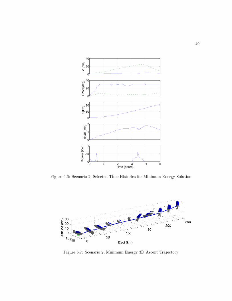
49
0
20
40
V [m
/s]
0
20
40F
PA
γ [d
eg]
0
10
20
h [k
m]
0
1
2
dh/d
t [m
/s]
0 1 2 3 4 50
0.5
1
Pow
er (
kW)
Time (hours)
Figure 6.6: Scenario 2, Selected Time Histories for Minimum Energy Solution
Figure 6.7: Scenario 2, Minimum Energy 3D Ascent Trajectory

50
0
5
10
Thr
ust [
kN]
−10
−5
0
α [d
eg]
−100
0
100
µ [d
eg]
0 2 4 6 8 10 12−200
0
200
ψ [d
eg]
Time [hrs]
Figure 6.8: Scenario 1, Control History for Minimum Energy Solution
6 Time and Energy Tradeoff
For scenarios 1 and 2, we now consider minimum energy trajectories at a series of
specified flight times, extending to a maximum flight time of 12 hours. Figure 6.12
shows the initially steep and then gradual energy reduction with increasing flight time
for both scenarios. For scenario 1, the energy continues to decrease with increasing the
flight time, but extending the flight to 16 hours provides only a 2.5% further decrease in
energy. The minimum energy solutions of scenario 1 follow a similar path to that of the
minimum time case, but climb at slower airspeeds to reduce drag, which results in the
jet stream winds carrying the airship further east. In all cases, the optimal trajectory
involves a direct climb to the maximum operational altitude of 24 km, followed by a
cruise and descent to the target station.
For the minimum energy trajectories of scenario 2, there is a steep decline in the
energy requirement from 2 to 4 hours. The energy reaches a minimum between 5 and
6 hours, and then gradually increases with larger flight time. The zoomed-in view of
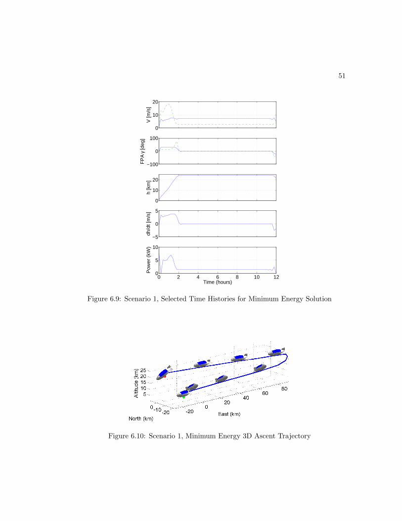
51
0
10
20
V [m
/s]
−100
0
100F
PA
γ [d
eg]
0
10
20
h [k
m]
−5
0
5
dh/d
t [m
/s]
0 2 4 6 8 10 120
5
10
Pow
er (
kW)
Time (hours)
Figure 6.9: Scenario 1, Selected Time Histories for Minimum Energy Solution
Figure 6.10: Scenario 1, Minimum Energy 3D Ascent Trajectory

52
Figure 6.11: Scenario 2, Acceleration Components for Minimum Time and MinimumEnergy Solutions
0 0.5 1 1.5 2−0.05
−0.03
−0.01
0
0.01
0.03
0.05
Time (hours)
Acc
eler
atio
n (m
/s/s
)
Minimum Time
Thrust−DragMass RateWind RateEarth Rot.
0 1 2 3 4 5−5
−3
−1
0
1
3
5x 10
−3
Time (hours)
Acc
eler
atio
n (m
/s/s
)
Minimum Energy
Thrust−DragMass RateWind RateEarth Rot.
0 2 4 6 8 10 120
50
100
150
200
Flight Time (Hours)
En
erg
y (
Kilo
wa
tt−
Ho
urs
)
Scenario 1: 20 km East
Scenario 2: 250 km West
4 5 6 7 8 91
1.2
1.4
1.6
Scenario 2, Zoomed In
Figure 6.12: Scenarios 1 & 2, Energy vs. Time
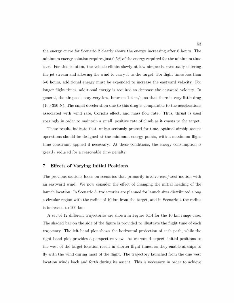
53
the energy curve for Scenario 2 clearly shows the energy increasing after 6 hours. The
minimum energy solution requires just 0.5% of the energy required for the minimum time
case. For this solution, the vehicle climbs slowly at low airspeeds, eventually entering
the jet stream and allowing the wind to carry it to the target. For flight times less than
5-6 hours, additional energy must be expended to increase the eastward velocity. For
longer flight times, additional energy is required to decrease the eastward velocity. In
general, the airspeeds stay very low, between 1-4 m/s, so that there is very little drag
(100-350 N). The small deceleration due to this drag is comparable to the accelerations
associated with wind rate, Coriolis effect, and mass flow rate. Thus, thrust is used
sparingly in order to maintain a small, positive rate of climb as it coasts to the target.
These results indicate that, unless seriously pressed for time, optimal airship ascent
operations should be designed at the minimum energy points, with a maximum flight
time constraint applied if necessary. At these conditions, the energy consumption is
greatly reduced for a reasonable time penalty.
7 Effects of Varying Initial Positions
The previous sections focus on scenarios that primarily involve east/west motion with
an eastward wind. We now consider the effect of changing the initial heading of the
launch location. In Scenario 3, trajectories are planned for launch sites distributed along
a circular region with the radius of 10 km from the target, and in Scenario 4 the radius
is increased to 100 km.
A set of 12 different trajectories are shown in Figure 6.14 for the 10 km range case.
The shaded bar on the side of the figure is provided to illustrate the flight time of each
trajectory. The left hand plot shows the horizontal projection of each path, while the
right hand plot provides a perspective view. As we would expect, initial positions to
the west of the target location result in shorter flight times, as they enable airships to
fly with the wind during most of the flight. The trajectory launched from the due west
location winds back and forth during its ascent. This is necessary in order to achieve
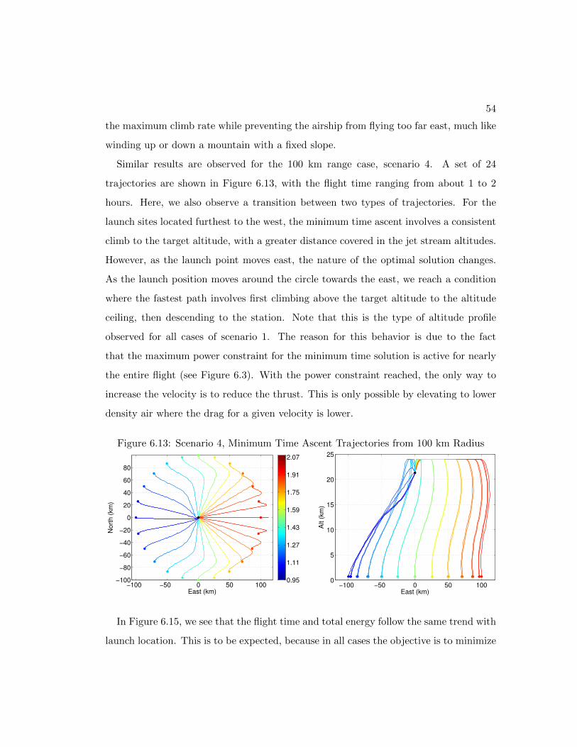
54
the maximum climb rate while preventing the airship from flying too far east, much like
winding up or down a mountain with a fixed slope.
Similar results are observed for the 100 km range case, scenario 4. A set of 24
trajectories are shown in Figure 6.13, with the flight time ranging from about 1 to 2
hours. Here, we also observe a transition between two types of trajectories. For the
launch sites located furthest to the west, the minimum time ascent involves a consistent
climb to the target altitude, with a greater distance covered in the jet stream altitudes.
However, as the launch point moves east, the nature of the optimal solution changes.
As the launch position moves around the circle towards the east, we reach a condition
where the fastest path involves first climbing above the target altitude to the altitude
ceiling, then descending to the station. Note that this is the type of altitude profile
observed for all cases of scenario 1. The reason for this behavior is due to the fact
that the maximum power constraint for the minimum time solution is active for nearly
the entire flight (see Figure 6.3). With the power constraint reached, the only way to
increase the velocity is to reduce the thrust. This is only possible by elevating to lower
density air where the drag for a given velocity is lower.
Figure 6.13: Scenario 4, Minimum Time Ascent Trajectories from 100 km Radius
−100 −50 0 50 100−100
−80
−60
−40
−20
0
20
40
60
80
East (km)
Nort
h (
km
)
0.95
1.11
1.27
1.43
1.59
1.75
1.91
2.07
−100 −50 0 50 1000
5
10
15
20
25
East (km)
Alt (
km
)
In Figure 6.15, we see that the flight time and total energy follow the same trend with
launch location. This is to be expected, because in all cases the objective is to minimize
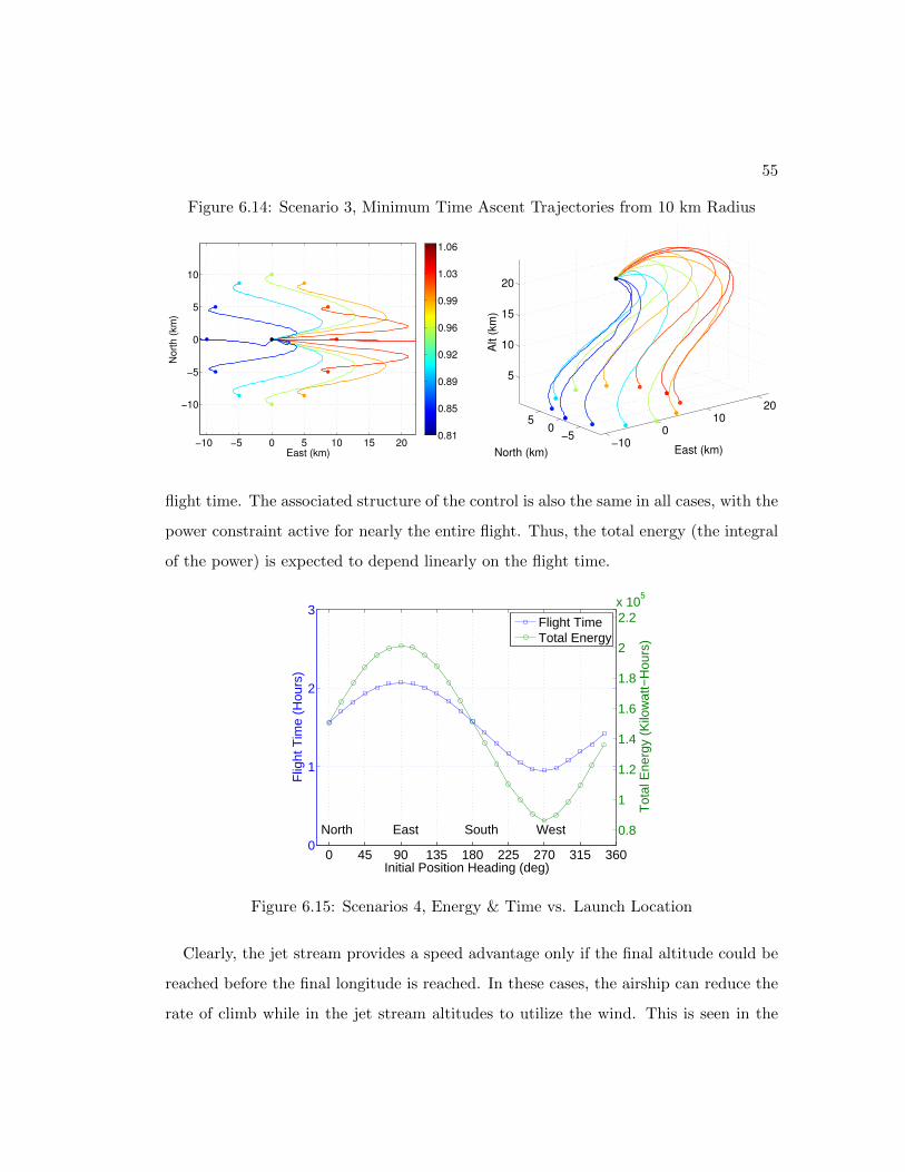
55
Figure 6.14: Scenario 3, Minimum Time Ascent Trajectories from 10 km Radius
−10 −5 0 5 10 15 20
−10
−5
0
5
10
East (km)
Nort
h (
km
)
0.81
0.85
0.89
0.92
0.96
0.99
1.03
1.06
−100
1020
−50
5
5
10
15
20
East (km)North (km)
Alt (
km
)flight time. The associated structure of the control is also the same in all cases, with the
power constraint active for nearly the entire flight. Thus, the total energy (the integral
of the power) is expected to depend linearly on the flight time.
0 45 90 135 180 225 270 315 3600
1
2
3
Initial Position Heading (deg)
Flig
ht T
ime
(Hou
rs)
North East South West 0.8
1
1.2
1.4
1.6
1.8
2
2.2x 10
5
Tot
al E
nerg
y (K
ilow
att−
Hou
rs)
Flight TimeTotal Energy
Figure 6.15: Scenarios 4, Energy & Time vs. Launch Location
Clearly, the jet stream provides a speed advantage only if the final altitude could be
reached before the final longitude is reached. In these cases, the airship can reduce the
rate of climb while in the jet stream altitudes to utilize the wind. This is seen in the
56
far west launch locations of scenario 4, and in the minimum time solution of scenario
2. Here, the launch location is far enough away that, with the fastest possible climb,
the final altitude would be reached before the final longitude is reached. Otherwise,
there is no advantage to staying in the jet stream, and the optimal solution is simply to
climb as fast as possible. Since the jet stream winds carry the airship further east of the
target station in these cases, the final phase of the flight involves flying into the wind at
maximum power, and sometimes at maximum airspeed. This final return phase involves
a cruise at the maximum altitude where the resisting wind and density is smallest.
8 Discussions
Results obtained in this paper are specific to the wind model and airship configuration
that was used. However, the wind model is representative of the class of wind profiles
that are seen throughout many parts of the globe, and the airship design is based upon
published data from prototype vehicles as well as accumulated engineering experience
from prior work in airship research. Therefore, examination of these optimization results
enables us to develop some general strategies for planning optimal ascent trajectories
subject to similar wind profiles and similar vehicle designs.
There are also some important limitations to the scope of this analysis. First, neutral
buoyancy has been assumed at all flight conditions, which requires the pressure regula-
tion system to achieve high mass flow rates during high rates of climb, or more precisely
whenever the rate of change in the ambient air density is high. A more accurate model
would include air flow constraints, so that buoyancy and weight are modeled separately.
In such a model, neutral buoyancy conditions would only be achieved when the required
mass flow rate is under the prescribed limit. Also, as previously mentioned, our model
for the required power for flight does not include the operation of fans for pressure
regulation. Including this power requirement in the performance objective would lead
to more accurate predictions of energy consumption, and may influence the optimal
trajectories. Finally, the power generation during the flight of a stratospheric airship
57
depends upon its orientation, which governs the incidence angles of the photovoltaic so-
lar cells. Introducing a model for the generated power and including appropriate energy
balance constraints may lead to a different class of optimal trajectories that exploit the
combination of the wind-relative and inertial orientations as the sun moves through the
sky. Each of these areas are topics worthy of future research.
Chapter 7
Performance Evaluation of
Optimal Solutions
7.1 Introduction
In this chapter, we seek to analyze some performance aspects of the optimal ascent
trajectories developed earlier. Two different types of analyses are conducted. First, we
develop a model to compute the solar flux available to the airship, and use this model to
approximate the solar power and cumulative energy that the airship can generate during
an ascent trajectory. This analysis is performed for a variety of ascent trajectories in
order to identify how the vehicle orientation and flight profile can impact its power
production, and to determine whether batteries are needed for ascent. Solar power
modeling for airships has been presented before [3, 4, 5, 29], but the analysis here
provides a more general model that includes seasonal and diurnal effects, hull geometry
effects, atmospheric losses, and the attitude of the vehicle.
In the second analysis, we consider changes to the drag coefficient and the wind model,
and attempt to quantify how these changes impact the performance of the optimal
trajectories. To do this we conduct a new series of trajectory optimizations, each with
58

59
respect to a different model perturbation. This exercise allows us to determine the
sensitivity of the optimal solutions to changes in uncertain parameters.
7.2 Energy Production Analysis
Optimal ascent trajectories have been developed for a variety of different scenarios.
Minimum time and minimum energy flights were planned from launch sites located
downwind and upwind of the target station, and minimum time flights were found for
an array of launch sites that surrounded the target station. It was found that minimum-
time flights spend much of their time operating at the maximum power constraint, which
was set at 100 kW to match the conceptual design in Ref. [2]. Given the large amount
of energy required for these flights, it is important to understand how much energy can
be supplied from solar power. If the solar energy production is insufficient for daytime
ascents, batteries will be required.
In this section, we use the solar flux model developed in Section 3.5 to analyze the
energy production capability associated with a set of optimal trajectories from Ref. [17].
A plot of the minimum time trajectories for 24 launch sites at a 100 km radius from
the target station is shown in Figure 6.13. The flight paths are shaded according to the
flight times, shown in hours in the shaded legend bar.
The propulsion energy required for each trajectory is
EReq =
∫ tF
t0
TV
ηPdt
where ηP is the combined efficiency of the electric motor and propellers. For this analysis
we let ηP = 0.65.
The solar energy that may be generated for each trajectory is
EGen = ηS
∫ tF
t0
Fdt
where F is the total solar flux from Eq. (3.64), and ηS is the efficiency of the solar cells.
In truth, the efficiency of all cells cannot be accurately modeled as a single parameter.
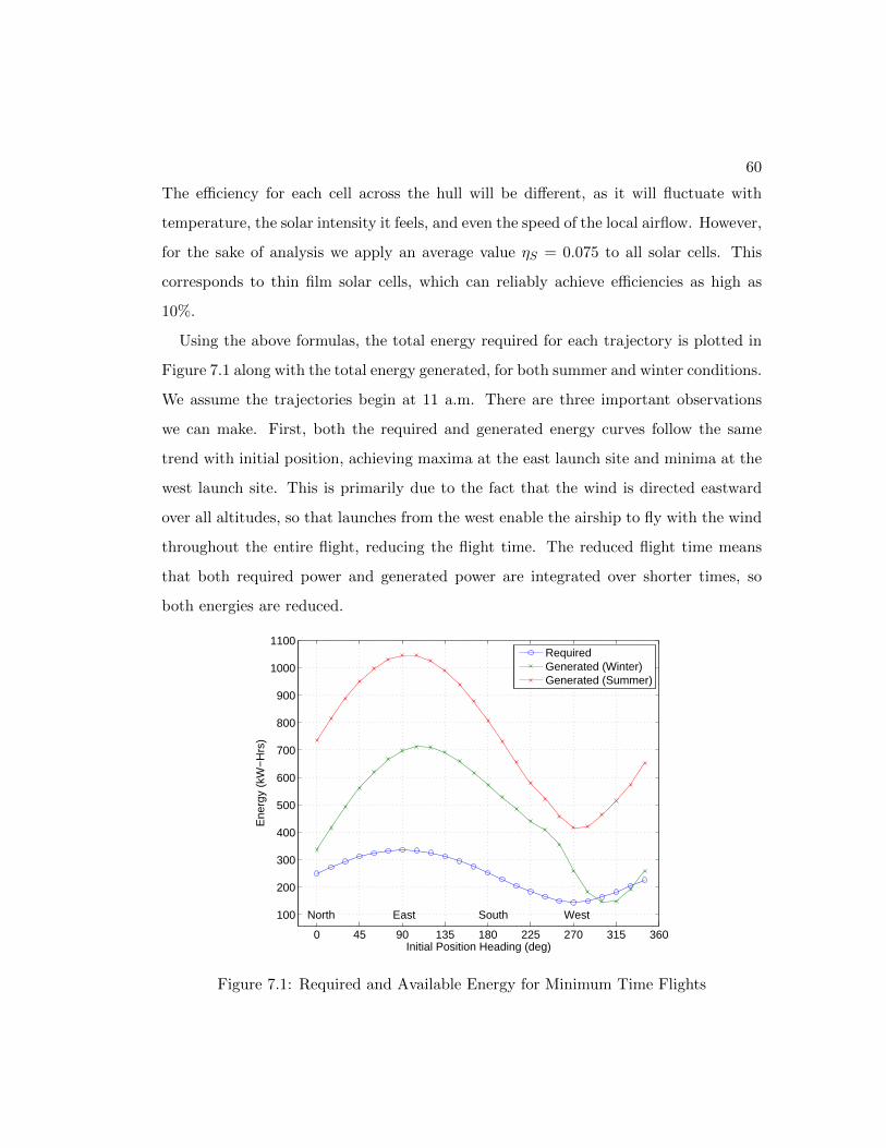
60
The efficiency for each cell across the hull will be different, as it will fluctuate with
temperature, the solar intensity it feels, and even the speed of the local airflow. However,
for the sake of analysis we apply an average value ηS = 0.075 to all solar cells. This
corresponds to thin film solar cells, which can reliably achieve efficiencies as high as
10%.
Using the above formulas, the total energy required for each trajectory is plotted in
Figure 7.1 along with the total energy generated, for both summer and winter conditions.
We assume the trajectories begin at 11 a.m. There are three important observations
we can make. First, both the required and generated energy curves follow the same
trend with initial position, achieving maxima at the east launch site and minima at the
west launch site. This is primarily due to the fact that the wind is directed eastward
over all altitudes, so that launches from the west enable the airship to fly with the wind
throughout the entire flight, reducing the flight time. The reduced flight time means
that both required power and generated power are integrated over shorter times, so
both energies are reduced.
0 45 90 135 180 225 270 315 360
100
200
300
400
500
600
700
800
900
1000
1100
Initial Position Heading (deg)
Ene
rgy
(kW
−H
rs)
North East South West
RequiredGenerated (Winter)Generated (Summer)
Figure 7.1: Required and Available Energy for Minimum Time Flights

61
The second observation we can make is that for the winter case, the generated power
drops sharply for launch sites between 270 deg and 360 deg. This is because the airship
is climbing at a pitch angle of 30-40 degrees during ascent, and for these launch sites,
the vehicle is facing a southern direction. Thus, at this northern latitude in the winter,
the inclined pitch angle with a south heading blocks much of the top-mounted solar cells
from the sun.
Finally, we see that the energy generated for nearly all flights considered surpasses the
energy requirement. This provides confirmation that the baseline design configuration
should adequately meet the energy demands of minimum-time ascent trajectories. How-
ever, these results are based upon an assumption of constant efficiency for the motors,
propellers, solar cells. If the true efficiencies are significantly below the assumed values,
then solar energy production may prove insufficient for these minimum-time flights.
1 Energy Requirement for Ballast Control
The energy requirement considered thus far is limited to that required for propulsion. It
is instructive to also consider the energy required to move air in and out of the ballonets.
To do so, we develop a simple model which provides a reasonable approximation. If the
mass flow rate is directed vertically down, then the force associated with the air flow is
|mh|. This force must act over each incremental change in altitude. The total energy
required for ballast control, therefore, is the work done by this force over altitude.
Letting dh = hdt, the expression becomes:
EBC =
∫ tF
t0
|m|h2dt
For neutral buoyancy, the mass of the enclosed airship (including ballast air in the
ballonets) must equal the mass of displaced air. The mass flow rate of the airship is
therefore equivalent to the mass rate of change of the displaced air:
m = UH ρ
= UH∂ρ
∂hh (7.1)
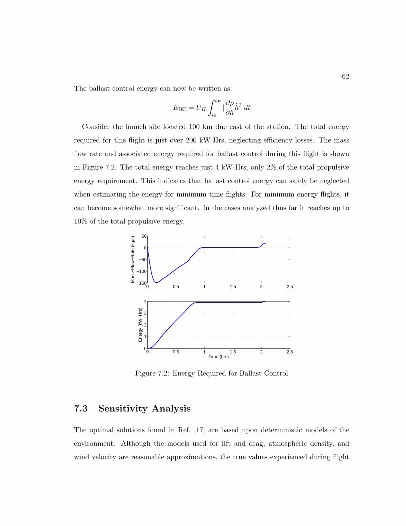
62
The ballast control energy can now be written as:
EBC = UH
∫ tF
t0
|∂ρ∂hh3|dt
Consider the launch site located 100 km due east of the station. The total energy
required for this flight is just over 200 kW-Hrs, neglecting efficiency losses. The mass
flow rate and associated energy required for ballast control during this flight is shown
in Figure 7.2. The total energy reaches just 4 kW-Hrs, only 2% of the total propulsive
energy requirement. This indicates that ballast control energy can safely be neglected
when estimating the energy for minimum time flights. For minimum energy flights, it
can become somewhat more significant. In the cases analyzed thus far it reaches up to
10% of the total propulsive energy.
0 0.5 1 1.5 2 2.5−150
−100
−50
0
50
Mas
s−F
low
−R
ate
(kg/
s)
0 0.5 1 1.5 2 2.50
1
2
3
4
Time (hrs)
Ene
rgy
(kW
−H
rs)
Figure 7.2: Energy Required for Ballast Control
7.3 Sensitivity Analysis
The optimal solutions found in Ref. [17] are based upon deterministic models of the
environment. Although the models used for lift and drag, atmospheric density, and
wind velocity are reasonable approximations, the true values experienced during flight
63
will differ from these simplistic models. This is especially true for the wind model, as
the actual wind profile for a given day may be quite different from the representative
model selected for planning.
It is therefore important to examine the sensitivity of the optimal solutions to changes
in model parameters. In this section we present the results from a sensitivity analysis
conducted with respect to independent changes in the drag coefficient and the wind
profile. Two different optimal flight plans are considered:
1. Minimum-time flight from a launch site 250 km west of the station
2. Minimum-time flight from a launch site 20 km east of the station
The characteristics of the optimal solutions for these two scenarios are discussed ex-
tensively in Ref. [17]. In this sensitivity analysis, we introduce small changes to the
drag coefficient and wind profile, and then recompute the minimum-time solutions with
respect to the changed models. The sensitivity of flight time and total energy consump-
tion for each new trajectory is then illustrated by plotting their changing values against
the varying model parameters.
1 Variation in Drag Coefficient
The nominal drag coefficient at zero incidence is 0.04, based upon the aerodynamic
model presented in Ref. [2]. We consider a ±50% change in the drag coefficient, so
that it can range between 0.02 and 0.06. The sensitivity of flight time and total energy
consumption is shown in Figure 7.3.
The results show a relatively small sensitivity to the drag coefficient. For a ±10%
change in drag coefficient around 0.04, the optimal flight time for the east launch site
changes by about 3.3 minutes, compared with about 1.9 minutes for the west launch
site. This is a 5% change for the east site, and only a 1.5% change for the west site.
The energy sensitivity follows a similar trend. This is expected as the total energy is
roughly proportional to flight time.

64
Figure 7.3: Sensitivity of Flight Time and Energy to Drag Coefficient
1.8
1.9
2.0
2.1
2.2
2.3
2.4
Flig
ht
Tim
e (
Hrs
)
−−
x −
−
250 km West
20 km East
0.2 0.25 0.3 0.35 0.4 0.45 0.5 0.55 0.60.8
0.9
1.0
1.1
1.2
1.3
1.4
Drag Coefficient
Flig
ht
Tim
e (
Hrs
)
−−
o −
−
Flight Time
160
180
200
220
En
erg
y (
kW
−H
rs)
−
− x
−−
250 km West
20 km East
0.2 0.25 0.3 0.35 0.4 0.45 0.5 0.55 0.6 70
90
110
130
En
erg
y (
kW
−H
rs)
−
− o
−−
Drag Coefficient
Energy
The east launch site trajectories are more sensitive to drag coefficient because they
fly at a higher average airspeed velocity. This can be explained by examining the 2D
optimal flight paths, shown in Figure 7.4. The trajectories for both cases follow a
consistent structure. For the west launch site, the optimal solution is to climb at max
power and at max flight path angle until the jet stream altitude is reached, at which
point the airship cruises at max power until finally climbing to the station. Because
it is already at the maximum power constraint, it cannot increase velocity or thrust,
and it cruises at an airspeed of about 17.2 m/s. For the east launch site case, it climbs
at the max rate of climb all the way to the target station, increasing airspeed as it
goes. It therefore has a higher average airspeed. As drag is proportional to the square
of the airspeed, these trajectories are more strongly influenced by changes in the drag
coefficient.
2 Variation in Peak Wind Magnitude
The nominal wind profile is based on the HWM93 model for the winter season above
Edwards AFB in California, as shown in Figure 3.5. Let us denote this curve as WE(h).
We consider incremental changes to this nominal profile by introducing a wind variation

65
Figure 7.4: Variation of Optimal Flight Paths with Drag Coefficient
−250 −200 −150 −100 −50 00
5
10
15
20
25
Station
West Launch Site
IncreasingDrag
East (km)
Alti
tude
(km
)
−10 0 10 20 30 400
5
10
15
20
25
Station
East Launch Site
IncreasingDrag
East (km)
Alti
tude
(km
)
δWE , so that
WE(h) = WE(h) + δWE(h)
The variation is defined as: which is a Gaussian distribution centered at hmax with height
∆Wp, and spread across an altitude range of ∆h. This enables us to add a smooth
variation to the original wind profile, with a desired magnitude change located at a
particular altitude. We choose to add the magnitude change at hmax = 12 km, which
is the altitude of peak wind speed, and we consider 8 different magnitude variations
ranging from ∆Wp = −5 to +5 m/s. The resulting curve is then fit with a new 7th
order polynomial . The curves for all polynomial fits are shown in Figure 7.5.
The sensitivities are shown in Figure 7.6. For the west launch site, increases in the
eastward wind reduce the flight time and energy, while they are increased for the east
launch site. Again, the sensitivities are relatively small. The flight time and energy for
the west site drop by about 1.7% for each 1 m/s increase in the peak wind magnitude.
This compares to about 1.0% increase in flight time and energy for the east site.
The 2D optimal flight paths are shown in Figure 7.7. Again, the trajectories follow
a consistent structure. For the east launch site, the optimal solution in every case is to
climb to the pressure altitude, fly back towards the station, then descend to the target
altitude. With the max power constraint reached, the only way to increase the velocity
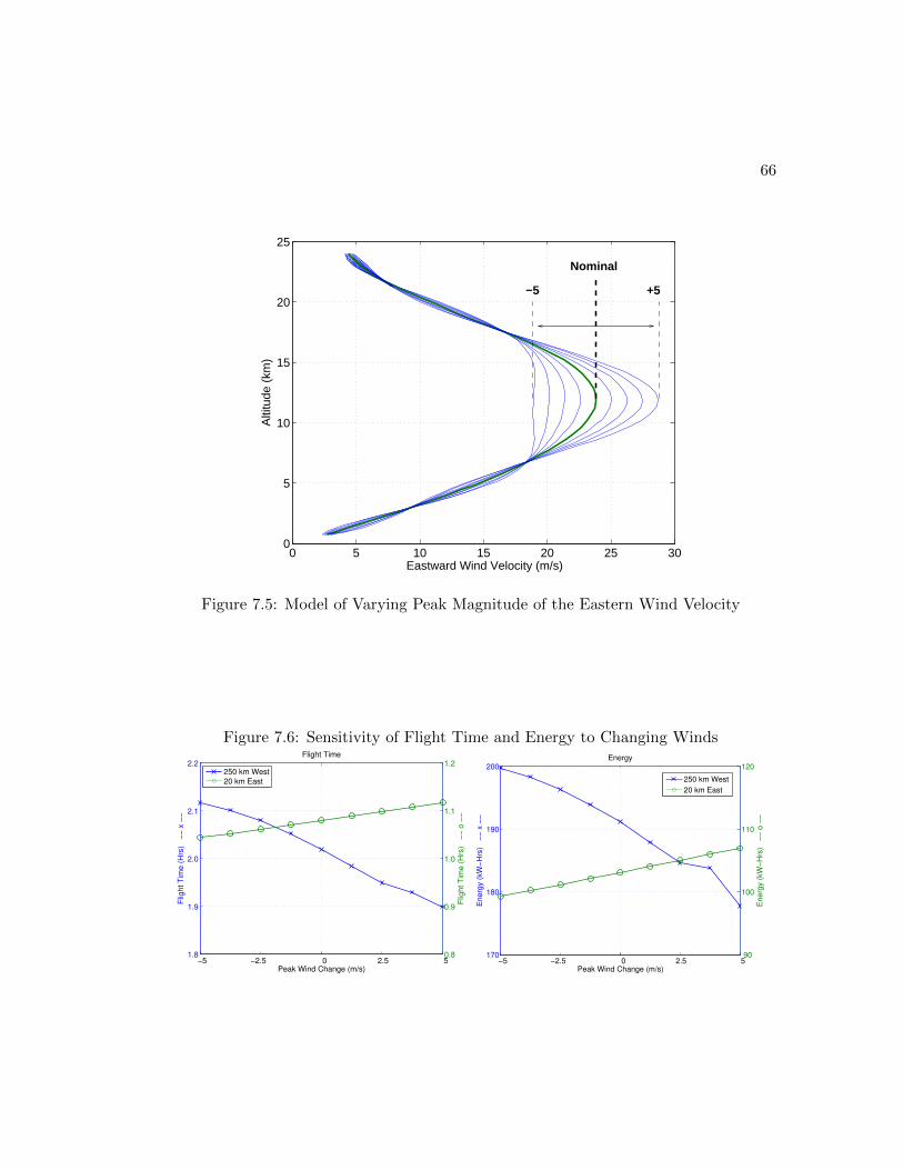
66
0 5 10 15 20 25 300
5
10
15
20
25
Eastward Wind Velocity (m/s)
Alti
tude
(km
)Nominal
−5 +5
Figure 7.5: Model of Varying Peak Magnitude of the Eastern Wind Velocity
Figure 7.6: Sensitivity of Flight Time and Energy to Changing Winds
1.8
1.9
2.0
2.1
2.2
Flig
ht
Tim
e (
Hrs
)
−−
x −
−
250 km West
20 km East
−5 −2.5 0 2.5 50.8
0.9
1.0
1.1
1.2
Peak Wind Change (m/s)
Flig
ht
Tim
e (
Hrs
)
−−
o −
−
Flight Time
170
180
190
200
En
erg
y (
kW
−H
rs)
−
− x
−−
250 km West
20 km East
−5 −2.5 0 2.5 5 90
100
110
120
Peak Wind Change (m/s)
En
erg
y (
kW
−H
rs)
−
− o
−−
Energy

67
is to reduce the thrust. This is only possible by elevating to lower density air where the
drag for a given velocity is lower.
The same principle applies for the west launch site trajectories. The maximum wind
speed is always located at about 12 km altitude. It would seem that this would be the
ideal altitude for the airship to cruise at until it comes close to the station. However,
it can reach a higher airspeed velocity at higher altitudes with lower density, and so it
climbs above 12 km. It cannot climb to far, though, as the contribution from the wind
speed begins to drop. The cruise altitude in each scenario is therefore the location of
the maximum possible total velocity. The airship climbs higher for wind profiles with
smaller peaks because the increase in airspeed remains larger than the decrease in wind
speed over a larger altitude range.
Figure 7.7: Variation of Optimal Flight Paths with Changing Winds
−250 −200 −150 −100 −50 00
5
10
15
20
25
Station
West Launch Site
IncreasingWind
East (km)
Alti
tude
(km
)
−10 0 10 20 30 400
5
10
15
20
25
Station
East Launch Site
IncreasingWind
East (km)
Alti
tude
(km
)
7.4 Concluding Remarks
A model for the solar flux of an ellipsoidal airship hull has been developed, which includes
the effects due to geographic latitude, seasonal and diurnal effects that govern the sun
motion, the curvature loss for an ellipsoidal hull, and the time-varying orientation of the
airship. This model was used to analyze the energy production associated with several
68
minimum-time ascent trajectories. We find that the energy production capability is
sufficiently high to meet the energy demands for these trajectories, assuming a mid-day
launch time. However, it is also discovered that the steep pitch angle during ascent can
result in significant energy loss for certain orientations, particularly south-flying ascents
from the northern hemisphere, and vice versa. The sensitivity of the optimal solutions
is also examined with respect to changes in drag coefficient and peak wind magnitude.
The flight time and total energy of the flights are found to change by only a few percent,
and the optimal trajectories retain a consistent structure over all parameter values.

Chapter 8
Onboard Guidance Methods
8.1 Introduction
Optimal ascent trajectories have been presented here and in previous works [2, 17]. The
optimal ascent trajectories in Chapter 6 have been found through the numerical solution
of optimal control problems. Solutions were obtained by first using collocation to dis-
cretize the optimal control problem over a finite number of time intervals, producing a
nonlinear parameter optimization problem where nonlinear equality constraints are used
to capture the dynamic equations. Each discrete formulation consists of hundreds to
thousands of variables and nonlinear constraint equations, requiring a substantial com-
putational effort to reach a solution. In addition, as is often the case in high-dimension
nonlinear optimization, reliable convergence requires a good initial guess, which is not
trivial to construct. Considering the computational demands and the risk of not obtain-
ing feasible solutions in time to use them, this approach is not well-suited for onboard
implementation. One way to implement a form of optimal guidance onboard without
this prohibitively high computational burden is by first generating optimal solutions
offline. However, in this case each optimal solution would be valid only for a single wind
model. Because the wind profile across altitude is uncertain, it would be necessary to
69

70
pre-compute optimal trajectories for a large number of possible wind profiles.
In this section, an alternative guidance method is presented in which approximate
optimal trajectories are solved. By characterizing the structure of the original opti-
mal solutions, minimum-time and minimum-energy ascent flights are approximated by
piecing together different parameterized flight segments. This greatly simplifies the
optimization, leaving only a small number of variables to be decided.
The guidance and control system structure is shown in Figure 8.1. Wind measure-
ments are used to update the onboard wind model, which fits a combination of recorded
winds at lower altitudes and the current wind predictions at higher altitudes into a
polynomial function. The predicted wind profile and current states are used in an outer
loop guidance strategy to determine the desired airspeed, flight path, heading, and al-
titude. Nonlinear dynamic inversion is then used to command the thrust, thrust pitch
angle, and angle of attack in order to track the desired trajectory.
WE
WN
WN
AirshipDynamics
NDIInner Loop
Vγ
hλℓ
Tµα
TargetStation
Optimal Strategy
Outer Loop
htgt γc
Vc
OnboardWind Model
ψc
TrueWind Model
WE(h)
dWE / dt
dWN / dt
h
Estimatewith Sensors
and GPSWN(h)
WE
λtgt
ℓtgt
Figure 8.1: Control System Architecture
71
The onboard guidance strategy integrates an onboard wind model across a candidate
altitude profile to predict a wind-relative location for the target station. Thisvirtual
target station moves gradually as the wind model is updated.
The next section discusses nonlinear dynamic inversion as a guidance method, and
how it is applied to our airship dynamic model. The section that follows describes the
concept of the virtual target and how it is used in planning optimal ascents.
8.2 Dynamic Inversion
This section describes the use of non-linear dynamic inversion as a feedback control
method for autonomous guidance. The goal is to develop a suitable framework for
evaluating the performance of the optimal trajectory solutions in closed-loop simula-
tions. As such, the scope is limited to controlling the point mass model of the airship
so that it tracks the optimal trajectory. It should be pointed out that the full design
of an autonomous guidance system for stratospheric airships would include also GPS
navigation, local state estimation, wind estimation, and the use of actuators to control
the airship state. However, for the present analysis it is assumed that each of these
components may be designed to function sufficiently. The research is instead focused
on measuring how deviations from the predicted wind profile will impact the ability of
the airship to follow the optimal trajectory, and in general how it will impact certain
measures of performance in the closed-loop trajectory.
The concept of dynamic inversion is to define the control signal input so that it
produces desired dynamics. If the desired dynamics are linear, then the approach may
also be referred to as feedback linearization. Consider a general dynamic system with
state x, output y and input u. We first consider a linear system:
x = Ax+Bu (8.1)
y = Cx (8.2)
Next, the control signal may be expressed in terms of the output dynamics and the
72
state:
u = (CB)−1 (Cx− CAx) (8.3)
= (CB)−1 (y − CAx) (8.4)
Let ydes be the desired time derivative of the output y. Dynamic inversion involves
solving for the control signal that achieves the desired output dynamics. The solution
is found simply by substituting the desired signal ydes for the y term in Eq. 8.4.
uc = (CB)−1 (ydes − CAx)
Note that the above equation requires matrix CB to be nonsingular. If it is singular,
then one may instead attempt to track the second derivative, y, which requires the
inverse of matrix CAB.
If the system is nonlinear, it may be expressed as follows:
x = f(x, u) (8.5)
y = h(x) (8.6)
The output dynamics are found through the chain rule:
y =∂h
∂xx (8.7)
=∂h
∂xf(x, u) (8.8)
As before, we now use this equation to solve for u in terms of x and y. Let this
solution be expressed in general form as u = g(x, y). The control signal solution for
nonlinear dynamic inversion is then:
uc = g(x, ydes)
Whether the dynamic system to be controlled is linear or non-linear, the dynamic
inversion method requires the desired signal ydes to be defined.

73
1 Airship Dynamic Model
The nonlinear dynamic equations for the airship point mass vehicle are given below:
h = V sin γ (8.9)
λ =V cos γ cosψ +WN
R+ h(8.10)
˙ =V cos γ sinψ +WE
(R+ h) cosλ(8.11)
V =T cosµ− 1
2ρ(h)U2/3H CD(α)V 2 − UH
(δρδh
)hV
m+max− Wx (8.12)
γ =T sinµ+ 1
2ρ(h)U2/3H CL(α)V 2
(m+maz)V− Wz
V(8.13)
Note that in Eq. (8.12), the mass flow rate is expressed as:
m =d
dt(UHρ(h)) (8.14)
= UH ρ(h)
= UH
(∂ρ
∂h
)h
The wind rate terms in the wind frame are:
Wx = WE cos γ sinψ + WN cos γ cosψ (8.15)
Wz = WE sin γ sinψ + WN sin γ cosψ (8.16)
2 Nonlinear Dynamic Inversion for Airship Guidance
The Nonlinear Dynamic Inversion (NDI) approach used for airship guidance was shown
in Figure 8.1. The objective of this design is to track the optimal position trajectory
that is computed offline by the trajectory optimization program. The commanded 3-
dimensional inertial position consists of the altitude hc, latitude λc and longitude `c.
These reference signals are sent to the NDI outer loop control law, which commands
the wind-relative velocity vector necessary to track the reference inertial position. The
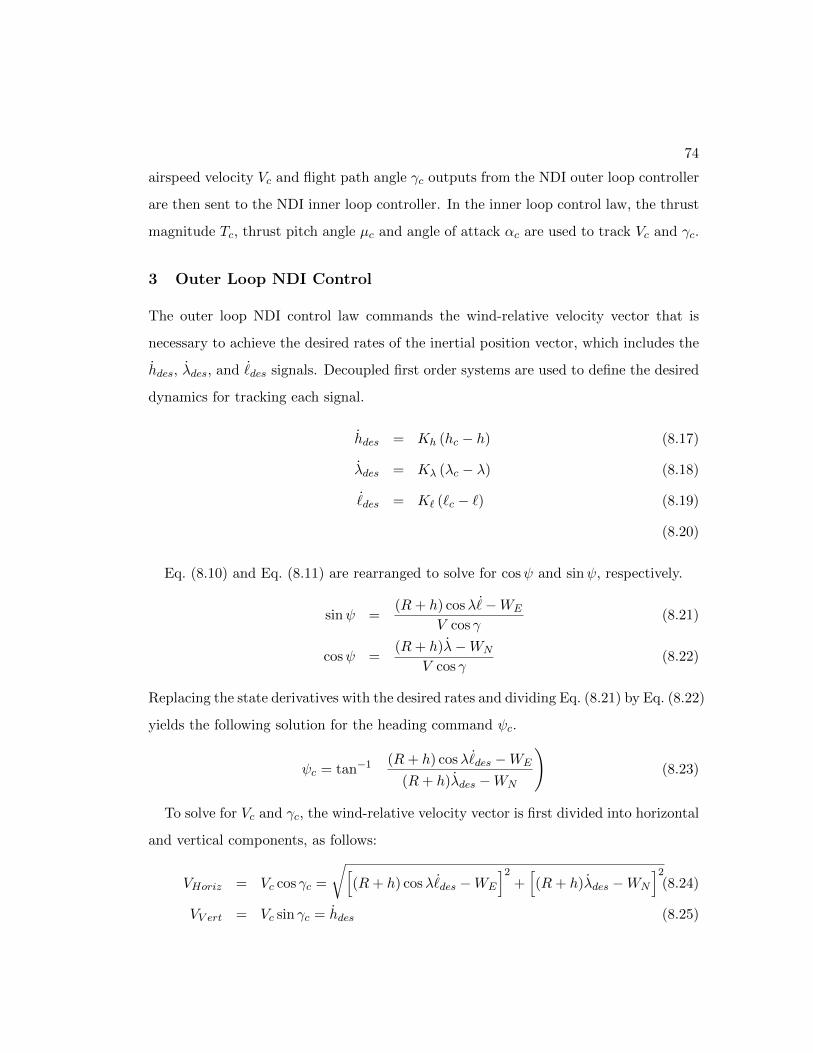
74
airspeed velocity Vc and flight path angle γc outputs from the NDI outer loop controller
are then sent to the NDI inner loop controller. In the inner loop control law, the thrust
magnitude Tc, thrust pitch angle µc and angle of attack αc are used to track Vc and γc.
3 Outer Loop NDI Control
The outer loop NDI control law commands the wind-relative velocity vector that is
necessary to achieve the desired rates of the inertial position vector, which includes the
hdes, λdes, and ˙des signals. Decoupled first order systems are used to define the desired
dynamics for tracking each signal.
hdes = Kh (hc − h) (8.17)
λdes = Kλ (λc − λ) (8.18)
˙des = K` (`c − `) (8.19)
(8.20)
Eq. (8.10) and Eq. (8.11) are rearranged to solve for cosψ and sinψ, respectively.
sinψ =(R+ h) cosλ ˙−WE
V cos γ(8.21)
cosψ =(R+ h)λ−WN
V cos γ(8.22)
Replacing the state derivatives with the desired rates and dividing Eq. (8.21) by Eq. (8.22)
yields the following solution for the heading command ψc.
ψc = tan−1
((R+ h) cosλ ˙
des −WE
(R+ h)λdes −WN
)(8.23)
To solve for Vc and γc, the wind-relative velocity vector is first divided into horizontal
and vertical components, as follows:
VHoriz = Vc cos γc =
√[(R+ h) cosλ ˙
des −WE
]2+[(R+ h)λdes −WN
]2(8.24)
VV ert = Vc sin γc = hdes (8.25)

75
Dividing Eq. (8.25) by Eq. (8.24) yields a solution for the commanded flight path angle:
γc = tan−1
hdes√[(R+ h) cosλ ˙
des −WE
]2+[(R+ h)λdes −WN
]2
(8.26)
Finally, computing the magnitude of the horizontal and vertical components yields an
expression for the airspeed command.
Vc =
√[(R+ h) cosλ ˙
des −WE
]2+[(R+ h)λdes −WN
]2+ h2
des (8.27)
Equations (8.23,8.26,8.27) define the wind-relative velocity vector command that is
output from the outer loop NDI control law.
4 Inner Loop NDI Control
The inner loop NDI control law commands the thrust magnitude Tc, thrust pitch angle
µc and angle of attack αc in order to track the commanded wind-relative velocity com-
ponents: Vc, γc. A diagram of the inner loop NDI control law is shown in Figure 8.2.
The first-order desired dynamics for the inner-loop are:
Vdes = KV (Vc − V ) (8.28)
γdes = Kγ (γc − γ) (8.29)
ψdes = Kψ (ψc − ψ) (8.30)
Let the body frame x and z components of the thrust command be Tx = Tc cosµc
and Tz = Tc sinµc. We solve for these quantities directly by using the desired signals
Vdes and γdes in Eq. (8.12) and Eq. (8.13), respectively.
Tx = (m+max)(Vdes + Wx + aEx
)+
1
2ρ(h)U
2/3H CD(αc)V
2 + UH(∂ρ
∂h)hV(8.31)
Tz = (m+maz)(V γdes − Wz − aEz
)− 1
2ρ(h)U
2/3H CL(αc)V
2 (8.32)
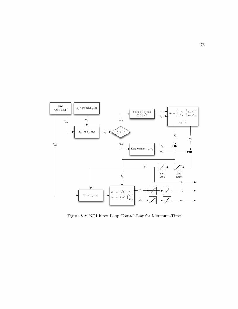
76
RateLimit
Pos.Limit
Vdes
Tx Tx ≥ 0 ?Tx = f ( Vc , αc)
αc = arg min CD(α)
αc
NDI Outer Loop
γdes
Tz = f ( γc , αc)
Solve α1, α2 for:Tx (α) = 0
Keep Original Tx , αc
Tx = 0NO
YES
α1
α2
αc
αc
αc
Tx
Tx
αc
Tx
Tc
µc
Tc
µc
↵c =
↵1 hdes < 0
↵2 hdes 0
Tc =p
T 2x + T 2
z
µc = tan1
Tz
Tx
Figure 8.2: NDI Inner Loop Control Law for Minimum-Time
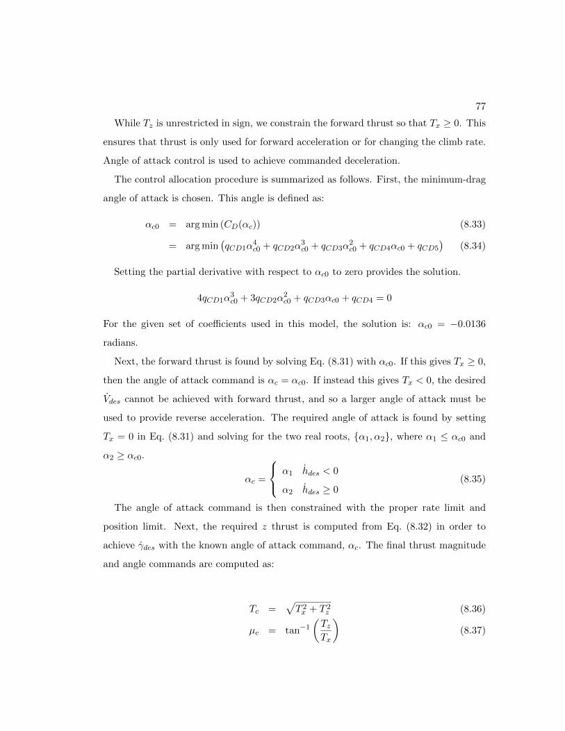
77
While Tz is unrestricted in sign, we constrain the forward thrust so that Tx ≥ 0. This
ensures that thrust is only used for forward acceleration or for changing the climb rate.
Angle of attack control is used to achieve commanded deceleration.
The control allocation procedure is summarized as follows. First, the minimum-drag
angle of attack is chosen. This angle is defined as:
αc0 = arg min (CD(αc)) (8.33)
= arg min(qCD1α
4c0 + qCD2α
3c0 + qCD3α
2c0 + qCD4αc0 + qCD5
)(8.34)
Setting the partial derivative with respect to αc0 to zero provides the solution.
4qCD1α3c0 + 3qCD2α
2c0 + qCD3αc0 + qCD4 = 0
For the given set of coefficients used in this model, the solution is: αc0 = −0.0136
radians.
Next, the forward thrust is found by solving Eq. (8.31) with αc0. If this gives Tx ≥ 0,
then the angle of attack command is αc = αc0. If instead this gives Tx < 0, the desired
Vdes cannot be achieved with forward thrust, and so a larger angle of attack must be
used to provide reverse acceleration. The required angle of attack is found by setting
Tx = 0 in Eq. (8.31) and solving for the two real roots, α1, α2, where α1 ≤ αc0 and
α2 ≥ αc0.
αc =
α1 hdes < 0
α2 hdes ≥ 0(8.35)
The angle of attack command is then constrained with the proper rate limit and
position limit. Next, the required z thrust is computed from Eq. (8.32) in order to
achieve γdes with the known angle of attack command, αc. The final thrust magnitude
and angle commands are computed as:
Tc =√T 2x + T 2
z (8.36)
µc = tan−1
(TzTx
)(8.37)

78
As with the angle of attack, each of these commands is constrained by its rate and
position limit.
Minimizing Thrust Magnitude
The angle of attack command provides an additional degree of freedom. This enables
the thrust magnitude to be minimized subject to the above equations, leading to the
following convex, constrained minimization:
minαc
Tx(αc)2 + Tz(αc)
2 (8.38)
subject to Tx(αc) ≥ 0
αmin ≤ αc ≤ αmax
where Tx(αC) and Tz(αC) are given by Eq. (8.31) and Eq. (8.32), respectively.
The solution to the unconstrained problem is found by setting the gradient of the
cost function to zero. This reduces to:
d
dαc
(Tx(αc)
2 + Tz(αc)2)
= 0 (8.39)
TxT′x + TzT
′z = 0 (8.40)
where T ′x and T ′z are the partial derivatives with respect to αc of Tx and Tz, respectively.
The only dependence on αc appears in the lift and drag coefficients. Therefore these
derivatives are:
T ′x =1
2ρ(h)U
2/3H V 2 d
dαc(CD(αc)) (8.41)
T ′z = −1
2ρ(h)U
2/3H V 2 d
dαc(CL(αc)) (8.42)
Both the lift and drag coefficients are approximated as 4th
order polynomials in α, and
so their derivatives with respect to α are 3rd
order polynomials. Therefore, Eq. (8.40) is
a 7th
order polynomial whose roots contain the optimal unconstrained solution. Alter-
natively, the solution could be obtained through the use of a gradient search method.
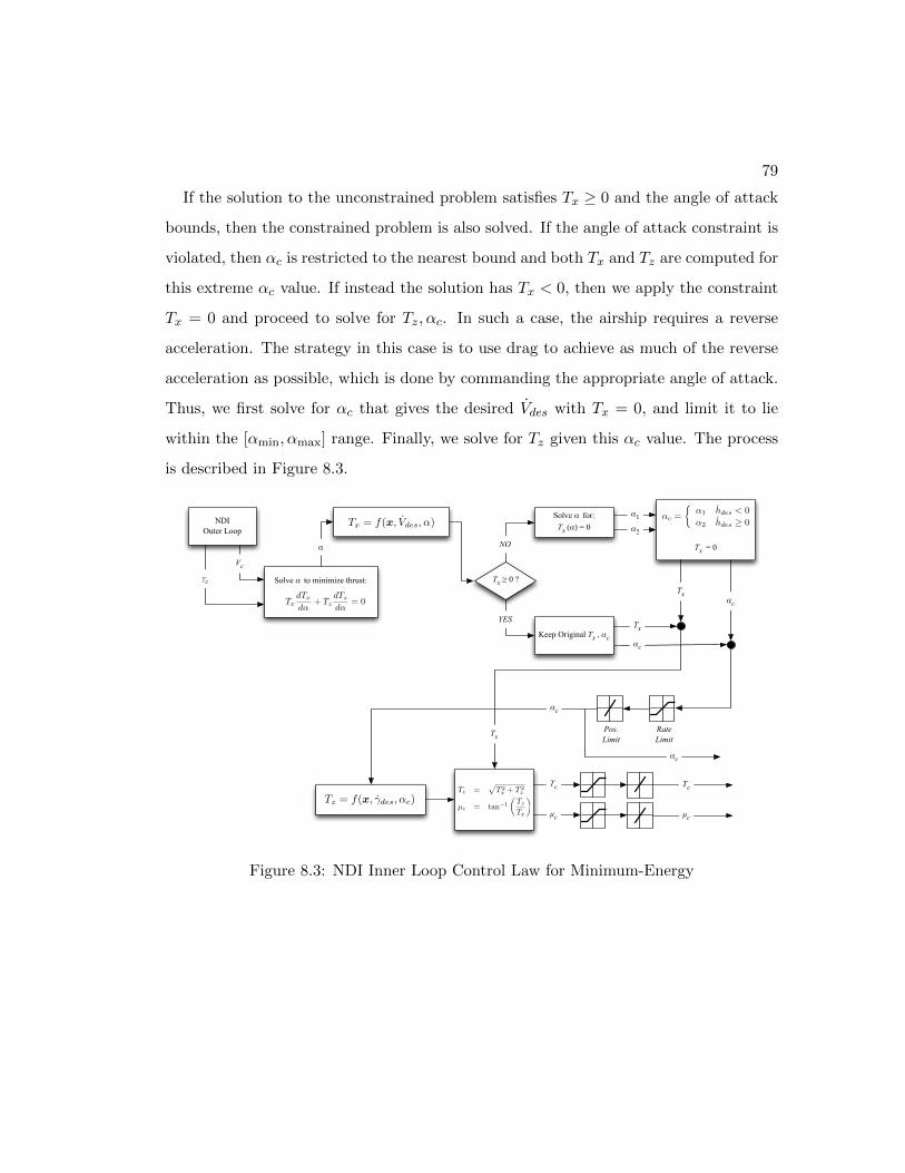
79
If the solution to the unconstrained problem satisfies Tx ≥ 0 and the angle of attack
bounds, then the constrained problem is also solved. If the angle of attack constraint is
violated, then αc is restricted to the nearest bound and both Tx and Tz are computed for
this extreme αc value. If instead the solution has Tx < 0, then we apply the constraint
Tx = 0 and proceed to solve for Tz, αc. In such a case, the airship requires a reverse
acceleration. The strategy in this case is to use drag to achieve as much of the reverse
acceleration as possible, which is done by commanding the appropriate angle of attack.
Thus, we first solve for αc that gives the desired Vdes with Tx = 0, and limit it to lie
within the [αmin, αmax] range. Finally, we solve for Tz given this αc value. The process
is described in Figure 8.3.
RateLimit
Pos.Limit
Vc
Tx ≥ 0 ?
NDI Outer Loop
γc
Solve α for:Tx (α) = 0
Keep Original Tx , αc
Tx = 0NO
YES
α1
α2
αc
αc
αc
Tx
Tx
αc
Tx
Tc
µc
Tc
µc
Solve α to minimize thrust:
TxdTx
d↵+ Tz
dTz
d↵= 0
α
Tc =p
T 2x + T 2
z
µc = tan1
Tz
Tx
↵c =
↵1 hdes < 0
↵2 hdes 0
Figure 8.3: NDI Inner Loop Control Law for Minimum-Energy
80
8.3 Virtual Target and Ascent Cone
The horizontal motion of the airship is influenced both by its wind-relative velocity and
the horizontal velocity of the wind. The horizontal distance it flies is the integral over
time of the sum of these two velocity components:
∆e =
∫(V cos γ sinψ +WE(h(t))) dt (8.43)
= ∆eA + ∆ew
∆n =
∫(V cos γ cosψ +WN (h(t))) dt (8.44)
= ∆nA + ∆nw
where ∆eA is the eastward distance due to the airship’s motion in the wind-relative
frame, and ∆ew is the additional eastward distance contributed by the wind. As before,
the wind model is assumed to be a function of altitude only. Thus, for a given altitude
profile, the wind component of each integrand is determined explicitly as:
∆ew =
∫WE(h(t))dt ∆nw =
∫WN (h(t))dt (8.45)
The position of the target station for the ascent trajectory is initially defined in an
Earth-fixed (inertial) frame, (eT , nT ). As the airship ascends over an altitude profile of
h(t), it moves horizontally with the wind through ∆ew and ∆nw in the east and north
directions, respectively. To reach the horizontal components of the target, we have the
constraints:
∆eA + ∆ew = eT (8.46)
∆nA + ∆nw = nT
Now, subtract the wind component from both sides to isolate the wind-relative compo-
nents of the airship motion:
∆eA =
∫V cos γ sinψ = eT −∆ew (8.47)
∆nA =
∫V cos γ cosψ = nT −∆nw

81
This defines a new target, (eT − ∆ew, nT − ∆nw) to be reached in the wind-relative
frame. This is hereafter referred to as the virtual target.
The diagram shown in Figure 8.4 illustrates the idea of the virtual target with a pure
eastward wind profile. The inertial target is far to the east. As the airship ascends, the
wind will carry it to the east by ∆ew > 0, towards the target. Therefore, the actual
distance that the airship must fly in the wind-relative frame is shortened.
Figure 8.4: Inertial Target and Virtual Target with East Wind
Virtual Target Moves Opposite
of the Wind Direction
!max
(eT , nT , hT)
North
East
Up(Wind-Relative)
VirtualTarget
Rc
dH
InertialTarget"ew
hT
hT
The total horizontal distance flown in the wind-relative frame is:
dH =
√(eT −∆eW )2 + (nT −∆nW )2 (8.48)
Note that if dH is very small, the airship would have to ascend nearly vertically in
the wind-relative frame. However, recall that we impose a maximum flight path angle,
γmax. Therefore, the minimum horizontal distance that could be flown over a straight
ascent is:
Rc = hT / tan γmax (8.49)
The blue area shown in Figure 8.4 is referred to as the ascent cone. It has radius Rc
at altitude hT , according to Eq. (8.49). The virtual target is inside the ascent cone if
the wind-relative horizontal distance dH is less than Rc. When this condition occurs,
82
the airship must fly a curved path in the wind-relative frame. It could not fly a straight
path to the virtual target, as this would require the flight path angle to exceed γmax.
This is equivalent to the need for roads to wind up a mountain in order to keep the
grade sufficiently low.
The location of the virtual target with respect to the ascent cone is a distinguishing
feature of the optimal ascent trajectories. In the subsections that follow, strategies for
both minimum-time and minimum-energy ascent plans are developed. In both cases,
the virtual target location is used to determine the appropriate structure of the optimal
solution.
8.4 Minimum-Time Ascent
Analysis of optimal solutions indicates a common structure for the minimum time as-
cent trajectory. The airship always ascends at its maximum rate of climb, subject to
constraints on flight path angle, thrust and power. While all minimum-time flights
share this trait, they also exhibit some distinguishing characteristics. In general, two
different structures of minimum-time ascent paths are observed. In some cases, there
is a maximum velocity cruise phase at a certain altitude. This includes both situations
where the airship flies with and against the wind. In other cases, the airship consistently
climbs at the maximum flight path angle, but winds horizontally in order to intercept
the target.
As alluded to previously, the difference between these two structures can be explained
by the location of the virtual target with respect to the ascent cone. If the virtual target
is inside the ascent cone, the optimal solution is simply to fly at the maximum climb
rate, but a turn must be executed in order to intercept the target. Otherwise, if it is
outside of the ascent cone, then the optimal structure of the ascent is to climb, cruise
at some altitude, and then ascend (or descend) to the station. Each of these two cases
is discussed in detail in the sections that follow. First, the ascent profile for maximum
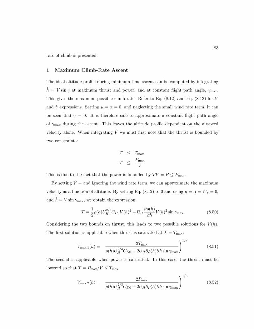
83
rate of climb is presented.
1 Maximum Climb-Rate Ascent
The ideal altitude profile during minimum time ascent can be computed by integrating
h = V sin γ at maximum thrust and power, and at constant flight path angle, γmax.
This gives the maximum possible climb rate. Refer to Eq. (8.12) and Eq. (8.13) for V
and γ expressions. Setting µ = α = 0, and neglecting the small wind rate term, it can
be seen that γ = 0. It is therefore safe to approximate a constant flight path angle
of γmax during the ascent. This leaves the altitude profile dependent on the airspeed
velocity alone. When integrating V we must first note that the thrust is bounded by
two constraints:
T ≤ Tmax
T ≤ Pmax
V
This is due to the fact that the power is bounded by TV = P ≤ Pmax.
By setting V = and ignoring the wind rate term, we can approximate the maximum
velocity as a function of altitude. By setting Eq. (8.12) to 0 and using µ = α = Wx = 0,
and h = V sin γmax, we obtain the expression:
T =1
2ρ(h)U
2/3H CD0V (h)2 + UH
∂ρ(h)
∂hV (h)2 sin γmax (8.50)
Considering the two bounds on thrust, this leads to two possible solutions for V (h).
The first solution is applicable when thrust is saturated at T = Tmax:
Vmax,1(h) =
(2Tmax
ρ(h)U2/3H CD0 + 2UH∂ρ(h)∂h sin γmax
)1/2
(8.51)
The second is applicable when power is saturated. In this case, the thrust must be
lowered so that T = Pmax/V ≤ Tmax.
Vmax,2(h) =
(2Pmax
ρ(h)U2/3H CD0 + 2UH∂ρ(h)∂h sin γmax
)1/3
(8.52)
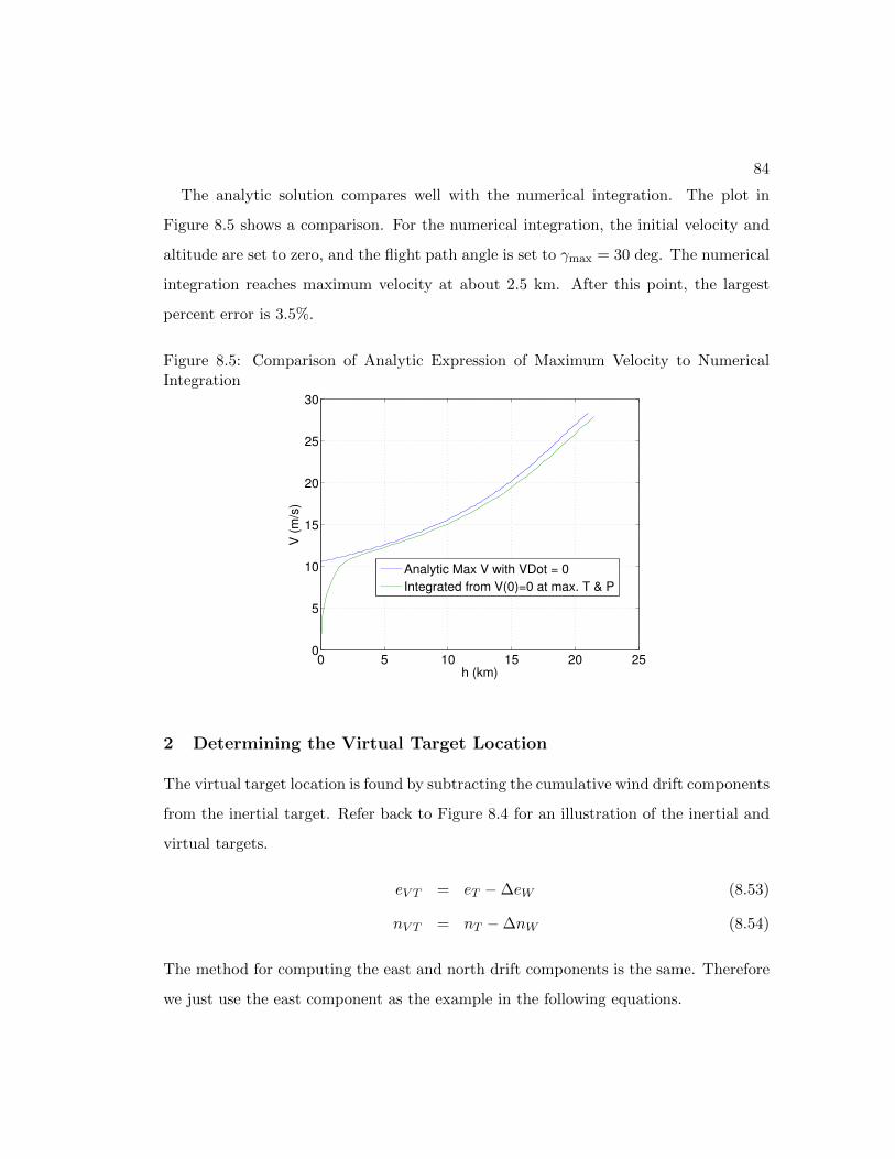
84
The analytic solution compares well with the numerical integration. The plot in
Figure 8.5 shows a comparison. For the numerical integration, the initial velocity and
altitude are set to zero, and the flight path angle is set to γmax = 30 deg. The numerical
integration reaches maximum velocity at about 2.5 km. After this point, the largest
percent error is 3.5%.
Figure 8.5: Comparison of Analytic Expression of Maximum Velocity to NumericalIntegration
0 5 10 15 20 250
5
10
15
20
25
30
h (km)
V (
m/s
)
Analytic Max V with VDot = 0
Integrated from V(0)=0 at max. T & P
2 Determining the Virtual Target Location
The virtual target location is found by subtracting the cumulative wind drift components
from the inertial target. Refer back to Figure 8.4 for an illustration of the inertial and
virtual targets.
eV T = eT −∆eW (8.53)
nV T = nT −∆nW (8.54)
The method for computing the east and north drift components is the same. Therefore
we just use the east component as the example in the following equations.

85
As the airship ascends in the wind-relative frame, the Eastward and Northward wind
speeds change. The integration of the wind in each direction over time determines the
total amount of drift due to the wind.
∆eW =
∫ tF
t0
WE(t)dt (8.55)
Our model for the wind is a function of altitude, however, and so we must introduce
a change of variable. The general formula for integration with a substitution of variable
from t to x is: ∫ g(b)
g(a)f(t)dt =
∫ b
af(g(x))g′(x)dx (8.56)
where t = g(x). In our problem, we wish to change the integration variable from time
t to altitude h. The original function to integrate is f(t) = WE(t) and the time is
expressed as a function of altitude, t = g(h). Therefore, we have:∫ tF
t0
WE(t)dt =
∫ hF
h0
WE(g(h))g′(h)dh (8.57)
In order to find the functional form for t = g(h), we begin with the equation for the
altitude rate:dh
dτ= V (h) sin γ (8.58)
In this derivation we assume that γ is constant, which is true for each segment of the
assumed optimal solution structure used in planning minimum-time flights. Rearranging
Eq. 8.58 to isolate dh and dτ on each side, we have:(
1
sin γ
)dh
V (h)= dτ (8.59)
Integrating from t0 to time t, we have:
t− t0 =
∫ t
t0
dτ =1
sin γ
∫ hF
h0
dh
V (h)(8.60)
For a fixed γ and a known velocity profile, this gives the expected time to climb.
The resulting expression for the cumulative wind drift is:
∆eW =
∫ tF
t0
WE(t)dt =1
sin γ
∫ hF
h0
WE(h)
V (h)dh (8.61)

86
For the minimum-time profile, we use γ = γmax and a maximum velocity profile. The
maximum velocity formula of Eqs. 8.51 and 8.52 can be used to give a purely analytic
expression that can be integrated to give a closed-form solution. A further simplifying
step would be to compute a polynomial fit in h for 1/Vmax(h). Multiplied with the
polynomial of WE(h), this would simply give a higher order polynomial whose integral
can be found easily. Implementing this latter approach enables the cumulative wind
drift to be evaluated with minimal computational effort. This is particularly important
if the evaluation must be done repeatedly in an optimization.
With ∆eW and ∆nW computed, the horizontal distance to the virtual target dH can
be computed with Eq. (8.48), and the ascent cone radius RT is found from Eq. (8.48). If
dH ≤ Rc, this then the virtual target is inside the ascent cone; otherwise it lies outside.
The optimal solution for each case is described in the sections below.
3 Virtual Target Inside the Ascent Cone, dH ≤ Rc
We first consider the case where the virtual target is inside the ascent cone. An example
illustration is provided in Figure 8.6. The desired longitudinal motion to fly at max-
imum flight path angle, and at maximum thrust and power, until the target altitude
is reached. Using this altitude profile, the integral effect of the wind can be computed
to determine the virtual target location. The airship must then vary the heading such
that it intercepts the virtual target at the end of the ascent.
There are in fact an infinite number of ways to vary the heading. As the objective
here is to minimize time of flight, the most direct approach is appropriate. One simple
and direct method is to fly at a constant turn rate along a circular arc, as projected in
the horizontal plane. Since the airship flies at maximum flight path angle, the horizontal
distance flown is equal to the ascent cone radius, Rc. Therefore, the virtual target is
intercepted if the arc length s (along the circle to the virtual target) is equal to the
ascent cone radius Rc.
An illustration of the turning radius geometry is shown in Figure 8.7. The direction
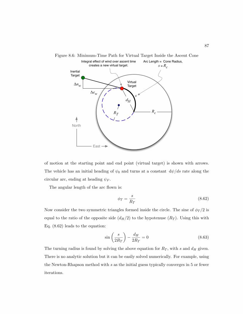
87
Figure 8.6: Minimum-Time Path for Virtual Target Inside the Ascent Cone
VirtualTarget
InertialTarget
Arc Length = Cone Radius, s = Rc
s
Rc
dH
RT
Integral effect of wind over ascent time creates a new virtual target.
ΔnwΔew
North
East
of motion at the starting point and end point (virtual target) is shown with arrows.
The vehicle has an initial heading of ψ0 and turns at a constant dψ/ds rate along the
circular arc, ending at heading ψF .
The angular length of the arc flown is:
φT =s
RT(8.62)
Now consider the two symmetric triangles formed inside the circle. The sine of φT /2 is
equal to the ratio of the opposite side (dH/2) to the hypotenuse (RT ). Using this with
Eq. (8.62) leads to the equation:
sin
(s
2RT
)− dH
2RT= 0 (8.63)
The turning radius is found by solving the above equation for RT , with s and dH given.
There is no analytic solution but it can be easily solved numerically. For example, using
the Newton-Rhapson method with s as the initial guess typically converges in 5 or fewer
iterations.

88
Figure 8.7: Constant Turning Radius for Virtual Target Inside the Ascent Cone
VirtualTarget
ψ0
RTStartingPoint
RT
dH2
s2
s2
dH2
!T
s = Rc
"
ψF
Also, note that for the limiting case of dH = s, the solution is RT = ∞, which
corresponds to a straight line. This is consistent with the definition of the ascent cone.
The heading rate is derived by first applying the chain rule to get:
dψ
ds=dψ
ds
ds
dt(8.64)
The first term dψ/ds is the rate of change of heading with respect to the arc length. Be-
cause a circular arc is flown, this is a constant equal to the inverse of the turning radius,
1/RT . The second term ds/dt is the horizontal velocity, which is V cos γ. Therefore,
the heading angle history can be expressed as:
ψ(t) = ψ0 +1
RT
∫ t
0V (τ) cos γmaxdτ (8.65)
where the initial heading is determined from the geometry to be:
ψ0 =
β ± φ/2 s ≤ πRTβ ± φ/2 + π s > πRT
(8.66)

89
and β is the angle from the starting point to the target, measured from north.
tanβ =∆e
∆n(8.67)
The sign on the (φ/2) term in each case is arbitrary. This is due to the fact that the
diagram could have been drawn differently, reversing it about the dH line (from starting
point to virtual target). In that case the arc length would have been the same but the
initial heading would be towards the east rather than the northwest.
Two examples of the turn radius calculation are shown below. In both cases, the
ascent cone radius is Rc = 10 km. In the plot on the left, the virtual target is at
coordinates (1, 2) km in the East-North plane. The solution to Eq. (8.63) yields RT =
1.97 km. Computing the turn angle with Eq. (8.62) gives φ = 5.07 rad. In the right-
hand side plot, the virtual target is moved to coordinates (5, 6) km, and the turn radius
is RT = 4.2 km with a turn angle of φ = 2.37 rad.
Figure 8.8: Constant Turn Radius Examples
−10 −5 0 5 10
−8
−6
−4
−2
0
2
4
6
8
AscentConeRadius
East (km)
Nort
h (
km
)
Constant Turn Radius, s > π RT
AscentConeRadius
−10 −5 0 5 10
−8
−6
−4
−2
0
2
4
6
8
AscentConeRadius
East (km)
Nort
h (
km
)
Constant Turn Radius, s < π RT
AscentConeRadius
Example of Minimum-Time Plan with Virtual Target Inside the Ascent Cone
Here, an example of a minimum-time ascent plan is presented where the virtual target
is inside the ascent cone. We use one of the cases from Scenario 4, where the target
station is 10 km east of the launch site, and the target altitude is again 21 km. The
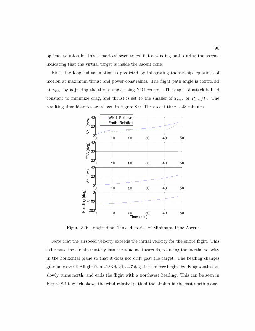
90
optimal solution for this scenario showed to exhibit a winding path during the ascent,
indicating that the virtual target is inside the ascent cone.
First, the longitudinal motion is predicted by integrating the airship equations of
motion at maximum thrust and power constraints. The flight path angle is controlled
at γmax by adjusting the thrust angle using NDI control. The angle of attack is held
constant to minimize drag, and thrust is set to the smaller of Tmax or Pmax/V . The
resulting time histories are shown in Figure 8.9. The ascent time is 48 minutes.
0 10 20 30 40 500
20
40
Vel. (
m/s
)
0 10 20 30 40 5020
30
40
FP
A (
deg)
0 10 20 30 40 500
20
40
Alt. (k
m)
0 10 20 30 40 50−200
−100
0
Headin
g (
deg)
Time (min)
Wind−Relative
Earth−Relative
Figure 8.9: Longitudinal Time Histories of Minimum-Time Ascent
Note that the airspeed velocity exceeds the initial velocity for the entire flight. This
is because the airship must fly into the wind as it ascends, reducing the inertial velocity
in the horizontal plane so that it does not drift past the target. The heading changes
gradually over the flight from -133 deg to -47 deg. It therefore begins by flying southwest,
slowly turns north, and ends the flight with a northwest heading. This can be seen in
Figure 8.10, which shows the wind-relative path of the airship in the east-north plane.
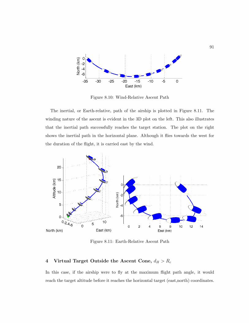
91
Figure 8.10: Wind-Relative Ascent Path
The inertial, or Earth-relative, path of the airship is plotted in Figure 8.11. The
winding nature of the ascent is evident in the 3D plot on the left. This also illustrates
that the inertial path successfully reaches the target station. The plot on the right
shows the inertial path in the horizontal plane. Although it flies towards the west for
the duration of the flight, it is carried east by the wind.
Figure 8.11: Earth-Relative Ascent Path
4 Virtual Target Outside the Ascent Cone, dH > Rc
In this case, if the airship were to fly at the maximum flight path angle, it would
reach the target altitude before it reaches the horizontal target (east,north) coordinates.

92
Therefore, it must fly for some portion of the trajectory at a lower flight path angle. This
is evidenced in the optimal trajectories presented in Chapter 6. For example, Figure 6.1
shows the minimum-time ascent from 250 km downrange flying for a significant portion
at 14 km, to make use of the peak east winds at that altitude.
The general structure of optimal solution for this case is as follows:
1. Ascend at the maximum climb-rate to cruise altitude hC
• Heading: ψA
• Velocity: Vmax(h)
• Flight path angle: γmax
2. Fly at cruise altitude hC for time duration ∆tC
• Heading: ψC
• Velocity: Vmax(hC)
• Flight path angle: 0
3. Ascend (or descend) at the maximum climb-rate to target altitude hT
• Heading: ψA
• Velocity: Vmax(h)
• Flight path angle: ±γmax
The approach taken here is to build a trajectory according to this structure in order
to emulate the optimal minimum-time ascent solution. The set of parameters describing
the trajectory include: ascent heading ψA, the cruise altitude hC , cruise heading ψC
and cruise time ∆tC . Thus, the size of the problem is reduced to just a few decision
variables. The full problem formulation with objective function and constraints will be
presented below.

93
First, the overall geometry is described in Figure 8.12. Here, the ascent heading has
been intentionally drawn as ψA = 0 to simplify the diagram for visual clarity. As shown,
the airship first ascends at the maximum flight path, with a fixed ascent heading. It
then flies at a constant altitude at some other coast heading, and finally ascends to the
target altitude at the ascent heading. All segments are flown at maximum airspeed,
with thrust and/or power at their limit.
Figure 8.12: Minimum-Time Path for Virtual Target Inside the Ascent Cone
!max , ψA= 0
ψC
!max , ψA= 0
North
East
Up (Wind-Relative)VirtualTarget
Rc
dH
hT
North
East
hC
hT - hC
The total time to reach the station is approximated as the ascent time plus the
horizontal cruise time:
tF ≈ ∆tA + ∆tC (8.68)
The duration of the ascent phase is already minimized, as it is flown at the maximum
rate of climb. Therefore, the task of minimizing the total ascent time for this trajectory
reduces to a minimization of the cruise time.
To develop an expression for the cruise time, first consider the details of the ascent
structure, as illustrated in Figure 8.13. The airship starts at the center of the ascent
cone with radius Rc. It ascends at heading ψA to reach coordinates (eA0, nA0) at the
end of the ascent phase. This position is marked with a bold blue circle on the ascent
cone perimeter. During this time, the wind velocity produces a cumulative drift of ∆ew
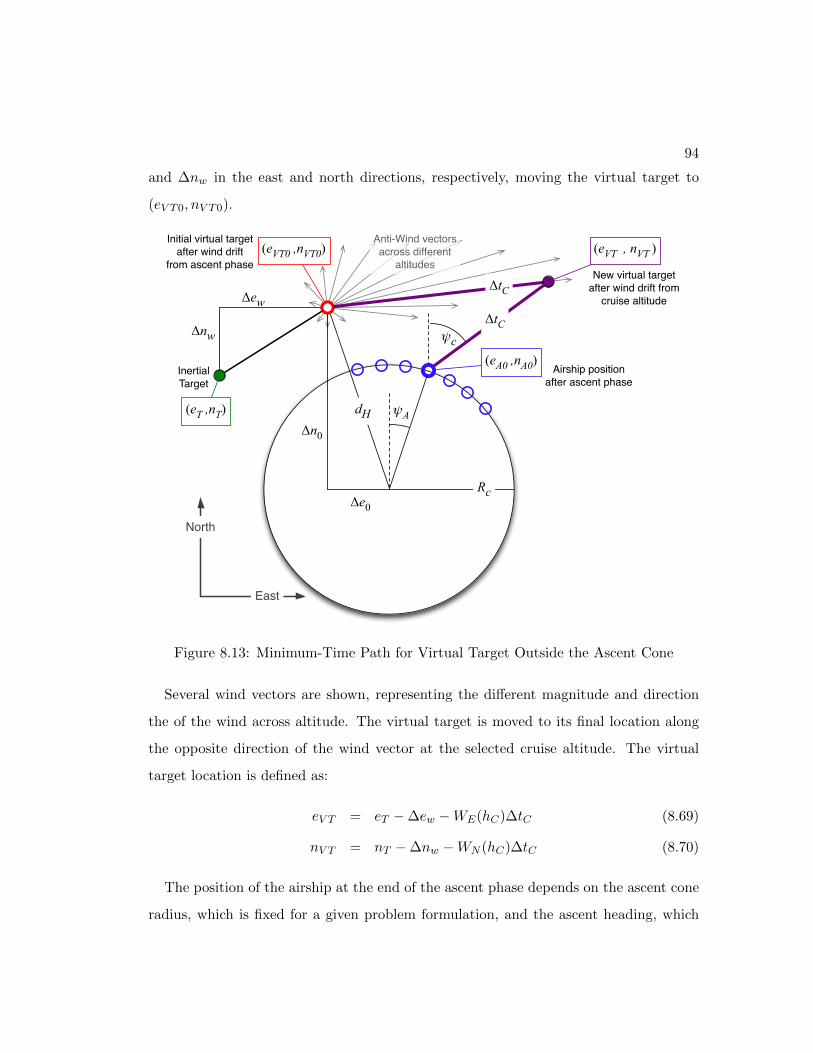
94
and ∆nw in the east and north directions, respectively, moving the virtual target to
(eV T0, nV T0).
ψc
New virtual targetafter wind drift from
cruise altitude
InertialTarget
Rc
dH
Δnw
ΔewΔtC
ΔtC
Anti-Wind vectorsacross different
altitudes(eVT0 ,nVT0)
North
East
ψA
Δe0
Δn0
Initial virtual targetafter wind drift
from ascent phase(eVT , nVT )
(eT ,nT)
Airship positionafter ascent phase
(eA0 ,nA0)
Figure 8.13: Minimum-Time Path for Virtual Target Outside the Ascent Cone
Several wind vectors are shown, representing the different magnitude and direction
the of the wind across altitude. The virtual target is moved to its final location along
the opposite direction of the wind vector at the selected cruise altitude. The virtual
target location is defined as:
eV T = eT −∆ew −WE(hC)∆tC (8.69)
nV T = nT −∆nw −WN (hC)∆tC (8.70)
The position of the airship at the end of the ascent phase depends on the ascent cone
radius, which is fixed for a given problem formulation, and the ascent heading, which
95
may be varied. The coordinates are:
eA0 = Rc sinψA (8.71)
nA0 = Rc cosψA (8.72)
In order to reach the virtual target, the airship must fly at the required heading ψC .
At the given cruise altitude, it has maximum velocity Vmax(hC). Therefore, the equation
for the east position at the end of the cruise phase is:
eA0 + Vmax(hC) sinψC∆tC = eT −∆ew −WE(hC)∆tC (8.73)
Rearranging to solve for ∆tC gives:
∆tC =eT −∆ew −Rc sinψA
Vmax(hC) sinψC +WE(hC)(8.74)
Using the north component produces a similar equation:
∆tC =nT −∆nw −Rc cosψA
Vmax(hC) cosψC +WN (hC)(8.75)
Setting Eq. (8.74) and Eq. (8.75) equal enables ψC to be isolated in a function with the
inertial target coordinates, the wind drift components, the wind velocities and maximum
airspeed velocity at hC , and the ascent heading ψA.
(Vmax(hC) cosψC +WN (hC)) (eT −∆ew −Rc sinψA) = (8.76)
(Vmax(hC) sinψC +WE(hC)) (nT −∆nw −Rc cosψA)
This can be solved for sinψC by isolating its cosine and sine terms, setting sinψC =
±√
1− cos2 ψC , and squaring both sides of the equation. This leads to a quadratic
expression in sinψC which is readily solved.
Thus far, we have developed an equation for the cruise time ∆tC as a function of
given parameters (eV T0, Rc), and the variables ψA, hC , and ψC . We have further found
that ψC can be solved explicitly as a function of hC , ψA. We are now in a position to

96
minimize the cruise time over the variables hC , ψA. First, however, we must consider
the constraints on the inertial heading during the cruise phase.
One unique characteristic of airships that is not found in traditional aircraft is that
they often fly at an airspeed that is slower than the ambient wind. As a simple example,
consider an airship flying with a wind-relative speed of V = 10 m/s towards the west,
but the wind is blowing east at WE = 25 m/s. The inertial motion of the vehicle would
of course be towards the east at VI = 15 m/s. In this case, it would not be possible
for the airship attain an inertial velocity towards the west, due to the overpowering
influence of the wind. This potential limitation on inertial heading must be considered
when selecting a cruse altitude.
When the cruise altitude is selected, it defines the wind magnitudeW =√W 2E(hC) +W 2
N (hC)
and direction ψW = tan−1(WE/WN ), as well as the airspeed velocity V = Vmax(hC).
The diagram in Figure 8.14 illustrates the inertial heading constraints for the case when
the wind magnitude is greater than the airspeed, W > V .
The inertial velocity is shown as the vector sum of the wind velocity and the airship’s
wind-relative velocity. A circle of radius V is drawn at the tip of the wind vector,
indicating that the vehicle can fly in any wind-relative direction. However, since the
wind velocity magnitude, which is not controllable, is greater than the ship’s airspeed,
this limits the achievable heading range for the inertial velocity. The attainable range
of inertial velocity directions is marked with blue lines. As the geometry shows, the
limits are:
ψI,min = ψW −∆θ (8.77)
ψI,max = ψW + ∆θ (8.78)
where the angle ∆θ is found to be
∆θ = sin−1
(V
W
)
Consider again the geometry of the cruise phase in Figure 8.13. The east distance to
the target is eV T0 − eA0, and the north distance is nV T0 − nA0. The inertial heading

97
Targets can be reached
in this region
Heading Range for Inertial Velocity
!θ
ψW
Targets cannot be reached
in this regionNorth
East
V
VI
W
Figure 8.14: Heading Constraint for Minimum-Time Ascent

98
angle is therefore:
ψI = tan−1
(eV T0 − eA0
nV T0 − nA0
)
If it is the case that W > V , then in order for the airship to be capable of reaching the
target, this heading angle must lie within the inertial heading limits described above:
ψI,min ≤ ψI ≤ ψI,max. Expanding each term, the constraints are written as a function
of the given parameters and variables hC , ψA as follows:
tan−1
(eV T0 −Rc sinψAnV T0 − nA0
)≥ tan−1
(WE(hC)
WN (hC)
)− sin−1
Vmax(hC)√
W 2E(hC) +W 2
N (hC)
(8.79)
tan−1
(eV T0 −Rc sinψAnV T0 − nA0
)≤ tan−1
(WE(hC)
WN (hC)
)+ sin−1
Vmax(hC)√
W 2E(hC) +W 2
N (hC)
(8.80)
With the cost function and the constraints now fully developed, we may write the com-
plete problem formulation. The problem again is to minimize the cruise time through
selection of the cruise altitude hC and ascent heading ψA, subject to constraints on the
inertial cruise heading. The minimum-time problem formulation is:
Minimum-Time Problem Formulation - Outside Ascent Cone, dH > Rc
minhC ,ψA
∆tC =eV T0 −Rc sinψA
Vmax(hC) sinψC +WE(hC)(8.81)
s.t. tan−1
(eV T0 −Rc sinψAnV T0 −Rc cosψA
)− tan−1
(WE(hC)
WN (hC)
)− sin−1
(Vmax(hC)
W (hC)
)≤ 0
− tan−1
(eV T0 −Rc sinψAnV T0 −Rc cosψA
)+ tan−1
(WE(hC)
WN (hC)
)− sin−1
(Vmax(hC)
W (hC)
)≤ 0
where the cruise heading is solved explicitly according to the equation:
Vmax(hC)∆e(ψA) cosψC−Vmax(hC)∆n(ψA) sinψC +WN (hC)∆e(ψA)−WE∆n(ψA) = 0
and the following abbreviations have been used:
W (hC) =√W 2E(hC) +W 2
N (hC)
∆e(ψA) = eV T0 −Rc sinψA
∆n(ψA) = nV T0 −Rc cosψA
99
The above problem formulation is a nonlinear program with two variables and two
constraints. It is solved using Matlab’s fmincon program with the sequential quadratic
programming method (SQP). This approach computes a quasi-Newton approximation
to the Hessian of the Lagrangian through evaluation of the cost and constraint functions.
Whereas the original minimum-time optimization included thousands of variables
and constraints, taking tens to hundreds of seconds to reach a solution, this problem is
routinely solved in less than 0.25 seconds. 1
Example of Minimum-Time Plan with Virtual Target Outside the Ascent
Cone
Consider the minimum-time ascent of Scenario 2 from Figure 6.1. The same conditions
are repeated here and the solution is generated using the above alternative optimization
method. In this case, the virtual target is outside the ascent cone, requiring a substantial
cruise phase. A comparison of the original SNOPT solution and the new alternative
method are shown in Figure 8.15. The two profiles agree closely, with both following a
constant altitude cruise segment at about 14 km. The original SNOPT solution predicts
a minimum time of 2 hours and 1 minute, compared with the new method’s result of 2
hours and 5 minutes.
We now consider another example, where the target station is located 120 km east
and 20 km south of the launch site. The same east wind profile is used, and a north wind
profile is added that varies between -4 and +4 m/s. The total flight time is computed
across a range of possible cruise altitudes and ascent headings, and the result is plotted
with a color-map surface contour in Figure 8.16. The dark red region in the lower left
corner is infeasible, as the combination of ascent heading and cruise altitude here would
prevent the airship from overcoming the wind velocity. The color-map legend is shown
in units of minutes. This shows that, even with a poor initial guess, the optimization
method converges to the verified optimal solution.
1 Mac PowerBook, Mac OS 10.7.5, 2 GHz Intel Core i7 processor, 4 GB RAM, Matlab R2013A
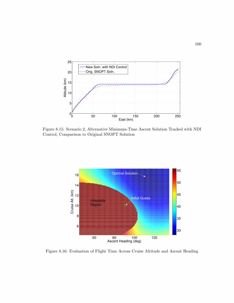
100
0 50 100 150 200 2500
5
10
15
20
25
East (km)
Altitu
de
(km
)
New Soln. with NDI Control
Orig. SNOPT Soln.
Figure 8.15: Scenario 2, Alternative Minimum-Time Ascent Solution Tracked with NDIControl, Comparison to Original SNOPT Solution
6
8
10
12
14
16
60 80 100 120
Ascent Heading (deg)
Cru
ise A
lt. (k
m)
30
35
40
45
50
55Optimal Solution
Initial GuessInfeasibleRegion
Figure 8.16: Evaluation of Flight Time Across Cruise Altitude and Ascent Heading
101
8.5 Minimum-Energy Ascent
In this section we develop new problem formulations involving trajectory models that
emulate the structure of known minimum-energy solutions, with the immediate goal of
reducing the computation time required to generate a solution. The ultimate objective
is to apply this technique to rapidly develop near minimum-energy ascent plans for
onboard implementation. A significant decrease in the planning computation time is
achieved by greatly reducing the number of decision variables, and quickly generating
an initial guess that is close to being feasible.
The minimum-energy solutions found from prior numerical optimization work indicate
two different basic structures of the optimal solution. One type of solution involves a
steady longitudinal ascent, at roughly constant airspeed and flight path angle, while the
wind-relative heading varies. The second type of solution involves a steady wind-relative
heading with three longitudinal segments: 1) a steepest ascent at roughly constant
airspeed to the maximum operational altitude, 2) a constant velocity, level flight towards
the station, and 3) a short descent to the station altitude.
The former structure, where the heading varies over time, is termed a winding ascent.
The latter, where the heading is nearly constant, is termed a direct ascent. The remain-
der of this section discusses the modeling of these trajectory structures, and presents
optimization methods to compute minimum energy trajectories that intercept the target
station.
The procedure for computing the minimum-energy ascent plan is summarized in
Figure 8.17. The first step is to identify which of the ascent types, direct or winding,
should be used. To do this, we begin by computing a minimum energy solution for the
simplest possible ascent, which is a straight line to the virtual target at constant velocity.
If necessary, an additional cruise segment at constant altitude, constant velocity, may
also be used. This initial trajectory structure is termed the simple ascent. If a horizontal
cruise segment is used in the simple ascent, then we go on to compute a direct ascent

102
plan. Otherwise, if no horizontal segment is used, we compute a winding ascent plan.
ComputeSimple Ascent Plan
Compute Direct Ascent Plan
HorizontalSegmentNeeded?
ComputeWinding Ascent Plan
GenerateInitial Guess
for Winding Ascent
GenerateInitial Guess
for Direct AscentYes
No
Figure 8.17: Procedure for Developing Minimum-Energy Ascent Plan
Each of the aforementioned methods is presented in the sections that follow. First,
however, it is necessary to establish the fundamental components of the trajectory model
that are used to develop each ascent profile.
Longitudinal Motion with Piecewise Linear Segments of V, γ
Let us now model the trajectory of the airship as a series of segments where its airspeed
and flight path angle change linearly with time. Thus, over a time increment 0 ≤ t ≤∆Tk from point k to k + 1 in the segment, we have:
V (t) = Vk + at (8.82)
γ(t) = γk + bt (8.83)
where a and b give the constant rate of change in velocity and flight path angle, respec-
tively, over the segment. These are defined as follows:
a = (Vk+1 − Vk) /∆Tk (8.84)
b = (γk+1 − γk) /∆Tk (8.85)
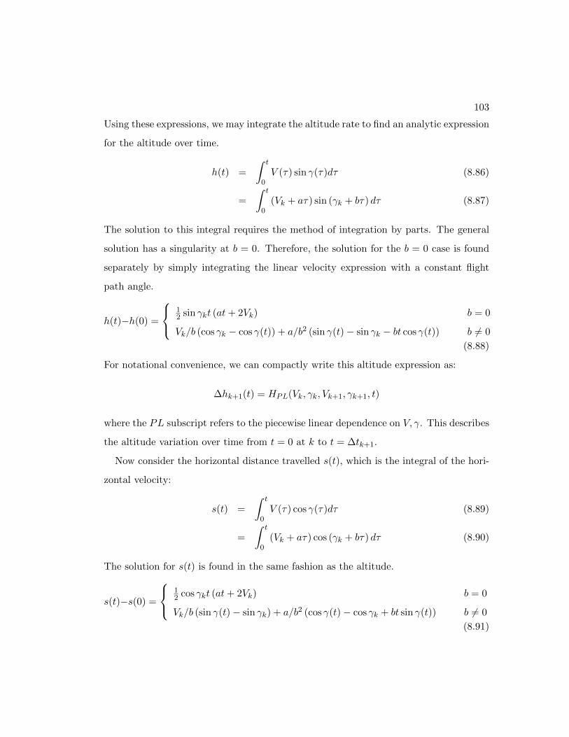
103
Using these expressions, we may integrate the altitude rate to find an analytic expression
for the altitude over time.
h(t) =
∫ t
0V (τ) sin γ(τ)dτ (8.86)
=
∫ t
0(Vk + aτ) sin (γk + bτ) dτ (8.87)
The solution to this integral requires the method of integration by parts. The general
solution has a singularity at b = 0. Therefore, the solution for the b = 0 case is found
separately by simply integrating the linear velocity expression with a constant flight
path angle.
h(t)−h(0) =
12 sin γkt (at+ 2Vk) b = 0
Vk/b (cos γk − cos γ(t)) + a/b2 (sin γ(t)− sin γk − bt cos γ(t)) b 6= 0
(8.88)
For notational convenience, we can compactly write this altitude expression as:
∆hk+1(t) = HPL(Vk, γk, Vk+1, γk+1, t)
where the PL subscript refers to the piecewise linear dependence on V, γ. This describes
the altitude variation over time from t = 0 at k to t = ∆tk+1.
Now consider the horizontal distance travelled s(t), which is the integral of the hori-
zontal velocity:
s(t) =
∫ t
0V (τ) cos γ(τ)dτ (8.89)
=
∫ t
0(Vk + aτ) cos (γk + bτ) dτ (8.90)
The solution for s(t) is found in the same fashion as the altitude.
s(t)−s(0) =
12 cos γkt (at+ 2Vk) b = 0
Vk/b (sin γ(t)− sin γk) + a/b2 (cos γ(t)− cos γk + bt sin γ(t)) b 6= 0
(8.91)
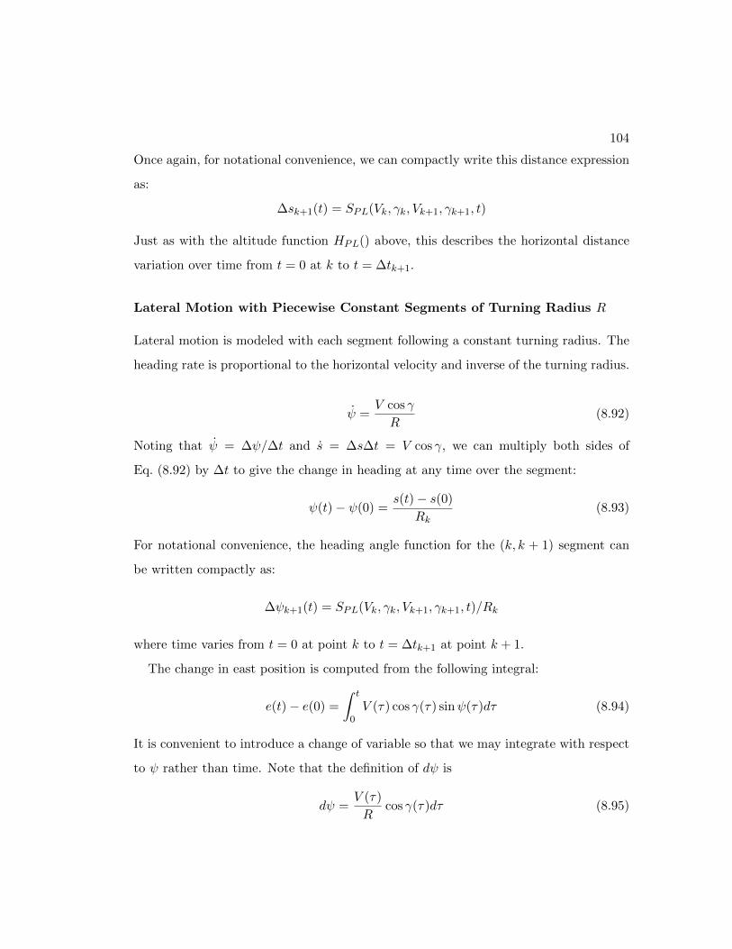
104
Once again, for notational convenience, we can compactly write this distance expression
as:
∆sk+1(t) = SPL(Vk, γk, Vk+1, γk+1, t)
Just as with the altitude function HPL() above, this describes the horizontal distance
variation over time from t = 0 at k to t = ∆tk+1.
Lateral Motion with Piecewise Constant Segments of Turning Radius R
Lateral motion is modeled with each segment following a constant turning radius. The
heading rate is proportional to the horizontal velocity and inverse of the turning radius.
ψ =V cos γ
R(8.92)
Noting that ψ = ∆ψ/∆t and s = ∆s∆t = V cos γ, we can multiply both sides of
Eq. (8.92) by ∆t to give the change in heading at any time over the segment:
ψ(t)− ψ(0) =s(t)− s(0)
Rk(8.93)
For notational convenience, the heading angle function for the (k, k + 1) segment can
be written compactly as:
∆ψk+1(t) = SPL(Vk, γk, Vk+1, γk+1, t)/Rk
where time varies from t = 0 at point k to t = ∆tk+1 at point k + 1.
The change in east position is computed from the following integral:
e(t)− e(0) =
∫ t
0V (τ) cos γ(τ) sinψ(τ)dτ (8.94)
It is convenient to introduce a change of variable so that we may integrate with respect
to ψ rather than time. Note that the definition of dψ is
dψ =V (τ)
Rcos γ(τ)dτ (8.95)

105
Substituting this into Eq. (8.94) we have:
e(t)− e(0) = Rk
∫ ψ(t)
ψ(0)sinψdψ (8.96)
= Rk (cosψ(0)− cosψ(t)) (8.97)
Similarly, the north position is computed from the integral:
n(t)− n(0) =
∫ t
0V (τ) cos γ(τ) cosψ(τ)dτ (8.98)
Again, substitution is used to express the integral as a function of ψ, giving:
n(t)− n(0) = Rk
∫ ψ(t)
ψ(0)cosψdψ (8.99)
= Rk (sinψ(t)− sinψ(0)) (8.100)
1 Minimum-Energy Simple Ascent Profile
The cumulative energy is the integral of the applied power over time. With a propeller,
the required power is modeled as P = ηTV . In the simple ascent, we assume constant
velocity flight. Thus, thrust equals drag and so P = ηDV . Therefore, the energy is
expressed as:
E = η
∫ t
0D(h(τ))V dτ (8.101)
assuming constant efficiency across altitude, where τ is the integration variable for time.
We can introduce a change of variable by noting that h = dh/dτ , and instead integrate
across altitude. Define the limits of integration as h = h0 at τ = 0 and h = hF at τ = t.
Using the formula for drag, Eq. (8.101) becomes:
E =1
h
∫ hF
h0
1
2ρ(h)V 2SCDV dh (8.102)
=SCDV
3
2h
∫ hF
h0
ρ(h)dh
=SCDV
2
2 sin γρ(h0, hF ) (8.103)

106
where the notation X(a, b) is used to indicate the integration of the polynomial func-
tion X from limits a to b.
The simple ascent profile is modeled as a constant velocity and constant flight path
angle ascent, as above, with an optional horizontal cruise segment. The full problem
formulation for the minimum-energy simple ascent profile is given below. The energy
cost includes the energy consumed during both the ascent and the horizontal cruise
segment.
Minimum-Energy Problem Formulation - Simple Ascent
minV,γ,hC ,VC ,∆tC
E =1
2SCD
(V 2
2 sin γρ(h0, hF ) + ρ(hC)V 3
C∆tC
)(8.104)
s.t. ∆e2 + ∆n2 −∆x2 ≤ 0
∆e = eT −WE(h0, hF )
V sin γ−WE(hC)∆tC − e0
∆n = nT −WN (h0, hF )
V sin γ−WN (hC)∆tC − n0
∆x = (hT − h0)/ tan γ + VC∆tC
Here, ∆x is the total horizontal distance covered during the combined ascent and
cruise segment. The inequality constraint ∆e2 + ∆n2 − ∆x2 ≤ 0 simply forces this
distance to exceed the horizontal distance to the virtual target, ensuring that the target
is reachable. If it is possible to satisfy this constraint with no cruise segment (∆tC = 0),
then this approach is favored as it would reduce the total energy.
It is interesting to note that the first energy term is inversely proportional to sin γ,
indicating that it is best to climb at the maximum flight path angle. This is intuitive,
as climbing at a shallower angle would tend to prolong the flight and lead to increased
energy usage. This is also consistent with the findings from extensive numerical opti-
mizations.
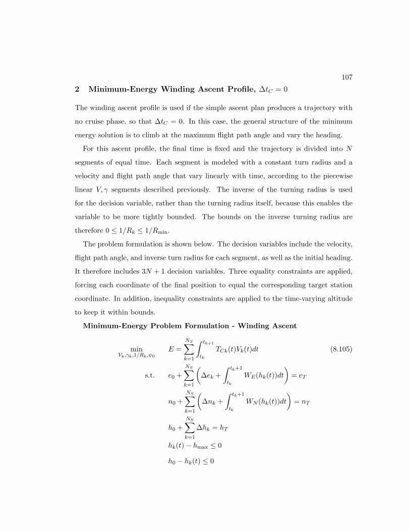
107
2 Minimum-Energy Winding Ascent Profile, ∆tC = 0
The winding ascent profile is used if the simple ascent plan produces a trajectory with
no cruise phase, so that ∆tC = 0. In this case, the general structure of the minimum
energy solution is to climb at the maximum flight path angle and vary the heading.
For this ascent profile, the final time is fixed and the trajectory is divided into N
segments of equal time. Each segment is modeled with a constant turn radius and a
velocity and flight path angle that vary linearly with time, according to the piecewise
linear V, γ segments described previously. The inverse of the turning radius is used
for the decision variable, rather than the turning radius itself, because this enables the
variable to be more tightly bounded. The bounds on the inverse turning radius are
therefore 0 ≤ 1/Rk ≤ 1/Rmin.
The problem formulation is shown below. The decision variables include the velocity,
flight path angle, and inverse turn radius for each segment, as well as the initial heading.
It therefore includes 3N + 1 decision variables. Three equality constraints are applied,
forcing each coordinate of the final position to equal the corresponding target station
coordinate. In addition, inequality constraints are applied to the time-varying altitude
to keep it within bounds.
Minimum-Energy Problem Formulation - Winding Ascent
minVk,γk,1/Rk,ψ0
E =
NS∑
k=1
∫ tk+1
tk
TCk(t)Vk(t)dt (8.105)
s.t. e0 +
NS∑
k=1
(∆ek +
∫ tk+1
tk
WE(hk(t))dt
)= eT
n0 +
NS∑
k=1
(∆nk +
∫ tk+1
tk
WN (hk(t))dt
)= nT
h0 +
NS∑
k=1
∆hk = hT
hk(t)− hmax ≤ 0
h0 − hk(t) ≤ 0

108
where the piecewise linear segments for velocity and flight path angle are:
Vk(t) = Vk−1 + (Vk − Vk−1)t− tk−1
tk − tk−1(8.106)
γk(t) = γk−1 + (γk − γk−1)t− tk−1
tk − tk−1(8.107)
The change in altitude, horizontal distance, and heading over each segment is:
∆hk(t) = HPL(Vk−1, γk−1, Vk, γk, t) (8.108)
∆sk(t) = SPL(Vk−1, γk−1, Vk, γk, t) (8.109)
∆ψk(t) = ∆sk(t)/Rk (8.110)
These are used to determine the altitude and heading over time:
hk(t) = h0 +
k∑
j=1
∆hk(t)
ψk(t) = ψ0 +
k∑
j=1
∆ψk(t)
(8.111)
Example Solutions
Consider the minimum-energy ascent for Scenario 2 in Figure 6.1, where the airship
starts its ascent 250 km west of the target station. The same conditions for this scenario
are repeated here and an alternative solution is generated using the winding ascent
optimization described above.
A simple ascent plan is computed first. Ten different solutions are generated using
random initial guesses and the lowest cost solution is chosen. In this scenario, all 10
solutions converge to the same structure, which has an approximate energy cost of
2.4 kW-hrs and a flight time of 4.8 hours. It takes 0.8 seconds to compute all 10
solutions.
Because the simple ascent solution has no cruise phase, a winding ascent plan is
computed. The results of the simple ascent trajectory are used to seed the initial guess
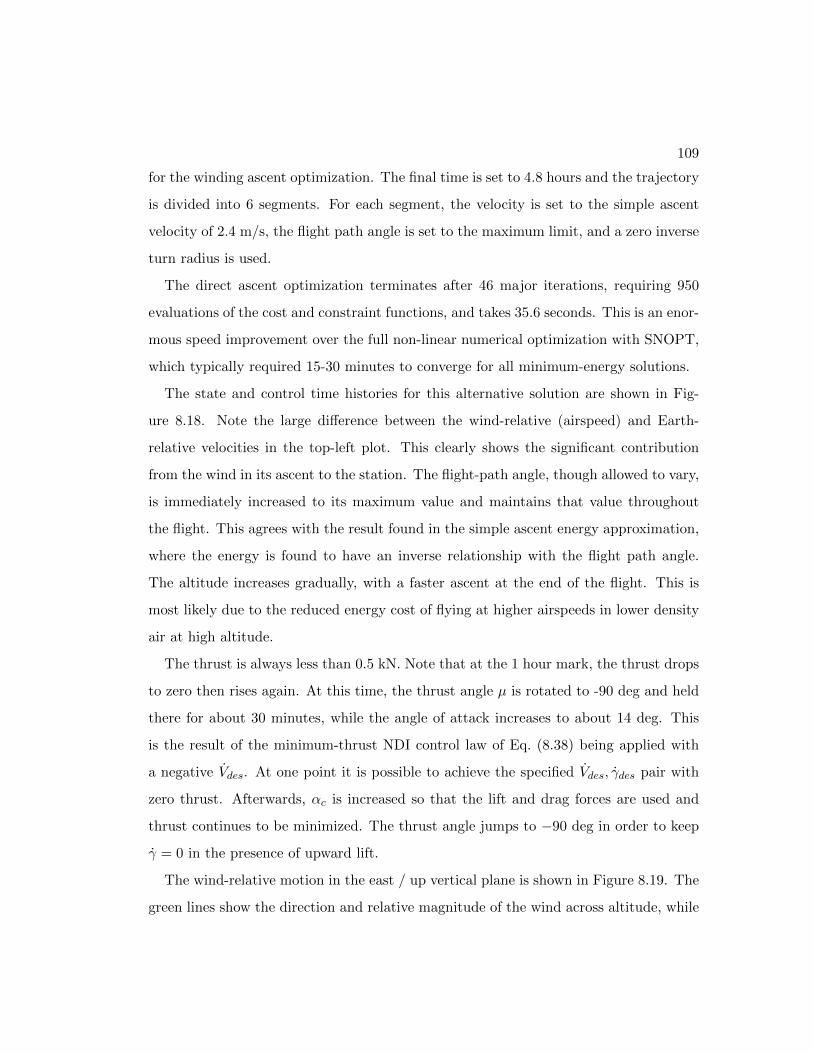
109
for the winding ascent optimization. The final time is set to 4.8 hours and the trajectory
is divided into 6 segments. For each segment, the velocity is set to the simple ascent
velocity of 2.4 m/s, the flight path angle is set to the maximum limit, and a zero inverse
turn radius is used.
The direct ascent optimization terminates after 46 major iterations, requiring 950
evaluations of the cost and constraint functions, and takes 35.6 seconds. This is an enor-
mous speed improvement over the full non-linear numerical optimization with SNOPT,
which typically required 15-30 minutes to converge for all minimum-energy solutions.
The state and control time histories for this alternative solution are shown in Fig-
ure 8.18. Note the large difference between the wind-relative (airspeed) and Earth-
relative velocities in the top-left plot. This clearly shows the significant contribution
from the wind in its ascent to the station. The flight-path angle, though allowed to vary,
is immediately increased to its maximum value and maintains that value throughout
the flight. This agrees with the result found in the simple ascent energy approximation,
where the energy is found to have an inverse relationship with the flight path angle.
The altitude increases gradually, with a faster ascent at the end of the flight. This is
most likely due to the reduced energy cost of flying at higher airspeeds in lower density
air at high altitude.
The thrust is always less than 0.5 kN. Note that at the 1 hour mark, the thrust drops
to zero then rises again. At this time, the thrust angle µ is rotated to -90 deg and held
there for about 30 minutes, while the angle of attack increases to about 14 deg. This
is the result of the minimum-thrust NDI control law of Eq. (8.38) being applied with
a negative Vdes. At one point it is possible to achieve the specified Vdes, γdes pair with
zero thrust. Afterwards, αc is increased so that the lift and drag forces are used and
thrust continues to be minimized. The thrust angle jumps to −90 deg in order to keep
γ = 0 in the presence of upward lift.
The wind-relative motion in the east / up vertical plane is shown in Figure 8.19. The
green lines show the direction and relative magnitude of the wind across altitude, while
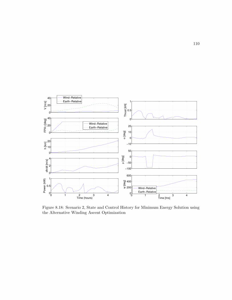
110
0
20
40
V [
m/s
]
Wind−Relative
Earth−Relative
0
20
40
FP
A γ
[deg]
Wind−Relative
Earth−Relative
0
10
20
h [km
]
0
2
4
dh/d
t [m
/s]
0 1 2 3 40
0.5
1
Pow
er
(kW
)
Time (hours)
0
0.5
1
Thru
st [k
N]
−10
0
10
20α
[deg]
−100
−50
0
50
µ [deg]
0 1 2 3 40
200
400
600
ψ [deg]
Time [hrs]
Wind−Relative
Earth−Relative
Figure 8.18: Scenario 2, State and Control History for Minimum Energy Solution usingthe Alternative Winding Ascent Optimization
111
the red lines show the airspeed velocity. Even though the airship travels 250 km to the
east, it only flies 5 km on its own, with the wind taking it the vast majority of the
distance.
−10 −5 0 5 100
5
10
15
20
25
East (km)
Altitu
de (
km
)
Figure 8.19: Scenario 2, Wind-Relative Motion in East / Up Plane
The wind-relative motion in the east / north horizontal plane is shown in Figure 8.20,
along with a time history of the turning radius inverse. The motion starts in the east
direction and turns south. The turn radius is at its smallest (highest 1/R) initially,
which can be seen in its path. The motion then approaches a straight line towards
the southwest with a large turn radius (low 1/R) before turning again north and east.
Finally, it flies in a nearly straight line towards the east to end the flight.
The cumulative energy over time is plotted in Figure 8.21, and the altitude vs. east
profile of the trajectory is plotted in Figure 8.22. The original solution from SNOPT is
shown for comparison in both plots. The close agreement in these plots clearly shows
that the alternative method is successfully finding a close approximation to the expected

112
−8 −6 −4 −2 0 2 4 6−12
−10
−8
−6
−4
−2
0
2
4
East (km)
Nort
h (
km
)
0 1 2 3 4 50
0.5
1
1.5
2
2.5
3
3.5
4
4.5x 10
−4
Time (hrs)
Invers
e o
f T
urn
ing R
adiu
s (
1/k
m)
Figure 8.20: Scenario 2, Wind-Relative Motion in East / North Plane
optimal solution.
0 0.5 1 1.5 2 2.5 3 3.5 4 4.5 50
0.2
0.4
0.6
0.8
1
1.2
1.4
Time (hrs)
Energ
y (
kW
−hrs
)
Winding Ascent Opt. Soln.
SNOPT Soln.
Figure 8.21: Scenario 2, Cumulative Energy History For the Winding Ascent Solution
3 Minimum-Energy Direct Ascent Profile, ∆tC > 0
The minimum energy solution for direct ascent may be approximated by constructing
a series of trajectory segments with constant V and γ. The trajectory consists of the

113
0 50 100 150 200 2500
5
10
15
20
25
East (km)
Altitude (
km
)
Winding Ascent Opt. Soln.
SNOPT Soln.
Figure 8.22: Scenario 2, Altitude vs. East Profile
following five segments:
Segment 0-1: Turn up to the maximum flight path angle.
Segment 1-2: Climb at the maximum flight path angle to a cruise altitude.
Segment 2-3: Turn down to zero flight path angle.
Segment 3-4: Cruise at constant altitude towards the target station.
Segment 4-5: Turn up/down to ascend/descend to the target altitude.
The diagram in Figure 8.23 describes the trajectory model. Variables shown in red
are decision variables for the optimization problem. All other variables are computed
implicitly. For some, the equations are simple enough to be shown in the diagram.
Others, shown with a surrounding box, are computed from the equations presented
below.
The total flight time is not fixed, but computed as the sum of each segment duration.
tF = ∆T1 + ∆T2 + ∆T3 + ∆T4 + ∆T5
For the first segment, we transition from (V0, h0, γ0) to (V1, h1, γ1) over a time interval
∆T1. With the initial conditions fixed, we select γ1 = γmax and solve for V1 as a function
of the parameters ∆T1, h1.

114
1
2
3 4
5
1-2 Ascend at maximum flight path angle.
0
Altitude
Wind-Relative Range
ΔT1Δh1
ΔT3 Δh3
h0V0γ0
0-1 Turn up to maximum flight path angle.
h1=h0+Δh1V1γ1=γmax
h2 = h3 - Δh3V2γ2 =γ1
2-3 Transition to level flight.
h3V3γ3=0
h4=h3V4=2 fAS |W|-V3
γ4=0h5 =hTV5γ5=+/- γmax
Given
ΔT2 Δh2= h2-h1
ΔT4 Δh4= 0 ΔT5
Δh5=h5 - h4
4-5 Descend to target altitude.
3-4 Level flight.
Figure 8.23: Profile of ascent trajectory with linear V, γ segments
b1 = (γ1 − γ0) /∆T1 (8.112)
a1 =b1 [(h1 − h0) b1 − V0 (cos γ0 − cos γ1)]
sin γ1 − sin γ0 − b1∆T1 cos γ1(8.113)
V1 = V0 + a1∆T1 (8.114)
In the next segment, we climb to condition (V2, h2, γ2). With a constant flight path
angle, b2 = 0 and the altitude equation is:
h2 = h1 +1
2∆T2 sin γ1 (V2 − V1) (8.115)
We can use Eq. (8.115) to compute the time interval ∆T2 in terms of h2 and V2:
∆T2 = 2h2 − h1
(V2 − V1) sin γ1(8.116)
Next, we compute the velocity V2 necessary to transition from (h2, γ2) to (V3, h3, γ3)
over the time interval ∆T3. Knowing that a3 = (V3−V2)/∆T3 and b3 = (γ3− γ2)/∆T3,

115
we can use Eq. (8.88) to solve for V2.
V2 = V3 −h3−h2∆T3
(γ3 − γ2)2 − V3(γ3 − γ2)(cos γ2 − cos γ3)
sin γ3 − sin γ2 − cos γ2(γ3 − γ2)(8.117)
From point 3 to 4 in the trajectory is a constant altitude cruise, so h4 = h3 and
γ3 = γ4 = 0. If the virtual target location before the cruise phase is already within the
horizontal distance, then no horizontal cruise segment is needed. The coordinates of
the virtual target before cruise are found by subtracting the east and north wind drift
from the first three flight segments.
∆e0,3 = eT −3∑
k=1
WE(hk−1, hk) (8.118)
∆n0,3 = nT −3∑
k=1
WN (hk−1, hk) (8.119)
Similarly, the wind-relative horizontal range ∆s0,3 traversed by the airship during these
segments is found by summing the range of each segment according to Eq. (8.91).
∆s0,3 =3∑
k=1
∆sPLVk−1, γk−1, Vk, γk) (8.120)
Again, if this range is greater than the distance to the virtual target, no horizontal
cruise segment is applied and the result is: ∆T4 = 0, V4 = V3. Otherwise, the airspeed
velocity at point 4 must be chosen to define the 3-4 flight segment. The average airspeed
for the 3-4 flight segment is:
V3,4 =1
2(V3 + V4)
Note that if the virtual target is in a direction opposite that of the wind velocity vector,
then the airspeed must exceed wind velocity magnitude in order to guarantee that the
target can be reached. We therefore set the average 3-4 flight segment velocity equal to
the wind velocity magnitude multiplied by an airspeed factor, fAS ≥ 0.
1
2(V3 + V4) = fAS
√W 2E(h4) +W 2
N (h4) (8.121)
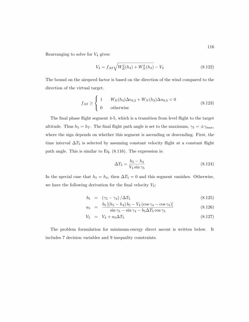
116
Rearranging to solve for V4 gives:
V4 = fAS
√W 2E(h4) +W 2
N (h4)− V3 (8.122)
The bound on the airspeed factor is based on the direction of the wind compared to the
direction of the virtual target.
fAS ≥
1 WE(h3)∆e0,3 +WN (h3)∆n0,3 < 0
0 otherwise(8.123)
The final phase flight segment 4-5, which is a transition from level flight to the target
altitude. Thus h5 = hT . The final flight path angle is set to the maximum, γ5 = ±γmax,
where the sign depends on whether this segment is ascending or descending. First, the
time interval ∆T5 is selected by assuming constant velocity flight at a constant flight
path angle. This is similar to Eq. (8.116). The expression is:
∆T5 =h5 − h4
V4 sin γ5(8.124)
In the special case that h5 = h4, then ∆T5 = 0 and this segment vanishes. Otherwise,
we have the following derivation for the final velocity V5:
b5 = (γ5 − γ4) /∆T5 (8.125)
a5 =b5 [(h5 − h4) b5 − V4 (cos γ4 − cos γ5)]
sin γ5 − sin γ4 − b5∆T5 cos γ5(8.126)
V5 = V4 + a5∆T5 (8.127)
The problem formulation for minimum-energy direct ascent is written below. It
includes 7 decision variables and 9 inequality constraints.

117
Minimum-Energy Problem Formulation - Direct Ascent, hC > 0
min∆t1,∆h1,∆t3,∆h3,h3,V3,fAS
E =5∑
k=1
∫ tk+1
tk
TCk(t)Vk(t)dt (8.128)
s.t. Vmin ≤ Vj ≤ Vmax ∀j ∈ 1, 2, 3, 4, 5
h1 = h0 + ∆h1
h2 = h3 −∆h3
h4 = h3
h5 = hT
∆e0 = eT −3∑
k=1
WE(hk−1, hk)
∆n0 = nT −3∑
k=1
WN (hk−1, hk)
fAS ≥
1 WE(h3)∆e0,3 +WN (h3)∆n0,3 < 0
0 otherwise
Example Solutions
Consider once again the minimum-energy ascent in Figure 6.1. This time we focus on
Scenario 1, where the airship starts its ascent 20 km east of the target station. The same
conditions for this scenario are repeated here and an alternative solution is generated
using the direct ascent optimization method described above.
A simple ascent plan is computed first. Ten different solutions are generated using
random initial guesses and the lowest cost solution is chosen. In this scenario, the best
approach is to cruise at the maximum operational altitude of 24 km. Typically 3-5
of the 10 solutions converge to this structure, which has an approximate energy cost
of 29 kW-hrs and a flight time of 18.4 hours. It takes 1.2 seconds to compute all 10
solutions.
The simple ascent plan has a cruise phase of 15.5 hours. Therefore, a direct ascent
plan is computed. The results of the simple ascent trajectory are used to seed the initial

118
guess for the direct ascent optimization. The cruise altitude was found to be h3 = hC =
24 km, the cruise velocity was V3 = VC = 6.68 m/s, and the climbing airspeed was
V = 4.94 m/s. The initial guess for transition times ∆T1,∆T3 are approximated as 5%
of the total flight time, and the altitude changes ∆h1,∆h3 are approximated with a
linear V, γ profile for those transition times and given boundary velocities.
The direct ascent optimization terminates after 25 major iterations, requiring 305
evaluations of the cost and constraint functions, and takes 34.1 seconds. This is compa-
rable with the winding ascent plan time. Once again, this provides a significant speed
improvement over the original, larger optimization problem that used SNOPT.
The state and control time histories for this alternative solution are shown in Fig-
ure 8.24. The wind-relative heading is fixed so that it flies directly towards the virtual
target, which in this case is due east. The thrust, thrust angle, and angle of attack
controls are computed according to the minimum thrust control policy with NDI inner-
loop control, according to Eq. (8.38). The velocity increases over the first two hours and
reaches a steady value of 6.8 m/s. The thrust and power vary over the first two hours
then remain fixed for the remainder of the flight, as the airship flies at constant velocity
at 24 km. This is consistent with the minimum-energy state and control history from
the original optimization using SNOPT.
The cumulative energy over time is plotted in Figure 8.25, and the altitude vs. east
profile of the trajectory is plotted in Figure 8.26. The original solution from SNOPT is
shown for comparison in both plots. Note that the original solution is for a 12 hour fixed
flight time, while the new solution lasts for 15.5 hours. Once again, the close agreement
in these plots indicates that the alternative optimization method is successfully finding
a good approximation to the expected optimal trajectory.

119
0
10
20
V [m
/s]
Wind−Relative
Earth−Relative
−100
0
100
FP
A γ
[deg]
Wind−Relative
Earth−Relative
0
10
20
h [km
]
−5
0
5
dh/d
t [m
/s]
0 5 10 150
5
10
Pow
er
(kW
)
Time (hours)
0
1
2
Thru
st [k
N]
−5
0
5
α [deg]
−10
0
10
20
µ [deg]
0 5 10 15−100
0
100
ψ [deg]
Time [hrs]
Wind−Relative
Earth−Relative
Figure 8.24: Scenario 1, State and Control History for Minimum Energy Solution usingthe Alternative Direct Ascent Optimization
0 2 4 6 8 10 12 14 160
5
10
15
20
25
Time (hrs)
En
erg
y (
kW
−h
rs)
Direct Ascent Opt. Soln.
SNOPT Soln.
Figure 8.25: Scenario 1, Cumulative Energy History For the Direct Ascent Solution
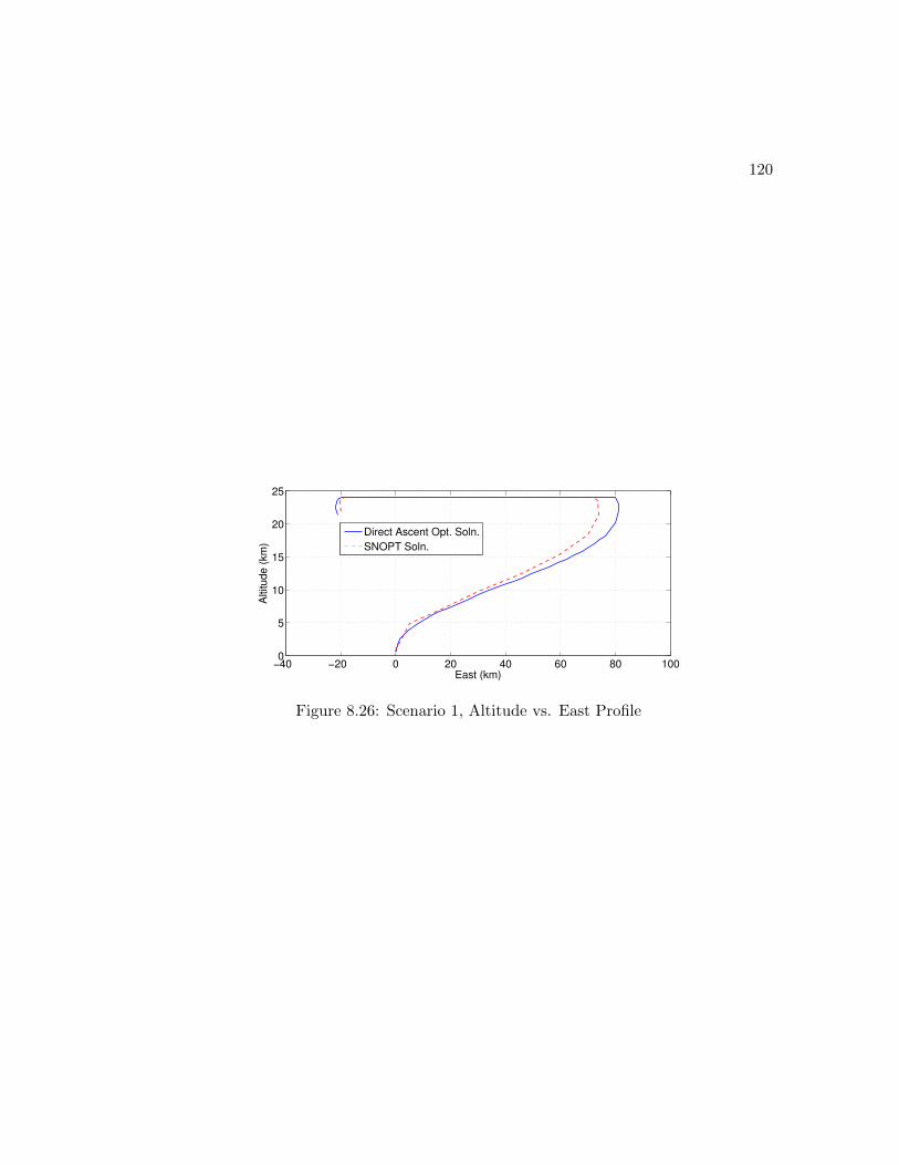
120
−40 −20 0 20 40 60 80 1000
5
10
15
20
25
East (km)
Altitude (
km
)
Direct Ascent Opt. Soln.
SNOPT Soln.
Figure 8.26: Scenario 1, Altitude vs. East Profile
Chapter 9
Conclusions
9.1 Summary
Stratospheric airships are an emerging class of autonomous, lighter-than-air vehicles.
With the capability to maintain a fixed geographic station at much lower altitudes than
satellites, these vehicles have the potential to perform a variety of long-term missions,
such as wireless telecommunications; remote sensing for weather monitoring and scien-
tific study; and imaging surveillance for traffic, border security, military operations and
search and rescue missions. The recognition of this potential is evident in the recent
widespread research and development of stratospheric airship platforms by academic,
military and industrial institutions around the world.
Because of their extremely large surface area to mass ratio, airship flight dynamics
are strongly influenced by the wind. A particular challenge for airship operation is
the planning of ascent trajectories, as the slow moving vehicle must traverse the high
speed winds of the jet stream. Due to the large changes in wind across altitude and
the susceptibility of airship motion to wind, the optimization of ascent trajectories is
important to ensure that the desired station is reached within acceptable performance
bounds of flight time, energy consumption, and lateral excursion.
121

122
The goal of this thesis was to perform a systematic study of optimal ascent trajectories
for stratospheric airships. A dynamic model of a generic airship configuration was
developed to facilitate trajectory analysis and design. The equations of motion were
derived for a point-mass model with aerodynamic lift and drag, buoyancy, thrust vector
control, added mass effects, and wind rate accelerations. The environment models were
developed, including polynomial fits for standard atmospheric density and a steady-state
horizontal wind model with altitude dependence. A model for solar power generation
was also developed, which describes the potential solar energy accumulation of solar
cells on a portion of the hull as a function of latitude, time of the day, day of the year,
and the airship orientation. Optimization problem formulations were then developed
for both minimum time and minimum energy ascent flights. Numerical solutions were
obtained through direct transcription and collocation of the original optimal control
problem. Here the dynamics of the system are discretized at a finite number of points,
so that the states and controls at each time become decision variables, and the dynamics
form equality constraints.
This model was used as the basis for developing different sets of optimal ascent
trajectories. Scenarios with fixed initial and final positions were considered and illustrate
the range of solutions between minimum-time and minimum-energy flights. We then
extended this formulation to study optimal trajectories over a range of initial conditions.
This provided crucial insights into the effect of wind gradients, and revealed a general
strategy for selecting the launch location.
Performance aspects of the optimal ascent trajectories were then analyzed. A solar
production model was developed that includes seasonal and diurnal effects, hull geome-
try effects, atmospheric losses, and the attitude of the vehicle. This was used in combi-
nation with various optimal ascent trajectories to compute net energy profiles resulting
from time-varying power production and consumption. It was found that some ascent
trajectories, while optimized with respect to the given wind profile, led to significant re-
ductions in power production due to the limited exposure of its top-mounted solar cells
123
to the sun. A sensitivity analysis was also performed, where trajectory optimizations
were re-computed across a range of drag coefficients and peak wind magnitudes. The
flight time and total energy of the flights were found to change by only a few percent,
and the optimal trajectories retained a consistent structure over all parameter values.
Finally, alternative methods were developed to more rapidly compute near-optimal as-
cent trajectories. This work was motivated by the need to quickly and reliably generate
achievable trajectory plans for onboard implementation. The structures and character-
istics of previously developed minimum-time and minimum-energy ascent trajectories
were studied, which led to the development of simplified trajectory models. These mod-
els essentially capture the general structure of the expected optimal ascent, enabling an
optimization over a small number of parameters to be performed quickly. Comparison of
these alternative solutions to the original SNOPT solutions show excellent agreement,
suggesting the alternate formulations are an effective means to develop near-optimal
solutions in an onboard setting.
9.2 Contributions
This work provides the first complete study of modeling, trajectory optimization and
proposed onboard guidance methods for stratospheric airships. In addition, it is among
the first works to develop a dynamic model with buoyancy, added mass and wind rate
terms, and to develop optimal trajectories for ascent. The key contributions are sum-
marized below.
• The development and characterization of optimal ascent trajectories for strato-
spheric airships for minimum-time and minimum-energy flights.
• Sensitivity analysis of optimal solutions with respect to variations in drag and
wind model characteristics.
• Modeling of solar irradiance exposure during ascent flights that account for time
124
of day, time of year, geographic latitude, altitude, and inertial orientation of the
airship.
• Modeling of predicted wind profiles that are suitable for use in trajectory planning.
• The development of an ascent guidance method that is amenable for onboard
implementation. This method enables computationally efficient re-planning of
the optimal trajectory subject to changes in the predicted wind profile.
Chapter 10
Recommendations for Future
Work
This thesis has established a foundational airship model and preliminary trajectory
optimization results that can be expanded in several different ways. Recommendations
for future work are summarized briefly below.
Analysis of the ascent trajectories found that ballast control uses about 10% of the
total energy for minimum-energy flights. However, this energy consumption was ne-
glected in the optimization. Adding a model of the power required for ballast control
to the numerical optimization would enable us to minimize the total energy. It could
also lead to different characteristics for minimum energy flights, as the power required
for ballast control varies with altitude and climb rate.
The scope of trajectory optimization has been limited to ascent flights. It would
be interesting to plan optimal descent flights using the same model. I suspect that
the structure of optimal solutions identified for ascent flights would also be present in
descent trajectories. For descent, however, additional altitude constraints would need
to be enforced so that the airship only descends to the ground once it is sufficiently
close to the landing site.
125

126
Long distance transfers between high-altitude stations is another interesting problem.
Developing trajectories for a long-distance transfer would require the wind model to ac-
count for variations in the wind profile over latitude, longitude and time. A particularly
interesting problem would be to utilize changes in the wind direction to cover large but
bounded geographic areas with minimal energy.
The ascent trajectories computed in this thesis have been based on a few different
representative wind profiles. The same planning methodologies can be applied with
wind profiles that are based on real-time winds aloft data provided by NOAA (National
Oceanic and Atmospheric Administration). This approach could be used with a set
of potential wind profiles to determine the best initial heading and approximate flight
duration. Alternatively, it would be interesting to develop a stochastic optimization
technique that guarantees certain performance metrics, such as flight time or energy,
remain within stated bounds subject to bounded changes in the assumed wind profile.
Finally, further work should be done to design and integrate a complete feedback
control policy that tracks the commanded angle of attack and heading throughout the
flight.
References
[1] G. A. Khoury and J. D. Gillett. Airship Technology. Cambridge Aerospace Series:
10, 1999.
[2] S. Lee and H. Bang. Three-Dimensional Ascent Trajectory Optimization for Strato-
spheric Airship Platforms in the Jet Stream. Journal of Guidance, Control, and
Dynamics, 30(5):1341–1352, 2007. doi: 10.0731-5090/07.
[3] D. K. Schmidt, J. Stevens, and J. Roney. Near-Space Station-Keeping Performance
of a Large High-Altitude Notional Airship. Journal of Aircraft, 44(2):611 – 615,
April 2007. doi: 10.0021-8669/07.
[4] D. K. Schmidt. Modeling and Near-Space Stationkeeping Control of a Large High-
Altitude Airship. Journal of Guidance, Control, and Dynamics, 30(2):540–547,
2007.
[5] A. Colozza. Initial Feasibility Assessment of a High Altitude Long Endurance
Airship. Technical Report NASA CR-2003-212724, NASA, Dec. 2003.
[6] T. C. Tozer and D. Grace. High Altitude Platforms for Wireless Communications.
Electronics and Communications Journal, 13(3):127–137, June 2001.
[7] C. Miller, J. Sullivan, and S. McDonald. High Altitude Airship Simulation Con-
trol and Low Altitude Flight Demonstration. In AIAA Infotech@Aerospace 2007
127
128
Conference and Exhibit, number AIAA 2007-2766, Rohnert Park, CA, May 2007.
AIAA Infotech@Aerospace.
[8] Th. Lutz and S. Wagner. Drag Reduction and Shape Optimization of Airship
Bodies. Journal of Aircraft, 35(3):345–351, 1997.
[9] S. Gomes and J. Ramos. Airship Dynamic Modeling for Autonomous Operation.
In IEEE International Conference on Robotics & Automation, Leuven, Belgium,
May 1998. IEEE.
[10] M. Battipede and P. Gil. Peculiar Performance of a New Lighter-Than-Air Platform
for Monitoring. In 3rd Unmanned Unlimited Technical Conference, Workshop &
Exhibit, number AIAA-6448, Chicago, IL, Sep 20-22 2004.
[11] S. Lee, H. Lee, D. Won, and H. Bang. Backstepping Approach of Trajectory
Tracking Control for the Mid-Altitude Unmanned Airship. In AIAA Guidance,
Navigation and Control Conference and Exhibit, number AIAA-2007-6319, Hilton
Head, SC, Aug. 2007.
[12] F. Repoulias and E. Papadopoulos. Dynamically feasible trajectory and open-loop
control design for unmanned airships. In Mediterranean Conference on Control &
Automation, pages 1–6, June 2007. doi: 10.1109/MED.2007.4433820.
[13] N. Rooz and E. Johnson. Design and Modelling of An Airship Station Holding
Controller for Low Cost Satellite Operations. In AIAA Guidance, Navigation, and
Control Conference and Exhibit, number AIAA-2005-6200, San Francisco, CA, Aug.
2005.
[14] J. Kim, J. Keller, and V. Kumar. Design and verification of controllers for air-
ships. In IEEE/RSJ International Conference on Intelligent Robots and Systems,
volume 1, pages 54–60, Oct. 2003. doi: 10.1109/IROS.2003.1250605.
129
[15] E. Hygounenc and P. Soueres. Automatic airship control involving backstepping
techniques. In IEEE International Conference on Systems, Man and Cybernetics,
Oct. 2002.
[16] Y. J. Zhao, W. L. Garrard, and J. B. Mueller. Benefits of Trajectory Optimization
in Airship Flights. In AIAA 3rd “Unmanned Unlimited” Technical Conference,
Workshop and Exhibit, pages 1–14, 2004.
[17] J. B. Mueller, Y. J. Zhao, and W. L. Garrard. Optimal Ascent Trajectories for
Stratsospheric Airships Using Wind Energy. Journal of Guidance, Control, and
Dynamics, 32(4):1232–1245, July–Aug 2009.
[18] A. Colozza. Airships for Planetary Exploration. Technical Report NASA/CR-2004-
213345, NASA, Nov 2004.
[19] Ely de Paiva Jose Azinheira, Alexandra Moutinho. Airship Hover Stabilization
Using a Backstepping Control Approach. Journal of Guidance, Control, and Dy-
namics, 29(4):903–914, 2006.
[20] E. de Paiva, F. Benjovengo, S. Bueno, J. Azinheira, and A. Moutinho. Nonlinear
Control Approaches for an Autonomous Unmanned Robotic Airship. In 7th AIAA
ATIO Conf, 2nd CEIAT Int’l Conf on Innov. and Integr. in Aero. Sciences,17th
LTA Systems Tech. Conf., Belfast, Northern Ireland, Sep. 2007.
[21] S. Sharma, E.A. Kulczycki, and A. Elfes. Trajectory generation and path planning
for autonomous aerobots. In Jet Propulsion Lab., California Inst. of Technology,
Pasadena, CA, 2007. NASA Jet Propulsion Laboratory.
[22] S. Hima and Y. Bestaoui. Motion generation on trim trajectories for an autonomous
underactuated airship. In 4th International Airship Convention and Exhibition ,
Cambridge England, July 2002.
130
[23] T. Kampke and A. Elfes. Optimal aerobot trajectory planning for wind-based
opportunistic flight control. In IEEE/RSJ International Conference on Intelligent
Robots and Systems, volume 1, pages 67–74, Oct. 2003.
[24] J. B. Mueller and Y. J. Zhao. Development of an Aerodynamic Model and Control
Law Design for a High-Altitude Airship. In AIAA 3rd “Unmanned Unlimited”
Technical Conference, Workshop and Exhibit, number AIAA-6479, Chicago, IL,
2004. AIAA.
[25] L. B. Tuckerman. Inertia factors of ellipsoids for use in airship design. NACA
Report No. 210, 1926.
[26] U.S. Standard Atmosphere, 1976. Technical Report (NOAA-S/T 76-15672): Supt.
of Docs., US Govt. Print. Off.(Stock No. 003-017-00323-0), National Oceanic and
Atmospheric Administration, Washington, DC, 1976.
[27] A. E. Hedin, E. L. Fleming, A. H. Manson, F. J. Schmidlin, S. K. Avery, R. R.
Clark, S. J. Franke, G. J. Fraser, T. Tsuda, F. Vial, and R. A. Vincent. Empirical
Wind Model for the Upper, Middle and Lower Atmosphere. Journal of Atmospheric
and Terrestrial PhysicsVolume, 58(13):1421–1447, Sep. 1996.
[28] Horizontal Wind Model, HWM-93. http://uap-www.nrl.navy.mil/uap/.
[29] H. Wang, B. Song, and L. Zuo. Effect of High-Altitude Airship’s Attitude on
Performance of its Energy System. Journal Of Aircraft, 44(6):2077–2079, 2007.
[30] J.T. Betts. Survey of numerical methods for trajectory optimization. Journal of
Guidance, Control, and Dynamics, 21(2):193–207, 1998.
[31] D. Hull. Conversion of Optimal Control Problems Into Parameter Optimization
Problems. Journal of Guidance, Control, and Dynamics, 20(1):57–60, 1997.
131
[32] A.L. Herman and B.A. Conway. Direct Optimization Using Collocation Based on
High-Order Gauss-Lobatto Quadrature Rules. Journal of Guidance, Control, and
Dynamics, 19:592–599, 1996.
[33] P. E. Gill, W. Murray, and M. A. Saunders. SNOPT: An SQP Algorithm for
Large-Scale Constrained Optimization. SIAM Journal of Optimization, 12:979–
1006, 2002.
[34] R. Walterscheid. High-Altitude Wind Prediction and Measurement Technology
Assessment. Technical Report ATR-2009(5427)-1, Aerospace Corporation, 2009.
[35] MM5 Community Model, May 2010. http://www.mmm.ucar.edu/mm5/.
[36] The Weather Research and Forecasting Model, May 2010. http://www.
wrf-model.org.

Appendix A
Glossary and Acronyms
This appendix defines various terms and acronyms that are used throughout the thesis.
A.1 Glossary
• Ascent Cone - A right circular cone with its vertex at the airship, representing
a geometric region that can only be accessed by varying the heading.
• Ballonet – An airbag contained within the exterior envelope of the airship. An
airship uses ballonets to regulate buoyancy. Ballast air is pumped into the ballonet
to increase vehicle weight, and it is pumped out to reduce the vehicle weight.
• Virtual Target (VT) – The coordinates of the target station for the airship
defined in a wind-relative frame. This is a predicted target after applying the
expected cumulative drift from the wind.
A.2 Acronyms
132
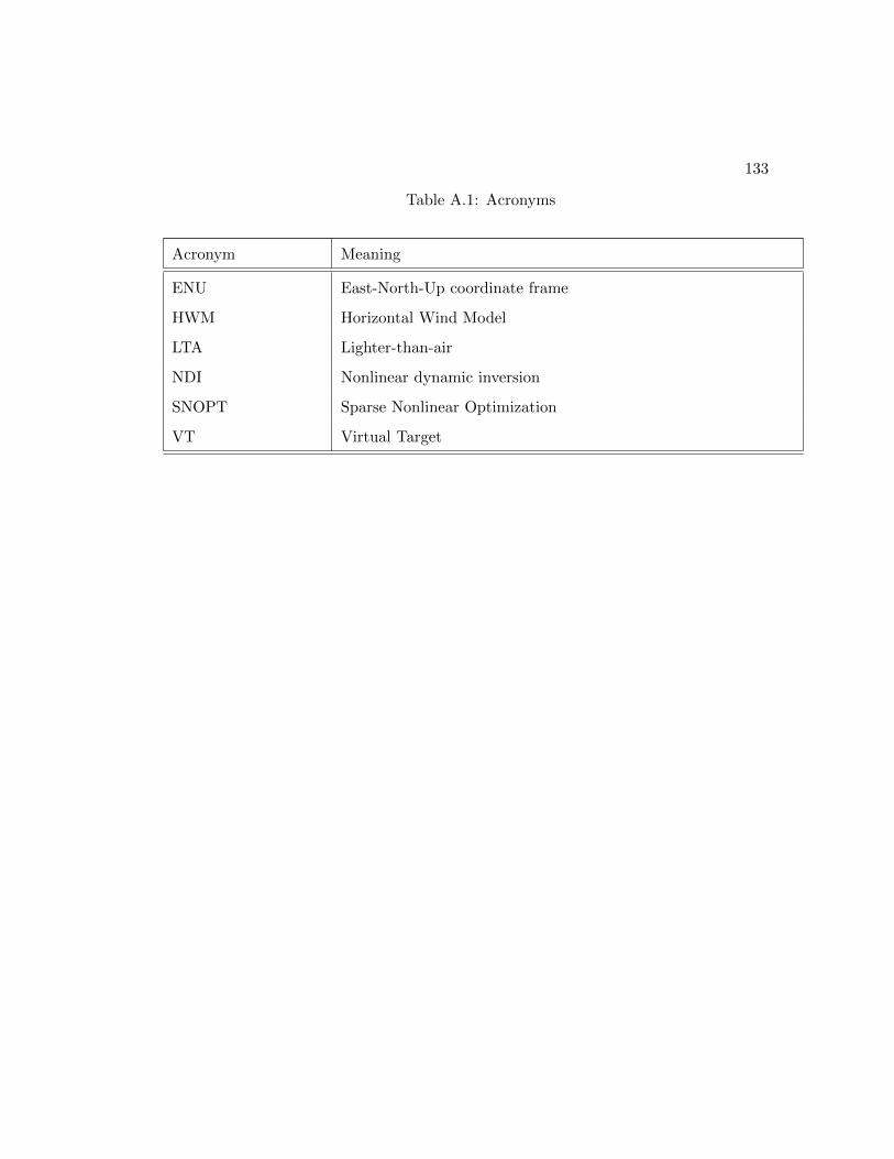
133
Table A.1: Acronyms
Acronym Meaning
ENU East-North-Up coordinate frame
HWM Horizontal Wind Model
LTA Lighter-than-air
NDI Nonlinear dynamic inversion
SNOPT Sparse Nonlinear Optimization
VT Virtual Target

Appendix B
Wind Prediction Model
This appendix summarizes the model used in this thesis for predicting wind profiles.
In order to plan the airship’s ascent trajectory, some prediction must be made of
the future winds to be encountered across different altitudes. The current wind profile
may be estimated using radar equipment or rapid ascent balloons [34]. However, these
methods may not be available, and even if they are, the winds may change from this
initial estimate by the time the airship reaches higher altitudes. In order to develop the
best possible prediction of winds aloft in real-time, existing wind modeling tools may
be used, such as the Mesoscale Model 5 [35] and the Weather and Research Forecast
(WRF) Model [36]. While these models have been found to provide a precision as good
as 5 m/s up to 20 km altitude [34], it is not known if they are suitable for a real-time,
onboard implementation.
Rather than focusing on a particular forecasting approach, the present objective is
to develop a representative model of a wind prediction method. From the perspective
of the guidance system, it is important that the wind prediction model has: 1) periodic
updates of the predicted wind profile during ascent, and 2) model mismatch between the
predicted and true wind profiles. In this section, we develop a relatively simple method
for computing and updating a predicted wind profile during ascent by incorporating
134
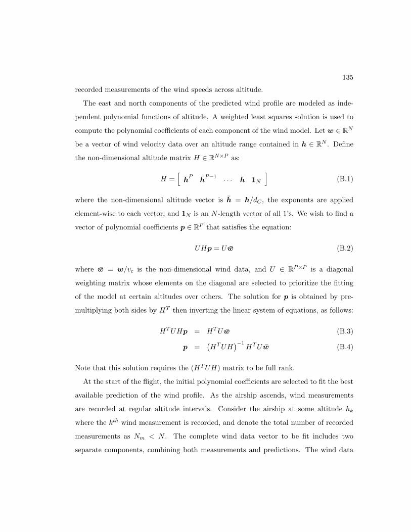
135
recorded measurements of the wind speeds across altitude.
The east and north components of the predicted wind profile are modeled as inde-
pendent polynomial functions of altitude. A weighted least squares solution is used to
compute the polynomial coefficients of each component of the wind model. Let w ∈ RN
be a vector of wind velocity data over an altitude range contained in h ∈ RN . Define
the non-dimensional altitude matrix H ∈ RN×P as:
H =[hP
hP−1 · · · h 1N
](B.1)
where the non-dimensional altitude vector is h = h/dC , the exponents are applied
element-wise to each vector, and 1N is an N -length vector of all 1’s. We wish to find a
vector of polynomial coefficients p ∈ RP that satisfies the equation:
UHp = Uw (B.2)
where w = w/vc is the non-dimensional wind data, and U ∈ RP×P is a diagonal
weighting matrix whose elements on the diagonal are selected to prioritize the fitting
of the model at certain altitudes over others. The solution for p is obtained by pre-
multiplying both sides by HT then inverting the linear system of equations, as follows:
HTUHp = HTUw (B.3)
p =(HTUH
)−1HTUw (B.4)
Note that this solution requires the (HTUH) matrix to be full rank.
At the start of the flight, the initial polynomial coefficients are selected to fit the best
available prediction of the wind profile. As the airship ascends, wind measurements
are recorded at regular altitude intervals. Consider the airship at some altitude hk
where the kth wind measurement is recorded, and denote the total number of recorded
measurements as Nm < N . The complete wind data vector to be fit includes two
separate components, combining both measurements and predictions. The wind data
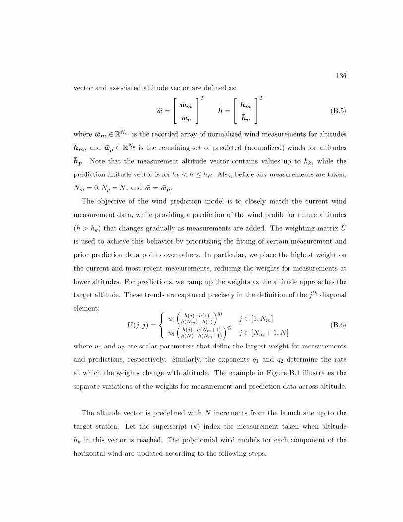
136
vector and associated altitude vector are defined as:
w =
wm
wp
T
h =
hm
hp
T
(B.5)
where wm ∈ RNm is the recorded array of normalized wind measurements for altitudes
hm, and wp ∈ RNp is the remaining set of predicted (normalized) winds for altitudes
hp. Note that the measurement altitude vector contains values up to hk, while the
prediction altitude vector is for hk < h ≤ hF . Also, before any measurements are taken,
Nm = 0, Np = N , and w = wp.
The objective of the wind prediction model is to closely match the current wind
measurement data, while providing a prediction of the wind profile for future altitudes
(h > hk) that changes gradually as measurements are added. The weighting matrix U
is used to achieve this behavior by prioritizing the fitting of certain measurement and
prior prediction data points over others. In particular, we place the highest weight on
the current and most recent measurements, reducing the weights for measurements at
lower altitudes. For predictions, we ramp up the weights as the altitude approaches the
target altitude. These trends are captured precisely in the definition of the jth diagonal
element:
U(j, j) =
u1
(h(j)−h(1)h(Nm)−h(1)
)q1j ∈ [1, Nm]
u2
(h(j)−h(Nm+1)h(N)−h(Nm+1)
)q2j ∈ [Nm + 1, N ]
(B.6)
where u1 and u2 are scalar parameters that define the largest weight for measurements
and predictions, respectively. Similarly, the exponents q1 and q2 determine the rate
at which the weights change with altitude. The example in Figure B.1 illustrates the
separate variations of the weights for measurement and prediction data across altitude.
The altitude vector is predefined with N increments from the launch site up to the
target station. Let the superscript (k) index the measurement taken when altitude
hk in this vector is reached. The polynomial wind models for each component of the
horizontal wind are updated according to the following steps.
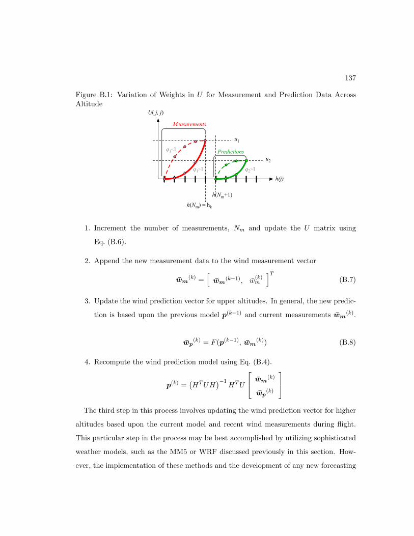
137
Figure B.1: Variation of Weights in U for Measurement and Prediction Data AcrossAltitude
q2>1q1>1
q1<1
h(Nm+1)
h(Nm) = hk
Predictions
Measurements
u1
h(j)
U( j, j)
u2
1. Increment the number of measurements, Nm and update the U matrix using
Eq. (B.6).
2. Append the new measurement data to the wind measurement vector
wm(k) =
[wm
(k−1), w(k)m
]T(B.7)
3. Update the wind prediction vector for upper altitudes. In general, the new predic-
tion is based upon the previous model p(k−1) and current measurements wm(k).
wp(k) = F (p(k−1), wm
(k)) (B.8)
4. Recompute the wind prediction model using Eq. (B.4).
p(k) =(HTUH
)−1HTU
wm
(k)
wp(k)
The third step in this process involves updating the wind prediction vector for higher
altitudes based upon the current model and recent wind measurements during flight.
This particular step in the process may be best accomplished by utilizing sophisticated
weather models, such as the MM5 or WRF discussed previously in this section. How-
ever, the implementation of these methods and the development of any new forecasting

138
methods is beyond the scope of this work. Because our present goal is to evaluate the
effect of wind model mismatch, we define the wind prediction vector as the true wind
plus some error. The following formulation is used:
wp(k) = (αk) wT + (1− αk) wp
(k−1) (B.9)
where wT is the true wind and 0 ≤ αk ≤ 1 is a weighting parameter that can be
varied across altitude. For the present analysis, we choose αk = k/N , which allows the
predicted wind speeds to steadily approach the true values as the airship ascends. At
the final altitude where a wind measurement is taken before reaching the station, we
have k = N , αN = 1 and wp(N) = wT .