Lecture # 12Lecture # 12

Cost CurvesCost Curves

Lecturer: Martin ParedesLecturer: Martin Paredes

2

1. Long Run Cost Functions Shifts Average and Marginal Cost Functions Economies of Scale Deadweight Loss

2. Long Run Cost Functions Relationship between Long Run and

Short Run Cost Functions

3

Definition: The long run total cost function relates the minimized total cost to output (Q) and the factor prices (w and r).

TC(Q,w,r) = wL*(Q,w,r) + r K*(Q,w,r)

where L* and K* are the long run input demand functions

4

Example: Long Run Total Cost Function Suppose Q = 50L0.5K0.5

We found:L*(Q,w,r) = Q . r 0.5 50 w

K*(Q,w,r) = Q . w 0.5 50 r

Then TC(Q,w,r) = wL*(Q,w,r) + rK*(Q,w,r)

= Q . (wr)0.5

25

( )( )

5

Definition: The long run total cost curve shows the minimized total cost as output (Q) varies, holding input prices (w and r) constant.

6

Example: Long Run Cost Curve Recall TC(Q,w,r) = Q . (wr)0.5

25 What if r = 100 and w = 25?

TC(Q,w,r) = Q . (25100)0.5

25= 2Q

7Q (units per year)

TC (€ per year)

TC(Q) = 2Q

Example: A Total Cost Curve

8Q (units per year)

TC (€ per year)

TC(Q) = 2Q

1 M.

€2M.

Example: A Total Cost Curve

9Q (units per year)

TC (€ per year)

TC(Q) = 2Q

1 M. 2 M.

€2M.

€4M.

Example: A Total Cost Curve

10

We will observe a movement along the long run cost curve when output (Q) varies.

We will observe a shift in the long run cost curve when any variable other than output (Q) varies.

11

L (labour services per year)

K

0

•L0

K0

Q0

TC = TC0

Example: Movement Along LRTC

12Q (units per year)

L (labour services per year)

K

TC (€/yr)

0

0

LR Total Cost Curve

Q0

TC0=wL0+rK0

•L0

K0

Q0

TC = TC0

Example: Movement Along LRTC

•

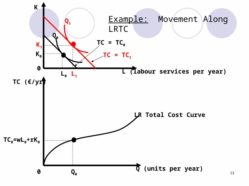
13Q (units per year)

L (labour services per year)

K

TC (€/yr)

0

0

LR Total Cost Curve

Q0

TC0=wL0+rK0

••

L0 L1

K0

K1

Q0

Q1

TC = TC1

TC = TC0

Example: Movement Along LRTC

•

14Q (units per year)

L (labour services per year)

K

TC (€/yr)

0

0

LR Total Cost Curve

Q0Q1

TC0=wL0+rK0

••

L0 L1

K0

K1

Q0

Q1

TC = TC1

TC = TC0

TC1=wL1+rK1

Example: Movement Along LRTC

••

15

Example: Shift of the long run cost curve

Suppose there is an increase in wages but the price of capital remains fixed.

16

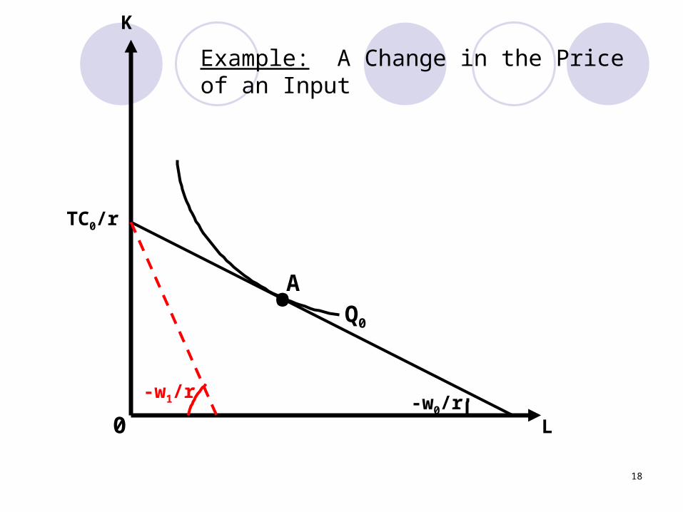
L

K

Q0

0

Example: A Change in the Price of an Input

17

L

K

Q0•

0

A

-w0/r

TC0/r

Example: A Change in the Price of an Input

18

L

K

Q0•

0

A

-w0/r

TC0/r

-w1/r

Example: A Change in the Price of an Input

19

L

K

Q0•

•

0

A

B

-w0/r

TC0/r

TC1/r

-w1/r

Example: A Change in the Price of an Input

TC1 > TC0

20

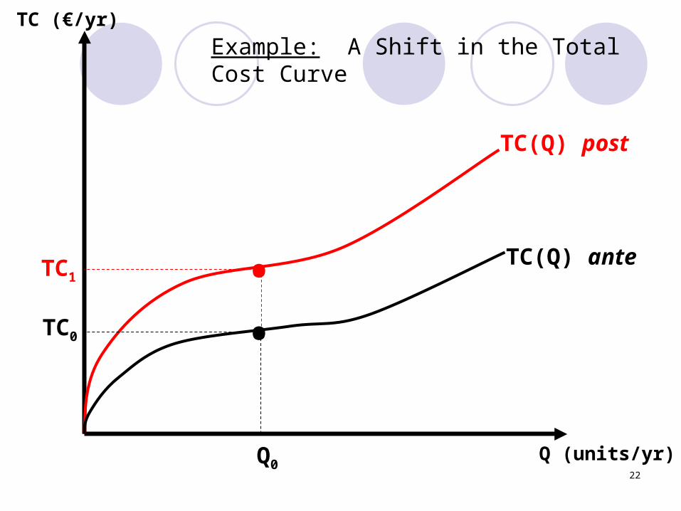
Q (units/yr)

TC (€/yr)

TC(Q) ante

Example: A Shift in the Total Cost Curve

21

Q (units/yr)

TC (€/yr)

TC(Q) ante

Q0

TC0

Example: A Shift in the Total Cost Curve

•

22

Q (units/yr)

TC (€/yr)

TC(Q) ante

TC(Q) post

Q0

TC1

TC0

Example: A Shift in the Total Cost Curve

••

23

Definition: The long run average cost curve indicates the firm’s cost per unit of output.

It is simply the long run total cost function divided by output.

AC(Q,w,r) = TC(Q,w,r)Q

24

Definition: The long run marginal cost curve measures the rate of change of total cost as output varies, holding all input prices constant.

MC(Q,w,r) = TC(Q,w,r) Q

25

Example: Average and Marginal Cost

Recall TC(Q,w,r) = Q . (wr)0.5

25

Then: AC(Q,w,r) = (wr)0.5

25MC(Q,w,r) = (wr)0.5

25

26

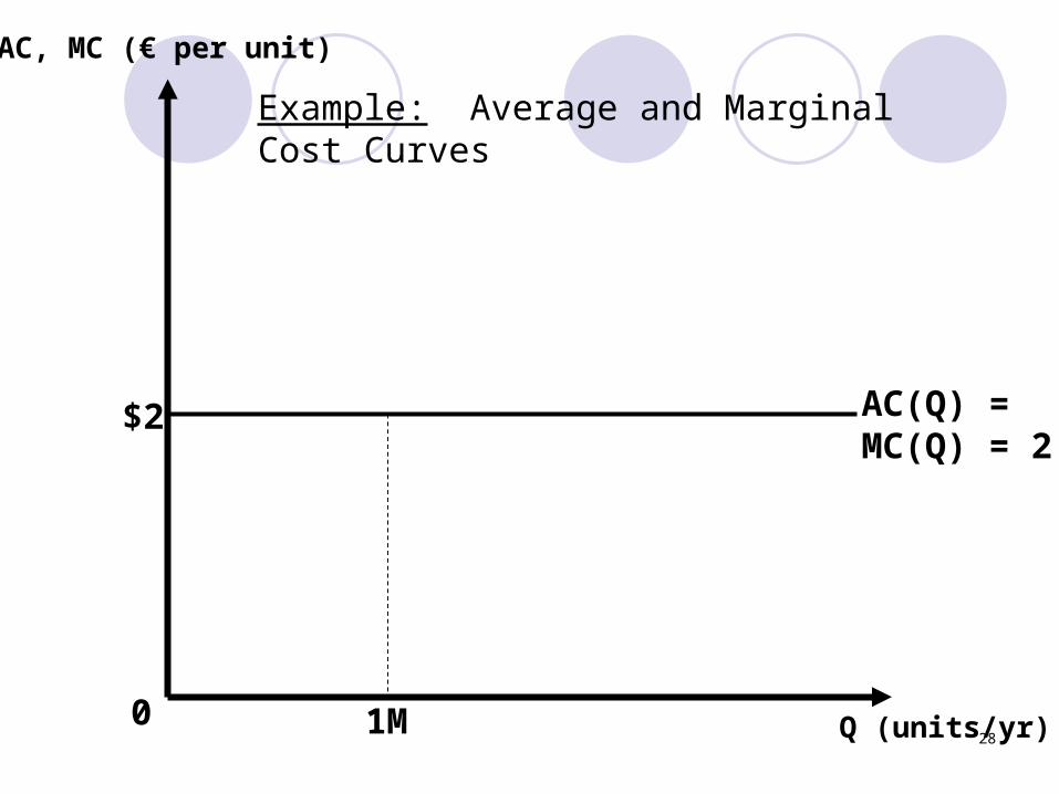
Example: Average and Marginal Cost

If r = 100 and w = 25, then TC(Q) = 2QAC(Q) = 2MC(Q) = 2

270

AC, MC (€ per unit)

Q (units/yr)

AC(Q) =MC(Q) = 2

$2

Example: Average and Marginal Cost Curves

280

AC, MC (€ per unit)

Q (units/yr)

AC(Q) =MC(Q) = 2

$2

Example: Average and Marginal Cost Curves

1M

290

AC, MC (€ per unit)

Q (units/yr)

AC(Q) =MC(Q) = 2

$2

Example: Average and Marginal Cost Curves

1M 2M

30

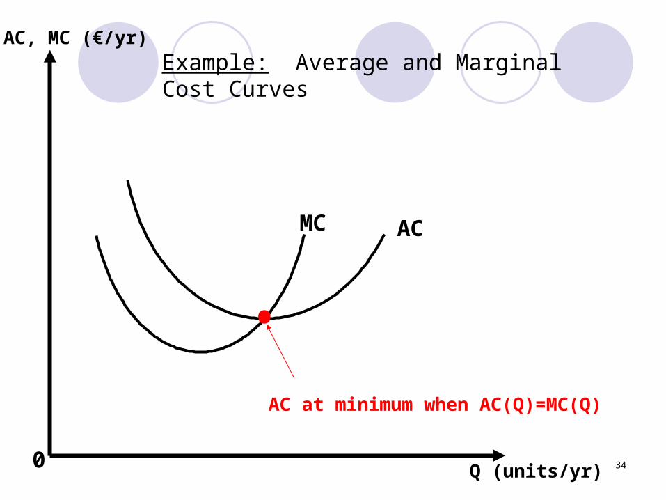
When marginal cost equals average cost, average cost does not change with output.

I.e., if MC(Q) = AC(Q), then AC(Q) is flat with respect to Q.

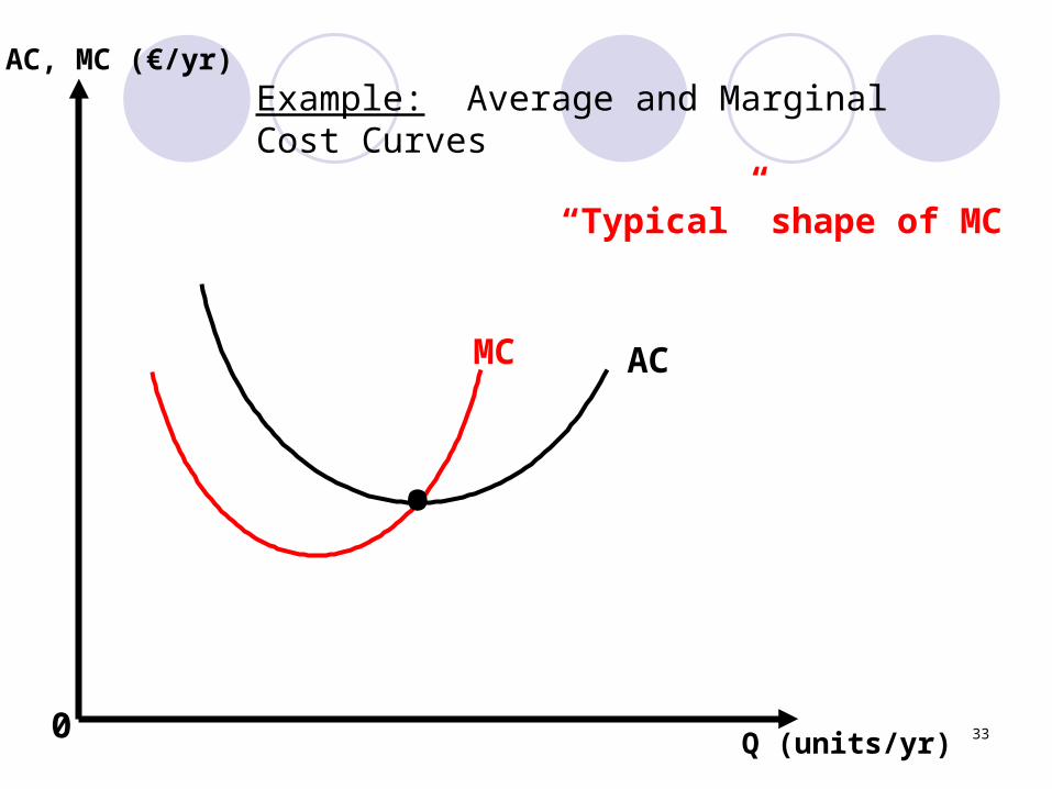
However, oftentimes AC(Q) and MC(Q) are not “flat” lines.

31

When marginal cost is less than average cost, average cost is decreasing in quantity.

I.e., if MC(Q) < AC(Q), AC(Q) decreases in Q.

When marginal cost is greater than average cost, average cost is increasing in quantity.

I.e., if MC(Q) > AC(Q), AC(Q) increases in Q.

We are implicitly assuming that all input prices remain constant.

32Q (units/yr)

AC, MC (€/yr)

0

AC

“Typical” shape of AC

Example: Average and Marginal Cost Curves

33Q (units/yr)

AC, MC (€/yr)

0

MC AC

“Typical” shape of MC

•

Example: Average and Marginal Cost Curves

34Q (units/yr)

AC, MC (€/yr)

0

MC AC

AC at minimum when AC(Q)=MC(Q)

•

Example: Average and Marginal Cost Curves

35

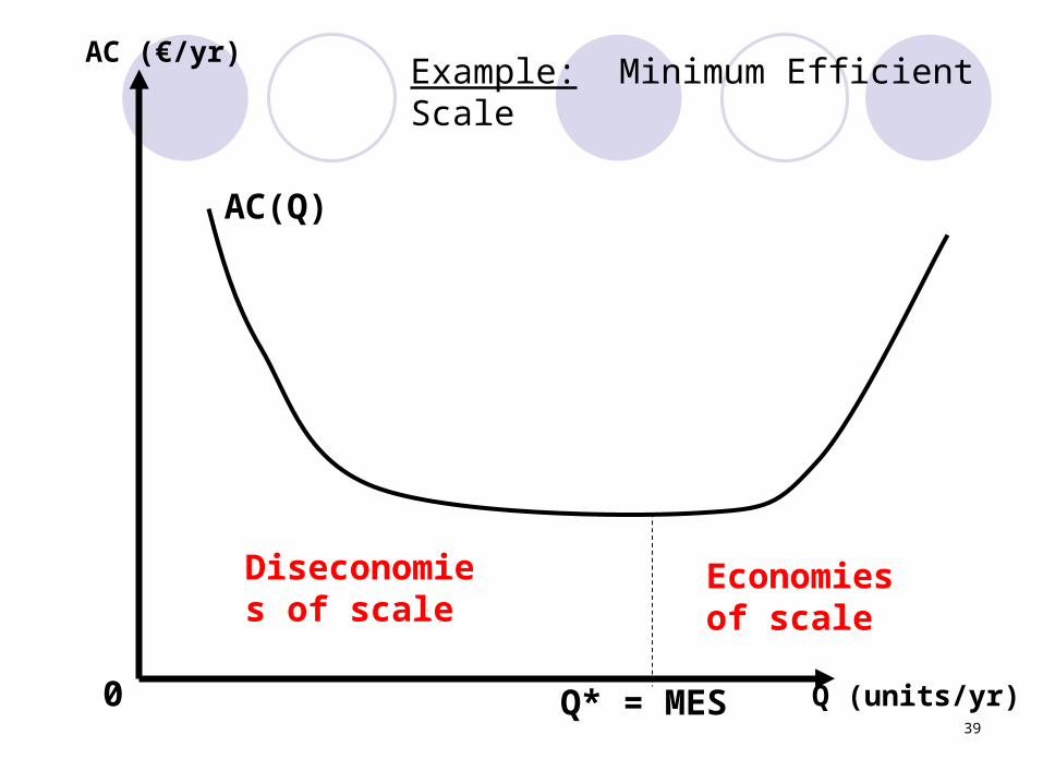
Definitions:1. If the average cost decreases as output

rises, all else equal, the cost function exhibits economies of scale.

2. If the average cost increases as output rises, all else equal, the cost function exhibits diseconomies of scale.

3. The smallest quantity at which the long run average cost curve attains its minimum point is called the minimum efficient scale.

36

0 Q (units/yr)

AC (€/yr)

AC(Q)

Example: Minimum Efficient Scale

37

0 Q (units/yr)

AC (€/yr)

Q* = MES

AC(Q)

Example: Minimum Efficient Scale

38

0 Q (units/yr)

AC (€/yr)

Q* = MES

AC(Q)

Example: Minimum Efficient Scale

Diseconomies of scale

39

0 Q (units/yr)

AC (€/yr)

Q* = MES

AC(Q)

Example: Minimum Efficient Scale

Diseconomies of scale

Economies of scale

40

Example: Minimum Efficient Scale for SelectedUS Food and Beverage Industries

Industry MES (% market output)

Beet Sugar (processed) 1.87Cane Sugar (processed) 12.01Flour 0.68Breakfast Cereal 9.47Baby food 2.59

Source: Sutton, John, Sunk Costs and Market Structure. MIT Press, Cambridge, MA, 1991.

41

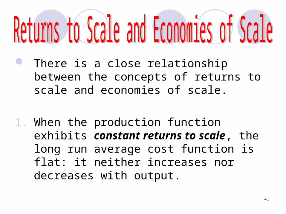
There is a close relationship between the concepts of returns to scale and economies of scale.

1. When the production function exhibits constant returns to scale, the long run average cost function is flat: it neither increases nor decreases with output.

42

2. When the production function exhibits increasing returns to scale, the long run average cost function exhibits economies of scale: AC(Q) increases with Q.

3. When . the production function exhibits decreasing returns to scale, the long run average cost function exhibits diseconomies of scale: AC(Q) decreases with Q.

43

Example: Returns to Scale and Economies of Scale

Returns to Scale DecreasingConstan

tIncreasing

Production Function Q = L0.5 Q = L Q = L2

Labour Demand L* = Q2 L* = Q L* = Q0.5

Total Cost Function TC = wQ2 TC = wQ

TC = wQ0.5

Average Cost Function

AC = wQ AC = wAC = wQ-

0.5

Economies of ScaleDiseconomi

esNone

Economies

44

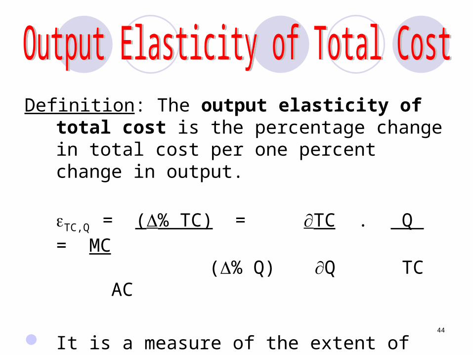
Definition: The output elasticity of total cost is the percentage change in total cost per one percent change in output.

TC,Q = (% TC) = TC . Q = MC (% Q) Q TC AC

It is a measure of the extent of economies of scale

45

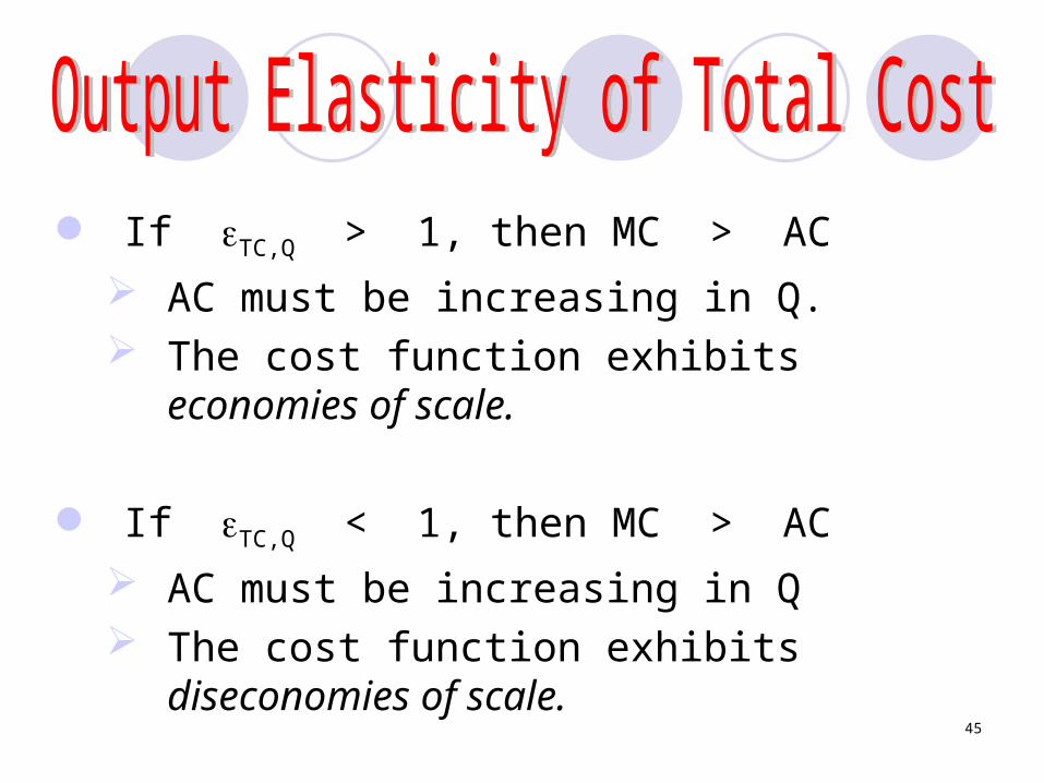
If TC,Q > 1, then MC > AC AC must be increasing in Q. The cost function exhibits economies of

scale.

If TC,Q < 1, then MC > AC AC must be increasing in Q The cost function exhibits diseconomies

of scale.

46

Example: Output Elasticities for Selected Manufacturing Industries in India

Industry TC,Q

Iron and Steel 0.553 Cotton Textiles 1.211Cement 1.162Electricity and Gas 0.3823

47

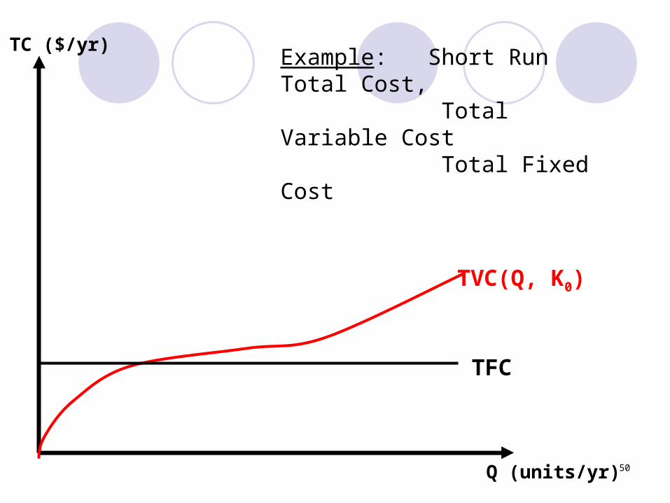
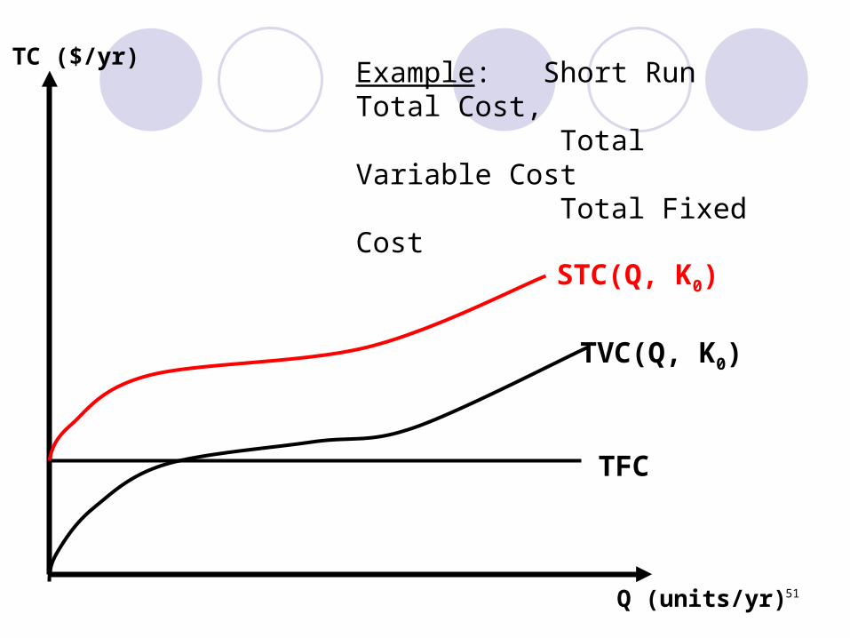
Definition: The short run total cost function tells us the minimized total cost of producing Q units of output, when (at least) one input is fixed at a particular level.

It has two components: variable costs and fixed costs:

STC(Q,K0) = TVC(Q,K0) + TFC(Q,K0)

(where K0 is the amount of the fixed input)

48

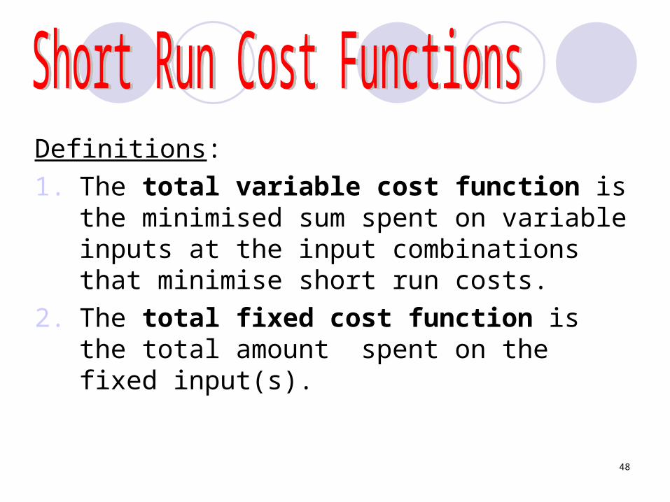
Definitions:1. The total variable cost function is the

minimised sum spent on variable inputs at the input combinations that minimise short run costs.

2. The total fixed cost function is the total amount spent on the fixed input(s).

49Q (units/yr)

TC ($/yr)

TFC

Example: Short Run Total Cost,

Total Variable Cost Total Fixed Cost

50Q (units/yr)

TC ($/yr)

TVC(Q, K0)

TFC

Example: Short Run Total Cost,

Total Variable Cost Total Fixed Cost

51Q (units/yr)

TC ($/yr)

TVC(Q, K0)

TFC

STC(Q, K0)

Example: Short Run Total Cost,

Total Variable Cost Total Fixed Cost

52Q (units/yr)

TC ($/yr)

TVC(Q, K0)

TFC

rK0

STC(Q, K0)

rK0

Example: Short Run Total Cost,

Total Variable Cost Total Fixed Cost

53

Example: Short Run Total Cost Suppose : Q = K0.5L0.25M0.25

w = €16m = €1r = €2

Recall the input demand functions:LS* (Q,K0) = Q2

4K0

MS*(Q,K0) = 4Q2

K0

54

Example (cont.): Short run total cost:

STC(Q,K0) = wLS* + mMS* + rK0

= 8Q2 + 2K0 K0

Total fixed cost:TFC(K0) = 2K0

Total variable cost:TVC(Q,K0) = 8Q2

K0

55

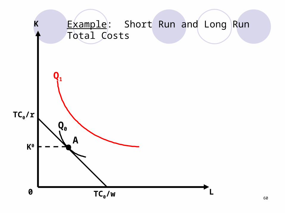
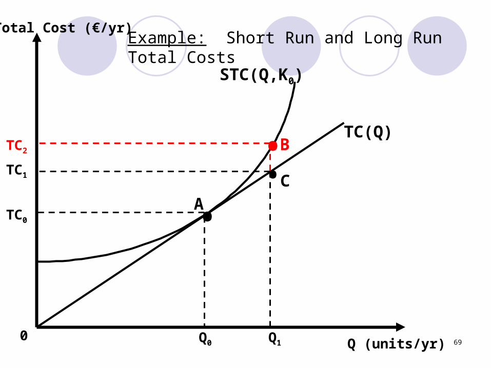
Compared to the short-run, in the long-run the firm is “less constrained”.

As a result, at any output level, long-run total costs should be less than or equal to short-run total costs:

TC(Q) STC(Q,K0)

56

In other words, any short run total cost curve should lie above the long run total cost curve.

The short run total cost curve and the long run total cost curve are equal only for some output Q*, where the amount of the fixed input is also the optimal amount of that input used in the long-run.

57L

K

0

Q0

Example: Short Run and Long Run Total Costs

58L

K

TC0/w

TC0/r

0

Q0

Example: Short Run and Long Run Total Costs

•A

59L

K

TC0/w

TC0/r

0

Q0

K0

Example: Short Run and Long Run Total Costs

•A

60L

K

TC0/w

TC0/r

0

Q1

Q0

K0

Example: Short Run and Long Run Total Costs

•A

61L

K

TC0/w

TC0/r

•

0

B

Q1

Q0

K0

Example: Short Run and Long Run Total Costs

•A

62L

K

TC0/w TC2/w

TC2/r

TC0/r

•

0

B

Q1

Q0

K0

Example: Short Run and Long Run Total Costs

•A

63L

K

TC0/w TC1/w TC2/w

TC2/r

TC1/r

TC0/r ••

0

C

B

Q1

Q0

K0

Example: Short Run and Long Run Total Costs

•A

64L

K

TC0/w TC1/w TC2/w

TC2/r

TC1/r

TC0/r •••

Expansion path

0

A

C

B

Q1

Q0

K0

Example: Short Run and Long Run Total Costs

65

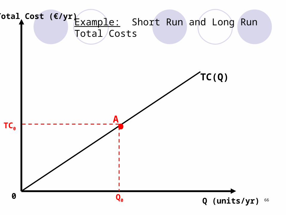
Example: Short Run and Long Run Total Costs

0Q (units/yr)

TC(Q)

Total Cost (€/yr)

66

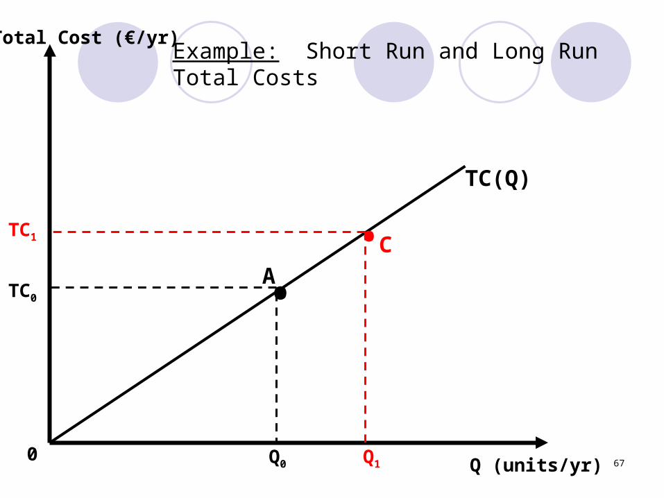
Example: Short Run and Long Run Total Costs

0Q (units/yr)

TC(Q)

•

Q0

ATC0

Total Cost (€/yr)

67

C

Example: Short Run and Long Run Total Costs

0Q (units/yr)

TC(Q)

•

Q0 Q1

•A

TC0

TC1

Total Cost (€/yr)

68

C

Example: Short Run and Long Run Total Costs

0Q (units/yr)

TC(Q)

STC(Q,K0)

•

Q0 Q1

•A

TC0

TC1

Total Cost (€/yr)

69

C

Example: Short Run and Long Run Total Costs

0Q (units/yr)

TC(Q)

STC(Q,K0)

•

Q0 Q1

••

A

B

TC0

TC1

TC2

Total Cost (€/yr)

70

C

Example: Short Run and Long Run Total Costs

0Q (units/yr)

TC(Q)

STC(Q,K0)

•

Q0

K0 is the LR cost-minimisingquantity of K for Q0

Q1

••

A

B

TC0

TC1

TC2

Total Cost (€/yr)

71

Definition: The short run average cost function indicates the short run firm’s cost per unit of output.

It is simply the short run total cost function divided by output, holding the input prices (w and r) constant.

SAC(Q,K0) = STC(Q,K0)Q

72

Definition: The short run marginal cost curve measures the rate of change of short run total cost as output varies, holding all input prices and fixed inputs constant.

SMC(Q,K0) = STC(Q,K0) Q

73

Notes: The short run average cost can be

decomposed into average variable cost and average fixed cost.

SAC = AVC + AFCwhere:

AVC = TVC/QAFC = TFC/Q

When STC = TC, then also SMC = MC

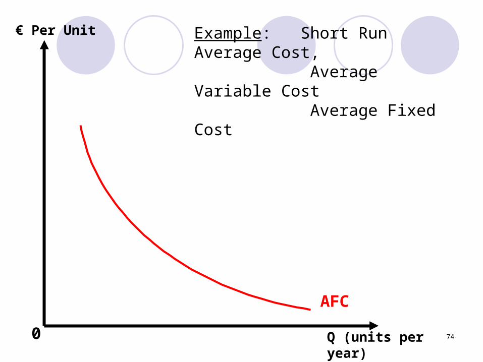
74Q (units per year)

€ Per Unit

0

AFC

Example: Short Run Average Cost,

Average Variable Cost Average Fixed Cost

75Q (units per year)

€ Per Unit

0

AVC

AFC

Example: Short Run Average Cost,

Average Variable Cost Average Fixed Cost

76Q (units per year)

€ Per Unit

0

SACAVC

AFC

Example: Short Run Average Cost,

Average Variable Cost Average Fixed Cost

77Q (units per year)

€ Per Unit

0

SMC SACAVC

AFC

Example: Short Run Average Cost,

Average Variable Cost Average Fixed Cost

78

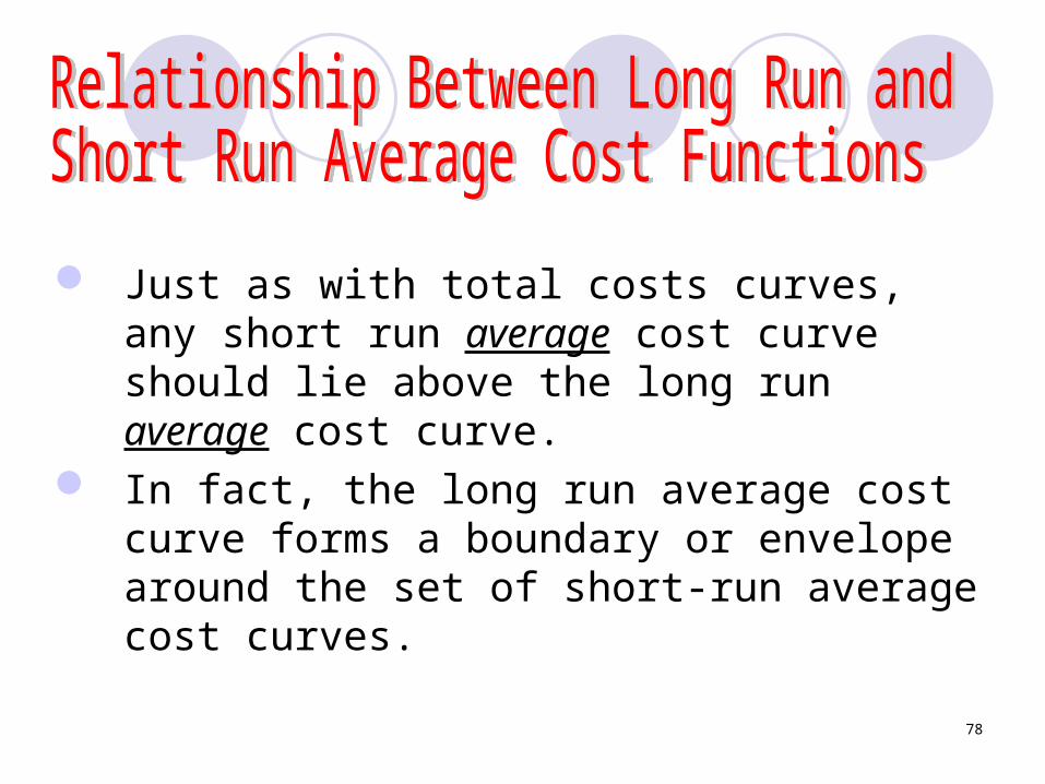
Just as with total costs curves, any short run average cost curve should lie above the long run average cost curve.

In fact, the long run average cost curve forms a boundary or envelope around the set of short-run average cost curves.

79

Q (units per year)

€ per unit

0

SAC(Q,K1)

The Long Run Average Cost Curve as an Envelope Curve

80

Q (units per year)

€ per unit

0

SAC(Q,K1)

SAC(Q,K2)

The Long Run Average Cost Curve as an Envelope Curve

81

Q (units per year)

€ per unit

0

SAC(Q,K1)

SAC(Q,K2)

The Long Run Average Cost Curve as an Envelope Curve

SAC(Q,K3)

82

Q (units per year)

€ per unit

0

SAC(Q,K1)

SAC(Q,K2)

The Long Run Average Cost Curve as an Envelope Curve

SAC(Q,K4)SAC(Q,K3)

83

Q (units per year)

€ per unit

0

• ••

SAC(Q,K1)

SAC(Q,K2)

Q1 Q2 Q3 Q4

The Long Run Average Cost Curve as an Envelope Curve

AC(Q)

SAC(Q,K4)

•

SAC(Q,K3)

84

1. Long run total cost curves plot the minimized total cost of the firm as output varies.

2. Movements along the long run total cost curve occur as output changes.

3. Shifts in the long run total cost curve occur as input prices change.

85

4. Average costs tell us the firm’s cost per unit of output.

5. Marginal costs tell us the rate of change in total cost as output varies.

6. Relatively high marginal costs pull up average costs, relatively low marginal costs pull average costs down.