lect 01© 2012 raymond p. jefferis iii1 satellite communications introduction general concepts...

Lect 01 © 2012 Raymond P. Jefferis III 1

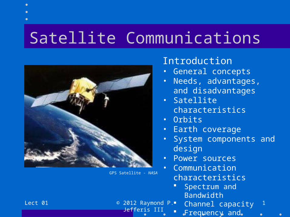
Satellite CommunicationsIntroduction • General concepts• Needs, advantages, and

disadvantages• Satellite characteristics• Orbits• Earth coverage• System components and design• Power sources• Communication characteristics

Spectrum and Bandwidth Channel capacity Frequency and Wavelength Path losses

Antennas and beam shaping

GPS Satellite - NASA


Text

• Text– Satellite Communications, Second Edition, T.

Pratt, C. Bostian, and J. Allnut, John Wilen & Sons, 2003.

Other Useful ReferencesIppolito, Louis J., Jr., Satellite Communications Systems Engineering, John Wiley,

2008.

Kraus, J. D., Electromagnetics, McGraw-Hill, 1953.

Kraus, J. D., and Marhefka, R. J., Antennas for All Applications, Third Edition, McGraw-Hill, 2002.

Morgan, W. L. , and Gordon, G. D., Communications Satellite Handbook, John Wiley & Sons, 1989.

Proakis, J. G., and Salehi, M., Communication Systems Engineering, Second Edition, Prentice-Hall, 2002.

Roddy, D, Satellite Communications, Fourth Edition, Mc Graw-Hill, 1989.

Stark, H., Tuteur, F. B., and Anderson, J. B., Modern Electrical Communications, Second Edition, Prentice-Hall, 1988.

Tomasi, W., Advanced Electronic Communications Systems, Fifth Edition, Prentice-Hall, 2001.



General Concepts of Satellites:

• They orbit around the earth– Have various orbital paths (to be discussed)

• They carry their own source of power

• They can communicate with:– Ground stations fixed on earth surface– Moving platforms (Non-orbital)– Other orbiting satellites


Needs, Advantages & Disadvantages

• Communications needs• Advantages of using satellites• Disadvantages of using satellites

Satellite Communications Needs

• Space vehicle to be used as communications platform(Earth-Space-Earth, Space-Earth, Space-Space)

• Space vehicle to be used as sensor platform with communications

• Ground station(s) (Tx/Rx)

• Ground receivers (Rx only)

•


List Advantages & Disadvantages


List these on the sheet supplied.

Five minutes allowed.

Advantages of Using Satellites

• High channel capacity (>100 Mb/s)

• Low error rates (Pe ~ 10-6)

• Stable cost environment (no long-distance cables or national boundaries)

• Wide area coverage (whole North America, for instance)

• Coverage can be shaped by antenna patterns


Disadvantages of Using Satellites

• Expensive to launch

• Expensive ground stations required

• Cannot be maintained

• Limited frequency spectrum

• Limited orbital space (geosynchronous)

• Constant ground monitoring required for positioning and operational control



Satellite Characteristics

• Orbiting platforms for data gathering and communications – position holding/tracking

• VHF, UHF, and microwave radiation used for communications with Ground Station(s)

• Signal path losses - power limitations• Systems difficult to repair and maintain• Sensitive political environment, with competing

interests and relatively limited preferred space

Mission Dependent Characteristics

• Orbital parameters– Height (velocity & period related to this)– Orientation (determined by application)– Location (especially for geostationary orbits)

• Power sources– Solar (principal), nuclear, chemical power– Stored gas/ion sources for position adjustment



Satellite Application Examples

• Telecommunications

• Military communications

• Navigation systems

• Remote sensing and surveillance

• Radio / Television Broadcasting

• Astronomical research

• Weather observation

Orbits

• Have particular advantages and disadvantages (See text Chapter 1)

• Are determined by satellite mission

• Keppler’s Laws of planetary motion describe certain orbital properties (Covered in Lecture 2)


Orbital Properties

• Altitude (radius to center of the earth)

• Inclination with respect to the earth axis

• Period of rotation about the earth

• Ground coverage by the satellite

• Communications path length(s)


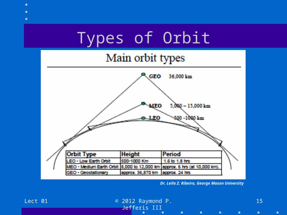
Types of Orbit


Dr. Leila Z. Ribeiro, George Mason University

Missions Associated with Orbit Types

• GEO– Primarily commercial communications

• MEO– Military and research uses

• LEO– Remote sensing– Global Positioning Systems

Lect 01 © 2012 Raymond P. Jefferis III Lect 01 - 16


LEO and MEO Features

• Earth coverage requires multiple passes

• Typical pass requires about 90 minutes

• Signal paths relatively short (lower losses)

• Small area, high resolution ground image

• Earth station tracking required• Multiple satellites for continuous coverage

(Decreases with increasing altitude - “Telstar”)


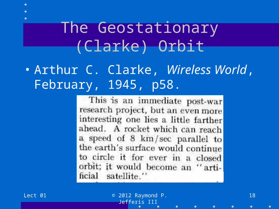
The Geostationary (Clarke) Orbit

• Arthur C. Clarke, Wireless World, February, 1945, p58.


Geo-Synchronous Satellite (GEO) Features

• Appears fixed over point on earth equator • Each satellite can cover 120 degrees latitude• Orbital Radius = 42,164.17 km• Earth Radius = 6,378.137 km (avg)• Period (Sidereal Day) = 23.9344696 hr

(86164.090530833 seconds)• Long signal path - large path losses


GEO Features (continued)

• Ground image area (instantaneous)

• Ground track coverage (multiple orbits)

• Stationarity (geostationary orbit)

• Space coverage (satellite-satellite)


Orbital Altitudes and Problems• Low Earth Orbit (LEO)

– 80 - 500 km altitude

– Atmospheric drag below 300 km

• Medium Earth Orbit (MEO)– 2000 - 35000 km altitude

– Van Allen radiation between 200 - 1000 km

• Geostationary Orbit (GEO)– 35,786 km altitude (42,164.57 km radius)

– Difficult orbital insertion and maintenance


Orbital Inclinations• Equatorial

– Prograde – inclined toward the east – Retrograde – inclined toward the west

• Inclined– Various inclination angles with respect to the

spin axis of the earth, including polar

• Geostationary (on equator; no inclination)

• Sun synchronous


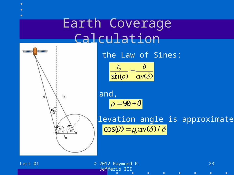
Earth Coverage Calculation

By the Law of Sines:

and,

rs

sin(ρ)=

dsin(δ )

ρ =90 +θ

The elevation angle is approximately,cos(θ) =rssin(δ ) / d

• The total coverage area on the surface of the earth, using the previously calculated value of δ) is given by the equation,

Earth Coverage Calculation (continued)


A =2πre2 (1−Cos[δ ])

Try the Calculation Yourself


Show Lect01S24calc.nb Mathematica®®program

Sample Calculation [Mathematica®]

re = 6378.137; (* km *)delta = 32.4171; (* degrees *)

area = 2 p re^2 (1 - Cos[delta Degree]);Print["Area = ", area, “[km^2]"]

Area = 3.98313*10^7 [km^2]


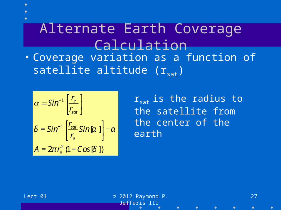
Alternate Earth Coverage Calculation

• Coverage variation as a function of satellite altitude (rsat)


α =Sin−1 re

rsat

⎡

⎣⎢

⎤

⎦⎥

δ = Sin−1 rsat

re

Sin[α ]⎡

⎣⎢

⎤

⎦⎥−α

A = 2π re2 (1− Cos[δ ])

rsat is the radius to the satellite from the center of the earth

Calculation: CoverageArea.nb

re = 6378.137; (* km *)rs = re + hs; alpha = ArcSin[re/rs]ad = alpha/Degreedelta = ArcSin[(rs/re)*Sin[alpha]] - alphadd = delta/DegreeA = 2 p re^2 (1.0 - Cos[delta])Plot[A, {hs, 1000, 2000}, AxesLabel -> "Coverage [km^2]", Frame -> True, FrameLabel -> {"Altitude [km]", "Coverage [km^2]"}]


Earth Coverage vs Satellite Altitude


Advanced Earth Coverage Calculations

In: Orbital Mechanics with MATLABhttp://www.cdeagle.com/html/ommatlab.html

Recommended download:Coverage Characteristics of Earth Satellites

http://www.cdeagle.com/ommatlab/coverage.pdf



“Satellite System” Components

• Satellite(s)

• Earth station(s)

• Computer systems

• Information network(Example: Internet)


Satellite System Design

Satellite network with earth stations.


Satellite Components• Receiver (receives on an uplink)

• Receiving antenna

• Signal processing (decode, security, encode, other)

• Transmitter (transmits on a downlink)

• Transmitting antenna (beam shaping)

• Power and environmental control systems

• Attitude control

• (De)multiplexing (used in rotating satellites)

• Position holding (mission dependent option)


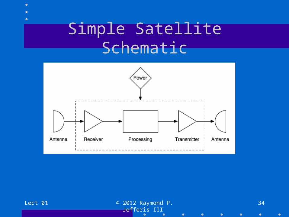
Simple Satellite Schematic


Satellite Power Sources

• Solar power panels (near-earth satellites)– Power degrades over time - relatively long

• Radioactive isotopes (deep space probes)– Lower power over very long life, rarely used.

• Fuel cells (space stations with resupply)– High power but need maintenance and chemical

resupply, rarely used.– Example: International Space Station


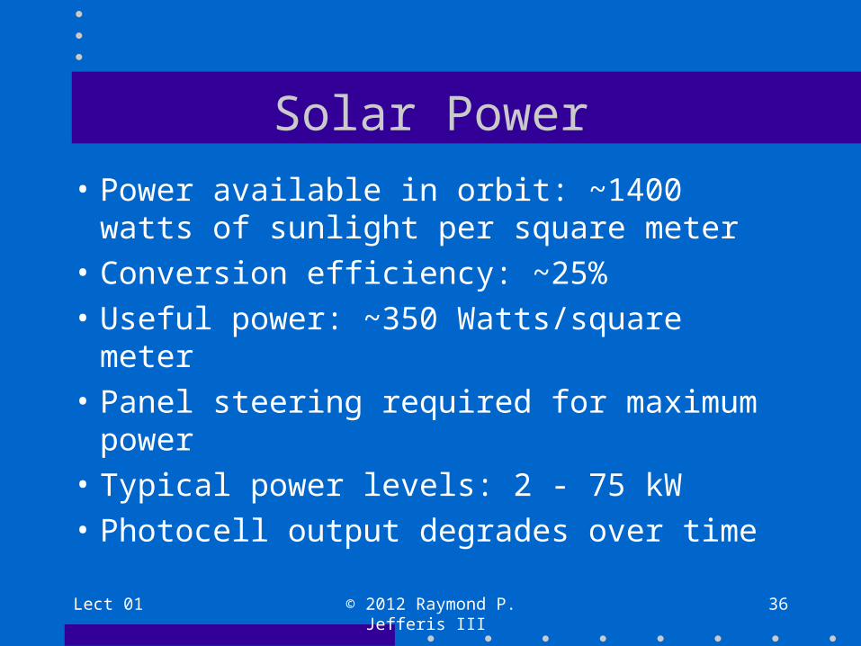
Solar Power

• Power available in orbit: ~1400 watts of sunlight per square meter

• Conversion efficiency: ~25%

• Useful power: ~350 Watts/square meter

• Panel steering required for maximum power

• Typical power levels: 2 - 75 kW

• Photocell output degrades over time


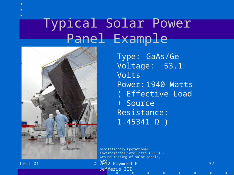
Typical Solar Power Panel Example

Geostationary Operational Environmental Satellites (GOES) - Ground testing of solar panels, NASA

Type: GaAs/GeVoltage: 53.1 VoltsPower: 1940 Watts( Effective Load + Source Resistance: 1.45341 Ω )

Satellite Communication Characteristics

• Via electromagnetic waves (“radio”)

• Typically at microwave frequencies

• High losses due to path length

• Many interference sources

• Attenuation due to atmosphere and weather

• High-gain antennas needed (“dish”) to make up for path loss and noise


Communication Characteristics (continued)

• Spectrum and Bandwidth

• Channel capacity

• Frequency and Wavelength

• Path losses


Spectrum and Bandwidth


• Electromagnetic spectrum allocations (“DC to light” – see next slide)

• Bandwidth: the size or “width” (in Hertz) of a spectrum frequency band

• Frequency band: a range of frequencies in the available spectrum.

• Channel capacity increases with the bandwidth (see Slide 42)

Electromagnetic Spectrum


Wikipedia

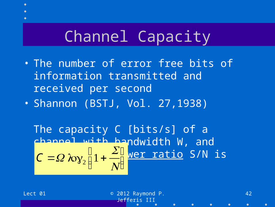
Channel Capacity

• The number of error free bits of information transmitted and received per second

• Shannon (BSTJ, Vol. 27,1938)

The capacity C [bits/s] of a channel with bandwidth W, and signal/noise power ratio S/N is


C =Wlog2 1+SN

⎛⎝⎜

⎞⎠⎟


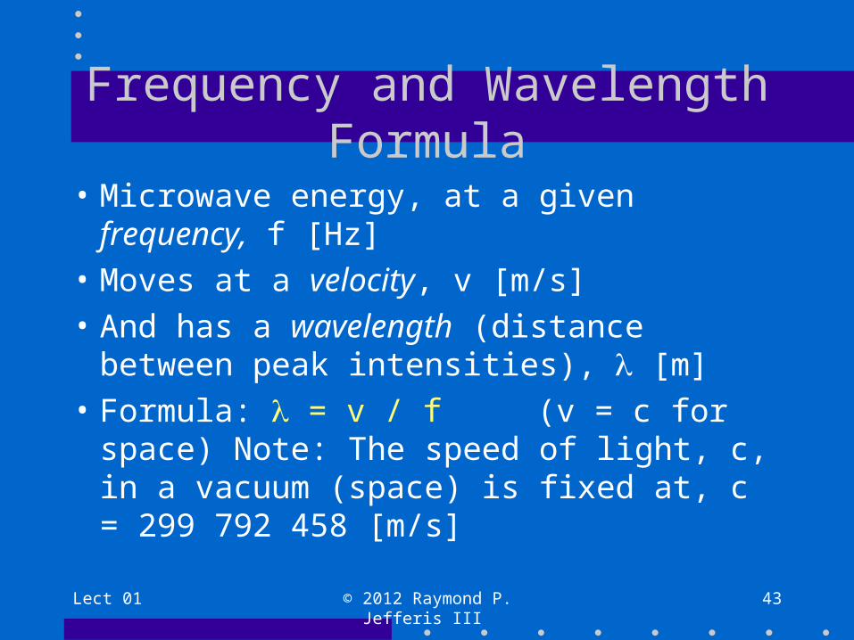
Frequency and Wavelength Formula

• Microwave energy, at a given frequency, f [Hz]

• Moves at a velocity, v [m/s]

• And has a wavelength (distance between peak intensities), λ [m]

• Formula: λ = v / f (v = c for space) Note: The speed of light, c, in a vacuum (space) is fixed at, c = 299 792 458 [m/s]

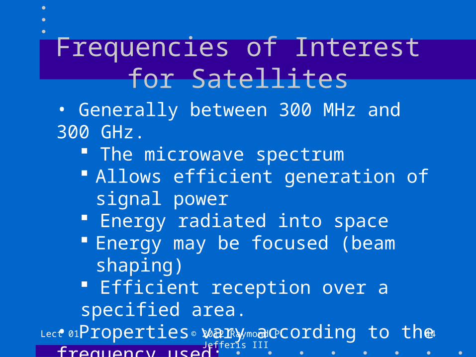
Frequencies of Interest for Satellites


• Generally between 300 MHz and 300 GHz. The microwave spectrum Allows efficient generation of signal power Energy radiated into space Energy may be focused (beam shaping) Efficient reception over a specified area.

• Properties vary according to the frequency used: Propagation effects (diffraction, noise, fading) Antenna Sizes

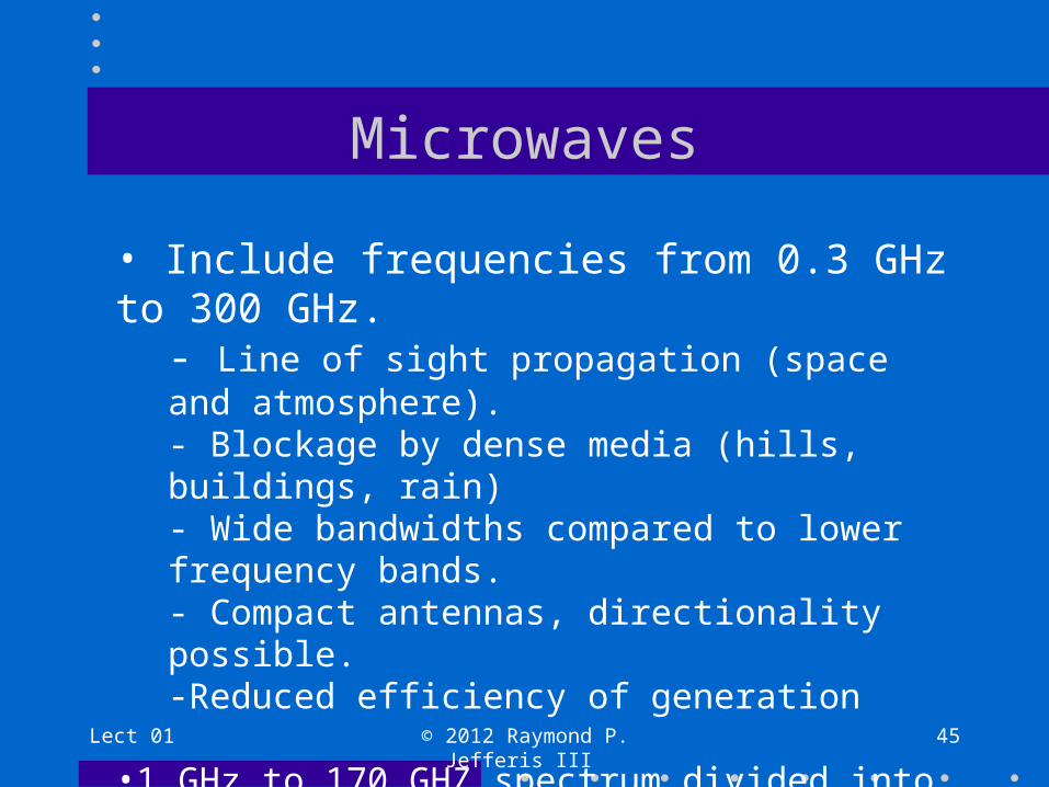
Microwaves


• Include frequencies from 0.3 GHz to 300 GHz. - Line of sight propagation (space and atmosphere).- Blockage by dense media (hills, buildings, rain)- Wide bandwidths compared to lower frequency bands.- Compact antennas, directionality possible.-Reduced efficiency of generation

•1 GHz to 170 GHZ spectrum divided into bands with letter designations (see next slide)

Designated Microwave Bands


Wikipedia

Standard designationsFor microwave bands

Common bands for satellite communication are the L, C and Ku bands.


Common Microwave Frequency Allocations

• L band 0.950 - 1.450 GHz Note: GPS at 1.57542 GHz

• C band 3.7 - 4.2 GHz (Downlink) 5.925 - 6.425 GHz (Uplink)

• Ku band 11.7 - 12.2 GHz (Downlink) 14 - 14.5 GHz (Uplink)


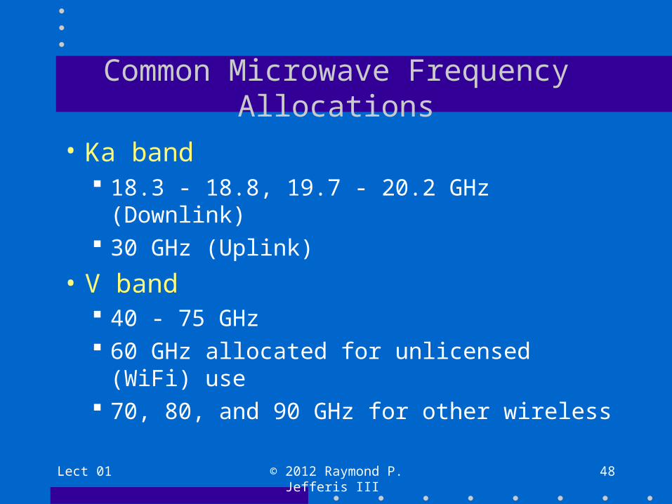
Common Microwave Frequency Allocations

• Ka band 18.3 - 18.8, 19.7 - 20.2 GHz (Downlink) 30 GHz (Uplink)

• V band 40 - 75 GHz 60 GHz allocated for unlicensed (WiFi) use 70, 80, and 90 GHz for other wireless

L-Band GPS Receiver



L-Band• Frequencies: 0.950 – 1.450 GHz (λ ~30cm)• Uses:

– Amateur radio communications

– GPS devices

• Features:– Patch antenna used for GPS receivers

– Low rain fade - Low atmospheric atten. (long paths)

– Low power

– Small receiver configurations


C-Band


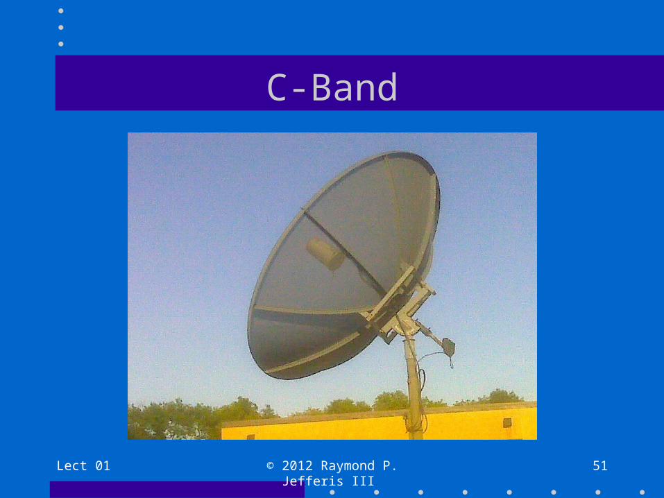
C-Band• Frequencies: 3.7 - 6.425 GHz (λ ~5cm)• Uses:

– TV reception (motels)

– IEEE-802.11 WiFi

– VSAT

• Features:– Large dish antenna needed (3m diameter)

– Low rain fade - Low atmospheric atten. (long paths)

– Low power - terrestrial microwave interferences


Ku-Band


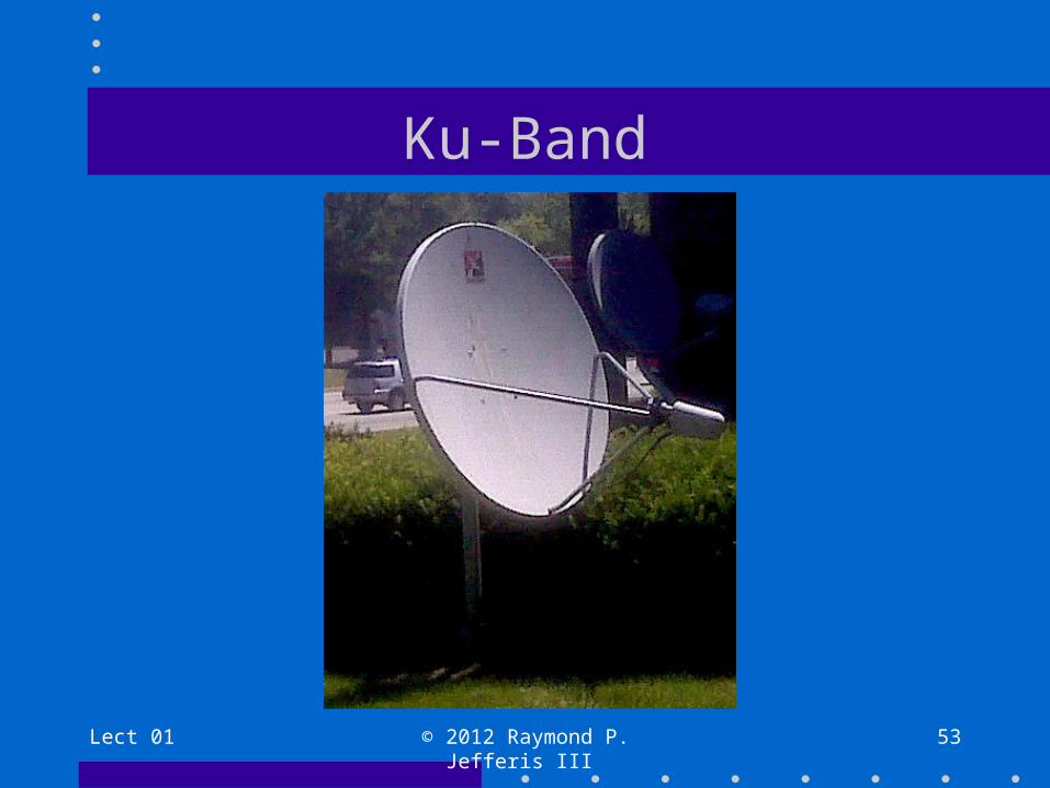
Ku-Band

• Frequencies: 12 - 18 GHz (λ ~ 2cm)• Uses:

– Remote TV broadcasting– Satellite communications– VSAT

• Features:– Rain, snow, ice (on dish) susceptibility– Small antenna size - high antenna gain– High power allowed


Ka-Band

• Frequencies: 18 - 40 GHz (λ~ 1cm)• Uses:

– High-resolution radar– Communications systems– Deep space communications

• Features:– Obstacles interfere (buildings, vegetation, etc.)– Atmospheric absorption


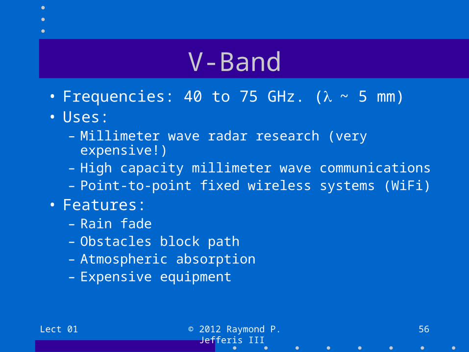
V-Band• Frequencies: 40 to 75 GHz. (λ~ 5 mm)• Uses:

– Millimeter wave radar research (very expensive!)– High capacity millimeter wave communications– Point-to-point fixed wireless systems (WiFi)

• Features:– Rain fade– Obstacles block path– Atmospheric absorption– Expensive equipment

Millimeter Waves

• Planck space exploration satellite– Planck is a flagship mission of the European Space Agency (Esa).

It was launched in May 2009 and moved to an observing position more than a million km from Earth on its "night side".It carries two instruments that observe the sky across nine frequency bands. The High Frequency Instrument (HFI) operates between 100 and 857 GHz (wavelengths of 3mm to 0.35mm), and the Low Frequency Instrument (LFI) operates between 30 and 70 GHz (wavelengths of 10mm to 4mm).

• Johnson noise problems addressed– Some of its detectors operate at minus 273.05C



Path Losses

• The loss of a radiated signal with distance• Losses increase with frequency• Satellites typically require long path lengths

( Path lengths can be over 42,000 km )

Causes of Path Loss

• Dispersion with distance• Atmospheric absorption (Calculated in

Lecture 11)• Rain, snow, ice, & cloud attenuation

(Calculated in Lecture 12)• Atmospheric noise effects resulting in

increased Bit Error Rate (BER) (Calculated in Lecture 6)



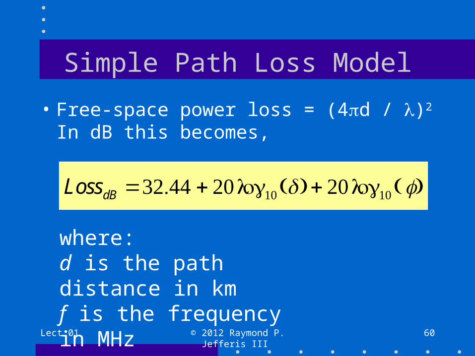
Simple Path Loss Model

• Free-space power loss = (4πd / λ)2

In dB this becomes,

LossdB =32.44 + 20 log10 (d) + 20 log10 ( f )

where:d is the path distance in kmf is the frequency in MHz


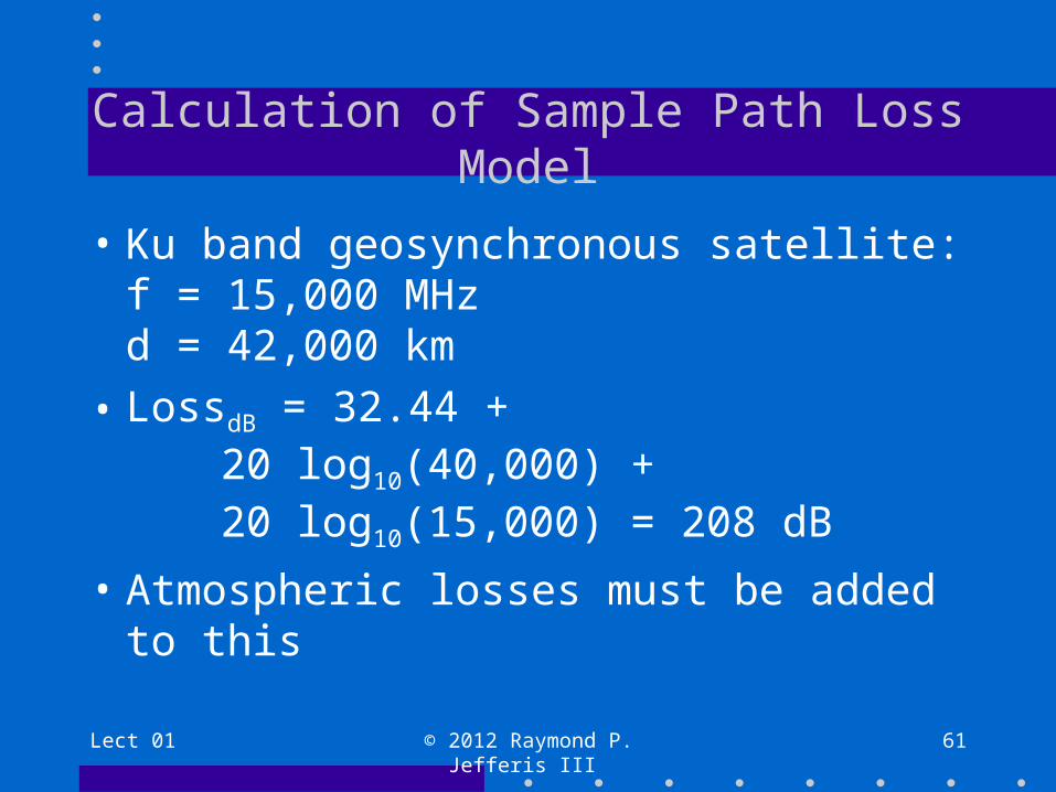
Calculation of Sample Path Loss Model

• Ku band geosynchronous satellite:f = 15,000 MHzd = 42,000 km

• LossdB = 32.44 + 20 log10(40,000) + 20 log10(15,000) = 208 dB

• Atmospheric losses must be added to this


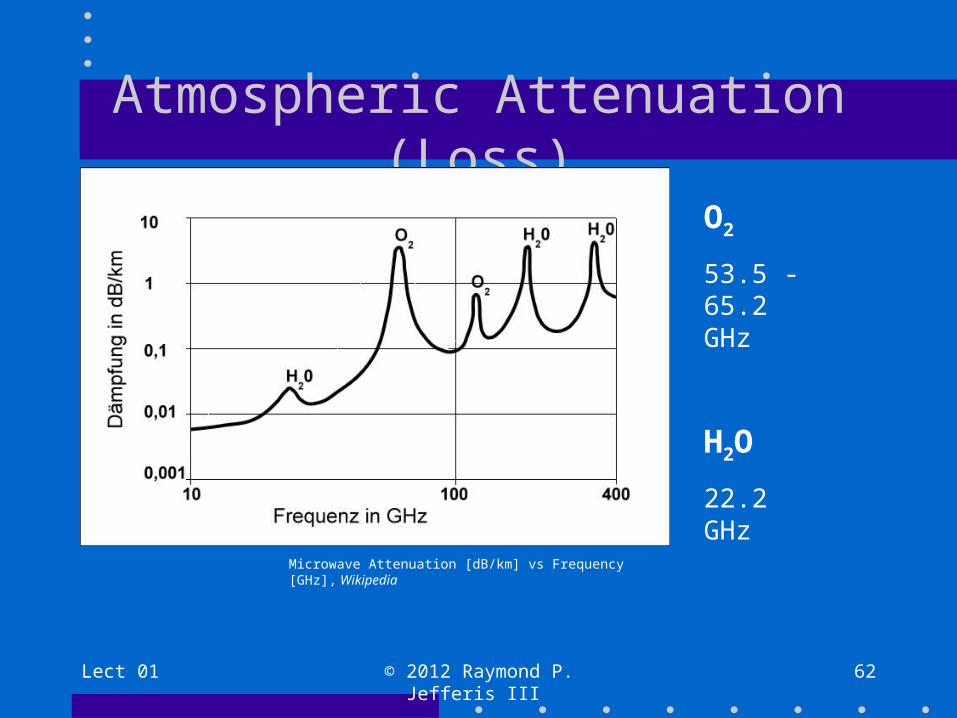
Atmospheric Attenuation (Loss)

Microwave Attenuation [dB/km] vs Frequency [GHz], Wikipedia

O2

53.5 - 65.2 GHz

H2O

22.2 GHz


H2O vs Dry Air Absorption (Loss)

Remedies for Path Loss

• High gain antennas• High transmitter power• Low-noise receivers• Tracking of steered antennas• Modulation techniques• Error correcting codes• Frequency selection• Beam shaping to focus energy



Constraints Limiting Path Loss Remedies

• Maximal antenna sizes push satellite radio wavelengths below 2m.

• Requirements for antenna gain, due to communication path losses, reduce the practical wavelengths to below 20cm. (Diameter, d, of many wavelengths, λ)

• Dish-Antenna Power Gain = η(πd/λ2

(where η is antenna efficiency)


Antenna Gain Calculation

• Ku-Band antenna Diameter 80 cm (d/λ = 40), η = 0.6

(about 40 wavelengths at 15GHz) Power Gain = 0.6*(3.14*40)2 = 15775

GdB = 10 log10[Power Gain ] = 40 dB

Note: Losses and sidelobe effects can reduce this gain to 60% or less of its possible value.


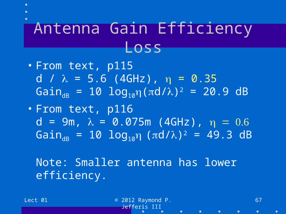
Antenna Gain Efficiency Loss

• From text, p115d / λ = 5.6 (4GHz), η = 0.35GaindB = 10 log10η(πd/λ)2 = 20.9 dB

• From text, p116d = 9m, λ= 0.075m (4GHz), η0GaindB = 10 log10η (πd/λ)2 = 49.3 dB

Note: Smaller antenna has lower efficiency.

Beam Shaping through Antenna Design

• Antenna radiation patterns (the beam) can be shaped to redistribute the radiated energy, by antenna design

• Shaping radiation patterns can increase signal strength in selected areas– Allows for more signal energy where higher

noise levels are expected– Allows energy to be conserved for areas of low

noise or low economic concern



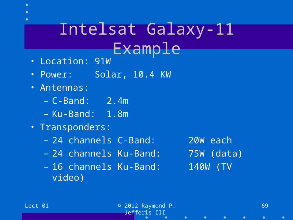
Intelsat Galaxy-11 Example• Location: 91W

• Power: Solar, 10.4 KW

• Antennas:

– C-Band: 2.4m

– Ku-Band: 1.8m

• Transponders:

– 24 channels C-Band: 20W each

– 24 channels Ku-Band: 75W (data)

– 16 channels Ku-Band: 140W (TV video)


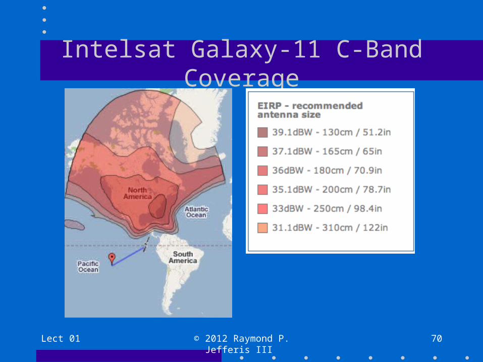
Intelsat Galaxy-11 C-Band Coverage


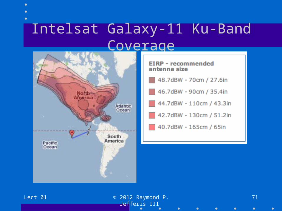
Intelsat Galaxy-11 Ku-Band Coverage


Conclusions

• Design constraints limit the power avaiable to satellite communications equipment

• Path losses limit communication capacity

• High gain antennas can overcome some limitations

• Antenna patterns can be shaped to favor desired locations on the earth

Questions?


Reminders

• Check access to a math package (Mathematica® or MATLAB®)

• Do homework


End


lect 01© 2012 raymond p. jefferis iii1 satellite communications introduction general concepts...

Documents