lateral torsional buckling of wood beams - … torsional buckling of wood beams by qiuwu xiao thesis...
TRANSCRIPT

Lateral Torsional Buckling of Wood Beams
by
Qiuwu Xiao
Thesis submitted to the
Faculty of Graduate and Postdoctoral Studies
in partial fulfillment of the requirements for the degree of
Master of Applied Science
in Civil Engineering
Under the auspices of the Ottawa-Carleton Institute for Civil Engineering
Departments of Civil Engineering
University of Ottawa
April 2014
© Qiuwu Xiao, Ottawa, Canada, 2014

i
Abstract
Structural wood design standards recognize lateral torsional buckling as an important failure
mode, which tends to govern the capacity of long span laterally unsupported beams. A survey
of the literature indicates that only a few experimental programs have been conducted on the
lateral torsional buckling of wooden beams. Within this context, the present study reports an
experimental and computational study on the elastic lateral torsional buckling resistance of
wooden beams.
The experimental program consists of conducting material tests to determine the longitudinal
modulus of elasticity and rigidity modulus followed by a series of 18 full-scale tests. The
buckling loads and mode shapes are documented. The numerical component of the study
captures the orthotropic constitutive properties of wood and involves a sensitivity analysis on
various orthotropic material constants, models for simulating the full-scale tests conducted, a
comparison with experimental results, and a parametric study to expand the experimental
database.
Based on the comparison between the experimental program, classical solution and FEA
models, it can be concluded that the classical solution is able to predict the critical moment of
wood beams. By performing the parametric analysis using the FEA models, it was observed
that loads applied on the top and bottom face of a beam decrease and increase its critical
moment, respectively. The critical moment is not greatly influenced by moving the supports
from mid-span to the bottom of the end cross-section.

ii
Acknowledgement
Special thanks go to my supervisors, Drs. Ghasan Doudak and Magdi Mohareb. Without their
great support, time, patience and advice, I would never have been able to complete this project.
I would also like to thank my fellow graduate students, Mr. Daniel Lacroix and Ms.
Ghazanfarah Hafeez for the guidance and help, especially in conducting the experimental work.
Also, thank you to Mr. Kevin Rocchi, Mr. Kenny Kwan. Mr. Christian Viau and Mr.
Mohammadmehdi Ebadi for their support.
My deepest thanks go to my parents for financial and moral supports, and for always
encouraging and believing in me to accomplish my academic goals.
iii
Table of Contents
Abstract ....................................................................................................................................... i
Acknowledgement ..................................................................................................................... ii
Table of Contents ..................................................................................................................... iii
List of Tables ............................................................................................................................. ix
List of Figures ........................................................................................................................... xi
Chapter 1-Introduction ............................................................................................................... 1
1.1. General ..................................................................................................................... 1
1.1.1. Wood Material Properties .................................................................................... 1
1.1.2 The Classical Solution Lateral Torsional Buckling Failure ............................. 5
1.1.3 Effective Length Approach .............................................................................. 9
1.1.4 Equivalent Moment Factor Approach ............................................................ 10
1.2. Research Objective ................................................................................................ 11
1.3. Research Methodology .......................................................................................... 12
1.4. Structure of The Thesis .......................................................................................... 12
1.5. Notation for Chapter 1 ........................................................................................... 13
1.6. References ............................................................................................................. 15
CHAPTER 2-Literature Review .............................................................................................. 16
2.1 Design Methods for Lateral Torsional Buckling of Beams ................................... 16
2.1.1 Development of Classical LTB Solution ........................................................ 16
2.2.2 The Development of Equivalent Moment Factor ........................................... 17
2.2.3 Development of Effective Length Approach on Timber Beams .................... 19
2.2.4 Effect of The Location of Load ...................................................................... 20
2.2.5. Continuous Rectangular Beams in Lateral Torsional Buckling ..................... 22

iv
2.2.6. Lateral Torsional Buckling for Cantilever of Rectangular Section ................ 23
2.2 Lateral Torsional Buckling Tests Related to Wood Members ............................... 24
2.2.1 Hooley and Madsen (1964) ............................................................................ 24
2.2.2 Hindman et al. (2005a) ................................................................................... 24
2.2.3 Hindman et al. (2005b)................................................................................... 25
2.2.4 Burow et al. (2006)......................................................................................... 25
2.2.5 Suryoatmono and Tjondro (2008) .................................................................. 25
2.2.6 Hindman (2008) ............................................................................................. 26
2.2.7 Bamberg (2009) .............................................................................................. 26
2.3 Notation for Chapter 2 ........................................................................................... 26
2.4 References ............................................................................................................. 27
Chapter 3-Sensitivity Analysis ................................................................................................. 30
3.1 General ................................................................................................................... 30
3.2 Model Description ................................................................................................. 31
3.2.1 Introduction .................................................................................................... 31
3.2.2 The Element Type and Mesh of Model .......................................................... 32
3.2.3 Eigenvalue Analysis ....................................................................................... 33
3.2.4 Mechanical Material Properties ..................................................................... 33
3.2.5 Boundary Conditions...................................................................................... 34
3.2.6 Constraints Related to The Longitudinal Degrees of Freedom ...................... 35
3.2.7 Load Application ............................................................................................ 37
3.3 Comparison with Classical LTB Solution ............................................................. 38
3.4 Sensitivity Analysis ............................................................................................... 40

v
3.5 Notation for Chapter 3 ........................................................................................... 43
3.6 References ............................................................................................................. 44
Chapter 4-Experimental Program ............................................................................................ 45
4.1 Introduction ........................................................................................................... 45
4.2 Torsional Test to Determine The Shear Modulus .................................................. 47
4.2.1 Torsion Test Set-up ......................................................................................... 47
4.2.2 Determining The Angle of Twist .................................................................... 51
4.3 Bending Test Set-up ............................................................................................... 52
4.4 Full-scale Lateral Torsional Buckling Test Set-up ................................................ 54
4.4.1 Boundary Conditions...................................................................................... 55
4.4.2 Load Application Mechanism ........................................................................ 56
4.4.3 Instrumentation............................................................................................... 57
4.5 Notation for Chapter 4 ........................................................................................... 61
4.6 References ............................................................................................................. 61
Chapter 5-Experimental Results .............................................................................................. 62
5.1 General ................................................................................................................... 62
5.2 Torsional Test Results ............................................................................................ 62
5.2.1 Calculation Method ........................................................................................ 62
5.2.2 Torsional Test to Failure ................................................................................. 62
5.2.3 Shear Modulus for Glulam Beams ................................................................. 64
5.2.4 Shear Modulus for Lumber ............................................................................ 66
5.3 Bending Test Results ............................................................................................. 70
5.3.1 Determining the Modulus of Elasticity of Glulam Beams about The Weak Axis
........................................................................................................................ 70

vi
5.3.2 Determining the Modulus of Elasticity of Lumber Joists about the Weak Axis
........................................................................................................................ 72
5.4 Results from the Full-scale Lateral Torsional Buckling Tests ............................... 76
5.5 Deformation and Typical Failure Modes ............................................................... 79
5.5.1 Deformed Shape ............................................................................................. 79
5.5.2 Typical Failure Modes .................................................................................... 82
5.6 Notation for Chapter 5 ........................................................................................... 84
5.7 References ............................................................................................................. 85
Chapter 6-Comparison Between FEA Model and Experimental Results ................................ 86
6.1 Model Description ................................................................................................. 86
6.1.1 Introduction .................................................................................................... 86
6.1.2 Mesh Details ................................................................................................... 86
6.1.3 Mechanical Properties of Material ................................................................. 88
6.1.4 Boundary Condition ....................................................................................... 90
6.1.5 Modelling of Load Application ...................................................................... 92
6.2 Results of FEA model and comparison ................................................................. 93
6.3 Notation for Chapter 6 ........................................................................................... 98
6.4 References ............................................................................................................. 98
Chapter 7-Parametric Study ..................................................................................................... 99
7.1 Scope ..................................................................................................................... 99
7.2 Mesh Details .......................................................................................................... 99
7.3 Mechanical properties .......................................................................................... 100
7.4 Analyses to Investigate Effect of Load Position.................................................. 101
7.4.1 Background .................................................................................................. 102
7.4.2 Boundary condition and load patterns .......................................................... 102

vii
7.4.3 Load eccentricity factor ................................................................................ 104
7.4.4 Observation and results ................................................................................ 104
7.5 Analyses to Investigate Effect of Support Height ............................................... 105
7.5.1 Motivation .................................................................................................... 105
7.5.2 Loading Patterns and Boundary Condition Details ...................................... 105
7.5.3 Observation and Results ............................................................................... 108
7.6 Effect of Dimension ............................................................................................. 108
7.6.1 Dimensions ................................................................................................... 108
7.6.2 Boundary Condition and Load Patterns ....................................................... 108
7.6.3 Observation and Results ............................................................................... 108
7.7 Effect of Warping Contribution in Buckling Capacity ........................................ 112
7.7.1 Motivation .................................................................................................... 112
7.7.2 Boundary Conditions, Load Pattern and Dimension .................................... 112
7.7.3 Observation and Results ............................................................................... 112
7.8 Summary .............................................................................................................. 113
7.9 Notation for Chapter 7 ......................................................................................... 114
7.10 References ........................................................................................................... 115
Chapter 8-Conclusion and Recommendation ........................................................................ 116
8.1 Summary and Conclusions .................................................................................. 116
8.2 Recommendation for Future Research ................................................................ 117
8.3 Reference ............................................................................................................. 117
Appendix A-Lateral Torsional Buckling Modes of Experimental Testing and FEA models . 118
Observations ................................................................................................................... 118
Appendix B-Deformation of Lateral Torsional Buckling in Experiments ............................. 132

viii
Observations ................................................................................................................... 132

ix
List of Tables
Table 1.1 Effective length for the bending members (CSA, 2009): .......................................... 9
Table 2.1 The value of equivalent moment factor bC and K for different load options and
locations (AFPA, 2003): .......................................................................................................... 21
Table 3.1 Mechanical properties of Pine lodgepole glue-laminated beam (CSA, 2009) (FPL,
2010) ........................................................................................................................................ 30
Table 3.2 Effect of Constitutive parameters on critical moments as predicted by FEA .......... 41
Table 4.1 Dimension of SPF specimens .................................................................................. 46
Table 4.2 Slenderness of the tested specimens ........................................................................ 55
Table 5.1 Experimental results for TG of Glulam beams ........................................................ 65
Table 5.2 The experimental shear modulus value of SPF beams ........................................... 67
Table 5.3 The LE values of Glulam beams about weak axis.................................................. 70
Table 5.4 The experimental results of weak axis bending tests for SPF specimens ............... 73
Table 5.5 The experimental results of LTB test ...................................................................... 78
Table 6.1 Comparison of experimental results with FEA results ............................................. 89
Table 7.1 The mechanical parameters of Spruce-Pine-Fir ..................................................... 101
Table 7.2 Parametric runs of model under concentrated load ................................................ 110
Table 7.3 Parametric runs of model under uniformly distributed load .................................. 111
Table 7.4 Comparison with FEA model, classical solution with and without warping constant
................................................................................................................................................ 113
Table B. 1 Beam 1 of 2”×8”×14’ specimens ......................................................................... 133
Table B. 2 Beam 2 of 2”×8”×14’ specimens ......................................................................... 134
x
Table B. 3 Beam 3 of 2”×8”×14’ specimens ......................................................................... 135
Table B. 4 Beam 4 of 2”×8”×14’ specimens ......................................................................... 136
Table B. 5 Beam 6 of 2”×8”×14’ specimens .......................................................................... 137
Table B. 6 Beam 2 of 2”×10”×12’ specimens ........................................................................ 138
Table B. 7 Beam 3 of 2”×10”×12’ specimens ........................................................................ 139
Table B. 8 Beam 5 of 2”×10”×12’ specimens ........................................................................ 140
Table B. 9 Beam 8 of 2”×10”×12’ specimens ........................................................................ 141
Table B. 10 Beam 1 of 2”×12”×14’ specimens ...................................................................... 141
Table B. 11 Beam 2 of 2”×12”×14’ specimens ...................................................................... 142

xi
List of Figures
Figure 1.1 Three principle axes of wood member ..................................................................... 2
Figure 1.2 The three basic grain exposures of wood cuts .......................................................... 4
Figure 1.3 Lateral torsional buckling of beam ........................................................................... 5
Figure 1.4 The deformation of internal cross-section in lateral torsional buckling ................... 6
Figure 1.5 Warping of cross-section in lateral torsional buckling ............................................. 8
Figure 2.1 Moment diagram of 1 2/ 0M M ........................................................................... 17
Figure 2.2 Moment diagram of 1 2/ 0M M ........................................................................... 18
Figure 2.3 The various shape moment diagram between two lateral bracing ......................... 19
Figure 2.4 The location of load ................................................................................................ 20
Figure 2.5 The various shape of moment in continuous beam ................................................ 23
Figure 3.1 The Radial and tangential faces of a cube wooden beam ....................................... 31
Figure 3.2 The three principal axes .......................................................................................... 32
Figure 3.3 C3D8 Element ........................................................................................................ 32
Figure 3.4 Mesh of model ........................................................................................................ 33
Figure 3.5 Boundary conditions ............................................................................................... 35
Figure 3.6 Edit equation constraint of node (x,y) =(20,30) ..................................................... 37
Figure 3.7 Load Application in the FEA model ....................................................................... 38
Figure 3.8 ABAQUS model of lateral torsional buckling........................................................ 40
Figure 3.9 The comparison of Mcr/Mcr-ref with EL/EL-ref ......................................................... 42
Figure 3.10 The comparison of Mcr/Mcr-ref with GT/GT-ref....................................................... 42

xii
Figure 4.1 The glued laminated timber for torsional testing.................................................... 47
Figure 4.2 Schematic of torsion test set-up for glulam ........................................................... 49
Figure 4.3 Laboratory torsion test of glulam ........................................................................... 50
Figure 4.4 Laboratory torsion test of SPF ................................................................................ 50
Figure 4.5 The connection between wire gauge to Glulam beam ............................................ 51
Figure 4.6 The installation of inclinometer in SPF .................................................................. 51
Figure 4.7 Schematic drawing of the weak axis bending test set-up ....................................... 53
Figure 4.8 The set-up of weak axis bending for SPF ............................................................... 54
Figure 4.9 Rotatable end support of LTB set-up ...................................................................... 56
Figure 4.10 Connection between load frame and specimen .................................................... 57
Figure 4.11 Schematic Lateral torsional buckling set-up ........................................................ 59
Figure 4.12 The set-up of lateral torsional buckling test ......................................................... 60
Figure 5.1 Failure of torsion test .............................................................................................. 63
Figure 5.2 Force-twisting angle plot until failure of Glulam beam ......................................... 64
Figure 5.3 Experimental shear modulus for Glulam beams .................................................... 65
Figure 5.4 Typical torque-twisting angle plot for Glulam specimen ....................................... 66
Figure 5.5 Experimental shear modulus for SPF beams .......................................................... 69
Figure 5.6 Experimental results for weak axis bending of Glulam specimens ........................ 72
Figure 5.7 Typical force-lateral displacement of LTB tests ..................................................... 76
Figure 5.8 Typical force-vertical displacement of LTB tests ................................................... 77
Figure 5.9 Typical force-twist angle of LTB tests .................................................................... 77

xiii
Figure 5.10 Comparison with classical solution and experimental tests ................................. 79
Figure 5.11 The lateral deflection of expected beam and real beam ....................................... 80
Figure 5.12 Typical LTB deformation in the test ..................................................................... 81
Figure 5.13 Failure mode with outside lateral surface under tension ...................................... 82
Figure 5.14 Failure mode with top face under compression and bottom face under tension .. 83
Figure 5.15 Failure mode by shear stress................................................................................. 84
Figure 6.1 Parameters defining the FEA model mesh ............................................................. 87
Figure 6.2 Boundary conditions (crossed arrows denote restrained DOFs) ............................ 91
Figure 6.3 Load Application Detail ......................................................................................... 92
Figure 6.4 Comparison of experiemtnal results and FEA model results ................................ 94
Figure 6.5 Typical buckling deformation of experiments and FEA models of beam 2”×8”×14’
.................................................................................................................................................. 95
Figure 6.6 Typical buckling deformation of experiments and FEA models of beam 2”×10”×12’
.................................................................................................................................................. 96
Figure 6.7 Typical buckling deformation of experiments and FEA models of beam 2”×12”×14’
.................................................................................................................................................. 97
Figure 7.1 Finite Element Mesh............................................................................................. 100
Figure 7.2 Simply supported beam under concentrated load at mid-span and uniformly
distributed load acting at (a) (b) top face, (c) (d) centroid, and (e) (f) bottom face. .............. 103
Figure 7.3 The constitution of uniformly distributed load ..................................................... 104
Figure 7.4 The location of supports at (a) Mid-height of beam, and (b) bottom of beam. .... 106
Figure 7.5 The boundary condition located on the bottom .................................................... 107
Figure A. 1 Buckling mode of Beam 1 of 2”×8”×14’ specimens .......................................... 119

xiv
Figure A. 2 Buckling mode of Beam 2 of 2”×8”×14’ specimens .......................................... 120
Figure A. 3 Buckling mode of Beam 3 of 2”×8”×14’ specimens .......................................... 121
Figure A. 4 Buckling mode of Beam 4 of 2”×8”×14’ specimens .......................................... 122
Figure A. 5 Buckling mode of Beam 6 of 2”×8”×14’ specimens .......................................... 123
Figure A. 6 Buckling mode of Beam 1 of 2”×10”×12’ specimens ........................................ 124
Figure A. 7 Buckling mode of Beam 3 of 2”×10”×12’ specimens ........................................ 125
Figure A. 8 Buckling mode of Beam 5 of 2”×10”×12’ specimens ........................................ 126
Figure A. 9 Buckling mode of Beam 7 of 2”×10”×12’ specimens ........................................ 127
Figure A. 10 Buckling mode of Beam 2 of 2”×12”×14’ specimens ...................................... 128
Figure A. 11 Buckling mode of Beam 3 of 2”×12”×14’ specimens ...................................... 129
Figure A. 12 Buckling mode of Beam 5 of 2”×12”×14’ specimens ...................................... 130
Figure A. 13 Buckling mode of Beam 6 of 2”×12”×14’ specimens ...................................... 131

1
Chapter 1
Introduction
1.1. General
In modern day design, engineered wood products have allowed for larger spans than those
obtained from traditional solid sawn joists or beams. This, coupled with the fact that economy
in beam designs favors narrow and deep beams, have led to an increased probability of failure
in lateral buckling. Traditionally, these types of failure modes have been prevented by limiting
the depth to width aspect ratios and by providing restraints at the boundary conditions. Such
prescriptive provisions do not, for example, include information about the length of the member
and can therefore only be applicable in limited design cases. The Canadian Standard on
engineering design in wood (CSA, 2009) includes provisions for beam lateral stability. Those
provisions are provided for glulaminated (glulam) beams but the provisions are extended to
solid sawn lumber and timber beams even though no research studies have been conducted to
verify the validity of these provisions. The current study aims to investigate the behavior of
timber beams with dimensions that makes them vulnerable to lateral torsional buckling failures,
and explores whether existing theories for lateral torsional buckling are applicable to a non-
isotropic material such as wood.
1.1.1. Wood Material Properties
Due to the tree’s growth pattern, wood is an anisotropic material but can generally be
considered as an orthotropic material (Isopescu, 2012). Properties in a wood member are given
in the longitudinal, radial and tangential directions with distinctly different mechanical
properties in each direction. The longitudinal axis is a direction which is parallel to the wood
grain, the radial axis in perpendicular to the longitudinal axis and normal to the growth rings,
the tangential axis is perpendicular to the grain and tangential to the growth rings (FPL, 2010),
as shown in Figure 1.1. The mechanical properties along the longitudinal axis are generally
stronger than the other two axes, however, the differences between radial and tangential axis
can be considered insignificant (Isopescu, 2012).

2
Figure 1.1 Three principle axes of wood member
In order to describe the material properties of wood, twelve constants need to be defined,
namely, three Moduli of elasticity (E), three Shear moduli (G) and six Poisson’s ratios (v) (FPL,
2010). The relationship between strain and stress parameters of isotropic, orthotropic and
anisotropic materials are presented in the following Equations (1.1), (1.2) and (1.3),
respectively (Simulia, 2011).
10 0 0
10 0 0
10 0 0
10 0 0 0 0
10 0 0 0 0
10 0 0 0 0
T
LL LL
RR RR
TT TT
LR LR
LT LT
RT RT
v v
E E E
v v
E E E
v v
E E E
G
G
G
(1.1)

3
0 0 0
0 0 0
0 0 0
0 0 0 0 0
0 0 0 0 0
0 0 0 0 0
LL LLLL LLRR LLTT LL
RR LLRR RRRR RRTT RR
TT LLTT RRTT TTTT TT
LR LRLR LR
LT LTLT LT
RT RTRT RT
D D D
D D D
D D D
D
D
D
(1.2)
LL LLLL LLRR LLTT LLLR LLLT LLRT
RR LLRR RRRR RRTT RRLR RRLT RRRT
TT LLTT RRTT TTTT TTLR TTLT TTRT
LR LLLR RRLR TTLR LRLR LRLT LRRT
LT LLLT RRLT TTLT LRLT LTLT LTRT
RT LLRT RRR
D D D D D D
D D D D D D
D D D D D D
D D D D D D
D D D D D D
D D
LL
RR
TT
LR
LT
T TTRT LRRT LTRT RTRT RTD D D D
(1.3)
Where the definition of variables are shown as:
1LLLL L RT TRD E v v ,
1RRRR R LT TLD E v v ,
1TTTT T LR RLD E v v ,
LLRR L RL TL RT R LR TR LTD E v v v E v v v ,
LLTT L TL RL TR T LT LR RTD E v v v E v v v ,
RRTT R TR LR TL T RT RL LTD E v v v E v v v ,
LRLR LRD G ,
LTLT LTD G , RTRT RTD G ,
And where 1 1 2LR RL RT TR TL LT RL TR LTv v v v v v v v v , iE are moduli of elasticity, ijv are
Poisson’s ratios, ijG are shear modulus, ij are strains, ij are engineering shear strains, ij
are stresses, and ij are shear stresses, and where i and j are L , R and T directions. For
example, LE is the moduli of elasticity along the longitudinal direction, LRG is the shear
moduli about longitudinal and radial direction.
Linear elastic mechanical properties of orthotropic materials can be simplified as shown in
Equation (1.4):

4
10 0 0
10 0 0
10 0 0
10 0 0 0 0
10 0 0 0 0
10 0 0 0 0
RL TL
L R T
LR TR
LL LLL R T
RR RRLT RT
L R TTT TT
LR LR
LRLT LT
RT RT
LT
RT
v v
E E E
v v
E E E
v v
E E E
G
G
G
(1.4)
Due to the similarities in the material properties in the perpendicular-to-grain direction, the
number of variables can be reduced to seven, where only moduli of elasticity along longitudinal
direction, shear moduli along transverse are needed to obtain a reasonable description of the
material. This is not only done to simplify the analysis but also because it is impossible to
determine how the wood element is cut from the tree and how it will be oriented relative to the
annual rings prior to its installation (Figure 1.2).
Figure 1.2 The three basic grain exposures of wood cuts
(Shepard and Gromicko, 2009)

5
1.1.2 The Classical Solution Lateral Torsional Buckling Failure
The lateral torsional buckling is the phenomena where an unrestrained beam or beam-column
experiences simultaneous in-plane displacement, lateral displacement and twisting. A beam
that is prone to a lateral torsional buckling failure would deform under an applied load or
moment until a critical moment (crM ) is reached, after which, a slight increment in the applied
moment beyond the critical moment will create large lateral deformations.
The critical moment is a function of lateral and torsional stiffness, and is also affected by the
boundary conditions, unbraced length, load patterns, and the dimension of the cross section.
Figure 1.3 shows the buckling of a prismatic beam under the action of equal moments with
simply-supported end conditions about the major axis, and Figure 1.4 shows the deformation
of the internal cross-section.
Figure 1.3 Lateral torsional buckling of beam

6
Figure 1.4 The deformation of internal cross-section in lateral torsional buckling
The lateral torsional buckling solution can be obtained from the energy expression (e.g. Trahair,
1993), as shown in Equation (1.5)
p U V (1.5)
Where U is the internal strain energy due to the lateral buckling and twisting action of the
beam, and V is the load potential energy gain. The expressions are presented in Equation (1.6)
and (1.7) for a prismatic cross-section that is doubly symmetric and where the member is
subjected to bending about the strong axis, and where the shear center is located at the same
point as the centroid.
2 2 2
0 0 0
1 1 1
2 2 2
L L L
y wU EI dz EC dz GJ dz (1.6)
0
(z) (z) (z)dz L
xV M (1.7)
Where is the centroidal displacement along the x axis, and is the rotation about the z axis,

7
wC is the warping constant, J is Saint Venant Torsion constant, yI is the moment of inertia in
weak axis. Substituting Equation (1.6) and (1.7) into (1.5), results in the expression shown in
Equation (1.8):
2 2 2
0 0 0 0
1 1 1dz
2 2 2
L L L L
p y w xEI dz EC dz GJ dz M (1.8)
There are two methods to calculate the classical solution, one of which assumes that
, , , 0p , resulting in the expression shown in Equation (1.9):
0 0
00
00
0
L L
p y w
LL
y y
LL
w w
EI M dz EC GJ M dz
EI M EI M
EC EC GJ
(1.9)
In Equation (1.9), the first two functions are the equilibrium conditions for lateral torsional
buckling of a beam, the rest of functions give the boundary conditions, four at each support.
Since the beam is simply supported and under constant bending moment, the displacement and
rotation are shown in the following equations:
(0) (0) (L) (L) 0 (1.10)
(0) (0) (L) (L) 0 (1.11)
Substituting Equation (1.10) and (1.11) into the equations of equilibrium conditions and
boundary conditions, the classical solution is presented as follows:
2
u y wy
EM EI GJ I C
L L
(1.12)
The second method is assuming sin /A z L and sin /B z L due to the lateral
displacement and twisting angle are equal to zero at each supports ( 0,z L ). Substituting these
two values into Equation (1.8), the expression can be written as follow:

8
2 2
0 0
2
0 0
1 1sin sin
2 2
1sin sin sin dz
2
L L
p y w
L L
z zEI A dz EC B dz
L L
z z zGJ B dz M B A
L L L
(1.13)
Formulating the derivative of energy expression π with the respect to A and B equal to zero
( / 0A and / 0B ), the following matrix form is obtained:
11 12
21 22
0
0
a a A
a a B (1.14)
The critical moment can be obtained by setting the determinant of the above system to zero
(11 12
21 22
0a a
a a
), the same classical solution of critical moment (Equation 1.12) would be
obtained.
The resistance provided by warping of non-rectangular sections has a significant contribution
to the capacity for members such as wide flange beams in steel design, however, the effect is
very small in rectangular beam, and is typically ignored. The warping deformation of a
rectangular cross-section is shown in Figure 1.5.
Figure 1.5 Warping of cross-section in lateral torsional buckling
In order to simplify the equation, the resistance from warping constant can be ignored when
the beam is rectangular (AFPA, 2003), and the simplified equation of lateral torsional buckling

9
for simply-supported beam under a constant moment is therefore given by:
u
u
yM EI GJL
(1.15)
To generalize the lateral torsional buckling solutions to include beams with different boundary
conditions and loading pattern, two methods can be used to modify the equation: the first is
effective length approach and the other one is equivalent moment factor approach. The two
methods will be described next.
1.1.3 Effective Length Approach
This method adjusts the reference basic case of a beam with constant moment by substituting
the unbraced length by the effective length as shown in Equation (1.16). This method has been
adopted by the Canadian and the US timber design standards (AFPA, 2003).
cr
e
yM EI GJL
(1.16)
Where eL is the effective length, as shown in Table 1.1, reproduced from the CSA Standard
(CSA, 2009).
Table 1.1 Effective length for the bending members (CSA, 2009):
Intermediate support
Yes No
Beams
Any loading 1.92a 1.92lu
Uniformly distributed load 1.92a 1.92lu
Concentrated load at centre 1.11a 1.61lu
Concentrated load at 1/3 points 1.68a
Concentrated load at 1/4 points 1.54a
Concentrated load at 1/5 points 1.68a
Concentrated load at 1/6 points 1.73a
Concentrated load at 1/7 points 1.78a
Concentrated load at 1/8 points 1.84a
Cantilevers
Any loading 1.92lu
Uniformly distributed load 1.23lu
Concentrated load at free end 1.69lu
Note: lu is unsupported length and a is the maximum purlin space

10
1.1.4 Equivalent Moment Factor Approach
The American Institute of Steel Construction (AISC) adopted the equivalent moment factor
approach in 1961. This method adjusts the reference basic case (simply-supported under a
constant moment) by multiplying the equation with a modification factor bC (AFPA, 2003), as
provided in Equation (1.17)
cr b uM C M (1.17)
Where bC is the equivalent moment factor.
The energy method can provide the critical moment solution for many load options and the
equivalent moment factor can be calculated by comparing the solution of the other load options
with Equation (1.12). To show how this method can be used, a concentrated load applied at the
mid-span of a simply supported beam is used as an example. Equation (1.13) can be written as:
22
0 0
2 2
0 0
1 1sin sin
2 2
1sin 2 sin sin dz
2 2
L L
p y w
L
L
z zEI A dz EC B dz
L L
z Pz z zGJ B dz B A
L L L
(1.18)
Enforcing the stationary conditions / 0A and / 0B , the following
equation is obtained:
0
0g G
AK P K
B
(1.19)
Where
4
2
4 2
2 20
0 0
0sin
sin cos0
L
y L Lg
w
zEI dz
K L L z zEC dz GJ dz
L L L L

11
2 22
2 22 0
0
0
sin dz
sin dz0
L
L
G
zzK L Lz
zL L
The critical force can be obtained by setting the determinant of the above system to zero, as
shown in following equation:
0g GK P K (1.20)
Solving the Equation (1.20) and substituting P into the maximum moment solution
(max / 4M PL ), the critical moment solution is shown in Equation (1.21):
2
1.423cr y y w
EM EI GJ I C
L L
(1.21)
The ratio of the critical moment for a concentrated load at mid-span to the critical moment of
constant moment yields the critical moment factor:
1.423crb
u
MC
M (1.22)
The development of the moment modification factor bC is described in more details in Chapter
2.
1.2. Research Objective
The goal of this study is to investigate, experimentally and analytically, the behavior of timber
members prone to lateral torsional buckling failure. More specifically, the study’s objectives
are:
Investigate the modulus of elasticity and shear modulus of solid sawn and glue-laminated
members
Investigate the behavior of solid sawn lumber in the elastic region through full-scale tests
Develop a linear material model to predict the behaviour of solid sawn and glue-laminated

12
bending members
Investigate the effect of mechanical properties such as modulus of elasticity and shear
modulus on critical moment
Investigate the effect of load eccentricity, support location and dimension on critical
moment
1.3. Research Methodology
The approach taken to meet the objectives of the study relies on both experimental and
numerical analysis of the flexural members including investigation at the material level as well
as full-scale tests to establish the behaviour under well-known loading and boundary conditions.
Material tests including the determination of the weak direction modulus of elasticity ( yE ) and
the shear modulus ( TG ) about the transverse direction, weak direction modulus of elasticity
and shear modulus about transverse direction were conducted to obtain inputs to the finite
element analysis (FEA) model. The same solid lumber beam elements were then tested in full
scale and the critical moment was compared with that obtained from the FEA model. Once
verified, the FEA model was used to investigate the effects of load configurations, load
locations and support locations on lateral torsional buckling.
1.4. Structure of the Thesis
Chapter 1 includes the problem definition, research goals, and research strategy.
Chapter 2 surveys the literature for information on wood members under the effect of bending
moment, and describes research studies conducted on lateral torsional buckling.
Chapter 3 describes the sensitivity analysis performed in order to determine the influence of
various parameters on the lateral torsional buckling of beam elements.
Chapter 4 describes the experimental setup and loading configurations.
Chapter 5 presents the test results and provides comparison between test data and results
obtained from the classical solution.
Chapter 6 describes the finite element modeling and validates the model using the experimental

13
test results.
Chapter 7 contains a parametric study to investigate the influence of load configuration, load
location, support conditions and effect of change in dimensions on the critical moment capacity.
Chapter 8 provides conclusions obtained from the experimental and FEA model studies in each
chapter and provides recommendations of future research.
1.5. Notation for Chapter 1
a the maximum purlin space
bC the equivalent moment factor
wC the warping constant
d beam depth (mm)
E modulus of elasticity (MPa)
LE modulus of elasticity along the longitudinal direction (MPa)
RE modulus of elasticity along the radial direction (MPa)
TE modulus of elasticity along the tangential direction (MPa)
G shear modulus (MPa)
LRG shear modulus about longitudinal and radial direction (MPa)
LTG shear modulus about longitudinal and tangential direction (MPa)
RTG shear modulus about radial and tangential direction (MPa)
yI moment of initial in weak axis (mm4)
J Saint Venant torsion constant (mm4)
L the span of beam between two supports (mm)
eL the effective length of beam (mm)
uL the unbraced length of beam (mm)
uM the critical moment of simply supported beam under constant moment

14
crM critical moment of beam
P magnitude of concentrated load applied on the mid-span of beam
U internal strain energy
V load potential energy gain
rotation about longitudinal direction
LR engineering shear strain about longitudinal and radial direction
LT engineering shear strain about longitudinal and tangential direction
RT engineering shear strain about radial and tangential direction
LL strain along longitudinal direction
RR strain along radial direction
TT strain along tangential direction
Poisson’s ratio
LR Poisson’s ratios about longitudinal and radial direction
LT Poisson’s ratios about longitudinal and tangential direction
RL Poisson’s ratios about radial and longitudinal direction
RT Poisson’s ratios about radial and tangential direction
TL Poisson’s ratios about tangential and longitudinal direction
TR Poisson’s ratios about tangential and radial direction
centroidal displacement along lateral direction
p total potential energy
LL stress along longitudinal direction
RR stress along radial direction
TT stress along tangential direction
LR stress about longitudinal and radial direction

15
LT stress about longitudinal and tangential direction
RT stress about radial and tangential direction
1.6. References
[1] Canadian Standard Association. (2009, May). CSA Standard O86-09 Engineering design
in wood, Mississauga, Ontario, Canada.
[2] Isopescu, D., Stanila, O., and Asatanei, I. (2012). Analysis of Wood Bending Properties on
Standardized Samples and Structural Size Beams Tests, Buletinul Insititutului
PolitehnicDIN Din Iasi, Publicat de Universitatea Tehnică „Gheorghe Asachi” din Iaşi
[3] Forest Products Laboratory. (2010). Wood Handbook-Wood as an Engineering Material,
Madison, D.C., USA.
[4] Simulia. (2011). ABAQUS analysis user’s manual (Version 6.11), Dassault Systemes.
[5] Shepard, K and Gromicko, N. (2009). Master Roof Inspections: Wood Shakes and Shingles,
Part 1, http://www.nachi.org/wood-shakes-shingles-part1-133.htm.
[6] Trahair, N. S. (1993). Flexural-Torsional Buckling of Structures. CRC Press Inc. Florida,
USA.
[7] American Forest and Paper Association. (2003). Technical Report 14: Deisigning for
lateral-torsional stability in wood members. Washington, D.C.

16
CHAPTER 2
Literature Review
2.1 Design Methods for Lateral Torsional Buckling of Beams
2.1.1 Development of Classical LTB Solution
The first solution of lateral torsional buckling of thin rectangular sections was obtained by
Prandtl and Michell in 1899 (Timoshenko, 1961). The reference case consisted of a prismatic
beam under constant end moments, and where the ends are prevented from rotation about
longitudinal direction (Hooley and Madsen, 1964). Three equations can be provided for
estimating the bending moment about the strong axis, bending moment about the weak axis
and out-of-plane bending (Galambos and Surovek, 2008). Based on these equations, a closed-
form expression for the reference case was derived (AFPA, 2003) and given by:
u y
u
M EI JGL
(2.1)
Equation (2.1) shows an approximation to the general lateral torsional buckling equation,
where an assumption is made that the beam under consideration is deep, with a much larger
value of moment of initial in major axis, xI than the weak axis, yI . Federhofer and Dinnik
argued that the solution obtained in Equation (2.1) was conservative for less slender beams
(Timoshenko, 1961). In order to enable the solution to predict the capacity of less slender beams,
a modification was suggested to Equation (2.1), as shown in Equation (2.2) (AFPA, 2005):
y
u
u
EI JGM
L r
(2.2)
Where r is given by 1 y xr I I
The reference case, with uniform moment is either adjusted by the effective length or the
equivalent moment approach to account for loading and support conditions other than those

17
assumed in the classical solution (Equation 2.1). The development of these approaches is
described next.
2.1.2 The Development of the Equivalent Moment Factor
The first expression for the equivalent moment factor, bC , was adopted by the American
Institute of Steel Construction in 1961, and was expressed as shown in Equation (2.3) (AISC,
1999). This equation only applies in cases where the bending moment diagram between the
two lateral bracing points is a straight line and 1 2/M M is negative (Figure 2.1).
2
1 1
2 2
1.75 1.05 0.3 2.3b
M MC
M M
(2.3)
Where 1M and
2M are the minimum and maximum moments, respectively.
Figure 2.1 Moment diagram of 1 2/ 0M M
Another equation, applicable where the bending moment diagram is linear and where
1 2/ 0M M , is shown in Figure (2.2). The solution is shown in Equation (2.4) and it offered
a better match to predict Cb than Equation (2.3) (AISC, 1999).
1
2
12.5
0.6 0.4bC
M
M
(2.4)

18
Figure 2.2 Moment diagram of 1 2/ 0M M
In order to make the equation applicable to cases with non-linear moment diagrams, an
empirical solution of bC was proposed by Kirby and Nethercot in 1979, as provided in
Equation (2.5) (Kirby and Nethercot, 1979).
max
max
12
3 4 3 2b
A B C
MC
M M M M
(2.5)
Where maxM is the maximum moment along the span between two lateral bracing points, AM
is the value of the moment in one quarter point between two lateral bracings, BM is the value
of moment in two quarter point between two lateral bracing and CM is the value of moment
in three quarter point between two lateral bracing. The definition of the parameters is also
shown in Figure 2.3.

19
(a)
(b)
Figure 2.3 The various shape moment diagram between two lateral bracing
(a) The beam bent in single curvature, (b) the beam bent in reversed curvature
In 1999, Load and Resistance Factor Design (LRFD) for presented the modified version of the
equation by Kirby and Nethercot (1979), as shown in Equation (2.6). This equation provided a
more accurate result in relation to linear and non-linear bending moment diagrams and is
applicable for various shapes of moment diagram (AISC, 1999).
max
max
12.5
2.5 3 4 3b
A B C
MC
M M M M
(2.6)
2.1.3 Development of Effective Length Approach on Timber Beams
The effective length approach was adopted in the 1977 in the National Design Specification
(NDS) for Wood Construction (AFPA, 2005). The load configurations and boundary conditions
included simply supported beams with uniformly distributed load, a concentrated load at mid-
span and constant moment, cantilever beam with uniformly distributed load, concentrated load
at the free end, and conservative solutions for the other load configurations and boundary

20
conditions. The range of load configurations was subsequently extended in the NDS. The
solution of simply supported rectangular beam using the effective length approach was
formulated as shown in the Equation (2.7) (AFPA, 2005). Similar provisions were adopted in
the Canadian timber design standard (CSA, 2009):
2.40 y
cr
e
EIM
L (2.7)
Where the effective length eL varies with different load configurations
2.1.4 Effect of the Location of Load
The applied load needs to be considered in relation to the neutral axis and three load location
scenarios can be considered: load at centroid, top compression fiber and bottom tension fiber.
These situations are illustrated in Figure 2.4. All the equations for the critical moment shown
previously in this chapter are given for load applied at the centroid. The load applied below or
above the centroid would result in an increase or decrease of the lateral torsional buckling
resistance, respectively. When the load applied at the bottom of the cross-section, a torsional
moment is introduced due to the horizontal distance between the locations of the load to the
centroid. In this case, the load would enhance the stability of beam, resulting in an increase in
the critical moment resistance or buckling load. Similarly, load exerted at the top of the cross-
section would destabilize the member.
(a)
(b)
(c)
Figure 2.4 The location of load
(a) Bottom face loading induces a stabilization moment 1eM , (b) Shear center loading, and (c)
Top face loading induces a destabilization moment 2eM

21
There are two methods to adjust the equation of critical moment for the position of load, which
are the effective length approach and the load eccentricity factor method. The effective length
approach obtains the critical moment by substituting the effective lengths to the solution based
on different load positions, and the load eccentricity factor method adjusts the critical moment
by multiplying the load eccentricity factor eC with the critical moment obtained for load
applied at the centroid. The solution for eC is shown in Equations (2.8) and (2.9) (AFPA, 2003):
2 1eC (2.8)
2
y
u
EIKd
L GJ (2.9)
Where K is a constant based on loading and boundary conditions as shown in Table 2.1, d is
the depth of cross section. Negative values of η means the load is applied below the centroid
and positive values mean the loads applied above the centroid (AFPA, 2003).
Table 2.1 The value of equivalent moment factor bC and K for different load options and
locations (AFPA, 2003):
Loading condition
Laterally Braced at
point of loading
Laterally Unbraced at
point of loading
bC bC K
Single Span beams
Concentrated load at centre 1.67 1.35 1.72
Concentrated load at 1/3 points 1.00 1.14 1.63
Concentrated load at 1/4 points 1.11 1.14 1.45
Concentrated load at 1/5 points 1.00 1.14 1.51
Concentrated load at 1/6 points 1.05 1.14 1.45
Concentrated load at 1/7 points 1.00 1.13 1.47
Concentrated load at 1/8 points 1.03 1.13 1.44
Eight or more equal conc.
Loads at equal spacings 1.00 1.13 1.46
Uniformly distributed load 1.00 1.13 1.44
Equal end moments
(opposite rotation) 1.00
Equal end moments
(same rotation) 2.3
Cantilever beams
Concentrated load at end 1.67 1.28 1.00
Uniformly distributed load 1.00 2.05 0.9

22
2.1.5 Continuous Rectangular Beams in Lateral Torsional Buckling
Timber beams that are continuous over multiple supports and used to support floor or roof loads
are typically laterally restraint by means of sheathed joist members or decking boards. However,
due to the continuity in the beam, the compression zone could possibly be located at the bottom
side of the beam, where it is laterally unbraced, which may result in lateral buckling of the
beam.
The interior supports can be divided to two types: one where lateral bracing is provided to
prevent lateral displacement and rotation, such as full-height blocking or sheathing on both
sides of the beam, and the other type, which only provides vertical support to the beam but
without any lateral bracing (Bradford and Douglas, 2006).
The equivalent moment factor approach can be applied to continuous beams and the solution
is identical to that presented in Equation (2.6). maxM , AM , BM and CM are moment values at
selected points along the length of the beam (Flint, 2012). For a two-span continuous beam,
for example, if the interior bearing point is unbraced, maxM , AM , BM and CM are calculated
based on the full length of the beam, 2L , as shown in Figure 2.5 (a). If the interior bearing
point is laterally braced, maxM , AM , BM and CM are calculated based on the L, as shown in
Figure 2.5 (b).

23
(a)
(b)
Figure 2.5 The various shape of moment in continuous beam
(a) the interior support is not laterally braced, (b) the interior supports is laterally braced
2.1.6 Lateral Torsional Buckling for Cantilever of Rectangular Section
For cantilevered beams which are unbraced at both ends, the equation of equivalent moment
factor in Equation (2.6) is not appropriate (Bradford and Douglas, 2006). Martinelli (2012)
provided functions for the critical moment resistance for a cantilever beam subjected to uniform
bending moment and uniformly distributed load, as shown in Equation 2.10 and 2.11,
respectively.
2cr yM GJEI
L
(2.10)
6.25 2.05
cr y yM GJEI GJEIL L
(2.11)
Comparing the obtained value with that derived from the direct solution of the equivalent
moment factor bC of cantilever beam with uniform distributed load ( 2.06bC ) provided in

24
(AFPA, 2003), it can be seen that the values are nearly identical.
2.2 Lateral Torsional Buckling Tests Related to Wood Members
2.2.1 Hooley and Madsen (1964)
Hooley and Madsen (1964) carried out 33 glued-laminated beam tests in bending without
lateral bracing along the span. Twenty-seven of those beams were tested in the elastic range.
The objective of the study was to present simple code provisions in a rational way. The study
examined the validity of the existing theory of lateral torsional buckling. The beams were
simply supported or cantilevered, subjected to a concentrated load. The test data were
compared with those based on the theory in the elastic range with reasonable agreement. The
study confirmed that the capacity of a rectangular beam in lateral torsional buckling is governed
by the ratio of 2/eL d b . Based on the ratio, the concept of long, intermediate and short beams
was defined and proposed to the cotemporary timber design code. A simple formula was
derived for glulam beams and compared with the test results. The comparison yielded a safety
factor ranging between 2.5 in the “short beam” region and 3 in the “long beam” region.
2.2.2 Hindman et al. (2005a)
Hindman et al. (2005a) performed lateral torsional buckling tests on 12 rectangular cantilever
beams of machine stress rated lumber and structural composite lumber. The beams were fixed
at one end and a concentrated load was applied at the free end. This study aimed at investigating
the difference in the elastic constants ratios and torsional rigidity between solid wood and
structural composite lumber. The experimental buckling load for a cantilevered beam was
compared with that predicted based on the load resistance factor (LRFD) equation for wood
design. The material was tested at three different lengths. It was found that the LRFD equation
was non conservative for Laminated Veneer Lumber (LVL) but was suitable for solid sawn and
Parallel Strand Lumber (PSL). The study also found that the incorporation of the measured
torsional rigidity term did not significantly improve the critical buckling load prediction.
Assuming that the specimens were isotropic produced more agreeable critical load predictions
than the use of measured torsional rigidity values.
25
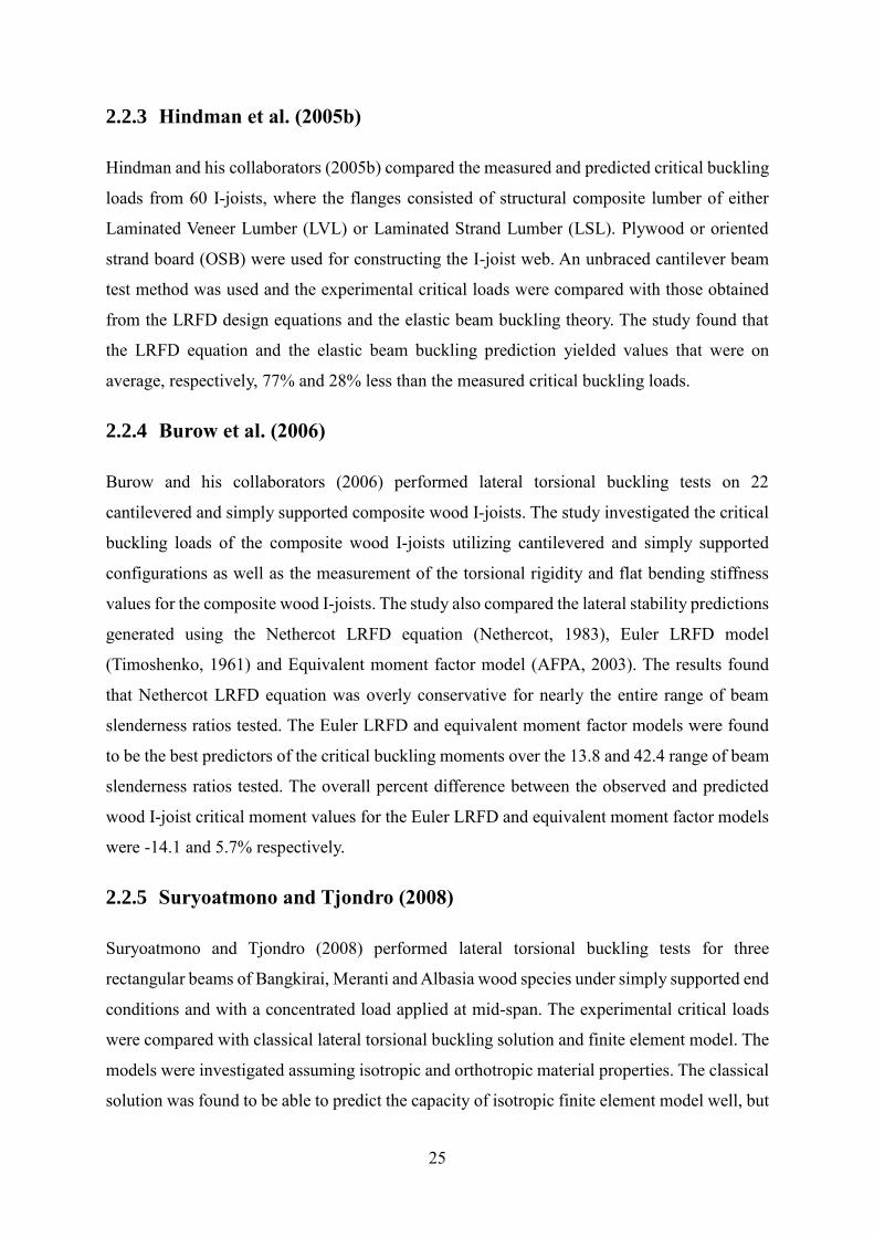
2.2.3 Hindman et al. (2005b)
Hindman and his collaborators (2005b) compared the measured and predicted critical buckling
loads from 60 I-joists, where the flanges consisted of structural composite lumber of either
Laminated Veneer Lumber (LVL) or Laminated Strand Lumber (LSL). Plywood or oriented
strand board (OSB) were used for constructing the I-joist web. An unbraced cantilever beam
test method was used and the experimental critical loads were compared with those obtained
from the LRFD design equations and the elastic beam buckling theory. The study found that
the LRFD equation and the elastic beam buckling prediction yielded values that were on
average, respectively, 77% and 28% less than the measured critical buckling loads.
2.2.4 Burow et al. (2006)
Burow and his collaborators (2006) performed lateral torsional buckling tests on 22
cantilevered and simply supported composite wood I-joists. The study investigated the critical
buckling loads of the composite wood I-joists utilizing cantilevered and simply supported
configurations as well as the measurement of the torsional rigidity and flat bending stiffness
values for the composite wood I-joists. The study also compared the lateral stability predictions
generated using the Nethercot LRFD equation (Nethercot, 1983), Euler LRFD model
(Timoshenko, 1961) and Equivalent moment factor model (AFPA, 2003). The results found
that Nethercot LRFD equation was overly conservative for nearly the entire range of beam
slenderness ratios tested. The Euler LRFD and equivalent moment factor models were found
to be the best predictors of the critical buckling moments over the 13.8 and 42.4 range of beam
slenderness ratios tested. The overall percent difference between the observed and predicted
wood I-joist critical moment values for the Euler LRFD and equivalent moment factor models
were -14.1 and 5.7% respectively.
2.2.5 Suryoatmono and Tjondro (2008)
Suryoatmono and Tjondro (2008) performed lateral torsional buckling tests for three
rectangular beams of Bangkirai, Meranti and Albasia wood species under simply supported end
conditions and with a concentrated load applied at mid-span. The experimental critical loads
were compared with classical lateral torsional buckling solution and finite element model. The
models were investigated assuming isotropic and orthotropic material properties. The classical
solution was found to be able to predict the capacity of isotropic finite element model well, but

26
much higher than orthotropic finite element models. In their comparison with the orthotropic
FEA model with the experimental test, results were observed to agree well for the Albasia
material. The Bangkirai model underestimated the critical load while the Meranti model
overestimated the critical load.
2.2.6 Hindman (2008)
Hindman (2008) performed lateral torsional buckling tests on three simply supported I-joist
members under concentrated load at mid-span. The goals of this study were to determine the
critical buckling load and measure the response of I-joists subjected to the load from a worker
walking on the unbraced I-joists. To achieve the first goal, a static bending test was performed
where three methods were used to determine buckling loads. A novel loading jig was developed
to measure the lateral buckling due to vertical loads. The results of the testing were analyzed
in an attempt to precisely determine the lateral buckling. Lateral buckling tests of unbraced
beams were conducted and the measured loading was observed to include a significant dynamic
load component to cause the lateral torsional buckling.
2.2.7 Bamberg (2009)
Bamberg (2009) studied the behavior of wood I-joists loaded by human test subjects. The goal
of the study was to analyze the relationship between lateral acceleration, displacement and twist
and the brace configuration and stiffness. The study found that the braced configuration did not
exhibit lateral acceleration, while having a lateral displacement and twist. The research also
concluded that an increase in brace stiffness reduced the lateral displacement and twist response.
2.3 Notation for Chapter 2
bC the equivalent moment factor
eC load eccentricity factor
wC the warping constant
d beam depth (mm)
e distance between load position and shear center
E modulus of elasticity (MPa)

27
G shear modulus (MPa)
xI moment of initial in strong axis (mm4)
yI moment of initial in weak axis (mm4)
J Saint Venant torsion constant (mm4)
K Constant based on loading and boundary conditions
L the span of beam between two supports (mm)
eL the effective length of beam (mm)
uL the unbraced length of beam (mm)
1M minimum end moment
2M maximum end moment
AM value of moment in one quarter point between two lateral bracing
BM value of moment in two quarter point between two lateral bracing
CM value of moment in three quarter point between two lateral bracing
crM critical moment of beam
1eM stabilization moment
2eM destabilization moment
maxM maximum moment along the span between two lateral bracing points
uM the critical moment of simply supported beam under constant moment
P Applied load at mid-span
r 1 y xI I
2.4 References
[1] Timoshenko, S. (1961). Theory of Elastic Stability. Second Edition. McGraw-Hill Book Co.
[2] Hooley, R. F. and Madsen, B. (1964). Lateral Buckling of Glued Laminated Beams, Journal

28
of Structural Engineering Division, ASCE, Vol. 90, No. ST3, pp. 201-303.
[3] Galambos, T. V. and Surovek, A.E. (2008). Structural Stability of Steel: Concepts and
Applications for Structural Engineers. John Wiley & Sons, Inc., Hoboken, New Jersey.
[4] American Forest and Paper Association. (2003). Technical Report 14: Designing for lateral-
torsional stability in wood members. Washington, D.C.
[5] American Forest and Paper Association. (2005). DES 140: Designing for Lateral-Torsional
Stability in Wood Members. Washington, D.C.
[6] American Institute of Steel Construction, Inc. (1999). Load and Resistance Factor Design
Specification for Structural Steel Buildings, AISC Manual of Steel Construction, Second
Edition
[7] Kirby, P. A. and Nethercot, D. A. (1979). Design for Structural Stability. Constrado
Monographs, Granada Publishing, Suffolk, UK.
[8] Canadian Standards Association. (2009). CSA standards O86-09, Engineering design in
wood, Mississauga, Ontario, Canada.
[9] Bradford K. & Douglas, P.E. (2006). Design for Lateral-Torsional Stability in Wood
Members. American Forest & Paper Association, Washington, DC, USA.
[10] Filler, J. (2012). Calculating the Beam Stability Factor for a Continuous Timber Beam.
http://voices.yahoo.com/calculating-beam-stability-factor-continuous-
11676794.html?cat=15
[11] Martinelli, E. (2012). Stability of Structures. Department of Civil Engineering, University
of Salerno, Italy, http://www.enzomartinelli.eu/MaterialeDidattico/stabilita/week04.pdf
[12] Hindman D. P., Harvey, H. B. and Janowiak, J. J. (2005a). Measurement and Prediction
of Lateral Torsional Buckling Loads of Composite Wood Materials: Rectangular Section.
Forest Products Journal, Vol. 55, No. 9, pp 42-47.
[13] Hindman D. P., Harvey, H. B. and Janowiak, J. J. (2005b). Measurement and Prediction
of Lateral Torsional Buckling Loads of Composite Wood Materials: I-joist sections. Forest
Products Journal, Vol. 55, No. 10, pp 43-48.

29
[14] Burow, J. R., Manbeck, H. B. and Janowiak, J. J. (2006). Lateral Stability of Composite
Wood I-joists under Concentrated-load Bending. American Society of Agricultural and
Biological Engineers, Vol. 49, pp 1867-1880.
[15] Nethercot, D. A. (1983). Elastic Lateral Buckling of Beams, in Beams and Beam Columns:
Stability in Strength.R. Narayanan, ed. Barking, Essex, U.K.: Applied Science Publishers
[16] Suryoatmono B. and Tjondro A. (2008). Lateral-torsional Buckling of Orthotropic
Rectangular Section beams. Department of Civil Engineering, Parahyangan Catholic
University, Bandung, Indonesia.
[17] Hindman D.P. (2008). Lateral Buckling of I-joist. Department of Wood Science and Forest
Products, Virginia Tech Blacksburg, VA, USA
[18] Bamberg, C. R. (2009). Lateral Movement of Unbraced Wood Composite I-joists Exposed
to Dynamic Walking Loads. M.A.Sc thesis, Virginia Polytechnic Institute and State
University, Blacksburg, Virginia, USA.

30
Chapter 3
Sensitivity Analysis
3.1 General
This chapter aims at conducting a sensitivity analysis of the mechanical properties on the
critical moment capacity of a wooden beam of typical dimensions. According to CSA Standard
O86-09 (CSA, 2009), the capacity of the beam is dictated by lateral torsional buckling due to
lateral stability factor which is equal or less than 1.
Consider a simply supported beam with 80×600 mm cross-section and 5000 mm span (Glued
laminated timber). Beam material properties are Pine lodgepole (Table 3.1). The beam is
assumed to be subjected to a uniform moment. The lateral torsional buckling capacity of the
beam based on a 3D FEA model will be compared to that based on the classical solution. This
will be followed by a sensitivity analysis on a study on the effect of the constitutive properties
on the lateral torsional buckling resistance of the beam.
Table 3.1 Mechanical properties of Pine lodgepole glue-laminated beam (CSA, 2009) (FPL,
2010)
Parameter Value
Modulus of elasticity in the longitudinal direction LE (MPa) 10300
Modulus of elasticity in the tangential direction TE (MPa) 700
Modulus of elasticity in the radial direction RE (MPa) 700
Shear modulus about longitudinal and radial direction LRG (MPa) 474
Shear modulus about longitudinal and tangential direction LTG (MPa) 474
Shear modulus about radial and tangential direction RTG (MPa) 51.5
Poisson’s ratios along longitudinal and radial direction LR 0.347
Poisson’s ratios along longitudinal and tangential direction LT 0.347
Poisson’s ratios along radial and tangential direction RT 0.469

31
3.2 Model Description
3.2.1 Introduction
As discussed in the Introduction and Literature review sections, wood is an anisotropic material
but can generally be considered as an orthotropic material. On a cube taken from a wooden
beam which includes three faces: the L face is perpendicular to the longitudinal direction, the
R face is perpendicular to the radial direction and the T face is perpendicular to the tangential
direction, as shown in Figure 3.1.
Figure 3.1 The Radial and tangential faces of a cube wooden beam
These three faces correspond to the modulus of elasticity ( LE , TE and RE ) along the
longitudinal, tangential and radial direction, respectively. On each face, there are two Poisson’s
ratios (LTv and LRv ) and two shear moduli ( LTG and LRG ) about the longitudinal-tangential
direction and longitudinal-radial direction, respectively, and one Poisson’s ratio (RTv ) and one
shear modulus ( RTG ) about radial and tangential direction. However, the difference between
the properties in the radial and tangential direction can be considered insignificant. Therefore,
T RE E , LT LRv v and LT LRG G . In order to determine the effect of constitutive parameters
on the lateral torsional buckling capacity of a beam, a 3D finite element eigenvalue buckling
analysis is conducted, the three principle axes of the model are shown in Figure 3.2. The effect
of various material properties on the critical moment was systematically investigated by
varying the magnitude of constitutive parameters.

32
Figure 3.2 The three principal axes
3.2.2 The Element Type and Mesh of Model
The C3D8 eight-noded brick element from the ABAQUS library of elements was used to model
the beam (Figure 3.3). The C3D8 element has 8 nodes at the corners and 24 degrees of freedom
(three translations at each node) (Simulia, 2011).
Figure 3.3 C3D8 Element
The finite element model was developed to investigate the lateral torsional buckling capacity
of Pine lodgepole Glued-laminated beams, the beams cross-sections were 80 mm in width, by
600 mm in depth and 5000 mm in span. The dimensions were selected specifically to ensure
that elastic lateral torsional buckling takes place prior to material failure and are thus the beam
capacity and are independent of the strength properties of beam material. In order to ensure the
accuracy of the model, the aspect ratio for each element should be as close as possible to unity.

33
Also, for computational efficiency, the element dimension in the longitudinal direction can be
twice its width or depth. A mesh sensitivity analysis was conducted by increasing the mesh
until no significant change was observed in the critical load. The critical load remained stable
when there were 8 elements taken along the section width 1 8n , 60 elements along the section
depth 2 60n and 250 elements along the span 3 250n , as shown in Figure 3.4. Therefore,
the element dimensions were 10 mm ×10 mm × 20 mm in length (Figure 3.4).
Figure 3.4 Mesh of model
3.2.3 Eigenvalue Analysis
Eigenvalue buckling analysis is a linear perturbation procedure to estimate the critical loads by
solving the system of equation, as shown in Equation (3.1):
0 0i G iK K v (3.1)
where 0K is the elastic stiffness matrix with respect to the base state, GK is the geometric
matrix, i represent the eigenvalues, corresponding to the buckling mode shapes M
iv . For n
degrees of freedom, Equation (3.1) has up to n Eigen pairs i , iv . The lowest positive
eigenvalue among all Eigen value provides the critical loads.
3.2.4 Mechanical Material Properties
The mechanical material properties were taken as those for Pine lodgepole glue-laminated

34
beam. The mean properties as reported in the CSA O86-09 (CSA, 2009) and Wood handbook
(FPL, 2010) are provided in Table 3.1, assuming the properties in the radial direction are
identical to those in tangential direction. These will be taken for adopted for the FEA model of
reference case.
3.2.5 Boundary Conditions
The beam is assumed to be simply supported at both ends relative to the strong axis bending,
weak axis bending, and twist. This includes two types of constraints:
a) Those related to displacements within the plane of the cross-section, a set of restraints are
enforced on the horizontal (AB and A’B’) and vertical lines (CD and C’D’) passing through
the centroid (Figure. 3.5). Degrees of freedom along the transverse direction were restrained at
AB and A’B’, degree of freedom along the lateral direction was restrained at CD and C’D’.
b) Those related to longitudinal displacement on the centroid of cross-section. At one end of
beam (Figure 3.5), degree of freedom along the longitudinal, transverse, lateral direction were
restrained on centroid of the cross-section, at the other end, only the degree of freedom along
the tangential and radial directions were restrained on the centroid of cross-section. The above
explanation simulates the simply supports of the beam, at both ends, the lateral and transverse
displacements were restrained but free to rotate about strong and weak axis, at one end, the
displacement along the longitudinal direction was restrained but the other end is free to move
along the longitudinal direction.

35
(a)
(b)
(c)
(d)
Figure 3.5 Boundary conditions (all crossed arrows denote restrained degrees of freedoms
that are restrained)
(a) sketch of left end, (b) sketch of right end, (c) left end in ABAQUS model, and (d) right end
in ABAQUS model
3.2.6 Constraints Related to the Longitudinal Degrees of Freedom
In line with the longitudinal displacement w for a generic point ,x y at both beam ends

36
( 0el and l ) is given by
, , xe e e e ew l y l l x l y l xy (3.2)
el is the displacement of the centre of the cross-section along the longitudinal direction,
( )el is the displacement along x axis (along the lateral direction), ( )el is the displacement
along y axis (along the tangential direction), ( )el is the rotation about the longitudinal
direction.
Applying Equation (3.2) at all 4 corner points with coordinates , 1, 2,3, 4i ix y i , the
longitudinal displacements of corners of end cross-section are given by
1 1 1 1 1
2 2 2 2 2
3 3 3 3 3
4 4 4 4 4
1
1
1 ( )
1 ( )
e
e
e
e
w x y x y l
w x y x y l
w x y x y l
w x y x y l
(3.3)
Solving Equation (3.3), for vector ( ) ( )T
e e e el l l l , results in
1
1 1 1 1 1
2 2 2 2 2
3 3 3 3 3
4 4 4 4 4
1
1
1( )
1( )
e
e
e
e
x y x y wl
x y x y wl
x y x y wl
x y x y wl
(3.4)
From Equation (3.4) into (3.2), gives
1
1 1 1 1 1
2 2 2 2 2
3 3 3 3 3
4 4 4 4 4
1
1, , 1 0
1
1
T
e
x y x y w
x y x y ww l x y x y xy
x y x y w
x y x y w
(3.5)
Equation (3.5) provides the longitudinal displacement w at any generic point , ,el x y on end
el in terms of the longitudinal displacements of corner points. The above constraint is then
enforced in the ABAQUS model on all nodal points of the end cross-sections using the

37
Equation feature of ABAQUS. The procedure is shown in Figure 3.6 for node (x,y) = (20,30).
Equation (3.5) provides the constraint
1 2 3 4, , 0.4125 0.1375 0.1125 0.3375 0ew l x y w w w w . The first coefficient corresponds
to the node at which the constraint is enforced and the rest of the coefficients are those of the
four corner points.
Figure 3.6 Edit equation constraint of node (x,y) =(20,30) (Simulia, 2011)
3.2.7 Load Application
The beam is subjected to equal end moments. This is achieved by applying four concentrated
longitudinal forces P applied at the corners of the end cross-sections along the longitudinal
direction, as shown in Figure 3.7. It is evident that the applied forces have zero longitudinal
resultant, weak axis moments, and bi-moments. The resultant strong axis moment is equal to
4 ( 2) 2p d pd .

38
(a)
(b)
(c)
(d)
Figure 3.7 Load Application in the FEA model
(a) at the left end of the beam, (b) at the right end of the beam,
(c) at the left end in model, (d) at the right end in model
3.3 Comparison with Classical LTB Solution
The critical moment uM for a simply supported beam subject to uniform bending as given by
the classical solution is
2
Lu L T y w
u u
y
EM E I G J I C
L L
(3.6)
on which uL is the unbraced length of beam, LE is modulus of elasticity along the longitudinal

39
direction. Since the shear modulus about longitudinal and tangential direction LTG is assumed
to have the same magnitude as the shear modulus about longitudinal and radial direction LRG ,
shear modulus about transverse direction TG is used to replace the value of LTG and LRG . J
is Saint Venant Torsion constant, yI is moment of inertia in weak axis and wC is warping
constant.
For a rectangular section of width b and depth d , the weak axis moment of inertia is
3 /12yI db . The Saint Venant Torsional constant is 3J kdb , where k is a constant
depending on the aspect ratio /d b . For a cross-section aspect ratio of 600 / 80 7.5d b and
given that / 60.299
d bk
and / 10
0.312d b
k
(Ugural & Fenster, 1975), through linear
interpolation, one obtains / 100.312
d bk
. The warping constant wC for a rectangular section
is given by
3 32 2
2 2 2
2 2
( )144
b d
w
b d
b dC xy dA x y dxdy
(3.7)
In summary, the section properties are7 42.56 10yI mm ,
11 67.68 10wC mm ,
7 69.34 10J mm . When applying Equation (3.6) to an orthotropic material, the modulus of
elasticity in the longitudinal direction 10,300LE MPa and the shear modulus about
transverse is taken as 474TG MPa .
For the 5 m span considered, the critical moment as obtained by Equation (3.6) is 70.2 kNm
while that predicted by FEA is 67.9 kNm. This corresponds to a ratio of FEA to classical
solution of 0.967. Figure 3.8 shows the buckled configuration for a beam subjected to uniform
moment as predicted by the FEA model.

40
Figure 3.8 ABAQUS model of lateral torsional buckling
3.4 Sensitivity Analysis
In addition to the reference case investigated under Section 3.2 for which 10300L refE MPa ,
700t refE MPa , 474T refG MPa , 0.347T refv , 51.5RT refG MPa and 0.469RT refv .
12 sensitivity runs were conducted. In each of the runs, five of the six constitutive constants
were kept unchanged and the value of the remaining constitutive constant was changed, once
by a factor of 1.5 and another time by a factor of 0.5. The ratio of the resulting critical moment
to the reference critical moment is then provided. The resulting critical moments and ratio
between the resulting critical moments and that based on the reference case are shown in Table
3.2:

41
Table 3.2 Effect of Constitutive parameters on critical moments as predicted by FEA
Case e
L
L r f
E
E
T
T ref
G
G
t
t ref
E
E
T
T ref
RT
RT ref
RT
RT ref
G
G
crM
(MPa)
cr
cr ref
M
M
Reference
case 1 1 1 1 1 1 67.9 1.00
1 1.5 1 1 1 1 1 84.4 1.24
2 0.5 1 1 1 1 1 47.3 0.697
3 1 1.5 1 1 1 1 81.6 1.20
4 1 0.5 1 1 1 1 49.9 0.735
5 1 1 1.5 1 1 1 68.0 1.00
6 1 1 0.5 1 1 1 67.8 1.00
7 1 1 1 1.5 1 1 67.9 1.00
8 1 1 1 0.5 1 1 67.9 1.00
9 1 1 1 1 1.5 1 67.9 1.00
10 1 1 1 1 0.5 1 67.9 1.00
11 1 1 1 1 1 1.5 68.3 1.01
12 1 1 1 1 1 0.5 67.1 0.988
Note: Since the difference between the properties in the radial and tangential direction can be
considered insignificant and assumed to be the same value in analysis, the modulus of elasticity
about transverse tE R T tE E E and the Poisson’s ratio about transverse Tv are used
to replace the corresponding properties in the radial and tangential direction.
Figures 3.9 shows the normalized critical moment versus the normalized longitudinal Young
Modulus as predicted by FEA and that based on the classical solution. Also, Figure 3.10 shows
the normalized critical normalized critical moment versus the normalized longitudinal shear
modulus as predicted by FEA and that based the classical solution.

42
Figure 3.9 The comparison of Mcr/Mcr-ref with EL/EL-ref
Figure 3.10 The comparison of Mcr/Mcr-ref with GT/GT-ref
The sensitivity results (Table 3.2) show that the critical moments are significantly affected by
the modulus of elasticity ( )LE in the longitudinal direction, and the transverse shear modulus
( )TG . Thus, an accurate determination of these constants is needed. This will be the scope of
Chapter 4 and 5. In contrast, the effect of the modulus of elasticity ( )tE , Poisson’s ratios ( )T ,
( )RT and shear modulus ( )RTG have a negligible effect on critical moment. An accurate
determination of these material constants is not needed.
0
0.5
1
1.5
2
2.5
0 0.5 1 1.5 2
Mcr
/Mcr
-ref
EL/EL-ref
ABAQUS results
Classical LTB solution
0
0.5
1
1.5
2
2.5
0 0.5 1 1.5
Mcr/M
cr-r
ef
GT/GT-ref
ABAQUS results
Classical LTB solution

43
3.5 Notation for Chapter 3
b beam width (mm)
wC the warping constant (mm6)
d beam depth (mm)
LE modulus of elasticity in the longitudinal direction (MPa)
TE modulus of elasticity in the tangential direction (MPa)
tE modulus of elasticity about transverse (MPa)
RE modulus of elasticity in the radial direction (MPa)
LTG shear modulus about longitudinal and tangential direction (MPa)
LRG shear modulus about longitudinal and radial direction (MPa)
TG shear modulus about transverse (MPa)
yI moment of initial in weak axis (mm4)
J Saint Venant torsion constant (mm4)
k constant depending on the aspect ratio /d b
0K elastic stiffness matrix with respect to the base state
GK geometric matrix
p concentrated load applied on the corner of cross-section
w longitudinal displacement
( )el rotation about longitudinal direction
el displacement of centre of cross-section along the longitudinal direction
( )el displacement along transverse axis
i eigenvalues
M
iv buckling mode shapes
44
LR Poisson’s ratios about longitudinal and radial direction
LT Poisson’s ratios about longitudinal and tangential direction
RT Poisson’s ratios about radial and tangential direction
T Poisson’s ratios about transverse
( )el displacement along lateral axis
3.6 References
[1] Canadian Standards Association. (2009). CSA standards O86-09, Engineering design in
wood, Mississauga, Ontario, Canada.
[2] Forest Products Labratory. (2010): Wood Handbook-Wood as an Engineering Material.
Madison, USA.
[3] Simulia. (2011), ABAQUS analysis user’s manual (Version 6.11), Dassault Systemes.
[4] Uqural, A.C. and Fenster, S.K. (1975). Advanced Strength and Applied Elasticity,
American Elsevier Pub Co, New York, USA.

45
Chapter 4
Experimental Program
4.1 Introduction
As discussed in the Sensitivity analysis section (Chapter 3), the lateral torsional buckling is
only dependent on the weak direction modulus of elasticity along the longitudinal direction
( LE ) and shear modulus about the transverse direction ( TG ). All other parameters in lateral
torsional buckling analysis are determined by the geometry of beam. As wood can be
considered an orthotropic material, LE and TG values are direction dependent. The modulus
of elasticity is that achieved from the lateral bending stiffness, which introduces strain parallel
to the grains. The value of TG is more complex to estimate because it depends on how the piece
of wood is cut, as seen in Figure 1.2 in the Introduction section (Chapter 1) and how the wood
element is installed.
Therefore, depending on the orientation of the cut, the value of TG would be that of LRG or
LTG . The value of TG will, in reality, likely be a combination of the two values, and is best
determined experimentally. Values in the literature (FPL, 2010) of LRG and LTG do not have
high variability but they could introduce a significant error into the calculations. The effect of
such difference was investigated in Chapter 3.
The testing program involved the two generic materials used in the CSA O86 standard (CSA,
2009), namely lumber and glue-laminated timber. The provisions in the design code are
provided in the glulam design clause but they are also applicable to lumber. To the author’s
knowledge, few reported testing has ever been done on lumber products to validate the general
theory for lateral torsional buckling. Therefore, this study’s emphasis for the full scale tests
was on lumber joists.
Due to its dimensional stability and precise manufacturing, the variation in dimension of glue-
laminated timber members is usually found to be very small. However, this consistency cannot
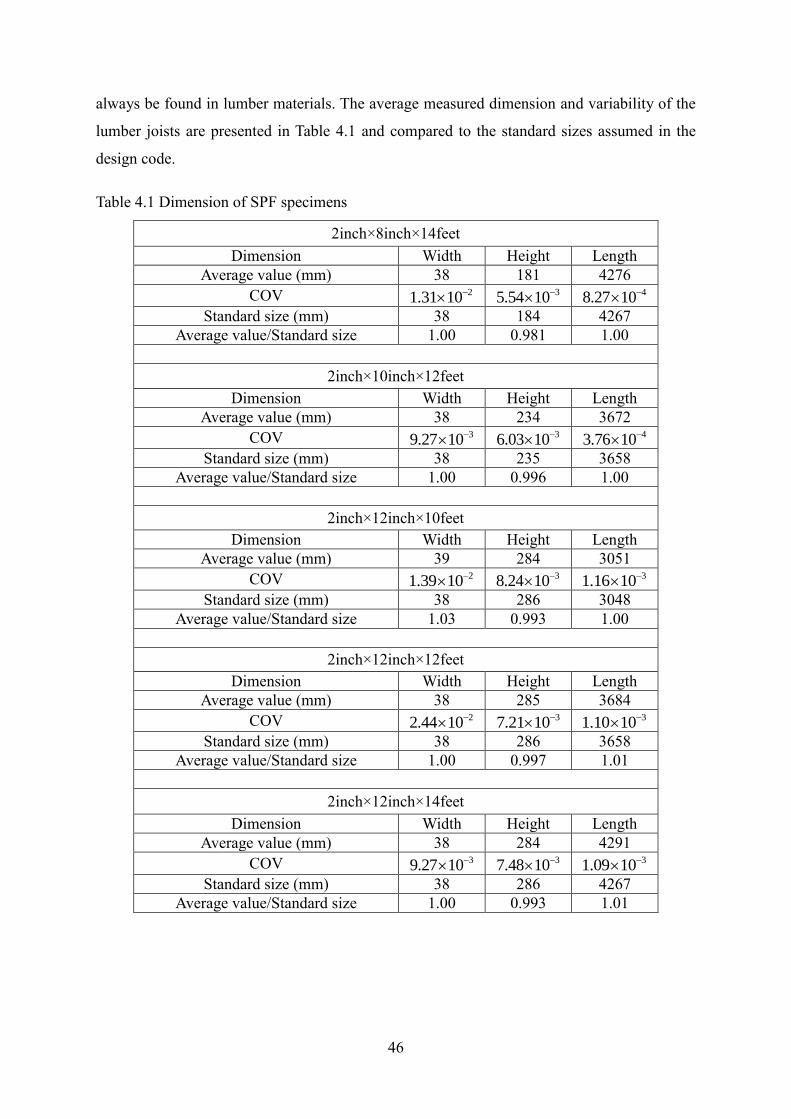
46
always be found in lumber materials. The average measured dimension and variability of the
lumber joists are presented in Table 4.1 and compared to the standard sizes assumed in the
design code.
Table 4.1 Dimension of SPF specimens
2inch×8inch×14feet
Dimension Width Height Length
Average value (mm) 38 181 4276
COV 21.31 10 35.54 10 48.27 10
Standard size (mm) 38 184 4267
Average value/Standard size 1.00 0.981 1.00
2inch×10inch×12feet
Dimension Width Height Length
Average value (mm) 38 234 3672
COV 39.27 10 36.03 10 43.76 10
Standard size (mm) 38 235 3658
Average value/Standard size 1.00 0.996 1.00
2inch×12inch×10feet
Dimension Width Height Length
Average value (mm) 39 284 3051
COV 21.39 10 38.24 10 31.16 10
Standard size (mm) 38 286 3048
Average value/Standard size 1.03 0.993 1.00
2inch×12inch×12feet
Dimension Width Height Length
Average value (mm) 38 285 3684
COV 22.44 10 37.21 10 31.10 10
Standard size (mm) 38 286 3658
Average value/Standard size 1.00 0.997 1.01
2inch×12inch×14feet
Dimension Width Height Length
Average value (mm) 38 284 4291
COV 39.27 10 37.48 10 31.09 10
Standard size (mm) 38 286 4267
Average value/Standard size 1.00 0.993 1.01

47
4.2 Torsional Test to Determine the Shear Modulus
Tests to determine the shear modulus were conducted in accordance with the ASTM D198
(2009) standard. Ten (10) glulam and thirty-eight (38) lumber specimens were tested. All
glulam timber beams consisted of 20f-E bending grade and had the dimensions of 80 mm in
width and 228 mm depth. Each member consisted of a single lamination in width and was
connected by finger joints in length, as shown in Figure 4.1.
(a)
(b)
Figure 4.1 The glued laminated timber for torsional testing
(a) Laminations of glulam beam and (b) Finger joint of lamination
All the lumber joists were Spruce-Pine-Fir (SPF), No.1/No.2 grade. The geometries included
2×8 inch nominal dimension with 14 feet in length, 2×10 inch with 12 feet length, 2×12 inch
with 10, 12, and 14 feet lengths. The specimens were conditioned to a moisture content of 12%
on average. The maximum moisture content measured was 16.1%.
4.2.1 Torsion Test Set-up
The glulam test specimens were clamped symmetrically about the longitudinal axis by two
steel clamps at each end. The load was applied by a hydraulic jack on the top of the wide flange
steel bracket. The magnitude of the applied load was measured using a load cell located
between the jack and the steel bracket. The load application points and the support were made
from beveled wood cross section in order to allow for free rotation about the longitudinal axis

48
of the specimens. The distance between the contact points of bearing and the center of the
cross-section was 400 mm and the distance between the two clamps was 2000 mm. Due to the
symmetry in the setup, the specimens received a uniform coupled torsional moment at each
end. Based on the requirement of ASTM 198 (2009), the total length of specimen (and distance
between clamps) should be at least eight times greater than the larger cross-sectional dimension.
Figure 4.2 and 4.3 show a schematic and laboratory test set-up, respectively, of the glulam
torsion tests.
The only differences between the glulam and lumber torsional test were that for lumber the
brackets were made out of wood, to reduce the weight on the test specimens and the distance
between the clamps was 2600 mm. Figure 4.4 presents the laboratory test set-up for the SPF
joists.

49
(a)
(b)
Figure 4.2 Schematic of torsion test set-up for glulam
(a) Two dimensional view of the torsion test set-up, (b) Three dimensional view of torsion
test setup

50
Figure 4.3 Laboratory torsion test of glulam
Figure 4.4 Laboratory torsion test of SPF
Hydraulic jack
Load cell
Steel bracket
Specimen
Hydraulic jack
Load cell
Wood bracket
Specimen

51
4.2.2 Determining the Angle of Twist
To obtain the angle of twist, the displacements at the top and bottom of the beam at each end
near the clamps were measured using wire gauges with a 600 mm stroke. A knee-wall
constructed near the test setup was used as a reference point for the displacement measurements.
Figure 4.5 shows the connection between wire gauge and the test specimen. Inclinometers were
also used to measure the angle of twist. They were installed on the top of the test specimens as
close as possible to the clamps, as shown in Figure 4.6.
(a)
(b)
Figure 4.5 The connection between wire gauge to Glulam beam
(a) Wire gauge connect to the glulam, and (b) End of wire gauge were fixed on the frame
Figure 4.6 The installation of inclinometer in SPF
Wire gauge
Inclinomete
r
Wire gauge

52
4.3 Bending Test Set-up
Seventeen (17) glulam and thirty-six (36) lumber specimens were tested in the weak-direction
bending in accordance with the ASTM D198 standard (ASTM, 2009) to obtain their modulus
of elasticity ( LE ). The load application points were located at the third point of the clear span.
No bracing of the beams was required as out of plane buckling could not occur. Since the
direction of lateral torsional buckling in a beam is random, the LE was measured on both sides
of the specimens and the average values were used in calculating the critical value in the
capacity calculation. The applied load was measured using a load cell which was located
between the hydraulic jack and load transfer device. The mid-span deflection was measured
using a wire gauge with the lab strong floor as reference. The set-up for bending test is shown
in Figures 4.7 and 4.8.

53
Hydraulic jack
Load transfer device
Wire gauge
Load cell
677.3mm 677.3mm 677.3mm
2032.0mm
Hydraulic jack
Load cell
Load transfer device
Test specimen
(a) (b)
Figure 4.7 Schematic drawing of the weak axis bending test set-up
(a) Profile, and (b) Side

54
Figure 4.8 The set-up of weak axis bending for SPF
4.4 Full-scale Lateral Torsional Buckling Test Set-up
As mentioned earlier, the focus of the full scale lateral torsional buckling experimental
testing was on lumber due to the lack of data in this area. The main objective was to
demonstrate the validity of classical lateral torsional solution for orthotropic wood
material. Eighteen test samples with aspect ratios that would yield failure in the elastic
region, according to Canadian timber design code provisions (CSA, 2009), were
selected for the full scale lateral torsional buckling tests. The slenderness ratios BC
were calculated to 29.4, 30.7, and 36.6 for specimens 2”×8”×14’, 2”×10”×12’, and
2”×12”×14’, respectively (Table 4.2). KC , in Table 4.2, is equal to
2(0.97 ) ( )SE T B b XEK K C F K , and it constitutes the point beyond ( BC > KC ) which the
element is in elastic region, where bF is specified strength in bending, SEK is the
service condition factor of modulus of elasticity, TK is treatment factor, XK is
curvature factor, and the value of SEK , TK and XK are equal to 1.

55
Table 4.2 Slenderness of the tested specimens
Beam sectional
dimension (inch)
Clear
span(mm)
Specimen
amount
Slenderness
ratio KC
2×8 4200 5 29.4 27.9
2×10 3600 6 30.7 27.9
2×12 4200 7 36.6 27.9
4.4.1 Boundary Conditions
A very important aspect of the full scale lateral torsional buckling test setup is the
boundary support conditions. The boundary conditions assumed in the classical solution
to the lateral torsional buckling problem are the end cross-sections are free to rotate
about the strong and weak axis but restrained to move along the tangential and lateral
direction. The boundary supports chosen in the experimental program attempted to
mimic as much as possible these assumptions. The supports were constructed using two
steel rods which were welded to the bottom plate and fastened with one piece of HSS
steel on top to prevent rotation of the specimen about the longitudinal direction and
buckling laterally at each end. The end supports were made to rotate about the weak
axis of end cross-section. A hole with 3/4” in diameter was drilled into the wood support
and a steel shaft with same diameter was welded underneath the end support. A thrust
bearing was placed between the steel rod and hole of wood support, as shown in Figure
4.9. Since the steel rod and hole had the same diameter, the support is free to rotate but
braced from buckling laterally.
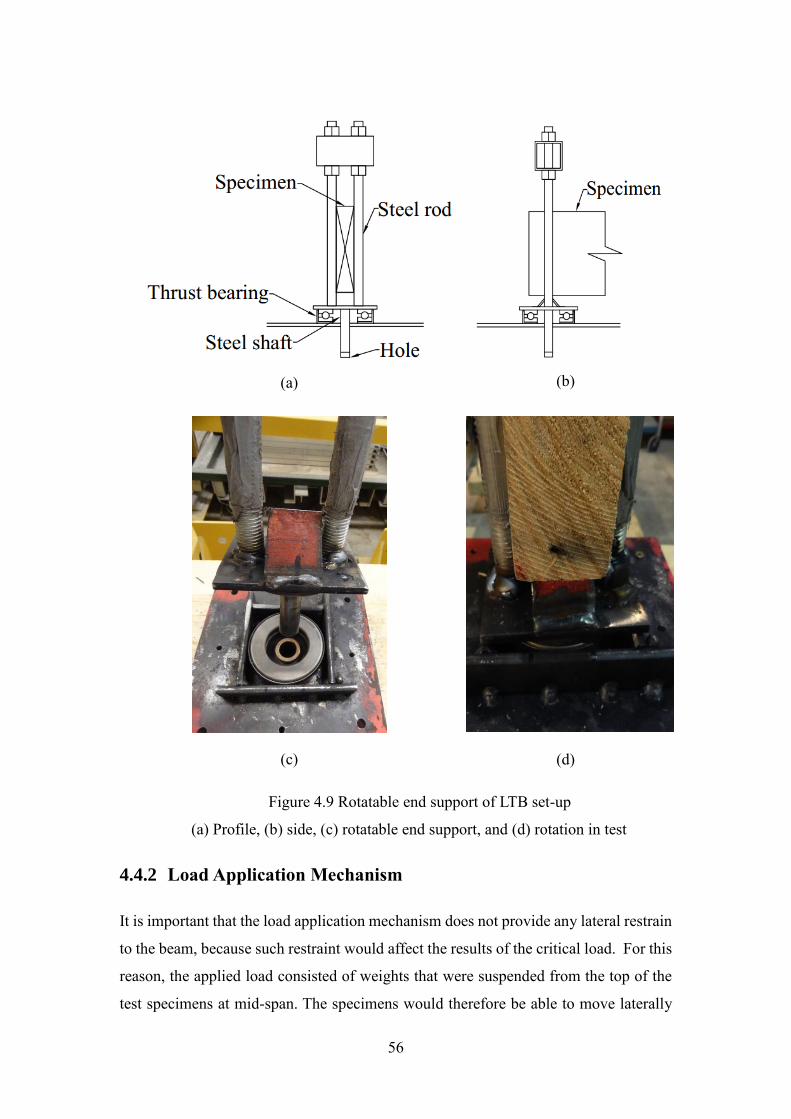
56
(a)
(b)
(c)
(d)
Figure 4.9 Rotatable end support of LTB set-up
(a) Profile, (b) side, (c) rotatable end support, and (d) rotation in test
4.4.2 Load Application Mechanism
It is important that the load application mechanism does not provide any lateral restrain
to the beam, because such restraint would affect the results of the critical load. For this
reason, the applied load consisted of weights that were suspended from the top of the
test specimens at mid-span. The specimens would therefore be able to move laterally

57
without any additional restraints. As shown in Figure 4.10, the loading frame consisted
of three parts: A steel HSS load transfer beam, a wood base to support the weight and a
steel rod that allows rotation of the frame when the beam starts deflecting laterally
(a)
(b)
(c)
Figure 4.10 Connection between load frame and specimen
(a) Profile, (b) Side, and (c) Load application frame
4.4.3 Instrumentation
The angle of twist and lateral deflection at mid-span were measured by two wire gauges,

58
the lateral displacement of middle height was the average value of two wire gauges
(located at the top and bottom of mid-span), the twist was calculated by the difference
of top and bottom lateral displacement of mid-span, and the vertical deflection of
middle span was measured using a wire gauge, which was located on the mid-height at
mid-span. A schematic drawing and a picture of the set-up are presented in Figure 4.11
and 4.12.

59
Specimen
Load frame
Rotatable support
Weights2inch
8inch
(10inch)
(12inch)Wire gauge point
Rotatable support
Specimen
(a) (b)
Figure 4.11 Schematic Lateral torsional buckling set-up
(a) Profile, and (b) side

60
Figure 4.12 The set-up of lateral torsional buckling test

61
4.5 Notation for Chapter 4
BC slenderness ratios
E modulus of elasticity (MPa)
LE modulus of elasticity in the longitudinal direction (MPa)
bF specified strength in bending (MPa)
LRG shear modulus about longitudinal and radial direction (MPa)
LTG shear modulus about longitudinal and tangential direction (MPa)
TG shear modulus about transverse (MPa)
SEK service condition factor of modulus of elasticity
TK treatment factor
XK curvature factor
4.6 References
[1] Forest Products Labratory. (2010). Wood Handbook-Wood as an Engineering Material.
Madison, USA.
[2] Canadian Standards Association. (2009). CSA standards O86-09, Engineering design in wood,
Mississauga, Ontario, Canada.
[3] ASTM Standard D198. (2009). Standard Test Method of Static Tests of Lumber in Structural
Sizes. Philadelphia, Pa.

62
Chapter 5
Experimental Results
5.1 General
The experimental results from the torsion, bending and full-scale lateral torsional buckling tests
are presented in this chapter. The chapter also presents the failure characteristics observed in the
torsional and lateral torsional buckling tests.
5.2 Torsional Test Results
5.2.1 Calculation Method
A torsional test setup was constructed and tests were conducted in accordance with the ASTM
D198 (2009) standard. The value of the shear modulus TG for each test specimen was calculated
using Equation (5.1) (Hibbeler, 2011):
i
T
TL
JG (5.1)
Where T is the applied torque force, iL is the distance between inclinometers, TG is the shear
modulus about the transverse direction, is the angle of twist, J is the Saint Venant Torsional
constant.
5.2.2 Torsional Test to Failure
There are very few studies that have looked at wood failure in torsion both in terms of failure
capacity and failure modes. Torsion is expected to be very low in wood and is therefore typically
ignored and load causing torsional stresses are usually avoided in structural design and detailing.

63
In order to estimate a level of stress required to obtain the torque force and angle of twist
relationships while still remaining in the linear elastic region, destructive tests were conducted on
both glulam beams and lumber joists to determine the failure load and failure modes.
As shown in Figure 5.1, torsional shear stressed cause fracture to occur along the fibers and
multiple such cracks were observed on the side face of the beam. The load-angle of twist curves
were almost linear until failure, as seen in Figure 5.2. This trend is consistent with those found in
the literature (Yang, 2012, Khokhar, 2012).
(a)
(b)
Figure 5.1 Failure of torsion test
(a) Failure of Glulam beam in torsion, and (b) Failure of SPF beam in torsion

64
Figure 5.2 Force-twisting angle plot until failure of Glulam beam
Based on the test results, it was deemed appropriate to load the test specimens up to approximately
40% of the ultimate load, to ensure that the specimens were within the linear-elastic region and
that no damage was incurred by the specimens during the loading.
5.2.3 Shear Modulus for Glulam Beams
The average TG value for ten glulam beams tested was 672 MPa with a COV 0.06. The test results
are shown in Table 5.1 and illustrated graphically in Figure 5.3. Such low variability in the test
results is expected for engineered wood products such as glulam beams. Figure 5.4 shows a typical
torque-angle of twist relationship for glulam.
0
500000
1000000
1500000
2000000
2500000
3000000
0 0.05 0.1 0.15 0.2 0.25
Twist angle (radian)
Ap
pli
edto
rqu
e (N
mm
)
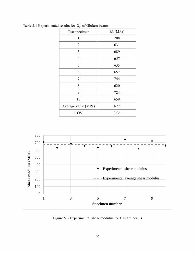
65
Table 5.1 Experimental results for TG of Glulam beams
Test specimen TG (MPa)
1 708
2 631
3 689
4 657
5 635
6 657
7 744
8 620
9 724
10 659
Average value (MPa) 672
COV 0.06
Figure 5.3 Experimental shear modulus for Glulam beams
0
100
200
300
400
500
600
700
800
1 3 5 7 9
Experimental shear modulus
Experimental average shear modulus
Specimen number
Sh
ear
mod
ulu
s (M
Pa)

66
Figure 5.4 Typical torque-twisting angle plot for Glulam specimen
5.2.4 Shear Modulus for Lumber
The TG values obtained from the torsional test for the SPF elements are summarized in Table 5.2.
The average TG of all the specimens tested was 550 MPa, which is slightly lower than that
obtained for glulam. This is expected as the grade of glulam, especially of the outer laminates, is
higher than that of the lumber joists. The COV varied between 0.11 and 0.22, which is also
expected given the variability expected from visually graded lumber joists. This variability is
illustrated graphically in Figure 5.5. The force-twisting angle relationship for the lumber joists was
also linear-elastic, similar to what was observed for glulam.
0
200000
400000
600000
800000
1000000
1200000
0 0.02 0.04 0.06 0.08 0.1
Twisting angle (radian)
Ap
pli
ed t
orq
ue
(Nm
m)

67
Table 5.2 The experimental shear modulus value of SPF beams
Sectional dimension Beam
number k J (×106 mm) TG (MPa)
2”×8”×14’
1 0.289 2.886 501
2 0.289 2.870 614
3 0.288 2.845 558
4 0.289 2.870 548
5 0.288 2.845 705
6 0.287 3.064 540
7 0.289 2.870 808
Average value 610
COV 0.18
2”×10”×12’
1 0.299 3.839 542
2 0.299 3.806 535
3 0.300 3.868 569
4 0.299 3.839 710
5 0.299 3.790 606
6 0.300 3.868 550
7 0.299 4.150 632
8 0.299 3.839 515
Average value 583
COV 0.11

68
Table 5.2: The experimental shear modulus value of SPF beams
Sectional dimension Beam
number k J (×106 mm) TG (MPa)
2”×12”×10’
1 0.303 5.140 447
2 0.304 4.754 470
3 0.303 5.105 482
4 0.304 4.771 536
5 0.303 5.140 457
6 0.303 5.033 650
7 0.304 4.704 414
Average value 494
COV 0.16
2”×12”×12’
1 0.304 4.771 462
2 0.304 4.687 465
3 0.304 5.193 391
4 0.303 5.140 593
5 0.304 4.754 656
6 0.304 4.737 675
7 0.304 4.737 457
8 0.305 4.041 690
Average value 549
COV 0.22

69
Table 5.2: The experimental shear modulus value of SPF beams
Sectional dimension Beam
number k J (×106 mm) TG (MPa)
2”×12”×14’
1 0.304 4.737 451
2 0.304 4.754 521
3 0.303 5.140 479
4 0.304 4.754 515
5 0.304 4.687 442
6 0.304 4.737 720
7 0.304 4.754 537
8 0.303 4.655 471
Average value 517
COV 0.172
Figure 5.5 Experimental shear modulus for SPF beams
0
100
200
300
400
500
600
700
800
900
1 2 3 4 5 6 7 8
Experimental Average Shear Modulus
2inchx8inchx14feet
2inchx10inchx12feet
2inchx12inchx10feet
2inchx12inchx12feet
2inchx12inchx14feet
Specimen Number
Sh
ear
Mod
ulu
s (M
Pa)

70
5.3 Bending Test Results
5.3.1 Determining the Modulus of Elasticity of Glulam Beams about the Weak
Axis
The same glulam beams that were tested non-destructively in torsion and the other seven glulam
specimens with same grade and dimensions were subjected to four-point bending loading to
determine their weak axis modulus of elasticity along the longitudinal direction LE . The end
conditions were pinned and no lateral bracing was deemed necessary due to the low depth to width
aspect ratios of the beams. As mentioned in Chapter 3, due to the uncertainty in the direction of
the buckling, LE of both faces were determined. Table 5.3 summarizes the test results for each
side and the average LE calculated. The average LE of all specimens was 8503 MPa with COV
of 0.07. The experimental results of the 17 Glulam beams are also presented in Figure 5.6.
Table 5.3 The LE values of Glulam beams about weak axis
Beam number surface LE values of
individual side
(MPa)
LE values of
specimen
(MPa)
1 1-a 9613
9826 1-b 10039
2 2-a 8055
8031 2-b 8007
3 3-a 9364
9395 3-b 9427
4 4-a 8302
8158 4-b 8014
5 5-a 8324
8130 5-b 7936
6 6-a 7513
7373 6-b 7232

71
Table 5.3 The LE values of Glulam beams about weak axis
Beam number surface LE values of
individual side
(MPa)
LE values of
specimen
(MPa)
7 7-a 8963
8901 7-b 8839
8 8-a 8475
8721 8-b 8968
9 9-a 8042
8065 9-b 8087
10 10-a 8374
8261 10-b 8147
11 11-a 8449
8572 11-b 8694
12 12-a 8545
8292 12-b 8039
13 13-a 8226
8458 13-b 8691
14 14-a 8511
8669 14-b 8828
15 15-a 8740
8711 15-b 8682
16 16-a 8711
8732 16-b 8754
17 17-a 8397
8251 17-b 8106
Average of all Glulam beams (MPa) 8503
COV 0.07
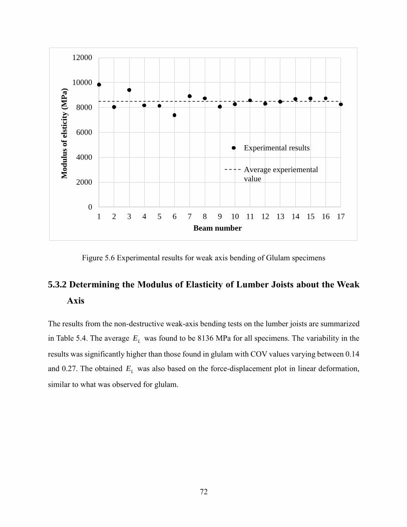
72
Figure 5.6 Experimental results for weak axis bending of Glulam specimens
5.3.2 Determining the Modulus of Elasticity of Lumber Joists about the Weak
Axis
The results from the non-destructive weak-axis bending tests on the lumber joists are summarized
in Table 5.4. The average LE was found to be 8136 MPa for all specimens. The variability in the
results was significantly higher than those found in glulam with COV values varying between 0.14
and 0.27. The obtained LE was also based on the force-displacement plot in linear deformation,
similar to what was observed for glulam.
0
2000
4000
6000
8000
10000
12000
1 2 3 4 5 6 7 8 9 10 11 12 13 14 15 16 17
Experimental results
Average experiemental
value
Beam number
Mod
ulu
s of
elst
icit
y(M
Pa)

73
Table 5.4 The experimental results of weak axis bending tests for SPF specimens
Sectional dimension Beam
number Surface LE values of
individual side (MPa)
LE values of
specimen (MPa)
2”×8”×14’
1 1-a 10333
10434 1-b 10535
2 2-a 8966
9022 2-b 9077
3 3-a 11163
11185 3-b 11207
4 4-a 10269
10111 4-b 9952
5 5-a 7226
7382 5-b 7537
6 6-a 10000
9947 6-b 9894
Average value of SPF beam (MPa) 9680
COV 0.14
2”×10”×12’
1 1-a 11418
11217 1-b 11015
2 2-a 9274
9745 2-b 10215
3 3-a 5575
5563 3-b 5550
4 4-a 9693
9279 4-b 8864
5 5-a 12196
12339 5-b 12482
6 6-a 6337
7619 6-b 8902

74
Table 5.4 The experimental results of weak axis bending tests for SPF specimens
Sectional dimension Beam
number Surface LE values of
individual side (MPa)
LE values of
specimen (MPa)
2”×10”×12’
7 7-a 8416
8092 7-b 7768
8 8-a 9025
9009 8-b 8992
Average value of SPF beam (MPa) 9108
COV 0.23
2”×12”×10’
1 1-a 7395
7057 1-b 6719
2 2-a 8264
8227 2-b 8189
3 3-a 9086
9103 3-b 9120
4 4-a 10415
10339 4-b 10264
5 5-a 5855
6165 5-b 6474
6 6-a 6242
6151 6-b 6059
7 7-a 7906
7706 7-b 7505
Average value of SPF beam (MPa) 7821
COV 0.21
2”×12”×12’
1 1-a 9166
9061 1-b 8956
2 2-a 8495
8459 2-b 8423

75
Table 5.4 The experimental results of weak axis bending tests for SPF specimens
Sectional dimension Beam
number Surface LE values of
individual side (MPa)
LE values of
specimen (MPa)
2”×12”×12’
3 3-a 6794
6932 3-b 7070
4 4-a 3854
3776 4-b 3697
5 5-a 7274
7728 5-b 8182
6 6-a 9262
9305 6-b 9347
7 7-a 6211
6070 7-b 5929
Average value of SPF beam (MPA) 7333
COV 0.265
2”×12”×14’
1 1-a 5976
6668
1-b 7359
2 2-a 6725
7171 2-b 7617
3 3-a 6340
6469 3-b 6598
4 4-a 5654
5960 4-b 6265
5 5-a 7987
7880 5-b 7774
6 6-a 5722
5491 6-b 5261
7 7-a 6544
6364 7-b 6183

76
Table 5.4 The experimental results of weak axis bending tests for SPF specimens
Sectional dimension Beam
number Surface LE values of
individual side (MPa)
LE values of
specimen (MPa)
2”×12”×14’
8 8-a 9959
9876 8-b 9792
Average value of SPF beam (MPA) 6985
COV 0.197
5.4 Results from the Full-scale Lateral Torsional Buckling Tests
Figures 5.7, 5.8 and 5.9 show typical force-lateral displacement, force-vertical displacement and
force-twist angle plots of the specimens at mid-span. It can be seen that when the applied load
approached to the critical load, a slight increase in load created very large deformations.
Figure 5.7 Typical force-lateral displacement of LTB tests
0
500
1000
1500
2000
2500
3000
3500
0 10 20 30 40 50
Lateral displacement (mm)
Forc
e(N
)

77
Figure 5.8 Typical force-vertical displacement of LTB tests
Figure 5.9 Typical force-twist angle of LTB tests
Table 5.5 provided the experimental results and the values obtained from the classical solution for
lateral torsional buckling. Since the load was applied on the top of cross-section, the load
eccentricity factors were included in the classical solution.
0
500
1000
1500
2000
2500
3000
3500
0 2 4 6 8 10 12Vertical displacement (mm)
Forc
e(N
)
0
500
1000
1500
2000
2500
3000
3500
0 1 2 3 4 5
Torsion angle (degree)
Forc
e(N
)

78
Table 5.5 The experimental results of LTB test
Sectional
dimension
Beam
number
LE of
weak axis
(MPa)
TG about
transverse
(MPa)
LTB
capacity
(N)
Classical
solution
(N)
Classical
solution/
test
1 10434 501 3344 3125 0.935
2 9022 614 3719 3243 0.872
3 11185 558 3576 3379 0.945
2”×8”×14’ 4 10111 548 3620 3216 0.889
6 9947 540 3620 3393 0.937
Average experimental value 3576 3271 0.915
COV 0.04 0.03 0.03
2”×10”×12’
1 11217 542 4598 5779 1.26
2 9745 535 5672 5348 0.943
3 5563 569 3441 4350 1.26
5 12339 606 6300 6342 1.01
6 7619 550 4868 4927 1.01
7 8092 632 4779 5873 1.23
8 9009 515 4512 5095 1.13
Average experimental value 4881 5388 1.12
COV 0.19 0.12 0.12
2”×12”×14’
1 6668 451 3163 3708 1.17
2 7171 521 3280 4161 1.27
3 6469 479 3680 4106 1.12
4 5960 515 3870 3803 0.98
5 7880 442 3190 3915 1.23
6 5491 720 4525 4378 0.97
Average experimental value 3618 4012 1.13
COV 0.15 0.06 0.11
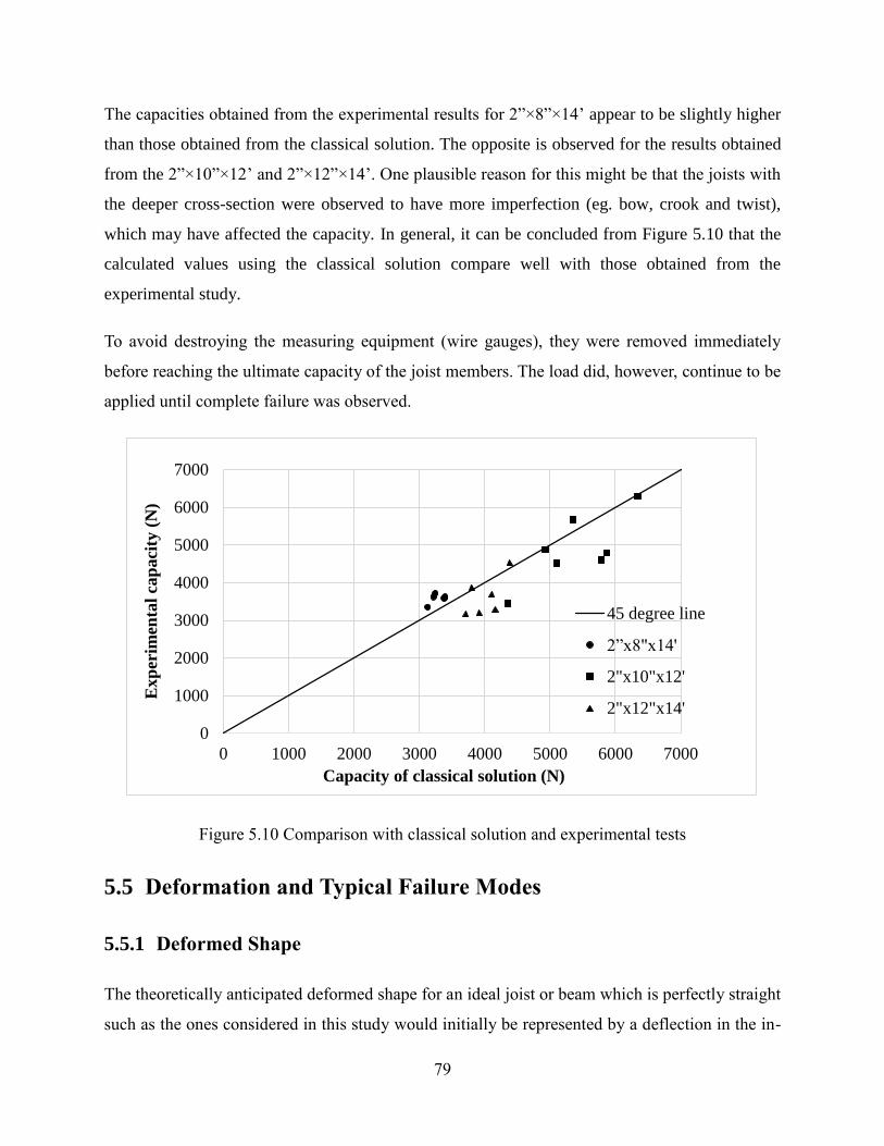
79
The capacities obtained from the experimental results for 2”×8”×14’ appear to be slightly higher
than those obtained from the classical solution. The opposite is observed for the results obtained
from the 2”×10”×12’ and 2”×12”×14’. One plausible reason for this might be that the joists with
the deeper cross-section were observed to have more imperfection (eg. bow, crook and twist),
which may have affected the capacity. In general, it can be concluded from Figure 5.10 that the
calculated values using the classical solution compare well with those obtained from the
experimental study.
To avoid destroying the measuring equipment (wire gauges), they were removed immediately
before reaching the ultimate capacity of the joist members. The load did, however, continue to be
applied until complete failure was observed.
Figure 5.10 Comparison with classical solution and experimental tests
5.5 Deformation and Typical Failure Modes
5.5.1 Deformed Shape
The theoretically anticipated deformed shape for an ideal joist or beam which is perfectly straight
such as the ones considered in this study would initially be represented by a deflection in the in-
0
1000
2000
3000
4000
5000
6000
7000
0 1000 2000 3000 4000 5000 6000 7000
Exp
erim
enta
l ca
paci
ty (
N)
Capacity of classical solution (N)
45 degree line
2”x8"x14'
2"x10"x12'
2"x12"x14'

80
plane direction, until reaching a critical moment, after which the bending member would start to
deform laterally (Galambos & Surovek, 2008). However, due to initial imperfection in the real
wood member (e.g. crook and bow), the joist was observed to deflect in the out-of-plane direction
before the critical moment was reached. This is illustrated schematically in Figure 5.11, and was
also observed in the experimental results as shown in Figures 5.7, 5.8 and 5.9. Therefore, in
addition to the geometry and mechanical properties, the critical load and failure of the real beam
is also influenced by the imperfection and non-linear deformation (Ahnlén, 2013).
Figure 5.11 The lateral deflection of ideal beam and real beam
Figure 5.12 shows a typical deformed shape during a full scale lateral torsional buckling test. As
it can be seen in Figures 5.12 (b) and (c), there is significant out-of-plane deformation and twist in
the beam, which decreased gradually towards the end supports.

81
(a)
(b)
(c)
Figure 5.12 Typical LTB deformation in the test
(a) initial stage of LTB test, (b) final stage of LTB test, and (c) typical top view of LTB
deformation in the test
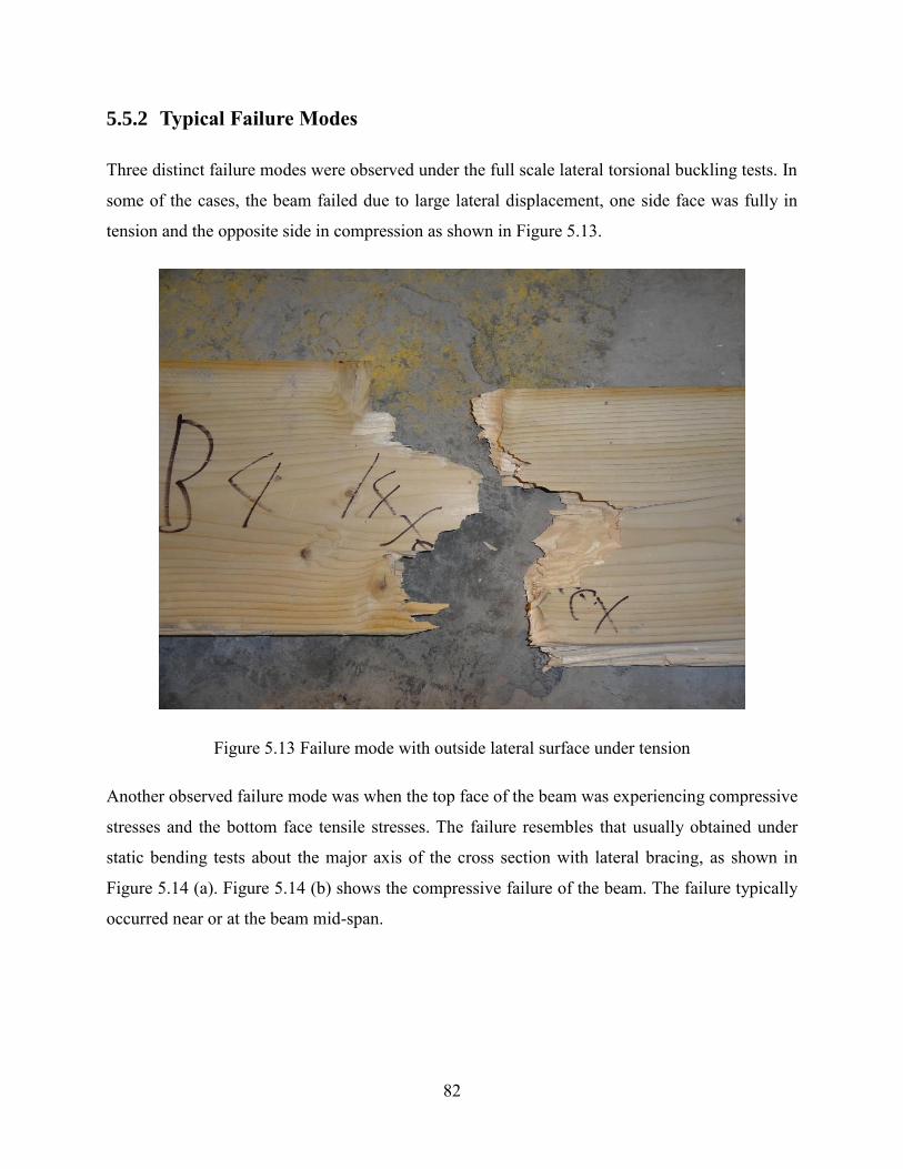
82
5.5.2 Typical Failure Modes
Three distinct failure modes were observed under the full scale lateral torsional buckling tests. In
some of the cases, the beam failed due to large lateral displacement, one side face was fully in
tension and the opposite side in compression as shown in Figure 5.13.
Figure 5.13 Failure mode with outside lateral surface under tension
Another observed failure mode was when the top face of the beam was experiencing compressive
stresses and the bottom face tensile stresses. The failure resembles that usually obtained under
static bending tests about the major axis of the cross section with lateral bracing, as shown in
Figure 5.14 (a). Figure 5.14 (b) shows the compressive failure of the beam. The failure typically
occurred near or at the beam mid-span.

83
(a)
(b)
Figure 5.14 Failure mode with top face under compression and bottom face under tension
(a) Profile, and (b) top view
The third observed failure mode is longitudinal shear as shown in Figure 5.15. The torsional shear
crack was usually located around the mid-height of the beam and extend along the longitudinal
direction from middle span to the end of beam.
Middle span

84
Figure 5.15 Failure mode by shear stress
5.6 Notation for Chapter 5
b beam width (mm)
d beam depth (mm)
LE modulus of elasticity along the longitudinal direction (MPa)
TG shear modulus about transverse (MPa)
J Saint Venant Torsional constant (mm4)
k constant depending on the aspect ratio /d b
iL distance between inclinometers (mm)
T applied torque force (Nmm)
angle of twist (degree)

85
5.7 References
[1] ASTM Standard D198. (2009). Standard Test Method of Static Tests of Lumber in Structural
Sizes. Philadelphia, Pa.
[2] Hibbeler R.C., (2011). Mechnics of Materials, Eighth Edition, Pearson Prentice Hall, USA.
[3] Yang, Z. (2012). Torsional Shear Strength and Size Effect in Structural Composite Lumber.
M.A.Sc Thesis, Department of Environmental Conservation, University of Massachusetts
Amherst, Amherst, Massachusetts. USA.
[4] Khokhar, A., and Zhang, H. (2012). The use of torsion test method to evaluate the shear
properties of timber joists. In World Conference on Timber Engineering, Auckland.
[5] Galambos T. V. and Surovek. A. E. (2008). Structural Stability of Steel: Concepts and
Applications for Structural Engineers, John Wiley & Sons, Inc. Hoboken, New Jersey. USA.
[6] Ahnlén, M and Westlund, J. (2013). Lateral Torsional Buckling of I-beams. M.A.Sc Thesis,
Department of Civil and Environmental Engineering, Chalmers University of Technology,
Göteborg, Sweden.
86
Chapter 6
Comparison between FEA Model and
Experimental Results
6.1 Model Description
6.1.1 Introduction
The objective of this chapter is to compare the FEA model with the results obtained from the
experiment. As discussed in Experimental study (Chapter 4) and in Experimental results (Chapter
5), the modulus of elasticity in the longitudinal direction ( )LE and shear modulus about the
transverse direction ( )TG were obtained from the experiments. Based on the mechanical
properties and dimensions of each specimen, finite element models were developed to investigate
the lateral torsional buckling capacity. A comparison was made between experimental programs
and numerical analyses to verify the accuracy of linear elastic Eigen value finite element analysis.
6.1.2 Mesh Details
Similar to sensitivity analysis in Chapter 3, the C3D8 eight-noded brick element beams from the
ABAQUS library of elements was used to model the entire beam (Simulia, 2011). The models
have the same dimensions as those of the experimental program. The nominal dimensions of the
specimens were 2”×8”×14’ (38mm×184mm×4267mm), 2”×10”×12’ (38mm×235mm×3658mm),
and 2”×12”×14’ (38mm×286mm×4267mm). However, as discussed in the experimental study
section (Chapter 4), the actual dimensions varied slightly from the nominal dimensions. In order
to predict the accurate capacity of each specimen, the models were developed based on the actual
sizes. In all cases, the clear spans were 4200 mm and 3600 mm . The dimensions of each model
are shown in column 1, 2, 3 and 4 of Table 6.1.

87
In order to unify the mesh, all beams in the same nominal size were modelled with identical mesh,
i.e., the number of elements along the width, height and length were kept constant for 2”x8”x14’,
2”×10”×12’ and 2”×12”×14’ specimens. Similar to the sensitivity analysis, to ensure the best
results, the value of width and height for each element were chosen to be close while the length of
the element was taken as approximately twice the width. The mesh is fully defined by four
parameters1m , 2m ,
3m and 4m as shown in Figure 6.1. Typical element dimensions were nearly
3.8 mm in width and height and about 7.6 mm in length. The mesh parameters for each specimen
modelled are presented in Column 5, 6, 7 and 8 Table 6.1.
(a)
(b)
Figure 6.1 Parameters defining the FEA mesh
(a) front view, (b) top view
Note: 1m is the number of elements along the clear span, 2m is the number of elements along the
extra part of clear span

88
6.1.3 Mechanical Properties of Material
The objective of the FEA models is to compare the critical load of experimental results with the
finite element analyses results. Each numerical model was defined with mechanical properties
identical to those of the corresponding experimental specimen. As proved in the sensitivity analysis
(Chapter 3), only the modulus of elasticity in the longitudinal direction ( )LE and the shear
modulus about the transverse direction ( )TG affect the lateral torsional buckling capacity of a
beam. The values of LE and TG have been obtained through testing in experiments and the results
have been provided in the experimental results section (Chapter 5). The rest of the mechanical
properties for all the models are consistent with the model in the sensitivity analysis. The values
of these parameters are provided in table 6.1.
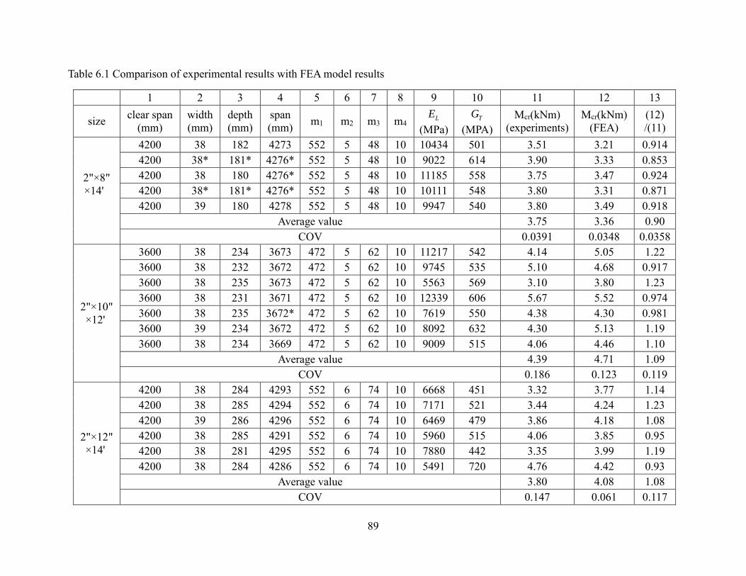
89
Table 6.1 Comparison of experimental results with FEA model results
1 2 3 4 5 6 7 8 9 10 11 12 13
size clear span
(mm)
width
(mm)
depth
(mm)
span
(mm) m1 m2 m3 m4
LE
(MPa)
TG
(MPA)
Mcr(kNm)
(experiments)
Mcr(kNm)
(FEA)
(12)
/(11)
2"×8"
×14'
4200 38 182 4273 552 5 48 10 10434 501 3.51 3.21 0.914
4200 38* 181* 4276* 552 5 48 10 9022 614 3.90 3.33 0.853
4200 38 180 4276* 552 5 48 10 11185 558 3.75 3.47 0.924
4200 38* 181* 4276* 552 5 48 10 10111 548 3.80 3.31 0.871
4200 39 180 4278 552 5 48 10 9947 540 3.80 3.49 0.918
Average value 3.75 3.36 0.90
COV 0.0391 0.0348 0.0358
2"×10"
×12'
3600 38 234 3673 472 5 62 10 11217 542 4.14 5.05 1.22
3600 38 232 3672 472 5 62 10 9745 535 5.10 4.68 0.917
3600 38 235 3673 472 5 62 10 5563 569 3.10 3.80 1.23
3600 38 231 3671 472 5 62 10 12339 606 5.67 5.52 0.974
3600 38 235 3672* 472 5 62 10 7619 550 4.38 4.30 0.981
3600 39 234 3672 472 5 62 10 8092 632 4.30 5.13 1.19
3600 38 234 3669 472 5 62 10 9009 515 4.06 4.46 1.10
Average value 4.39 4.71 1.09
COV 0.186 0.123 0.119
2"×12"
×14'
4200 38 284 4293 552 6 74 10 6668 451 3.32 3.77 1.14
4200 38 285 4294 552 6 74 10 7171 521 3.44 4.24 1.23
4200 39 286 4296 552 6 74 10 6469 479 3.86 4.18 1.08
4200 38 285 4291 552 6 74 10 5960 515 4.06 3.85 0.95
4200 38 281 4295 552 6 74 10 7880 442 3.35 3.99 1.19
4200 38 284 4286 552 6 74 10 5491 720 4.76 4.42 0.93
Average value 3.80 4.08 1.08
COV 0.147 0.061 0.117
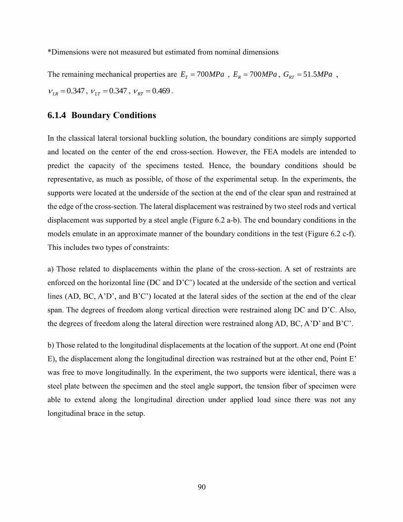
90
*Dimensions were not measured but estimated from nominal dimensions
The remaining mechanical properties are 700TE MPa , 700RE MPa , 51.5RTG MPa ,
0.347LR , 0.347LT , 0.469RT .
6.1.4 Boundary Conditions
In the classical lateral torsional buckling solution, the boundary conditions are simply supported
and located on the center of the end cross-section. However, the FEA models are intended to
predict the capacity of the specimens tested. Hence, the boundary conditions should be
representative, as much as possible, of those of the experimental setup. In the experiments, the
supports were located at the underside of the section at the end of the clear span and restrained at
the edge of the cross-section. The lateral displacement was restrained by two steel rods and vertical
displacement was supported by a steel angle (Figure 6.2 a-b). The end boundary conditions in the
models emulate in an approximate manner of the boundary conditions in the test (Figure 6.2 c-f).
This includes two types of constraints:
a) Those related to displacements within the plane of the cross-section. A set of restraints are
enforced on the horizontal line (DC and D’C’) located at the underside of the section and vertical
lines (AD, BC, A’D’, and B’C’) located at the lateral sides of the section at the end of the clear
span. The degrees of freedom along vertical direction were restrained along DC and D’C. Also,
the degrees of freedom along the lateral direction were restrained along AD, BC, A’D’ and B’C’.
b) Those related to the longitudinal displacements at the location of the support. At one end (Point
E), the displacement along the longitudinal direction was restrained but at the other end, Point E’
was free to move longitudinally. In the experiment, the two supports were identical, there was a
steel plate between the specimen and the steel angle support, the tension fiber of specimen were
able to extend along the longitudinal direction under applied load since there was not any
longitudinal brace in the setup.

91
(a)
(b)
(c)
(d)
(e)
(f)
Figure 6.2 Boundary conditions (crossed arrows denote restrained DOFs)
(a) Experimental End Detail, (b) Elevation of Experimental end detail, (c) DOFs Restrained at
left end, (d) DOFs Restrained at right end, (e) Left end in ABAQUS model, and (f) Right end in
ABAQUS model

92
6.1.5 Modelling of Load Application
In the experiments, the beams were subjected to a mid-span load applied at the top face of the
beam (Figures 6.3 a, b). The load was applied on the small area and remained vertical when the
beam buckled laterally. In order to avoid stress concentration at the load point and try to model the
load as close as possible to the setup, the concentrated load was constituted of forty-nine
concentrated loads on forty-nine nodes which are on a small area at the center of the clear span,
and the magnitude of the individual concentrated load decreased progressively from the center to
the edge of the small area, as shown in Figure 6.3 c and d.
(a)
(b)
(c)
(d)
Figure 6.3 Load Application Detail
(b) Experimental Details and (c) and (d) Corresponding FEA model Detail

93
6.2 Results of FEA model and comparison
By running each FEA model with linear Eigen-value analysis and obtaining the critical load which
is applied at the center of the beams, a comparison was established between experimental programs
and the numerical analysis. As shown in column 11 and 12 of Table 6.1 and Figure 6.4. It can be
seen that the results of the numerical model are close to the experimental results. The obtained
results from FEA model and experimental work are found in the vicinity of MFEA=Mtest line and
the average ratio of the models with experiments is 1.03 and coefficient of variation (COV) of all
ratios is 0.132, the average ratio of 2”×8”×14’, 2”×10”×12’ and 2”×12”×14’ beams are 0.9, 1.09
and 1.08 respectively. A large portion of ratios are within the range of 0.9 to 1.1, the lowest value
observed is 0.853 and the highest value is found to be 1.23. The COV of ratios are 0.0358, 0.119
and 0.117 for the three standard sizes beam respectively, since the 2”×8”×14’ specimens have
better conditions (less defects and imperfections) and stable values of modulus of elasticity and
shear modulus due to the smaller dimensions than 2”×10”×12’ and 2”×12”×14’ beams. The COV
of ratios of standard size 2”×8”×14’ is much smaller than the other dimensions specimens. In
Hooley and Madsen’s lateral torsional buckling test of glue-laminated timbers, the ratio of critical
stress of the test with critical stress of lateral torsional buckling theory falls under the limits of 0.81
to 1.19, and the average value of ratios and COV of ratios are 0.994 and 0.104 respectively (Hooley
and Madsen, 1964). The variation range of ratios are similar as that shown in Table 6.1, however,
the COV of all ratios shown in Table 6.1 is higher than Hooley and Madsen’s tests, one possible
reason is glue-laminated timber has less imperfections to affect critical moment except mechanical
properties than sawn lumber. In general, the values shown in Table 6.1 are found to be similar to
the of the results of Hooley and Madsen’s test. Based on the results and comparison, the models
are able to capture the beams behaviour. Figure 6.4 provides the plot of experimental and FEA
model results. The typical buckling shape of experiments and FEA model of each standard size
subjected to concentrated load at the center are shown in Figure 6.5, 6.6 and 6.7.

94
Figure 6.4 Comparison of experiemtnal results and FEA model results
0
1
2
3
4
5
6
0 1 2 3 4 5 6
Cri
tica
l m
om
ent
of
FE
mod
els
(kN
m)
Critical moment of experiments (kNm)
2"x8"x12'
2"x10"x12'
2"x12"x14'
Mcr(FEA)=Mcr(Experiments)
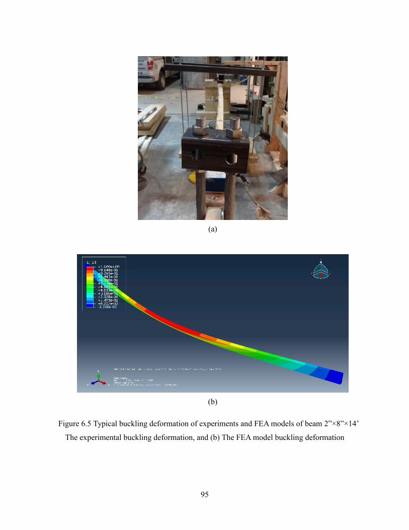
95
(a)
(b)
Figure 6.5 Typical buckling deformation of experiments and FEA models of beam 2”×8”×14’
The experimental buckling deformation, and (b) The FEA model buckling deformation

96
(a)
(b)
Figure 6.6 Typical buckling deformation of experiments and FEA models of beam 2”×10”×12’
(a) The experimental buckling deformation, and (b) The FEA buckling deformation

97
(a)
(b)
Figure 6.7 Typical buckling deformation of experiments and FEA models of beam 2”×12”×14’
(a) The experimental buckling deformation, and (b) The FEA buckling deformation
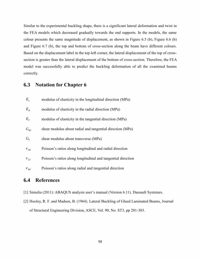
98
Similar to the experimental buckling shape, there is a significant lateral deformation and twist in
the FEA models which decreased gradually towards the end supports. In the models, the same
colour presents the same magnitude of displacement, as shown in Figure 6.5 (b), Figure 6.6 (b)
and Figure 6.7 (b), the top and bottom of cross-section along the beam have different colours.
Based on the displacement label in the top-left corner, the lateral displacement of the top of cross-
section is greater than the lateral displacement of the bottom of cross-section. Therefore, the FEA
model was successfully able to predict the buckling deformation of all the examined beams
correctly.
6.3 Notation for Chapter 6
LE modulus of elasticity in the longitudinal direction (MPa)
RE modulus of elasticity in the radial direction (MPa)
TE modulus of elasticity in the tangential direction (MPa)
RTG shear modulus about radial and tangential direction (MPa)
TG shear modulus about transverse (MPa)
LR Poisson’s ratios along longitudinal and radial direction
LT Poisson’s ratios along longitudinal and tangential direction
RT Poisson’s ratios along radial and tangential direction
6.4 References
[1] Simulia (2011): ABAQUS analysis user’s manual (Version 6.11). Dassault Systemes.
[2] Hooley, R. F. and Madsen, B. (1964). Lateral Buckling of Glued Laminated Beams, Journal
of Structural Engineering Division, ASCE, Vol. 90, No. ST3, pp 201-303.

99
Chapter 7
Parametric Study
7.1 Scope
The comparisons between the finite element and experimental results in Chapter 6 have validated
the finite element model. The validated FEA model is used in the present chapter to conduct a
parametric study aimed at investigating four effects on the lateral torsional buckling capacity: a)
the load height effect, b) the location of end support restraint along the height of the cross-section,
c) the effect of beam dimensions and d) the effect of warping contribution in buckling capacity.
7.2 Mesh Details
Similar to the sensitivity analysis in Chapter 3 and FEA model in Chapter 6, the C3D8 eight-noded
brick element was used to model the problem. The dimensions of models are 2”×12”×12’,
2”×12”×10’, 2”×12”×14’ and 2”×10”×12’. The mesh is fully defined by the numbers of elements
1n along height, the number of elements 2n along the width, and the number of elements 3n along
the span (Figure 7.1). The number of elements 1n is 76 for the 286 mm deep beams and 62 for 235
mm deep beams. Parameter 2n take the value 10 in all runs, while parameter 3n takes the values
562, 482, and 402 for the 4267 mm, 3658 mm, and 3048 mm span beams, respectively.

100
Figure 7.1 Finite Element Mesh
7.3 Mechanical properties
The finite element model was developed for Spruce-pine-fir NO.1/NO.2 grade of wood. The mean
value of modulus of elasticity in the longitudinal direction ( LE ) reported in (CAN/CSA O86-09,
2009) was chosen as a reference value. Since Spruce-Pine-Fir (SPF) represents a group of wood
species with similar characteristics, the properties of Lodgepole Pine (a species of SPF) were
chosen to develop the model. CAN/CSA O86-09 does not provide the values of shear modulus and
Poisson’s ratio. Therefore, the mechanical properties (Modulus of elasticity about radial RE and
tangential direction TE , Shear modulus about longitudinal and radial direction LRG and about
longitudinal and tangential direction LTG and about radial and tangential direction RTG , Poisson’s
ratios along longitudinal and radial direction LRv , and along longitudinal and radial direction LTv ,
and along radial and tangential direction RTv ) were taken based on the ratio of LE as reported in
Wood handbook (FPL, 2010).
Since the difference between the properties in the radial and tangential direction (modulus of
elasticity in radial direction RE and tangential direction TE ) can be considered insignificant
(Isopescu, 2012), it can be assumed that they are equal, i.e., R T tE E E , where the parameters
about the transverse direction should be obtained from experiments. Also, the shear modulus LRG

101
and LTG can be assumed equal, i.e., LR LT TG G G and Poisson’s ratios
LR LT T . Thus,
in the FEA model, the values of the mechanical parameters taken are shown in Table 7.1
Table 7.1 The mechanical parameters of Spruce-Pine-Fir
Parameter Value
LE 9500 MPa
tE 808 MPa
TG 451 MPa
RTG 47.5 MPa
T 0.332
RT 0.469
7.4 Analyses to Investigate Effect of Load Position
In the classical lateral torsional buckling solution, the critical moment is equal to the result of the
classical solution multiplied by the load eccentricity factor, as shown in Equation 7.1. When the
bending moment is applied on the neutral axis, the load eccentricity factor 1.0eC .
cr e b uM C C M (7.1)
where
2
Lu L T y w
u u
y
EM E I G J I C
L L
(7.2)
in which bC is equivalent moment factor which accounts for the moment gradient (Equation 2.6
in Chapter 2), eC is the load eccentricity factor which accounts for the load position effect. It is
provided in (AFPA, 2003) as
2 1eC (7.3)

102
where
2
L y
u T
E IKd
L G J (7.4)
in which d is the depth of the cross-section. Negative values of η mean that the load is applied
below the centroid and positive values denote loads applied above the centroid (AFPA, 2003).
Symbol Lu is the unbraced span of the beam. Constant K takes the value 1.72K when the beam
is under concentrated load at center of length and the value 1.44K when the beam is under
uniformly distributed load.
7.4.1 Background
The classical lateral torsional buckling solution (Equation 7.2) is based on loads which are applied
at the centroid of the rectangular section. However, in practical situations, the load is located on
the top face of the beam. In such a case, as discussed in the literature review section, an additional
destabilizing twisting moment is induced by the vertical load undergoing a horizontal displacement
relative to the section centroid. Conversely, when the load acts on the bottom of the beam, the
resulting twisting moments have a stabilizing effect and increase the capacity of the member. Thus
section conducts a buckling FEA in which all three loading positions are investigated. A
comparison is then made with results based on the load eccentricity factor eC as determined from
Equation (7.3).
7.4.2 Boundary condition and load patterns
The reference model is a simply supported beam, similar to that adopted in the sensitivity analysis.
The boundary supports are located on the mid-height of the end cross-section, in a manner similar
to the classical solution. The end cross-section was free to rotate about the major and minor axes.
In the longitudinal direction, the left end was restrained and the other end was free to move.
Two loading patterns are investigated by the model. The first loading pattern was a concentrated
load at the beam mid-span and the second one was a uniformly distributed load. For each loading
pattern, three cases were considered concerning to the location of the load relative to the section

103
centroid. (a) top face loading, (b) centroidal loading, and (c) bottom face loading. For the case of
centroidal loading, half of the load was applied to the top face and the other half on the bottom
face (Figs. 7.2 a-f)
(a)
(b)
(c)
(d)
(e)
(f)
Figure 7.2 Simply supported beam under concentrated load at mid-span and uniformly
distributed load acting at (a) (b) top face, (c) (d) centroid, and (e) (f) bottom face.
Similar to the FEA models in Chapter 6, the concentrated load was applied as a series of forty-nine
concentrated loads acting on a small area (45.5mm×22.8mm) at the center of span. For the
uniformly distributed load, a series of concentrated loads were applied to the middle line of the top
and bottom faces (Figure 7.3).

104
Figure 7.3 The constitution of uniformly distributed load
7.4.3 Load eccentricity factor
For the dimensions of the cross-section of the reference model (38mm on width and 286mm on
depth), the values of the eccentricity factor as determined from Equation (7.3) for different load
options and locations are shown in column 13 of Table 7.2 and 7.3.
7.4.4 Observations and results
The critical moments of the FEA model under a concentrated load at the center are presented for
the reference beam and beam number A1 and A2 in ninth column of Table 7.2. When the load was
applied on the top face (A1), the critical moment decreased, and conversely, when the load was
applied on the bottom face (A2), the critical moment increased. In order to compare the eccentricity
factors of FEA model with Equation (7.3) and (7.4), a comparison is made between the FEA
models and the classical solution (Column 10-13) which includes the equivalent moment factor,
load eccentricity factor and critical moment. Based on the ratio between the results of the FEA
models and classical solution which is presented in the column 14, the difference of the two
methods is insignificant. Therefore, it can be seen that the model is able to capture the eccentricity
factors provided in (AFPA, 2003)
Table 7.3 shows the same comparison as Table 7.2, for the FEA models under uniformly distributed
load. The same results of Table 7.2 are observed in Table 7.3.
105
7.5 Analyses to Investigate Effect of Support Height
7.5.1 Motivation
The classical lateral torsional buckling solution is based on supports which are located at the
centroid of the end cross-section. However, practically in connection design and construction, the
point of restraint may be located above or below than the section centroid. Also, in the tests
performed in Chapter 4 and 5, the points of support were located at the bottom face. It is thus of
practical interest to investigate the effect of the support location relative to the section centroid.
7.5.2 Loading Patterns and Boundary Condition Details
Two loading cases were considered: a mid-span load and a uniformly distributed load. For each
loading, three load positions were considered: top face loading, centroid loading and bottom face
loading.
Figure 7.4 (a) shows the reference case where the supports are located at mid-height of the beam,
this case is analogous to the classical solution which has been performed in Chapter 3. In Figure
7.4 (b), the supports are located at the bottom, the beam is simply supported and free to rotate
about weak and strong axis. The boundary conditions are illustrated in Figure 7.5a-d and include
two types of constraints:
a) Those related to displacements within the plane of the cross-section where a set of restraints are
enforced on the horizontal lines (AB and A’B’) located at the underside of the section and vertical
lines (CD and C’D’). Degrees of freedom along vertical direction were restrained at AB and A’B’.
Degrees of freedom along lateral direction were restrained at CD and C’D’.
b) Those related to longitudinal displacements at the location of the support. At one end (Point C),
the displacement along the longitudinal direction was restrained but at the other end, Point C’ was
free to move longitudinally.

106
(a)
(b)
Figure 7.4 The location of supports at (a) Mid-height of beam, and (b) bottom of beam.

107
(a)
(b)
(c)
(d)
Figure 7.5 The boundary condition located on the bottom (a) restriction of left end cross-section,
(b) restriction of right end cross-section, (c) Left end in ABAQUS model, and (d) right end in
ABAQUS model

108
7.5.3 Observations and Results
Beam number A3, A4, A5 in Table 7.2 present the details and results of boundary conditions
located at the bottom of beam under concentrated load at mid-span. The lateral torsional buckling
capacity of FEA model are shown in column 9. Comparing with the critical moment of column 9
of A0, A1 and A2 (supports located at mid-height), there are no significant changes after moving
the supports from middle height to bottom (A0=A3, A1=A4 and A2=A5). Also, the same
comparisons are made for the uniformly distributed load (Table 7.3), similar as Table 7.2, the effect
of moving the support from mid-height to bottom can be neglected.
7.6 Effect of Dimension
7.6.1 Dimensions
According to the classical lateral torsional buckling solution, the capacity of a beam is not only
affected by mechanical properties but also the dimensions of the beam, three models were
developed based on changing one dimension of the reference model and then compared the results
with the reference case. The first two were varying the length of the reference model from 12 feet
(3658mm) to 14 feet (4267mm) and 10 feet (3048mm) while keeping the dimension of cross-
section unchanged, the last one was changing the depth of reference model from 12 inch (286mm)
to 10 inch (235mm) while keeping the width 2 inch (38mm) and length 12 feet (3658mm)
unchanged. The mechanical properties were taken identical to those of the reference model (Table
7.1).
7.6.2 Boundary Condition and Load Patterns
The beam is simply supported and under concentrated load at center of span and uniformly
distributed load, the end cross-sections were free to rotate about weak and strong axis and the
restrictions were located on the center of the end cross-section.
7.6.3 Observation and Results
A6, A7 and A8 in Column 9 of Table 7.2 presented the details and results models with different

109
dimensions. The results of A6, and A7 in column 10 show that with the same dimension of cross-
section, an inverse relationship occurred between lateral torsional buckling resistance and beam
span, the lateral torsional buckling resistance increased with the reduction of span, just the opposite,
the resistance decreased with the increase of length. The column 13 (classical solution) of Table
7.2 present the same trend. The same observations are also observed in uniformly distributed load
of B6 and B7.
The result of A8 in column 9 of Table 7.2 shows that the identical relationship happened between
lateral torsional buckling resistance and depth, the lateral torsional buckling resistance decreased
with the reduction of depth. Comparing with classical solution (Column 13), all the observations
between buckling resistance and dimensions from FEA model present the same trend of classical
solution. The same observations are also observed in the uniformly distributed load of B8.
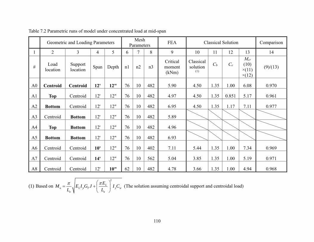
110
Table 7.2 Parametric runs of model under concentrated load at mid-span
Geometric and Loading Parameters Mesh
Parameters FEA Classical Solution Comparison
1 2 3 4 5 6 7 8 9 10 11 12 13 14
# Load
location
Support
location Span Depth n1 n2 n3
Critical
moment
(kNm)
Classical
solution (1)
Cb
Ce
Mcr
(10)
×(11)
×(12)
(9)/(13)
A0 Centroid Centroid 12' 12" 76 10 482 5.90 4.50 1.35 1.00 6.08 0.970
A1 Top Centroid 12' 12" 76 10 482 4.97 4.50 1.35 0.851 5.17 0.961
A2 Bottom Centroid 12' 12" 76 10 482 6.95 4.50 1.35 1.17 7.11 0.977
A3 Centroid Bottom 12' 12" 76 10 482 5.89
A4 Top Bottom 12' 12" 76 10 482 4.96
A5 Bottom Bottom 12' 12" 76 10 482 6.93
A6 Centroid Centroid 10' 12" 76 10 402 7.11 5.44 1.35 1.00 7.34 0.969
A7 Centroid Centroid 14' 12" 76 10 562 5.04 3.85 1.35 1.00 5.19 0.971
A8 Centroid Centroid 12' 10" 62 10 482 4.78 3.66 1.35 1.00 4.94 0.968
(1) Based on
2
Lu L T y w
u u
y
EM E I G J I C
L L
(The solution assuming centroidal support and centroidal load)
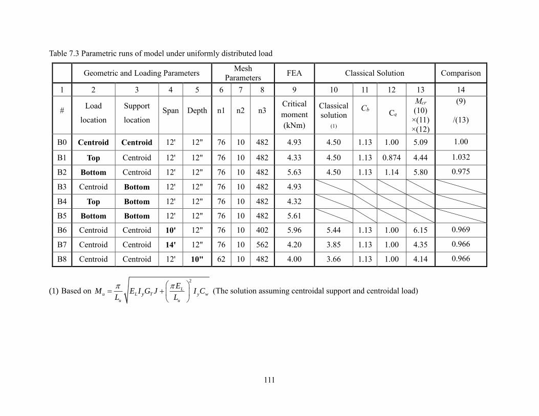
111
Table 7.3 Parametric runs of model under uniformly distributed load
Geometric and Loading Parameters Mesh
Parameters FEA Classical Solution Comparison
1 2 3 4 5 6 7 8 9 10 11 12 13 14
# Load
location
Support
location
Span Depth n1 n2 n3 Critical
moment
(kNm)
Classical
solution
(1)
Cb
Ce
Mcr
(10)
×(11)
×(12)
(9)
/(13)
B0 Centroid Centroid 12' 12" 76 10 482 4.93 4.50 1.13 1.00 5.09 1.00
B1 Top Centroid 12' 12" 76 10 482 4.33 4.50 1.13 0.874 4.44 1.032
B2 Bottom Centroid 12' 12" 76 10 482 5.63 4.50 1.13 1.14 5.80 0.975
B3 Centroid Bottom 12' 12" 76 10 482 4.93
B4 Top Bottom 12' 12" 76 10 482 4.32
B5 Bottom Bottom 12' 12" 76 10 482 5.61
B6 Centroid Centroid 10' 12" 76 10 402 5.96 5.44 1.13 1.00 6.15 0.969
B7 Centroid Centroid 14' 12" 76 10 562 4.20 3.85 1.13 1.00 4.35 0.966
B8 Centroid Centroid 12' 10" 62 10 482 4.00 3.66 1.13 1.00 4.14 0.966
(1) Based on
2
Lu L T y w
u u
y
EM E I G J I C
L L
(The solution assuming centroidal support and centroidal load)

112
7.7 Effect of Warping Contribution in Buckling Capacity
7.7.1 Motivation
In classical lateral torsional buckling solution, the resistance provided by warping is
considered. In order to explore the contribution of warping in buckling capacity of
rectangular cross-section, a comparison was made with FEA model, classical solution
with and without the resistance provided by warping to investigate the effect of warping.
7.7.2 Boundary Conditions, Load Pattern and Dimension
Since the classical lateral torsional buckling solution is based on loads and boundary
conditions which are located at the centroid, the reference cases which is simply
supported beam under uniformly distributed load and concentrated load at mid-span
were used to investigate the effect of warping in the buckling resistance. The
dimensions of reference model are 2”×12”×12’ (38mm×286mm×3658mm).
7.7.3 Observation and Results
The mechanical properties have been provided in Table 7.1, substituted the parameters
into Equation (7.5) and (7.6), the buckling capacities are 4.50 kNm and 4.44 kNm.
Since the reference cases are under uniformly distributed load and concentrated load,
the results of Equation (7.5) and (7.6) should multiply the equivalent moment factor
bC . The comparison with classical solution and FEA reference models are shown in
Table 7.4
2
Lu L T y w
u u
y
EM E I G J I C
L L
(7.5)
u L T
u
yM E I G JL
(7.6)

113
Table 7.4 Comparison with FEA model, classical solution with and without warping
constant
1 2 3 4
Load patterns Cb
Classical solution
with warping
constant (kNm)
(Equation 7.5)
Classical solution
without warping
constant (kNm)
(Equation 7.6)
FEA
model
(kNm)
Uniformly
distributed load 1.35 6.08 5.99 5.90
Concentrated
load 1.13 5.09 5.02 4.93
As shown in Table 7.4, the buckling capacity of the FEA model, classical solution with
and without warping constant are similar, the differences are insignificant. Therefore,
the warping contribution is negligible for rectangular section in buckling capacity.
7.8 Summary
The finite element model developed in this chapter accounts for the effect of a) load
positions (top face, centroid, and bottom face), b) support locations (centroid and
bottom), c) dimensions (length and depth), d) warping contribution of buckling capacity
for rectangular section.
a) Comparing with the load applied on centroid, the load acts on the top face of beam
would decrease the buckling capacity, and in contrast, the buckling capacity would
be increased when the load acts on the bottom face. The FEA models are able to
capture the eccentricity factors provided in (AFPA, 2003)
b) Comparing with the support locates on the mid-height, the support locates on the
bottom has negligible effect of buckling capacity.
c) Comparing with the reference beam case, there is an inverse relationship between
buckling capacity with length. However, with the increase in beam depth, an
increase in the buckling capacity was observed.
d) Comparing with the reference beam case in FEA model and classical solution, the
warping contribution of buckling capacity can be neglected for a rectangular section.

114
7.9 Notation for Chapter 7
bC the equivalent moment factor
eC load eccentricity factor
wC the warping constant
d beam depth (mm)
LE modulus of elasticity along the longitudinal direction (MPa)
RE modulus of elasticity along the radial direction (MPa)
TE modulus of elasticity along the tangential direction (MPa)
tE modulus of elasticity about transverse (MPa)
LRG shear modulus about longitudinal and radial direction (MPa)
LTG shear modulus about longitudinal and tangential direction (MPa)
RTG shear modulus about radial and tangential direction (MPa)
yI moment of initial in weak axis (mm4)
J Saint Venant torsion constant (mm4)
K Constant based on loading and boundary conditions
uL the unbraced length of beam
uM the critical moment of simply supported beam under constant moment
crM critical moment of beam
LR Poisson’s ratios along longitudinal and radial direction
LT Poisson’s ratios along longitudinal and tangential direction
RT Poisson’s ratios along radial and tangential direction
T Poisson’s ratios about transverse

115
7.10 References
[1] Canadian Standards Association. (2009). CSA standards O86-09, Engineering
design in wood, Mississauga, Ontario, Canada.
[2] Forest Products Labratory. (2010). Wood Handbook-Wood as an Engineering
Material. Madison, USA.
[3] Isopescu, D., Stanila, O., and Asatanei, I. (2012). Analysis of Wood Bending
Properties on Standardized Samples and Structurals Size Beams Tests, Buletinul
Insititutului PolitehnicDIN Din Iasi, Publicat de Universitatea Tehnică „Gheorghe
Asachi” din Iaşi.
[4] American Forest and Paper Association. (2003). Technical Report 14: Deisigning
for lateral-torsional stability in wood members. Washington, D.C.

116
Chapter 8
Conclusion and Recommendation
8.1 Summary and Conclusions
Following are the conclusions obtained as the result of the current study;
1) Through the sensitivity analysis, it was shown that only the modulus of elasticity
LE along the longitudinal direction and the shear modulus TG about the transverse
direction affect the critical moment of beam. In contrast, the modulus of elasticity
about the transverse direction, tE , Poisson’s ratios T and RT and the shear
modulus RTG have negligible effect on the critical moment.
2) Through experimental testing, the critical moment of rectangular sawn lumber
beam was shown to follow the classical lateral torsional buckling solution.
3) Through detailed Buckling FEA with identical dimensions, mechanical properties,
load patterns and boundary condition to those of the experimental specimens, the
FEA models were capable to predict the critical moments comparable to those
observed in the test and the classical lateral torsional buckling solution.
4) By performing a parametric analysis using the FEA models, several observations
were made: 1) loads applied on the top face of the beam decreased the critical
moment of the beam. In contrast, loads applied on the bottom face increased its
critical moment. 2) The FEA models were shown to provide results in good
agreement with those provided by the eccentricity provided in (AFPA, 2003). 3) the
critical moment is not greatly influenced by moving the supports from mid-height
to bottom of end cross-section. 4) The critical moments decrease with the span of

117
the beam in agreement with the classical solution. However, the buckling capacity
is found to increase with section depth.
8.2 Recommendation for Future Research
1) Wood members (Sawn lumber beams) have higher degree of imperfection
compared to steel beam and members of glued-laminated timber. Other than
dimension and mechanical properties, the imperfections have an effect on the
critical moment of a beam, which the classical solution does not account for.
For future investigation, full scale testing can be performed to study the effect
of imperfections on the critical moment of the members. The developed FEA
model is able to consider the imperfections which can help verifying
experimental results with computational and analytical results.
2) The developed FEA model can also be used to investigate actual connections
used in typical beam supports.
8.3 Reference
[1] American Forest and Paper Association. (2003). Technical Report 14: Deisigning
for lateral-torsional stability in wood members. Washington, D.C.

118
Appendix A
Lateral Torsional Buckling Modes of
Experimental Testing and FEA Models
This appendix provides the buckling shape of seventeen (17) specimens obtained from
the experimental program and FEA models.
Observations
It can be seen that there is a significant out-of-plane deformation and twist in both the
experimental and FEA models beams, which decreased gradually towards the end
supports. The FEA models were able to capture the buckling shape of beams in the
experiments.

119
(a)
(b)
Figure A.1 Buckling mode of Beam 1 of 2”×8”×14’ specimens
(a) experimentally observed and (b) FEA predicted
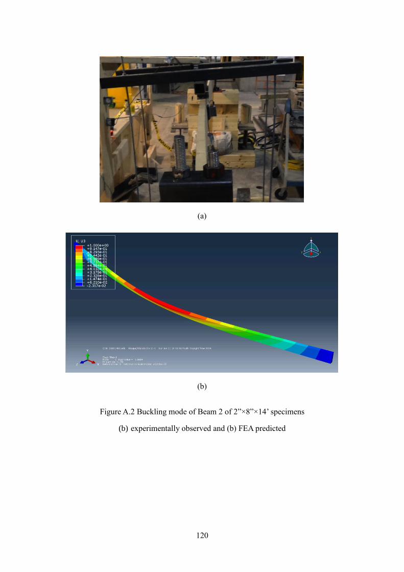
120
(a)
(b)
Figure A.2 Buckling mode of Beam 2 of 2”×8”×14’ specimens
(b) experimentally observed and (b) FEA predicted

121
(a)
(b)
Figure A.3 Buckling mode of Beam 3 of 2”×8”×14’ specimens
(c) experimentally observed and (b) FEA predicted
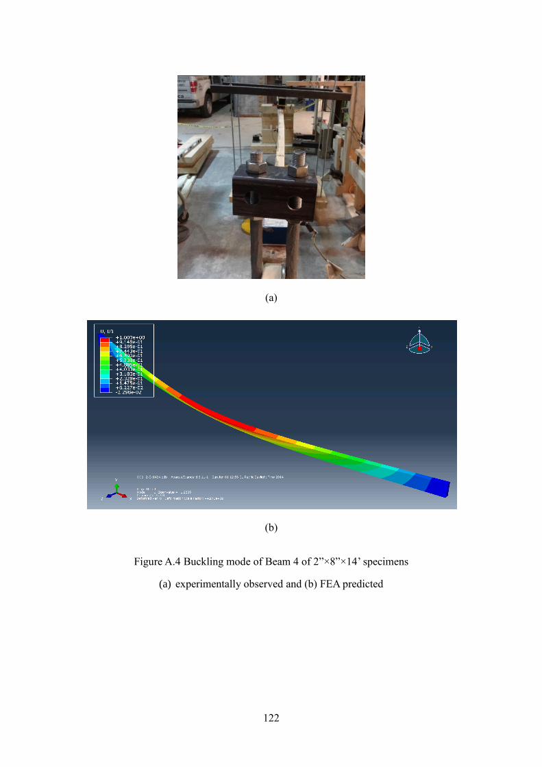
122
(a)
(b)
Figure A.4 Buckling mode of Beam 4 of 2”×8”×14’ specimens
(a) experimentally observed and (b) FEA predicted

123
(a)
(b)
Figure A.5 Buckling mode of Beam 6 of 2”×8”×14’ specimens
(a) experimentally observed and (b) FEA predicted

124
(a)
(b)
Figure A.6 Buckling mode of Beam 1 of 2”×10”×12’ specimens
(a) experimentally observed and (b) FEA predicted
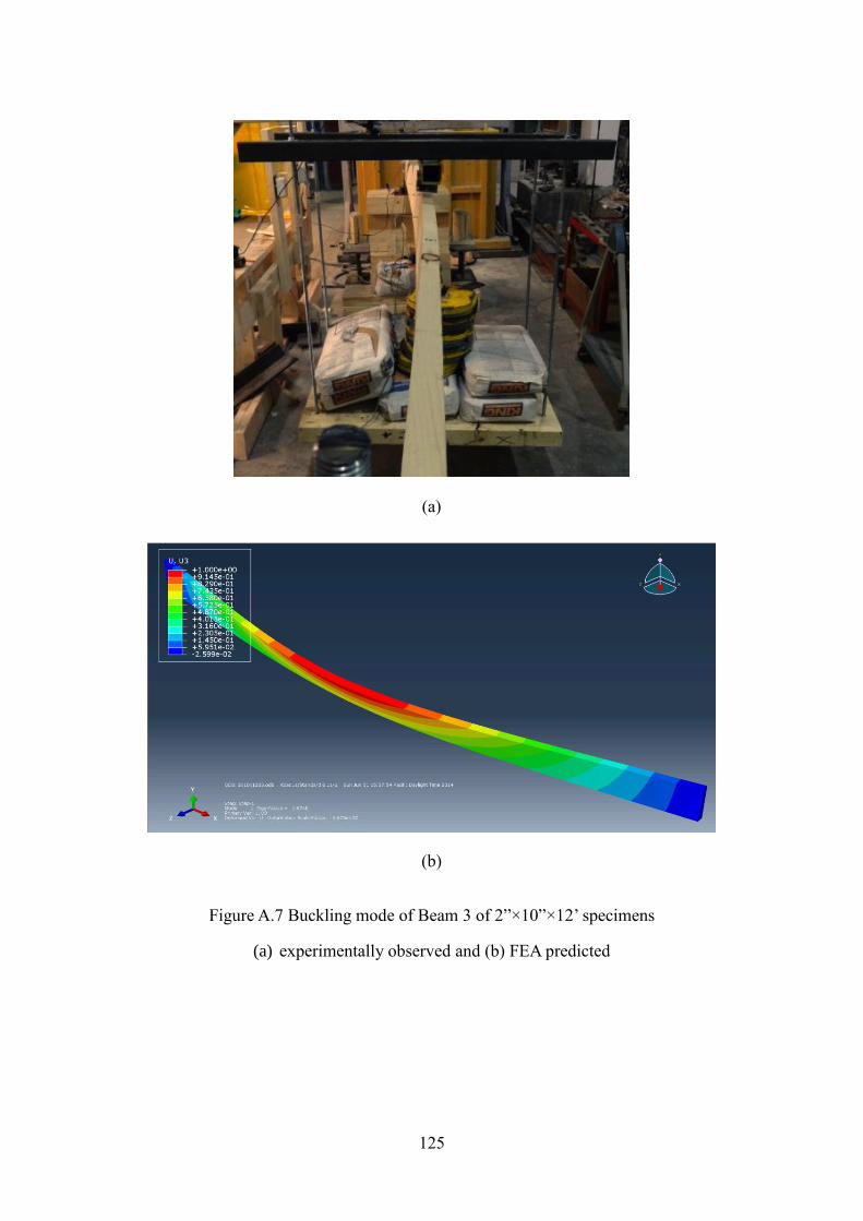
125
(a)
(b)
Figure A.7 Buckling mode of Beam 3 of 2”×10”×12’ specimens
(a) experimentally observed and (b) FEA predicted

126
(a)
(b)
Figure A.8 Buckling mode of Beam 5 of 2”×10”×12’ specimens
(a) experimentally observed and (b) FEA predicted

127
(a)
(b)
Figure A.9 Buckling mode of Beam 7 of 2”×10”×12’ specimens
(a) experimentally observed and (b) FEA predicted

128
(a)
(b)
Figure A.10 Buckling mode of Beam 2 of 2”×12”×14’ specimens
(a) experimentally observed and (b) FEA predicted

129
(a)
(b)
Figure A.11 Buckling mode of Beam 3 of 2”×12”×14’ specimens
(a) experimentally observed and (b) FEA predicted

130
(a)
(b)
Figure A.12 Buckling mode of Beam 5 of 2”×12”×14’ specimens
(a) experimentally observed and (b) FEA predicted

131
(a)
(b)
Figure A.13 Buckling mode of Beam 6 of 2”×12”×14’ specimens
(a) experimentally observed and (b) FEA predicted

132
Appendix B
Deformation of Lateral Torsional Buckling
in Experiments
This appendix provides the applied load with corresponding twist, vertical and lateral
displacement of mid-span for eleven (11) specimens form the experimental program.
The lateral displacements were the measured at mid-height and at mid-span.
Observations
The tables show a direct relation between the applied load and twist, vertical
displacement and lateral displacement of the beams.
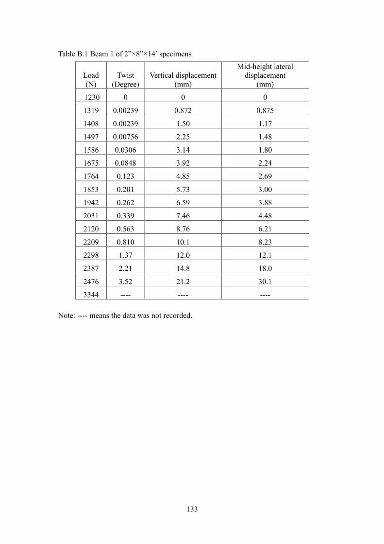
133
Table B.1 Beam 1 of 2”×8”×14’ specimens
Load
(N)
Twist
(Degree)
Vertical displacement
(mm)
Mid-height lateral
displacement
(mm)
1230 0 0 0
1319 0.00239 0.872 0.875
1408 0.00239 1.50 1.17
1497 0.00756 2.25 1.48
1586 0.0306 3.14 1.80
1675 0.0848 3.92 2.24
1764 0.123 4.85 2.69
1853 0.201 5.73 3.00
1942 0.262 6.59 3.88
2031 0.339 7.46 4.48
2120 0.563 8.76 6.21
2209 0.810 10.1 8.23
2298 1.37 12.0 12.1
2387 2.21 14.8 18.0
2476 3.52 21.2 30.1
3344 ---- ---- ----
Note: ---- means the data was not recorded.

134
Table B.2 Beam 2 of 2”×8”×14’ specimens
LOAD
(N)
Twist
(Degree)
Vertical displacement
(mm)
Mid-height lateral
displacement
(mm)
1229 0 0 0
1320 0.116 0.516 0.340
1411 0.100 1.20 0.882
1501 0.162 1.86 1.35
1592 0.185 2.52 1.98
1683 0.231 3.36 2.89
1773 0.301 4.07 3.38
1864 0.324 4.97 4.59
1955 0.301 5.82 5.86
2046 0.440 6.59 6.81
2136 0.532 7.64 8.36
2227 0.694 8.67 9.92
2318 0.887 9.81 11.9
2408 1.19 11.3 14.7
2499 2.19 13.6 20.2
2544 2.10 15.3 23.1
3719 ---- ---- ----

135
Table B.3 Beam 3 of 2”×8”×14’ specimens
LOAD
(N)
Twist
(Degree)
Vertical displacement
(mm)
Mid-height lateral
displacement
(mm)
1229 0 0 0
1320 0.031 0.712 0.233
1411 0.131 1.38 0.688
1501 0.278 2.24 1.32
1592 0.362 3.10 1.99
1683 0.447 4.01 2.60
1773 0.609 5.03 3.65
1864 0.733 5.91 4.66
1955 0.925 7.21 6.01
2046 1.15 8.34 7.59
2136 1.33 9.45 8.71
2227 1.61 10.8 10.6
2318 1.80 12.3 12.6
2408 2.11 13.9 15.0
2499 2.41 15.5 17.3
2544 2.58 16.4 18.5
2590 2.79 17.4 20.1
2635 2.99 18.7 22.3
2681 3.24 19.9 23.9
2726 3.42 21.5 26.9
2771 3.68 22.0 29.4
3576 ---- ---- ----
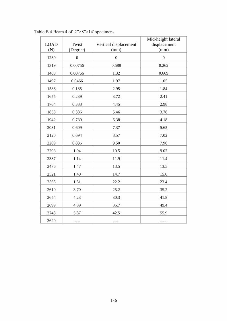
136
Table B.4 Beam 4 of 2”×8”×14’ specimens
LOAD
(N)
Twist
(Degree)
Vertical displacement
(mm)
Mid-height lateral
displacement
(mm)
1230 0 0 0
1319 0.00756 0.588 0.262
1408 0.00756 1.32 0.669
1497 0.0466 1.97 1.05
1586 0.185 2.95 1.84
1675 0.239 3.72 2.41
1764 0.333 4.45 2.98
1853 0.386 5.46 3.78
1942 0.789 6.38 4.18
2031 0.609 7.37 5.65
2120 0.694 8.57 7.02
2209 0.836 9.50 7.96
2298 1.04 10.5 9.02
2387 1.14 11.9 11.4
2476 1.47 13.5 13.5
2521 1.40 14.7 15.0
2565 1.51 22.2 23.4
2610 3.70 25.2 35.2
2654 4.23 30.3 41.8
2699 4.89 35.7 49.4
2743 5.87 42.5 55.9
3620 ---- ---- ----
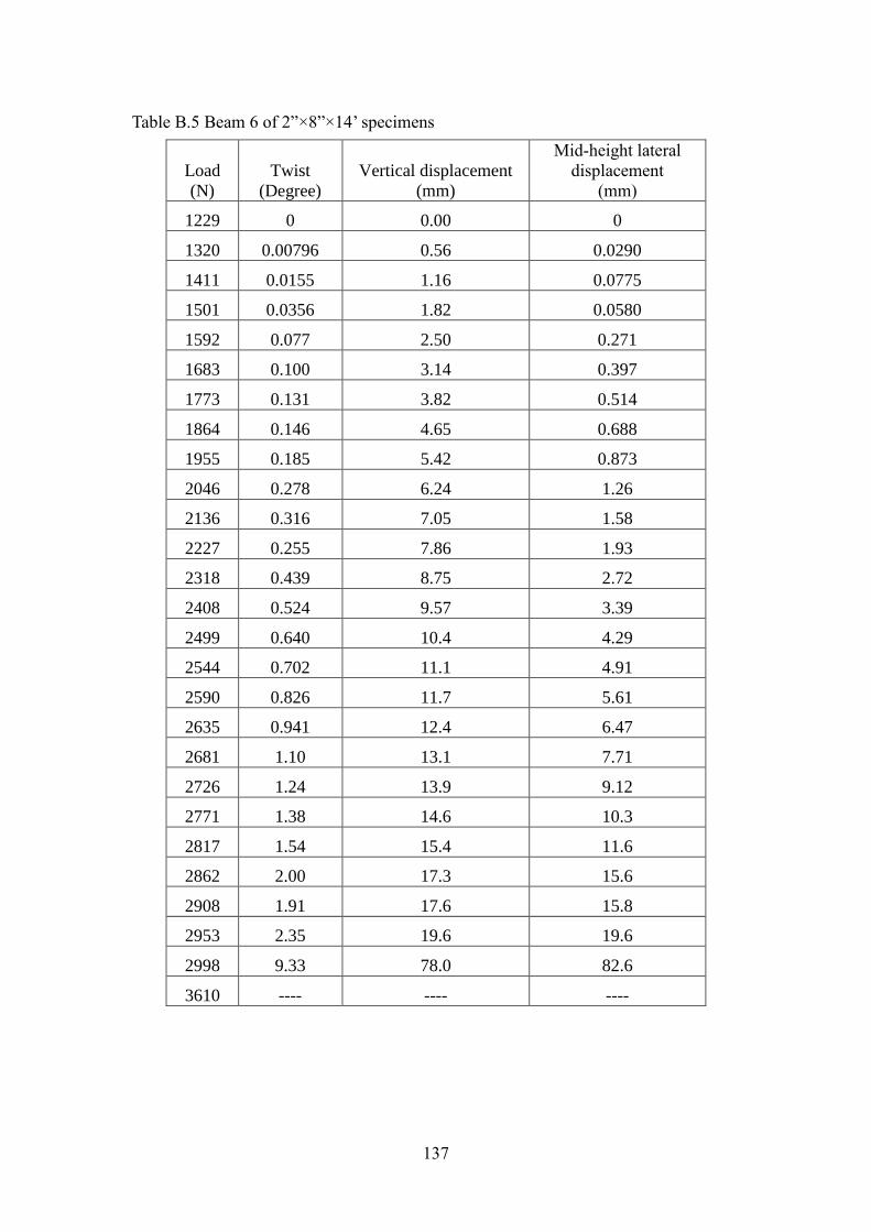
137
Table B.5 Beam 6 of 2”×8”×14’ specimens
Load
(N)
Twist
(Degree)
Vertical displacement
(mm)
Mid-height lateral
displacement
(mm)
1229 0 0.00 0
1320 0.00796 0.56 0.0290
1411 0.0155 1.16 0.0775
1501 0.0356 1.82 0.0580
1592 0.077 2.50 0.271
1683 0.100 3.14 0.397
1773 0.131 3.82 0.514
1864 0.146 4.65 0.688
1955 0.185 5.42 0.873
2046 0.278 6.24 1.26
2136 0.316 7.05 1.58
2227 0.255 7.86 1.93
2318 0.439 8.75 2.72
2408 0.524 9.57 3.39
2499 0.640 10.4 4.29
2544 0.702 11.1 4.91
2590 0.826 11.7 5.61
2635 0.941 12.4 6.47
2681 1.10 13.1 7.71
2726 1.24 13.9 9.12
2771 1.38 14.6 10.3
2817 1.54 15.4 11.6
2862 2.00 17.3 15.6
2908 1.91 17.6 15.8
2953 2.35 19.6 19.6
2998 9.33 78.0 82.6
3610 ---- ---- ----

138
Table B.6 Beam 2 of 2”×10”×12’ specimens
Load
(N)
Twist
(Degree)
Vertical displacement
(mm)
Mid-height lateral
displacement
(mm)
3444 0 0 0
3533 0.034 0.010 0.116
3622 0.199 0.506 1.06
3711 0.205 0.506 1.05
3800 0.177 0.650 1.02
3889 0.182 0.826 1.07
3978 0.182 1.03 1.09
4067 0.193 1.26 1.12
4156 0.194 1.44 1.14
4245 0.182 1.84 1.07
4334 0.205 1.92 1.16
4423 0.216 2.16 1.28
4512 0.233 2.44 1.35
4601 0.245 2.69 1.42
4690 0.234 2.87 1.42
4779 0.233 3.10 1.41
4868 0.228 3.35 1.43
4957 0.239 3.59 1.59
5046 0.313 4.21 2.05
5135 0.347 4.28 2.26
5224 0.353 4.51 2.35
5313 0.410 4.86 2.69
5402 0.444 5.12 2.95
5491 0.467 5.39 3.12
5672 4.35 10.5 24.9

139
Table B.7 Beam 3 of 2”×10”×12’ specimens
Load
(N)
Twist
(Degree)
Vertical displacement
(mm)
Mid-height lateral
displacement
(mm)
1928 0 0 0
2017 0.0059 0.145 0.281
2106 0.0685 0.723 1.07
2195 0.0229 1.02 0.814
2284 0.0737 1.24 1.64
2373 0.310 1.52 3.06
2462 0.367 1.90 4.69
2551 0.524 2.28 6.67
2640 0.688 2.58 8.42
2729 0.928 3.12 11.4
2818 1.27 3.77 14.9
2907 1.60 4.31 18.6
2996 2.29 5.31 25.8
3085 3.19 7.31 36.0
3174 4.36 10.3 46.2
3341 ---- ---- ----

140
Table B.8 Beam 5 of 2”×10”×12’ specimens
Load
(N)
Twist
(Degree)
Vertical displacement
(mm)
Mid-height lateral
displacement
(mm)
3485 0 0 0
3576 0.00588 0.010 0.0290
3667 0.0223 0.217 0.0770
3758 0.0341 0.217 0.116
3848 0.0626 0.372 0.243
3939 0.0629 0.496 0.242
4030 0.0740 0.640 0.339
4120 0.103 0.805 0.485
4211 0.0855 0.940 0.495
4302 0.091 1.07 0.485
4392 0.120 1.26 0.669
4483 0.148 1.40 0.872
4574 0.165 1.59 0.979
4665 0.160 1.70 1.05
4755 0.136 1.91 1.11
4846 0.165 2.04 1.27
4937 0.165 2.23 1.29
5027 0.182 2.34 1.42
5073 0.222 2.35 1.64
5118 0.245 2.57 1.77
5163 0.250 2.59 1.88
5209 0.251 2.79 1.96
5254 0.274 2.80 2.02
5299 0.273 2.80 2.04
5345 0.303 3.01 2.09
5390 0.285 3.02 2.17
5436 0.285 3.19 2.19
5481 0.319 3.24 2.52
5526 0.325 3.25 2.53
5572 0.364 3.41 2.89
5685 0.462 3.57 3.60
5784 0.478 3.59 3.88
5875 0.672 3.99 5.37
5965 0.934 3.99 7.11
6030 0.997 3.97 7.72
6111 1.14 3.97 8.94
6191 1.22 3.98 9.53
6300 ---- ---- ----
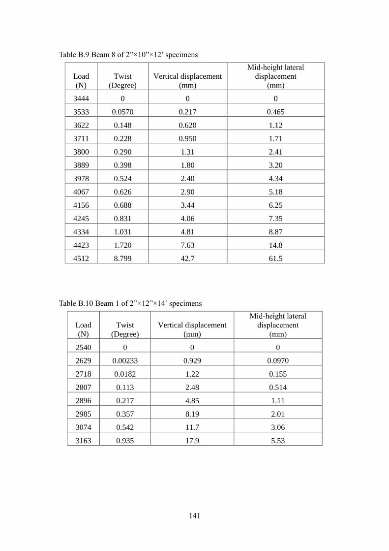
141
Table B.9 Beam 8 of 2”×10”×12’ specimens
Load
(N)
Twist
(Degree)
Vertical displacement
(mm)
Mid-height lateral
displacement
(mm)
3444 0 0 0
3533 0.0570 0.217 0.465
3622 0.148 0.620 1.12
3711 0.228 0.950 1.71
3800 0.290 1.31 2.41
3889 0.398 1.80 3.20
3978 0.524 2.40 4.34
4067 0.626 2.90 5.18
4156 0.688 3.44 6.25
4245 0.831 4.06 7.35
4334 1.031 4.81 8.87
4423 1.720 7.63 14.8
4512 8.799 42.7 61.5
Table B.10 Beam 1 of 2”×12”×14’ specimens
Load
(N)
Twist
(Degree)
Vertical displacement
(mm)
Mid-height lateral
displacement
(mm)
2540 0 0 0
2629 0.00233 0.929 0.0970
2718 0.0182 1.22 0.155
2807 0.113 2.48 0.514
2896 0.217 4.85 1.11
2985 0.357 8.19 2.01
3074 0.542 11.7 3.06
3163 0.935 17.9 5.53

142
Table B.11 Beam 2 of 2”×12”×14’ specimens
Load
(N)
Twist
(Degree)
Vertical displacement
(mm)
Mid-height lateral
displacement
(mm)
1633 0 0 0
1722 0.235 0.0720 1.18
1811 0.375 0.0720 2.06
1900 0.515 0.0310 3.02
1989 0.573 0.134 3.52
2078 0.754 0.238 4.66
2167 0.907 0.314 6.10
2256 1.06 0.475 7.30
2345 1.24 0.712 8.66
2434 1.36 0.878 9.99
2523 1.59 1.04 11.9
2612 1.73 1.24 13.2
2701 1.93 1.71 15.2
2790 2.21 2.12 17.7
2879 2.57 2.54 21.0
2968 2.33 3.02 20.3
3057 2.50 3.46 22.0
3146 3.35 4.99 29.0
3191 4.65 8.13 40.7
3235 5.93 12.7 51.2
3280 6.07 13.9 53.1