Laser profiling of sewer pipes

Laser profiling of sewer pipes

Analysis of concrete egg shaped sewer pipes

Walter van der Schoot

for the degree of:

Master of Science in Civil Engineering

Date of submission: 9 January 2015 Date of defence: 12 February 2015

Committee: Prof.dr.ir. F. Clemens Delft University of Technology Sanitary Engineering Section Dr.ir. J. Langeveld Delft University of Technology

Sanitary Engineering Section Ir. N. Stanic Delft University of Technology

Sanitary Engineering Section Ir. W.M.J. Luxemburg Delft University of Technology Water Resources Section

Sanitary Engineering Section, Department of Water Management Faculty of Civil Engineering and Geosciences Delft University of Technology, Delft

3

4

Abstract Introduction In developed countries like the Netherlands there is an extensive and well functioning sewer system. Over the years 111.000 kilometres of sewer pipes were constructed in the Netherlands. With an effective management proper serviceability of the asset can be achieved on the long-term, which will minimize adverse effects on human health and environment. Moreover, cost-effective sewer asset management is necessary to attain a preferred service level at lowest public costs.

Problem definition To enable effective sewer asset management a reliable source of information has to be available about the state of an asset. Nowadays CCTV inspections and pipe age are the main sources of information about the state of sewer pipes. These techniques don’t always provide conclusive information. Laser profiling is a relatively new technique which can aid to gain information about the state of. A laser profiler, as an adjunct to CCTV, can identify the profile of a sewer and also wall loss from corrosion compared to an assumed initial situation. Research

The goal of the research is to determine the potential of laser scanning methods for accurate, non-invasive assessment of the changes in the inner pipe profile of concrete sewer pipes. The main research question is: ‘How accurate is the laser profiler when measuring deteriorated sewer pipes?’

In the research egg shaped concrete sewer pipes were measured under laboratory conditions. The used experimental setup consists of an old concrete, egg shaped sewer pipe. At the front and back of the pipe a ramp is placed to ensure a smooth entrance and exit of the inspection camera. The recordings from the laser profiler are analyzed with Matlab to determine the accuracy.

Results The accuracy of the laser profiling remained within 0.5% while stationary. However when the camera with the laser profiler is moving through the pipe the accuracy is reduced drastically. In fact when corrected for movement the values deviated up to 15.9mm in one axis. Also an attempt to link the corrosion to the wall thickness was inconclusive due to difference in theoretical and actual shape of the egg shaped sewer pipes. Conclusions and Recommendations It is a technique with potential to deliver 3D information about the inside of a sewer pipe. However for that use the accuracy has to be improved while moving. In the future it can be used to objectify inspection techniques and can be used in sewer renovation. In this process the aspect of determining the remaining wall thickness with laser profiling will always remain difficult due to unknown starting conditions. Student: W.P.J. van der Schoot Committee: Prof.dr.ir. F. Clemens Delft University of Technology Sanitary Engineering Section Dr.ir. J. Langeveld Delft University of Technology

Sanitary Engineering Section Ir. N. Stanic Delft University of Technology

Sanitary Engineering Section Ir. W.M.J. Luxemburg Delft University of Technology Water Resources Section

5

Preface The reason to attend the Master’s study Water Management at the TU Delft is because the sewer is a neglected but very important issue in the Netherlands, or as my friends would explain to me: “My shit is your job”. I started studying civil engineering at the University of Twente, where I received my bachelor’s degree. However, my love for the field of sanitary engineering arose a few years back when I did my internship at the engineering agency MWH in Delft. The subject of my internship was “Asset management as part of sewer management at municipalities”. This was my first acquaintance with sewer management and the subject intrigued me. It lead to an easy decision to continue my Master’s study at the TU Delft on the subject of Water management. After another internship at civil contractor GMB where I constructed new sewers at the Maasvlakte II, I found a suitable thesis topic subject at the sanitary department. The thesis was about testing and measuring the geometry and pipe characteristics of deteriorated concrete sewer pipes. It was a very educational experience which, being executed partly next to my job at GMB has taken much more time to finalise than what was expected. Along the way to the finalisation of my research a lot of people have supported me, All the PhD student were familiar with the research and have contributed somewhere in the process. This is very much appreciated, and I would like to thank them for their input. I like to thank Nikola Stanic for the interesting discussions and input during the thesis. Special thanks goes to Francois Clemens who was my counsellor during the internship and master thesis. Besides the people at the TU Delft, I would also like to acknowledge and thank the companies “Van der Valk en de Groot” for providing the means necessary to execute the experiments. On top of that special thanks to their employees who did a fantastic job enabling all the experiments with their support. Especially Bert Kuier, who helped out with the experiments and contributed extraordinary in the overall process.

6

Content

1 Introduction 7

1.1 A need for sewer asset management 7

1.2 Problem definition 8

1.3 Scope and goal of the research 10

1.4 Structure of the report 10 2 Approach and methods 11

2.1 Used equipment and material 11

2.2 Measuring setup 13

2.3 Experimental method 14

2.4 Measuring uncertainties 14

2.5 Future research 16

2.6 Preparation of the pipes for further experiments 18 2.7 Data Processing 18

3 Results and discussion 24

3.1 Measuring uncertainties 24

3.2 Manual wall thickness measurements. 26

3.3 Measuring variations 28

3.4 Data processing 30 4 Conclusion and recommendations 36

List of references 37

Annexes 39

Annex A Theoretical degradation 39

Annex B Case study characteristics 43

Annex C Dimensions movement measuring device 46

Annex D Article 47

7

1 Introduction

In developed countries like the Netherlands there is an extensive and well functioning sewer system. Over the years 111.000 kilometres of sewer pipes were constructed and 99.8 % of the population is connected to a sewer system. This is in fact the highest percentage of connected households of all the countries of Europe. The performance of the system can be illustrated in by the comparison of the average downtime (time not functioning). The downtime of the sewer system in the Netherlands is only 0.6 minute per household per year. In comparison, the downtime of electricity is 14 minutes per household per year (Feitencommissie, 2010). With time the sewer system deteriorates due to aging, overloading, misuse and mismanagement. The Municipalities in the Netherlands are responsible for the maintenance of the sewer system; they finance the sewer maintenance mostly from the sewer taxes which every household has to pay. With an effective management proper serviceability of the asset can be achieved on the long-term, which will minimize adverse effects on human health and environment. Moreover, cost-effective sewer asset management is necessary to attain a preferred service level at lowest public costs.

1.1 A need for sewer asset management

The main issue is that the sewer maintenance costs have increased over the last 10 years. Urban drainage systems are viewed as a capital intensive infrastructure. For instance, the estimated value of the existing urban drainage infrastructure in the Netherlands is around 77 billion euro’s. To be able to pay for the maintenance of this infrastructure, the total amount of sewer taxes has been doubled between the year 2000 and 2010. In 2010 it was around 1.3 billion euro’s per year. In 2012 the cost already rose to 1.4 billion and it is expected that the costs will increase further to 1.7 billion in the year 2020. The main cause for this increase is the aging of the sewer systems. A total of 88% of the system is constructed after the 1950’s and with an average technical lifespan of around 60 years an increasing part has to be replaced or repaired in the near future (Feitencommissie, 2010). To limit this increase in costs the various actors in the water sector want to increase their efficiency. In order to achieve this The Provinces, The Municipalities, Drinking Water companies and Waterboards joined forces in the commission “Feitenonderzoek” which looked at possible savings in the entire water sector. Their report states that till the year 2020 a saving of 8% in the sewer management is feasible. One of the main pillars to achieve this is the structural application of asset management within the sewer management (Feitencommissie, 2010). However, saying is one thing and doing is another. Asset management is not an exact science and there are many interpretations and definitions available. The one used in this report is the definition according to PAS 55-1:2008: “Systematic and co-ordinated activities and practices through which an organization optimally and sustainably manages its assets and asset systems, their associated performance, risks and expenditures over their life cycles for the purpose of achieving its organizational strategic plan.” (Institution, 15 September 2008) Overall, asset management consists of multiple steps and processes to manage assets. These processes are depicted in Figure 1. The field of interest of this thesis is the determination of objectives, in other words the information needed to make decisions about an asset.

8

Figure 1. Processes in Asset management

Since 1993 the Municipalities are obliged by The Dutch Government to apply asset management (article 4.22, Wet milieubeheer). They have to report their Municipal Sewer Plan (Gemeentelijk Riolerings Plan). The goal of the sewer asset management is to provide optimum decisions on the provision for maintenance, on-going operation and on the provision of the large investments, associated with sewer rehabilitation and replacement. The schematic diagram of the semanagement process is given in Figure 1. The investigation and assessment, the first two stages, are important factors in the sewer system management due to the fact that they have direct impact on all further stages

Figure 1: Schematisation of the sewer system management process (Nederlands Normalisatie-instituut, 2008).

1.2 Problem definition

Today, it is still difficult to assess the actual condition of the sewer pipes. Decisions on rehabilitation and maintenance of sewers should be made based on reliable information on the physical status of the sewer system and on its serviceability. The primary sources of information used in decision making (e.g. necessary replacement) are pipe age and Closed Circuit Television (CCTV) inspections. The difficulty with pipe age is that it is only one of many factors influencing the deterioration of sewer pipes. For example in The Municipalities

. Processes in Asset management

Since 1993 the Municipalities are obliged by The Dutch Government to apply asset Wet milieubeheer). They have to report their actions in the

Municipal Sewer Plan (Gemeentelijk Riolerings Plan).

The goal of the sewer asset management is to provide optimum decisions on the provision for going operation and on the provision of the large investments, associated

with sewer rehabilitation and replacement. The schematic diagram of the sewer system management process is given in Figure 1. The investigation and assessment, the first two stages, are important factors in the sewer system management due to the fact that they have direct impact on all further stages (Nederlands Normalisatie-instituut, 2008).

Figure 1: Schematisation of the sewer system management process (Nederlands

instituut, 2008).

Problem definition

Today, it is still difficult to assess the actual condition of the sewer pipes. Decisions on d maintenance of sewers should be made based on reliable information on

the physical status of the sewer system and on its serviceability. The primary sources of information used in decision making (e.g. necessary replacement) are pipe age and Closed

) inspections. The difficulty with pipe age is that it is only one of many factors influencing the deterioration of sewer pipes. For example in The Municipalities

Thesis’

Since 1993 the Municipalities are obliged by The Dutch Government to apply asset actions in the

The goal of the sewer asset management is to provide optimum decisions on the provision for going operation and on the provision of the large investments, associated

wer system management process is given in Figure 1. The investigation and assessment, the first two stages, are important factors in the sewer system management due to the fact that they have

Figure 1: Schematisation of the sewer system management process (Nederlands

Today, it is still difficult to assess the actual condition of the sewer pipes. Decisions on d maintenance of sewers should be made based on reliable information on

the physical status of the sewer system and on its serviceability. The primary sources of information used in decision making (e.g. necessary replacement) are pipe age and Closed

) inspections. The difficulty with pipe age is that it is only one of many factors influencing the deterioration of sewer pipes. For example in The Municipalities

Thesis’ Field of interest

9

with soft soil the sewer system has to be replaced more often than in municipalities which are located on solid soils. The setting of the soft soil influences the service life of the sewer pipes more than the pipe age. A few other factors that influence the service life are the installation method, surface use, groundwater level and section length influence the deterioration. In conclusion, information on the pipe age is insufficient to provide knowledge on the actual condition of the sewer pipes. The visual inspection with CCTV has disadvantages as well. Recent research of Dirksen et. al., (2011) shows that there are inconsistencies in the assessment of the visual data from CCTV inspections. In the research the same stretch of pipe was assessed by different qualified inspectors and the assessment of the recorded damages differed per person. This could mean that in some cases the municipality would replace the pipe and in another case they wouldn’t. Even so with severe damage to the pipe or obvious clogging the CCTV inspections will give a conclusive answer. Overall, research shows that the quality of visual inspection data is insufficient to make proper decisions about sewer renewal. In order to overcome the limitations of visual inspection, several new techniques have been developed over the past two decades and are applied in practice, like radar (e.g. Olhoeft, 2000), acoustic techniques (e.g. Feng, Horoshenkov, Tareq, & Tait, 2012), sonar (Kirkham et al., 2000), or laser profiling (Duran, Althoefer, & Seneviratne, 2003). Laser profiling of (sewer) pipes is a technology that is introduced and applied in practice for some years. A laser profiler, as an adjunct to CCTV, can identify the profile of a circular sewer and also wall loss from corrosion (Thomson et al., 2010). Some research claim that the laser profiling technique is capable of measuring the wall losses due to corrosion (Kirkham et al., 2000) with a relative uncertainty of 0.5%. However, Duran et al. (2003) state that the main difficulty in laser profiling is the alignment and orientation of the sensor in the harsh sewer environment. In summation, to authors’ knowledge no attempt to measure actual pipe wall thickness of deteriorated sewer pipe was reported so far, as well as to quantify uncertainties related to the laser profiling inspection technique. For the aforementioned reasons, further studies need to be carried out in order to fill the gap of previously carried out research and provide reliable information on the condition of the sewer assets.

10

1.3 Scope and goal of the research

This thesis is part of a PhD research which aims at a better understanding and gaining advanced knowledge on the collapse of deteriorated sewer pipes. Part of the PhD research is to determine physical and structural properties of deteriorated concrete sewer pipes. With this data a model for the probability of pipe collapse can be created, which will contribute to better estimate the probability of collapse of sewer pipes. Consequently, if the remaining life span of concrete sewer pipes can be predicted better than based on CCTV inspections and pipe age, the investments associated with sewer rehabilitation and replacement can be optimized even further. Input for the numerical model in the PhD will be the pipe dimensions and material characteristics, or summarized, the following data will be collected:

1. Dimensions of the pipe/the remaining wall thickness

2. Determine the characteristics of the material o Crushing strength - Cracking the pipes o Material properties - Drill core analysis

3. Numerical model

The goal of this research is to determine the potential of laser scanning methods for accurate, non-invasive assessment of the changes in the inner pipe profile of concrete sewer pipes. The main research question is: ‘How accurate is the laser profiler when measuring deteriorated sewer pipes?’ The detailed objectives of the research are:

• To quantify measuring uncertainties. • To measure the shape of the pipe interior and exterior. • To post-process raw data in Matlab platform.

1.4 Structure of the report This introduction chapter describes the context of sewer asset management and current sources of information used in decision making. It identifies a number of shortcomings in existing approaches and addresses some. . Chapter 2 describes the used equipment materials and methodology. Chapter 3 sums up the results in graphs and tables together with a discussion of it. At the end of the thesis the summary and conclusions of this study are presented. Furthermore, in the annexes background information can be found about the process of deterioration of concrete sewer pipes, as well as information on the original location of the used pipes.

1. Pipe Geometry2. Material

characteristics3. Numerical model

11

2 Approach and methods

2.1 Used equipment and material

Sewer pipes

In the research, egg shaped sewer pipes are used with dimensions 300/450 mm and 400/600 mm, the regular shape is shown in Figure 2. The pipes come from regular sewer renovation projects in the Hague and Breda. The location and properties of the pipe, such as years in service, ground water level and soil type are recorded for both locations in Table 1 and described in detail in annex B. Table 1. General characteristics of the studied sewer pipes

Characteristic Breda The Hague

Years in service Groundwater level (m) Soil type Surface load Inspection results

61 Mostly above invert level Peat, clay, sand 35 years of high traffic load Surface damage BAF 3

89 Below invert level Sand Only domestic Surface damage class BAF 4

A detailed characteristic of each studied pipe is given in Table 2.Prior to excavation visual inspections were performed to determine the condition of the inner surface of the sewer i.e. surface damage by internal chemical (corrosion) or mechanical action (code BAF). The registration of defects was done according to the visual inspection coding Standard NEN-EN 13508-2, while the Standard NEN 3399 was used to assign a level of severity to each defect – condition assessment (Nederlands Normalisatie-instituut 2003; 2004a). Table 2. Deterioration characteristics based on sewer inspection prior to excavation of the sewer pipes. Defects are reported based on the coding from NEN 3399.

No. Origin Year of

construction

Surface

damage class

(BAF)

BAF class

description

1 De Hamer factory new - 2 The Hague 1924 4 Missing aggregates or

reinforcement outside the surface protrudes

3 The Hague 1924 4

4 Breda 1952 3 Aggregates that protrude beyond the surface or visible reinforcement

5 Breda 1952 3

Panoramo camera

During the research the sewer pipe conditions were assessed using the IBAK PANORAMO camera system/optoscanner, a relatively new concept in the field of pipeline inspection (Figure 3). The IBAK PANORAMO 360 utilizes two high-resolution, 186°, wide-angle camera lenses to captures a complete, 360° spherical image of the pipe. The video recording can be unfolded and assessed in real time or at a later date and permits computer-aided measurement of the positions and sizes of objects or pipe defects. Furthermore, the system

400 mm

600 mm

Figure 2. Illustration of the general shape of an Egg shaped sewer pipe. The dimensions of the used pipes in the research are depicted (400mm / 600mm)

12

has no external moving parts - hence it is robust and has less chance to fail; the captured images are always sharp, regardless of the recording.

Laser profiler The change in shape of the sewer pipe interior was assessed by a concept employing a CLEARFLOW Clearline laser profiler coupled to a PANORAMO optoscanner (Figure 5). A laser profiler, as an addition to the camera, can identify the profile of a pipe and also wall loss from corrosion (Thomson et al., 2010). The laser profiler mode of operation is based on a laser ring, which is projected onto the pipe wall and subsequently recorded by the connected camera. Figure 4shows the principle of the laser based inspection concept.

The laser profiler mode of operation is based on a laser ring, which is projected onto the pipe wall and subsequently recorded by the connected camera (Figure 7). The software calculates the data received and creates a 3D model of the pipe geometry. As an illustration an image of a round pipe is shown in Figure 6.

Figure 3. Panoramo camera system for sewer inspections, dimensions and overall view of the device.

Figure 4. Principle of the laser profiler, the projected laser is recorded by the sewer inspection camera.

Figure 5. Panoramo camera head with the laser emitter of the Clearflow Clearline laser profiler attached to it.

Figure 6. Example of general Laser profiler output from Clearflow Clearline software, it shows the locations, on top of the pipe, where the recorded diameter is larger than the pipe.

Figure 7. An actual frame from the recording of the Panoramo camera with the laser profiler. This shows how the laser is recorded, although normally in the dark.

13

2.2 Measuring setup

The experimental setup (Figure 8) consists of an old concrete, egg shaped sewer pipe. At the front and back of the pipe a ramp is placed to ensure a smooth entrance and exit of the inspection camera. With a frame over these ramps the setup is darkened to ensure good visibility of the laser. As described the profiler projects a laser ring on the pipe wall that is captured by the camera and identifies the shape of the pipe interior.

Figure 8. Measuring setup which is used to perform the measurements. To create situations comparable to the sewer the setup is covered with a large black plastic film.

Secondly, the shape of the pipe exterior was determined by measuring the wall thickness at 4 selected locations on both ends of the pipe (Figure 9). This was done with a calliper gauge and a frame clamp. Cylinder-shaped objects were used as indicators of the selected location for the measurements.

Width

1

Height 2 4

3

Front view Side view

Length

FS1

FS2/4

FS3

BS1

BS2/4

BS3

Length

Front Back

Length

Figure 9. in each pipe several reference shapes are placed for measurements. The locations of the reference shapes have a unique coded and in total eight locations shapes are placed per pipe.

14

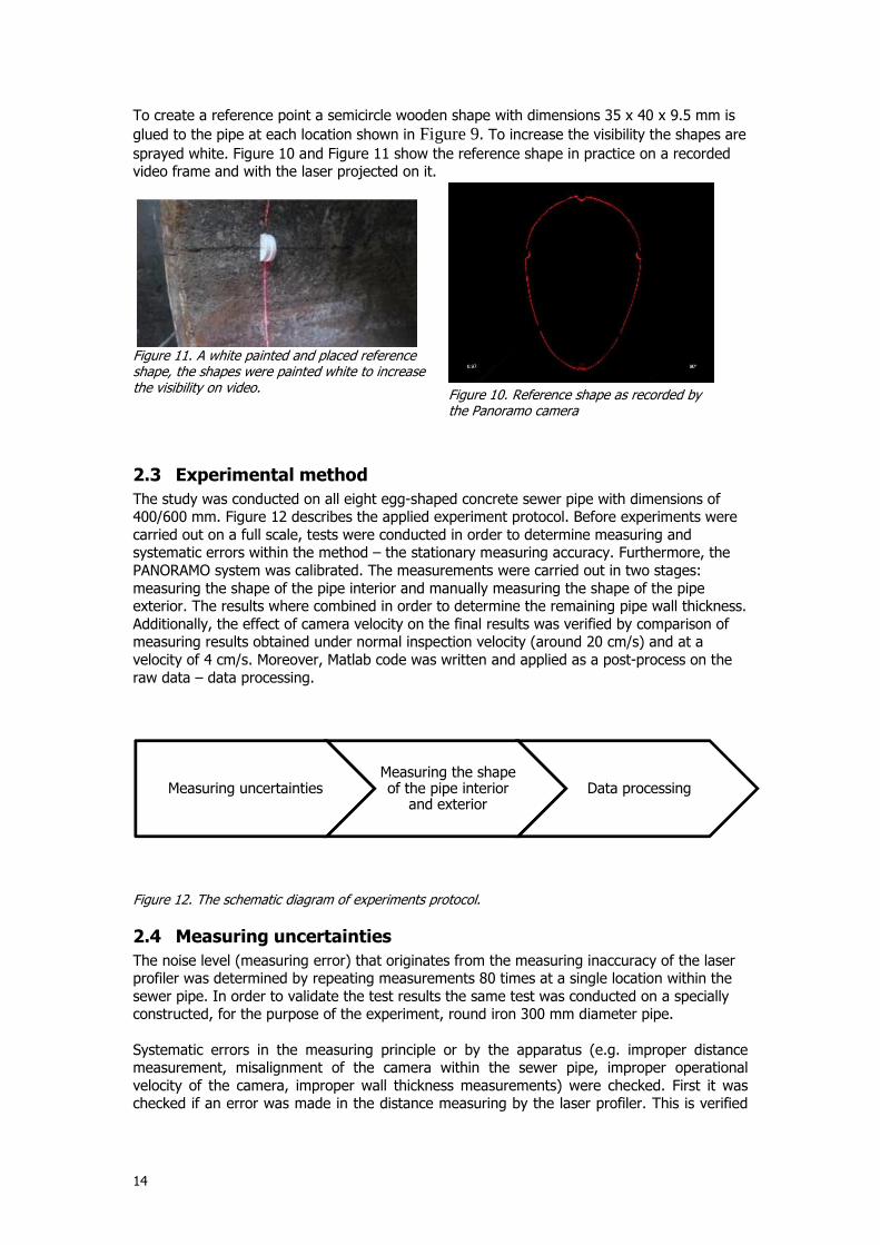
To create a reference point a semicircle wooden shape with dimensions 35 x 40 x 9.5 mm is

glued to the pipe at each location shown in Figure 9. To increase the visibility the shapes are

sprayed white. Figure 10 and Figure 11 show the reference shape in practice on a recorded video frame and with the laser projected on it.

Figure 11. A white painted and placed reference shape, the shapes were painted white to increase the visibility on video.

2.3 Experimental method

The study was conducted on all eight egg-shaped concrete sewer pipe with dimensions of 400/600 mm. Figure 12 describes the applied experiment protocol. Before experiments were carried out on a full scale, tests were conducted in order to determine measuring and systematic errors within the method – the stationary measuring accuracy. Furthermore, the PANORAMO system was calibrated. The measurements were carried out in two stages: measuring the shape of the pipe interior and manually measuring the shape of the pipe exterior. The results where combined in order to determine the remaining pipe wall thickness. Additionally, the effect of camera velocity on the final results was verified by comparison of measuring results obtained under normal inspection velocity (around 20 cm/s) and at a velocity of 4 cm/s. Moreover, Matlab code was written and applied as a post-process on the raw data – data processing.

Figure 12. The schematic diagram of experiments protocol.

2.4 Measuring uncertainties

The noise level (measuring error) that originates from the measuring inaccuracy of the laser profiler was determined by repeating measurements 80 times at a single location within the sewer pipe. In order to validate the test results the same test was conducted on a specially constructed, for the purpose of the experiment, round iron 300 mm diameter pipe. Systematic errors in the measuring principle or by the apparatus (e.g. improper distance measurement, misalignment of the camera within the sewer pipe, improper operational velocity of the camera, improper wall thickness measurements) were checked. First it was checked if an error was made in the distance measuring by the laser profiler. This is verified

Measuring uncertaintiesMeasuring the shape of the pipe interior

and exteriorData processing

Figure 10. Reference shape as recorded by the Panoramo camera

15

using a simple laser distance meter at the exact location where the profiler projects its laser beam at the reference locations described in 2.2. Due to an uneven surface of the pipe and possible freedom of movement of camera misalignment can occur along the vertical and horizontal axis. The amount of error due to misalignment was quantified by mathematical calculations. At each reference location the wall thickness is measured manually as a reference location to link the inside and outside of each pipe. Errors caused by human error during the measuring process of wall thickness were checked by re-measuring. The measuring accuracy is defined as the 95% accuracy interval (4σ).

16

2.5 Future research

Results from the previously described measurements showed that movement of the camera influences the measurements. A setup to determine the uncertainties due to movement during measurements was created as a part of further research comprising all the uncertainties associated with the laser profiler. The research is described in the published article: “Uncertainties associated with laser profiling of concrete sewer pipes for the quantification of the interior geometry “(Clemens, Stanić, Van der Schoot, Langeveld, & Lepot, 2014). Measurements for this article are executed as part of this thesis. The software to analyse the pixel intensity on page 4 and 5 of the article is developed during the thesis and the setup to measure the movement as well. The measuring setup is developed during the thesis together with Francois Clemens and Nikola Stanic. Measuring setup for measurements with moving camera

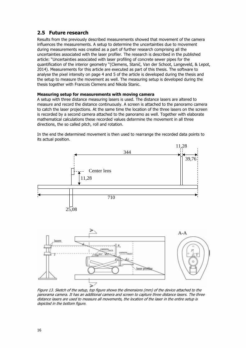
A setup with three distance measuring lasers is used. The distance lasers are altered to measure and record the distance continuously. A screen is attached to the panoramo camera to catch the laser projections. At the same time the location of the three lasers on the screen is recorded by a second camera attached to the panoramo as well. Together with elaborate mathematical calculations these recorded values determine the movement in all three directions, the so called pitch, roll and rotation. In the end the determined movement is then used to rearrange the recorded data points to its actual position.

Figure 13. Sketch of the setup, top figure shows the dimensions (mm) of the device attached to the panorama camera. It has an additional camera and screen to capture three distance lasers. The three distance lasers are used to measure all movements, the location of the laser in the entire setup is depicted in the bottom figure.

25,08

39,76

11,28 344

710

11,28

Center lens

17

Figure 14. Actual photographs of the entire setup with additional camera, as showed in figure 13.

Aligning the lasers An important step to reduce uncertainties is the alignment of the three lasers. To align the three lasers a board with mm paper is put thirty meters away from the lasers. With small adjustments to the setup each laser is aimed at the same point as where it should be when the board is put in front of the three lasers. At first this is done in the hallway, Figure 15 but at the v.d. Valk company a special straight line is used to align the inspection camera. This line is used to align the lasers before executing the measurements. With this method a deviation of +/- 3 mm in thirty meters was achieved, based on the mm paper.

Figure 15. These photographs give an indication of the process to align the three lasers, the photographs are taken in the hallway of an apartment building.

18

2.6 Preparation of the pipes for further experiments

Besides the reference points and the manual measurement, each pipe is photographed for analyses in the future. With these photographs any abnormalities at the inside of the pipe might be linked to the outside of the pipe. To create a complete image of each pipe, six

pictures are taken, as an illustration the pictures of one pipe are depicted in Figure 16.

Figure 16. Of each pipe six photographs are taken to record the outside and inside of each pipe. The photographs shown are from pipe number one, the house number was painted on each pipe when excavated to determine the location.

After the pictures are taken, the pipes are painted in three colours and numbered square planes(Figure 17). These colours show the crown, side and invert level of the pipe. At the same time the numbers in the squares determine the position along the length of it. This is done to make the pipes ready for further analysis with drill cores and to create a link between the inside and outside of the pipe, but this is out of the scope of the thesis report.

Figure 17. A pipe before and after painting for future research, the colors depict the crown, side and invert level, each square is numbered to create a specific location on each pipe.

19

2.7 Data processing The raw data need to be processed to obtain the information sought after. Although the laser profiler comes with a software programme it was necessary to write a Matlab code, because the original software does not support egg-shaped sewer pipes nor produces enough data points. The full Matlab scripts are available on request. Instead the process is described and illustrated based on eight different steps. The data processing encompasses the following steps: Step 1

Firstly, an avi video is recorded with the PANORAMO system. Figure 18 shows a single

frame/image from one of the video’s.

Figure 18. Step 1: Original frame from a measurement with the

laser profiler, recorded with the panorama camera.

Step 2

Determine the x, y position of the laser projection from the recorded image using Matlab.

Figure 19. Step 2:The data points obtained from the frame with Matlab,

the blanks are missing data points.

20

Step 3

Further, interruptions in the laser signal due to unevenly deteriorated pipe surface occurred, and these gaps were filled in with interpolation technique. Linear interpolation was adopted due to small interruptions in the signal. The code filled in the gaps if the distance was more than the average distance between the measured points. This comes down to every 2.4 pixel, which corresponds to an average distance of 2.2 mm.

Figure 20. Step 3:Interpolation is used to fill in the gaps.

Step 4 The loss of wall thickness can be quantified by overlapping the measured and theoretical profile of the pipe. Therefore, a theoretical profile of the pipe is created, based on the dimensions defined by Standard NEN 7126. In this step mm to pixel factor is added in order to correctly scale the theoretical pipe profile. This factor is determined during PANORAMO system calibration.

Figure 21. Step 4: A perfect theoretical pipe is used as a reference

shape to determine corrosion.

21

Step 5

Due to an uneven surface of the pipe and possible freedom of movement of camera misalignment can occur along the vertical and horizontal axis. In order to correct for these movements during recording and to be able to compare the theoretical pipe with the recorded one, the recorded profile is repositioned in several steps:

5.1

Based on the location of the centre point of the values the data set is moved in the axis system towards the centre of the perfect profile.

Figure 22. Step 5.1: The recorded image is placed over the perfect pipe, the shift is based on the centre point of each pipe. Consequently the area between the boundaries is used to rotate the recorded image for a better fit.

5.2

Furthermore. there is still the problem of rotation - roll and translation in x direction. This is corrected by fitting two circles within the boundaries as shown in Figure 22. Based on the location of the centre points of these two circles the dataset is rotated and moved along the x-axis. This process is iterated twice by the Matlab code in order to correct translation in x direction and rotation.

Figure 23. Step 5.2: Two circles are fitted through the data points

between the boundaries from figure 22. The centre points of these

circles are used for correcting rotation.

22

5.3

At the end, the measured profile needs to be properly fitted to the theoretical one. Errors in vertical positioning will lead to wrong estimation of loss of wall thickness. Any translation in the y direction is corrected using two fitted polynomial equations through the invert level of the perfect pipe and the imperfect pipes’ data set.

Figure 24. Step 5: This is the initial fit before any correction for rotation and vertical movement. The figure shows the data points from perfect pipe and the recorded one.

Figure 25. Step 5:The final result after correcting for movement and rotation. The difference between the perfect and recorded pipe is used to determine the wall loss.

Step 6 The loss of wall thickness is quantified by determining the shortest distance between the theoretical and measured profile for each point.

23

Step 7

At the end, a contour figure of the whole pipe is created based on obtained results from the Matlab code, the measured length between reference shapes and the number of frames in each video.

Figure 26. Step 7: Example of a cut-out from pipe one, a

darker colour means less corrosion. The length of the pipe

is along the y-axis and the perimeter is along the x axis.

The middle of the invert level is at x =o.

Step 8 In addition, a contour figure is created that shows which points are created by interpolation and which ones are the measured points.

Figure 27. Step 8: Example of the origin of data points in the cut-out

from pipe one (Figure 26) the black dots are the added data points.

24

3 Results and discussion

3.1 Measuring uncertainties

Multiple measurements at the same location

Several stationary measurements are executed to get a first indication about the accuracy of the laser profiling. One setup with a smooth iron tube, diameter 300mm, and one setup with a deteriorated egg shape sewer pipe, dimensions 400/600mm. In each setup a location is recorded about eighty times to determine the variation in the data while stationary. The measured values consist of the radius recorded by the laser profiler in combination with the original laser profiler software. As an indication for the accuracy the standard deviation is calculated for each data point, based on the values during the recording. Table 3 shows the values for the perfect round pipe. And table 4 the values for the deteriorated egg shaped pipe. Table 3. Standard deviation and relative error while performing a stationary measurement in a round ø 300mm pipe

Measurement 1 2 3

Processed points - 165 170 172 Times measured - 81 81 42 Average value r mm 150.0833 150.0292 150.2850 Average standard deviation mm 0.4949 0.4290 0.1845 Smallest standard deviation mm 0.1706 0.1613 0.0799 Largest standard deviation mm 2.1508 1.3456 0.3957 Average relative error % 0.3297 0.2860 0.1228 Smallest relative error % 0.1137 0.1075 0.0531 Largest relative error % 1.4331 0.8969 0.2633 In total four stationary measurements are executed in the egg shaped pipe. Measurement one and two are executed at the front and measurement three and four at the back of the pipe. Table 4. Standard deviation and relative error while performing a stationary measurement in an egg shaped concrete sewer pipe

Measurement 1 2 3 4

Processed points - 131 135 137 136 Times measured - 84 96 76 92 Average value D mm 240.1926 239.0891 241.2223 241.2878 Average standard deviation mm 1.3062 1.2837 0.7808 0.8263 Smallest standard deviation mm 0.5244 0.6260 0.3505 0.3725 Largest standard deviation mm 3.1990 3.0053 1.6980 1.6650 Average relative error % 0.5438 0.5369 0.3237 0.3424 Smallest relative error % 0.2183 0.2618 0.1453 0.1544 Largest relative error % 1.3318 1.2570 0.7039 0.6901 The first striking difference is the number of data points recorded. While at the perfect round pipe around 170 data points are recorded per measurement, the deteriorated sewer pipe records only around 135 data points per measurement. This is a reduction of 20 percent, despite that the diameter of the sewer pipe is larger. In fact this comes down to, on average, a data point every 11,8mm in the sewer pipe compared to one every 5,5 mm in the iron pipe. This implies that the reflection influences the amount of data points being recorded.

25

The second distinct result is the difference in relative error. In the sewer pipe measurements one and two are executed at the front and measurements three and four at the back of the pipe. Although the measurement at the back of the sewer pipe have the same relative error as the iron pipe (around 0.3 %), measurements one and two have a larger relative error (around 0.5%). To put this in perspective, this is a reduction of 40% in the relative error even though the way of measuring didn’t change, only the location. The location of the camera with laser profiler during the first two measurements was outside the pipe due to the relative short length of the pipe(1m). During these measurements outside the pipe, the IBAK panorama camera did not yet enter the pipe, but was still placed on a wooden support structure, which causes some vibrations. However the second two measurements are executed in the pipe itself, this might have been a more stable base. The described difference can indicate that small vibrations may already have a relatively large effect on the measurements. In short: the number of recorded data points decreased with 20% and the error expressed as standard deviation is small, but is influenced easily with a change of 40% between the same kind of measurements. Comparing the measured distance with laser profiler values

The distance between reference shapes is measured manually with a laser distance meter and with the laser profiler, table 5 shows the results of these measurements. The measurement is performed several times, however the results from this measurement are not conclusive. Table 5. Comparison between distances measured with laser profiler and distance laser

Vertical Distance

Horizontal Distance

Measured with laser (mm) # 581 380,7

Profiler (mm) 1 578,03 377,79

Profiler (mm) 2 577,77 379,33

diff(%) 1 0,51 0,77

2 0,56 0,36

diff(abs) 1 -2,97 -2,91

2 -3,23 -1,37 The measurements show a difference between the measurement with the laser distance recorder and the values from the laser profiler. Unfortunately the accuracy of the measuring device was more than the half percent difference recorded in the experiment. On top of that, the values obtained from the software can be influenced easily. The values depend on manual input for the diameter, and this is based on the calibration video.

26

3.2 Manual wall thickness measurements.

The wall thickness is measured at four locations in the ten pipes available. In the end not all pipes are used for further research. Manually measuring was a painstaking and long effort but in the end rewarding, because the results are not as expected. The difference in wall thickness at the top and sides, as well as the difference between the pipes from Breda and the Hague are quite interesting.

Figure 28. manually measured wall thickness in the pipes from Breda, measured at the front (white bars) and at the back (black bars).

Figure 29. Manually Measured wall thickness in the pipes from The Hague, measured at the front (white bars) and at the back (black bars).

There are hardly any differences in values between pipes which come from the same location. Figure 29 shows the average values for 400/600 mm pipes from the Hague and Figure 28 the average values from Breda. The values at the front and at the back show small difference.

However comparing the pipes per location shows differences in measured values. This is illustrated in Figure 30, which shows that the wall thickness of the pipes from Breda are less than those from The Hague. Not a big difference, but still a difference while the pipes from the Hague has been in service for almost thirty years more.

27

This can be explained because there are local differences which can influence the state of the pipes, these differences are described in annex A. The recorded difference in wall thicknesses emphasises the role of local influences on deterioration in concrete sewer pipes. It also satisfies the idea that pipe age in itself is not a good indicator for the state of a concrete sewer pipe.

Figure 30. Manually measured wall thickness the Hague (white bars) vs. Breda (black bars).

Another unexpected result, based on these measurements, is the large wall thickness at the top of all the measured pipes. It is not abnormal but, according to the described deterioration process (annex B), under normal conditions corrosion would take place as well at the sides as at the top. So when the deterioration would progress normally the corrosion should be comparable at the sides and top, while in the measurements the wall thickness is significantly larger at the top. A possible explanation is found in the measuring method and the construction of the pipes. When measuring the wall thickness, it was exactly at the top. The top itself was not a smooth circle but more at an angle, this might have increased the measured values. Also based on the age of the pipe the construction took place in 1952 and 1924. Back then the construction was on site and with a template which was not standardized. As a consequence the shape itself depends on the person who constructed the pipe itself. Even nowadays the dimensions are standardized but still variations in wall thickness are accepted, for example the NEN 7126 allows a tolerance between -4,4 mm and +6,8 mm of the nominal wall thickness in new 400/600mm egg shaped sewer pipes.

28

3.3 Measuring variations

Distance and number of frames The created cut-out and origin image of pipe P1 consist of 52 frames which are evenly distributed over the distance between the reference points in the pipe, which is 796mm. At the same time pipe P2 consists of 73 frames evenly distributed over a distance of 826mm. The resulting distance between frames, or as you might state the density of the data points along the length of the pipe (vertical axis in the cut-outs) varies between 15,3 mm and 11,3 mm. This discussion is based on the number of frames, distance between reference points and the corresponding average speed of the panoramo camera with laser profiler. In this case the average speed is calculated based on the measured distance between reference points, frames per second and the number of recorded frames between the reference shapes. As is visible in the graphs there is a very large difference in measuring speed and number of frames while the distance between reference shapes is more or less the same for every pipe. This comes down to a variation in average moving speed between 25 and 5 centimetres per second. The variation in the number of frames lies between 50 and 200 frames. If evenly distributed over the distance between reference points this comes down to a variation in distance between frames of 5mm to 23mm.

Figure 31. Average distance (y-axis) between frames along the length of a pipe. In total 30 measurements (x-axis) are executed and displayed. The horizontal line shows the average distance in mm between frames during all measurements

29

Figure 32.The average speed (y-axis) during the measurements. In total 30 measurements (x axis) are executed and displayed. The horizontal line shows the average speed during all measurements

These large variations in distance between frames and measuring speed makes it hard to compare the measurements. Unfortunately this became apparent after the measurements. The cause for these large variations lies in the used measuring equipment. Moreover the panoramo camera system is developed for practical use in sewers, where the operating speed is not an issue. The device is not build to accurately keep a constant speed during measurements. In fact the speed is regulated by hand with a small joystick.

30

3.4 Data processing

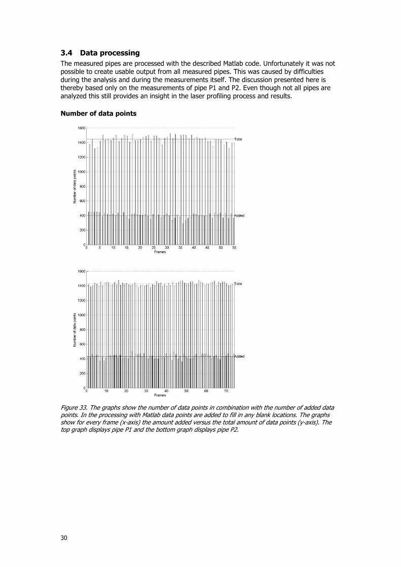
The measured pipes are processed with the described Matlab code. Unfortunately it was not possible to create usable output from all measured pipes. This was caused by difficulties during the analysis and during the measurements itself. The discussion presented here is thereby based only on the measurements of pipe P1 and P2. Even though not all pipes are analyzed this still provides an insight in the laser profiling process and results.

Number of data points

Figure 33. The graphs show the number of data points in combination with the number of added data points. In the processing with Matlab data points are added to fill in any blank locations. The graphs show for every frame (x-axis) the amount added versus the total amount of data points (y-axis). The top graph displays pipe P1 and the bottom graph displays pipe P2.

31

Figure 34. The graphs show the percentage of added data points. In the processing with Matlab data points are added to fill in any blank locations. The graphs show for every frame (x-axis) the percentage of added versus data points compared to the total amount of data points. The top graph displays pipe P1 and the bottom graph displays pipe P2.

The number of data point per frame in each pipe is more or less the same, around 1400 in every frame. The amount of data points added shows similar numbers with around 400 data points added per frame. To elaborate on this , with an estimated perimeter of 1600mm in the sewer pipe there is a data point every 1,1 mm, which allows a detailed picture of the inner surface of the sewer pipe. On the contrary, the fact that 30% of the data points are added by the interpolation indicates that 30 % of the inner surface is not recorded. Of course there is a part that prevents the camera from recording the entire laser projection. The mounting frame of the laser profiler itself, which holds the laser emitter, is always in the recording. Figure 7 and 18 show this. Furthermore the exact distribution of the data points along the perimeter isn’t investigated, the interpolation software/code creates an even distribution of data points on locations where the initial distance is too large. But how this exactly distributes the data points along the perimeter is not certain. Taking this into account it might be a preliminary conclusion but the average adding of 30% of the data points does show that not the entire perimeter of the pipe can be recorded. The reason for this might be bad reflection or just the laser disappearing out of sight behind large concrete aggregate at heavily deteriorated positions.

32

Movement during measurements

The difficulties with processing the data are movements during the measurements. All recorded videos show leaps and shocks in the recordings. As an example, Figure 35 illustrates the movement between frame 172 and 182 of pipe 7. The figure combines the two frames with two equally sized white rectangles. The recorded red laser projections should remain at the same position. This is however clearly not the case. Another indication of the movement during measurements is found in the black and white figures (Figure 36 and 37) which show the origin of data points (original vs. Added) shows signs of these disturbances as well. If the movement was constant and smooth the two black lines (added data points) would be more or less straight. However this might also be caused by the processing of the data with Matlab, but at the same time the processing steps are the same for every frame. Corrosion / Remaining wall thickness

As described in 2.7 the corrosion in the cut-outs is based on the comparison of the measured recorded pipe wall with a theoretical perfect egg shaped pipe. The figures 36 and 37 show the most deterioration at the top and sides of the pipe. This does coincide with the theory as described in Annex A. The manual wall thickness measurements showed that the exterior shape of the egg shaped sewer pipe differs from the theoretical egg shaped sewer pipe. Based on this an accurate estimation the remaining wall thickness is impossible. At least not without additional information on the exterior shape of the pipe to create a link between the in- and exterior of the pipes. For the experimental measurements the pipes are accessible and this link might be created with wall thickness measurements. But especially when the pipes are still in the ground there is no cost efficient option to determine the outer shape of an egg shaped sewer pipe. On the other hands the described issue with the exterior shape of the egg shaped concrete sewer pipes might be less with round pipes. Due to the simpler shape of these pipes the exterior will be more similar than those of the egg shaped sewer pipes. However round sewer pipes are out of the scope of this thesis.

Figure 35. A graphic display of movement during measurements. The figure shows two frames from one video. If the recorded laser is exactly stable both frames should be on the same location.

33

Figure 36. Top figure: cut-out from pipe P1, a darker colour means less corrosion. The length of the pipe is along the y-axis and the perimeter is along the x axis. The middle of the invert level is at t x =o. Bottom figure: Example of the origin of data points in the cut-out from pipe two. The black dots are the added data points.

34

Figure 37.Top figure: cut-out from pipe P2, a darker colour means less corrosion. The length of the pipe is along the y-axis and the perimeter is along the x axis. The middle of the invert level is at t x =o. Bottom figure: Example of the origin of data points in the cut-out from pipe two. The black dots are the added data points.

35

Further research

In the article (Annex E) an analysis for all uncertainties is performed and the recorded data is corrected for movement during measurements. The measurements from the article are performed with the setup developed during this thesis. Afterwards, with a much more powerful computer, the recordings are corrected for movement during the measurements. As shown in Figure 38. The correction can count for as much as 15.9 mm in one axis (Clemens et al., 2014). In this figure 38, the lighter the area, the more deterioration is measured. The corrected version (bottom figure) shows much less deterioration and also at a different location. This shows that the movement during the measurements caused a difference in the spatial distribution of the deterioration and a difference in the amount of deterioration.

Figure 38. Image from the article (Clemens et al., 2014) it shows an cut-out uncorrected (top) for movement and corrected (bottom) for movement. An important difference is that the correction in this image is performed with actual measured movements, while the correction for movement in the cut-outs from figure 36 and 37 are only based on the corrections in the Matlab code.

36

4 Conclusion and recommendations

As a reminder, the main research question is:

‘How accurate is the laser profiler when measuring deteriorated sewer pipes?’ Even though there is no conclusive answer on that main question, the research gives an estimation and showed a clear difference between stationary measurements and measurements while moving. Accuracy

While stationary the accuracy of the measurements with the laser profiler remained within the 0.5% error as stated by the manufacturer. However during measurements with the moving profiler, variations in speed, vibrations and shocks disturbed the recordings. Although these influences were mainly caused by the used set up of the testing equipment it is to be expected that these kind of movements will occur in practice as well. During the research these disturbances resulted in unusable data and caused unpredictable and inaccurate results. Just as in the experiments the recorded movements will influence recordings in practice in the same manner. Therefore to create a correct image of the inner perimeter of a sewer pipe these motions have to be measured and analyzed. Rearranging the recorded data points using positioning measurements will result in a more accurate image. To emphasize this. correcting the data showed that the location of data points might deviate up to 15.9 mm in one axis’ direction. Remaining wall thickness

Some problems arise if laser profiling is used for the purpose of determining the remaining wall thickness in comparison with the original wall thickness of an old concrete sewer pipe. The main problem is that for old pipes the wall thickness at the moment of construction is unknown. Due to the fact that the used pipes are egg shaped this aspect showed to be a crucial uncertainty. So for the old concrete egg shaped sewer pipes comparing the pipes with a perfect situation is prone to wrong assumptions. However the shape of the exterior might have less influence in round pipes due to the simpler shape. Therefore it is very well possible that the uncertainty in the initial wall thickness is less for round pipes, however these are outside of the scope of this research. Not only for old pipes, also for new ones this unknown factor remains an issue. The reason for this is that even the current margins in wall thickness during production are relatively large. Future use

Laser profiling might prove to be useful in the near future if the influences of motions during measurements are reduced or incorporated in the data. The technique can be used to objectify aspects of the current sewer inspection technique and be an aid in sewer renovation. Laser profiling as a inspection technique can improve the objectivity of current sewer inspection. Laser profiling can be used to actually measure the deterioration instead of estimating it. Currently the deterioration is estimated by inspectors based on visual observations and experience. This practice is very subjective, but the result is often a reason for renovating the sewer. With an improved laser profiling system the actual deterioration can be determined which. Another use is to measure the end result of sewer renovation products, like glass fibre linings within the sewer. This is an increasingly used method of sewer renovations from within the pipe. The device can actually measure if the required rehabilitation is achieved. It can also limit discussions about unwanted reductions in diameter or the size of folds in the material.

37

List of references British Standards Institution,(15 September 2008). PAS55:2008-1:2008. Specification for the optimized management of physical assets: British Standards Insitution

Clemens, F., Stanić, N., Van der Schoot, W., Langeveld, J., & Lepot, M. (2014). Uncertainties

associated with laser profiling of concrete sewer pipes for the quantification of the interior geometry. Structure and Infrastructure Engineering, 1-22. doi: 10.1080/15732479.2014.945466

Dirksen, J., Clemens, F. H. L. R., Korving, H., Cherqui, F., Le Gauffre, P., Ertl, T., . . .

Snaterse, C. T. M. (2011). The consistency of visual sewer inspection data. Structure and Infrastructure Engineering, 9(3), 214-228. doi: 10.1080/15732479.2010.541265

Duran, O., Althoefer, K., & Seneviratne, L.D. (2003). Pipe inspection using a laser-based

transducer and automated analysis techniques. IEEE/ASME Transactions on Mechatronics, 3, 401–409.

Feitencommissie. (2010). Doelmatig beheer waterketen eindrapport commissie

feitenonderzoek Feng, Z., Horoshenkov, V., Tareq, M., & Tait, S. (2012). An acoustic method for condition

classification in live sewer networks. In Proceedings of the 18th world conference on Nondestructive Testing, 16–20 April 2012, Durban, South Africa.

Keneth, K. K., & Karle, E. K. (1991). Corrosion below sewer structure. American Society of

Civil Engineering, 61(9), 57-59. Kirkham, R., Kearney, P.D., Rogers, K.J., & Mashford, J. (2000). PIRAT: A system for

quantitative sewer pipe assessment. International Journal of Robotics Research, 19, 1033–1053.

Klingajay, M., & Jitson, T. (2008). Real-Time Laser Monitoring based on Pipe Detective

operation World Acadamy of Science, Engineering and Technology, 18. Mori, T., Nonaka, T., Tazaki, K., Koga, M., Hikosaka, Y., & Noda, S. (1992). Interactions of

nutrients, moisture and pH on microbial corrosion of concrete sewer pipes. Water Research, 26(1), 29-37.

Nederlands Normalisatie-instituut. (2003). NEN-EN 13508-2: Toestand van de buitenriolering

-Coderingssysteem bij visuele inspectie (Conditions of drain and sewer systems outside buildings - Part 2: Visual inspection coding system). the Netherlands.

Nederlands Normalisatie-instituut. (2004a). NEN 3399: Buitenriolering - Classificatiesysteem

bij visuele inspectie van objecten (Outdoor Sewer - Classification by visual inspection of objects). the Nehterlands.

Nederlands Normalisatie-instituut. (2008). NEN-EN 752: Buitenriolering (Drain and sewer

systems outside buildings). the Netherlands.

Olhoeft, G.R. (2000). Maximizing the information return from ground penetrating radar. Journal of Applied Geophysics, 43, 175–187.

Stanić, N., Langeveld, J. G., & Clemens, F. H. L. R. (2013). HAZard and OPerability (HAZOP)

analysis for identification of information requirements for sewer asset management. Structure and Infrastructure Engineering, 10(11), 1345-1356. doi: 10.1080/15732479.2013.807845

38

Stark, J. M., & Leijs, F. L. J. M. (2009). Bemalingsadvies Wooneilanden Talmazone en riolerin Talmastraat Breda: Oranjewoud.

Thomson, J., Morrison, R. S. and Sangster, T. 2010 Inspection Guidelines for Wastewater

Force Mains. Report 04-CTS-6URa, Water Environment Research Foundation, Alexandria, VA.

van Waveren, H., van Vliet, G., & Eulen, J. (2009). Factsheet klink en bodemdaling 2009. Wells, T., Melchers, E., & Bond, P. (2009). Factors Involved in the long term corrosion of

concrete sewers. Paper presented at the ACA Corrosion and Prevention Conference, Australia

39

Annexes

Annex A Theoretical degradation Annex B In situ information Annex C Dimensions movement measuring device Annex D Article

40

Annex A Theoretical degradation

Keneth and Karle identified two major causes for corrosion inside concrete sewer pipes

(Keneth & Karle, 1991). The first is caused by the discharge of industrial waste(water) which has a low pH thus affecting the acidity of the sewage and with it the concrete. The second situation is a process known as sulphide corrosion or sulphide attacks. The difference between the two types of deterioration is in the location of occurrence. The sulphide attack causes corrosion above the sewage level and a low pH sewage will cause corrosion below the sewage level.

A1.Sulphide corrosion This sulphide corrosion doesn’t start instantly. It is a microbiological process which takes time and involves different species of bacteria as well as fungal species. In the microbiological corrosion process Wells et all identified four stages (Wells, Melchers, & Bond, 2009). The following paragraphs describe each stage consecutively. Figure 39 summarises the entire microbiological process.

Figure 39: Stage 1. A biotic neutralization of the concrete surface The first stage starts at the moment that a new concrete sewer pipe is installed, at that time the pH at the concrete surface is approximately 12-13. Such a high pH makes any microbiological activity impossible. But ,in time, the pH will change due to anaerobic sulphate reducing bacteria (SRB) .Colonies of these bacteria are present in the sewage and will start to grow in layers of bio film below the sewage level, as depicted in Figure 39. The SRB produce hydrogen sulphide and carbon dioxide by reducing sulphates and oxidising biodegradable organic carbon, these components are present from sources like excreta and detergents (1).

���������� + ����

�������� + ��� (1)

The produced hydrogen sulphide and carbon dioxide transport through the bio film layers into the wastewater and, at the water level, part of the hydrogen sulphide and carbon dioxide volatilises into the pipe’s atmosphere. With time these gaseous substances form a condensate layer along the perimeter of the sewer pipe. At the formed condensate layer the H2S and CO2 dissolve back into a liquid form. The H2S re-dissociates to form HS- and H+ while the CO2 dissolves to various forms of carbonic acid. These formed weak acids react with alkali species in the concrete, and over time this reaction will lower the pH of the concrete surface to a pH of approximately nine.

Figure 39. Overview microbiological corrosion process

41

Figure 39: Stage 2. Colonization by neutrophilic bacteria Once the concrete pH value drops to around 9 the pipe walls can be colonized by neutrophilic sulphur oxidizing microorganisms (NSOM), as long as there is sufficient oxygen, nutrients and moisture present. Just like the bacteria in stage one these organisms oxidize H2S, but these organisms produce H2SO4 instead of H2S and CO2. The produced acids diffuse into the condensate film and there it reacts with the concrete surface, hence further lowering the pH of the concrete surface. Figure 39: Stage 3. Colonization by Acidophilic bacteria The third stage of sulphuric acid attack starts at the moment the pH value is lowered by the NSOM to a pH value of four. At this pH value the conditions are favourable for acidophilic sulphur oxidizing microorganisms (ASOM).The acidophilic bacteria will oxidize H2S to sulphuric acid, in a similar manner like NSOM. The difference between the two is that these neutrophilic bacteria can oxidise H2S as well as thiosulphate and elemental sulphur, which are deposited on the pipe’s perimeter after gaseous H2S is oxidized directly by any present oxygen. Eventually the activities of the acidophilic bacteria further lowers the pH value to around 1-2.

Figure 40. Corrosion and processes inside a pipe

Figure 39: Stage 4. Loss of concrete mass In the fourth and final phase the concrete itself is affected. In this phase the sulphuric acid reacts with the silicate and carbonate compounds from the cement component of the concrete. In this reaction, which is described below, gypsum is formed (2-4).

�� �� + ���. ���. 2��� → �� �� + ������ + ��� (2) �� �� + ����� → �� �� + ����� (3) �� �� + ������� → �� �� + 2��� (4)

The gypsum, however, has a bigger volume than the original silicate and carbonate compounds. Consequently the formation of gypsum increases the volume by 124%, which weakens the concretes’ cement component. Consequently the mineral Ettringite is formed by a reaction of the formed gypsum with tricalcium aluminates from the cement (5). The formation of this mineral is even more destructive as it gives a volume expansion with estimates ranging from 227% up to 700%.

�� �� + 3���. !���. 6��� + 25��� → 3���. !���. 3�� ��. 31��� (5) Finally the volume expansion of Ettringite leads to cracking and pitting of the concrete, which increases the surface area. And in addition the increased surface area speeds up the process because it facilitates the further penetration of moisture, acid and microorganisms.

42

A2. Timescale and size of the corrosion

The timescale of the described microbiological process depends on local factors in the sewer pipes. The estimates for different stages range from months up to years. For example the corrosion rate depends among others on the sewage temperature, detention time, concrete type, turbulence in the pipe, sewage pH and biological-oxygen-demand (Mori et al., 1992). In the research described in “interactions of nutrients moisture and ph on microbial corrosion of concrete sewer pipes” the corrosion rates of 12 year old pipes near a wastewater treatment plant were investigated. The highest measured corrosion rate is 4.7 mm/year at the sewage level. What is interesting however is the corrosions’ location and rate distribution above the sewage level. With 4.7mm/year the highest corrosion rates were found at the sewage level, while the rates diminished further from the sewage level to about 1.4 mm/year at the crown level. Furthermore there was no sign of corrosion below the sewage level, which indicates that the only cause for corrosion was sulphide corrosion. As a conclusion, from this theoretical analysis only a prediction on the location of the corrosion is possible and not a prediction of the corrosion rate or timescale. The corrosion is expected to occur above the sewage level, especially at the crown and near the sewage level while hardly any corrosion occurs below the sewage level. On the other hand it is difficult to make a realistic prediction regarding the corrosion rate, due to the influence of too many factors.

43

Annex B Case study characteristics Since the influence of local conditions on the concrete sewer pipes is substantial, information on the local environmental conditions of the studied pipes is provided in this chapter. The study was conducted on the four excavated concrete sewer pipes, of the same shape and size, that were scheduled for replacement, according to the municipal sewer rehabilitation plans of The Hague and Breda. Furthermore, a new concrete sewer pipe of the same shape and size, from De Hamer factory, was used to validate the experimental results.

3.1 Municipality of The Hague For research purposes, two sewer pipes scheduled for replacement at the Visserhavenstraat, Municipality of The Hague(Figure (41)) were excavated. Pipes are from combined sewer systems; they are egg-shaped with dimensions of 400/600 mm, 1m long and made of concrete. The sewer was constructed in 1924, thus pipes are 89 years old.

Figure 41. Location of excavated pipes in the Visserhavenstraat in The Hague, the location was indicated based on the house numbers painted on each pipe.

The sewer in The Hague is located in a domestic housing area around old dunes. There was no detailed information available about the soil structure, but because it is in an old dune area it is assumed that soil is sandy. The area is subject to relatively low settling rates of maximal 2cm till the year 2050 (Rijkwaterstaat Klink en bodemdaling). Further, the groundwater level this area is maximum +1.40m NAP, while the invert level of the sewer pipes is around +5.80m NAP . (bodemdata.nl) Therefore, in this area the groundwater is below the sewer invert level.

44

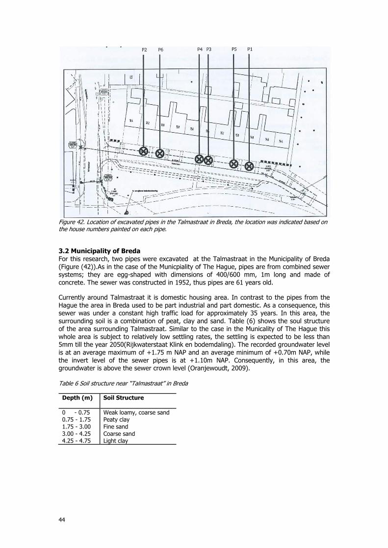
Figure 42. Location of excavated pipes in the Talmastraat in Breda, the location was indicated based on the house numbers painted on each pipe.

3.2 Municipality of Breda

For this research, two pipes were excavated at the Talmastraat in the Municipality of Breda (Figure (42)).As in the case of the Municpiality of The Hague, pipes are from combined sewer systems; they are egg-shaped with dimensions of 400/600 mm, 1m long and made of concrete. The sewer was constructed in 1952, thus pipes are 61 years old.

Currently around Talmastraat it is domestic housing area. In contrast to the pipes from the Hague the area in Breda used to be part industrial and part domestic. As a consequence, this sewer was under a constant high traffic load for approximately 35 years. In this area, the surrounding soil is a combination of peat, clay and sand. Table (6) shows the soul structure of the area surrounding Talmastraat. Similar to the case in the Municality of The Hague this whole area is subject to relatively low settling rates, the settling is expected to be less than 5mm till the year 2050(Rijkwaterstaat Klink en bodemdaling). The recorded groundwater level is at an average maximum of +1.75 m NAP and an average minimum of +0.70m NAP, while the invert level of the sewer pipes is at +1.10m NAP. Consequently, in this area, the groundwater is above the sewer crown level (Oranjewoudt, 2009). Table 6 Soil structure near “Talmastraat” in Breda

Depth (m)

Soil Structure

0 - 0.75 0.75 - 1.75 1.75 - 3.00 3.00 - 4.25 4.25 - 4.75

Weak loamy, coarse sand Peaty clay Fine sand Coarse sand Light clay

45

3.3 New pipe “De Hamer”

The new concrete sewer pipe, from De Hamer factory, is egg-shaped, with dimensions of

400/600 mm was used to validate experimental results (Figure (43)). The new pipe was 2 m

long, being shortened to 0.85 m length to allow testing in the same test facility. The pipe

is made out of concrete and is constructed according to the European quality norm NEN-EN 1916, national additional NEN 7126 and certified according the assessment guidelines BRL 9201.

Figure 43 Display of a new pipe from De Hamer factory.

46

Annex C Dimensions movement measuring device

476 mm

41.12 mm

Top view

Side view

50,18

146,0

147,6

50,11

25,08

39,76

11,28 344

710

11,28

Center of the

39,76

11,28 344

72.50 mm

47

Annex D Article

"Uncertainties associated with laser profiling of concrete sewer pipes for the quantification of the interior geometry."

This article was downloaded by: [Bibliotheek TU Delft]On: 11 August 2014, At: 07:21Publisher: Taylor & FrancisInforma Ltd Registered in England and Wales Registered Number: 1072954 Registered office: Mortimer House,37-41 Mortimer Street, London W1T 3JH, UK

Structure and Infrastructure Engineering:Maintenance, Management, Life-Cycle Design andPerformancePublication details, including instructions for authors and subscription information:http://www.tandfonline.com/loi/nsie20

Uncertainties associated with laser profiling ofconcrete sewer pipes for the quantification of theinterior geometryFrançois Clemensab, Nikola Stanića, Walter Van der Schoota, Jeroen Langeveldac & Mathieu

Lepota

a Water Management Department, Faculty of Civil Engineering and Geosciences, DelftUniversity of Technology, PO Box 5048, 2600 GA, Delft, The Netherlandsb Deltares, PO Box 177, 2600 MH, Delft, The Netherlandsc Royalhaskoning DHV, PO Box 1132, 3800 BC, Amersfoort, The NetherlandsPublished online: 08 Aug 2014.

To cite this article: François Clemens, Nikola Stanić, Walter Van der Schoot, Jeroen Langeveld & Mathieu Lepot(2014): Uncertainties associated with laser profiling of concrete sewer pipes for the quantification of the interiorgeometry, Structure and Infrastructure Engineering: Maintenance, Management, Life-Cycle Design and Performance, DOI:10.1080/15732479.2014.945466

To link to this article: http://dx.doi.org/10.1080/15732479.2014.945466

PLEASE SCROLL DOWN FOR ARTICLE

Taylor & Francis makes every effort to ensure the accuracy of all the information (the “Content”) containedin the publications on our platform. However, Taylor & Francis, our agents, and our licensors make norepresentations or warranties whatsoever as to the accuracy, completeness, or suitability for any purpose of theContent. Any opinions and views expressed in this publication are the opinions and views of the authors, andare not the views of or endorsed by Taylor & Francis. The accuracy of the Content should not be relied upon andshould be independently verified with primary sources of information. Taylor and Francis shall not be liable forany losses, actions, claims, proceedings, demands, costs, expenses, damages, and other liabilities whatsoeveror howsoever caused arising directly or indirectly in connection with, in relation to or arising out of the use ofthe Content.

This article may be used for research, teaching, and private study purposes. Any substantial or systematicreproduction, redistribution, reselling, loan, sub-licensing, systematic supply, or distribution in anyform to anyone is expressly forbidden. Terms & Conditions of access and use can be found at http://www.tandfonline.com/page/terms-and-conditions

Uncertainties associated with laser profiling of concrete sewer pipes for the quantification of theinterior geometry

Franc�ois Clemensa,b*, Nikola Stanica1, Walter Van der Schoota2, Jeroen Langevelda,c3 and Mathieu Lepota4

aWater Management Department, Faculty of Civil Engineering and Geosciences, Delft University of Technology, PO Box 5048, 2600 GADelft, The Netherlands; bDeltares, PO Box 177, 2600 MH Delft, The Netherlands; cRoyalhaskoning DHV, PO Box 1132, 3800 BC

Amersfoort, The Netherlands

(Received 14 March 2014; final version received 14 April 2014; accepted 28 April 2014)

Structural strength and hydraulic capacity are two essential parameters in the assessment of the need for sewer rehabilitation.Especially concrete pipes suffer from loss of wall thickness due to biochemical corrosion and, consequently, a decreasingstructural strength along with an increase of hydraulic roughness. Unfortunately, routinely used visual inspection methodsdo not allow a quantification of the internal pipe geometry which would enable not only detecting but also quantifying theprogress of biochemical corrosion. Advances in laser technology and digital cameras theoretically allow a cost-effectiveapplication of laser profilers to measure the interior geometry of sewer pipes. An analysis of associated uncertaintiesrevealed that the position and alignment of the laser are the main source of measurement errors. A full-scale laboratory set-up demonstrated, based on tests on a new and an 89 years old corroded sewer pipe, that laser scanning is indeed capable ofmeasuring the interior geometry accurately enough to determine wall thickness losses for corroded pipes, provided that theposition and alignment of the laser and camera are accounted for. The obtained accuracy, however, was not enough toquantify the hydraulic roughness.

Keywords: sewer systems; corrosion; inspections; uncertainties; laser profiling

List of symbols

q 2014 Taylor & Francis

Symbol DescriptionDimension/unit

a, b, c Coefficients defining the plane of thereflection board

L21m21

bxCamFRONT x, y coordinates of a point as observedon the optical sensor

Lm

byCamFRONT Sensor of CamFRONT LmbxCamBACK x, y coordinates of a point as observed

on the optical sensorLm

byCamBACK Sensor of CamBACK Lmdi Distance between stationary laser

stand and reflection board for laserdistance meters i ¼ 1,2,3 incoordinate system R(3)

Lm

dz,FRONT Distance between laser sheet and lensplane for CamFRONT

Lm

dz,BACK Distance between laser sheet and lensplane for CamBACK

Lm

ez,FRONT Distance between optical sensor andlens plane for CamFRONT

Lm

ez,BACK Distance between optical sensor andlens plane for CamBACK

Lm

Symbol DescriptionDimension/unit

pCð2Þc2i¼1;2;3

x,y location of the projection of laseri ¼ 1, 2, 3 in the coordinate systemC(2)

Lm

pRð2Þc2i¼1;2;3

x, y location of the projection of laseri ¼ 1, 2, 3 in the coordinate systemR(2)

Lm

pRð2Þ

reference;1!2

Vector between the x and ycoordinates of lasers 1 and 2 in thecoordinate system R(2)

Lm

pRð2Þ

1!2

Vector between the x and ycoordinates of the projected pointsof lasers 1 and 2 in the coordinatesystem R(2)

Lm

Rz ð2Þ Two-dimensional rotation matrix for

the z-axis–/–

Rz ð3Þ Three-dimensional rotation matrix for

the z-axis–/–

RCð2Þ Transformation matrix in coordinate s

ystem C(2)–/–

RCð3Þ Transformation matrix in coordinate

system C(3)–/–

*Corresponding author. Email: f.h.l.r.clemens@tudelft.nl

Structure and Infrastructure Engineering, 2014

http://dx.doi.org/10.1080/15732479.2014.945466

Dow

nloa

ded

by [

Bib

lioth

eek

TU

Del

ft]

at 0

7:22

11

Aug

ust 2

014

1. Introduction

Sewer systems are very capital-intensive infrastructure

systems with a long service life. In many countries around

the world, sewer operators are under pressure to minimise

their maintenance costs, while keeping the risk of failures

at an acceptable level. This requires information on the

current status and the evolution of the status by repeated

measurement of the assets, as well as being able to predict

their future status. The most common method used to

deliver this information on the current status is visual

inspection, closed-circuit television (CCTV). The infor-

mation content of visual inspections, however, is by

definition limited to failures that can be noticed visually.

In addition to that, research (Kirkham, Kearney, Rogers, &

Mashford, 2000) has shown that CCTV inspections are

error prone; recent literature shows that inspectors have a

25% probability to overlook any given defect (Dirksen

et al., 2013). Apart from overlooking defects, there is

crucial information that principally cannot be obtained by

this technique, e.g. loss of wall thickness due to corrosion,

changes in exact position and orientation of a pipe due to

subsidence and information on the hydraulic roughness.

As a consequence, sewer operations experience a lack of

suitable information on the status of the sewers for

adequate sewer asset management (van Riel, Langeveld,

Herder, & Clemens, 2012).

For gravity sewers, three main classes of failures can

be distinguished: water tightness, structural stability and

operational reliability. The latter two are considered to be

the most important failure classes for decisions on sewer

rehabilitation. In order to overcome the limitations of

visual inspection, several new techniques have been

developed over the past two decades and are applied in

practice (Wirahadikusumah, Abraham, Iseley, & Prasanth,

1998), like radar (e.g. Olhoeft, 2000), acoustic techniques

(e.g. Feng, Horoshenkov, Tareq, & Tait, 2012) or sonar

(Kirkham et al., 2000), laser profiling (Duran, Althoefer, &

Seneviratne, 2003) or a combination of these technologies

in order to benefit from the strengths of each technology

(Duran, Althoefer, & Seneviratne, 2007; EPA, 2010).

A recent and comprehensive review of existing techniques

for condition assessment of underground infrastructure,

including sewer systems, can be found in Hao et al. (2012).

Laser profiling of (sewer) pipes is a technology that is

introduced and applied in practice for some years. Main

applications are checks on ovality or other significant

deformations of the geometry and the detection of damages

such as cracks or obstacles (see, e.g. Arsenio, Vreeburg, &

Rietveld, 2013; Duran et al., 2003; Gooch, Clarke, & Ellis,

1996). In addition, the 3D picture that is obtained of the

pipe interior could, provided that the monitoring accuracy

is sufficient, be used to assess the hydraulic roughness of

the pipe (Pegram & Pennington, 1996).

It was shown by Stanic, van der Schoot, Kuijer,

Langeveld, and Clemens (2013) that for corroded sewer

pipes the roughness value, in terms of hydraulic friction

factor (HFF), an accuracy of 3.5% is obtainable. To this

end a Nikon LC60Dx scanner with a resolution in x and y

directions of 7mm and accuracy in z-direction of 60mmwas applied. Based on the general ‘rule of thumb’

(Clemens, 2001) that the monitoring accuracy should be

about 10 times smaller than the time and space scale of the

measured process, the monitoring accuracy should be

0.15mm on a 0.15–0.15mm grid for new pipes with a

typical hydraulic roughness of 1.5 and 2mm on a 2–2mm

grid for heavily corroded pipes with a typical hydraulic

roughness of 20mm.

In addition, some authors also claim that the laser

profiling technique is capable of measuring the wall losses

due to corrosion (Kirkham et al., 2000) with a relative

uncertainty of 0.5%. This implies that in a 600mm circular

sewer, wall losses higher than 3mm could potentially be

measured. Given the typical wall thickness of 80mm for a

600mm concrete sewer, this 3mm seems to be sufficiently

Symbol DescriptionDimension/unit

sFRONT Scaling factor for CamFRONT –/–sBACK Scaling factor for CamBACK –/–V Vector containing all the measured

variables for the uncorrectedprojected points

Various

Vc Vector containing all the measuredvariables for the correctedprojected points

Various

x, y, z Coordinates Lmxi, yi x, y location of laser i ¼ 1, 2, 3 in the

reference coordinate system R(3)Lm

fx Rotation angle around x-axis Angle radfy Rotation angle around y-axis Angle radfz Rotation angle around z-axis Angle radDx x-shift of the camera platform in

R(2,3)Lm

Dy y-shift of the camera platform inR(2,3) LmDz z-shift of the camera platform in R(3) LmDorig Vector containing Dx, Dy and Dz Lmsi Standard deviation in parameter i VariousR(2) Reference coordinate system in two

dimensions (z ¼ 0)–

R(3) Reference coordinate system in threedimensions

–

C(2) Moving platform coordinate systemin two dimensions (z ¼ 0)

–

C(3) Moving platform coordinate systemin three dimensions

–

o, r, n Three vectors define the orthogonalbase for the coordinate system C(3)

Lm

on, rn, nn Normalised orthogonal basis for thecoordinate system C(3)

–/–

F. Clemens et al.2

Dow

nloa

ded

by [

Bib

lioth

eek

TU

Del

ft]

at 0

7:22

11

Aug

ust 2

014

accurate as input for the purpose of assessing the

constructional strength and stability.

However, amongst others, Duran et al. (2003) state that

the main difficulty in laser profiling is the alignment and

orientation of the sensor in the harsh sewer environment.

Even small misalignments and shift in position can cause a

significant systematic error in the measured internal

geometry (Stanic et al., 2013; van der Schoot, 2014).

In current practice, uncertainties due to unknown misalign-

ments remain unnoticed, rendering the laser profiling

technique without correction of the alignment and position

unsuitable for measuring the exact internal geometry.

In this article, the uncertainties associated with the

application of laser profiling in order to obtain a 3D profile

of corroded concrete (sewer) pipes are analysed. The

uncertainty analysis revealed the significance of the

different sources of errors in the laser profiler monitoring

results. Based on this, an improvement of the available

laser profilers is proposed and tested in a full scale pilot

using a corroded egg-shaped concrete sewer pipe and one

new egg-shaped pipe that has not been in service. Based on

laboratory experiments and theoretical analysis, future

developments are defined.

2. Laser profiling: measuring uncertainties

Laser profiling of sewer pipes is based on a combination of

projecting rings of light on the sewer pipe wall and

capturing the images by a digital camera. Laser profilers

are commonly placed on top of a CCTV camera tractor in

order to be able to move them through the sewer pipe, as

shown in Figure 1.

The accuracy of the results obtained by laser profiling

is determined by: (1) the quality of the camera, i.e. the

number of pixels, the pixel size and the number of frames

per second that can be recorded, (2) the quality of the

circular laser projection, which determines the width of the

projected rings of light, (3) the method used to determine

the position of the camera during its movement through

the sewer, which determines the position of each recorded

frame and consequently the distance between the frames

and (4) the alignment of the laser and camera, which

determine the angle of the projection and consequently the

extent of deformation of the projection.

The impact of the quality of the camera and lasers on

the uncertainties can be assessed by checking the

specifications of the equipment by practical tests. The

position of the camera and laser is normally determined by

measuring the rotation of the wheels of the camera tractor

or of the cable that is used to pull the camera tractor

through the sewer. As the wheels of the camera tractor are

likely to skid in the sewer, the position of the laser and

camera can be rather imprecise (Dirksen, Pothof,

Langeveld, & Clemens, 2014). Another bias could be

introduced by the use of the cable to estimate distance: the

cable follows the path of the tractor (not necessarely

parallel to the pipe) and the flexion of the cable. Moreover,

the alignment of the camera and laser is normally not

accounted for. As a consequence, this adds to the unknown

bias related to the position.

3. Material and methods

3.1. Measuring set-up

To assess the uncertainties associated with laser profiling,

the measuring set-up shown in Figure 2 has been designed

with all the monitoring equipment placed on a mobile

platform. The set-up consists, like for ordinary laser

profilers, of a laser projector combined with a camera,

referred to as camFRONT. The laser uses a reflecting cone to

produce a laser sheet which projects a line perpendicular to

the main axis of the platform on the inner pipe wall. The

mobile platform moves at a, not necessarily constant,

speed of approximately 0.05m/s through the pipe, the

recording frequency of camFRONT is 30 frames/s, implying

that each frame is about 1.7mm apart along the length of

the pipe. The images recorded by camFRONT are stored on

a measuring computer for further processing.

Accurately measuring the position and alignment of

the camera and laser requires that information is available

on the x, y and z positions and rotation around these axes.

In the experiments, this information is obtained by using a

set-up comprising three parallel lasers with a fixed

position, each measuring the distance between the parallel

lasers and a reflection board. A second camera, referred to

as camBACK, records the position of the three points

projected by the parallel lasers on the reflection board. The

frame rate of camBACK is 8 frames/s, implying that every

6.25mm there is a recording of the distance between

reflection board and the three lasers.

Figure 1. Photograph of the experimental set-up.

Structure and Infrastructure Engineering 3

Dow

nloa

ded

by [

Bib

lioth

eek

TU

Del

ft]

at 0

7:22

11

Aug

ust 2

014

The three parallel lasers have a fixed position and

define a reference coordinate system, with the z-axis being

parallel to the main axis of the pipe. A left-handed

coordinate system is applied, while the rotation angles are

defined in the Tait-Bryan formalism (Figure 3), see e.g.

Baranowski (2013). The images recorded by camBACK and

the readings from the laser distance meters are stored on

the same measuring computer as camFRONT.

For each frame recorded by the front camera, the exact

position and orientation of this camera should be known;

therefore, for each frame, the position of the three laser

points projected on the reflection board has to be known.

It is important that the synchrony of the images recorded

with the front camera and the back camera is guaranteed.

Synchrony is guaranteed by the fact that both cameras

were connected to the same data-acquisition system,

which enforced both data sources into the same time base.

3.1.1. Accuracy of camera sensors

The measuring error of the 2D projection of the wall of the

pipe is calculated using the average number of pixels that

are illuminated on the sensor of camFRONT, depending on

the scale factor, defined by the ratio between the distance

between the laser sheet and the lens and the distance

between the lens and sensor plane. The sensor used in

camFRONT is a 2/300 sensor with 1024 £ 760 pixels, pixel

dimensions are 6.45mm £ 6.45mm. Based on an analysis

of 20 repetitive samples in 20 different video frames, in

which the measuring system was stationary, all rotation

angles were equal to zero and the camera positioned in the

axis of the conduit revealed that the laser sheet illuminated

about 9–10 pixels. Figure 4 shows the results of the

distribution of the recorded light intensity across the

projected line on the camera sensor. Based on these

experiments, the standard deviation in the position was

estimated to be sx,y,camFRONT ¼ 13mm.

CamBACK is used to keep track of the position of the

three points projected on the reflection board by the three

stationary lasers. The obtained image of these points is

transferred into contour lines using standard image

processing routines. On these contour lines, an ellipse is

fitted from which the intersection point of both axes

defined as the x and y location of the point (in sensor

Figure 2. Sketch of the experimental set-up, details on the dimensions and materials used can be found in Tables 1 and 2.

Figure 3. Left-handed coordinate system and definition of theTait-Bryan angles.

Table 1. Specifications and their standard uncertainties(obtained by repeated measurement) of the instrumentation.

Brand/modelStandard uncertainty

s

camFRONT and thetractor

Panoramo/3DopticalPipeline scanner

13mm

camBACK D link/DCS 2310 L 5.6mmLaser distance meters Fluke/414D 0.5mmCircular projectedlaser

Ibak/ILP –

Dimensions of themeasuring set-up

– 0.25mm

Table 2. Dimensions of the measuring set-up.

Measure Value (m)

dzcamFRONT 0.4760dzcamBACK 0.3540ezcamFRONT 0.003440ezcamBACK 0.002860camoffx 0.0020 (0.0022)camoffy 20.2307 (20.2248)camoffz 0.1647 (0.16466)

Note: The figures between brackets for the camera offset values are validfor the old pipe, and the other values are valid for the new pipe.

F. Clemens et al.4

Dow

nloa

ded

by [

Bib

lioth

eek

TU

Del

ft]

at 0

7:22

11

Aug

ust 2

014

coordinates) is derived. Analysing 30 independent frames

resulted in a standard deviation in both x and y directions

of about 2 pixels. The sensor of camBACK is a 1/400 sensorwith a resolution of 1280 £ 800 pixels with a pixel width

of 2.8mm £ 2.8mm, resulting in estimated standard

deviation of sx,y,camBACK ¼ 5.6mm. The cameras were

tested on lens distortion effects (e.g. barrel distortion), for

camFRONT these proved to be not observable, for

camBACK there was some distortion at the far corners of

the image. During the experiments, care was taken to

avoid that the laser dots were recorded in these (slightly)

distorted areas.

3.1.2. Accuracy of laser alignment

The alignment of the lasers was determined by repeated

measurement of the distance between the three projected

points at a distance of 30m, the maximum mutual

deviation over this distance between the projected points

was ^3mm (95% confidence interval in 30 repeated

measurements) when compared with their position at the

origin. This implies that the standard deviation of the

alignment was estimated to be 2.5 £ 1025 radials.

Figure 4. Distribution of the light intensity on the sensor of camFRONT.

Figure 5. Definition sketch coordinate systems.

Structure and Infrastructure Engineering 5

Dow

nloa

ded

by [

Bib

lioth

eek

TU

Del

ft]

at 0

7:22

11

Aug

ust 2

014

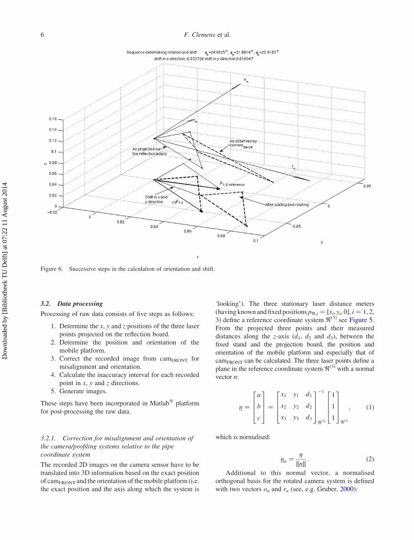
3.2. Data processing

Processing of raw data consists of five steps as follows:

1. Determine the x, y and z positions of the three laser

points projected on the reflection board.

2. Determine the position and orientation of the

mobile platform.

3. Correct the recorded image from camFRONT for

misalignment and orientation.

4. Calculate the inaccuracy interval for each recorded

point in x, y and z directions.

5. Generate images.

These steps have been incorporated in Matlabw platform

for post-processing the raw data.

3.2.1. Correction for misalignment and orientation of

the camera/profiling systems relative to the pipe

coordinate system

The recorded 2D images on the camera sensor have to be

translated into 3D information based on the exact position

of camFRONT and the orientation of themobile platform (i.e.

the exact position and the axis along which the system is

‘looking’). The three stationary laser distance meters

(having known and fixed positions pR,i ¼ [xi, yi, 0], i ¼ 1, 2,

3) define a reference coordinate system R(3) see Figure 5.

From the projected three points and their measured

distances along the z-axis (d1, d2 and d3), between the

fixed stand and the projection board, the position and

orientation of the mobile platform and especially that of

camFRONT can be calculated. The three laser points define a

plane in the reference coordinate system R(3) with a normal

vector n:

n ¼a

b

c

26643775 ¼

x1 y1 d1

x2 y2 d2

x3 y3 d3

2664

377521

Rð3Þ

1

1

1

26643775Rð3Þ

; ð1Þ

which is normalised:

nn ¼n

nk k : ð2ÞAdditional to this normal vector, a normalised

orthogonal basis for the rotated camera system is defined

with two vectors on and rn (see, e.g. Gruber, 2000):

Figure 6. Successive steps in the calculation of orientation and shift.

F. Clemens et al.6

Dow

nloa

ded

by [

Bib

lioth

eek

TU

Del

ft]

at 0

7:22

11

Aug

ust 2

014

Figure 7. Difference between theoretical and measured geometry for the new pipe. The upper chart shows the uncorrected result, and thelower chart shows the result after correction for position and orientation of the measuring platform.

Figure 8. Difference between theoretical and measured geometry for the old pipe. The upper chart shows the uncorrected result, and thelower chart shows the result after correction for position and orientation of the measuring platform.

Structure and Infrastructure Engineering 7

Dow

nloa

ded

by [

Bib

lioth

eek

TU

Del

ft]

at 0

7:22

11

Aug

ust 2

014

o ¼ j2 ð j�nnÞ £ nn

j ¼ 0 1 0� �

r ¼ o £ nn

on ¼ o

ok krn ¼ r

rk k

9>>>>>>>>>>=>>>>>>>>>>;: ð3Þ

These three vectors define a transformation matrix (RCð3Þ )

for the camera space C(3):

RCð3Þ ¼

rnð1Þ onð1Þ nnð1Þrnð2Þ onð2Þ nnð2Þrnð3Þ onð3Þ nnð3Þ

2664

3775: ð4Þ

Since the projection on the reflection board is in a plane,

the transformation of the position of the laser points as

recorded by camBACK to the x y plane in R(2)

(transformation C(2) ! R(2)) uses the following trans-

formation matrix (RCð2Þ ):

Figure 9. Definition sketch for the angles indicated in Figures10–17, 08 is the invert level going counterclockwise the crown isat 1808.

Figure 10. Difference between corrected and uncorrected profiles for one frame obtained from the new pipe.

F. Clemens et al.8

Dow

nloa

ded

by [

Bib

lioth

eek

TU

Del

ft]

at 0

7:22

11

Aug

ust 2

014

Figure 11. Standard deviation for the new pipe for one frame using smisalignment ¼ 2.5 £ 1025 radials.

RCð2Þ ¼

rnð1Þ onð1Þrnð2Þ onð2Þ

" #: ð5Þ

Using this matrix, coordinate transformations between

spaces R(2) and C(2) for a point pc BACK ¼ [bx BACK,

byBACK] as recorded on the sensor of camBACK can bemade,

taking into account the scaling factor (sBACK) of camBACK5:

sBACK ¼ dzBACK

ezBACKð6Þ

and

pRð2Þ ¼ sBACKRCð2ÞpcBACK: ð7Þ

Note that this is a non-orthogonal transformation, i.e.

angles and distances are not conserved. This is due to the

fact that the laser beams are stationary and the reflection

board is shifted and rotated. As a consequence, a

deformation (stretch) of the original positions of the

projected points occurs. Therefore, prior to rotation, the

shift and scale should be applied. As a first step, it is

necessary to do a coordinate transform from the projected

points in the coordinate system C(2) to the reference

coordinate system R(2):

pRð2Þi¼1;2;3

¼ sBACKRCð2ÞpcBACKi¼1;2;3: ð8Þ

Subsequently, the projected points are corrected for the

shift in x, y and z directions. The correction in the z-

direction is equal to 1/c (being the distance between the

reference stand and the reflection board), the shift in x and

y directions are made based on the coordinates of the

origin6 (x1, y1)R(2) ¼ (0, 0)R

(2):7

Dx

Dy

" #Rð2Þ

¼ Dð2Þorig ¼ pRð2Þ

1;

ðTÞpRð2Þi¼1;2;3

¼ pRð2Þi¼1;2;3

2 pRð2Þ1:

ð9Þ

At this stage, the points are defined in the z ¼ 0 plane of

the reference coordinate system R(2), not corrected for the

rotation around the z-axis however. Two points (e.g. ðTÞpRð2Þ1

and ðTÞpRð2Þ2, or any other combination of two points) define

a vector ðTÞpRð2Þ1!2

that can be used to define the rotation

around the z-axis:

Structure and Infrastructure Engineering 9

Dow

nloa

ded

by [

Bib

lioth

eek

TU

Del

ft]

at 0

7:22

11

Aug

ust 2

014

uz ¼ sign pRð2Þreference;2

ð1Þ2ðTÞ pRð2Þ2ð1Þ

h i

arccos

pRð2Þ

reference;1!2

�ðTÞpRð2Þ1!2

pRð2Þ

reference;1!2

�������� ðTÞpRð2Þ

1!2

��� ���

2664

3775: ð10Þ

The first term determines the direction of rotation

(counterclockwise is positive). The next step is to rotate

ðTÞpRð2Þi¼1;2;3

with 2uz:

pRð2Þi¼1;2;3

¼ Rz ð2ÞðTÞpRð2Þ

i¼1;2;3; ð11Þ

with

Rz ð2Þ ¼

cosð2uzÞ sinð2uzÞ2sinð2uzÞ cosð2uzÞ

" #

¼cosðuzÞ 2sinðuzÞsinðuzÞ cosðuzÞ

" #: ð12Þ

Figure 6 presents an example of the successive

operations defined in Equations (1)–(12). At this point,

the orientation for x, y and z axes as well as the shift of the

positions x, y and zof themoving camera platform is known,

allowing the position of camFRONT to be determined:

xCamFRONT

yCamFRONT

zCamFRONT

26664

37775

Rð3Þ

¼RCð3ÞRz ð3Þ

xoffset;CamFRONT

yoffset;CamFRONT

zoffset;CamFRONT

26664

37775

Cð3Þ

þ

Dð2Þorigð1Þ

Dð2Þorigð2Þc21

266664

377775;

ð13Þ

with

Rz ð3Þ ¼

cosðuzÞ sinðuzÞ 0

2sinðuzÞ cosðuzÞ 0

0 0 1

2664

3775: ð14Þ

The first term in Equation (13) is the rotation of the

camera relative to the origin followed by the shift of the

origin along the x-, y- and z-axis of the reference

Figure 12. Standard deviation for the new pipe for one frame using smisalignment ¼ 8.3 £ 1026 radials.

F. Clemens et al.10

Dow

nloa

ded

by [

Bib

lioth

eek

TU

Del

ft]

at 0

7:22

11

Aug

ust 2

014

coordinate system. Finally, an observed point (reflection

from the pipe wall) pc1 ¼ [bx1, by1] on the sensor of

camFRONT with camera coordinates [bx,1, by,1] translates

into the (corrected) x, y and z positions in the reference

coordinate system R(3):

with cosðuxÞ ¼ffiffiffiffiffiffiffiffiffiffia 2þc 2

pffiffiffiffiffiffiffiffiffiffiffiffiffiffiffiffia 2þb 2þc 2

ph i

cosðuyÞ ¼ cffiffiffiffiffiffiffiffiffiffia 2þc 2

ph i

; ð16Þand

sCamFRONT ¼ dzCamFRONT

ezCamFRONT

ð17Þ

pRð3Þcorrected

¼ RCð3ÞRz ð3Þ

sCamFRONTbx1

sCamFRONTby1

0

2664

3775þ

xCamFRONT

yCamFRONT

zCamFRONT

2664

3775Rð3Þ

þ0

0

cosðuxÞcosðuyÞdzCamFRONT

2664

3775

¼ RCð3ÞRz ð3Þ

sCamFRONTbx1

sCamFRONTby1

0

2664

3775þ R

Cð3ÞRz ð3Þ

xoffset;CamFRONT

yoffset;CamFRONT

zoffset;CamFRONT

2664

3775Cð3Þ

þDð2Þorigð1Þ

Dð2Þorigð2Þc21

26664

37775þ

0

0

cosðuxÞcosðuyÞdzCamFRONT

2664

3775

¼ RCð3ÞRz ð3Þ

sCamFRONTbx1

sCamFRONTby1

0

2664

3775þ R

Cð3ÞRz ð3Þ

xoffset;CamFRONT

yoffset;CamFRONT

zoffset;CamFRONT

2664

3775Cð3Þ

þDð2Þorigð1Þ

Dð2Þorigð2Þ

c21 þ dzCamFRONTc=ffiffiffiffiffiffiffiffiffiffiffiffiffiffiffiffiffiffiffiffiffiffiffiffiffiffia2 þ b2 þ c2

p

26664

37775

9>>>>>>>>>>>>>>>>>>>>>>>>>=>>>>>>>>>>>>>>>>>>>>>>>>>;

; ð15Þ

Figure 13. Standard deviation for the new pipe for one frame for the uncorrected profile.

Structure and Infrastructure Engineering 11

Dow

nloa

ded

by [

Bib

lioth

eek

TU

Del

ft]

at 0

7:22

11

Aug

ust 2

014

denotes the scaling factor for camFRONT.

The term dzCamFRONTc=ffiffiffiffiffiffiffiffiffiffiffiffiffiffiffiffiffiffiffiffiffiffiffiffiffiffia2 þ b2 þ c 2

pin Equation

(15) is the projection of the distance between camFRONT

and the laser sheet on the z-axis in the reference coordinate

system R(3).

3.2.2. Uncertainties analysis

The overall uncertainty of the position of a point projected

on the pipe wall is determined as follows:

. The uncertainty of the recorded images in camFRONT

and camBACK.. The uncertainty of the measured distances d1,2,3.. The uncertainty of the alignment of the lasers.. The uncertainty of the fixed distances in the

measuring set-up.

Assuming that the measuring uncertainties in the

parameters mentioned are mutually independent, hence

neglecting covariance terms, the law of propagation of

uncertainties (JCGM 104, 2009) applies for the measured

points:

s2pcorrected

¼Xi¼19

i¼1

s2vcðiÞ

›pcorrected›vcðiÞ

� �2; ð18Þ

in which

The uncertainty of the uncorrected point is calculated

in the same manner:

s2p ¼

Xi¼8

i¼1

s2vi

›p

›vi

� �2; ð20Þ

with

v ¼ di¼1;2;3; bx1; by1; dzFRONT; ezFRONT;amisal

� �; ð21Þ

Figure 14. Difference between corrected and uncorrected profiles for one frame obtained from the old pipe.

vc ¼di¼1;2;3; xi¼1;2;3; yi¼1;2;3; bx1; by1; bx2; by2;

xoffsetcamFRONT;BACK; yoffsetcamFRONT;BACK; zoffsetcamFRONT;BACK; dzFRONT; dzBACK; ezFRONT; ezBACK;amisal

!: ð19Þ

F. Clemens et al.12

Dow

nloa

ded

by [

Bib

lioth

eek

TU

Del

ft]

at 0

7:22

11

Aug

ust 2

014

where amisal is the misalignment of the lasers. Due to the

very complicated analytical expressions that would result

for most of the terms in Equations (18) and (20), the

quantification has been done numerically using partial

differences estimates.

4. Experimental results

Two concrete sewer pipes were subjected to the analysis as

described before, one new egg-shaped pipe with an inner

nominal geometry of 400/600mm8 and one egg-shaped

pipe (400/600mm) that was in service for more than 89

years in the municipality of the Hague, showing clear

marks of crown corrosion and concretions of sediments at

the sides.

Figure 7 depicts the results for the new pipe. The charts

indicate the difference between the profiles measured

following the procedures as described before minus the

theoretical profile. In the upper chart, the result is shown

without correcting for position and orientation of the

mobile platform, while in the lower chart, the correction

has been applied. As can be seen, the differences between

measurement and theoretical profiles are, overall, much

smaller for the corrected measurements. It is also noted

that both corrected and uncorrected measurements deviate

from the theoretical profile with a few millimetres,

probably this is due to the allowed tolerance in the

production process (see, e.g. Clemens, 2001).

This can also be observed in Figure 8 for the 89 years

old egg-shaped pipe. Without correction there are

significant differences (loss of wall thickness) at the

invert of the pipe, which was not visually observed, while

the effect of crown corrosion is exaggerated to have a

maximum value of 20mm. After correction (lower chart in

Figure 8), there is no loss of wall thickness at the invert

while this reaches a maximum of 15mm at the top due to

crown corrosion. It is also noticeable that a large area at

the crown shows significant less loss of wall thickness

after correction. It is also observed that at 200mm along

the perimeter of the pipe, along the length a difference of

about 210mm occurs, which is shifted to the right along

the perimeter in the uncorrected measurement, while in the

corrected measurements, this band is more or less parallel

to the axis of the pipe.

Figure 15. Standard deviation for the old pipe for one frame using smisalignment ¼ 2.5 £ 1025 radials.

Structure and Infrastructure Engineering 13

Dow

nloa

ded

by [

Bib

lioth

eek

TU

Del

ft]

at 0

7:22

11

Aug

ust 2

014

Figure 10 (definition sketch is shown in Figure 9)

illustrates the difference between the uncorrected and

corrected profiles for one typical frame obtained from the

measurements on the new pipe, while Figures 11 and 12

show sx, sy and sz as a function of the perimeter for

smisaligment ¼ 2.5 £ 1025 radials (Figure 11) and

smisaligment ¼ 8.3 £ 1026 radials (Figure 12).

smisaligment ¼ 2.5 £ 1025 is the standard deviation deter-

mined for the alignment of the lasers (see Section 3.1.2),

the value of 8.3 £ 1026 radials, being one-third of this

value, is used to illustrate the sensitivity of the accuracy for

the misalignment.

Figure 13 shows sx, sy andsz for the uncorrected profile

of the same frame. Figures 14–17 show the same

information for a typical frame as obtained from the old

pipe. As can be seen, the difference between corrected and

uncorrected profiles as well as the accuracy of the

measurements varies along the perimeter of the profile and

is strongly influenced by the accuracy of the alignment of the

lasers. Figures 18 and 19 present two typical examples of the

relative contributions to the measuring uncertainty of the

different sources for smisaligment ¼ 2.5 £ 1025 radials and

smisaligment ¼ 8.3 £ 1026 radials, respectively, for the new

pipe. As can be seen, the misalignment is dominant when

smisaligment ¼ 2.5 £ 1025 radials (60–90% of the uncer-

tainty is caused by this factor, while this drops to 15–50%

when smisaligment ¼ 8.3 £ 1026 radials). A similar obser-

vation is made for the results for the old pipe shown in

Figures 20 and 21.

Tables 3 and 4 summarise the results. A one-sided t-

test with acceptance level p ¼ 0.95 shows that for the new

pipe only the differences in the z-direction between

corrected and uncorrected profiles are significant, even if

the alignment of the lasers is improved by a factor of three.

For the old pipe, the observed differences are significant,

with the exception of the z-direction. The results show

clearly that results obtained from laser profiling have a

tendency to overestimate loss of wall thickness if they are

not corrected for position and orientation of the measuring

set-up relative to the pipe. Underestimation will not occur,

since any deviation of a projection perpendicular to the

axis of the pipe will result in an increase in dimension of

the profile recorded.

As an example, the observed differences between

corrected measured and theoretical profiles for the new

pipe at z ¼ 23mm are shown in Figure 22. As can be seen,

Figure 16. Standard deviation for the old pipe for one frame using smisalignment ¼ 8.3 £ 1026 radials.

F. Clemens et al.14

Dow

nloa

ded

by [

Bib

lioth

eek

TU

Del

ft]

at 0

7:22

11

Aug

ust 2

014

a difference between measured corrected and theoretical

profiles is visible (though well within the 95% confidence

interval). Figure 23 displays the difference between

measured corrected and theoretical profiles for the old

pipe at z ¼ 300mm. At the crown, there is a loss of wall

thickness up to 10–14mm, while at the bottom there is a

difference of about 0–6mm.

Figures 24 and 25 present for the old and new pipe,

respectively, the difference between uncorrected and

theoretical profiles. As can be seen, the systematic

differences are significant in both cases. For the old

pipe, it is noticed that the maximum loss of wall thickness

is larger in the uncorrected profile (18mm) than in the

corrected profile (14mm). These figures only serve as an

example. The 95% confidence interval in Figures 22, 23,

24 and 25 is based on the standard uncertainty in the x and

y directions: sloss of wall thickness ¼ffiffiffiffiffiffiffiffiffiffiffiffiffiffiffiffis2x þ s2

y

q, assuming

that the uncertainties in the x and y directions are mutually

independent. It has to be mentioned that this is the

lower limit for sloss of wall thickness, when assuming a

correlation of 1, the upper bound is defined as:

sloss of wall thickness ¼ sx þ sy.

5. Discussion of the results

Using laser-profiling techniques it is possible to obtain

information on the 3D geometry of a pipe. The obtainable

uncertainty in the result is quantified and depends largely

on the uncertainty of the laser distance measurements and

the alignment of the reference coordinate system defined

by three parallel lasers. Using relatively simple instru-

ments, statistically significant differences between cor-

rected and uncorrected profiles in the x, y and z directions

are obtained under laboratory circumstances. It has to be

noted that the covered lengths in the experiments were

relatively small, 17 and 55 cm for the new and old pipe,

respectively. This results in relatively small values for

shifts in the x and y directions. It is anticipated that, when

longer stretches are measured, these shifts will be

significantly higher, resulting in larger systematic

differences between corrected and uncorrected profiles.

It has been shown that, using the corrections as

described in this article, compensation for systematic

errors due to orientation and position of the measuring

platform is possible but at a price of an increased 95%

confidence interval compared to uncorrected measure-

Figure 17. Standard deviation for the old pipe for one frame for the uncorrected profile.

Structure and Infrastructure Engineering 15

Dow

nloa

ded

by [

Bib

lioth

eek

TU

Del

ft]

at 0

7:22

11

Aug

ust 2

014

ments. In the simple set-up and the example shown, the

corrections are not significant for the whole range of

measurements performed. In the laboratory experiments,

relatively simple and cheap instruments (as applied in

practice) are used in order to investigate the practically

feasible uncertainty. It is stressed that, when using high-

end instrumentation, a far better accuracy is obtainable.

The challenge, however, is to develop a measuring system

that is applicable under practical circumstances and

therefore has to be robust and economically feasible.

To this end, the main issues to work on are a more accurate

distance measurement (see, e.g. Minoshima &Matsumoto,

2000) and the exact alignment of the three parallel lasers,

or the implementation of another manner to measure the

orientation and position of camFRONT.

As it has been shown, there are three main contributing

sources of uncertainties, given in descending order: the

misalignment of the lasers, the image quality of the two

cameras and the distance measurement. In laboratory

circumstances, the alignment of the lasers is feasible to

within 2.5 £ 1025 radials. For obtaining a system that is

also applicable in practice, especially this issue seems to

be quite a challenge and subject to further development.

It is anticipated that for practical applications, the

measurement of the orientation of the camera might be

done using optical gyroscopes, although their main

disadvantage is still their high costs.

Typically the price of optical gyroscopes is 10 times

higher than the price of laser distance meters. In the

measuring set-up as presented here, the achievable

accuracy in the orientation of the measuring platform is

in the order of magnitude of 7 £ 1024 radials. Optical

gyroscopes achieve an accuracy in angle measurement in

the order of magnitude of 1027 radials (see, e.g. Titterton

& Weston, 2004). Applying such a device will result in an

overall uncertainty (95% confidence interval) of ^3–

4mm, the accuracy given by Kirkham et al. (2000) while

neglecting misalingment and positioning issues. Apart

from realising a decrease in uncertainty, application of

optical gyroscopes also allows for application in pipes that

have bends; using the set-up as presented in this article the

measuring device must be visible for stationary lasers.

Figure 18. Relative contribution of the individual source of error to the overall measuring error in x, y and z positions for the new pipewith smisalignment ¼ 2.5 £ 1025 radials.

F. Clemens et al.16

Dow

nloa

ded

by [

Bib

lioth

eek

TU

Del

ft]

at 0

7:22

11

Aug

ust 2

014

Application of more accurate and sensitive video

equipment is relatively simple to achieve given the rapid

development of affordable video equipment. It is,

however, questionable whether a more accurate camera

is the key issue here, since the scatter in the light intensity

on the sensor is also determined by the diffusion of the

reflected laser light from the pipe wall, which cannot be

totally controlled. Certainly, the sensor area and the

dimensions of the pixels become more important when

working with large sewer profiles. Possibly the application

of laser light with a shorter wavelength (here a red laser

with a wavelength range of 635–670 nm was applied) will

result in an increase of accuracy since the divergence of a

laser beam is less at shorter wavelengths (see, e.g. Wright,

Greve, Fleischer, & Austin, 1992).

A disadvantage of the presented set-up is that, when

sewers show significant curves, the three laser points may

be projected outside the area of the reflection board.

In such a case, the method will not work, unless the

specific circumstances allow for the stationary lasers to be

moved into the sewer. In such a case, a piece-wise

approach is possible. For very big sewers, the dimensions

of the set-up have to be adapted. For instance, the distance

between the front camera and the laser profiler and the

field of view of the front camera should be such that the

laser projection on the pipe wall is completely visible.

Furthermore, in order to achieve the accuracy sought for,

the mutual distance between the three stationary lasers

should be as large as possible.

Apart from obtaining the 3D inner geometry of a pipe

using the proposed technique, it has been suggested by

Duran et al. (2007) that using pattern recognition, defects

such as cracks, surface damage, intrusion of house and

gully pot connections can be detected. Using these

techniques in combination with the technique presented in

this article, it may become feasible to obtain an efficient

method to collect data on the condition of pipes using just

one apparatus.

6. Conclusions

The interior geometry of sewer pipes and the hydraulic

roughness are sewer properties that drive sewer rehabilita-

Figure 19. Relative contribution of the individual source of error to the overall measuring error in x, y and z positions for the new pipewith smisalignment ¼ 8.3 £ 1026 radials.

Structure and Infrastructure Engineering 17

Dow

nloa

ded

by [

Bib

lioth

eek

TU

Del

ft]

at 0

7:22

11

Aug

ust 2

014

tion to a large extent. Laser profiling has been shown to

potentially be a technique that allows to measure the

interior geometry accurately enough to be able to quantify

the interior geometry and to quantify the hydraulic

roughness for heavily deteriorated pipes, provided that the

position and alignment of the camera and laser are

adequately accounted for. Laser profiler results that are not

corrected are subject to unknown, and potentially very

large, errors, which systematically overestimate wall

losses.

The accuracy of the experimental set-up is mainly

determined by the uncertainty of the distance measure-

ment and the alignment of the three lasers used to quantify

the position and orientation of the camera and the laser

sheet. Applying more accurate laser distance-measuring

techniques easily solves the former; the latter is, certainly

in practical circumstances, a challenge. Improving the

alignment of these lasers, or introducing another method

for measuring the orientation of the mobile platform

allows for an accuracy level leading to an anticipated 95%

confidence interval of about 4–5mm in profiles up to

600mm in dimension, yielding significant differences

between corrected and uncorrected profiles.

Once the 3D geometry is obtained, this can serve as

an input for FEM analysis on the structural strength and

stability (see e.g. de Borst, Crisfield, Remmers, &

Verhoosel, 2012). Certainly, the external profile and

material properties have to be known for this, in most

cases, however, the former can be obtained either from

documentation of the manufacturer, whereas the

material properties can be determined from analysis

of drill cores. Future developments will focus on the

following:

. Alternative methods, e.g. optical gyroscopes, for

determining the orientation.. More accurate laser distance meters.. Construction of a low-cost device that can operate in

practical applications.. Effects on the overall uncertainty using lasers with

smaller wavelengths.. Optimisation of the post-processing software.

Figure 20. Relative contribution of the individual source of error to the overall measuring error in x, y and z positions for the old pipewith smisalignment ¼ 2.5 £ 1025 radials.

F. Clemens et al.18

Dow

nloa

ded

by [

Bib

lioth

eek

TU

Del

ft]

at 0

7:22

11

Aug

ust 2

014

Figure 21. Relative contribution of the individual source of error to the overall measuring error in x, y and z positions for the old pipewith smisalignment ¼ 8.3 £ 1026 radials.

Table 4. Maximum deviation between corrected and uncorrected profiles and the maximum standard deviation for the old pipe.

Maximumdeviation(mm)

Maximum s for the corrected profile (mm)with smisaligment ¼ 2.5 3 1025 radials

Maximum s for the corrected profile (mm)with smisaligment ¼ 8.3 3 1026 radials

s for theuncorrected profile

(mm)

X 15.9 8.9 ( p ¼ 0.96)* 3.7 ( p ¼ 1.00)* 1.8Y 12.8 7.0 ( p ¼ 0.96)* 3.2 ( p ¼ 1.00)* 1.8Z 1.2 4.1 ( p ¼ 0.60) 2.3 ( p ¼ 0.66) 1.5

Notes: Results marked with an asterisk show a significant difference between corrected and uncorrected results for which a one-sided t-test with acceptancelevel p ¼ 0.95 was used. The figures between brackets show the t-test significance level.

Table 3. Maximum deviation between corrected and uncorrected profiles and the maximum standard deviation for the new pipe.

Maximumdeviation(in mm)

Maximum s for the corrected profile withsmisaligment ¼ 2.5 3 1025 radials (in mm)

Maximum s for the corrected profile withsmisaligment ¼ 8.3 3 1026 radials (in mm)

s for theuncorrected profile

(in mm)

X 4.9 6.4 (0.78) 3.2 (0.94) 1.8Y 7.7 14.3 (0.70) 5.7 (0.88) 1.8Z 10.0 4.9 (0.97)* 3.2 (0.99)* 1.5

Notes: Results marked with an asterisk show a significant difference between corrected and uncorrected results for which a one-sided t-test with acceptancelevel p ¼ 0.95 was used. The figures between brackets show the t-test significance level.

Structure and Infrastructure Engineering 19

Dow

nloa

ded

by [

Bib

lioth

eek

TU

Del

ft]

at 0

7:22

11

Aug

ust 2

014

Figure 22. Difference between corrected measured and theoretical profiles for the new pipe.

Figure 23. Difference between corrected measured and theoretical profiles for the old pipe.

F. Clemens et al.20

Dow

nloa

ded

by [

Bib

lioth

eek

TU

Del

ft]

at 0

7:22

11

Aug

ust 2

014

Figure 24. Difference between theoretical and uncorrected profiles for the new pipe.

Figure 25. Difference between uncorrected and theoretical profiles for the old pipe.

Structure and Infrastructure Engineering 21

Dow

nloa

ded

by [

Bib

lioth

eek

TU

Del

ft]

at 0

7:22

11

Aug

ust 2

014

Acknowledgements

The authors specially thank the staff of Van der Valk and deGroot for their assistance with the experimental set-up and forgiving access to their facilities.

Funding

The authors like to acknowledge the funding by (in alphabeticalorder): ARCADIS, Deltares, Royal Haskoning DHV, munici-palities of Almere, Breda, ‘s-Gravenhage, Rotterdam andUtrecht, GMB Rioleringstechnieken, Grontmij, KWR Water-cycle Research Institute, PlatformWater Vallei & Eem, StichtingRIONED, STOWA, Tauw, Van der Valk and de Groot,Waterboard De Dommel, Waternet and Witteveen þ Bos asparticipants of the Urban Drainage Research programme.

Notes

1. Email: n.stanic@tudelft.nl2. Email: waltervanderschoot@gmb.eu3. Email: j.g.langeveld@tudelft.nl4. Email: m.J.lepot@tudelft.nl5. The scaling factor is the ratio between the measure of an

object and the size of its projection through the lens on theoptical sensor in the camera.

6. Laser number 1 defines the origin of the reference coordinatesystems R(3) and R(2).

7. The prefix (T) indicates the vector is shifted.8. The new pipe was produced in accordance with the Dutch

Standard NEN 7126.

References

Arsenio, A.M., Vreeburg, J., & Rietveld, L. (2013). Quantitativenon-destructive evaluation of push-fit joints. Urban WaterJournal, 1–11. doi:10.1080/1573062X.2013.806562.

Baranowski, L. (2013). Equations of motion of a spin-stabilizedprojectile for flight stability testing. Journal of Theoreticaland Applied Mechanics, 51, 235–246.

Clemens, F.H.L.R. (2001). Hydrodynamic models in urbandrainage: application and calibration (PhD thesis). DelftUniversity of Technology).

De Borst, R., Crisfield, M.A., Remmers, J.J.C., & Verhoosel, C.V. (2012). Non-linear finite element analysis of solids andstructures. Wiley series on computational mechanics (2nded), Hoboken, USA.

Dirksen, J., Clemens, F.H.L.R., Korving, H., Cherqui, F., LeGauffre, P., Ertl, T., Plihal, H., Muller, K., & Snaterse, C.T.M. (2013). The consistency of visual sewer inspection data.Structure and Infrastructure Engineering, 9, 214–228.

Dirksen, J., Pothof, I., Langeveld, J., & Clemens, F. (2014). Slopeprofile measurement of sewer inverts. Automation inConstruction, 37, 122–130.

Duran, O., Althoefer, K., & Seneviratne, L.D. (2003). Pipeinspection using a laser-based transducer and automatedanalysis techniques. IEEE/ASME Transactions on Mecha-tronics, 3, 401–409.

Duran, O., Althoefer, K., & Seneviratne, L.D. (2007). Automatedpipe defect detection and categorization using camera/laser-based profiler and artificial neural network. IEEE Trans-actions on Automation Science and Engineering, 4,118–126.

EPA. (2010). Report on condition assessment of wastewatersystems (EPA/600/R-10/100). Cincinnati, OH: National RiskManagement Research Laboratory, U.S. EnvironmentalProtection Agency.

Feng, Z., Horoshenkov, V., Tareq, M., & Tait, S. (2012). Anacoustic method for condition classification in live sewernetworks. In Proceedings of the 18th world conference onNondestructive Testing, 16–20 April 2012, Durban, SouthAfrica.

Gooch, R.M., Clarke, T.A., & Ellis, T.J. (1996). A semi-autonomous sewer surveillance and inspection vehicle.In Proceedings of IEEE Intelligent Vehicles conference,Japan, 19–20 Sept 1996 (pp. 64–89). Piscataway: IEEEIndustrial Electronics Society.

Gruber, D. (2000). The mathematics of the 3D rotation matrix. InXtreme Game Developers conference 2000, 30 Sept–1 Oct2000, Santa Clara, CA, USA.

Hao, T., Rogers, C.D.F., Metje, N., Chapman, D.N., Muggleton,J.M., Foo, K.Y., Wang, P., Pennock, S.R., Atkins, P.R.,Swingler, S.G., Parker, J., Costello, S.B., Burrow, M.P.N.,Anspach, J.H., Armitage, R.J., Cohn, A.G., Goddard, K.,Lewin, P.L., Orlando, G., Redfern, M.A., Royal, A.C.D., &Saul, A.J. (2012). Condition assessment of the buried utilityservice infrastructure. Tunnelling and Underground SpaceTechnology, 28, 331–344.

JCGM 104 (2009). Uncertainty of measurement. Part 1:Introduction to expression of uncertainty in measurement.Geneva: ISO/IEC Guide 98-1.

Kirkham, R., Kearney, P.D., Rogers, K.J., & Mashford, J. (2000).PIRAT: A system for quantitative sewer pipe assessment.International Journal of Robotics Research, 19, 1033–1053.

Minoshima, K., & Matsumoto, H. (2000). High-accuracymeasurement of 240-m distance in an optical tunnel by useof a compact femtosecond laser. Applied Optics, 39,5512–5517.

Olhoeft, G.R. (2000). Maximizing the information return fromground penetrating radar. Journal of Applied Geophysics, 43,175–187.

Pegram, G.G.S., & Pennington, M.S. (1996). A method forestimating the hydraulic roughness of unlined bored tunnels(Report No. 579/1/96) Johannesburg: Water ResearchCommission (WRC).

Stanic, N., van der Schoot, W., Kuijer, B., Langeveld, J., &Clemens, F. (2013). Potential of laser scanning for assessingstructural condition and physical roughness of concretesewer pipes. In Proceedings of the 7th International SPNconference, 27–30 August 2013 (pp. 417–424). Sheffield,UK: University of Sheffield.

Titterton, D., & Weston, J. (2004). Strap down inertialnavigation: IEE radar, sonar, navigation and avionics series(Vol. 17). UK: The Institution of Electrical Engineers.

Van der Schoot, W. (2014). Laser profiling of sewer pipes (MScthesis). Delft University of Technology.

van Riel, W.A.P., Langeveld, J.G., Herder, P.M., & Clemens, F.H.L.R. (2012). Information use in Dutch sewer assetmanagement. In Proceedings of the 7th world congress onEngineering Asset Management (WCEAM 2012), 8–9October 2012, Daejeon, Korea.

Wirahadikusumah, R., Abraham, D.M., Iseley, T., & Prasanth, R.K. (1998). Assessment technologies for sewer systemrehabilitation. Automation in Construction, 7, 259–270.

Wright, D., Greve, P., Fleischer, J., & Austin, L. (1992). Laserbeam width, divergence and beam propagation factor-Aninternational standardization approach. Optical and Quan-tum Electronics, 24, 993–1000.

F. Clemens et al.22

Dow

nloa

ded

by [

Bib

lioth

eek

TU

Del

ft]

at 0

7:22

11

Aug

ust 2

014

48