Landscape-3D: A Robust Localization Scheme forSensor Networks over Complex 3D Terrains

Liqiang ZhangDept. of Computer & Information Sciences

Indiana University South Bend,South Bend, IN 46634, USA

Xiaobo ZhouDept. of Computer Science

University of Colorado at Colorado Springs,Colorado Springs, CO 80918, USA

Qiang ChengSiemens Medical SolutionsPrinceton, NJ 08540, USA

Abstract— Despite the fact that sensor networks could often bedeployed over three-dimensional (3D) terrains, most approacheson sensor localizations are designed and evaluated consideringonly two-dimensional (2D) applications. On the other hand, beingthe foundation of the most previous localization solutions, reliableand sufficient neighborhood-measurements are often hard toachieve for sensor nodes deployed in complex 3D terrains, whichmakes it difficult to extend those solutions into 3D applications.In the paper, we introduce a robust 3D localization solution calledLandscape-3D, in which we treat the localization problem froma novel perspective by taking it as a functional dual of targettracking. Besides several nice features, such as high scalability,high accuracy, zero sensor-to-sensor communication overhead,low computation overhead, etc., one of the most importantadvantages of Landscape-3D is that it works totally independentof node densities and network topologies, which makes it robust tocomplex 3D environments. Our simulation model involves various3D scenarios. Experimental results demonstrate that Landscape-3D is a robust localization approach for sensor networks deployedin complex 3D terrains.

I. INTRODUCTION

It is believed that wireless sensor networks (WSNs) willextend our sensory capability to every corner of the world.Future WSNs may consist of hundreds to thousands of sensornodes communicating over a wireless channel, performingdistributed sensing and collaborative data processing tasks fora variety of vital military and civilian applications. Examplesof those applications may include battlefield surveillance,intrusion detection, forest fire detection, smart environment,and others. For most of these applications, it is important forthe sensor nodes to be aware of their own locations. Senseddata are often more meaningful when they are associated withspatial coordinates. Location-aware sensors may also help tohighly enhance the efficiency of routing protocols [16], [22] byreducing costly message flooding. However, installing a globalpositioning system (GPS) receiver on each sensor node maynot be a practical solution for most applications, because ofthe size, the battery, and the cost constraints of sensor nodes.

As a fundamental problem in sensor networks, the self-localization of sensor nodes has recently attracted massiveattentions from both academia and industry. The constraintsof sensor nodes, such as limited computation power, limitedbattery capacity, requirements of small size and low cost,have made the sensor’s location discovery a very challengingresearch issue. A good solution for this problem has to be

distributed, light-weight, energy-efficient, and low-cost [4].Despite of many research proposals on sensor localiza-

tion problem [1], [2], [6], [8], [12], [9], [11], [18], [19],most of them are designed and evaluated considering only2-dimensional (2D) applications where sensor networks aredeployed over flat terrains. In real applications, however,sensor networks could often be deployed over 3-dimensional(3D) terrains. For example, a surveillance network deployed ina mountainous battlefield, a sensor network floating in the airfor pollution monitoring, or a structural monitoring networkmounted on a bridge. These 3D applications bring more thanjust one extra dimension to the localization problem. In asensor network deployed over complex 3D terrains, networktopologies could be much more complex than 2D cases, whichrequires sensor localization schemes to be more robust tonetwork irregularities.

Besides the fact that there is no localization result reportedfor 3D sensor networks so far, most current approaches aredifficult to be extended to three dimensions. Among thenumerous proposals for sensor localization, most of them arebased on neighborhood-measurements [6], [11], [12], [20],[21], [19], in which the location of a sensor node is estimatedutilizing measured distances or angles from its neighbor nodes.In neighborhood-measurement based localization methods, asensor node is able to calculate its own position only if it hassufficient neighbors. As pointed out in [5], they begin to per-form acceptably only when the node densities are well beyondthe density required for network connectivity. In networks overcomplex 3D terrains, because of non-uniform node densities,irregular topologies, and obstructions, it is often too optimisticto assume every sensor node being able to achieve sufficientneighborhood-measurements.

Motivated by this observation, in this work, we introducea robust 3D sensor localization scheme called Landscape-3D, which solves the localization problem from a differ-ent perspective than existing approaches by taking it as afunctional dual of target tracking. Traditional target trackingsolutions utilize one or more static location-aware sensors totrack and predict the position (and/or speed) of a movingtarget. In Landscape-3D, by introducing a mobile location-assistant (LA, could be aircraft, balloon, robot, vehicle, etc.),we let each location-unaware sensor discover its position bypassively observing the moving, location-aware LA (with the

2391-4244-0419-3/06/$20.00 ©2006 IEEE

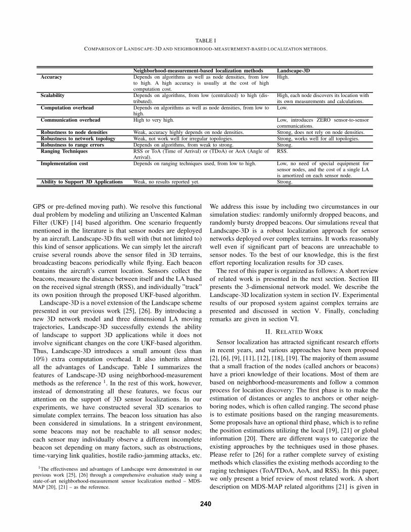
TABLE I

COMPARISON OF LANDSCAPE-3D AND NEIGHBORHOOD-MEASUREMENT-BASED LOCALIZATION METHODS.

Neighborhood-measurement-based localization methods Landscape-3DAccuracy Depends on algorithms as well as node densities, from low

to high. A high accuracy is usually at the cost of highcomputation cost.

High.

Scalability Depends on algorithms, from low (centralized) to high (dis-tributed).

High, each node discovers its location withits own measurements and calculations.

Computation overhead Depends on algorithms as well as node densities, from low tohigh.

Low.

Communication overhead High to very high. Low, introduces ZERO sensor-to-sensorcommunications.

Robustness to node densities Weak, accuracy highly depends on node densities. Strong, does not rely on node densities.Robustness to network topology Weak, not work well for irregular topologies. Strong, works well for all topologies.Robustness to range errors Depends on algorithms, from weak to strong. Strong.Ranging Techniques RSS or ToA (Time of Arrival) or (TDoA) or AoA (Angle of

Arrival).RSS.

Implementation cost Depends on ranging techniques used, from low to high. Low, no need of special equipment forsensor nodes, and the cost of a single LAis amortized on each sensor node.

Ability to Support 3D Applications Weak, no results reported yet. Strong.

GPS or pre-defined moving path). We resolve this functionaldual problem by modeling and utilizing an Unscented KalmanFilter (UKF) [14] based algorithm. One scenario frequentlymentioned in the literature is that sensor nodes are deployedby an aircraft. Landscape-3D fits well with (but not limited to)this kind of sensor applications. We can simply let the aircraftcruise several rounds above the sensor filed in 3D terrains,broadcasting beacons periodically while flying. Each beaconcontains the aircraft’s current location. Sensors collect thebeacons, measure the distance between itself and the LA basedon the received signal strength (RSS), and individually ”track”its own position through the proposed UKF-based algorithm.

Landscape-3D is a novel extension of the Landscape schemepresented in our previous work [25], [26]. By introducing anew 3D network model and three dimensional LA movingtrajectories, Landscape-3D successfully extends the abilityof landscape to support 3D applications while it does notinvolve significant changes on the core UKF-based algorithm.Thus, Landscape-3D introduces a small amount (less than10%) extra computation overhead. It also inherits almostall the advantages of Landscape. Table I summarizes thefeatures of Landscape-3D using neighborhood-measurementmethods as the reference 1. In the rest of this work, however,instead of demonstrating all these features, we focus ourattention on the support of 3D sensor localizations. In ourexperiments, we have constructed several 3D scenarios tosimulate complex terrains. The beacon loss situation has alsobeen considered in simulations. In a stringent environment,some beacons may not be reachable to all sensor nodes;each sensor may individually observe a different incompletebeacon set depending on many factors, such as obstructions,time-varying link qualities, hostile radio-jamming attacks, etc.

1The effectiveness and advantages of Landscape were demonstrated in ourprevious work [25], [26] through a comprehensive evaluation study using astate-of-art neighborhood-measurement sensor localization method – MDS-MAP [20], [21] – as the reference.

We address this issue by including two circumstances in oursimulation studies: randomly uniformly dropped beacons, andrandomly bursty dropped beacons. Our simulations reveal thatLandscape-3D is a robust localization approach for sensornetworks deployed over complex terrains. It works reasonablywell even if significant part of beacons are unreachable tosensor nodes. To the best of our knowledge, this is the firsteffort reporting localization results for 3D cases.

The rest of this paper is organized as follows: A short reviewof related work is presented in the next section. Section IIIpresents the 3-dimensional network model. We describe theLandscape-3D localization system in section IV. Experimentalresults of our proposed system against complex terrains arepresented and discussed in section V. Finally, concludingremarks are given in section VI.

II. RELATED WORK

Sensor localization has attracted significant research effortsin recent years, and various approaches have been proposed[2], [6], [9], [11], [12], [18], [19]. The majority of them assumethat a small fraction of the nodes (called anchors or beacons)have a priori knowledge of their locations. Most of them arebased on neighborhood-measurements and follow a commonprocess for location discovery: The first phase is to make theestimation of distances or angles to anchors or other neigh-boring nodes, which is often called ranging. The second phaseis to estimate positions based on the ranging measurements.Some proposals have an optional third phase, which is to refinethe position estimations utilizing the local [19], [21] or globalinformation [20]. There are different ways to categorize theexisting approaches by the techniques used in those phases.Please refer to [26] for a rather complete survey of existingmethods which classifies the existing methods according to theraging techniques (ToA/TDoA, AoA, and RSS). In this paper,we only present a brief review of most related work. A shortdescription on MDS-MAP related algorithms [21] is given in

240

the following subsection. Then, we take a glance at Bayesiantechniques for robot location estimations.

A. Multidimensional Scaling for Localization

Multidimensional scaling (MDS) has recently been success-fully used to resolve sensor localization problem [12], [20],[21]. MDS can be seen as a set of data analysis techniquesthat display the structure of distance-like data as a geometricalpicture. One main advantage in using MDS is that it can al-ways generate relatively high accurate position estimation evenbased on limited and error-prone distance information. Shanget al. first proposed MDS-MAP to use MDS in sensor locationproblem in [20]. MDS-MAP is a centralized algorithm, whichconsists of three steps:

1) Compute shortest paths between all pairs of nodes inthe sensor field. The shortest path distances are used toconstruct the distance matrix for MDS.

2) Apply classical MDS to the distance matrix, retainingthe first 2 (or 3) largest eigenvalues and eigenvectors toconstruct a 2D (or 3D) relative map.

3) Given sufficient anchors (3 or more for 2D, 4 or morefor 3D), transform the relative map to an absolute mapbased on the absolute positions of anchors.

MDS-MAP(P) [21] is an improved version of MDS-MAP.In MDS-MAP(P), individual nodes compute their own localmaps using their local information (the range of the local mapmay contain one-hop or two-hops neighbors) and then thelocal maps are merged to form a global map. If an optionalrefinement process is used for each local map before merging,the algorithm is called MDS-MAP(P,R).

As the state-of-the-art neighborhood-measurement basedapproach, MDS-MAP(P,R) has demonstrated impressive per-formance. However, as we will demonstrate in Section V,this method is quite sensitive to node densities and networktopologies, thus it is difficult to extend this method into asolution for applications deployed over complex 3D terrains.

B. Bayesian Techniques for Robot Localization

Bayesian techniques have been widely investigated in thecontext of robot localization [10]. Recently, grid based Markovlocalization [3], particle filter (a.k.a. sequential Monte Carlo)[7], real-time particle filters [15] have been proposed andshown to be successful for robot location estimation. ThoseBayesian techniques generally require intensive computationpower. There are substantial differences between robot lo-calization and sensor node positioning. First, while robotlocalization locates a robot in a predefined map, localizationin sensor networks works in a free space or unmapped terrain.Second, while a robot can acquire accurate range, bearing andorientation measurements to landmarks simultaneously withrelatively expensive equipment, small sensor nodes cannot.Third, a robot has much more computation power than a sensornode, and is able to execute complicated location algorithms.

Inspired by the techniques used for robot localization, Huand Evans [11] first proposed to use sequential Monte Carlo(SMC) method for mobile sensor node localization. Their

approach is called MCL (Monte Carlo Localization). Ourwork is different from theirs in several aspects. (1) MCLrequires a certain percentage of mobile anchors to work well,and it is designed for mobile sensor nodes. Landscape-3Dneeds only one mobile LA, and, it is mainly for static sensornetworks. (2) MCL utilizes only proximity measurement, withthe location estimation coarse-grained and bounded. In con-trast, Landscape-3D exploits range measurement and it is ableto acquire high accuracy. (3) With SMC requiring intensivecomputation power, upgrading MCL for range measurementsmight be impractical, because that would highly increase thecomputation cost of MCL.

III. NETWORK MODEL

We assume that the sensors are deployed randomly over a3-dimensional monitored area. As an example, Figure 1 showsa sensor network deployed over a monitored mountain area.Each sensor node has limited resources (CPU, battery, etc),and, is equipped with an omni-directional antenna. A locationassistant (LA) could be an airplane, a mobile robot, a vehicle,a balloon, etc. which is a choice up to the network designers.However, we do have the following minimal requirements onthe LA:

• The LA has moving ability, being able to move aroundthe sensor field.

• The LA is aware of its own location while it is moving,either through a GPS or a pre-defined moving path.

• The LA is able to broadcast beacons to sensor nodes;each beacon contains the LA’s current location and thetransmitting power used to transmit the beacon. In therest of the paper, the term beacon’s location is usedto reference the location of the LA when a beacon isbroadcasted.

The LA is free to leave after beacons are broadcasted. Duringthe process, each sensor passively listens to the beacons,estimating the distance between itself and the beacon basedon the measured RSS of the beacons. The localization processintroduces no sensor-to-sensor communication overhead. Thecommunication ability of sensor nodes to the LA is notassumed.

IV. LANDSCAPE-3D LOCALIZATION METHODOLOGY,MODEL AND ALGORITHM

A. Landscape-3D Localization Model

The key idea of Landscape-3D is to treat the sensor local-ization as a functional dual to the target tracking problems.In target tracking, one (or more) location-aware sensor nodeestimates the position (and optionally, velocity and accelera-tion) of a moving target based on the measurable distances orangle of arrives (AOAs). As a functional dual, each location-unaware sensor node utilizes the measured RSS to estimateits own position aided by the location-aware LA. From thisnovel perspective, the Landscape-3D system exploits varyingpositions of the LA and the corresponding sensor-to-LA dis-tances to dynamically determine the positions of sensor nodes.

241

LA

Area monitored by the sensor network

Sensor nodesBeacons broadcasted through RF signals

Fig. 1. An example sensor network deployed over 3D terrains.

Input: observation pairs

(location of beacon 1, distance1),(location of beacon 2, distance2),

…Output: position estimation,

(estimation1),(estimation2),

…

: Sensor node

: The LA moving trajectory

: Beacons broadcasted by the LA

: Distance between a beacon and the sensor node

Fig. 2. Landscape-3D methodology illustrated in 2-dimensions.

The sensor position is determined by solving the associatedstate evolvement and observation dynamics of the positions ofthe LA and the measured distances. Figure 2 illustrates theLandscape-3D localization methodology in a 2D manner.

For the localization problem described above, we define thestate variable as the 3D position of a specific sensor node. Thestate of the ith sensor node at the nth iteration is:

xi(n) = {xi1(n), xi2(n), xi3(n)}. (1)

And we have the following dynamic state and observationequations:

xi(n) = f(xi(n − 1)) + wi(n),yi(n) = g(xi(n)) + vi(n),

(2)

where f(·) and g(·) are state evolvement and observationfunctions respectively. f(·) may be linear or nonlinear de-pending on application scenarios, while g(·) is usually highlynonlinear. wi(n) and vi(n) are state and observation noisesequences.

Here let us consider the static sensor localization, wherepositions of the sensors remain unchanged after deployment.That is, the state dynamics f(·) governing the sensor positions

are simply the identity functions:

xi(n + 1) = xi(n) + wi(n), (3)

where wi(n) models the small position perturbation due to thewind or other environmental effects. Note that our algorithmcan be extended to mobile sensors by incorporating time-varying state dynamics, which is one of our future researchlines.

The state dynamics on the LA are controlled or programmedin advance, and can be delivered to sensor nodes. Equippedwith accurate GPS, the LA knows its current location. Thecurrent position can be transmitted through RF signal to thesensors. The following observation model is used:

yi(n) =√

(∆xi1(n))2 + (∆xi2(n))2 + (∆xi3(n))2 + vi(n).(4)

Here ∆xi1(n) = xb1(n)− xi1(n), ∆xi2(n) = xb

2(n)− xi2(n),∆xi3(n) = xb

3(n) − xi3(n); and (xb1(n), xb

2(n), xb3(n)) is the

current 3D position of the LA, measured using GPS or con-trolled by the pre-defined path. vi(n) models the observationerror, which usually comes from the RF distance estimationsor the perturbations to the LA positions. We assume wi(n)and vi(n) are zero-mean uncorrelated noise processes.

B. Dynamic State Estimation Via Unscented Kalman Filter

The Landscape-3D localization scheme aims at improvingthe sensor localization by iteratively updating the positionestimates with the current observations. For the system modeldefined in the previous section, on-line state estimation hasto be performed. Kalman filters and their variants have beendesigned for this purpose, but their actual performance de-pends heavily on the evolvement and observation equations,as well as the nature of the noise sequences. Due to thenonlinearity of the observation equation, which is the rooted-sum-of-squares of position difference, standard Kalman filter(KF) is not suitable to our localization model. Neither is theextended Kalman filter (EKF), the first-order approximationto the nonlinear system that is often plagued by the empiricallinearization. For the nonlinear observation function g(·),the unscented transformation (UT) [13], [17] is an elegantapproach to providing higher-order approximations. It canaccurately compute the statistical mean and variance up tothe third-order of Taylor series expansion of g(·) for Gaus-sian noise sequences, or the second-order for arbitrary noisedistributions. Higher-order approximation can also be capturedwith extended algorithms [14]. At the same time, UT uses thesame order of calculations as linearization. The above analysishas driven us to utilize unscented Kalman filter (UKF) [13] inour Landscape-3D scheme.

The basic idea of UT is to represent the state distributionby a minimal set of carefully chosen sample points (sigmapoints). The UKF embeds the UT into the Kalman Filter’srecursive prediction and update structure. The detailed theo-retical background of UT and UKF can be found in our onlinetechnical report [26]. We skip the details here, however, dueto the space limitation.

242

Start

Calibration for RSS-based distance measurement (pre-deployment, optional)

On-line position estimation?

On-line position estimation

Estimate the distance from the sensor to the beacon

Apply UT to generate sigma points

Utilizing sigma points and new observation to predict and update

mean and variance

Wai

tfo

rn

ext

beaco

n?

Collect observation-pairs

Estimate the distance from the sensor to the beacon

Store the observation-pair (beacon location, distance)

Wai

tfo

rn

ext

beaco

n?

Apply UT to generate sigma points

Utilizing sigma points and new observation-pair to predict and

update mean and variance

Hav

enex

tO

bse

rvat

ion

-pair

?

Initialize position, state and observation noise variances

End

Receiving a beacon

Receiving a beacon

Take one observation-pair

Yes

Yes

Yes

Yes

No

No

No

No

Off-line position estimation

Initialize position, state and observation noise variances

Fig. 3. Landscape-3D’s UKF-based localization algorithm.

C. UKF-based Algorithm

Figure 3 outlines the UKF-based localization algorithm. Asshown in the picture, the algorithm has an optional calibra-tion procedure, which could be done before sensor nodesare deployed. The purpose of the calibration is to improvethe accuracy of RSS-based distance measurements [23]. Thecore of the algorithm is the iteration of state prediction andupdating, which could be done either on-line or off-line. Whenthe iterations are done off-line, each sensor node first collectsall the observation-pairs (each of which contains a beacon’sposition and its distance from the sensor node), then executesthe UKF loops to update its location estimation exploiting theconstraints increasing added by each observation-pair. The off-line version of the algorithm does not have a time constraint 2

on each iteration of state prediction/updating, thus it is moresuitable for sensor nodes that have lower computation power.However, Each sensor node needs to have several kilo-bytesmemory 3 to temporarily store the observation-pairs, which isa reasonable requirement for most sensor applications.

Since each sensor individually calculates its own location,the computation complexity of Landscape-3D is independentof the network size. In another words, the computation over-head is ©(n) (n is the number of sensors in the network) interms of the whole network or ©(1) in terms of each sensor.Unlike neighborhood-measurement based location methods,

2The on-line version requires the iteration for one beacon be finished beforethe next beacon comes.

3As shown in the later section, for the example scenarios, 240 beaconsare enough for Landscape-3D to work well. If we use 6 bytes to represent abeacon’s location (3D), 2 bytes to represent the distance from the beacon toa sensor node, the observation-pair for each beacon will consume 8 memorybytes to store. for 240 beacons, we need totally 1920 bytes.

where sensors usually communicate with each other massively(for ranging measurements, and for exchanging location esti-mations to refine the results), Landscape-3D introduces zerosensor-to-sensor communications. The communication fromsensor nodes to the LA is not needed as well. Consider-ing communications usually are more energy-consuming thancomputations, this is an important advantage of Landscape-3D.

V. EXPERIMENTAL RESULTS

In our experiments, we run Landscape-3D on various 3Dterrain models in Matlab. Since previous approaches onlyreport results for 2-dimensional localizations, it is hard tocompare the performance of Landscape-3D with them for3D cases. As a way around, besides the complex 3D terrainmodels, we also include some results for flat (2D) terrainmodels that have irregular topologies. For the 2D terrain mod-els, we compare the performance of Landscape-3D with themost well-known neighborhood-measurement based approach– MDS-MAP. For comparison purpose, both algorithms areinterfaced to the localization simulation toolkit designed as apart of the Berkeley’s Calamari project [24].

Table II summarizes the metrics and parameters used in oursimulations. We assume distance measurements have Gaussiannoise [20], [21]. A random noise is added to the true distanceas following:

d̂ = d ∗ (1 + randn(1) ∗ range error), (5)

where d is the true distance, d̂ is the measured distance,range error is a value between [0,1], and randn(1) is astandard normal random variable.

A. Flat Terrains with Irregular Topologies

In this experiment, we use MDS-MAP as the referenceto evaluate the performance of Landscape-3D for a sensornetwork deployed over a flat terrain. We use a square sensorfield (1000 by 1000) with (0,0), (0, 1000), (1000, 1000), and(1000, 0) as its four corners. To construct an irregular networktopology, we assume there is a lake in the middle of the sensorfield. The lake is in round shape and has a radius of 400with (500, 500) as its center. 200 sensor nodes are randomlydeployed over the sensor field around the lake. We let anairplane be the LA. For this scenario, the LA hovers overthe sensor field on a 2D plane parallel to the sensor field. Theheight of the airplane is a constant value, for which we used100 feet. The LA periodically broadcasts beacon samples tosensor nodes. In this scenario, the location of the LA at timestep n (n ≥ 1) is simply:

xb1(n) = c1 + RLA cos(2π/samples per round ∗ (n − 1)),

xb2(n) = c2 + RLA sin(2π/samples per round ∗ (n − 1)), (6)

xb3(n) = c3,

where c1, c2, and c3 are 500, 500, and 100 respectively, andRLA is 700. We assume that the LA broadcasts same number(samples per round) of beacon samples in each round. For

243

TABLE II

METRICS AND PARAMETERS USED IN EVALUATIONS.

Metrics and Parameters Definition/Explanation

Metrics Accuracy (position error) The accuracy of sensor positioning is presented as the average distance between estimatedpositions to the true positions.

Computation Overhead For comparison purpose, we report the CPU time consumed (per sensor node) by positionalgorithms in our simulations. All simulations are conducted on a DELL precision 670workstation (Intel Xeon 3.0GHz CPU, 2 GB DDR-2 memory).

Parameters

Range Error The error introduced in distance estimation based on RSS. It has a value between [0.1] inour model for noisy RSS-based distance measurement described in equation (5).

Total Samples The total number of beacons broadcasted by the LA.Samples Per Round In all the simulations reported in this paper, we have used simple LA moving trajectories, in

which the LA simply hovers around the sensor field and broadcasts equal number of beaconsper round.

Connectivity The number of one-hop-neighbors of a sensor node. In simulations, the average connectivity ofa network could be changed by varying the sensor radio range. Landscape-3D is independentof this parameter.

0 100 200 300 400 500 600 700 800 900 10000

100

200

300

400

500

600

700

800

900

1000

0 100 200 300 400 500 600 700 800 900 10000

100

200

300

400

500

600

700

800

900

1000

0 100 200 300 400 500 600 700 800 900 10000

100

200

300

400

500

600

700

800

900

1000

(a) Original Map (b) Result of MDS-MAP(P,R) (c) Result of Landscape-3D

Fig. 4. Comparison of Landscape-3D and MDS-MAP for Flat terrain with irregular topology

TABLE III

COMPARISON OF LANDSCAPE-3D AND MDS-MAP(P,R) FOR A FLAT TERRAIN WITH IRREGULAR TOPOLOGY.

Algorithm Parameters Resultssensor radio range connectivity range error position error CPU time per node

One trail MDS-MAP(P,R) 200 25.712 10% 106.764 0.544 sec.Landscape-3D N/A N/A 10% 11.216 0.143 sec.

Another trailMDS-MAP(P,R) 250 33.130 10% 58.097 1.249 sec.Landscape-3D N/A N/A 10% 11.712 0.141 sec.

The average of MDS-MAP(P,R) 200 26.016 10% 115.357 0.568 sec.another 1000 trails Landscape-3D N/A N/A 10% 11.092 0.143 sec.

the simulations reported here, we use 240 total beacon sampleswith 15 samples per round.

For the simulation of MDS-MAP, we have used MDS-MAP(P,R), which is the distributed version of MDS-MAPwith a refinement procedure. The performance of MDS-MAPalgorithm depends on the network connectivity. Generally, thehigher the connectivity, the higher the accuracy and compu-tation cost. In simulations, the connectivity could be changedby varying the sensor’s radio range (Since sensor nodes arerandomly deployed, even with the same sensor radio range, theconnectivity could be slightly different in different trials.). Inthe experiments for MDS-MAP(P,R), 5% nodes are assumedas anchor nodes (with known locations).

We demonstrate the localization results of Landscape-3Dand MDS(P,R) of one trail in Figure 4, in which (a) showsthe original map of the sensors, (b) shows the result of MDS-

MAP(P,R), and (c) shows the result of Landscape-3D. In thefigures, small circle represent the original location of sensornodes, while small arrows point to the estimated positions.As clearly shown in the figures, MDS-MAP(P,R) does notwork well for the case although the average connectivity ofthe network is as high as 25.7. More details of the comparisonis given in Table III, in which trail one is the trail reported inFigure 4, trail two is another trail with a higher connectivity.To eliminate the effect of occasionality, the average of another1000 trails (sensors are randomly re-deployed for each trail) isalso reported in the table. Landscape-3D yields much higheraccuracy with less computation overhead.

B. Complex Terrains with Complete Beacon Set

In this experiment, we evaluate Landscape-3D against vari-ous complex 3D terrains. Similar to the previous experiment,

244

0

500

1000

0200

400600

8001000

−200

0

200

0

500

1000

0200

400600

8001000

−200

0

200

0

500

1000

0200

400600

8001000

−200

0

200

(a) Result for 10% range error (b) Result for 20% range error (c) Result for 30% range error

Fig. 5. The result of Landscape-3D for complex terrain 1 – Valley

0200

400600

8001000

0

500

1000

−300

−200

−100

0

100

200

300

0200

400600

8001000

0

500

1000

−300

−200

−100

0

100

200

300

0200

400600

8001000

0

500

1000

−300

−200

−100

0

100

200

300

(a) Result for 10% range error (b) Result for 20% range error (c) Result for 30% range error

Fig. 6. The result of Landscape-3D for complex terrain 2 – Mountain

0200

400600

8001000

0

500

1000

−300

−200

−100

0

100

200

300

0200

400600

8001000

0

500

1000

−300

−200

−100

0

100

200

300

0200

400600

8001000

0

500

1000

−300

−200

−100

0

100

200

300

(a) Result for 10% range error (b) Result for 20% range error (c) Result for 30% range error

Fig. 7. The result of Landscape-3D for complex terrain 3 – Mountains and valleys

200 sensor nodes are randomly deployed over a 1000 by1000 sensor field. The sensor field used in this experiment,however, is not a flat terrain. Three scenarios are constructed toemulate a terrain with a valley, a terrain with a mountain, anda terrain with mountains and valleys respectively. To providereferences in the third dimension, we let the LA vary itsheight when it hovers around the sensor field. Again, a simpletrajectory is employed. During the first half of the procedure(of broadcasting beacons), the LA spirals upwards. During thesecond half of the procedure, it spirals downwards. We usethe same LA trajectory for all three scenarios (terrains). Thelocation of the LA at time step n (n ≥ 1) could be describedusing the same equation as (6), except the formula for xb

3(n)is changed as the follow:

xb3(n) =

8<:

c3 if n = 1;xb

3(n − 1) + 10 if 1 < n ≤ total samples/2;xb

3(n − 1) − 10 if n > total samples/2.

In this experiment, we assume every sensor node is able toreceive the complete beacon set. Figures 5, 6, and 7 demon-strate the result of Landscape-3D under three scenarios withdifferent range errors. As shown in the figures, Landscape-3Dworks pretty well for all the three scenarios. Not surprisingly,we can see that the position error increases with the rangeerror.

C. Complex Terrains with Incomplete Beacon Set

Assuming every sensor node be able to receive all thebeacons may be too optimistic. In real applications, each

245

0200

400600

8001000

0

500

1000

−300

−200

−100

0

100

200

300

0

20

40

60

80

100

120

0 20 40 60 80 100

Avera

ge Po

sition

Error

Drop rate (%)

AccuracyUniformly dropped

Bursty dropped

0

0.05

0.1

0.15

0.2

0 20 40 60 80 100

CPU T

ime Pe

r Node

(secon

ds)

Drop rate (%)

Computation OverheadUniformly dropped

Bursty dropped

(a) Result for (b) Accuracy: (c) Computation overhead:

60% beacons bursty-dropped uniformly-dropped vs. bursty-dropped uniformly-dropped vs. bursty-dropped

Fig. 8. The result of Landscape-3D with incomplete beacon set (with 20% range error)

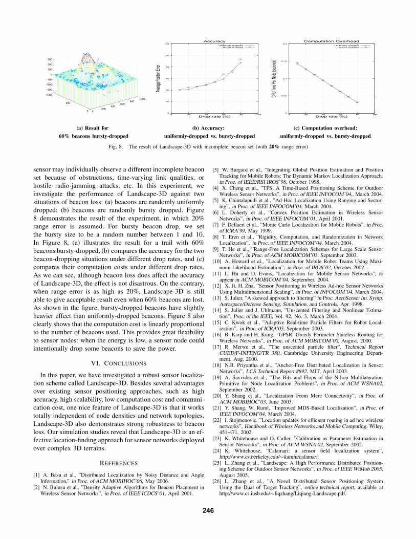
sensor may individually observe a different incomplete beaconset because of obstructions, time-varying link qualities, orhostile radio-jamming attacks, etc. In this experiment, weinvestigate the performance of Landscape-3D against twosituations of beacon loss: (a) beacons are randomly uniformlydropped; (b) beacons are randomly bursty dropped. Figure8 demonstrates the result of the experiment, in which 20%range error is assumed. For bursty beacon drop, we setthe bursty size to be a random number between 1 and 10.In Figure 8, (a) illustrates the result for a trail with 60%beacons bursty-dropped, (b) compares the accuracy for the twobeacon-dropping situations under different drop rates, and (c)compares their computation costs under different drop rates.As we can see, although beacon loss does affect the accuracyof Landscape-3D, the effect is not disastrous. On the contrary,when range error is as high as 20%, Landscape-3D is stillable to give acceptable result even when 60% beacons are lost.As shown in the figure, bursty-dropped beacons have slightlyheavier effect than uniformly-dropped beacons. Figure 8 alsoclearly shows that the computation cost is linearly proportionalto the number of beacons used. This provides great flexibilityto sensor nodes: when the energy is low, a sensor node couldintentionally drop some beacons to save the power.

VI. CONCLUSIONS

In this paper, we have investigated a robust sensor localiza-tion scheme called Landscape-3D. Besides several advantagesover existing sensor positioning approaches, such as highaccuracy, high scalability, low computation cost and communi-cation cost, one nice feature of Landscape-3D is that it workstotally independent of node densities and network topologies.Landscape-3D also demonstrates strong robustness to beaconloss. Our simulation studies reveal that Landscape-3D is an ef-fective location-finding approach for sensor networks deployedover complex 3D terrains.

REFERENCES

[1] A. Basu et al., ”Distributed Localization by Noisy Distance and AngleInformation,” in Proc. of ACM MOBIHOC’06, May 2006.

[2] N. Bulusu et al., ”Density Adaptive Algorithms for Beacon Placement inWireless Sensor Networks”, in Proc. of IEEE ICDCS’01, April 2001.

[3] W. Burgard et al., ”Integrating Global Position Estimation and PositionTracking for Mobile Robots: The Dynamic Markov Localization Approach.in Proc. of IEEE/RSI IROS’98, October 1998.

[4] X. Cheng et al., ”TPS, A Time-Based Positioning Scheme for OutdoorWireless Sensor Networks”, in Proc. of IEEE INFOCOM’04,, March 2004.

[5] K. Chintalapudi et al., ”Ad-Hoc Localization Using Ranging and Sector-ing”, in Proc. of IEEE INFOCOM’04, March 2004.

[6] L. Doherty et al., ”Convex Position Estimation in Wireless SensorNetworks”, in Proc. of IEEE INFOCOM’01, April 2001.

[7] F. Dellaert et al., ”Monte Carlo Localization for Mobile Robots”, in Proc.of ICRA’99, May 1999.

[8] T. Eren et al., ”Rigidity, Computation, and Randomization in NetworkLocalization”, in Proc. of IEEE INFOCOM’04, March 2004.

[9] T. He et al., ”Range-Free Localization Schemes for Large Scale SensorNetworks”, in Proc. of ACM MOBICOM’03, September 2003.

[10] A. Howard et al., ”Localization for Mobile Robot Teams Using Maxi-mum Likelihood Estimation”, in Proc. of IROS’02, October 2002.

[11] L. Hu and D. Evans, ”Localization for Mobile Sensor Networks”, toappear in ACM MOBICOM’04, September, 2004.

[12] X. Ji, H. Zha, ”Sensor Positioning in Wireless Ad-hoc Sensor NetworksUsing Multidimensional Scaling”, in Proc. of INFOCOM’04, March 2004.

[13] S. Julier, ”A skewed approach to filtering” in Proc. AeroSense: Int. Symp.Aerospace/Defense Sensing, Simulation, and Controls, Apr. 1998.

[14] S. Julier and J. Uhlmann, ”Unscented Filtering and Nonlinear Estima-tion”, Proc. of the IEEE, Vol. 92, No. 3, March 2004.

[15] C. Kwok et al., ”Adaptive Real-time Particle Filters for Robot Local-ization”, in Proc. of ICRA’03, September 2003.

[16] B. Karp and H. Kung, ”GPSR: Greedy Perimeter Stateless Routing forWireless Networks”, in Proc. of ACM MOBICOM’00, August, 2000.

[17] R. Merwe et al., ”The unscented particle filter”. Technical ReportCUED/F-INFENG/TR 380, Cambridge University Engineering Depart-ment, Aug. 2000.

[18] N.B. Priyantha et al., ”Anchor-Free Distributed Localization in SensorNetworks”, LCS Technical Report #892, MIT, April 2003.

[19] A. Savvides et al., ”The Bits and Flops of the N-hop MultilaterationPrimitive for Node Localization Problems”, in Proc. of ACM WSNA02,September 2002.

[20] Y. Shang et al., ”Localization From Mere Connectivity”, in Proc. ofACM MOBIHOC’03, June 2003.

[21] Y. Shang, W. Ruml, ”Improved MDS-Based Localization”, in Proc. ofIEEE INFOCOM’04, March 2004.

[22] I. Stojmenovic, ”Location updates for efficient routing in ad hoc wirelessnetworks”, Handbook of Wireless Networks and Mobile Computing, Wiley,451-471, 2002.

[23] K. Whitehouse and D. Culler, ”Calibration as Parameter Estimation inSensor Networks”, in Proc. of ACM WSNA’02, September 2002.

[24] K. Whitehouse, ”Calamari: a sensor field localization system”,http://www.cs.berkeley.edu/∼kamin/calamari.

[25] L. Zhang et al., ”Landscape: A High Performance Distributed Position-ing Scheme for Outdoor Sensor Networks”, in Proc. of IEEE WiMob 2005,August 2005.

[26] L. Zhang et al., ”A Novel Distributed Sensor Positioning SystemUsing the Dual of Target Tracking”, online technical report, available athttp://www.cs.iusb.edu/∼liqzhang/Liqiang-Landscape.pdf.

246