3D Localization and Wireless Sensor Networks

Thesis submitted in partial fulfillment of

requirements for the degree of

Master of Science by Research

in ELECTRONICS AND COMMUNICATIONS

by

BalaKrishna Pillalamarri

200950062

Email: balakrishna.p@research.iiit.ac.in

International Institute of Information Technology, Hyderabad(Deemed to be University)

Hyderabad - 500 032, INDIA May 2017

Copyright c©Balakrishna Pillalamarri 2017All Rights Reserved

International Institute of Information TechnologyHyderabad,India

Certificate

It is certified that the work contained in this thesis, “3D Localization andWireless Sensor Networks” submitted by Balakrishna Pillalamarri has beencarried out under my supervision and is not submitted elsewhere for a degree.

Adviser: Dr. Rama Murthy Garimella

22/05/2017Date

Dedicated to My Guru Sri Sri Sri Swayam Prakasananda SachidanandaSaraswathi MahaSwamiji

3

Acknowledgments

I am lucky to work with Dr Rama Murthy Garimella. My journey in IIIT-Hyderabad has been a journey worth it. It could not have been so without thesupport of many people. As I submit my MS thesis, I want to offer my gratitudeto all those people who helped me in successfully completing this journey. First ofall, I want to thank my guide Prof. Rama Murthy Garimella, for accepting me asa student and constantly guiding me.

His guidance has helped me improve not only as a researcher but also as aperson. I can never thank him enough for providing me support at my difficulttimes and helping me move forward.

I am thankful to everyone in SPCRC for providing such a positive work environ-ment. Many thanks to Tejaswini, Sumit, Viswanath, Srikanth, Kunal, Chandan,Priyanaka for all the help, discussions, study group sessions and support. Thanksto Prof. Rama Murthy for remaining by my side rock steady throughout thisjourney and for being my guide and mentor through my ups and downs.

I could not have accomplished it without the support and understanding of mywife . I wish to thank my mom, dad and my wife and kids for being my constantsupport and motivation

The most valuable person without whose support I would have not come to thisstage is my beloved friend Dr.Balagangadhar Bathula, Research Associate, AT&TBell Labs, USA. Last, but not the least, thanks to IIIT community for giving mesuch a beautiful campus and environment to grow.

4

Abstract

Indoor positioning is gaining momentum for its various applications. As weknow that Global Positioning System (GPS) does not work well indoors, whiletodays more sensitive GPS chips can sometimes get a location fix (via receivingsignals from enough satellites to determine a location) inside a building. The re-sulting location is typically not accurate enough to be useful. The signals from thesatellites are attenuated and scattered by roofs, walls and other objects. Besides,the error range of many GPS chips (tennis court) can be larger than the indoorspace itself (small grocery store)! Some indoor positioning solutions work similarto GPS.

Many companies tap into Wi-Fi signals that are all around us - including whenwe are indoors. With a good map of the locations of the access points, a Wi-Fireceiver like a cell phone can be located even indoors.

Any application that would depend on indoor positioning may need an exactlocation. This work on indoor localization in 3D using spherical co-ordinateswould have an edge to all the future needs. A combination of Pico, Femto, Wi-Fi,otherwise termed as hybrid localization techniques are used in conjunction withleveling and sectoring. Leveling and sectoring are discussed using base station andWi-Fi access points and the received signal strength (RSS) finger prints are usedto aid in precise localization. Indoor localization applied to physical analytics isalso discussed.

This thesis work also focuses in an improvement over our above discussed worksin terms of achieving more accuracy and reduction of delay in the Wireless SensorNetworks (WSNs). This is achieved by using the Received Channel Power Indi-cator (RCPI) in contrast to RSS. We assume that RCPI shall be used by all chipvendor for all the Wi-Fi devices coming into the market due to its precise way ofmeasuring the Received signal power.

This work also focuses on Wireless Sensor Networks (WSN) with respect tothe need for optimizing the parallel distributed computational architecture.It alsodiscussed how it can be acheived using our proposed model. This gains impor-tance as identification of an event in WSNs should be done as fast as possible byminimizing the delay.

Optimizing the grid based architecture for time complexity, transmission delayand fault tolerance in computing the fusion functions, our work also focuses onlocalizing an event in an outdoor WSN and respond to the event based on theneed as soon as possible.

Hence our overall work on 3D localization and wireless sensor networks helpsus localize events in both indoor as well as outdoor with reduced time-complexityas well as delay parameters.

Contents

Acknowledgements 4

1 Introduction 11.1 Overview . . . . . . . . . . . . . . . . . . . . . . . . . . . . . . . . 11.2 Problem Statement . . . . . . . . . . . . . . . . . . . . . . . . . . . 2

1.2.1 Contribution of Thesis . . . . . . . . . . . . . . . . . . . . . 31.3 Concept of Localization . . . . . . . . . . . . . . . . . . . . . . . . 31.4 Thesis Organization . . . . . . . . . . . . . . . . . . . . . . . . . . . 3

2 Precise Positioning in 3D Using Spherical Co-ordinates 42.1 Introduction . . . . . . . . . . . . . . . . . . . . . . . . . . . . . . . 42.2 Related Work . . . . . . . . . . . . . . . . . . . . . . . . . . . . . . 62.3 Precise Positioning Algorithm . . . . . . . . . . . . . . . . . . . . . 6

2.3.1 Horizontal Positioning . . . . . . . . . . . . . . . . . . . . . 72.3.2 Vertical Positioning . . . . . . . . . . . . . . . . . . . . . . . 82.3.3 Machine Learning Techniques into Positioning . . . . . . . . 8

2.4 Indoor Localization applied to Physical Analytics . . . . . . . . . . 92.5 Localization Accuracy . . . . . . . . . . . . . . . . . . . . . . . . . 122.6 Application of Proposed Approach for Outdoor Localization . . . . 122.7 Improved Accuracy using RCPI . . . . . . . . . . . . . . . . . . . . 122.8 Conclusion . . . . . . . . . . . . . . . . . . . . . . . . . . . . . . . . 132.9 References . . . . . . . . . . . . . . . . . . . . . . . . . . . . . . . . 13

3 Grid of Wireless Sensors:Distributed Computation 153.1 Introduction . . . . . . . . . . . . . . . . . . . . . . . . . . . . . . . 153.2 Distributed Network Architecture for Primitive Recursive Functions 16

3.2.1 Problem Statement . . . . . . . . . . . . . . . . . . . . . . . 163.2.2 Primitive Recursive Functions . . . . . . . . . . . . . . . . . 163.2.3 Grid based Network Architecture . . . . . . . . . . . . . . . 173.2.4 Fault Tolerance . . . . . . . . . . . . . . . . . . . . . . . . . 193.2.5 Probability of Error in Maximum Calculation . . . . . . . . 22

3.3 Distributed Network Architecture for Median . . . . . . . . . . . . 223.3.1 Problem Statement . . . . . . . . . . . . . . . . . . . . . . . 223.3.2 Tree based Network Architecture . . . . . . . . . . . . . . . 223.3.3 Computational Complexity of the Proposed Architecture . . 253.3.4 Time Delay of the Proposed Tree based Architecture for Median 25

3.4 Applications . . . . . . . . . . . . . . . . . . . . . . . . . . . . . . . 263.4.1 Dynamic Speed Boards . . . . . . . . . . . . . . . . . . . . . 26

i

3.4.2 Dynamic Time Estimate . . . . . . . . . . . . . . . . . . . . 273.4.3 More Accurate Time Estimate . . . . . . . . . . . . . . . . . 273.4.4 Itinerary Planning . . . . . . . . . . . . . . . . . . . . . . . 283.4.5 Coloring Nodes . . . . . . . . . . . . . . . . . . . . . . . . . 293.4.6 Possible Improvements in Google Maps . . . . . . . . . . . . 30

3.5 Conclusion . . . . . . . . . . . . . . . . . . . . . . . . . . . . . . . . 303.6 References . . . . . . . . . . . . . . . . . . . . . . . . . . . . . . . . 31

4 Outdoor Navigation: Efficient Order Statistics computation 324.1 Introduction . . . . . . . . . . . . . . . . . . . . . . . . . . . . . . . 324.2 Localization . . . . . . . . . . . . . . . . . . . . . . . . . . . . . . . 334.3 Order Statistics . . . . . . . . . . . . . . . . . . . . . . . . . . . . . 354.4 Efficient Computation In Grid Based Architecture . . . . . . . . . . 384.5 Temporal Statistics . . . . . . . . . . . . . . . . . . . . . . . . . . . 394.6 Conclusion . . . . . . . . . . . . . . . . . . . . . . . . . . . . . . . . 404.7 References . . . . . . . . . . . . . . . . . . . . . . . . . . . . . . . . 40

5 Conclusion and Future work 415.1 Conclusion . . . . . . . . . . . . . . . . . . . . . . . . . . . . . . . . 415.2 Future Work . . . . . . . . . . . . . . . . . . . . . . . . . . . . . . . 41

ii

List of Figures

2.1 Spherical Co-ordinate system . . . . . . . . . . . . . . . . . . . . . 52.2 Leveling and Sectoring in a Horizontal Plane . . . . . . . . . . . . 72.3 Set up showing the sector formation by BS and AP. . . . . . . . . . 92.4 Spherical Co-ordinates applied to position an object . . . . . . . . . 102.5 Flow Chart . . . . . . . . . . . . . . . . . . . . . . . . . . . . . . . 11

3.1 Example of a path; from source to destination . . . . . . . . . . . . 183.2 Hierarchy of grid architecture . . . . . . . . . . . . . . . . . . . . . 203.3 Proposed Architecture showing the Row links . . . . . . . . . . . . 203.4 Fault Tolerance scenarios . . . . . . . . . . . . . . . . . . . . . . . . 213.5 Tree like Architecture . . . . . . . . . . . . . . . . . . . . . . . . . . 223.6 Original Heap to Reduced Head Tree . . . . . . . . . . . . . . . . . 233.7 Example 1: Median of Medians . . . . . . . . . . . . . . . . . . . . 243.8 Example 2: Median of Medians . . . . . . . . . . . . . . . . . . . . 243.9 Example figure for Heap Sort . . . . . . . . . . . . . . . . . . . . . 253.10 Dynamic Time Estimate . . . . . . . . . . . . . . . . . . . . . . . . 273.11 More Accurate Time Estimate . . . . . . . . . . . . . . . . . . . . . 283.12 Itinerary Planning . . . . . . . . . . . . . . . . . . . . . . . . . . . 29

4.1 Localization problem being addressed . . . . . . . . . . . . . . . . . 334.2 Grid based architecture . . . . . . . . . . . . . . . . . . . . . . . . . 344.3 Line architecture . . . . . . . . . . . . . . . . . . . . . . . . . . . . 36

iii

List of Tables

2.1 Power leveling with the corresponding RSS levels . . . . . . . . . . 82.2 Major conventions. Legend: Eastwards (E) Northwards (N) Upwards (U). 9

4.1 List of values of kpivot for few values of N. . . . . . . . . . . . . . . 37

iv

Chapter 1

Introduction

1.1 Overview

Indoor Localization is gaining more prominance in today’s applications.With theadvent of smartphones enabled with WI-FI and other technologies,it gives moreways to solve the challenges in indoor space.GPS does not work well indoors: Whiletodays more sensitive GPS chips can sometimes get a fix (receive signals fromenough satellites to determine a location) inside a building, the resulting locationis typically not accurate enough to be useful. The signals from the satellites areattenuated and scattered by roofs, walls and other objects. Besides, the errorrange of many GPS chips (tennis court) can be larger than the indoor space itself(small grocery store)!

Some indoor positioning solutions work similar to GPS: Locata, an Australiancompany, offers beacons that send out signals that cover large areas and can pene-trate walls. Locata receivers work similarly to how GPS receivers work. The U.S.Department of Defense is an early Locata user. Nokia uses beacons that send outBluetooth signals. While any Bluetooth device can read them, they only cover afew square meters.

Many companies tap into Wi-Fi signals that are all around us - including whenwe are indoors. With a good map of the locations of the access points, a Wi-Fireceiver like a cell phone can be located even indoors.

RFID and inertial systems work very differently: Passive radio frequency iden-tification tags (RFIDs) prompt a transaction when they pass near a sensor. Forexample, a closed door prompts the user to swipe the card to pass. Doors orgates force users into a queue or to slow down for the sensor to work properly.These passive systems detail only that a person or object entered a room; they donot provide detailed location information within the room. Active RFID tags areself-powered and regularly send out signals to receivers within the area of interest.This is the reverse of GPS. Knowing the location of the receiving sensors allows foraccurate indoor locating in near real-time. Solutions that use inertial measurementwork only if a starting location is known. With that information collected, thesesensors use accelerometers, gyroscopes and other sensors including clocks to trackorientation and distance to keep track of location in near real-time. The latestinertial solution, from DARPA, is a chip smaller than a penny (press release).

Indoor positioning detects the location of a person or object, but not always its

1

orientation or direction: While indoor positioning systems can determine location,many need additional information to determine which way a person or object isfacing. That can make providing directions or pitching a product in a store morechallenging. The addition of an electronic compass to a receiver (many cell phonesnow have them), or a microelectromechanical systems (MEMS) orientation sensoror a prompt to turn toward a particular direction (to scan a bar code or QR codeon a poster, for example) can provide more information regarding orientation.

The best solution for indoor and outdoor positioning may be a hybrid: Nosingle solution works perfectly in all environments. For that reason devices maysupport more than one positioning solution and switch between them as needed.Todays mobile phones use GPS (when its turned on) outdoors but may switch toWi-FI positioning (when its turned on) when the signal is weak, such as when anindividual goes indoors. Indoor location and commerce solution provider aisle 411taps into both Wi-Fi and MEMS sensors for its retail store offerings.

Indoor positioning is in demand for a variety of uses: While the goal of indoorpositioning for some users, notably hospitals and malls, is to provide navigationaid, others want to use indoor positioning to better market to customers, providejust-in-time information via audio for tours, offer video or augmented reality expe-riences or connect people of interest in proximity to one another. The U.S. FederalCommunications Commission hopes to use indoor positioning to provide timelierand more effective emergency services (see below).

Major tech players are working in the indoor space: Apple, Google and Mi-crosoft are all exploring the use of indoor positioning. At this time the effort isfocusing on both indoor positioning technologies and creating the basemaps thatwill make such solutions more valuable.

The Federal Communications Commission (FCC) is looking at indoor position-ing to enhance emergency response: Results of a study conducted in late 2012 andpublished March 14, 2013 by the FCCs Communications Security, Reliability andInteroperability Council (CSRIC) suggests a current baseline for indoor position-ing for use in emergency response. Three different vendors, using three differentindoor technologies, participated (summary).One key concern is determining ver-tical location, that is, on which floor a person is standing in a multilevel building.The FCC report concludes: “While the location positioning platforms tested pro-vided a relatively high level of yield, as well as improved accuracy performance,the results clearly indicate additional development is required.”

Indoor positioning requires indoor maps: Locating a person or device indoors isonly half of the solution. For the location to be meaningful for navigation or otherpurposes, service providers need accurate indoor maps. Theres a new industrycreating those data.

1.2 Problem Statement

Wireless Communications is a vast area, posing significant challenges in various di-rections. While there are many open research problems unsolved from many years,the technical revolution, we are witnessing with the explosion of smart phones hasleft the wireless research community with very interesting problems. Outdoor po-sitioning is achieved with the help of GPS (Global Positioning Systems). On the

2

other hand, indoor positioning i.e., positioning of smart phone or a wireless sen-sor node precisely within a building has always been a challenge especially due tomultipath and fading charectersitics of a wireless signal. To overcome this thereare lot of techniques being proposed by researchers, and some of them include 2Dlocalization as well as 3D, but always have some degree of error.

1.2.1 Contribution of Thesis

(A) To overcome and minimize the error in localizing a node or an event wepropose a new technique which shall increase the accuracy of the positioning andlocalization in 3D.

(B) The network architectures formed or used during localization process alsoplay a vital roles with respect to the delay in the information processing. Hence,we thought to address this problem by reducing the delay of transmission for agiven architecture.

1.3 Concept of Localization

Determine physical position or logical location is termed as localization. ThisPrecise positioning is very much required and necessary for various applications asapplied to physical analytics. Today with the convergence of different technologieslike GPS, A-GPS (Assisted GPS) also known as satellite and node base stations,we are able to approximately locate the position of any smart object on this earthoutdoors. Due to factors such as multipath and fading, it is always a challenge toprecisely locate the position of a user with a smart phone indoors.

1.4 Thesis Organization

Chapter 2 gives about how we can achieve localization accuracy achieved via newtechnique called Leveling and sectoring. It is achieved using base station, Wi-Fi accesspoints points and the received signal strength (RSS) finger prints & animproved technique using Received Channel Power Indicator (RCPI).

Chapter 3 talks about Grid of wireless sensors in distributed computation,focusing on investigating the problem of design of optimal parallel distributedcomputational architecture, inturn helping in localizing the event faster.

Chpater 4 descirbes about outdoor navigation and efficient order statistics com-putation in Wireless Sensor Networks (WSN) exploiting the grid based architec-ture.

Chapter5 Conclusion discusses on different areas of applications these improve-ments shall help and the future work.

3

Chapter 2

Precise Positioning in 3D UsingSpherical Co-ordinates asapplied to Indoor Localization

2.1 Introduction

Today with the convergence of different technologies like GPS, A-GPS also knownas satellite and node base stations, we are able to approximately locate the positionof any smart object on this earth outdoors. Due to factors such as multipath andfading, it is always a challenge to precisely locate the position of a user with asmart phone. Hence, we use a combination approach using Femto cell, Pico celland Wi-Fi access points to more precisely locate the smart objects in indoors, i.e.inside a big malls or complex buildings. This gives rise to one of the followingchallenges, as to precisely locate the position with respect to a building and decidewhich floor of the building and what part of a floor.

Previous works concentrate more on 2D positioning and sparsely on 3D lo-calization algorithms. In [1], the position of the user in 2D space is centrallycalculated using EZ localization algorithm. Research pertaining to 3D localizationis proposed in [2], [3] where in, algorithms such as isolines and k-means clusteringalgorithms etc are employed to model 3D localization. Hybrid localization usingk-medoids algorithm is proposed in [4], where the three dimensional space is sub-divded into number of service areas. Precise indoor localization helps in differentways, especially during evacuation of building at emergencies. The rescue teamswould be able to direct their focus and save lives within time. Some other appli-cations include finding the missing persons in a big shopping mall or a carnival,disaster management, space management etc.

4

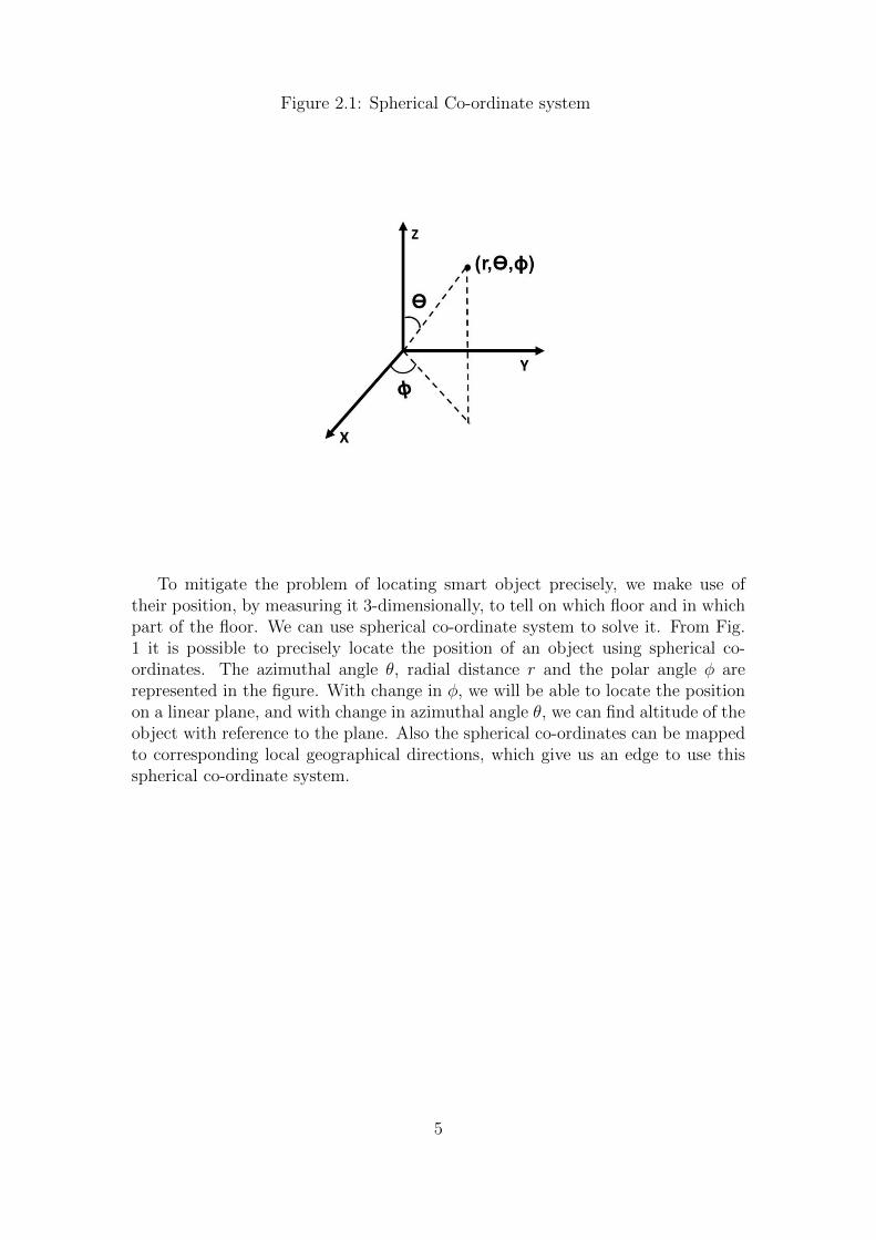
Figure 2.1: Spherical Co-ordinate system

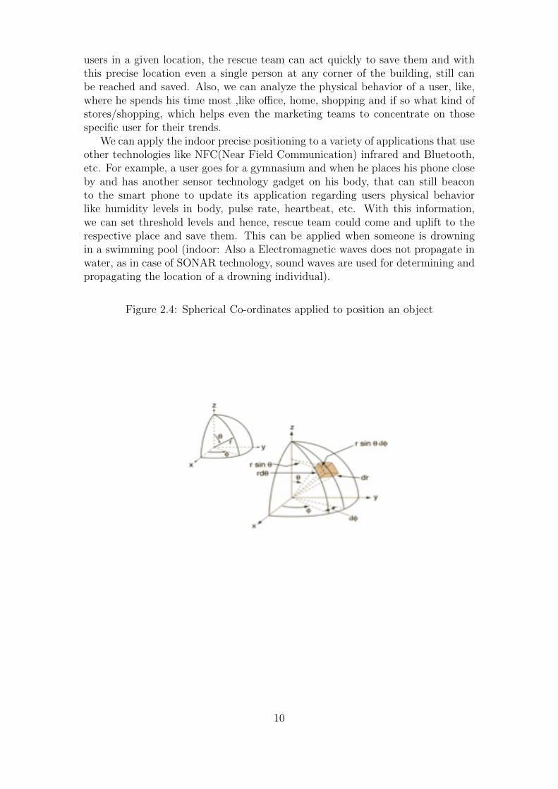
To mitigate the problem of locating smart object precisely, we make use oftheir position, by measuring it 3-dimensionally, to tell on which floor and in whichpart of the floor. We can use spherical co-ordinate system to solve it. From Fig.1 it is possible to precisely locate the position of an object using spherical co-ordinates. The azimuthal angle θ, radial distance r and the polar angle φ arerepresented in the figure. With change in φ, we will be able to locate the positionon a linear plane, and with change in azimuthal angle θ, we can find altitude of theobject with reference to the plane. Also the spherical co-ordinates can be mappedto corresponding local geographical directions, which give us an edge to use thisspherical co-ordinate system.

5

2.2 Related Work

Controneo et al. [5] proposed a naive partition positioning method, wherein thesub region to which a mobile belongs to, is determined based on the signal strengthit receives from an AP. Xu et al. [6] divided the location space into multiple zones.In the positioning phase, they used the maximum likelihood theory to determinethe location of the mobile terminal. Samama et al. [7] pointed out that manyindoor positioning scenarios often do not require high accuracy and it is goodenough to intimate the user some symbolic information, such as which corridoror room the current place is at. In addition, an algorithm is proposed, whichuses 3D symbol positioning. It divides the location space into various positioningsymbolic subspaces and further designed a symbolic subspace resolution to conveythe location information to the user. Gansemer et al. [6] points that the 3Dindoor positioning can be more realistic by RFID(Radio Frequency IdentificationDevices), UWB (Ultra Wide Band) and other technologies. They stressed theneed for 3D indoor positioning using wireless local area networks (WLAN) anda method was proposed that extends isolines algorithm [9], used in 2D WLANindoor positioning to 3D space. Zhong-liang et al. [3] adopted k-means clusteringalgorithm to partition a three dimensional indoor space into multiple regions;namely, location fingerprints with similar Euclidean distance are clustered into oneregion and the central fingerprint of every region is saved. In the positioning phase,the fact that the fingerprint received by the closest mobile terminal estimates thelocation of the mobile terminal. But location information (location of the mobileterminal) is confined to floor, which is strong limitation in this paper. The exactpositioning of a mobile on the floor is not proposed.

2.3 Precise Positioning Algorithm

Our precise positioning algorithm employing the leveling and coning techniquesis proposed in this section. In our algorithm, the precise position of an objectis found by applying horizontal positioning followed by vertical positioning algo-rithms. Throughout this paper, horizontal position is the location of an objectwith respect to the access point and vertical position is the location of an objectwith respect to the base station (as shown in Fig. 2). We use leveling and sec-toring algorithms in finding the horizontal position where as the coning algorithmis applied in case of vertical positioning. The following setup is needed in orderto implement our algorithm. A placement of base station near the building isassumed along with the placement of at least one access point (IEEE 802.11ac ora femto cell or a combination) on each of the floors of the building. It is furtherassumed that, each access point includes an electronically steered unidirectionalantenna, now the horizontal and vertical positioning algorithms are elucidated inthe below sub sections.

6

2.3.1 Horizontal Positioning

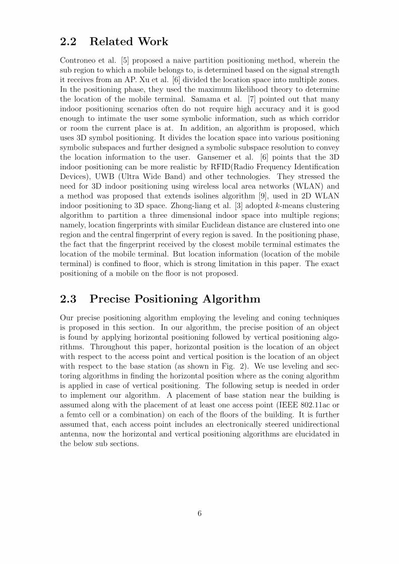
As we discussed before, the horizontal position is calculated with respect to theaccess point situated on each floor of the building. In this paper, the conceptsof leveling and sectoring algorithm [8] are brought into indoor positioning. Thelevels and sectors are formed with respect to the access point to find the horizontalposition. The sectors are segregated with respect to direction of antenna locatedon the access point and the levels are segregated with respect to the power levelsas presented in [8]. The mobile, whose position has to be found out, sends a proberequest to the access point. Based on the RSS levels, the position of the mobilewith respect to access point is determined. This concept is presented in Fig. 3.

Figure 2.2: Leveling and Sectoring in a Horizontal Plane

As shown in Fig. 3, in a horizontal plane, using the access point directionalantenna and power level, we broadcast the beacons. The stations send responsesand based on it the RSS is derived and we can estimate the liner distance fromeach of the access points. Then for each power level in a given sector S1, we havedifferent levels namely L1, L2, L3, etc. The sectors are also formed based on thehorizontal angle and number of sector depend on the φ namely S1, S2, S7, etc.

7

2.3.2 Vertical Positioning

We determine the vertical position using the base station employing the coningtechnique. The azimuthal angle between the antenna and the mobile(situatedon the floor of the building) gives us the vertical position. This brings in theconcept of 3- dimensional sectors and thus the 3D-cone is formed and such conesare packed together in 3-dimensional space and form a sphere. The azimuthalangle is fixed based on the number of floors in a building. To our experiments ourcampus building with 5 floors, hence the vertical rotation is fixed to 60 degreesper step. Since, we have our base station placed at the corner of the building onthe ground floor; we think that a hemi-sphere area of RF finger print coverage in3D would be sufficient to precisely calculate the position. Even in a case of largebuildings or circular shaped buildings, if the base station is placed in the middle,still calculating the position is easy as the second half of the sphere is a mirrorreflection. As shown in Fig. 2, with the help of the base station and the verticalangle or azimuthal angle we know the floor of the building and at the same time,the power leveling done by each access point at each floor would help us the preciselocation of the user in two ways: one is the radial distance from the base stationand the other is the relative distance from the AP per floor. All these APs areconnected in tandem to a localization server, which would use software algorithmto calculate the precise position of the user and the same information is passed tothe user. Let A, B, C be the mobiles whose position has to be found out and BSbe the base station to determine the vertical positioning and AP1, AP2,. . ., AP5be access points to determine the horizontal positioning. Localization Server isemployed to place the data statistics which can further be used to dump data. Wetake the RSS from each user in different power levels and the required distance iscalculated from the obtained RSS.

2.3.3 Machine Learning Techniques into Positioning

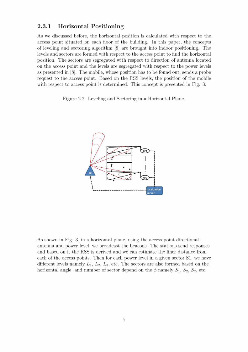
Once we calculate the positions of the users this training data can be fed to a Sup-port Vector Machine (SVM) classifier [1], which gives us a precise finger printingmap, which can be reversed mapped to the dynamic positioning of the object inreal time.

Power level Average RSS Distance

L1 -10 dB 10L2 -30 dB 20L3 -45 dB 40L4 -80 dB 100

Table 2.1: Power leveling with the corresponding RSS levels

In addition, the system can be enhanced, i.e., the formation of sectors, levelsand cones can be more efficient after the training data is fed to the SVM. Com-bining the Fig.2 and Fig.3 for a given access point and Base station(BS) in 3Dgives a sphere and a vertical angle that helps us determined its position.Hence, thelocation of an object can now be precisely located using these levels and sectoring

8

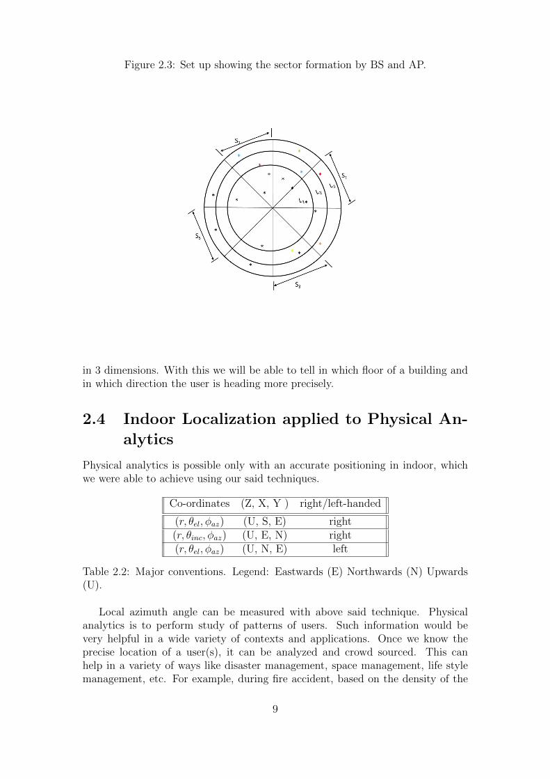
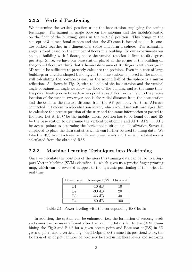
Figure 2.3: Set up showing the sector formation by BS and AP.

in 3 dimensions. With this we will be able to tell in which floor of a building andin which direction the user is heading more precisely.

2.4 Indoor Localization applied to Physical An-

alytics

Physical analytics is possible only with an accurate positioning in indoor, whichwe were able to achieve using our said techniques.

Co-ordinates (Z, X, Y ) right/left-handed

(r, θel, φaz) (U, S, E) right(r, θinc, φaz) (U, E, N) right(r, θel, φaz) (U, N, E) left

Table 2.2: Major conventions. Legend: Eastwards (E) Northwards (N) Upwards(U).

Local azimuth angle can be measured with above said technique. Physicalanalytics is to perform study of patterns of users. Such information would bevery helpful in a wide variety of contexts and applications. Once we know theprecise location of a user(s), it can be analyzed and crowd sourced. This canhelp in a variety of ways like disaster management, space management, life stylemanagement, etc. For example, during fire accident, based on the density of the

9

users in a given location, the rescue team can act quickly to save them and withthis precise location even a single person at any corner of the building, still canbe reached and saved. Also, we can analyze the physical behavior of a user, like,where he spends his time most ,like office, home, shopping and if so what kind ofstores/shopping, which helps even the marketing teams to concentrate on thosespecific user for their trends.

We can apply the indoor precise positioning to a variety of applications that useother technologies like NFC(Near Field Communication) infrared and Bluetooth,etc. For example, a user goes for a gymnasium and when he places his phone closeby and has another sensor technology gadget on his body, that can still beaconto the smart phone to update its application regarding users physical behaviorlike humidity levels in body, pulse rate, heartbeat, etc. With this information,we can set threshold levels and hence, rescue team could come and uplift to therespective place and save them. This can be applied when someone is drowningin a swimming pool (indoor: Also a Electromagnetic waves does not propagate inwater, as in case of SONAR technology, sound waves are used for determining andpropagating the location of a drowning individual).

Figure 2.4: Spherical Co-ordinates applied to position an object

10

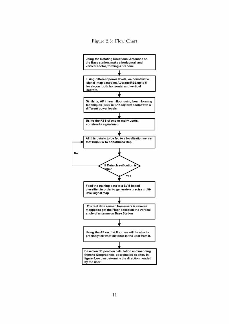
Figure 2.5: Flow Chart

11

2.5 Localization Accuracy

Using GPS in outdoor localization resolution of localization (positioning on earth)can be achieved to certain accuracy. In addition, hop count based localizationmethods rely on power control. Localization up to certain hop count value (froma specified transmitter) leads to certain accuracy depending on the power levelvalue (in homogeneous wireless nodes). But in Indoor Localization using levelingand sectoring/coning, RSS (Received signal Strength) is used as a foot print. Theaccuracy depends on resolution of varying power levels (for leveling) and the beamAngle (of the radiating pattern) of the antenna being steered (in 2D & 3D). Thus3D indoor localization is achieved by quantization of the spherical co-ordinates(r, θ, φ) using power control at the transmitter and steering control (of the an-tenna).

2.6 Application of Proposed Approach for Out-

door Localization

As in the case if Micro/Pico/Femto Base Station, the triangulation procedure canbe utilized using macro cellular base stations as Anchors. Leveling and Sectoringapproach cab be utilized using the macro cellular base stations. Leveling andconing can be utilized for 3D localization of say Helicopters, Fighter air-crafts,civil air-crafts with macro cellular base stations as anchors.

2.7 Improved Accuracy using RCPI

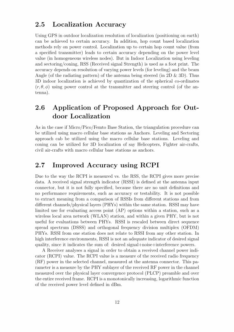
Due to the way the RCPI is measured vs. the RSS, the RCPI gives more precisedata. A received signal strength indicator (RSSI) is defined at the antenna inputconnector, but it is not fully specified, because there are no unit definitions andno performance requirements, such as accuracy or testability. It is not possibleto extract meaning from a comparison of RSSIs from different stations and fromdifferent channels/physical layers (PHYs) within the same station. RSSI may havelimited use for evaluating access point (AP) options within a station, such as awireless local area network (WLAN) station, and within a given PHY, but is notuseful for evaluations between PHYs. RSSI is rescaled between direct sequencespread spectrum (DSSS) and orthogonal frequency division multiplex (OFDM)PHYs. RSSI from one station does not relate to RSSI from any other station. Inhigh interference environments, RSSI is not an adequate indicator of desired signalquality, since it indicates the sum of: desired signal+noise+interference powers.

A Receiver analyses a signal in order to obtain a received channel power indi-cator (RCPI) value. The RCPI value is a measure of the received radio frequency(RF) power in the selected channel, measured at the antenna connector. This pa-rameter is a measure by the PHY sublayer of the received RF power in the channelmeasured over the physical layer convergence protocol (PLCP) preamble and overthe entire received frame. RCPI is a monotonically increasing, logarithmic functionof the received power level defined in dBm.

12

Hence due to its non-reliability due to its non-uniformity between different sta-tions, the accuracy levels are not so precise.Eg: when we measured RSSI betweentwo different chip vendors in the market, one smart phone connect to a particularaccess point at a given position and instant shows -21dBm of RSSI , the other atthe same point and instant showed -17dBm,which is a variation of 5dBm whichleads to a localization error.

2.8 Conclusion

Precise positioning is possible using the spherical coordinates and at a macro level.This technique can also be applied on the base stations. Apart from locating theposition of the users on earth, even flying object above the base station can bedetected using smart antennas, which could aid military applications too. In thenext chapter we deal with reducing the delay in grid based WSN networks. Theyaid in event localization by computing the aggregated data from different clusterheads to a sync/base station within less time.

2.9 References

[1] Krishna Chintalapudi, Anand Padmanabha Iyer, Venkata N. Padmanabhan. Indoor Localization Without the Pain. In Proceedings of the sixteenthannual international conference on Mobile computing and networking, pages12. ACM Press, 2010.

[2] S. Gansemer, S. Hakobyan, S. Puschel, and U. Gromann. 3d WLAN indoorpositioning in multi-storey buildings. In International Workshop on Intelli-gent Data Acquisition and Advanced Computing Systems: Technology andApplications (IDAACS -09), pages 669672, Sep 2009.

[3] D. Zhong-liang and W. Wen-jie and X. Lian-ming. A k-means based methodto identify floor in WLAN indoor positioning system. Computer Engineering& Software, 33(12):114117, 2012.

[4] J. Cheng, Y. Cai, Q. Zhang, J. Cheng, and C. Yan. A new threedimensionalindoor positioning mechanism based on wireless, page 23, Feb 2004.

[5] D. Cotroneo, S. Russo, F. Cornevilli, M. Ficco, and V. Vecchio. Implement-ing positioning services over an ubiquitous infrastructure. In Software Tech-nologies for Future Embedded and Ubiquitous Systems, 2004. Proceedings.Second IEEE Workshop on, pages 1418, May 2004.

[6] F.-Y. Xu and L.-B. Li and Z.-X. Wang. New WLAN indoor localization sys-tem based on distance-loss model with area partition Journal of Electronicsand Information Technology, 30(6):14051408, 2008.

[7] N. Samama. Symbolic 3d wifi indoor positioning system: a deployment andperformance evaluation tool. In Proceedings of the 13th World Congress ofthe International Association of Institutes of Navigation (IAIN -09), page23, Oct 2009.

13

[8] A. Mirza, A. Mohed, and R. Garimella. Energy efficient sectoring basedrouting in wireless sensor networks for delay constrained applications: Amixed approach. In TENCON 2008 - 2008 IEEE Region 10 Conference,pages 16, Nov 2008.

[9] C.-C. Chang and C.-J. Lin. LIBSVM: a library for support vector machines.ACM Transactions on Intelligent Systems and Technology, 3(27), 2011.

[10] U. Gromann and M. Schauch and S. Hakobyan.The accuracy of algorithmsfor WLAN indoor positioning and the standardization

14

Chapter 3

Grid of WirelessSensors:Distributed Computation

3.1 Introduction

Wireless Sensor Networks (WSNs) consist of a set of sensor nodes that are de-ployed in a field and interconnected with a wireless communication network. Eachof these scattered sensor nodes have the capabilities to collect data, fuse androute the data back to the sink/base station (Ian F. Akyildiz, Weilian Su, YogeshSankarasubramaniam & Erdal Cayirci, 2002); (Akyildiz, Weilian, Sankarasubra-maniam, Cayirci, 2001). To collect data, each of these sensor nodes makes decisionbased on its observation of a part of the environment and on partial a-priori in-formation. As larger amount of sensors are deployed in harsher environment, it isimportant that the distributed computation should be robust and fault-tolerant.The identification of an event in a wireless sensor network should be done as fastas possible, thus the computations are done in parallel.

Here we investigate the problem of design of optimal parallel distributed com-putational architecture. In distributed system components located on networkedcomputers communicate and coordinate by passing messages to perform the spec-ified task. Similarly distributed computation is done on distributed nodes con-nected over the network with defined computational model. A model of compu-tation is a formal description of a particular type of computational process. Moredetails about computability theory can be found in the book by (Barry Cooper,2003). This paper assumes the no memory computational model of sensor nodesin the architecture for primitive recursive functions. No memory computationalmodel means the sensor node just has registers to store two values; whenever thesensor node receives any value from the other sensor nodes, it simply computesthe function with its own measured value and the received value and passes theresults to other sensor node(s).

The distributed architecture for WSN needs to be optimal from most of thefollowing points (Rotem, Santoro & Sidney, 1985) :

• Computational complexity

• Transmission delay required for computations

15

• Deployment / Reconfiguration

• Fault Tolerance

The rest of the chapter is as follows: Section II describes the problem state-ment. Section III gives the optimal architecture for primitive recursive functionsand discusses the class of functions, i.e. primitive recursive functions, which canbe solved using grid like architecture and also the fault tolerance capability ofthe proposed architecture. Section IV discusses the network architecture for dis-tributed computation of median. Section V explores the possible applications ofWSNs in transportation system like itinerary planning, dynamic speed boards etc,which makes it user friendly. Finally section VI concludes the paper.

3.2 Distributed Network Architecture for Prim-

itive Recursive Functions

3.2.1 Problem Statement

The problem is to define a globally optimal data structure for calculating the de-fined fusion function over the sensor field. The architecture should be as optimalas possible from the point of view of all the performance measures as discussed inthe above section. The computational model considered is also important whiledefining the suitable distributed architecture. This paper assumes the no mem-ory computational model as discussed before. Thus the problem statement isre-defined; To find the globally optimal architecture, we need to fix some of theperformance measures and try to optimize the other measures. The modified prob-lem statement is:

Given the maximum allowed delay D0, define the globally optimal data struc-ture of the wireless sensor network, for the distributed computation of fusion func-tions of sensed values, in the no memory computational model.

3.2.2 Primitive Recursive Functions

This section discusses the class of functions, i.e. primitive recursive functions,which can be computed optimally on grid like architecture. The basic primi-tive recursive functions are given by these axioms (Piergiorgio Odifreddi & BarryCooper, 2012) :

• Constant function: The 0-ary constant function 0 is primitive recursive.

• Successor function: The 1-ary successor function S, which returns the suc-cessor of its argument, is primitive recursive. That is,

S(k) = k + 1 (3.1)

• Projection function: For every n ≥ 1 and each i with 1 ≤ i ≤ n, the n-aryprojection function P n

i , which returns its ith argument, is primitive recursive.

16

More complex primitive recursive functions can be obtained from the initialfunctions by means of composition and primitive recursion.

• Composition: If g is a function of m arguments h1, h2 . . . hm, where each ofh1, h2 . . . hm is a function of n arguments, then the function f is defined bycomposition from g and h1, h2 . . . hm

f(x1, x2....xm) = g(h1(x1, x2....xm), h2(x1, x2....xm), . . . hm(x1, x2 . . . xm))(3.2)

We write and in the simple case where m = 1 and h1 is designated h, wewrite

f(x) = [goh](x) (3.3)

• Primitive Recursion: A function f is definable by primitive recursion from gand h if:

f(x, 0) = g(x) (3.4)

f(x, s(y)) = h(x, y, f(x, y)) (3.5)

We write f = PR(g, h) when f is definable by primitive recursion from gand h. Here s is the successor function, which when given an argumentn, returns its immediate successor . The primitive recursive functions arethe basic functions and those obtained from the basic functions by applyingthese operations a finite number of times. In WSN domain, simple aggre-gation techniques i.e., maximum, minimum, and average have been used tosave energy while monitoring (Abdelgawad & Bayoumi, 2012). In case ofmore complex fusion functions also, the fusion function can be representedusing primitive recursive function class. Some of the examples of primitiverecursive functions which can be used in fusion are: addition, multiplication,exponentiation, factorial, proper subtraction, defined as “a ≥ b then a−b else0”; Minimum (a1, a2 . . . an), Maximum (a1, a2 . . . an) absolute value, mean,weighted mean, and weighted energy i.e.

a1x21 + a2x

22 + . . .+ anx

2n (3.6)

3.2.3 Grid based Network Architecture

This subsection discusses the optimal distributed architecture for homogeneousand heterogeneous wireless sensor networks. Homogeneous WSN consists of sensornodes with same abilities while heterogeneous WSN consists of sensor nodes withdifferent abilities such as different computing power.

17

Homogeneous WSN

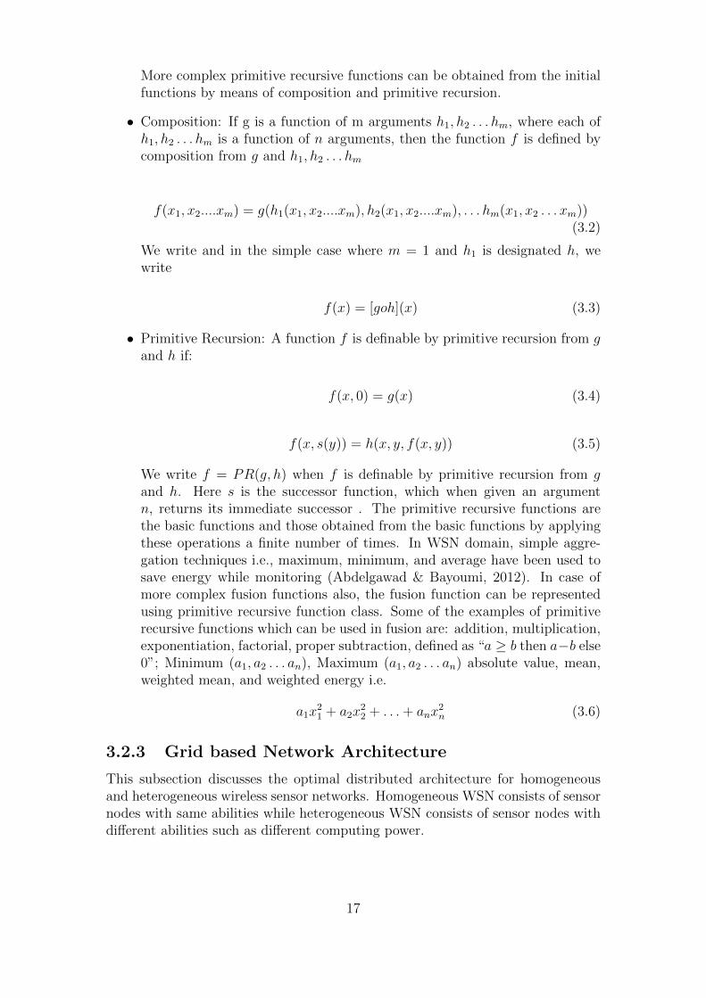
The solution for the above defined problem is a grid like architecture as shown inFig. 3.1

Figure 3.1: Example of a path; from source to destination

In this section, we first discuss the computational complexity of fusion functionslike the minimum/maximum, where only one comparison is needed at every node.Later we show that the same comparisons can be done for other functions as well.

Assume that the total number of processors P is equal to the number of sensornodes in the network.

Calculations are as follows: The number of nodes in each branch is definedas D0, computational complexity in each branch is D0 − 1, total number of suchbranches are N/D0. So, total computational complexity:

= (N/D0)(D0 − 1) +N/D0 + 1

= N − (N/D0) +N/D0 − 1

= N − 1 (3.7)

We can see that the number of comparisons is equal to the minimum compar-isons required for any architecture, which is the lower bound of the computationalcomplexity. This is also possible by a tree kind of architecture. In tree architecturefor maintaining the delay requirement, one node will have multiple child nodes.Also, as any sensor node will receive more number of values simultaneously, more

18

number of registers are needed. Hence, tree kinds of architectures are not suitablein this computational model.

Now let us consider the special class of functions which require x comparisonsat each sensor node. Computational complexity in the case of such functions iscomputed as follows. Computational complexity in each branch is (D0 − 1)x,number of such branches is N/D0 − 1 So, total computational complexity:

= (N/D0)(D0 − 1)x+N/D0 + 1

= Nx− (N/D0)x+ xN/D0 − x

= (N − 1)x (3.8)

Here again the number of comparisons is equal to the minimum required com-parisons. Also this architecture is very suitable for the sensor field from the pointof view of deployment and coverage.

Heterogeneous WSN

Clustering of sensor networks has proved to be very effective in conserving energyin heterogeneous networks. For each cluster, one Cluster Head (CH) is selectedusing the articles (Heinzelman, Chandrakasan & Balakrishnan, 2000); (Younis &Fahmy, 2004). CH is responsible for the collection, fusion and transmission of datafor the cluster, and also, only cluster heads participate in routing other cluster datato the base station/sink. Thus in heterogeneous WSN, we consider three types ofnodes:

• Sensor Nodes

• Cluster Heads

• Base Station/Sink

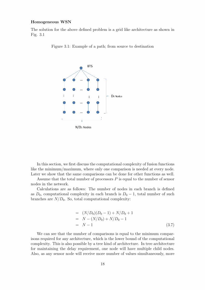
The proposed architecture for this kind of network consists of a hierarchy ofgrid architecture as shown in Fig. 3.2. In the hierarchical grid architecture, eachnode of the final grid architecture is actually a cluster head and this cluster headis connected to other sensor nodes of the cluster using another grid based archi-tecture.

Similarly for more complex networks, multiple hierarchies of clusters can bedone and in such cases multi-hierarchical grid based architecture can be used.

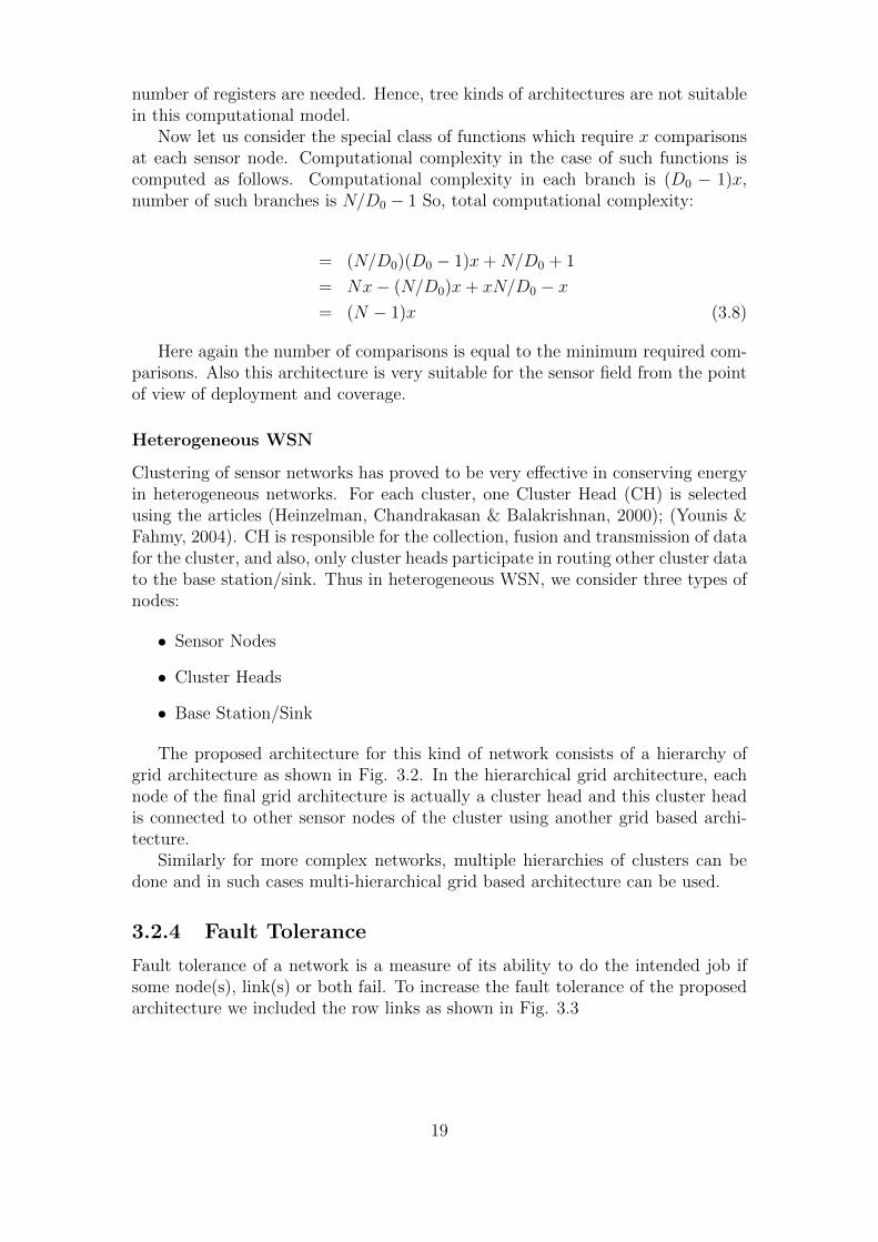
3.2.4 Fault Tolerance

Fault tolerance of a network is a measure of its ability to do the intended job ifsome node(s), link(s) or both fail. To increase the fault tolerance of the proposedarchitecture we included the row links as shown in Fig. 3.3

19

Figure 3.2: Hierarchy of grid architecture

Figure 3.3: Proposed Architecture showing the Row links

20

In this architecture if a node or link goes down, then another path is availableto send the value computed so far, which can be used while calculating the fusionfunction of the other branch. Also identification of error can be done in thisarchitecture. The steps for error detection are as follows:

1. Calculate row wise fusion function

• Calculate the row wise fusion function for each row.

• Calculate the fusion function with each rows calculated value.

2. Similarly calculate column wise fusion function

• Calculate the column wise fusion function for each column.

• Calculate the fusion function with each columns calculated value.

3. If the result of step 1 and 2 are not the same then there is some error in thecomputation.

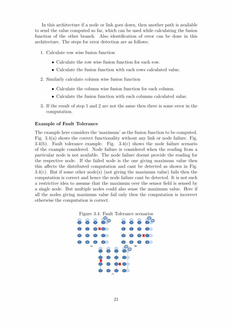
Example of Fault Tolerance

The example here considers the ‘maximum’ as the fusion function to be computed.Fig. 3.4(a) shows the correct functionality without any link or node failure. Fig.3.4(b). Fault tolerance example. Fig. 3.4(c) shows the node failure scenarioof the example considered. Node failure is considered when the reading from aparticular node is not available. The node failure doesnt provide the reading forthe respective node. If the failed node is the one giving maximum value thenthis affects the distributed computation and cant be detected as shown in Fig.3.4(c). But if some other node(s) (not giving the maximum value) fails then thecomputation is correct and hence the node failure cant be detected. It is not sucha restrictive idea to assume that the maximum over the sensor field is sensed bya single node. But multiple nodes could also sense the maximum value. Here ifall the nodes giving maximum value fail only then the computation is incorrectotherwise the computation is correct.

Figure 3.4: Fault Tolerance scenarios

21

From this example it is clear that the one link failure (if the one is passing themaximum value) can be detected in the architecture.

3.2.5 Probability of Error in Maximum Calculation

This subsection calculates the probability of error in grid based architecture formaximum calculation. Let total number of sensor nodes be N . Lets assume nodesfail independently with probability and number of nodes containing the maximumvalue be M . So the probability of error is given by:

Pe =1(NM

)PMf (1 − Pf )(N −M) (3.9)

3.3 Distributed Network Architecture for Me-

dian

3.3.1 Problem Statement

The problem is to find globally optimal architecture for the computation of me-dian.We need to fix some of the performance measures and try to optimize theothers as discussed before. The modified problem statement is: Given the maxi-mum allowed computational complexity O(NlogN), define globally optimal datastructure for the distributed computation of median in a wireless sensor network.

3.3.2 Tree based Network Architecture

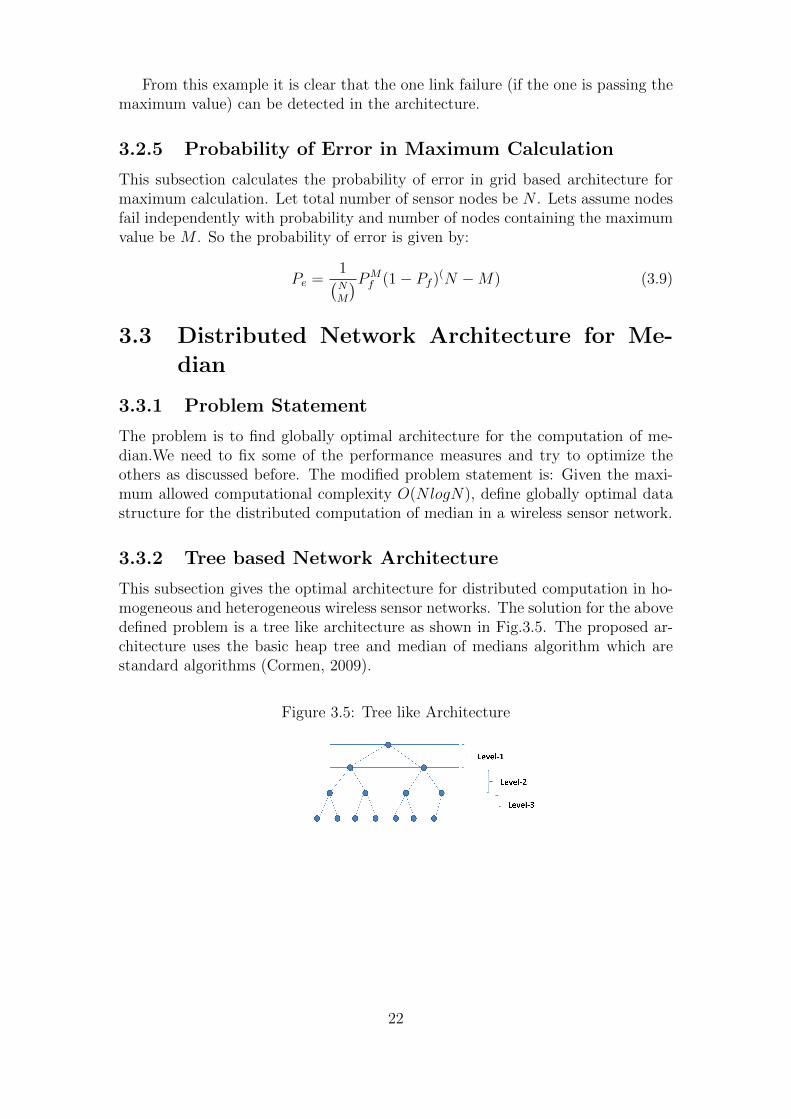
This subsection gives the optimal architecture for distributed computation in ho-mogeneous and heterogeneous wireless sensor networks. The solution for the abovedefined problem is a tree like architecture as shown in Fig.3.5. The proposed ar-chitecture uses the basic heap tree and median of medians algorithm which arestandard algorithms (Cormen, 2009).

Figure 3.5: Tree like Architecture

22

Assumptions

A parent node can communicate with both its left and right child. At each levelin the tree, parallel computation is assumed. Hence D0 is the delay for each level.In the architecture, there is one special node with registers.

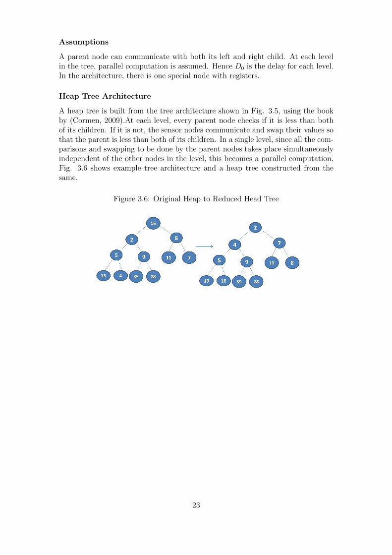
Heap Tree Architecture

A heap tree is built from the tree architecture shown in Fig. 3.5, using the bookby (Cormen, 2009).At each level, every parent node checks if it is less than bothof its children. If it is not, the sensor nodes communicate and swap their values sothat the parent is less than both of its children. In a single level, since all the com-parisons and swapping to be done by the parent nodes takes place simultaneouslyindependent of the other nodes in the level, this becomes a parallel computation.Fig. 3.6 shows example tree architecture and a heap tree constructed from thesame.

Figure 3.6: Original Heap to Reduced Head Tree

23

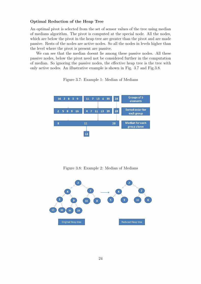
Optimal Reduction of the Heap Tree

An optimal pivot is selected from the set of sensor values of the tree using medianof medians algorithm. The pivot is computed at the special node. All the nodes,which are below the pivot in the heap tree are greater than the pivot and are madepassive. Rests of the nodes are active nodes. So all the nodes in levels higher thanthe level where the pivot is present are passive.

We can see that the median doesnt lie among these passive nodes. All thesepassive nodes, below the pivot need not be considered further in the computationof median. So ignoring the passive nodes, the effective heap tree is the tree withonly active nodes. An illustrative example is shown in Fig. 3.7 and Fig.3.8.

Figure 3.7: Example 1: Median of Medians

Figure 3.8: Example 2: Median of Medians

24

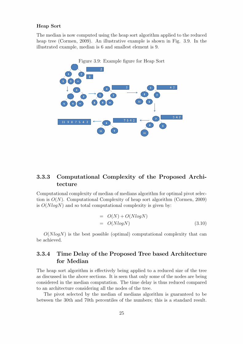
Heap Sort

The median is now computed using the heap sort algorithm applied to the reducedheap tree (Cormen, 2009). An illustrative example is shown in Fig. 3.9. In theillustrated example, median is 6 and smallest element is 9.

Figure 3.9: Example figure for Heap Sort

3.3.3 Computational Complexity of the Proposed Archi-tecture

Computational complexity of median of medians algorithm for optimal pivot selec-tion is O(N). Computational Complexity of heap sort algorithm (Cormen, 2009)is O(NlogN) and so total computational complexity is given by:

= O(N) +O(NlogN)

= O(NlogN) (3.10)

O(NlogN) is the best possible (optimal) computational complexity that canbe achieved.

3.3.4 Time Delay of the Proposed Tree based Architecturefor Median

The heap sort algorithm is effectively being applied to a reduced size of the treeas discussed in the above sections. It is seen that only some of the nodes are beingconsidered in the median computation. The time delay is thus reduced comparedto an architecture considering all the nodes of the tree.

The pivot selected by the median of medians algorithm is guaranteed to bebetween the 30th and 70th percentiles of the numbers; this is a standard result.

25

Thus the heap tree reduces by a decent proportion, i.e. at least 30% and at most70%. Hence the proposed architecture works well in reducing the delay by a decentextent.

This architecture uses a combination of median of medians and min heap al-gorithm resulting in worst case computational complexity of and reduced timedelay.

3.4 Applications

This section discusses the extension of WSNs to exploit its applications in trans-portation system. The Internet of Things (IoT) technology will revolutionize lifeas we know it. WSNs act as a key enabling technology for IoT to come into real-ity. IoT along with Vehicular Ad-Hoc networks (VANETs) can be used to makethe transportation system user-friendly and hassle free. This section presents theapplications in transportation system that can revolutionize life of the users. Thetraffic problems can be suitably solved as graph problems i.e. using graph theory(Darshankumar Dave & Nityangini Jhala, 2014); (Baruah, 2014). The follow-ing applications can involve the use of current technologies like IoT, GPS, andVANETs etc.

3.4.1 Dynamic Speed Boards

As of today, we do not have dynamic speed boards available but only static speedboards. The aim of this application is to update the speed boards regularly i.e.every 15minutes. For this we need an estimate of the traffic flow in the routes,which can be estimated using the article by (Baruah, 2014). The complete trafficinformation of a network can be obtained and using this, the nominal speed in agiven route which can be safe for a vehicle to travel with, can be estimated as perthe traffic congestion information available in the particular route (Baruah, 2014).

This nominal speed is displayed on the speed board in that route. The trafficflow information obtained using (Baruah, 2014) can be obtained every 15minutesso that the speed estimate can be updated regularly on the speed boards.

Speed limit indications at school zones can be based on school timings i.e.dynamic variation in the speed board limits in the morning during school openingand in the evening during school closing can be done. A special case will beconsidered in the following sub-section.

In case an accident occurs on a highway, it would be better to indicate a lowerspeed on the speed board in a route which leads to that particular route in whichthe accident has happened so that the user does not have to wait near the placewhere the accident has happened. Instead if he slows down before reaching thatroute itself, by the time he reaches the place of accident, the place may be clearedof traffic/crowd. This particular speed, at which a user must drive so that bythe time he reaches the place of accident the traffic clears off, can be estimatedby knowing the time of clearance. This time of clearance can be estimated using(Jiang, Ming, Chung & Yang beibei, 2014).

26

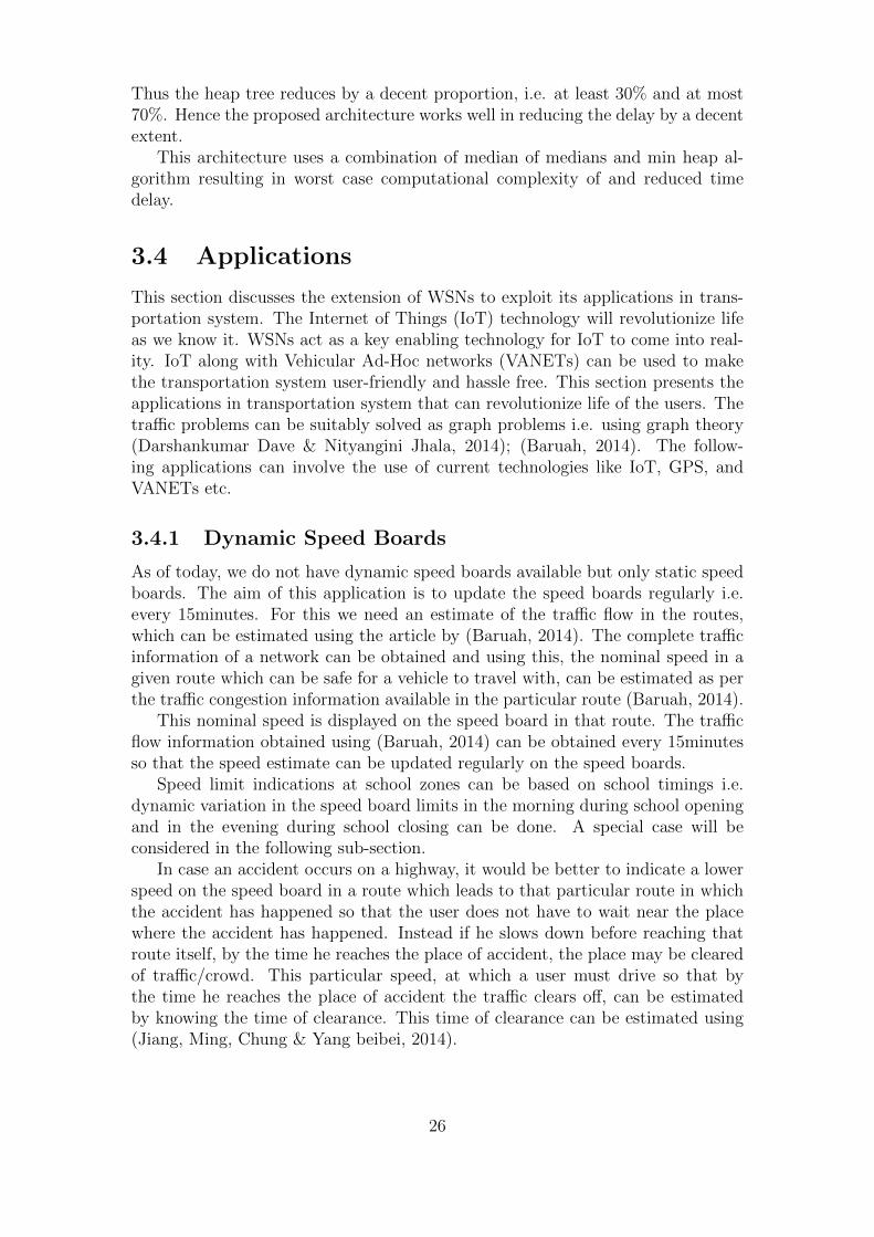
3.4.2 Dynamic Time Estimate

The aim of this application is to give a dynamic time estimate i.e. the approximatetime that a vehicle can take from a selected source to a selected destination as perthe traffic flow present at that particular time. From the above sub-section, wehave an estimate of the average speed of a vehicle in every route. The exampleillustrated in Fig. 3.10 explains how the time estimate from a source to destinationis obtained.

Figure 3.10: Dynamic Time Estimate

In Fig. 3.10, let the source be A and the destination be C. If the route coversvertices 1, 2 and B from source to destination, the path becomes A-1-2-B-C. Thetime estimate from A to C would be

d(A, 1)

v(A, 1)+d(1, 2)

v(1, 2)+d(2, B)

v(2, B)+d(B,C)

v(B,C)(3.11)

d(a, c) is the distance from a to c; v(a, c) is the speed estimate obtained inthe a − c route from the above subsection as per the traffic congestion at thatparticular time. As soon as a particular source and destination are selected, thiskind of calculation is done and the time estimate is displayed for the user. Ifmultiple paths from a source to a destination through different via-routes areavailable, the time estimate in every path is displayed similarly, for the user tochoose a route as per his convenience; for example, the minimum time estimateone i.e. the route which takes shortest time to reach the destination.

Time estimate from a source to destination is already available on Google Maps,but it is not a dynamic one while the time estimate calculated here is dynamic.It is made dynamic as the speed estimate used is a dynamic one i.e. the nominalspeed in the routes is estimated regularly as discussed before.

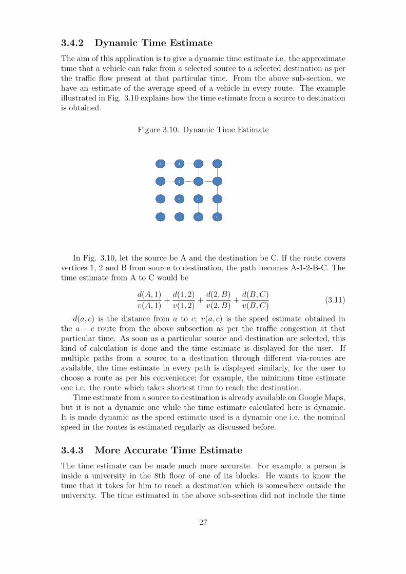
3.4.3 More Accurate Time Estimate

The time estimate can be made much more accurate. For example, a person isinside a university in the 8th floor of one of its blocks. He wants to know thetime that it takes for him to reach a destination which is somewhere outside theuniversity. The time estimated in the above sub-section did not include the time

27

taken for him to come down to the ground floor of the block. Even this time canbe included in the time estimate as follows. The latitude, longitude and altitude ofhis position in the 8th floor and the nearest GPS location of a place in the groundfloor or just outside the block/building that he is in, can be known (Pillalamarri,Murthy, 2015). Considering an average speed of the person, we can calculate thetime it takes for him to reach the ground floor of the building. This time addedto the time estimate calculated in the above sub-section makes it more accurate.An example is illustrated in Fig. 3.11.

Figure 3.11: More Accurate Time Estimate

In the example considered, the person is in the 8th floor of a building and hewants to reach the destination place C. The latitude, longitude and altitude of hisposition in 8 th floor i.e. at node ‘8’ and that at node ‘0’ which is the groundfloor of the building can be known Pillalamarri, Murthy, 2015). By calculating thedifference in both the altitudes and dividing it by the average speed of a person,we get the time taken for him to reach ‘0’ from ‘8’. Now from ‘0’ to reach place‘C’, the time taken for the path 0-A-B-C can be calculated as discussed before.Theaccuracy is increased by including the path from 8 to 0, where previously the pathfor the time estimate included only ‘0’ to ‘C’.

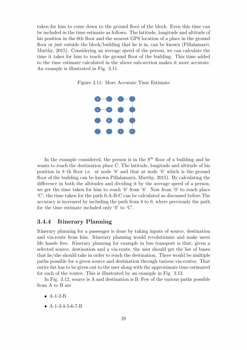
3.4.4 Itinerary Planning

Itinerary planning for a passenger is done by taking inputs of source, destinationand via-route from him. Itinerary planning would revolutionize and make userslife hassle free. Itinerary planning for example in bus transport is that; given aselected source, destination and a via-route, the user should get the list of busesthat he/she should take in order to reach the destination. There would be multiplepaths possible for a given source and destination through various via-routes. Thatentire list has to be given out to the user along with the approximate time estimatedfor each of the routes. This is illustrated by an example in Fig. 3.12.

In Fig. 3.12, source is A and destination is B. Few of the various paths possiblefrom A to B are

• A-1-2-B

• A-1-3-4-5-6-7-B

28

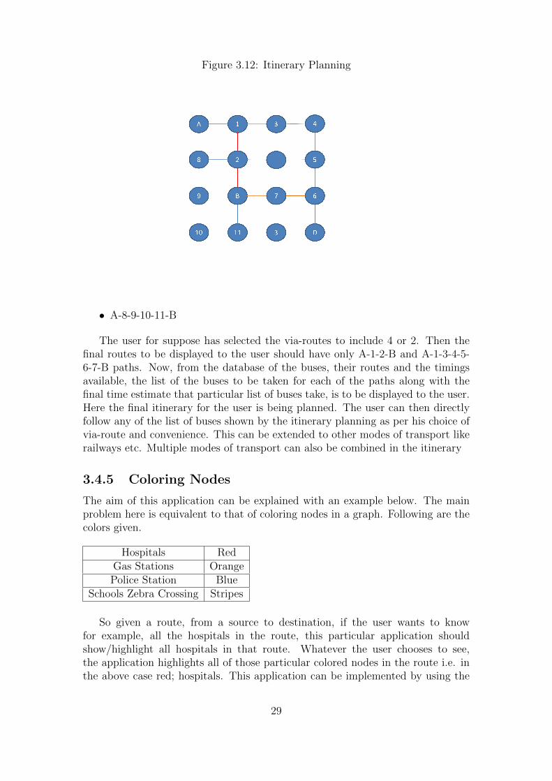
Figure 3.12: Itinerary Planning

• A-8-9-10-11-B

The user for suppose has selected the via-routes to include 4 or 2. Then thefinal routes to be displayed to the user should have only A-1-2-B and A-1-3-4-5-6-7-B paths. Now, from the database of the buses, their routes and the timingsavailable, the list of the buses to be taken for each of the paths along with thefinal time estimate that particular list of buses take, is to be displayed to the user.Here the final itinerary for the user is being planned. The user can then directlyfollow any of the list of buses shown by the itinerary planning as per his choice ofvia-route and convenience. This can be extended to other modes of transport likerailways etc. Multiple modes of transport can also be combined in the itinerary

3.4.5 Coloring Nodes

The aim of this application can be explained with an example below. The mainproblem here is equivalent to that of coloring nodes in a graph. Following are thecolors given.

Hospitals RedGas Stations OrangePolice Station Blue

Schools Zebra Crossing Stripes

So given a route, from a source to destination, if the user wants to knowfor example, all the hospitals in the route, this particular application shouldshow/highlight all hospitals in that route. Whatever the user chooses to see,the application highlights all of those particular colored nodes in the route i.e. inthe above case red; hospitals. This application can be implemented by using the

29

very recent technique of identifying buildings with zippr code, invented by AdityaVuchi. Every building has got a unique zippr code.

Every location on the earth has got a latitude, longitude and altitude associ-ated with it and they can be found with the present technology of Google Maps.The latitude, longitude and altitude of both the source and destination can befound using this. We then obtain the zippr codes of all buildings with their lati-tude and longitude lying in the range between those of the source and destination;equivalently we are obtaining all the buildings which lie between the source anddestination. According to the zippr code of the buildings obtained, we can identifythe buildings as restaurant/hospital/school/police station etc, as most probablythe zippr code assigned to a building would be dependent on the type of buildingthat it is, while registration. Once we get the zippr code of a building, the zipprapplication itself gives us the route from our present location then to the build-ing. This makes life easier to search for schools/hospitals/police stations etc, in aparticular route. For this application to come into reality the use of zippr codesfor buildings has to increase; this may take time.

3.4.6 Possible Improvements in Google Maps

• Traffic patterns as of today, are given from 8am to 8pm which can be im-proved to make it 24/7.

• Time estimates from a source to destination can be made dynamic.

• The applications given in the above sub-sections can be included in theGoogle Maps.

3.5 Conclusion

This chapter discusses the optimal architecture for distributed computation inwire- less sensor networks. Computational complexity for a fixed maximum al-lowed delay is calculated, which shows that this architecture is the solution forthe given computational model. It is also shown that the proposed architecture isvery efficient with respect to faults in the network. An optimal architecture for dis-tributed computation of median, with reduced time delay and optimal worst casecomputational complexity is discussed. The applications of WSN like, itineraryplanning that can revolutionize the present transportation system are presented.In the next chapter, we discussed how we can reduce the transmission delay in gridbased architecture which aid us in localizing an event (ex: temperature recordedor any such similar parameters).

30

3.6 References

[1] Akyildiz, I. F., Su, W., Sankarasubramaniam, Y., & Cayirci, E. (2002). Asurvey on sensor networks. Communications magazine, IEEE, 40(8), 102-114.

[2] Akyildiz, I. F., Su, W., Sankarasubramaniam, Y., & Cayirci, E. (2002).Wireless sensor networks: a survey. Computer networks, 38(4), 393-422.

[3] Cooper, B. S. (2003). Computability Theory. Chapman Hall/Crc Mathe-matics Series.

[4] Rotem, D., Santoro, N., & Sidney, J. B. (1985). Distributed sorting. IEEETransactions on Computers, 34(4), 372-376.

[5] Odifreddi, P., & Cooper, S. B. (2005). Recursive functions.

[6] Abdelgawad, A., & Bayoumi, M. (2012). ResourceAware data fusion algo-rithms for wireless sensor networks (Vol. 118). Springer Science & BusinessMedia.

[7] Heinzelman, W. R., Chandrakasan, A., & Balakrishnan, H. (2000, January).Energy-efficient communication protocol for wireless microsensor networks.In System sciences, 2000. Proceedings of the 33rd annual Hawaii interna-tional conference on (pp. 10-pp). IEEE.

[8] Younis, O., & Fahmy, S. (2004). HEED: a hybrid, energy-efficient, dis-tributed clustering approach for ad hoc sensor networks. Mobile Computing,IEEE Transactions on, 3(4), 366-379.

[9] Cormen, T. H. (2009). Introduction to algorithms. MIT press.

[10] https://en.wikipedia.org/wiki/Median of medians [Active as on 12-04-2016]

[11] Darshankumar Dave, & Nityangini Jhala. (2014). Application of GraphTheory in Traffic Management. International Journal of Engineering andInnovative Technology, 3(12).

[12] Baruah, A. K. (2014). Traffic Control Problems using Graph Connectivity.International Journal of Computer Applications, 86(11).

[13] Jiang, R., Qu, M., & Chung, E. (2014). Traffic incident clearance time andarrival time prediction based on hazard models. Mathematical Problems inEngineering, 2014.

[14] Pillalamarri, B., & Murthy, G. R. (2015, April). Precise positioning in 3Dusing spherical co-ordinates as applied to indoor localization. In Communi-cation Technologies (GCCT), 2015 Global Conference on (pp. 8-11). IEEE.

[15] http://www.dnaindia.com/india/report-zippr-a-new-appthat-shortens-your-address-1982794 [Active as on 12- 04-2016]

31

Chapter 4

Outdoor Navigation: EfficientOrder Statistics computation

4.1 Introduction

Wireless sensor networks (WSNs) are widely employed to perform distributed sens-ing in various fields. The sensing is done in order to have a better understanding ofthe monitored entity.WSNs provide a bridge between the real physical and virtualworlds. Recent advances in wireless communications and electronics have enabledthe development of low power, low cost, multifunctional sensor distances. Each ofthese scattered sensor nodes have the capabilities to collect data, fuse data androute the data back tothe sink/base station. To collect data, each of these sensornodes makes decision based on its observation of a part of the environment and onpartial a-priori information. Each sensor node simply computes the fusion func-tion with its own measured value and the received value and passes the results tothe other sensor node(s).The identification of event in a wireless sensor networkshould be done as fast as possible, thus the computations are done in parallel.

In purview of such efficient individual sensor nodes, we will consider few deeperproblems that can be addressed in WSNs. This paper assumes each of the sensornodes to have self-configurable and data processing ability. The network archi-tectures discussed in this paper are capable of collecting, routing and fusing thedata. This paper is an extension of our previous paper [1], giving solutions toa few deeper problems and exploiting the grid based architecture to increase theefficacy of the computation in regards to various aspects.

The rest of the paper is organized as follows: Section II addresses the localiza-tion problem in WSNs. The optimal computation of order statistics is discussedin Section III. Section IV discusses the efficient grid based architecture, whichaddresses the challenge of reducing the transmission delay. Section V describesthe temporal aspect in computing the statistics in WSNs. Finally, Section VIconcludes the paper.

32

4.2 Localization

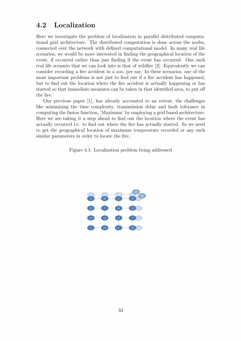
Here we investigate the problem of localization in parallel distributed computa-tional grid architecture. The distributed computation is done across the nodes,connected over the network with defined computational model. In many real lifescenarios, we would be more interested in finding the geographical location of theevent, if occurred rather than just finding if the event has occurred. One suchreal life scenario that we can look into is that of wildfire [2]. Equivalently we canconsider recording a fire accident in a zoo, per say. In these scenarios, one of themost important problems is not just to find out if a fire accident has happened,but to find out the location where the fire accident is actually happening or hasstarted so that immediate measures can be taken in that identified area, to put offthe fire.

Our previous paper [1], has already accounted to an extent, the challengeslike minimizing the time complexity, transmission delay and fault tolerance incomputing the fusion function, ‘Maximum’ by employing a grid based architecture.Here we are taking it a step ahead to find out the location where the event hasactually occurred i.e. to find out where the fire has actually started. So we needto get the geographical location of maximum temperature recorded or any suchsimilar parameters in order to locate the fire.

Figure 4.1: Localization problem being addressed

33

Firstly both row wise and column wise fusion functions [1] i.e. here ‘Maximum’are obtained. The steps to localize the event are as follows:

• Compute the maximum of all the obtained row wise maximums

• Compute the row from which this maximum is obtained. This is the row inwhich the maximum of the grid is lying.

• Compute the maximum of all the obtained column wise maximums

• Compute the column from which this maximum is obtained. This is thecolumn in which the maximum of the grid is lying.

From this, the row and column of the maximum in the grid are obtained andhence the maximum is localized i.e. as per the example of wildfire, the geographicallocation of the maximum temperature is obtained; the location where the fireactually started (or) is happening is identified. Following the above steps for thegrid architecture shown in Fig 4.1, location of the maximum is 2nd row 3rd columnand value of the maximum is 29.

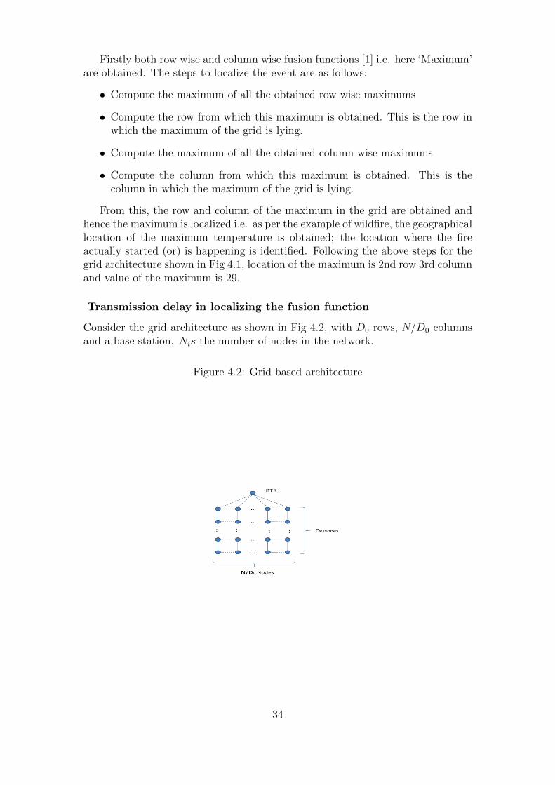
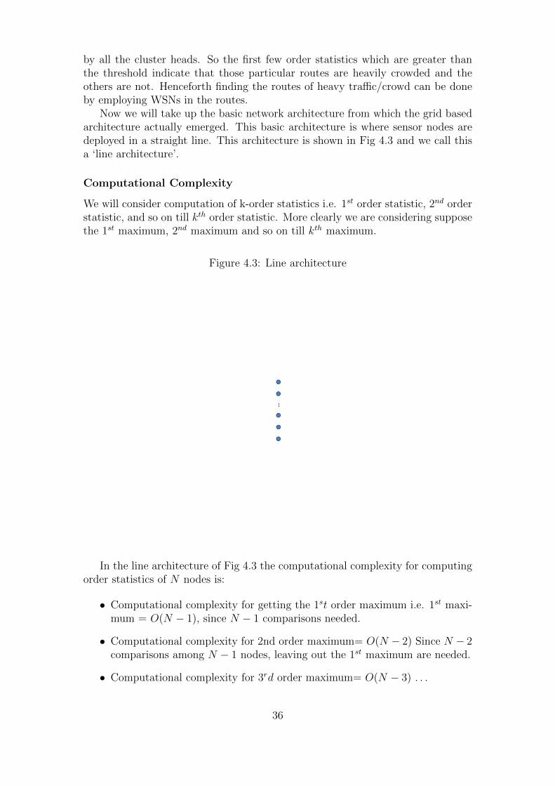
Transmission delay in localizing the fusion function

Consider the grid architecture as shown in Fig 4.2, with D0 rows, N/D0 columnsand a base station. Nis the number of nodes in the network.

Figure 4.2: Grid based architecture

34

Let the transmission delay between two neighboring nodes= 1.

1. Transmission delay in computing all row wise maximums is ((N)//D0) − 1

2. Transmission delay in computing all the column wise maximums is D0 − 1

3. Transmission delay in obtaining the maximum of all the row wise maximumsis D0 − 1.

4. Transmission delay in obtaining the maximum of all the column wise maxi-mums is (N/(D0) − 1).

5. Total transmission delay in localizing the ‘Maximum’ of the grid is 2(N/D0+D0 − 2).

This is the case when the considered grid architecture is fault tolerant. Thechallenge of incorporating fault tolerance in the architecture has already beenaddressed in our previous paper [1].

Computational Complexity

Computational complexity of the grid-based architecture for computing maximum[1] is O(N) .Hereby we have the grid based architecture for computation of max-imum, with optimal computational complexity of O(N) along with incorporatingthe localization problem.

4.3 Order Statistics

In this section we will take up dealing with real life scenarios which need thecomputation of order statistics. In statistics, order statistics refers to the leastor largest order statistic i.e. the least or largest of a statistical sample. We willtake up one such real life scenario which needs computation of order statistics.For example given a colony with many road routes between any two places, whichis usually the case; we want to find out the routes which are filled with heavytraffic/crowd so that people can avoid these routes to a place and can take up aroute which is less crowded. In order to automate this, we deploy efficient sensornodes heavily in every route of the colony. In every route, a cluster head is chosenfrom the set of sensor nodes of that route. All these cluster heads can be seenas forming another sensor network. A threshold for the traffic/crowd is fixedwhich if crossed, people are signaled about that particular route being crowded/ofheavy traffic so that they can skip that route. Moreover in this example, we areinterested in computing only a few order statistics which are greater than or equalto the decided threshold i.e. we are interested in computing the 1st maximum, 2nd

maximum, 3rd maximum and so on till kth maximum.A fusion function is computed in every route, which depicts the parameters like

congestion in the route, based on which one can decide if the route is crowded. Thecluster head in every route gets the ‘Maximum’ value of the parameters consideredfor sensing the crowd/traffic. The sensor network formed by all the cluster heads ofthe routes now computes the order statistics of the sample of maximums computed

35

by all the cluster heads. So the first few order statistics which are greater thanthe threshold indicate that those particular routes are heavily crowded and theothers are not. Henceforth finding the routes of heavy traffic/crowd can be doneby employing WSNs in the routes.

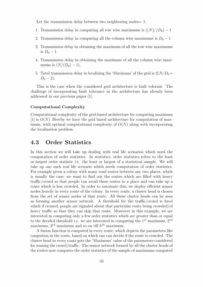
Now we will take up the basic network architecture from which the grid basedarchitecture actually emerged. This basic architecture is where sensor nodes aredeployed in a straight line. This architecture is shown in Fig 4.3 and we call thisa ‘line architecture’.

Computational Complexity

We will consider computation of k-order statistics i.e. 1st order statistic, 2nd orderstatistic, and so on till kth order statistic. More clearly we are considering supposethe 1st maximum, 2nd maximum and so on till kth maximum.

Figure 4.3: Line architecture

In the line architecture of Fig 4.3 the computational complexity for computingorder statistics of N nodes is:

• Computational complexity for getting the 1st order maximum i.e. 1st maxi-mum = O(N − 1), since N − 1 comparisons needed.

• Computational complexity for 2nd order maximum= O(N − 2) Since N − 2comparisons among N − 1 nodes, leaving out the 1st maximum are needed.

• Computational complexity for 3rd order maximum= O(N − 3) . . .

36

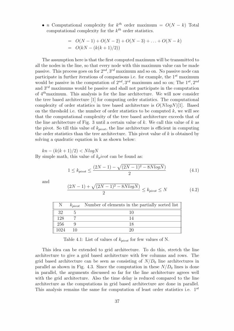
• n Computational complexity for kth order maximum = O(N − k) Totalcomputational complexity for the kth order statistics.

= O(N − 1) +O(N − 2) +O(N − 3) + . . .+O(N − k)

= O(kN − (k(k + 1)/2))

The assumption here is that the first computed maximum will be transmitted toall the nodes in the line, so that every node with this maximum value can be madepassive. This process goes on for 2nd, 3rd maximum and so on. No passive node canparticipate in further iterations of comparisons i.e. for example, the 1st maximumwould be passive in the computation of 2nd, 3rd maximum and so on; The 1st, 2nd

and 3rd maximums would be passive and shall not participate in the computationof 4thmaximum. This analysis is for the line architecture. We will now considerthe tree based architecture [1] for computing order statistics. The computationalcomplexity of order statistics in tree based architecture is O(NlogN)[1]. Basedon the threshold i.e. the number of order statistics to be computed k, we will seethat the computational complexity of the tree based architecture exceeds that ofthe line architecture of Fig. 3 until a certain value of k. We call this value of k asthe pivot. So till this value of kpivot, the line architecture is efficient in computingthe order statistics than the tree architecture. This pivot value of k is obtained bysolving a quadratic equation in k as shown below:

kn− (k(k + 1)/2) < NlogNBy simple math, this value of kpivot can be found as:

1 ≤ kpivot ≤(2N − 1) −

√(2N − 1)2 − 8NlogN)

2(4.1)

and(2N − 1) +

√(2N − 1)2 − 8NlogN)

2≤ kpivot ≤ N (4.2)

N kpivot Number of elements in the partially sorted list

32 5 10128 7 14256 9 181024 10 20

Table 4.1: List of values of kpivot for few values of N.

This idea can be extended to grid architecture. To do this, stretch the linearchitecture to give a grid based architecture with few columns and rows. Thegrid based architecture can be seen as consisting of N/D0 line architectures inparallel as shown in Fig. 4.3. Since the computation in these N/D0 lines is donein parallel, the arguments discussed so far for the line architecture agrees wellwith the grid architecture. Also the time delay is reduced compared to the linearchitecture as the computations in grid based architecture are done in parallel.This analysis remains the same for computation of least order statistics i.e. 1st

37

minimum, 2nd minimum and so on till kth minimum since computing the minimumis also a matter of comparison of neighboring sensor values.

Furthermore this approach has a gain factor of 2; since with the computedvalue of kpivot, computation of both ‘first kpivot maximums’ and the ‘first kpivotminimums’ are made efficient by the line architecture as compared to that by thetree architecture. As a result we arrive at the partial sorted list of the sensor valuesby computing the first kpivot minimums and maximums as indicated in Table I. Ina way, we have exploited the grid based architecture in getting the partial sortedlist.

4.4 Efficient Computation In Grid Based Archi-

tecture

We can exploit the grid based architecture furthermore to reduce the transmissiondelay in computing the order statistics. Consider the grid architecture shown inFig. 4.2. In every column of the grid, to compute the maximum of the values inthe column, the generic method is to compare every two neighboring sensor valuesstarting from the top/bottom. This computation is parallel i.e. the comparisonsin each of the columns happen independent of the other columns. So the grid canbe treated as a set of few line architectures put together and connected. In eachof the line architectures, the steps shown below are followed.

1. Simultaneously start comparing from the top and bottom. We call the com-parisons started from the top as forward pass and that from the bottom asbackward pass.

2. Somewhere near the middle of the line, we get two sensor values; one is themaximum of all the sensor values lying above in the line i.e. the maximumobtained from the forward pass; the other is the maximum of all the sensorvalues lying below in the line i.e. maximum obtained from the backwardpass.

3. The maximum of these two values gives the maximum of the line architecture.

4. Since the computation is done in parallel, we will now have a set of maximumsobtained from all the columns.

5. Equivalently we have one line architecture formed, filled with the maximumscomputed from every column of the grid.

6. The forward and backward pass in this line architecture gives the maximumvalue of the complete grid architecture.

This analysis applies equally well in the computation of order statistics i.e. leastorder statistics and largest order statistics. Transmission delay in computing themaximum:

Let the transmission delay in comparing two neighboring values = 1. In theusual method of computation of maximum in a grid architecture [1]:

38

1. Delay in computing the maximum in columns of the grid= D0 − 1

2. Delay in computing the Maximum of all maximums obtained from each ofthe columns = ((N)(D0)−1).So Total transmission delay= (D0+N/D0−2).

Transmission delay obtained using the forward and backward passes method:

1. Delay in computing the maximum in columns of the grid = (D0/2)) if D0 iseven; else (D0 + 1)/2

2. Delay in computing the Maximum of all maximums obtained from each ofthe columns = (N/D0)/2 if ND0 is even; else ((N(D0)) + 1)/2

3. So total transmission delay is the sum of the above two terms which variesdepending on if D0 is even or odd, but in both the cases the delay is if theorder of (D0 +N/D0)/2

We can clearly see that the transmission delay is almost halved as comparedto that obtained with the usual method [1] in grid architecture. This idea can beextended to the computation of order statistics and primitive recursive functions[1] in grid architecture.

4.5 Temporal Statistics

Till now we have been looking at the computation of spatial statistics i.e. com-putation of fusion function over space; fusion function of sensed values over thedeployed network architecture. There was no temporal aspect considered. We willnow consider the temporal aspect being incorporated in computing statistics innetwork architectures. In addition to spatial statistics, computation of temporalstatistics may also be important in real life scenarios. For example, if one is in-terested in finding out the variation of temperature of a place. Employing anyof the architectures discussed till now, one can find the specific fusion function,both temporally and spatially. This can be made possible if the temporally sensedvalues are recorded by each of the sensor nodes so that the fusion function can becomputed by each of the sensor nodes, with these temporally recorded values. Forexample, we will see the temporal computation of maximum. In the traffic flowdetection example taken above, we will consider finding the temporal variations inthe traffic flow i.e. how the traffic flow is varying over time.

The fusion function i.e. here maximum, computed in every route is sent to thecluster head of that route. At the cluster heads, the received maximum is recordedand saved at regular intervals, while the spatial computation of maximum is doneover the sensor values of all the cluster heads. Suppose we want to see the variationof traffic flow separately in every route in a single day. The cluster heads recordthe received maximum from their nodes, for every 3hours. After 24 hours, each ofthe cluster heads will have 8 values of temporal maximums. For every cluster head,these 8 maxima indicate the variation of traffic flow, in that particular route. Atevery cluster head, the maximum of the recorded 8 values can be found out thereby

39

computing the temporal maximum. This way the temporal maximum in everyroute can be computed along with the spatial maximum. This temporal aspectcan be very well extended to the computation of primitive recursive functions.

4.6 Conclusion

In this chapter, we exploited the grid and tree based network architectures in thecomputation of fusion functions to extract the maximum possible statistics. Lo-calization problem is addressed in Section 4.2 and it is shown that localizationin grid based architecture can be achieved, that can be employed in real life sce-narios. Importance of the efficient computation of order statistics is discussed inSection 4.3. Section 4.4 showed that the transmission delay in grid based archi-tecture for computation of maximum can be reduced to almost half that can beextended to primitive recursive functions. Section4.5 discussed the temporal as-pect in computing fusion functions which can be efficiently employed in real lifescenarios.

4.7 References

[1] Devanaboyina, T., Pillalamarri, B., & Garimella, R. M. (2015). DistributedComputation in Wireless Sensor Networks: Efficient Network Architecturesand Applications in WSNs. International Journal of Wireless Networks andBroadband Technologies (IJWNBT), 4(3), 14-32.

[2] https://en.wikipedia.org/wiki/Wildfire [Active as on 18-06-2016]

40

Chapter 5

Conclusion and Future work

5.1 Conclusion

Any application that would depend on indoor positioning shall need an exactlocation. Our aim is to find the exact geographical location of the user/event, toaid those applications. Precise indoor localization aided with our above mentionedtechniques help in different ways. That also include physical analytics to analyzethe study of patterns of users. Such information would be very helpful in a widevariety of contexts and for different applications. If precise location of a user(s),can be analyzed and crowd sourced, it can help in a variety of ways like disaster,space, life style management, etc.

Our proposed techniques (Chapter 3 and Chapter 4) will enhance and improvethe accurate positioning, while minimizing the computational delay and localiza-tion of events in WSNs. Many challenges that emerging applications face in usingphysical analytics can be overcome via accurate localization.

Using our work with respect to computational complexity, delay of transmis-sion,it gives freedom to select which architecture suits better for a given applica-tion.

This work on 3D localization and Wireless Sensor Networks can potentiallyimprove many applications when used in tandem or can be applied individuallybased on the application requirements.

5.2 Future Work

Our work could be further extended to experiments and the algorithms used inthis thesis can be tested using simulation study. With the emergence of Internetof Things (IoT), this work could be applied in IoT based devices to improve theperformance of the indoor/outdoor localizations. As architecture of the WSNsshall play a vital role, in deciding different parameters of intrest based on anapplication in the context,one can think of hybrid architectures and experimentour proposed computational complexity and Delay of transmission.

41

Related publicationsJournals

1. Balakrishna Pillalamarri, G. R. Murthy, “Improved Precise Positioningin 3D Using RCPI and Spherical Co-ordinates as Applied to Indoor Local-ization”, Journal of Multidisciplinary Engineering Science and Technology(JMEST)

2. T. Devanaboyina, Balakrishna Pillalamarri, G. R. Murthy, “DistributedComputation in Wireless Sensor Networks”, International Journal of Wire-less Networks and Broadband Technologies (IJWNBT)

3. T. Devanaboyina, Balakrishna Pillalamarri, G. R. Murthy, “Efficient Or-der Statistics : Routing,Fusion and Localization in Wireless Sensor NetworksExploiting the Grid based Architecture”, International journal of Electronicsand Communications.(Under Review)

Conference

1. Balakrishna Pillalamarri, G. R. Murthy,“Precise Positioning in 3D UsingSpherical Co-ordinates as Applied to Indoor Localization”, Global Confer-ence on Communication Technologies (GCCT)-2015

42