lake surface water temperature retrieval using ... - unep · moderate resolution imaging...

Lake surface water temperature retrieval using

advanced very high resolution radiometer and

Moderate Resolution Imaging Spectroradiometer

data: Validation and feasibility study

D. C. Oesch,1 J.-M. Jaquet,2 A. Hauser,1 and S. Wunderle1

Received 22 December 2004; revised 2 September 2005; accepted 21 September 2005; published 15 December 2005.

[1] In this study we prove the feasibility of the advanced very high resolution radiometer(AVHRR) and Moderate Resolution Imaging Spectroradiometer sea surface temperaturealgorithms to derive operational lake surface water temperature (LSWT). A validationstudy covering 2 years was done using data from the AVHRR on NOAA 12, 15, 16,and 17, the MODIS on TERRA, and AQUA and with different method-ingested in situdata from different sized lakes. Best results were found for NOAA 16 nighttime data atLake Geneva (bias of 0.18 K and standard deviation of 0.73 K) and TERRAnighttime data at Lake Constance (satellite-buoy bias of �0.08 K and standard deviationof 0.92 K). For all sensor families an overall scatter ranging from 0.9 to 1.6 K was found.Bias of MODIS is larger, �1.73 to 1.9 K, than the one of the AVHRR (�0.28 to 1.5 K).The current orbital configuration of the platforms used revealed the diurnal evolutionof the lake surface temperature amplitude from space. The damped mixing found for atypical calm and clear-sky regime is different from open ocean conditions. As the mainerror source, we found undetected cloudy pixel. Furthermore, the physical differencebetween skin and bulk temperature, especially its relation to the diurnal thermocline, solarinsolation, and wind stress contributes to the bias and scatter within the match-up dataset. The data sets have been validated to allow further application for LSWT climatologyand assimilation into numerical weather prediction models.

Citation: Oesch, D. C., J.-M. Jaquet, A. Hauser, and S. Wunderle (2005), Lake surface water temperature retrieval using advanced

very high resolution radiometer and Moderate Resolution Imaging Spectroradiometer data: Validation and feasibility study,

J. Geophys. Res., 110, C12014, doi:10.1029/2004JC002857.

1. Introduction

[2] The temperature cycle for different continental waterbodies in the alpine region of Europe is not well docu-mented. Only a few in situ measurements at points and timeof opportunity are available. Hence they cannot account forthe spatial distribution of the temperature pattern within alake. Lake surface water temperature (LSWT) itself has astrong influence on the entire lacustrine ecosystem [e.g.,Arnell et al., 1996, and references therein]. It reflectsmeteorological and climatological forcing more than anyother physical lake parameter and is strongly related to themean temperature of the upper stratum which plays animportant role in lake biology [Livingstone and Dokulil,2001]. LSWT maps can be useful for understandingprocesses such as wind related upwelling events [Mortimer,1952; Monismith, 1985, 1986; Imberger and Patterson,

1990] and surface water transport patterns [Strub andPowell, 1986, 1987]. Furthermore, such data could beimplemented in near realtime for the assimilation intonumerical weather prediction and for LSWT climatology.The use of thermal data for estimation of sea surfacetemperature (SST) is a common operational application ofsatellite sensors, such as the advanced very high resolutionradiometer (AVHRR) on the US National Oceanic andAtmospheric Administration (NOAA) polar orbiting satel-lites. On the other hand, the Moderate Resolution ImagingSpectroradiometer (MODIS) on board the TERRA andAQUA platforms represents the latest generation of theimaging spectrometers able to retrieve SST. A recent reviewof the use of infrared satellite data to derive sea surfacetemperature is discussed by Emery et al. [2001].[3] The split window approach has been widely estab-

lished to convert observed radiances to LSWT. The twothermal bands of the electromagnetic spectrum covered bythe AVHRR have different water vapor absorption proper-ties. This difference is used as a proxy for the water vaporcontent of the atmosphere and applied in a real radiativetransfer based correction. Channel radiances are trans-formed through the use of the Planck function to units of

JOURNAL OF GEOPHYSICAL RESEARCH, VOL. 110, C12014, doi:10.1029/2004JC002857, 2005

1Department of Geography, University of Bern, Bern, Switzerland.2Earth Observation Unit, UNEP-DEWA-GRID/University of Geneva,

Geneva, Switzerland.

Copyright 2005 by the American Geophysical Union.0148-0227/05/2004JC002857$09.00

C12014 1 of 17

temperature, then compared to a priori temperatures mea-sured at the surface. This comparison yields coefficientswhich, when applied to the global AVHRR data, giveestimates of sea surface temperature with a nominal accu-racy of 0.3 K or better depending on the different sensorscarried by the different satellite platform [Li et al., 2001;Kearns et al., 2000]. The accuracy requirement stronglydepends on the different applications, i.e., relatively lowabsolute accuracy is required as long as high relativeaccuracy is achieved for front, motion and edge detectionand feature tracking. The proposed processing chain pro-vides a relative accuracy of 0.2 K, which can be related tosensor noise and calibration uncertainties [Goodrum et al.,2000]. Numerical weather prediction, fisheries, coastalmanagement and most other applications of water surfacetemperatures data require absolute accuracies around 0.5 Kfor individual measurements at a spatial resolution of 0.5–10 km and with revisit times of two to four observations perday [Hussey, 1985; Walton et al., 1998a]. The feasibility ofthe AVHRR SST algorithms for the determination of con-tinental water body surface temperature has been shown forthe Great Lakes [Schwab et al., 1999; Li et al., 2001;Schwab et al., 1992] and Canadian Lakes [Bussieres etal., 2001] in North America, Africa [Wooster et al., 2001]and Continental Europe [Thiemann and Schiller, 2003]. Forthe Great Lakes, several studies for different sensors carriedby the different platforms estimate a bias of 1.0–1.5 K and astandard deviation of about 1.0 K when compared to buoydata.[4] The surface thermal structure of a water body raises

several questions. The LSWT, as the SST, represents thetemperature of an extremely thin layer on the lake surface,since infrared waves are emitted from no deeper than aboutthe top 500mm of the water body, while the penetrationdepths for the two thermal bands of MODIS and AVHRRare around 10–11 mm [Donlon et al., 2002]. This skin layeris the molecular boundary between a turbulent water surfaceand a turbulent atmosphere. Hence this molecular layer isresponsible for the transfer of heat and momentum betweenthe water body and the boundary layer of the atmosphere.Traditional SST estimation has concentrated on the bulktemperature which is known to be different from the skintemperature. This difference is called the skin effect, whichhas been widely discussed by Robinson et al. [1984],Schluessel et al. [1987, 1990], Cornillon and Stramma[1998], and Hook et al. [2003] and recently reviewed byEmery et al. [2001], Minnett [2003], and Robinson andDonlon [2003]: observational studies clearly demonstratedthe existence of this skin layer at a water body surface.Overall bulk-skin temperature differences have mean valuesof 0.3 K with a root mean square error (RMS) variability ofup to 0.4 K, while the instantaneous values are dependenton the heating/cooling and surface wind speed [Katsaros,1977; Katsaros et al., 1977; Soloviev and Schlussel, 1997;Fairall et al., 1996; Wick et al., 1996; Murray et al., 2000;Hasse and Smith, 1997].[5] During the day, in clear sky and calm conditions,

thermal stratification of the top 5 to 50 cm will occur. Oncethe source of insolation is removed, this thermocline israpidly eroded at night. Although most SST algorithms aredefined in a way to represent the bulk temperature, a cleardiurnal cycle of the SST is still evident. Wind stress

additionally stirs down the heat absorbed in the top surfacelayer; that is, the surface may not or warm only by a smallamount during the day. The properties and evolution of thediurnal thermocline with respect to thermal imager is welldocumented [Ignatov and Gutman, 1999; Minnett, 2003;Gentemann et al., 2003].[6] There are a number of consequences for SST and

LSWT measurements. First depending on their depth, thediurnal warming may not be detected by bulk temperaturemeasurements, whereas radiometric measurements, such astaken from satellites, always detect it. Daytime LSWT datasets from satellite may then not represent the upper mixedlayer temperature, depending on a possible existing diurnalthermocline, and its gradient. Second, at night, the differ-ence between LSWT and the mixed upper layer temperaturecan be become as small as 0.17 K at higher winds [Donlonet al., 2002]. On the other hand, there is a cooling trend atlow wind speeds on clear night conditions because ofoutgoing longwave radiation from the water body, whichtakes place at the very top of the surface. The magnitude ofcooling is larger during nighttime, but cool skin is alsopresent most of the time during daytime, since the amountof solar absorption within the skin layer is small. Finally,daytime horizontal distribution patterns can depend more onwind speed and directions than on lake dynamics and heatdistribution in the upper water body. Recent results showthat the skin effect is less variable than previously expected[Donlon et al., 2002].[7] The possibility of errors are far greater for instruments

that view the surface off-nadir since the emissivity of thewater decreases and exhibits a greater range with increasingview angle. For off-nadir views, changes in water emissivityare more affected by wind speed [Wu and Smith, 1997].Other possible sources of additional errors in the radiomet-ric determination of LSWT are georeferencing errors, sensornoise, calibration errors, Sun glint, trace gas absorption, andepisodic variations in aerosol absorption due to volcaniceruptions and blown out terrigenous dust [Cracknell, 1997;Brown and Minnett, 1999].[8] In this study, our aim is to prove for the first time the

feasibility of the AVHRR and MODIS sensors on differentplatforms to derive LSWT for Alpine lakes of various size.Globally valid SST algorithms/products are extensivelycompared with conventional in situ bulk temperature mea-surements. Widely used lake temperature records ingestedby different methods including a thermistor chain, mooredbuoy and measurements from a fixed pylon have been takeninto account. The direct relation of remotely ingestedtemperatures with limnological established data sets in suchan extent is a novelty. The accuracy determined would bevalid for a wide variety of meteorological conditions and thedifferent turbulent regimes found in water bodies. Newscientific insight will be given in the diurnal evolution ofthe skin temperature observed from space, making for thefirst time use of the specific orbital configuration of theNOAA satellites and MODIS carrying platforms. Thesefindings will have possible implications on the assessmentof satellite derived LSWT for limnological application andcontribute to the future discussions on radiative measure-ments of water surface temperatures. Lakes located consid-erably above sea level are also useful to evaluate theperformance of existing SST algorithms. Since there is less

C12014 OESCH ET AL.: LSWT DERIVED FROM AVHRR AND MODIS

2 of 17

C12014

water vapor in the atmosphere at higher elevations, theradiation received by the satellite sensor is less affected thanthe radiation from water bodies at lower elevations [Hook etal., 2003].[9] The following six sections describe the in situ data

sets, starting with preprocessing of the AVHRR and MODISdata (chapter 2) and proceeding with the implementation ofthe SST algorithms used for the operational LSWT calcu-lation from AVHRR (chapter 3). An evaluation of theproposed algorithms and a validation are performed inchapter 4. This is followed by a discussion of error sources(chapter 5) and by a concluding section (chapter 6) describ-ing the overall performance of the operational algorithms.

2. In Situ Observations and Data Processing

2.1. Site Location and Characteristics

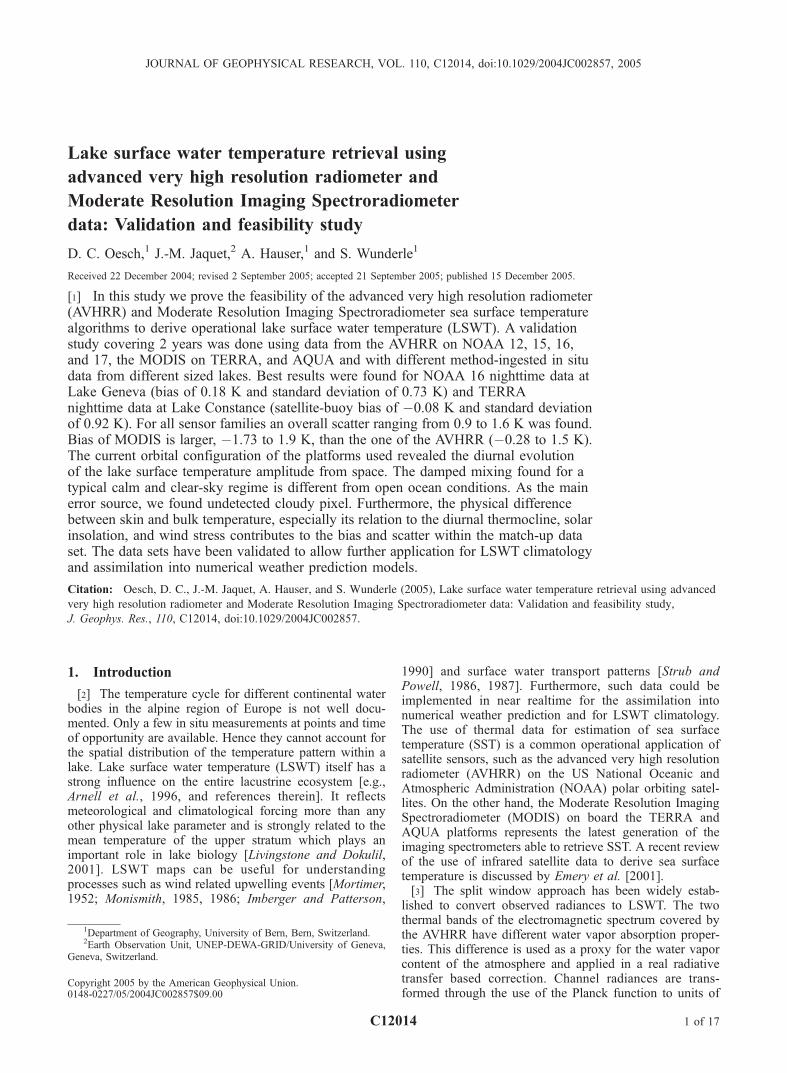
[10] Regional validation needs a higher temporal resolu-tion than global applications, where match-ups are madewithin 4h considering the diurnal warming effect [Boehm etal., 1991; Hawkins et al., 1993]. Three lakes located at thenorthwestern rim of the European Alps offer in situ datawith a temporal resolution of at least 60 min (Figures 1, 2,and 3 and Table 1) and meet with the recommendation by

Minnett [1991] that validation measurements should bemade within ±2h of the satellite overpass. The two largestwaterbodies, Lake Geneva (Figure 1) and Lake Constance(Figure 2), have both a monomictic mixing regime and aremesotrophic. Water budget and lake levels reflect theseasonality of the alpine climate which retains snow duringthe winter. The lake levels are maximum in early summerand minimum during winter.[11] Lake Geneva is the largest lake in the Alpine region.

The Rhone River discharges at the eastern tip and flowssouthward from the west end of the lake to the Mediterra-nean Sea. The lake is deep and has a comparatively largewater volume for its surface area (Table 1). The drainagebasin is fairly large, including about half of the Valais andBernese Alps. The in situ water temperature is recorded bythe Swiss Federal Institute of Technology (Lausanne) at thenorth shore of the lake near Buchillon on a pylon located100 m offshore (46.4584�N/6.3996�E) over a water depth of3–4 m near the vicinity of Buchillion (point P1 in Figure 1).The pylon is equipped with meteorological sensors (e.g.,wind speed and shortwave net radiation) and a watertemperature probe measuring at approximately 1 m depth.The data is sampled to hourly averages. A continuous dataset from 31 January 2002 to 12 December 2003 is available.This station is representative of the shallow littoral waterbody, which has a temperature regime different from theopen water [Fer et al., 2001, 2002].[12] Lake Constance is the second largest European

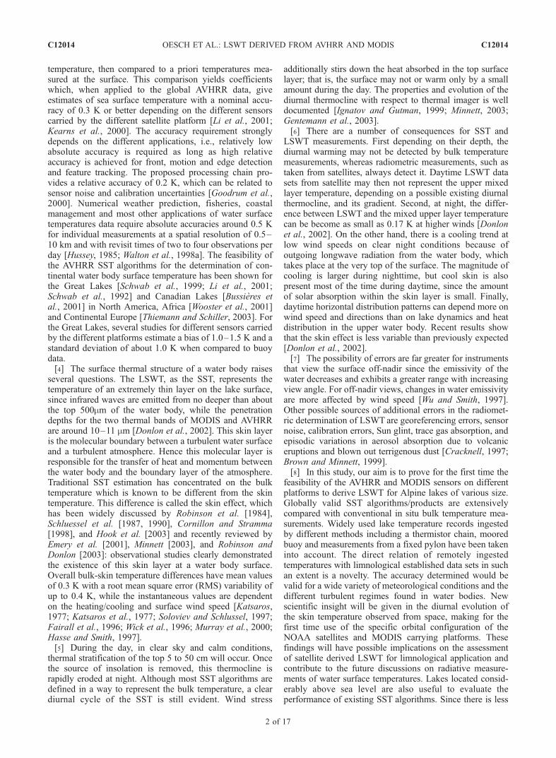
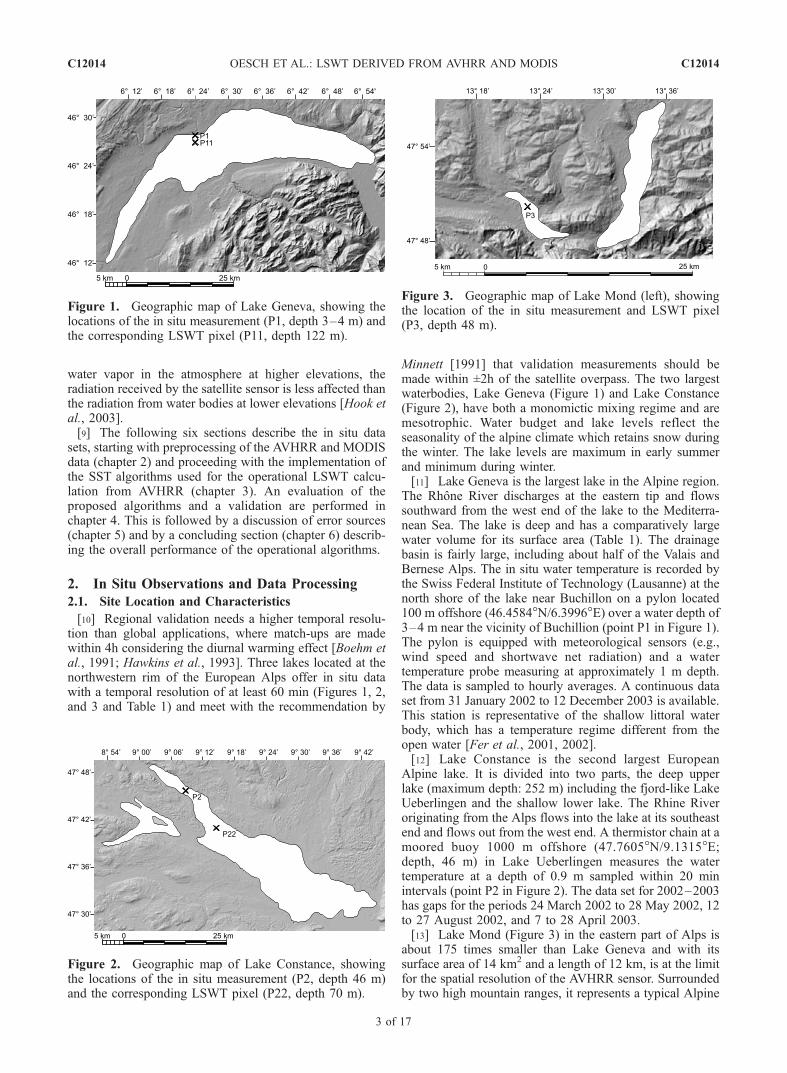
Alpine lake. It is divided into two parts, the deep upperlake (maximum depth: 252 m) including the fjord-like LakeUeberlingen and the shallow lower lake. The Rhine Riveroriginating from the Alps flows into the lake at its southeastend and flows out from the west end. A thermistor chain at amoored buoy 1000 m offshore (47.7605�N/9.1315�E;depth, 46 m) in Lake Ueberlingen measures the watertemperature at a depth of 0.9 m sampled within 20 minintervals (point P2 in Figure 2). The data set for 2002–2003has gaps for the periods 24 March 2002 to 28 May 2002, 12to 27 August 2002, and 7 to 28 April 2003.[13] Lake Mond (Figure 3) in the eastern part of Alps is

about 175 times smaller than Lake Geneva and with itssurface area of 14 km2 and a length of 12 km, is at the limitfor the spatial resolution of the AVHRR sensor. Surroundedby two high mountain ranges, it represents a typical Alpine

Figure 1. Geographic map of Lake Geneva, showing thelocations of the in situ measurement (P1, depth 3–4 m) andthe corresponding LSWT pixel (P11, depth 122 m).

Figure 2. Geographic map of Lake Constance, showingthe locations of the in situ measurement (P2, depth 46 m)and the corresponding LSWT pixel (P22, depth 70 m).

Figure 3. Geographic map of Lake Mond (left), showingthe location of the in situ measurement and LSWT pixel(P3, depth 48 m).


3 of 17

C12014

Lake. It is oligo-mesotrophic and discharges into a smallriver. The catchment area mostly consists of an Alpineenvironment of forest and grassland. A moored buoyapproximately 1000 m offshore at point P3 in Figure 3(47.8374�N/13.3686�E; depth, 48 m) measures the watertemperature at 1 m depth using a Yellow Springs Multi-sonde 6920. The data sampling is done in 60 min intervals.The data set 2002–2003 is continuously available exceptfor a data gap from 25 January 2002 to 16 May 2002.[14] As can be seen in Figures 1 and 2, P1 and P2 are

located relatively close to the shore. Because of the spatialresolution of the sensors used in this study, the corre-sponding satellite image pixel of P1 and P2 can partlyinclude land surface information. This can significantly alterthe radiometric signal of the water surface. During night-time, because of the greater heat storage capacity of a waterbody, land contamination can imply a cooling effect, whileduring daytime the opposite can be the case. For both sensorproducts, different land masks where used to flag possibleland contaminated pixels. The land mask applied on theAVHRR LSWT is based on the global self-consistenthierarchical high-resolution shoreline database (GSHHRS)[Wessel and Smith, 1996]. In addition to the GSHHRS, ashore buffer zone with size of one pixel has been flagged.The land discrimination scheme in the MODIS SST productbeing more stringent, no additional buffer zone was applied.Therefore, for the validation process, we chose P11(46.4439�N/6.3996�E; depth , 125 m) and P22(47.6841�N/9.2384�E; depth, 70 m) as the closestcorresponding pure water pixels for P1 and P2. Since theproperties of the water bodies at P11 and P22 are differentfrom P1 and P2, one can assume that because of internalseiches, there might exist significant temperature differ-ences between the in situ and LSWT pixel locations.However, the validation of AVHRR at P1 and P2, ignoringthe buffer zone, showed similar results as at thecorresponding P11 and P22 location. The number of coin-cident data points was smaller and the bias and scatterslightly higher, since the nearshore data (P1, P2) are moreaffected by land contamination. Therefore we choose in thisstudy to use LSWT pixel location P11 as substitute for P1,respectively P22 for P2.

2.2. AVHRR Data

[15] The data presented in this paper uses observationsfrom the five channel AVHRR/2 (NOAA 12) and the sixchannel AVHRR/3 (NOAA 15, 16, and 17) instruments onboard the NOAA polar satellites. The instruments measurereflected and emitted radiance in the following bands:0.58–0.68 mm (channel 1), 0.725–1.10 mm (channel 2),1.57–1.64 mm (channel 3a on AVHRR/3), 3.55–3.93 mm(channel 3b on AVHRR/3 and channel 3 on AVHRR/2),

10.3–11.3 mm (channel 4), and 11.5–12.5 mm (channel 5).The nominal instrument spatial resolution is 1.1 km.[16] The orbital configuration of the NOAA polar satel-

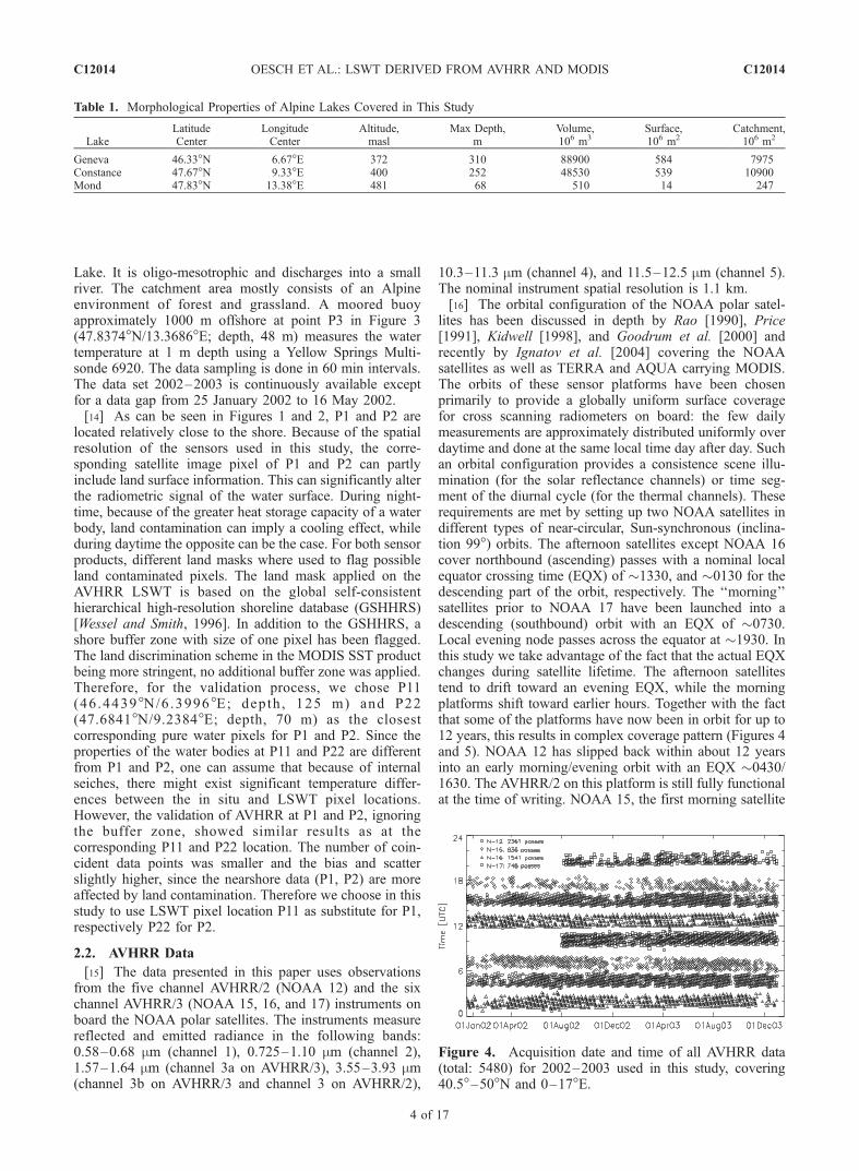
lites has been discussed in depth by Rao [1990], Price[1991], Kidwell [1998], and Goodrum et al. [2000] andrecently by Ignatov et al. [2004] covering the NOAAsatellites as well as TERRA and AQUA carrying MODIS.The orbits of these sensor platforms have been chosenprimarily to provide a globally uniform surface coveragefor cross scanning radiometers on board: the few dailymeasurements are approximately distributed uniformly overdaytime and done at the same local time day after day. Suchan orbital configuration provides a consistence scene illu-mination (for the solar reflectance channels) or time seg-ment of the diurnal cycle (for the thermal channels). Theserequirements are met by setting up two NOAA satellites indifferent types of near-circular, Sun-synchronous (inclina-tion 99�) orbits. The afternoon satellites except NOAA 16cover northbound (ascending) passes with a nominal localequator crossing time (EQX) of �1330, and �0130 for thedescending part of the orbit, respectively. The ‘‘morning’’satellites prior to NOAA 17 have been launched into adescending (southbound) orbit with an EQX of �0730.Local evening node passes across the equator at �1930. Inthis study we take advantage of the fact that the actual EQXchanges during satellite lifetime. The afternoon satellitestend to drift toward an evening EQX, while the morningplatforms shift toward earlier hours. Together with the factthat some of the platforms have now been in orbit for up to12 years, this results in complex coverage pattern (Figures 4and 5). NOAA 12 has slipped back within about 12 yearsinto an early morning/evening orbit with an EQX �0430/1630. The AVHRR/2 on this platform is still fully functionalat the time of writing. NOAA 15, the first morning satellite

Table 1. Morphological Properties of Alpine Lakes Covered in This Study

LakeLatitudeCenter

LongitudeCenter

Altitude,masl

Max Depth,m

Volume,106 m3

Surface,106 m2

Catchment,106 m2

Geneva 46.33�N 6.67�E 372 310 88900 584 7975Constance 47.67�N 9.33�E 400 252 48530 539 10900Mond 47.83�N 13.38�E 481 68 510 14 247

Figure 4. Acquisition date and time of all AVHRR data(total: 5480) for 2002–2003 used in this study, covering40.5�–50�N and 0–17�E.


4 of 17

C12014

with the AVHRR/3 on board, lost since his launch in spring1998 about 40 min (current EQX �0650/1650). The deg-radation of the NOAA 15 AVHRR/3 is substantial but thethermal data is still useful. A modified afternoon orbit withan EQX �1400 (northbound node) was chosen for NOAA16. A special technical effort was made to stabilize theorbits of satellites carrying the AVHRR/3, so the EQX ofNOAA 16 did not change significantly within the 3 yearssince launch. Nevertheless, the AVHRR/3 scan motorstarted to become erroneous on 18 September 2003. Thelast gap for a uniform daily coverage was closed by settingNOAA 17 into a new midmorning orbit with an EQX of�1000.[17] The orbits of NOAA 16 and 17 are quite similar to

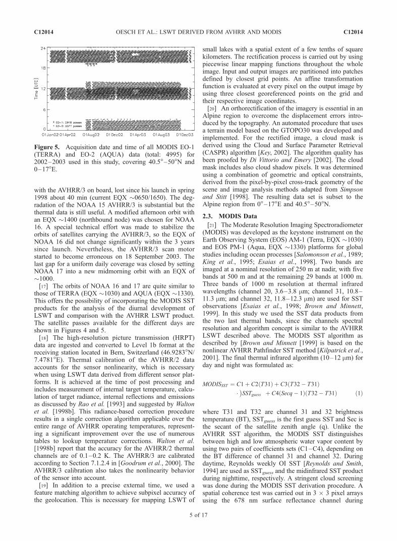
those of TERRA (EQX �1030) and AQUA (EQX �1330).This offers the possibility of incorporating the MODIS SSTproducts for the analysis of the diurnal development ofLSWT and comparison with the AVHRR LSWT product.The satellite passes available for the different days areshown in Figures 4 and 5.[18] The high-resolution picture transmission (HRPT)

data are ingested and converted to Level 1b format at thereceiving station located in Bern, Switzerland (46.9283�N/7.4781�E). Thermal calibration of the AVHRR/2 dataaccounts for the sensor nonlinearity, which is necessarywhen using LSWT data derived from different sensor plat-forms. It is achieved at the time of post processing andincludes measurement of internal target temperature, calcu-lation of target radiance, internal reflections and emissionsas discussed by Rao et al. [1993] and suggested by Waltonet al. [1998b]. This radiance-based correction procedureresults in a single correction algorithm applicable over theentire range of AVHRR operating temperatures, represent-ing a significant improvement over the use of numeroustables to lookup temperature corrections. Walton et al.[1998b] report that the accuracy for the AVHRR/2 thermalchannels are of 0.1–0.2 K. The AVHRR/3 are calibratedaccording to Section 7.1.2.4 in [Goodrum et al., 2000]. TheAVHRR/3 calibration also takes the nonlinearity behaviorof the sensor into account.[19] In addition to a precise external time, we used a

feature matching algorithm to achieve subpixel accuracy ofthe geolocation. This is necessary for mapping LSWT of

small lakes with a spatial extent of a few tenths of squarekilometers. The rectification process is carried out by usingpiecewise linear mapping functions throughout the wholeimage. Input and output images are partitioned into patchesdefined by closest grid points. An affine transformationfunction is evaluated at every pixel on the output image byusing three closest georeferenced points on the grid andtheir respective image coordinates.[20] An orthorectification of the imagery is essential in an

Alpine region to overcome the displacement errors intro-duced by the topography. An automated procedure that usesa terrain model based on the GTOPO30 was developed andimplemented. For the rectified image, a cloud mask isderived using the Cloud and Surface Parameter Retrieval(CASPR) algorithm [Key, 2002]. The algorithm quality hasbeen proofed by Di Vittorio and Emery [2002]. The cloudmask includes also cloud shadow pixels. It was determinedusing a combination of geometric and optical constraints,derived from the pixel-by-pixel cross-track geometry of thescene and image analysis methods adapted from Simpsonand Stitt [1998]. The resulting data set is subset to theAlpine region from 0�–17�E and 40.5�–50�N.

2.3. MODIS Data

[21] The Moderate Resolution Imaging Spectroradiometer(MODIS) was developed as the keystone instrument on theEarth Observing System (EOS) AM-1 (Terra, EQX �1030)and EOS PM-1 (Aqua, EQX �1330) platforms for globalstudies including ocean processes [Salomonson et al., 1989;King et al., 1995; Esaias et al., 1998]. Two bands areimaged at a nominal resolution of 250 m at nadir, with fivebands at 500 m and at the remaining 29 bands at 1000 m.Three bands of 1000 m resolution at thermal infraredwavelengths (channel 20, 3.6–3.8 mm; channel 31, 10.8–11.3 mm; and channel 32, 11.8–12.3 mm) are used for SSTobservations [Esaias et al., 1998; Brown and Minnett,1999]. In this study we used the SST data products fromthe two last thermal bands, since the channels spectralresolution and algorithm concept is similar to the AVHRRLSWT described above. The MODIS SST algorithm asdescribed by [Brown and Minnett [1999] is based on thenonlinear AVHRR Pathfinder SST method [Kilpatrick et al.,2001]. The final thermal infrared algorithm (10–12 mm) forday and night was formulated as:

MODISSST ¼ C1þ C2 T31ð Þ þ C3 T32� T31ð Þ� SSTguess� �

þ C4 Secq� 1ð Þ T32� T31ð Þ ð1Þ

where T31 and T32 are channel 31 and 32 brightnesstemperature (BT), SSTguess is the first guess SST and Sec isthe secant of the satellite zenith angle (q). Unlike theAVHRR SST algorithm, the MODIS SST distinguishesbetween high and low atmospheric water vapor content byusing two pairs of coefficients sets (C1–C4), depending onthe BT difference of channel 31 and channel 32. Duringdaytime, Reynolds weekly OI SST [Reynolds and Smith,1994] are used as SSTguess and the midinfrared SST productduring nighttime, respectively. A stringent cloud screeningwas done during the MODIS SST derivation procedure. Aspatial coherence test was carried out in 3 � 3 pixel arraysusing the 678 nm surface reflectance channel during

Figure 5. Acquisition date and time of all MODIS EO-1(TERRA) and EO-2 (AQUA) data (total: 4995) for2002–2003 used in this study, covering 40.5�–50�N and0–17�E.


5 of 17

C12014

daytime and thermal channels at nighttime. Finally, theretrieved SST were tested against Reynolds weekly OI SSTand rejected if the discrepancy was greater than 6 K.[22] Comparisons of MODIS TERRA SSTs and collo-

cated skin SST measurements from the Marine Atmo-spheric Emitted Radiance Interferometer (MAERI) led toan additional empirical correction [Minnett et al., 2001].However, Minnett et al. [2002] showed that the MODISSSTs are comparable in accuracy to the AVHRR Path-finder SST fields.[23] In this study we used MODIS TERRA and AQUA

Sea Surface Temperature Products 5-Min L2 Swath 1 km(MOD28L2 and MYD28L2) data of the years 2002 and2003. The data were provided by the NASA/Goddard EarthSciences Distributed Active Archive Center (GES DAAC)at http://daac.gsfc.nasa.gov/. The MODIS SST productswere available in their third release (Collection 4). Thosedata sets are considered as validated products in a maturestage. All data sets covering the area of 0�–17�E and40.5�–50�N were subset and stitched together to alatitude/longitude grid with the same dimension as theAVHRR data sets. The data available for the different daysare shown in Figure 5.

3. Implementation of the AVHRR LSWT Method

[24] The different water vapor absorption properties ofthe two thermal bands of the AVHRR are used to correct forthe effects of the atmosphere on the observations of theinfrared signal emitted by the surface. A slight but notnegligible distortion of the infrared channels in this spec-trum is due to absorption of water vapor. The split windowtechnique utilizes the difference between channel 4 andchannel 5 to correct this effect: the temperature differencebetween these two channels is proportional to the amount ofwater vapor in the atmosphere because infrared radiationundergoes a stronger absorption because of atmosphericmoisture within channel 5 than within channel 4. Anotheradvantage of the split window approach is the fact that ittakes the varying atmospheric path length variations withthe satellite viewing angle into account. The SST methodensures that the mean SST temperatures can be comparedwith bulk temperatures [Barton and Prata, 1995; Wick andBates, 2002]. Two algorithms based on the split windowtheory are commonly used for water surface temperaturederivation. The multichannel SST (MCSST) algorithmwas developed and used operationally at NOAA/NESDIS(National Environmental Satellite Data and InformationService) in the early eighties on the basis of the work byMcClain et al. [1985]. This algorithm assumes that there is alinear relationship between the difference of the satellitebrightness temperatures and bulk temperature and the dif-ference of satellite measurements in the split windowchannels. Coefficients B2 and B3 in equation (3) werefound to be slightly nonlinear, having a dependency onboth atmospheric water vapor and the brightness tempera-ture itself, particularity in dry polar and moist tropicalregions. Considering rather a nonlinear term, an operationalnonlinear SST (NLSST) algorithm for the NOAA polarorbiting satellites was implemented in 1991, resulting in lessscatter when comparing satellite SST against drifting buoydata [Walton, 1988; Walton et al., 1998a]. For both algo-

rithms, coefficients are routinely obtained for the operationalsensor platforms by performing a regression using a match-up database of satellite retrievals and buoy data. Unfortu-nately, after a sensor platform is no longer operational noupdates are available. The NLSST uses the MCSST as a firstestimate of sea surface temperature for the nonlinear term ofthe equation.[25] For night and day passes, different coefficients for

the equations are applied, which are provided by NOAA/NESDIS as described by Walton et al. [1998a]. The coef-ficients are independent of season, geographic location oratmospheric moisture content. Adjustments are necessary ifspacecraft instrument calibration change or backgroundaerosol content in the stratosphere is affected by volcaniceruptions.[26] When applying this method to continental water-

bodies, such as the North American Great Lakes, theaccuracy of LSWT estimation shows a bias of 0.5 K orbetter depending on the different sensors of the differentsatellite platform [Schwab et al., 1999; Li et al., 2001].The root mean square error (RMS) ranges from 1.1 to1.7 K.[27] The form of the LSWT retrieval algorithms used in

this paper has been developed by Walton et al. [1998a] andapplied by Li et al. [2001] as:

NLSST ¼ A1 T11ð Þ þ A2 T11� T12ð Þ MCSSTð Þþ A3 T11� T12ð Þ Secq� 1ð Þ � A4 ð2Þ

MCSST ¼ B1 T11ð Þ þ B2 T11� T12ð Þþ B3 T11� T12ð Þ Secq� 1ð Þ � B4 ð3Þ

T11 and T12 are channel 4 and 5 temperatures in Kelvin;Secq is the secant of the satellite zenith angle q; NLSST andMCSST are the nonlinear and linear multichannel SST,respectively, in degrees Celsius; A1–A4 and B1–B4 are thecoefficients according to NESDIS. The valid range of theNLSST approach ranges from �5� to 30�C.[28] The equations used in this paper differ from the

global SST equations in the following aspects: on the onehand we used the MCSST value in the nonlinear term ratherthan an a priori SST estimate obtained from an analysis ofpast satellite SST data. This means that there is somewhatmore noise in the LSWT observations. The value of the apriori SST or the MCSST is constrained to the range 0�C to30�C. On the other hand, the NLSST split window equationis used here rather than the triple window equation (employ-ing all three infrared channels) which is used in the globaloperation.[29] To maintain high accuracy of LSWT algorithm, pixel

viewed with a satellite zenith angle greater than 53� areomitted, since a larger atmospheric path length leads togreater attenuation of surface emitted radiance.[30] Day (Sun zenith less than 75�) and night (Sun zenith

greater than 75�) algorithms have been implemented in thisstudy.[31] As described above, possible land contaminated

LSWT pixels and a one-pixel wide buffer zone wereflagged. A threshold scheme is used to mask out cloudcontaminated pixel, which are not detected by CASPR.


6 of 17

C12014

During daytime, a gross infrared test and visible cloudthreshold test is performed: pixels with channel 4 temper-atures lower than �5�C or a corrected albedo (albedo valuedivided by the cosine of the solar zenith angle) greater thanten percent are considered as cloud contaminated. The grossinfrared (IR) test is also used for night satellite imagerytogether with a test for low stratus clouds: The differenceobtained when subtracting channel 3 temperature fromchannel 5 temperature must be less than or equal to�0.6 K. Finally, as Schwab et al. [1999] suggested, pixelswith a standard deviation greater than 3 K computed of theneighboring pixels and pixels completely surrounded bynonvalid data are rejected.

4. Validation

4.1. Results AVHRR

[32] The performance of the MCSST and NLSST algo-rithms were tested for NOAA 12, 15, 16, and 17 in the timeperiod of 2002 and 2003 for all three lakes. From the 5480ingested data files (Figure 4), a total of 1838 match-ups forMCSST and 1856 for NLSST were available (Lake Geneva,547/548; Lake Constance, 774/778; and Lake Mond,517/530). At all in situ locations and for each satellite passthe corresponding pixel LSWT was compared to the in situtemperature closest to the satellite overpass, not exceeding atime difference of 30 min. The scatterplots of LSWT versusin situ measurement for the different algorithms are given inFigure 6 for Lake Geneva, Figure 7 for Lake Constance, andFigure 8 for Lake Mond. The statistical results (satellite-buoy bias, standard deviation (s) and the squared correla-tion coefficient (r2), the number of match-ups and the RMSerror of the regression LSWT on in situ temperature areshown Figures 6–8.[33] For the various data sets corresponding to different

locations, sensors and algorithms, LSWT data outside therange of ±2 standard deviations was flagged, and removedfrom the match-up database. Within the 2 sigma interval,over 95 percent of the data can be found, assuming anormal distribution. Significant differences between the insitu measurement and the LSWT can occur for severalreasons. (a) Sub pixel cloud contamination has often a coldbias effect. (b) LSWT within a pixel can vary severaldegrees, particularly nearshore and in smaller lakes. Thiscan be related to thermal fronts and other circulationprocesses related to lake physics. (c) The AVHRR LSWTdata with a warm bias has different sources. As describedby Khattak et al. [1991], Sun glint can introduce a bias upto 2 K. For several warm biased outliers of NOAA 12 and15 day passes, Sun glint could be identified over the waterbodies.[34] After the exclusion of the match-ups beyond ±2 stan-

dard deviations, the remaining data set totals (MCSST/NLSST) were 515/518 for Lake Geneva, 733/735 for LakeConstance and 459/498 for Lake Mond. Using this methodto remove outliers, we excluded only about 6% of theoriginal match-up database.[35] As a more general result we can state for Figures 6,

7, and 8 that we have a larger amount of match-ups coveringhigher summer temperatures, which tend to have a warmerLSWT bias. Likewise, another accumulation of coincidentdata can be found for lower winter temperatures, where we

can observe a cool bias, compared to the 1:1 line. For thenighttime match-up, the warm offset of the LSWT is smalleras are also the scatter and bias when compared to daytime.Considering the outliers, more warm outliers were foundduring hours of daylight and more cold outliers duringnighttime. In this study, the smallest bias and scatter werefound for the NOAA 16 for Lake Geneva MCSST nighttimewith 0.18 and 0.73 K, respectively. The performance of theLSWT can be examined with respect to the followingcriteria: day/night algorithm, in situ measurement/lake andsatellite number.4.1.1. Performance of the Different Algorithmsand Sensors[36] The linear SST equation (MCSST) yields a slightly

better overall accuracy than the nonlinear algorithm(NLSST), as can be seen in Figures 6, 7, and 8. Especiallyduring daytime, the MCSST has a lower bias than NLSSTfor all sensors in all three lakes (overall MCSST/NLSSTday bias: 1.21 K/1.92 K). This fact has also been observedfor the Great Lakes by Li et al. [2001]. For nighttime data,MCSST showed better results. The only exception is forLake Mond, where the bias was quite high with an overallbetter performance of the NLSST. For both algorithms, thestandard deviation was with 1.35 K (MCSST) and 1.34 K(NLSST) about the same, whereas the bias of the MCSSTwas with 0.55 K lower than for the nonlinear approach(1.16 K).[37] The best overall achievement of the different satel-

lites sensors was found for NOAA 16 with an average biasof 0.24 K and standard deviation of 1.48 K for the MCSSTalgorithm. As can be seen in Figures 6–8, NOAA 12showed generally a larger offset (average up to 2 K). TheMCSST/NLSST coefficients of NOAA 12 have not beenupdated since 1994 and might therefore be out of date.Furthermore, the EQX of NOAA 12 shifted over the yearsof operation to twilight phases of the day, where the remotesensing of LSWT is done at low Sun angles conditions.Since only day or nighttime coefficients were available, thecorrection introduced to the brightness temperature canyield the higher bias observed in Figures 6–8. Additionally,the cloud masking during dawn is more susceptible to omitcloud pixel than for large Sun zenith angles or at nighttimerespectively. This results in a larger match-up database forNOAA 12 day/night data, with larger standard deviationand bias.[38] The warm bias of the LSWT for the higher daytime

temperatures can be observed for the NLSST as well as forthe MCSST algorithm. This is due to the formation of ashallow diurnal layer, which results in the skin temperatureappearing to be warm. Relative to the temperature justbelow the surface, the LSWT is still cool, but comparedto the deeper bulk temperature it appears to be warmer.During nighttime the warm bias diminishes especially forthe MCSST data for Lake Constance, where it becomesmarginal. At Lake Mond, the bias becomes negative atnighttime for all sensors using the linear term, and only forthe nonlinear data set for N12 and erved for all AVHRRdata except N15 during nighttime. At all locations, the nightalgorithm has a smaller bias (MCSST, �0.4 K and NLSST,0.4 K) and standard deviation (1.1 K) than thecorresponding daytime method (bias: 1.2 K (MCSST)/1.9 K (NLSST), standard deviation: 1.5 K).


7 of 17

C12014

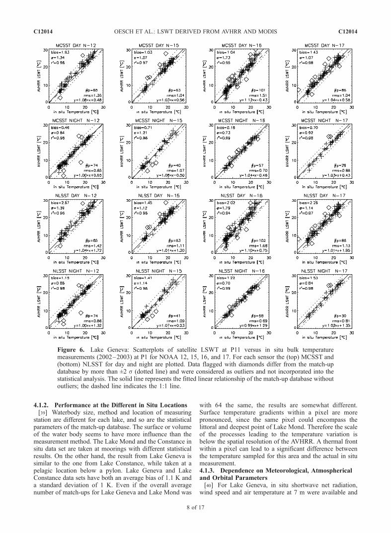
4.1.2. Performance at the Different in Situ Locations[39] Waterbody size, method and location of measuring

station are different for each lake, and so are the statisticalparameters of the match-up database. The surface or volumeof the water body seems to have more influence than themeasurement method. The Lake Mond and the Constance insitu data set are taken at moorings with different statisticalresults. On the other hand, the result from Lake Geneva issimilar to the one from Lake Constance, while taken at apelagic location below a pylon. Lake Geneva and LakeConstance data sets have both an average bias of 1.1 K anda standard deviation of 1 K. Even if the overall averagenumber of match-ups for Lake Geneva and Lake Mond was

with 64 the same, the results are somewhat different.Surface temperature gradients within a pixel are morepronounced, since the same pixel could encompass thelittoral and deepest point of Lake Mond. Therefore the scaleof the processes leading to the temperature variation isbelow the spatial resolution of the AVHRR. A thermal frontwithin a pixel can lead to a significant difference betweenthe temperature sampled for this area and the actual in situmeasurement.4.1.3. Dependence on Meteorological, Atmosphericaland Orbital Parameters[40] For Lake Geneva, in situ shortwave net radiation,

wind speed and air temperature at 7 m were available and

Figure 6. Lake Geneva: Scatterplots of satellite LSWT at P11 versus in situ bulk temperaturemeasurements (2002–2003) at P1 for NOAA 12, 15, 16, and 17. For each sensor the (top) MCSST and(bottom) NLSST for day and night are plotted. Data flagged with diamonds differ from the match-updatabase by more than ±2 s (dotted line) and were considered as outliers and not incorporated into thestatistical analysis. The solid line represents the fitted linear relationship of the match-up database withoutoutliers; the dashed line indicates the 1:1 line.


8 of 17

C12014

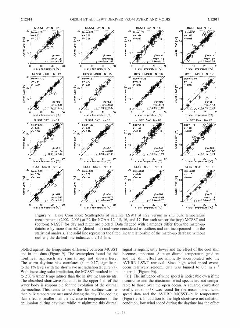
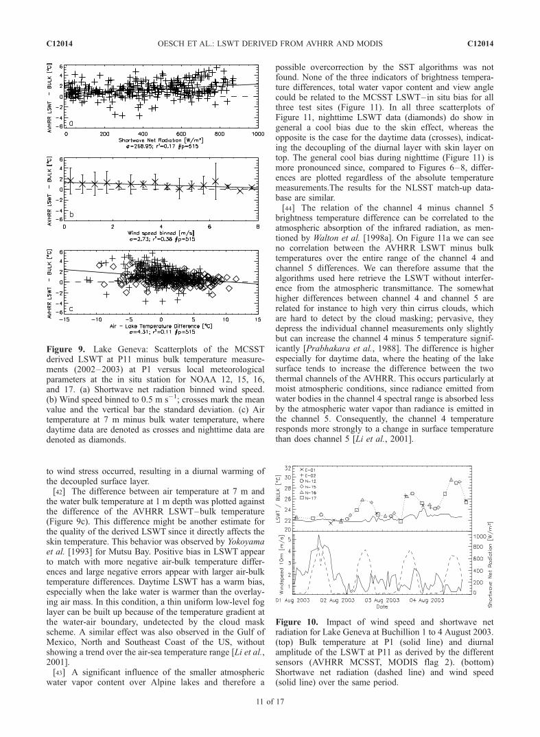
plotted against the temperature difference between MCSSTand in situ data (Figure 9). The scatterplots found for thenonlinear approach are similar and not shown here.The warm daytime bias correlates (r2 = 0.17, significantto the 1% level) with the shortwave net radiation (Figure 9a).With increasing solar irradiation, the MCSST resulted in upto 2 K warmer temperatures than the in situ measurements.The absorbed shortwave radiation in the upper 1 m of thewater body is responsible for the evolution of the diurnalthermocline. This tends to make the skin surface warmerthan bulk temperature measured during the day. The coolingskin effect is smaller than the increase in temperature in theepilimnion during daytime, while at nighttime this diurnal

signal is significantly lower and the effect of the cool skinbecomes important. A mean diurnal temperature gradientand the skin effect are implicitly incorporated into theAVHRR LSWT retrieval. Since high wind speed eventsoccur relatively seldom, data was binned to 0.5 m s�1

intervals (Figure 9b).[41] The influence of wind speed is noticeable even if the

occurrence and the maximum wind speeds are not compa-rable to those over the open ocean. A squared correlationcoefficient of 0.38 was found for the mean binned windspeed data and the AVHRR MCSST–bulk temperature(Figure 9b). In addition to the high shortwave net radiationcondition, low wind speed during the daytime has the effect

Figure 7. Lake Constance: Scatterplots of satellite LSWT at P22 versus in situ bulk temperaturemeasurements (2002–2003) at P2 for NOAA 12, 15, 16, and 17. For each sensor the (top) MCSST and(bottom) NLSST for day and night are plotted. Data flagged with diamonds differ from the match-updatabase by more than ±2 s (dotted line) and were considered as outliers and not incorporated into thestatistical analysis. The solid line represents the fitted linear relationship of the match-up database withoutoutliers; the dashed line indicates the 1:1 line.


9 of 17

C12014

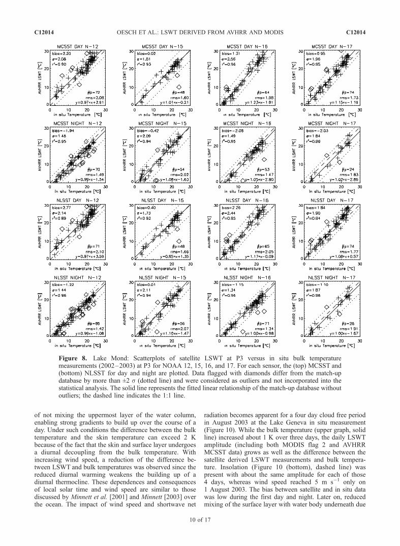
of not mixing the uppermost layer of the water column,enabling strong gradients to build up over the course of aday. Under such conditions the difference between the bulktemperature and the skin temperature can exceed 2 Kbecause of the fact that the skin and surface layer undergoesa diurnal decoupling from the bulk temperature. Withincreasing wind speed, a reduction of the difference be-tween LSWT and bulk temperatures was observed since thereduced diurnal warming weakens the building up of adiurnal thermocline. These dependences and consequencesof local solar time and wind speed are similar to thosediscussed by Minnett et al. [2001] and Minnett [2003] overthe ocean. The impact of wind speed and shortwave net

radiation becomes apparent for a four day cloud free periodin August 2003 at the Lake Geneva in situ measurement(Figure 10). While the bulk temperature (upper graph, solidline) increased about 1 K over three days, the daily LSWTamplitude (including both MODIS flag 2 and AVHRRMCSST data) grows as well as the difference between thesatellite derived LSWT measurements and bulk tempera-ture. Insolation (Figure 10 (bottom), dashed line) waspresent with about the same amplitude for each of those4 days, whereas wind speed reached 5 m s�1 only on1 August 2003. The bias between satellite and in situ datawas low during the first day and night. Later on, reducedmixing of the surface layer with water body underneath due

Figure 8. Lake Mond: Scatterplots of satellite LSWT at P3 versus in situ bulk temperaturemeasurements (2002–2003) at P3 for NOAA 12, 15, 16, and 17. For each sensor, the (top) MCSST and(bottom) NLSST for day and night are plotted. Data flagged with diamonds differ from the match-updatabase by more than ±2 s (dotted line) and were considered as outliers and not incorporated into thestatistical analysis. The solid line represents the fitted linear relationship of the match-up database withoutoutliers; the dashed line indicates the 1:1 line.


10 of 17

C12014

to wind stress occurred, resulting in a diurnal warming ofthe decoupled surface layer.[42] The difference between air temperature at 7 m and

the water bulk temperature at 1 m depth was plotted againstthe difference of the AVHRR LSWT–bulk temperature(Figure 9c). This difference might be another estimate forthe quality of the derived LSWT since it directly affects theskin temperature. This behavior was observed by Yokoyamaet al. [1993] for Mutsu Bay. Positive bias in LSWT appearto match with more negative air-bulk temperature differ-ences and large negative errors appear with larger air-bulktemperature differences. Daytime LSWT has a warm bias,especially when the lake water is warmer than the overlay-ing air mass. In this condition, a thin uniform low-level foglayer can be built up because of the temperature gradient atthe water-air boundary, undetected by the cloud maskscheme. A similar effect was also observed in the Gulf ofMexico, North and Southeast Coast of the US, withoutshowing a trend over the air-sea temperature range [Li et al.,2001].[43] A significant influence of the smaller atmospheric

water vapor content over Alpine lakes and therefore a

possible overcorrection by the SST algorithms was notfound. None of the three indicators of brightness tempera-ture differences, total water vapor content and view anglecould be related to the MCSST LSWT–in situ bias for allthree test sites (Figure 11). In all three scatterplots ofFigure 11, nighttime LSWT data (diamonds) do show ingeneral a cool bias due to the skin effect, whereas theopposite is the case for the daytime data (crosses), indicat-ing the decoupling of the diurnal layer with skin layer ontop. The general cool bias during nighttime (Figure 11) ismore pronounced since, compared to Figures 6–8, differ-ences are plotted regardless of the absolute temperaturemeasurements.The results for the NLSST match-up data-base are similar.[44] The relation of the channel 4 minus channel 5

brightness temperature difference can be correlated to theatmospheric absorption of the infrared radiation, as men-tioned by Walton et al. [1998a]. On Figure 11a we can seeno correlation between the AVHRR LSWT minus bulktemperatures over the entire range of the channel 4 andchannel 5 differences. We can therefore assume that thealgorithms used here retrieve the LSWT without interfer-ence from the atmospheric transmittance. The somewhathigher differences between channel 4 and channel 5 arerelated for instance to high very thin cirrus clouds, whichare hard to detect by the cloud masking; pervasive, theydepress the individual channel measurements only slightlybut can increase the channel 4 minus 5 temperature signif-icantly [Prabhakara et al., 1988]. The difference is higherespecially for daytime data, where the heating of the lakesurface tends to increase the difference between the twothermal channels of the AVHRR. This occurs particularly atmoist atmospheric conditions, since radiance emitted fromwater bodies in the channel 4 spectral range is absorbed lessby the atmospheric water vapor than radiance is emitted inthe channel 5. Consequently, the channel 4 temperatureresponds more strongly to a change in surface temperaturethan does channel 5 [Li et al., 2001].

Figure 9. Lake Geneva: Scatterplots of the MCSSTderived LSWT at P11 minus bulk temperature measure-ments (2002–2003) at P1 versus local meteorologicalparameters at the in situ station for NOAA 12, 15, 16,and 17. (a) Shortwave net radiation binned wind speed.(b) Wind speed binned to 0.5 m s�1; crosses mark the meanvalue and the vertical bar the standard deviation. (c) Airtemperature at 7 m minus bulk water temperature, wheredaytime data are denoted as crosses and nighttime data aredenoted as diamonds.

Figure 10. Impact of wind speed and shortwave netradiation for Lake Geneva at Buchillion 1 to 4 August 2003.(top) Bulk temperature at P1 (solid line) and diurnalamplitude of the LSWT at P11 as derived by the differentsensors (AVHRR MCSST, MODIS flag 2). (bottom)Shortwave net radiation (dashed line) and wind speed(solid line) over the same period.


11 of 17

C12014

[45] Furthermore, it could be proved that the performanceof the split window method used is independent of the watervapor content of the atmosphere derived from thecorresponding grid cell of the limited area atmosphericprediction model Local Model of the Consortium forSmall-Scale Modeling [Doms and Schattler, 2002; Schraffand Hess, 2003] with the horizontal resolution of 7 km �7 km (Figure 11b). Atmospheric path length of the infraredsignal could not be related to the bias (Figure 11c). TheNOAA/NESDIS SST coefficients are independent of thesatellite zenith angle over the whole range from 0–53�.

4.2. MODIS Results

[46] The performance of the MODIS SST products withquality flag 1 (questionable) and 2 (probably cloud) weretested for the Lake Geneva and the Lake Constance in situmeasurement. As for AVHRR, match-ups were derived forthe MODIS SST data where an in situ measurement within30 min was available. The total MODIS SST match-updatabase was of the size of 1068 (Lake Geneva: 576 LakeConstance: 492). The number of match-ups flagged withquality 0 (good) was less than 30 for all algorithms for Lake

Constance and most for Lake Geneva, so flag 0 data wasdisregarded in this study.[47] For Lake Mond, only flag 2 (probably cloudy)

nighttime data was available and therefore not taken intoaccount in this study. Scatterplots of the match-up databasefor day and night passes for TERRA (EO-1) and AQUA(EO-2) are shown in Figure 12 for Lake Geneva andFigure 13 for Lake Constance.[48] The validation results are dependent on the EO

platform algorithm, the quality flag and the lake. For

Figure 11. Scatterplots of the MCSST derived LSWT atminus bulk temperature measurements (2002–2003) versusparameters representing the atmospheric water vaporcontent at the Lake Geneva, Constance, and Mond in situstations for NOAA 12, 15, 16, and 17. Daytime data aredenoted as crosses, and nighttime data are denoted asdiamonds. (a) Channel 4 minus channel 5 calibratedbrightness temperature. (b) Total water vapor contentaccording to the LocalModel output. (c) Satellite zenithangle.

Figure 12. Lake Geneva: Scatterplots of MODIS SST atP11 versus in situ bulk temperature measurements (2002–2003) at P1 for EO-1 (TERRA) and EO-2 (AQUA). Foreach sensor (top) flag 1 and (bottom) flag 2 data set for dayand night are plotted. The solid line represents the fittedlinear relationship of the match-up database; the dashed lineindicates the 1:1 line.


12 of 17

C12014

Lake Constance in situ measurements, only a few numb-ers of corresponding MODIS SST pixel were available.For the TERRA day product with flag 1, only 18 match-ups were found, for the AQUA product only 4. Thesedata points are plotted for the sake of completeness butnot taken into the account into the statistical analysisfollowing below.

[49] As summarized in Figures 12 and 13, daytimeMODIS SST flag 2 showed a bias ranging from 0.8–1.9 Kand a standard deviation from 0.6–1.1 K. TERRA generallyperforms better than AQUA. During nighttime, for thematch-up data sets at points P11 and P22 of TERRA SST(bias: -0.73–0.45 K, standard deviation: 0.6–1.5 K) isbetter than during daytime while nocturnal AQUA SSThas a cold bias (bias: �2.27 to �0.11 K, standard deviation:1.9–2.9 K). For nighttime AQUA SST cold outliers forflag 1 and 2 are more frequent than for nighttime TERRASST or daytime AQUA SST. The outliers can be related toundiscriminated cloud pixels which introduce a colder biasinto the nighttime AQUA SST match-up database. Night-time cold bias is eliminated by daytime warm bias, so far forAQUA an overall bias as low as 0.01 K and a standarddeviation of 1.51 K for flag 1 and 0.21 K/1.52 K for flag 2can be found. A bias around 1.2 K during daytime and asomewhat smaller cold bias at night can be expected, whilethey are larger for AQUA derived data sets.[50] The number of match-ups for MODIS was larger for

Lake Geneva than for Lake Constance. For Lake Geneva,an offset similar to the AVHRR data was found for thedaytime data for both platforms and quality flags but not forLake Constance. For the MODIS daytime match-up data atLake Geneva, the same effects, such as surface layerdecoupling, seem to be present like in the AVHRR data.For the match-up in the strait of Ueberlingen in LakeConstance, the overheating of the surface during daytimewas not present. For the deep water location in LakeConstance, the overheating of the surface during daytimewas not present. We assume that this particular effect isremoved by the stringent MODIS SST processing schemeas discussed above. This results in the smaller match-updatabase and an overall smaller offset and scatter for LakeConstance compared to Lake Geneva data set (�0.23 K/1.17 K versus 0.92 K/1.26 K).[51] The most extreme outliers, assumed to be induced by

clouds, show cold biased satellite data. These are mainlypresent in the night TERRA and AQUA flagged 2 (probablycloudy) data for Lake Constance and to a smaller extent forthe Lake Geneva match-up set. For quality flag 1 data thiseffect was partly visible in the night AQUA data.[52] The statistics reveal no overall significant differences

between the two different flagged data sets: the overallbiases for flag 1 and 2 data are with 1.1 K/1.3 K (day) and�0.5 K/�0.6 K (night) and standard deviation are 0.7 K/0.9 K (day) and 1.7 K/1.8 K (night). The use of flag 2 datawould result in a larger match-up database: however, in thisstudy, the additional possible cloud contamination did notsignificantly increase the errors. A significant difference inthe performance of the day and night algorithm was notfound; only the somewhat larger overall bias/scatter of thenighttime date due to the nondiscriminated clouds wasfound.[53] Using probably cloud contaminated MODIS SST

flag 2 match-up data (flag 2) at Lake Geneva, we madescatterplots to investigate the sources of errors (Figure 14).The warm bias of the MODIS SST during daytime becomesvisible when plotted against the shortwave net radiation(Figure 14 compared with Figure 10). The gain is similar tothe one found for the AVHRR data in Figure 9 but coldoutliers during night do contribute even more to the error

Figure 13. Lake Constance: Scatterplots of MODIS SSTat P22 versus in situ bulk temperature measurements(2002–2003) at P2 for EO-1 (TERRA) and EO-2 (AQUA).For each sensor (a) flag 1 and (b) flag 2 data set for day andnight are plotted. The solid line represents the fitted linearrelationship of the match-up database, and the dashed lineindicates the 1:1 line. The flag 1 day plots are shown for thesake of completeness but disregarded in the overallstatistical analysis.


13 of 17

C12014

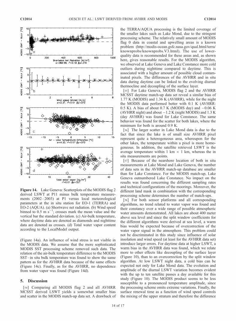
(Figure 14a). An influence of wind stress is not visible inthe MODIS data. We assume that the more sophisticatedMODIS SST processing scheme removed such data. Therelation of the air-bulk temperature difference to the MODISSST–in situ bulk temperature was found to show the samepattern as for the AVHRR data because of the same effects(Figure 14c). Finally, as for the AVHRR, no dependencefrom water vapor was found (Figure 14d).

5. Discussion

[54] Comparing all MODIS flag 2 and all AVHRRMCSST derived LSWT yields a somewhat smaller biasand scatter in the MODIS match-up data set. A drawback of

the TERRA/AQUA processing is the limited coverage ofthe smaller lakes such as Lake Mond, due to the stringentprocessing scheme. The relatively small amount of MODISflag 0 data in coastal and upwelling areas is a knownproblem (http://modis-ocean.gsfc.nasa.gov/qual.html/terra/knownprobs/knownprobs.V3.html). The use of lower-quality data is recommended for these areas and, as shownhere, gives reasonable results. For the MODIS algorithm,we observed at Lake Geneva and Lake Constance more coldoutliers during nighttime compared to daytime. This isassociated with a higher amount of possible cloud contam-inated pixels. The differences of the AVHRR and in situdata during daytime can be linked to the evolving diurnalthermocline and decoupling of the surface layer.[55] For Lake Geneva, MODIS flag 2 and the AVHRR

MCSST daytime match-up data set reveal a similar bias of1.77 K (MODIS) and 1.36 K (AVHRR), while for the nightthe MODIS data performed better with 0.1 K (AVHRR:0.5 K). A bias of about 0.7 K (MODIS day) and �0.06 K(AVHRR night) and about�1.2 K (night MODIS) and 1.3 K(day AVHRR) was found for Lake Constance. The samebehavior was found for the scatter for both lakes, where theminimum for both is around 0.9 K.[56] The larger scatter in Lake Mond data is due to the

fact that since the lake is of small size AVHRR pixelrepresent quite a heterogeneous area, whereupon for theother lakes, the temperature within a pixel is more homo-geneous. In addition, the satellite retrieved LSWT is theaverage temperature within 1 km � 1 km, whereas the insitu measurements are points.[57] Because of the nearshore location of both in situ

measurements at Lake Mond and Lake Geneva, the numberof data sets in the AVHRR match-up database are smallerthan for Lake Constance. For the MODIS match-up, LakeGeneva outnumbered Lake Constance. No impact on theresults was found concerning the different sampling ratesand technical configurations of the moorings. Moreover, thedifferent land mask in combination with the correspondingprocessing scheme determines the number of match-ups.[58] For both sensor platforms and all corresponding

algorithms, no trend related to water vapor was found andtheir constancy over a wide range of possible atmosphericwater amounts demonstrated. All lakes are about 400 meterabove sea level and since the split window coefficients forthe different algorithms were derived at sea level, a warmbias would be expected because of overcorrection of thewater vapor signal in the atmosphere. This problem couldnot be discriminated in this study since influence of solarinsolation and wind speed (at least for the AVHRR data set)introduce larger errors. For daytime data at higher LSWT, awarm bias in the AVHRR data was found, which we relatemore to other effects like decoupling of the surface layer(Figure 10), than to an overcorrection by the split windowalgorithm. At low LSWT night data, a cold bias can beexpected not only for Lake Mond data. The evolution andamplitude of the diurnal LSWT variation becomes evidentwith the up to ten satellite passes a day available for thisstudy (Figure 10). The MODIS product seems to be lesssusceptible to a pronounced temperature amplitude, sincethe processing scheme omits extreme variations. Finally, thesurface renewal time as a function of wind speed controlsthe mixing of the upper stratum and therefore the difference

Figure 14. Lake Geneva: Scatterplots of the MODIS flag 2derived LSWT at P11 minus bulk temperature measure-ments (2002–2003) at P1 versus local meteorologicalparameters at the in situ station for EO-1 (TERRA) andEO-2 (AQUA). (a) Shortwave net radiation. (b) Wind speedbinned to 0.5 m s�1; crosses mark the mean value and thevertical bar the standard deviation. (c) Air-bulk temperature,where daytime data are denoted as diamonds and nighttimedata are denoted as crosses. (d) Total water vapor contentaccording to the LocalModel output.


14 of 17

C12014

between bulk and LSWT. At low wind speed situations, asthey often occur over alpine lakes, we have to expect alarger difference.

6. Conclusion

[59] In this study, we ascertain the capability and limi-tations of the various AVHRR and the two MODIS sensorsto derive LSWT for three lakes with an areal extent rangingfrom 584 km2 to less than 14 km2, covering a time period of2 years. The LSWT validation revealed that for AVHRR,the MCSST algorithm is more accurate than the nonlinearapproach. This is could be expected, since the NLSST wasoriginally introduced to improve results in regions of highwater vapor. In general, daylight LSWT temperatures,especially in summer, tend to have a warmer bias comparedto the in situ data. Whereas at night we observed a smallerbias which becomes a cold bias at lower LSWTs especiallyin the case of Lake Mond. For the NOAA operatedsatellites, NOAA 16 MCSST night passes of Lake Genevagive the best results (bias, 0.18 K and standard deviation,0.73 K). The different accuracy results for the varioussatellites with comparable sensors can be related to sensornoise, except for the larger offset of NOAA 12: the MCSST/NLSST coefficients cannot be considered operational andmight be out of date. The good results of the non opera-tional NOAA 15 could be considered rather fortuitous; thereis even some potential to improve results for this sensor,using more recent coefficients. For the MODIS product,best results were found for TERRA nighttime data (bias,�0.08 K and standard deviation, 0.92 K). We suggest to useflag 2 data, since it includes most of the lake pixels, even ifthey are probably cloud contaminated.[60] Comparing the Lake Geneva and Lake Constance

data set of MODIS flag 2 and AVHRR MCSST similarscatter was found, ranging from 0.9 to 1.6 K. The bias forMODIS was within the range of �1.73–1.9 K, whereas forAVHRR �0.28–1.5 K. This is about 0.6 K higher than theresults by Li et al. [2001] for the Great Lakes using theAVHRR.[61] Lake Mond with the size of 15 km2 is not covered by

any MODIS data set with a useful amount of data points.Using AVHRR, we have to deal with a higher bias andscatter compared to the other lakes.[62] Since for nighttime data the effect of the diurnal

thermocline/decoupling of the top surface water is small,such data gives more reliable results than daytime AVHRRimagery.[63] The consistent agreement of the proposed LSWT

retrieval scheme with different data sets well establishedamong the limnological community proves for the first timethe applicability of LSWT for lake studies. Concerning thefindings shown in this study, AVHRR becomes a powerfultool for building up a lake climatology with its more than20 years of coverage. Although larger errors are foundcompared to open ocean retrievals, both MODIS andAVHRR are well suited for near-realtime thermal lakemonitoring, or for assimilation into high-resolution numer-ical weather prediction models. The spatial and temporalcoverage accounts for the lower absolute accuracy.[64] A novelty shown in this study is the observation of

the diurnal lake water surface temperature amplitude by the

different sensors. For the first time, advantage has beentaken of the current orbital configuration of the NOAAoperated and MODIS platforms for the description of thisprocess. It could be clearly shown that the radiometricallymeasured surface water temperature can be significantlymore strongly influenced by the prevailing regime thanby the underlying bulk temperature. The damped mixingfound for a typical calm day with clear sky regime isdifferent from open ocean conditions. These findings havepotentially interesting implication for the future of remotesensing of water surface temperatures in lakes and openocean.

[65] Acknowledgments. The authors are grateful to the threeanonymous reviewers for their very valuable remarks and comments.We would like to thank Claude Perrinjaquet (ENAC-LHE EPFL), FrankPeeters (University of Konstanz), and Martin Dokulil (Institute forLimnology, Mondsee) for providing in situ temperature data for LakeGeneva, Lake Constance, and Lake Mond, respectively. Our thanks go toMeteoSwiss for supplying meteorological data. This study has beenfunded by the MeteoSwiss and the Swiss Defense Procurement Agency.Support by the Stiftung Marchese Francesco Medici del Vascello isgratefully acknowledged.

ReferencesArnell, N., B. Bates, H. Lang, J. Magnuson, and P. Mulholland (1996),Hydrology and freshwater ecology, Climate Change 1995: Impacts,Adaptations, and Mitigation—Scientific-Technical Analysis, pp. 325–363, Cambridge Univ. Press, New York.

Barton, I. J., and A. J. Prata (1995), Satellite derived sea surface tem-perature data sets for climate applications, Adv. Space Res., 16(10),127–136.

Boehm, E., S. Marullo, and R. Santoleri (1991), AVHRR visible-IR detec-tion of diurnal warming events in the western Mediterranean Sea, Int.J. Remote Sens., 12, 695–701.

Brown, O., and P. Minnett (1999), MODIS infrared sea surface temperaturealgorithm, in Algorithm Theoretical Basis Document Version 2, Univ. ofMiami, Miami, Fla.

Bussieres, N., D. Verseghy, and J. I. MacPherson (2001), The evolution ofAVHRR-derived water temperatures over boreal lakes, Remote Sens.Environ., 80, 373–384.

Cornillon, P., and L. Stramma (1998), The distribution of diurnal sea sur-face warming events in the western Sargasso Sea, J. Geophys. Res., 98,11,811–11,815.

Cracknell, A.P. (1997), The Advanced Very High Resolution Radiometer(AVHRR), Taylor and Francis, Philadelphia, Pa.

Di Vittorio, A. V., and W. J. Emery (2002), An automated, dynamic thresh-old cloud-masking algorithm for daytime AVHRR images over land,IEEE Trans. Geosci. Remote Sens., 40, 1682–1694.

Doms, G., and U. Schattler (2002), A description of the nonhydrostaticregional model LM. part I: Dynamics and numeric, technical report,Dts. Wetterdienst, Offenbach, Germany.

Donlon, C., P. Minnett, C. Gentemann, T. Nightingale, I. Barton, B. Ward,and M. Murray (2002), Toward improved validation of satellite sea sur-face skin temperature measurements for climate research, J. Clim., 15,353–369.

Emery, W. J., S. Castro, G. A. Wick, P. Schluessel, and C. Donlon(2001), Estimating sea surface temperature from infrared satelliteand in situ temperature data, Bull. Am. Meterol. Soc., 82, 2773–2786.

Esaias, W. E., et al. (1998), An overview of MODIS capabilities for oceanscience observations, IEEE Trans. Geosci. Remote Sens., 36, 1250–1265.

Fairall, C. W., E. F. Bradley, J. S. Godfrey, G. A. Wick, J. B. Edson, andG. S. Young (1996), Cool-skin and warm-layer effects on sea surfacetemperature, J. Geophys. Res., 101, 1295–1308.

Fer, I., U. Lemmin, and S. A. Thorpe (2001), Cascading of water down thesloping sides of a deep lake in winter, Geophys. Res. Lett., 28, 2093–2096.

Fer, I., U. Lemmin, and S. A. Thorpe (2002), Observations of mixingnear the sides of a deep lake in winter, Limnol. Oceanogr., 47, 535–544.

Gentemann, C. L., C. J. Donlon, A. Stuart-Menteth, and F. Wentz (2003),Diurnal signals in satellite sea surface temperature measurements, Geo-phys. Res. Lett., 30(3), 1140, doi:10.1029/2002GL016291.


15 of 17

C12014

Goodrum, G., K. B. Kidwell, and W. Winston (2000), NOAA KLM user’sguide, technical report, Natl. Oceanic and Atmos. Admin., Silver Spring,Md.

Hasse, L., and S. D. Smith (1997), Local sea surface wind, wind stress, andsensible and latent heat fluxes, J. Clim., 10, 2711–2724.

Hawkins, J. D., R. M. Clancy, and J. F. Price (1993), Use of AVHRR data toverify a system for forecasting diurnal sea surface temperature variability,Int. J. Remote Sens., 14, 1347–1357.

Hook, S., F. Prata, R. Alley, A. Abtahi, R. Richards, S. Schladow, andS. Palmarsson (2003), Retrieval of lake bulk and skin temperaturesusing Along-Track Scanning Radiometer (ATSR-2) data: A case studyusing Lake Tahoe, California, J. Atmos. Oceanic Technol., 20, 534–548.

Hussey, J. (1985), ENVIROSAT—2000 report NOAA satellite require-ments forecast, technical report, Natl. Oceanic and Atmos. Admin., SilverSpring, Md.

Ignatov, A., and G. Gutman (1999), Monthly mean diurnal cycles in surfacetemperatures over land for global climate studies, J. Clim., 12, 1900–1910.

Ignatov, A., I. Laszlo, E. Harrod, K. Kidwell, and G. Goodrum (2004),Equator crossing times for NOAA, ERS and EOS Sun-synchronoussatellites, Int. J. Remote Sens., 25(23), 5255 – 5266, doi:10.1080/01431160410001712981.

Imberger, J., and J. C. Patterson (1990), Physical limnology, Adv. Appl.Mech., 27, 303–475.

Katsaros, K. B. (1977), Sea-surface temperature deviation at very low windspeeds—Is there a limit?, Tellus, 29, 229–239.

Katsaros, K. B., W. T. Liu, A. Businger, and J. E. Tillman (1977), Heat-transport and thermal structure in interfacial boundary-layer measured inan open tank of water in turbulent free convection, J. Fluid Mech., 83,311–335.

Kearns, E. J., R. H. Hanafin, P. Evans, and O. B. Brown (2000), Anindependent assessment of pathfinder AVHRR sea surface temperatureaccuracy using the Marine Atmosphere Emitted Radiance Interferometer(MAERI), Bull. Am. Meterol. Soc., 81, 1525–1536.

Key, J. (2002), The Cloud and Surface Parameter Retrieval (CASPR)System for Polar AVHRR—User’s Guide, Coop. Inst. for Meteorol.Sat. Stud., Univ. of Wis., Madison. (Available at http://stratus.ssec.wisc.edu.)

Khattak, S., R. Vaughan, and A. Cracknell (1991), Sunglint and itsobservation in AVHRR data, Remote Sens. Environ., 37, 101–116.

Kidwell, K. (1998), NOAA polar orbiter data user’s guide (TIROS-N,NOAA-6, -7, -8, -9,-10, -11, -12, -13 and -14), technical report, Natl.Oceanic and Atmos. Admin., Silver Spring, Md.

Kilpatrick, K. A., G. P. Podesta, and R. Evans (2001), Overview ofthe NOAA/NASA advanced very high resolution radiometer Pathfinderalgorithm for sea surface temperature and associated matchup database,J. Geophys. Res., 106, 9179–9198.

King, M. D., D. D. Herring, and D. J. Diner (1995), Earth observingsystem: A space-based program for assessing mankind’s impact on theglobal environment, Opt. Photonic News, 6, 34–39.

Li, X., W. Pichel, P. Clemente-Colon, V. Krasnopolsky, and J. Sapper(2001), Validation of coastal sea and lake surface temperature measure-ments derived from NOAA/AVHRR data, Int. J. Remote Sens., 22,1285–1303.

Livingstone, D. M., and M. T. Dokulil (2001), Eighty years of spatiallycoherent Austrian lake surface temperatures and their relationship toregional air temperature and the North Atlantic Oscillation, Limnol.Oceanogr., 46, 1220–1227.

McClain, E., W. Pichel, and C. Walton (1985), Comparative performance ofAVHRR-based multichannel sea surface temperatures, J. Geophys. Res.,90, 11,587–11,601.

Minnett, P. J. (1991), Consequences of sea surface temperature variabilityon the validation and applications of satellite measurements, J. Geophys.Res., 96, 18,475–18,489.

Minnett, P. (2003), Radiometric measurements of the sea-surface skin tem-perature: The competing roles of the diurnal thermocline and the coolskin, Int. J. Remote Sens., 24, 5033–5047.

Minnett, P. J., R. O. Knuteson, F. A. Best, B. J. Osborne, J. A. Hanafin, andO. B. Brown (2001), The Marine-Atmospheric Emitted Radiance Inter-ferometer: A High-Accuracy, Seagoing Infrared Spectroradiometer,J. Atmos. Oceanic Technol., 18, 994–1013.

Minnett, P. J., R. H. Evans, E. Kearns, and O. B. Brown (2002), Sea-surfacetemperature measured by the Moderate Resolution Imaging Spectro-radiometer (MODIS), in Remote Sensing: Integrating Our View of thePlanet, vol. 2, edited by E. F. LeDrew, pp. 1177–1179, Inst. of Electr.and Electr. Eng., New York.

Monismith, S. G. (1985), Wind-forces motion in stratified lakes and theireffect on mixed layer shear, Limnol. Oceanogr., 30, 771–783.

Monismith, S. G. (1986), An experimental study of the upwelling responseof stratified reservoirs to surface shear stress, J. Fluid Mech., 171, 407–439.

Mortimer, C. H. (1952), Water movements in lakes during summer strati-fication: Evidence from distribution of temperature in Windmere, Philos.Trans. R. Soc. London, Ser. B, 236, 355–404.

Murray, M. J., M. R. Allen, C. J. Merchant, A. R. Harris, and C. J. Donlon(2000), Direct observations of skin-bulk SST variability, Geophys. Res.Lett., 27, 1171–1174.

Prabhakara, C., R. Fraser, G. Dalu, M.-L. C. Wu, R. Curran, and T. Styles(1988), Thin cirrus clouds: Seasonal distribution over oceans deducedfrom Nimbus-4 IRIS, J. Appl. Meteorol., 27, 379–399.

Price, J. C. (1991), Timing of NOAA afternoon passes, Int. J. Remote Sens.,12, 193–198.

Rao, C., J. Sullivan, C. Walton, J. Brown, and R. Evans (1993), Nonlinear-ity corrections for the thermal infrared channels of the Advanced VeryHigh Resolution Radiometer: Assessment and recommendations, NOAATech. Rep., NESDIS 69, Gov. Print. Off., Washington, D. C.

Rao, P. K. (1990), Weather Satellites: Systems, Data and EnvironmentalApplications, Am. Meteorol. Soc., Boston, Mass.

Reynolds, R. W., and T.-M. Smith (1994), Improved global sea surfacetemperature analyses using optimum interpolation, J. Clim., 7, 929-48.

Robinson, I., and C. Donlon (2003), Global measurement of sea surfacetemperature from space: Some new perspectives, Global Atmos. OceanSyst., 9, 19–37.

Robinson, I., N. Wells, and H. Charnock (1984), The sea surface thermalboundary layers and its relevance to the measurement of sea surfacetemperature by airborne and space borne radiometers, Int. J. RemoteSens., 95, 13,341–13,356.

Salomonson, V., W. Barnes, P. Maymon, H. Montgomery, and H. Ostrow(1989), MODIS: Advanced facility instrument for studies of the Earth asa system, IEEE Trans. Geosci. Remote Sens., 27, 145–153.

Schluessel, P., H. Y. Shin, W. Emery, and H. Grassl (1987), Comparison ofsatellite-derived sea surface temperatures with in situ skin measurements,J. Geophys. Res., 92, 2859–2874.

Schluessel, P., W. Emery, H. Grassl, and T. Mammen (1990), On the bulk-skin temperature difference and its impact on satellite remote sensing ofsea surface temperature, J. Geophys. Res., 95, 3341–3356.

Schraff, C., and R. Hess (2003), A description of the nonydrostatic regionalmodel LM. Part III: Data assimilation, technical report, Dtsch., Offen-bach, Germany.

Schwab, D. J., G. A. Leshkevich, and G. C. Muhr (1992), Satellite mea-surements of surface water temperature in the great lakes: Great lakescoastwatch, J. Great Lakes Res., 18, 247–258.

Schwab, D. J., G. A. Leshkevich, and G. C. Muhr (1999), Automatedmapping of surface water temperature in the Great Lakes, J. Great LakesRes., 25, 468–481.

Simpson, J. J., and J. R. Stitt (1998), A procedure for the detection andremoval of cloud shadow from AVHRR data over land, IEEE Trans.Geosci. Remote Sens., 36, 880–897.

Soloviev, A. V., and P. Schlussel (1997), Evolution of cool skin and directair-sea gas transfer coefficient during daytime, Boundary Layer Meteorol.,77, 45–68.

Strub, P. T., and T. Powell (1986), Wind-driven surface transport in strati-fied closed basins: Direct versus residual calculation, J. Geophys. Res.,91, 8497–8508.

Strub, P. T., and T. Powell (1987), Surface temperature and transport inLake Tahoe: Inferences from satellite (AVHRR) imagery, Cont. ShelfRes., 7, 1001–1013.

Thiemann, S., and H. Schiller (2003), Determination of the bulk tempera-ture from NOAA/AVHRR satellite data in a midlatitude lake, Int. J. Appl.Earth Obs. Geoinf., 4, 339–349.

Walton, C. C. (1988), Nonlinear multichannel algorithms for estimating seasurface temperature with AVHRR satellite data, J. Appl. Meteorol., 27,115–124.

Walton, C. C., W. G. Pichel, J. F. Sapper, and D. May (1998a), Thedevelopment and operational application of nonlinear algorithms forthe measurement of sea surface temperatures with the NOAA polar-orbiting environmental satellites, J. Geophys. Res., 103, 27,999–28,012.

Walton, C. C., J. T. Sullivan, C. R. N. Rao, and M. Weinreb (1998b),Corrections for detector nonlinearities and calibration inconsistencies ofthe infrared channels of the advanced very high resolution radiometer,J. Geophys. Res., 103, 3323–3337.

Wessel, P., and W. H. F. Smith (1996), A global, self-consistent, hierarch-ical, high-resolution shoreline database, J. Geophys. Res., 101, 8741–8743.

Wick, G. A., and J. J. Bates (2002), Satellite and skin-layer effects onthe accuracy of sea surface temperature measurements from the GOESsatellites, J. Atmos. Oceanic Technol., 19, 1834–1848.


16 of 17

C12014

Wick, G. A., W. J. Emery, L. H. Kantha, and P. Schlossel (1996), Thebehavior of the bulk-skin sea surface temperature difference undervarying wind speed and heat flux, J. Phys. Oceanogr., 26, 1969–1988.

Wooster, M., G. Patterson, R. Loftie, and C. Sear (2001), Derivation andvalidation of the seasonal thermal structure of Lake Malawi usingmulti-satellite AVHRR observations, Int. J. Remote Sens., 22, 2953–2972.

Wu, X., and W. L. Smith (1997), Emissivity of rough sea surface for 8-13 mm: modeling and verification, Appl. Opt., 36, 2609–2619.

Yokoyama, R., S. Tanba, and T. Souma (1993), Air-sea interacting effects tothe sea surface temperature observation by NOAA/AVHRR, Int. J. Re-mote Sens., 14, 2631–2646.

��A. Hauser, D. C. Oesch, and S. Wunderle, Department of Geography,

University of Bern, Hallerstrasse 12, CH-3012 Bern, Switzerland.([email protected])J.-M. Jaquet, Earth Observation Unit, UNEP-DEWA-GRID/University of

Geneva, CH-1205 Geneva, Switzerland.


17 of 17

C12014

lake surface water temperature retrieval using ... - unep · moderate resolution imaging...

Documents