moderate resolution imaging spectroradiometer (modis...
TRANSCRIPT
JPL Publication 12-17
Moderate Resolution Imaging
Spectroradiometer (MODIS) MOD21 Land
Surface Temperature and Emissivity
Algorithm Theoretical Basis Document
G. Hulley
S. Hook
T. Hughes
Jet Propulsion Laboratory
National Aeronautics and
Space Administration
Jet Propulsion Laboratory
California Institute of Technology
Pasadena, California
August 2012

MODIS MOD21 LAND SURFACE TEMPERATURE AND EMISSIVITY ATBD
This research was carried out at the Jet Propulsion Laboratory, California Institute of Technology, under a
contract with the National Aeronautics and Space Administration.
Reference herein to any specific commercial product, process, or service by trade name, trademark,
manufacturer, or otherwise, does not constitute or imply its endorsement by the United States
Government or the Jet Propulsion Laboratory, California Institute of Technology.
© 2012. California Institute of Technology. Government sponsorship acknowledged.
MODIS MOD21 LAND SURFACE TEMPERATURE AND EMISSIVITY ATBD
Revisions:
08/17/2012: Version 1.0 draft by Glynn Hulley
11/02/12: Section 10: Validation, updated by Glynn Hulley
11/19/2012: Edited by Peter Basch, Technical Editor/Writer, Jet Propulsion Laboratory
03/27/2014: Updated Table 2 to correct an error in the calculation of sky irradiance
coefficients. Updated Table 3 and 4 WVS and bmp coefficients which are now valid for view
angles up to 65 degrees and for a more diverse set of global atmospheric conditions.
Reviews:
MODIS MOD21 LAND SURFACE TEMPERATURE AND EMISSIVITY ATBD
2
Contacts
Readers seeking additional information about this study may contact the following researchers:
Glynn C. Hulley
MS 183-501
Jet Propulsion Laboratory
4800 Oak Grove Dr.
Pasadena, CA 91109
Email: [email protected]
Office: (818) 354-2979
Simon J. Hook
MS 183-501
Jet Propulsion Laboratory
4800 Oak Grove Dr.
Pasadena, CA 91109
Email: [email protected]
Office: (818) 354-0974
MODIS MOD21 LAND SURFACE TEMPERATURE AND EMISSIVITY ATBD
3
Contents
Contacts ......................................................................................................................................... 2
1 Introduction .......................................................................................................................... 8
2 MODIS Background .......................................................................................................... 10 2.1 Calibration................................................................................................................... 10 2.2 Instrument Characteristics .......................................................................................... 11 2.3 LST&E Standard Products .......................................................................................... 11
3 Earth Science Relevance .................................................................................................... 14 3.1 Use of LST&E in Climate/Ecosystem Models ........................................................... 14
3.2 Use of LST&E in Cryospheric Research .................................................................... 15 3.3 Use of LST&E in Atmospheric Retrieval Schemes .................................................... 16
4 Atmospheric Correction .................................................................................................... 17 4.1 Thermal Infrared Radiance ......................................................................................... 17
4.2 Emissivity ................................................................................................................... 21 4.3 Radiative Transfer Model ........................................................................................... 21
4.4 Atmospheric Profiles .................................................................................................. 22 4.5 Radiative Transfer Sensitivity Analysis ...................................................................... 24
5 Water Vapor Scaling Method ........................................................................................... 26 5.1 Gray Pixel Computation ............................................................................................. 27 5.2 Interpolation and Smoothing....................................................................................... 29
5.3 Scaling Atmospheric Parameters ................................................................................ 31 5.3.1 Transmittance and Path Radiance .................................................................... 31 5.3.2 Downward Sky Irradiance ................................................................................ 31
5.4 Calculating the EMC/WVD Coefficients ................................................................... 32
6 Temperature and Emissivity Separation Approaches .................................................... 35 6.1 Deterministic Approaches ........................................................................................... 35
6.1.1 SW Algorithms ................................................................................................. 35
6.1.2 Single-Band Inversion ...................................................................................... 37 6.1.3 Non-deterministic Approaches ......................................................................... 37
6.2 TES Algorithm ............................................................................................................ 40 6.2.1 TES Data Inputs ............................................................................................... 40 6.2.2 TES Limitations ............................................................................................... 41 6.2.3 TES Processing Flow ....................................................................................... 42 6.2.4 NEM Module .................................................................................................... 45
6.2.5 Subtracting Downwelling Sky Irradiance ........................................................ 45
6.2.6 Refinement of ........................................................................................ 46 6.2.7 Ratio Module .................................................................................................... 47 6.2.8 MMD Module ................................................................................................... 47
6.2.9 MMD vs. Regression ............................................................................. 50
6.2.10 Atmospheric Effects ......................................................................................... 52
7 Advantages of TES over SW approaches ........................................................................ 53 7.1 Land Cover Misclassification ..................................................................................... 54
MODIS MOD21 LAND SURFACE TEMPERATURE AND EMISSIVITY ATBD
4
7.2 Emissivity Error within Cover Type ........................................................................... 55
7.3 Soil Moisture Effects .................................................................................................. 56
8 Quality Assessment and Diagnostics ................................................................................ 57
9 Uncertainty Analysis .......................................................................................................... 60 9.1 The Temperature and Emissivity Uncertainty Simulator ........................................... 60 9.2 Atmospheric Profiles .................................................................................................. 61 9.3 Radiative Transfer Model ........................................................................................... 61 9.4 Surface End-Member Selection .................................................................................. 61 9.5 Radiative Transfer Simulations................................................................................... 62
9.6 Error Propagation ........................................................................................................ 64 9.7 Parameterization of Uncertainties ............................................................................... 67
10 Validation............................................................................................................................ 70 10.1 Water Sites .................................................................................................................. 71 10.2 Vegetated Sites............................................................................................................ 72 10.3 Pseudo-invariant Sand Dune Sites .............................................................................. 73
10.3.1 Emissivity Validation ....................................................................................... 74 10.3.2 LST Validation ................................................................................................. 76
11 References ........................................................................................................................... 80

MODIS MOD21 LAND SURFACE TEMPERATURE AND EMISSIVITY ATBD
5
Figures
Figure 1. Simulated atmospheric transmittance for a US Standard Atmosphere (red) and tropical atmosphere (blue)
in the 3–12 µm region. Also shown is the solar irradiance contribution W/m2/µm
2. ....................................... 18
Figure 2. Radiance simulations of the surface-emitted radiance, surface-emitted and reflected radiance, and at-sensor
radiance using the MODTRAN 5.2 radiative transfer code, US Standard Atmosphere, quartz emissivity
spectrum, surface temperature = 300 K, and viewing angle set to nadir. Vertical bars show placements of
the MODIS TIR bands 29 (8.55 µm), 31 (11 µm), and 32 (12 µm). ............................................................... 19 Figure 3. MODIS spectral response functions for bands 29 (red), 31 (green), and 32 (blue) plotted with a typical
transmittance curve for a mid-latitude summer atmosphere. ........................................................................... 20 Figure 4. Bias and RMS differences between Aqua MODIS MOD07, AIRS v4 operational temperature and moisture
profiles and the “best estimate of the atmosphere” (Tobin et al. 2006) dataset for 80 clear sky cases over
the SGP ARM site. From Seemann et al. (2006). ............................................................................................ 24 Figure 5. Clockwise from top left: Google Earth visible image; first guess gray-pixel map; TLR refinement; and
final gray pixel map for a MODIS scene cutout over parts of Arizona and southeastern California
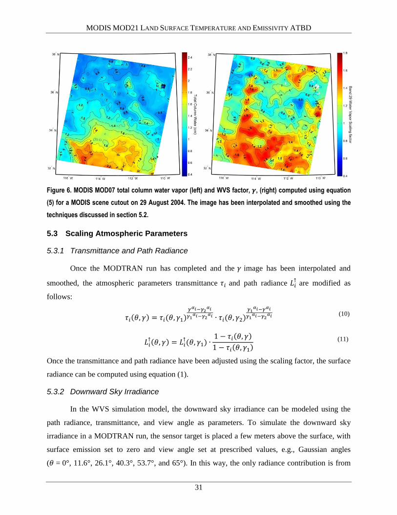
(black = graybody, white = bare) on 29 August 2004. See text for details. ..................................................... 29 Figure 6. MODIS MOD07 total column water vapor (left) and WVS factor, , (right) computed using equation (5)
for a MODIS scene cutout on 29 August 2004. The image has been interpolated and smoothed using the
techniques discussed in section 5.2. ................................................................................................................. 31 Figure 7. Comparisons between the atmospheric transmittance (top), path radiance (W/m
2/µm
1) (middle), and
computed surface radiance (W/m2/µm
1) (bottom), before and after applying the WVS scaling factor to a
MODIS scene cutout shown in Figure 5. Results are shown for MODIS band 29 (8.55 µm). ........................ 33 Figure 8. ASTER (left panels) and MODIS (right panels) LST uncertainty distributions plotted versus TCW and
simulated LST for all end-member surface types (graybody, soils, sands, and rocks), for the TES algorithm
including atmospheric error (TES+atm) and with the WVS method applied (TES+atm+wvs). ...................... 42 Figure 9. Flow diagram showing all steps in the retrieval process in generating the MODIS MOD21 LST&E product
starting with TIR at-sensor radiances and progressing through atmospheric correction, cloud detection, and
the TES algorithm. ........................................................................................................................................... 43 Figure 10. Flow diagram of the TES algorithm in its entirety, including the NEM, RATIO, and MMD modules.
Details are included in the text, including information about the refinement of . ................................. 44 Figure 11. Clockwise from top left: MODIS cutouts of land surface emissivity for band 29 (8.55 µm); band 31 (11
µm), surface temperature (K) and band 32 emissivity (12 µm); output from the TES algorithm over the
Imperial Valley, southeastern California on 29 August 2004. ......................................................................... 49 Figure 12. MODIS derived TES and NEM emissivity spectra for three different surface types for the MODIS cutout
shown in Figure 11: Algodones Dunes, Salton Sea, and shrublands (mixed soil and vegetation). Details of
the TES and NEM outputs from these spectra are shown in Table 5. .............................................................. 49 Figure 13. MODIS and ASTER calibration curves of minimum emissivity vs. MMD. The lab data (crosses) are
computed from 150 spectra consisting of a broad range of terrestrial materials (rocks, sand, soil, water,
vegetation, and ice). ......................................................................................................................................... 51 Figure 14. Emissivity spectra comparisons on June 15, 2000 over the Salton Sea between ASTER (3-band), ASTER
(5-band), and MODTES, using the TES algorithm along with lab spectra of water from the ASTER
spectral library. Results from the WVS method and the STD atmospheric correction are also shown. An
estimate of the PWV from the MOD07 atmospheric product indicates very high humidity on this day. ........ 53 Figure 15. Emissivity images (left) and surface temperature images (right) for ASTER (top), MODIS TES
(MODTES) (center) and MODIS SW (MOD11_L2) (bottom) products over the Station Fire burn scar just
north of Pasadena, CA. Location of JPL in Pasadena and burn scar area indicated at top right. MODTES
and ASTER results match closely; however, the MOD11_L2 temperatures are underestimated by as much
as 12 K, due to an incorrect emissivity classification. ..................................................................................... 55 Figure 16. (left) ASTER band 12 (9.1 µm) emissivity image over Mauna Loa caldera, Hawaii on 5 June 2000, and
(right) emissivity spectra from ASTER, MODTES, and MOD11 emissivity classification. While ASTER
and MODTES agree closely, MOD11 emissivities are too high, resulting in large LST discrepancies
between MODTES and MOD1 (12 K) due to misclassification in bands 31 (11 µm) and 32 (12 µm). .......... 56 Figure 17. (top) Emissivity variation for a rainfall event over the Namib desert showing results from MOD11B1 v4
(day/night algorithm), MOD11_L2 (SW), and MODIS TES (MODTES). (bottom) Corresponding soil
MODIS MOD21 LAND SURFACE TEMPERATURE AND EMISSIVITY ATBD
6
moisture variation from AMSRE-E and rainfall estimates from the Tropical Rainfall Measuring Mission
(TRMM). It is clear that the physical retrievals, show increases in emissivity due to soil moisture, whereas
the SW values are held constant throughout the rainfall period from 15–21 April. From Hulley et al.
(2010). .............................................................................................................................................................. 57 Figure 18. MODIS LST uncertainties using the TES algorithm versus TCW for four viewing Gaussian angles of 0°,
26.1°, 40.3°, and 53.7°. The value n represents the number of data points used for a specific land surface
type, in this case bare surfaces (rocks, soils, sands). ........................................................................................ 66 Figure 19. MODIS TES retrievals including WVS correction over the southwestern United States on 7 August 2004:
(a) (top left) LST, (b) (top right) emissivity for band 29 (8.55 µm), (c) (bottom left) LST uncertainty, and
(d) (bottom right) emissivity uncertainty for band 29 (8.55 µm). White areas over land indicate areas of
cloud that have been masked out using the MOD35 cloud mask product. ...................................................... 69 Figure 20. Difference between the MODIS (MOD11_L2) and ASTER (AST08) LST products and in-situ
measurements at Lake Tahoe. The MODIS product is accurate to ±0.2 K, while the ASTER product has a
bias of 1 K due to residual atmospheric correction effects. ............................................................................. 72 Figure 21. Laboratory-measured emissivity spectra of sand samples collected at ten pseudo-invariant sand dune
validation sites in the southwestern United States. The sites cover a wide range of emissivities in the TIR
region. .............................................................................................................................................................. 75 Figure 22. ASTER false-color visible images (top) and emissivity spectra comparisons between ASTER TES and
lab results for Algodones Dunes, California; White Sands, New Mexico; and Great Sands, Colorado
(bottom). Squares with blue dots indicate the sampling areas. ASTER error bars show temporal and spatial
variation, whereas lab spectra show spatial variation. ..................................................................................... 75 Figure 23. An example of the R-based validation method applied to the MODIS Aqua MOD11 and MOD21 LST
products over six pseudo-invariant sand dune sites using all data during 2005. AIRS profiles and lab-
measured emissivities from samples collected at the sites were used for the R-based calculations. ............... 79
MODIS MOD21 LAND SURFACE TEMPERATURE AND EMISSIVITY ATBD
7
Tables
Table 1. Percent changes in simulated at-sensor radiances for changes in input geophysical parameters for MODIS
bands 29, 31, and 32, with equivalent change in brightness temperature in parentheses. ................................ 25 Table 2. MODIS-Terra regression coefficients for equation 13. ..................................................................................... 32 Table 3. MODIS-Terra EMC/WVD coefficients used in equation (5). ........................................................................... 34 Table 4. MODIS-Terra band model parameters in equation (6). .................................................................................... 34 Table 5. Output from various stages of the MODTES algorithm for three surface types: sand dunes, Salton Sea, and
shrubland transition zone for a MODIS test scene over the Imperial Valley, southeastern California. ........... 47 Table 6. Quality assurance (QA) data plane 1 description of the three data fields: data quality, cloud mask, and cloud
adjacency. ........................................................................................................................................................ 59 Table 7. Quality assurance (QA) data plane 2 description of output diagnostics from the TES algorithm. .................... 59 Table 8. The core set of global validation sites according to IGBP class to be used for validation and calibration of
the MODIS MOD21 land surface temperature and emissivity product. .......................................................... 71 Table 9. R-based LST validation statistics from six pseudo-invariant sand dune sites using all MOD11 and MOD21
LST retrievals during 2005. ............................................................................................................................. 78 Table 10. Emissivity comparisons between lab, MOD11, and MOD21 at six pseudo-invariant sand sites. ................... 78
MODIS MOD21 LAND SURFACE TEMPERATURE AND EMISSIVITY ATBD
8
1 Introduction
This document outlines the theory and methodology for generating the Moderate
Resolution Imaging Spectroradiometer (MODIS) Level-2 daily daytime and nighttime 1-km land
surface temperature (LST) and emissivity product using the Temperature Emissivity Separation
(TES) algorithm. The MODIS-TES (MOD21_L2) product, will include the LST and emissivity
for three MODIS thermal infrared (TIR) bands 29, 31, and 32, and will be generated for data
from the NASA-EOS AM and PM platforms. This is version 1.0 of the ATBD and the goal is
maintain a ‘living’ version of this document with changes made when necessary. The current
standard baseline MODIS LST products (MOD11*) are derived from the generalized split-
window (SW) algorithm (Wan and Dozier 1996), which produces a 1-km LST product and two
classification-based emissivities for bands 31 and 32; and a physics-based day/night algorithm
(Wan and Li 1997), which produces a 5-km (C4) and 6-km (C5) LST product and emissivity for
seven MODIS bands: 20, 22, 23, 29, 31–33.
The land surface temperature and emissivity (LST&E) are derived from the surface
radiance that is obtained by atmospherically correcting the at-sensor radiance. LST&E data are
used for many Earth surface related studies such as surface energy balance modeling (Zhou et al.
2003b) and land-cover land-use change detection (French et al. 2008), while they are also critical
for accurately retrieving important climate variables such as air temperature and relative
humidity (Yao et al. 2011). The LST is an important long-term climate indicator, and a key
variable for drought monitoring over arid lands (Anderson et al. 2011a; Rhee et al. 2010). The
LST is an input to ecological models that determine important variables used for water use
management such as evapotranspiration and soil moisture (Anderson et al. 2011b). Multispectral
emissivity retrievals are also important for Earth surface studies. For example, emissivity
spectral signatures are important for geologic studies and mineral mapping studies (Hook et al.
2005; Vaughan et al. 2005). This is because emissivity features in the TIR region are unique for
many different types of materials that make up the Earth’s surface, such as quartz, which is
ubiquitous in most of the arid regions of the world. Emissivities are also used for land use and
land cover change mapping since vegetation fractions can often be inferred if the background
soil is observable (French et al. 2008). Accurate knowledge of the surface emissivity is critical
MODIS MOD21 LAND SURFACE TEMPERATURE AND EMISSIVITY ATBD
9
for accurately recovering the LST, especially over land where emissivity variations can be large
both spectrally and spatially.
The MODTES algorithm derives its heritage from the ASTER TES algorithm (Gillespie
et al. 1998). ASTER is a five-channel multispectral TIR scanner that was launched on NASA’s
Terra spacecraft in December 1999 with a 90-m spatial resolution and revisit time of 16 days.
The MODTES LST&E products will be produced globally over all land cover types, excluding
open oceans for all cloud-free pixels. It is anticipated that the Level-2 products will be merged to
produce weekly, monthly, and seasonal products, with the monthly product most likely
producing global coverage, depending on cloud coverage. The generation of the higher level
merged products will be considered a project activity. The MODTES Level 2 products will be
initially inter-compared with the standard MOD11 products to identify regions and conditions for
divergence between the products, and validation will be accomplished using a combination of
temperature-based (T-based) and radiance-based (R-based) methods over dedicated field sites.
Maximum radiometric emission for the typical range of Earth surface temperatures,
excluding fires and volcanoes, is found in two infrared spectral “window” regions: the midwave
infrared (3.5–5 µm) and the thermal infrared (8–13 µm). The radiation emitted in these windows
for a given wavelength is a function of both temperature and emissivity. Determining the
separate contribution from each component in a radiometric measurement is an ill-posed problem
since there will always be more unknowns—N emissivities and a single temperature—than the
number of measurements, N, available. For MODIS, we will be solving for one temperature and
three emissivities (MODIS TIR bands 29, 31, and 32). To solve the ill-posed problem, an
additional constraint is needed, independent of the data. There have been numerous theories and
approaches over the past two decades to solve for this extra degree of freedom. For example, the
ASTER Temperature Emissivity Working Group (TEWG) analyzed ten different algorithms for
solving the problem (Gillespie et al. 1999). Most of these relied on a radiative transfer model to
correct at-sensor radiance to surface radiance and an emissivity model to separate temperature
and emissivity. Other approaches include the SW algorithm, which extends the sea-surface
temperature (SST) SW approach to land surfaces, assuming that land emissivities in the window
region (10.5–12 µm) are stable and well known. However, this assumption leads to unreasonably
large errors over barren regions where emissivities have large variations both spatially and
spectrally. The ASTER TEWG finally decided on a hybrid algorithm, termed the TES algorithm,
MODIS MOD21 LAND SURFACE TEMPERATURE AND EMISSIVITY ATBD
10
which capitalizes on the strengths of previous algorithms with additional features (Gillespie et al.
1998).
TES is applied to the land-leaving TIR radiances that are estimated by atmospherically
correcting the at-sensor radiance on a pixel-by-pixel basis using a radiative transfer model. TES
uses an empirical relationship to predict the minimum emissivity that would be observed from a
given spectral contrast, or minimum-maximum difference (MMD) (Kealy and Hook 1993;
Matsunaga 1994). The empirical relationship is referred to as the calibration curve and is derived
from a subset of spectra in the ASTER spectral library (Baldridge et al. 2009). A MODIS
calibration curve, applicable to MODIS TIR bands 29, 31, and 32 will be computed. Numerical
simulations have shown that TES is able to recover temperatures within 1.5 K and emissivities
within 0.015 for a wide range of surfaces and is a well-established physical algorithm that
produces seamless images with no artificial discontinuities such as might be seen in a land
classification type algorithm (Gillespie et al. 1998).
The remainder of the document will discuss the MODIS instrument characteristics,
provide a background on TIR remote sensing, give a full description and background on the TES
algorithm, provide quality assessment, discuss numerical simulation studies and uncertainty
analysis, and, finally, outline a validation plan.
2 MODIS Background
The MODIS sensors on NASA’s Terra (AM) and Aqua (PM) platforms are currently the
flagship instruments for global studies of Earth’s surface, atmosphere, cryosphere, and ocean
processes (Justice et al. 1998; Salomonson et al. 1989). In terms of LST&E products, the
strength of the MODIS is its ability to retrieve daily data at 1 km for both day- and nighttime
observations on a global scale.
2.1 Calibration
There are now multiple satellite sensors that measure the mid- and thermal infrared
radiance emitted from the Earth’s surface in multiple spectral channels. These sensors include
the Advanced Along Track Scanning Radiometer (AATSR), ASTER, Advanced Very High
Resolution Radiometer (AVHRR), and MODIS instruments. A satellite calibration
interconsistency study is currently underway for evaluating the interconsistency of these sensors
MODIS MOD21 LAND SURFACE TEMPERATURE AND EMISSIVITY ATBD
11
at the Lake Tahoe and Salton Sea cal/val sites. This effort has indicated that further work is
needed to consistently inter-calibrate the ATSR series and AVHRR series whereas ASTER and
MODIS have a clearly defined calibration and well-understood performance.
In-flight performance of TIR radiance data (3–14 µm) used in LST&E products is
typically determined through comparison with ground validation sites. Well-established
automated validation sites at Lake Tahoe, CA/NV, and Salton Sea, CA have been used to
validate the TIR data from numerous sensors including ASTER and MODIS (Hook et al. 2007).
Results from this work demonstrate that the MODIS (Terra and Aqua) instruments have met
their required radiometric calibration accuracy of 0.5–1% in the TIR bands used to retrieve
LST&E with differences of ±0.25% (~0.16K) for the lifetime of the missions. Similar work for
ASTER indicates its performance also meets the 1% requirements, provided additional steps are
taken to account for drift between calibrations (Tonooka et al. 2005).
2.2 Instrument Characteristics
The MODIS instrument acquires data in 36 spectral channels in the visible, near infrared,
and infrared wavelengths. Infrared channels 20, 22, 23, 29, 31, and 32 are centered on 3.79, 3.97,
4.06, 8.55, 11.03, and 12.02 μm respectively. Channels 29, 31, and 32 are the focus of the
MODTES algorithm. MODIS scans 55° from nadir and provides daytime and nighttime
imaging of any point on the Earth every 1–2 days with a continuous duty cycle. MODIS data are
quantized in 12 bits and have a spatial resolution of ~1 km at nadir. They are calibrated with a
cold space view and full aperture blackbody viewed before and after each Earth view. A more
detailed description of the MODIS instrument and its potential application can be found in
Salomonson et al. (1989) and Barnes et al. (1998). The MODIS sensor is flown on the Terra and
Aqua spacecraft launched in 1999 and 2002, respectively.
2.3 LST&E Standard Products
Current standard LST&E products (MOD11 from Terra, and MYD11 from Aqua) are
generated by two different algorithms: a generalized split-window (GSW) algorithm (product
MOD11_L2) (Wan and Dozier 1996) that produces LST data at 1-km resolution, and a day/night
algorithm (product MOD11B1) (Wan and Li 1997) that produces LST&E data at ~5 km (C4)
and ~6 km (C5) resolution.
MODIS MOD21 LAND SURFACE TEMPERATURE AND EMISSIVITY ATBD
12
The GSW algorithm extends the SST SW approach to land surfaces. In this approach the
emissivity of the surface is assumed to be known based on an a priori classification of the Earth
surface into a selected number of cover types and a dual or multichannel SW algorithm is used in
much the same way as with the oceans. This approach has been adopted by the MODIS and
VIIRS emissivity product teams. The MODIS algorithm estimates the emissivity of each pixel by
consulting the MODIS land cover product (MOD12Q1) whose values are associated with
laboratory-measured emissivity spectra (Snyder et al. 1998). Adjustments are made for TIR
BRDF, snow (from MOD10_L2 product), and green vs. senescent vegetation. The a priori
approach works well for surfaces whose emissivity can be correctly assigned based on the
classification but less well for surfaces whose emissivities differ from the assigned emissivity.
Specifically, it is best suited for land-cover types such as dense evergreen canopies, lake
surfaces, snow, and most soils, all of which have stable emissivities known to within 0.01. It is
significantly less reliable over arid and semi-arid regions.
The day/night approach uses pairs of daytime and nighttime observations in seven
MODIS mid-infrared (MIR) and TIR bands (bands 20, 22, 23, 29, and 31–33) to simultaneously
retrieve LST&E. This approach was designed to overcome the ill-posed thermal retrieval
problem (where there are always more unknowns than independent equations in a given sample)
by using two independent samples of the same target separated in time. The resulting system of
equations can then be solved, provided several key assumptions are met. These include: a) the
difference in surface temperature between the two samples must be large; b) the surface
conditions (i.e., the emissivity spectrum) must not change between day and night samples; c) the
geolocation of the samples must be highly accurate; and d) emissivity angular anisotropy must
not be significant. In summary, it assumes that differences in the spectral radiances between the
two samples are caused by surface temperature change and nothing else. In the MODIS
implementation, the cloud-free day/night samples must be within 32 days of each other. The day-
night approach is more complicated to implement due to data storing; however, it is considered
preferable to the a priori method in areas where emissivity is difficult to accurately predict—
most notably in semi-arid and arid areas. This algorithm is not well suited for polar regions since
the signal-to-noise of observations in band 20 of the MIR are unacceptably low. Similarly, this
product has limitations over very warm targets (e.g., arid and semi-arid regions) due to saturation
of the MIR bands.
MODIS MOD21 LAND SURFACE TEMPERATURE AND EMISSIVITY ATBD
13
Two methods have been used for validating MODIS LST data products; these are a
conventional T-based method and an R-based method (Wan and Li 2008). The T-based method
requires ground measurements over thermally homogenous sites concurrently with the satellite
overpass, while the R-based method relies on a radiative closure simulation in a clear
atmospheric window region to estimate the LST from top of atmosphere (TOA) observed
brightness temperatures, assuming the emissivity is known from ground measurements. The
MOD11_L2 LST product has been validated with a combination of T-based and R-based
methods over more than 19 types of thermally homogenous surfaces such as lakes (Hook et al.
2007), at dedicated field campaign sites over agricultural fields and forests (Coll et al. 2005),
playas and grasslands (Wan et al. 2004; Wan 2008), and for a range of different seasons and
years. LST errors are generally within ±1 K for all sites under stable atmospheric conditions
except semi-arid and arid areas that had errors of up to 5 K (Wan and Li 2008).
At the University of Wisconsin, a monthly MODIS global infrared land surface
emissivity database (UWIREMIS) has been developed based on the standard MOD11B1
emissivity product (Seemann et al. 2008) at ten wavelengths (3.6, 4.3, 5.0, 5.8, 7.6, 8.3, 9.3, 10.8,
12.1, and 14.3 m) with 5 km spatial resolution. The baseline fit method, based on a conceptual
model developed from laboratory measurements of surface emissivity, is applied to fill in the
spectral gaps between the six available MODIS/MYD11 bands. The ten wavelengths in the
UWIREMIS emissivity database were chosen as hinge points to capture as much of the shape of
the higher resolution emissivity spectra as possible, and extended by Borbas et al. (2007) to
provide 416 spectral points from 3.6 to 14.3 µm. The algorithm is based on a Principal
Component Analyses (PCA) regression using the eigenfunction representation of high spectral
resolution laboratory measurements from the ASTER spectral library (Baldridge et al. 2009).
MODIS MOD21 LAND SURFACE TEMPERATURE AND EMISSIVITY ATBD
14
3 Earth Science Relevance
LST&E are key variables for explaining the biophysical processes that govern the
balances of water and energy at the land surface. LST&E data are used in many research areas
including ecosystem models, climate models, cryospheric research, and atmospheric retrievals
schemes. Our team has been carefully selected to include expertise in these areas. The
descriptions below summarize how LST&E data are typically used in these areas.
3.1 Use of LST&E in Climate/Ecosystem Models
Emissivity is a critical parameter in climate models that determine how much thermal
radiation is emitted back to the atmosphere and space and therefore is needed in surface radiation
budget calculations, and also to calculate important climate variables such as LST (e.g., Jin and
Liang 2006; Zhou et al. 2003b). Current climate models represent the land surface emissivity by
either a constant value or very simple parameterizations due to the limited amount of suitable
data. Land surface emissivity is prescribed to be unity in the Global Climate Models (GCMs) of
the Center for Ocean-Land-Atmosphere Studies (COLA) (Kinter et al. 1988), the Chinese
Institute of Atmospheric Physics (IAP) (Zeng et al. 1989), and the US National Meteorological
Center (NMC) Medium-Range Forecast (MRF). In the recently developed NCAR Community
Land Model (CLM3) and its various earlier versions (Bonan et al. 2002; Oleson et al. 2004), the
emissivity is set as 0.97 for snow, lakes, and glaciers, 0.96 for soil and wetlands, and vegetation
is assumed to be black body. For a broadband emissivity to correctly reproduce surface energy
balance statistics, it needs to be weighted both over the spectral surface blackbody radiation and
over the downward spectral sky radiances and used either as a single value or a separate value
for each of these terms. This weighting depends on the local surface temperatures and
atmospheric composition and temperature. Most simply, as the window region dominates the
determination of the appropriate single broadband emissivity, an average of emissivities over the
window region may suffice.
Climate models use emissivity to determine the net radiative heating of the canopy and
underlying soil and the upward (emitted and reflected) thermal radiation delivered to the
atmosphere. The oversimplified representations of emissivity currently used in most models
introduce significant errors in the simulations of climate. Unlike what has been included in
MODIS MOD21 LAND SURFACE TEMPERATURE AND EMISSIVITY ATBD
15
climate models up to now, satellite observations indicate large spatial and temporal variations in
land surface emissivity with surface type, vegetation amount, and soil moisture, especially over
deserts and semi-deserts (Ogawa 2004; Ogawa et al. 2003). This variability of emissivity can be
constructed by the appropriate combination of soil and vegetation components.
Sensitivity tests indicate that models can have an error of 5–20 Wm-2
in their surface
energy budget for arid and semi-arid regions due to their inadequate treatment of emissivity (Jin
and Liang 2006; Zhou et al. 2003b), a much larger term than the surface radiative forcing from
greenhouse gases. The provision, through this proposal, of information on emissivity with global
spatial sampling will be used for optimal estimation of climate model parameters. A climate
model, in principle, constructs emissivity at each model grid square from four pieces of
information: a) the emissivity of the underlying soil; b) the emissivity of the surfaces of
vegetation (leaves and stems); c) the fraction of the surface that is covered by vegetation; and d)
the description of the areas and spatial distribution of the surfaces of vegetation needed to
determine what fraction of surface emission will penetrate the canopy. Previously, we have not
been able to realistically address these factors because of lack of suitable data. The emissivity
datasets developed for this project will be analyzed with optimal estimation theory that uses the
spatial and temporal variations of the emissivity data over soil and vegetation to constrain more
realistic emissivity schemes for climate models. In doing so, land surface emissivity will be
linked to other climate model parameters such as fractional vegetation cover, leaf area index,
snow cover, soil moisture, and soil albedo, as explored in Zhou et al. (2003a). The use of more
realistic emissivity values will greatly improve climate simulations over sparsely vegetated
regions as previously demonstrated by various sensitivity tests (e.g., Jin and Liang 2006; Zhou et
al. 2003b). In particular, both daily mean and day-to-night temperature ranges are substantially
impacted by the model’s treatment of emissivity.
3.2 Use of LST&E in Cryospheric Research
Surface temperature is a sensitive energy-balance parameter that controls melt and energy
exchange between the surface and the atmosphere. Surface temperature is also used to monitor
melt zones on glaciers and can be related to the glacier facies of (Benson 1996), and thus to
glacier or ice sheet mass balance (Hall et al. 2006). Analysis of the surface temperature of the
Greenland Ice Sheet and the ice caps on Greenland provides a method to study trends in surface
temperature as a surrogate for, and enhancement of, air-temperature records, over a period of

MODIS MOD21 LAND SURFACE TEMPERATURE AND EMISSIVITY ATBD
16
decades (Comiso 2006). Maps of LST of the Greenland Ice Sheet have been developed using the
MODIS 1-km LST standard product, and trends in mean LST have been measured (Hall et al.
2008). Much attention has been paid recently to the warming of the Arctic in the context of
global warming. Comiso (2006) shows that the Arctic region, as a whole, has been warming at a
rate of 0.72 ±0.10C per decade from 1981–2005 inside the Arctic Circle, though the warming
pattern is not uniform. Furthermore, various researchers have shown a steady decline in the
extent of the Northern Hemisphere sea ice, both the total extent and the extent of the perennial or
multiyear ice (Parkinson et al. 1999). Increased melt of the margins of the Greenland Ice Sheet
has also been reported (Abdalati and Steffen 2001).
Climate models predict enhanced Arctic warming but they differ in their calculations of
the magnitude of that warming. The only way to get a comprehensive measurement of surface-
temperature conditions over the Polar Regions is through satellite remote sensing. Yet errors in
the most surface temperature algorithms have not been well-established. Limitations include the
assumed emissivity, effect of cloud cover, and calibration consistency of the longer-term satellite
record.
Comparisons of LST products over snow and ice features reveal LST differences in
homogeneous areas of the Greenland Ice Sheet of >2C under some circumstances. Because
there are many areas that are within a few degrees of 0C, such as the ice-sheet margin in
southern Greenland, it is of critical importance to be able to measure surface temperature from
satellites accurately. Ice for which the mean annual temperature is near the freezing point is
highly vulnerable to rapid melt.
3.3 Use of LST&E in Atmospheric Retrieval Schemes
The atmospheric constituent retrieval community and numerical weather prediction
operational centers are expected to benefit from the development of a unified land surface
emissivity product. The retrieval of vertical profiles of air temperature and water vapor mixing
ratio in the atmospheric boundary layer over land is sensitive to the assumptions used about the
infrared emission and reflection from the surface. Even the retrieval of clouds and aerosols over
land using infrared channels is complicated by uncertainties in the spectral dependence of the
land surface emission. Moreover, weather models improve their estimates of atmospheric
temperature and composition by comparisons between observed and model calculated spectral
radiances, using an appropriate data assimilation (1D-Var) framework. The model generates
MODIS MOD21 LAND SURFACE TEMPERATURE AND EMISSIVITY ATBD
17
forward calculation of radiances by use of their current best estimate of temperature profiles,
atmospheric composition, and surface temperature and emissivity. If good prior estimates of
infrared emissivity can be provided along with their error characterization, what would otherwise
be a major source of error and bias in the use of the satellite radiances in data assimilation can be
minimized.
4 Atmospheric Correction
4.1 Thermal Infrared Radiance
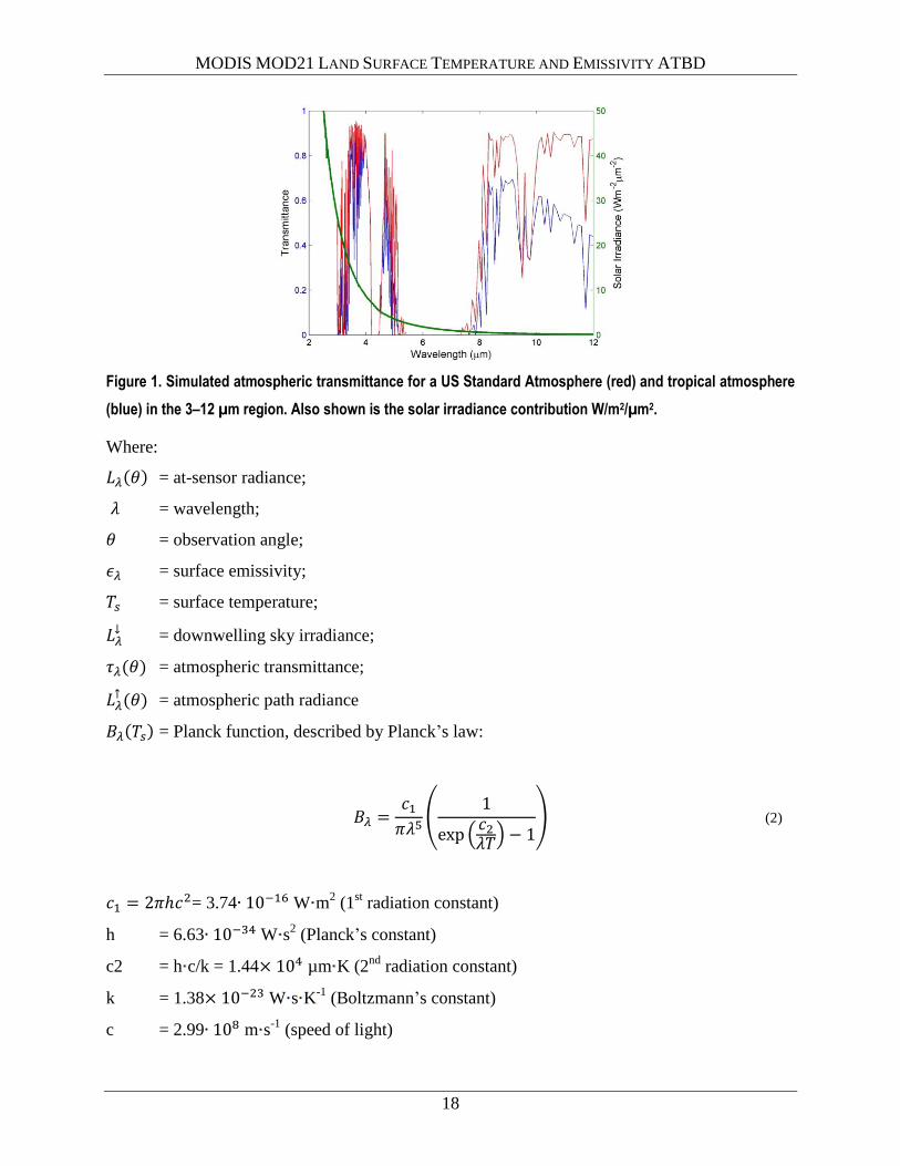
The at-sensor measured radiance in the TIR spectral region (7–14 µm) is a combination
of three primary terms: the Earth-emitted radiance, reflected downwelling sky irradiance, and
atmospheric path radiance. The Earth-emitted radiance is a function of temperature and
emissivity and gets attenuated by the atmosphere on its path to the satellite. The atmosphere also
emits radiation, some of which reaches the sensor directly as “path radiance,” while some gets
radiated to the surface (irradiance) and reflected back to the sensor, commonly known as the
reflected downwelling sky irradiance. Reflected solar radiation in the TIR region is negligible
(Figure 1) and a much smaller component than the surface-emitted radiance. One effect of the
sky irradiance is the reduction of the spectral contrast of the emitted radiance, due to Kirchhoff’s
law. Assuming the spectral variation in emissivity is small (Lambertian assumption), and using
Kirchhoff’s law to express the hemispherical-directional reflectance as directional emissivity
( the clear-sky at-sensor radiance can be written as three terms: the Earth-emitted
radiance described by Planck’s function and reduced by the emissivity factor, ; the reflected
downwelling irradiance; and the path radiance.
(1)
MODIS MOD21 LAND SURFACE TEMPERATURE AND EMISSIVITY ATBD
18
Figure 1. Simulated atmospheric transmittance for a US Standard Atmosphere (red) and tropical atmosphere
(blue) in the 3–12 µm region. Also shown is the solar irradiance contribution W/m2/µm2.
Where:
= at-sensor radiance;
= wavelength;
= observation angle;
= surface emissivity;
= surface temperature;
= downwelling sky irradiance;
= atmospheric transmittance;
= atmospheric path radiance
= Planck function, described by Planck’s law:
(2)
= 3.74 W m2 (1
st radiation constant)
h = 6.63 W s2 (Planck’s constant)
c2 = h c/k = 1.44 µm K (2nd
radiation constant)
k = 1.38 W s K-1
(Boltzmann’s constant)
c = 2.99 m s-1
(speed of light)
MODIS MOD21 LAND SURFACE TEMPERATURE AND EMISSIVITY ATBD
19
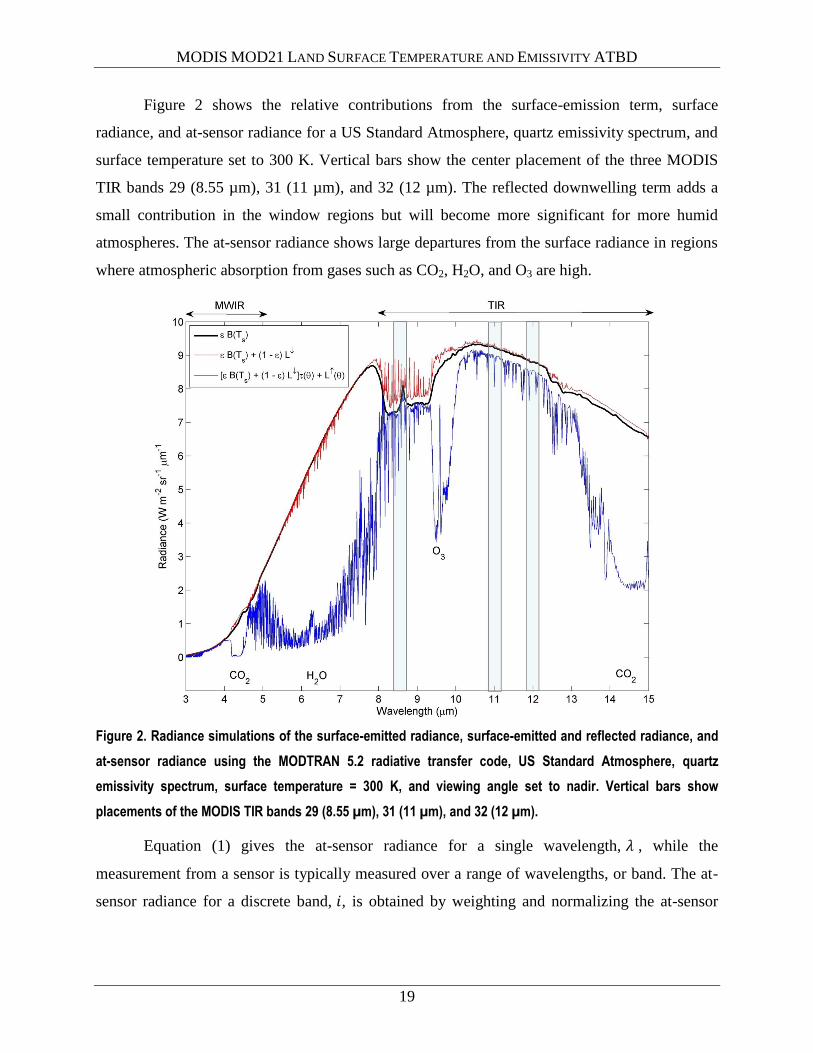
Figure 2 shows the relative contributions from the surface-emission term, surface
radiance, and at-sensor radiance for a US Standard Atmosphere, quartz emissivity spectrum, and
surface temperature set to 300 K. Vertical bars show the center placement of the three MODIS
TIR bands 29 (8.55 µm), 31 (11 µm), and 32 (12 µm). The reflected downwelling term adds a
small contribution in the window regions but will become more significant for more humid
atmospheres. The at-sensor radiance shows large departures from the surface radiance in regions
where atmospheric absorption from gases such as CO2, H2O, and O3 are high.
Figure 2. Radiance simulations of the surface-emitted radiance, surface-emitted and reflected radiance, and
at-sensor radiance using the MODTRAN 5.2 radiative transfer code, US Standard Atmosphere, quartz
emissivity spectrum, surface temperature = 300 K, and viewing angle set to nadir. Vertical bars show
placements of the MODIS TIR bands 29 (8.55 µm), 31 (11 µm), and 32 (12 µm).
Equation (1) gives the at-sensor radiance for a single wavelength, , while the
measurement from a sensor is typically measured over a range of wavelengths, or band. The at-
sensor radiance for a discrete band, , is obtained by weighting and normalizing the at-sensor
MODIS MOD21 LAND SURFACE TEMPERATURE AND EMISSIVITY ATBD
20
spectral radiance calculated by equation (1) with the sensor’s spectral response function for each
band, , as follows:
(3)
Using equations (1) and (2), the surface radiance for band can be written as a
combination of two terms: Earth-emitted radiance, and reflected downward irradiance from the
sky and surroundings:
(4)
The atmospheric parameters, , ,
, are estimated with a radiative transfer
model such as MODTRAN (Kneizys et al. 1996b) discussed in the next section, using input
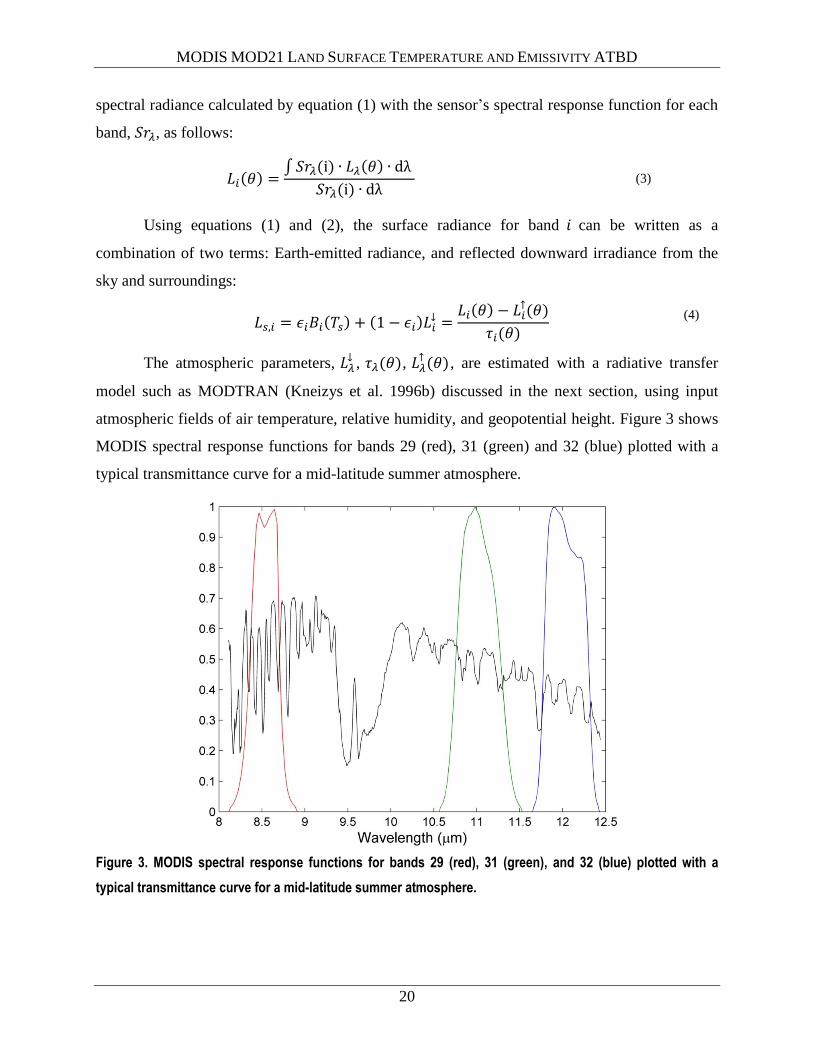
atmospheric fields of air temperature, relative humidity, and geopotential height. Figure 3 shows
MODIS spectral response functions for bands 29 (red), 31 (green) and 32 (blue) plotted with a
typical transmittance curve for a mid-latitude summer atmosphere.
Figure 3. MODIS spectral response functions for bands 29 (red), 31 (green), and 32 (blue) plotted with a
typical transmittance curve for a mid-latitude summer atmosphere.
MODIS MOD21 LAND SURFACE TEMPERATURE AND EMISSIVITY ATBD
21
4.2 Emissivity
The emissivity of an isothermal, homogeneous emitter is defined as the ratio of the actual
emitted radiance to the radiance emitted from a black body at the same thermodynamic
temperature (Norman and Becker 1995), = / . The emissivity is an intrinsic property of the
Earth’s surface and is an independent measurement of the surface temperature, which varies with
irradiance and local atmospheric conditions. The emissivity of most natural Earth surfaces for the
TIR wavelength ranges between 8 and 12 μm and, for a sensor with spatial scales <100 m, varies
from ~0.7 to close to 1.0. Narrowband emissivities less than 0.85 are typical for most desert and
semi-arid areas due to the strong quartz absorption feature (reststrahlen band) between the 8- and
9.5-μm range, whereas the emissivity of vegetation, water, and ice cover are generally greater
than 0.95 and spectrally flat in the 8–12-μm range.
4.3 Radiative Transfer Model
The current choice of radiative transfer model for atmospherically correcting MODIS
TIR data is the latest version of the Moderate Resolution Atmospheric Radiance and
Transmittance Model (MODTRAN) (Berk et al. 2005). MODTRAN has been sufficiently tested
and validated and meets the speed requirements necessary for high spatial resolution data
processing. The most recent MODTRAN 5.2 uses an improved molecular band model, termed
the Spectrally Enhanced Resolution MODTRAN (SERTRAN), which has a much finer
spectroscopy (0.1 cm-1
) than its predecessors (1–2 cm-1
), resulting in more accurate modeling of
band absorption features in the longwave TIR window regions (Berk et al. 2005). Furthermore,
validation with Line-by-Line models (LBL) has shown good accuracy.
Older versions of MODTRAN, such as version 3.5 and 4.0, have been used extensively in
the past few decades for processing multi-band and broadband TIR and short-wave/visible
imaging sensors such as ASTER data on NASA’s Terra satellite. Earlier predecessors, such as
MODTRAN 3.5, used a molecular band model with 2 cm-1
resolution and traced their heritage
back to previous versions of LOWTRAN (Berk 1989; Kneizys et al. 1996a). With the next
generation’s state-of-the-art, mid- and longwave IR hyperspectral sensors due for launch in the
next decade, there has been greater demand for higher resolution and quality radiative transfer
modeling. MODTRAN 5.2 has been developed to meet this demand by reformulating the
MODTRAN molecular band model line center and tail absorption algorithms. Further
MODIS MOD21 LAND SURFACE TEMPERATURE AND EMISSIVITY ATBD
22
improvements include the auxiliary species option, which simulates the effects of HITRAN-
specific trace molecular gases, and a new multiple scattering option, which improves the
accuracy of radiances in transparent window regions.
Wan and Li (2008) have compared MODTRAN 4 simulations with clear-sky radiances
from a well-calibrated, advanced Bomem TIR interferometer (MR100) and found accuracies to
within 0.1 K for brightness temperature-equivalent radiance values.
4.4 Atmospheric Profiles
The general methodology for atmospherically correcting the MODIS TIR data will be
based largely on the methods that were developed for the ASTER instrument (Palluconi et al.
1999). However, significant improvements will be made by taking advantage of newly
developed techniques and more advanced algorithms to improve accuracy. Currently two options
for atmospheric profile sources are available: 1) interpolation of data assimilated from Numerical
Weather Prediction (NWP) models, and 2) retrieved atmospheric geophysical profiles from
remote-sensing data. The NWP models use current weather conditions, observed from various
sources (e.g., radiosondes, surface observations, and weather satellites) as input to dynamic
mathematical models of the atmosphere to predict the weather. Data are typically output in 6-
hour increments, e.g., 00, 06, 12, and 18 UTC. Examples include: the Global Data Assimilation
System (GDAS) product provided by the National Centers for Environmental Prediction (NCEP)
(Kalnay et al. 1990); the Modern Era Retrospective-analysis for Research and Applications
(MERRA) product provided by the Goddard Earth Observing System Data Assimilation System
Version 5.2.0 (GEOS-5.2.0) (Bosilovich et al. 2008); and the European Center for Medium-
Range Weather Forecasting (ECMWF), which is supported by more than 32 European states.
Remote-sensing data, on the other hand, are available real-time, typically twice daily and for
clear-sky conditions. The principles of inverse theory are used to estimate a geophysical state
(e.g., atmospheric temperature) by measuring the spectral emission and absorption of some
known chemical species such as carbon dioxide in the thermal infrared region of the
electromagnetic spectrum (i.e., the observation). Examples of current remote-sensing data
include the Atmospheric Infrared Sounder (AIRS) (Susskind et al. 2003) and Moderate
Resolution Imaging Spectroradiometer (MODIS) (Justice and Townshend 2002), both on
NASA’s Aqua satellite launched in 2002.
MODIS MOD21 LAND SURFACE TEMPERATURE AND EMISSIVITY ATBD
23
The standard ASTER atmospheric correction technique, which is operated at the Land
Processes Distributed Active Archive Center (LP DAAC) at the EROS Center in Sioux Falls,
SD, uses input atmospheric profiles from the NCEP GDAS product at 1° spatial resolution and
6-hour intervals. An interpolation scheme in both space and time is required to characterize the
atmospheric conditions for an ASTER image on a pixel-by-pixel basis. This method could
potentially introduce large errors in estimates of air temperature and water vapor, especially in
humid regions where atmospheric water vapor can vary on smaller spatial scales than 1°. The
propagation of these atmospheric correction errors would result in band-dependent surface
radiance errors in both spectral shape and magnitude, which in turn would result in errors of
retrieved Level-2 products such as surface emissivity and temperature.
The plan for atmospherically correcting MODIS data for the MODTES algorithm will be to
use coincident profiles from the joint MODIS MOD07/MYD07 atmospheric product (Seemann
et al. 2003). The MOD07 product consists of profiles of temperature and moisture produced at
20 standard levels and total precipitable water vapor (TPW), total ozone, and skin temperature,
produced at 5 5 MODIS 1-km pixels. The latest MOD07 algorithm update (v5.2) includes a
new and improved surface emissivity training data set, with the result that RMSE differences in
TPW between MOD07 and a microwave radiometer (MWR) at the Atmospheric Radiation
Measurement (ARM) Southern Great Plains (SGP) site in Oklahoma were reduced from 2.9 mm
to 2.5 mm (Seemann et al. 2008). Other validation campaigns have included comparisons with
ECMWF and AIRS data, radiosonde observations (RAOBS), and MWR data at ARM SGP.
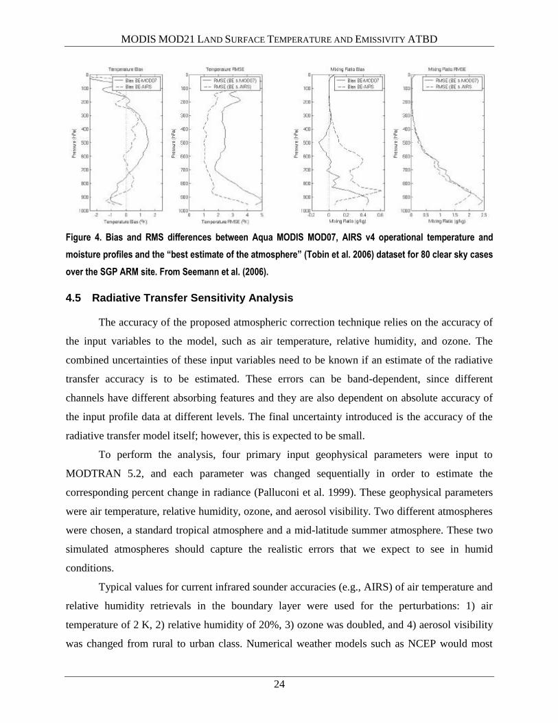
Figure 4 shows biases and RMS differences between Aqua MODIS MOD07 and the “best
estimate of the atmosphere” at the SGP ARMS site for air temperature (two left panels) and
water vapor mixing ratio (right two panels). Results show that MOD07 has a ~4 K RMSE at the
surface decreasing linearly to 2 K at 700 mb and then remaining at the 2–3 K until top of
atmosphere. For water vapor, the RMSE near the surface is ~2.5 g/kg and decreasing to
<0.5 g/kg above 600 mb.
MODIS MOD21 LAND SURFACE TEMPERATURE AND EMISSIVITY ATBD
24
Figure 4. Bias and RMS differences between Aqua MODIS MOD07, AIRS v4 operational temperature and
moisture profiles and the “best estimate of the atmosphere” (Tobin et al. 2006) dataset for 80 clear sky cases
over the SGP ARM site. From Seemann et al. (2006).
4.5 Radiative Transfer Sensitivity Analysis
The accuracy of the proposed atmospheric correction technique relies on the accuracy of
the input variables to the model, such as air temperature, relative humidity, and ozone. The
combined uncertainties of these input variables need to be known if an estimate of the radiative
transfer accuracy is to be estimated. These errors can be band-dependent, since different
channels have different absorbing features and they are also dependent on absolute accuracy of
the input profile data at different levels. The final uncertainty introduced is the accuracy of the
radiative transfer model itself; however, this is expected to be small.
To perform the analysis, four primary input geophysical parameters were input to
MODTRAN 5.2, and each parameter was changed sequentially in order to estimate the
corresponding percent change in radiance (Palluconi et al. 1999). These geophysical parameters
were air temperature, relative humidity, ozone, and aerosol visibility. Two different atmospheres
were chosen, a standard tropical atmosphere and a mid-latitude summer atmosphere. These two
simulated atmospheres should capture the realistic errors that we expect to see in humid
conditions.
Typical values for current infrared sounder accuracies (e.g., AIRS) of air temperature and
relative humidity retrievals in the boundary layer were used for the perturbations: 1) air
temperature of 2 K, 2) relative humidity of 20%, 3) ozone was doubled, and 4) aerosol visibility
was changed from rural to urban class. Numerical weather models such as NCEP would most

MODIS MOD21 LAND SURFACE TEMPERATURE AND EMISSIVITY ATBD
25
likely have larger uncertainties in the 1–2 K range for air temperature and 10–20% for relative
humidity (Kalnay et al. 1990).
Table 1 shows the results for three simulated MODIS bands 29, 31, and 32 expressed as
percent change in radiance (equivalent brightness temperature change in parentheses) for two
standard atmospheric regimes, tropical and mid-latitude summer. The results show that band 29
is in fact most sensitive to perturbations in air temperature, followed by band 31 and 32 for both
atmospheric profiles, with the mid-latitude profile having larger changes than tropical. For a 20%
change in humidity the reverse is true, band 32 having the largest change of nearly 3 K for a
tropical atmosphere, followed by band 31 and 29. This is because band 32 falls closest to strong
water lines above 12 µm, as shown in Figure 2. Doubling the ozone results in a much larger
sensitivity for band 5, since it is closest to the strong ozone absorption feature centered around
the 9.5-µm region as shown in Figure 2. Changing the aerosol visibility from rural to urban had a
small effect on each band but was largest for band 5. Generally, the radiance in the thermal
infrared region is insensitive to aerosols in the troposphere so, for the most part, a climatology-
based estimate of aerosols would be sufficient. However, when stratospheric aerosol amounts
increase substantially due to volcanic eruptions, for example, then aerosol amounts from future
NASA remote-sensing missions such as ACE and GEO-CAPE would need to be taken into
account.
Table 1. Percent changes in simulated at-sensor radiances for changes in input geophysical parameters for
MODIS bands 29, 31, and 32, with equivalent change in brightness temperature in parentheses.
Geophysical
Parameter
Change in
Parameter
% Change in Radiance
(Tropical Atmosphere)
% Change in Radiance
(Mid-lat Summer Atmosphere)
Band 29
(8.5 µm)
Band 31
(11 µm)
Band 32
(12 µm)
Band 29
(8.5 µm)
Band 31
(11 µm)
Band 32
(12 µm)
Air
Temperature
+2 K 2.8
(1.44 K)
1.97
(1.31 K)
1.62
(1.15 K)
3.27
(1.64 K)
2.50
(1.61 K)
2.13
(1.49 K)
Relative
Humidity
+20% 3.51
(1.76 K)
3.91
(2.54 K)
4.43
(3.09 K)
2.76
(1.35 K)
3.03
(1.93 K)
3.61
(2.48 K)
Ozone 0.69
(0.35 K)
0.00
(0 K)
0.02
(0.01 K)
0.69
(0.34 K)
0.00
(0 K)
0.02
(0.02 K)
Aerosol Urban/Rural 0.42
(0.21 K)
0.27
(0.17 K)
0.22
(0.16 K)
0.43
(0.21 K)
0.29
(0.19 K)
0.25
(0.17 K)
It should also be noted, as discussed in Palluconi et al. (1999), that in reality these types
of errors may have different signs, change with altitude, and/or have cross-cancelation between
MODIS MOD21 LAND SURFACE TEMPERATURE AND EMISSIVITY ATBD
26
the parameters. As a result, it is difficult to quantify the exact error budget for the radiative
transfer calculation; however, what we do know is that the challenging cases will involve warm
and humid atmospheres where distributions of atmospheric water vapor are the most uncertain.
5 Water Vapor Scaling Method
The accuracy of the TES algorithm is limited by uncertainties in the atmospheric
correction, which result in a larger apparent emissivity contrast. This intrinsic weakness of the
TES algorithm has been systemically analyzed by several authors (Coll et al. 2007; Gillespie et
al. 1998; Gustafson et al. 2006; Hulley and Hook 2009b; Li et al. 1999), and its effect is greatest
over graybody surfaces that have a true spectral contrast that approaches zero. In order to
minimize atmospheric correction errors, a Water Vapor Scaling (WVS) method has been
introduced to improve the accuracy of the water vapor atmospheric profiles on a band-by-band
basis for each observation using an Extended Multi-Channel/Water Vapor Dependent
(EMC/WVD) algorithm (Tonooka 2005), which is an extension of the Water Vapor Dependent
(WVD) algorithm (Francois and Ottle 1996). The EMC/WVD equation models the at-surface
brightness temperature, given the at-sensor brightness temperature, along with an estimate of the
total water vapor amount:
,
(5)
where:
Band number
Number of bands
Estimate of total precipitable water vapor (cm)
Regression coefficients for each band
Brightness temperature for band k (K)
Brightness surface temperature for band,
The coefficients of the EMC/WVD equation are determined using a global-based
simulation model with atmospheric data from the NCEP Climate Data Assimilation System
(CDAS) reanalysis project (Tonooka 2005).
MODIS MOD21 LAND SURFACE TEMPERATURE AND EMISSIVITY ATBD
27
The scaling factor, , used for improving a water profile, is based on the assumption that
the transmissivity, , can be express by the Pierluissi double exponential band model
formulation. The scaling factor is computed for each gray pixel on a scene using computed
from equation (4) and computed using two different values that are selected a priori:
(6)
where:
Band model parameter
Two appropriately chosen values
Transmittance calculated with water vapor profile scaled by
Path radiance calculated with water vapor profile scaled by
Typical values for are and . Tonooka (2005) found that the calculated
by equation (6) will not only reduce biases in the water vapor profile, but will also
simultaneously reduce errors in the air temperature profiles and/or elevation. An example of the
water vapor scaling factor, , is shown in Figure 6 for a MODIS observation on 29 August 2004.
5.1 Gray Pixel Computation
It is important to note that is only computed for graybody pixels (e.g., vegetation,
water, and some soils) with emissivities close to 1.0 and, as a result, an accurate gray-pixel
estimation method is required prior to processing. Vegetation indices such as the Normalized
Difference Vegetation Index (NDVI), land cover databases (e.g., MODIS MOD12), and thermal
log residuals (TLR) (Hook et al. 1992), are three different approaches that can be used in
combination to identify graybody pixels. In the MOD21 product all pixels with
photosynthetically active vegetation are first identified using the standard MODIS MOD13A2
(16-day) vegetation index product with an NDVI threshold (NDVI > 0.3). Water, ocean, and
snow/ice pixels are then classified using a land-water and snow-cover map generated from the
standard MODIS MOD10A2 product (8-day).
Using these gray pixels as a first-guess estimate, a TLR approach can be used to further
refine the gray-pixel map, but at present the uncertainties introduced by this approach are still too
high to use operationally. The TLR approach spectrally enhances images generated from multi-
MODIS MOD21 LAND SURFACE TEMPERATURE AND EMISSIVITY ATBD
28
spectral data and removes dependence on band-independent parameters such as surface
temperature. All gray pixels within a TLR image will have similar spectral features, and a
correlation coefficient approach is used to further refine the gray-pixel map based on the first-
guess gray pixels. For example, TLR pixels that have a correlation coefficient higher than 0.9
with the mean TLRs of the first guess gray pixels are further classified as graybodies. Figure 5
shows an example of the various stages of classifying graybodies for a MODIS scene cutout over
parts of Arizona and southeastern California (black = graybody, white = bare) on 29 August
2004. Using the NDVI and water mask all first-guess gray pixels are first classified (top right)
and then further refined with TLRs (bottom left) to produce the final graybody-pixel map.

MODIS MOD21 LAND SURFACE TEMPERATURE AND EMISSIVITY ATBD
29
Figure 5. Clockwise from top left: Google Earth visible image; first guess gray-pixel map; TLR refinement;
and final gray pixel map for a MODIS scene cutout over parts of Arizona and southeastern California
(black = graybody, white = bare) on 29 August 2004. See text for details.
5.2 Interpolation and Smoothing
Once is computed for all gray pixels, the values are horizontally interpolated to
adjacent bare pixels on the scene and smoothed before computing the improved atmospheric
parameters. An inverse distance-weighted interpolation method is typically used to fill in bare
MODIS MOD21 LAND SURFACE TEMPERATURE AND EMISSIVITY ATBD
30
pixel gaps. This is an interpolation method frequently used in numerical weather forecasting with
much success. The specific steps for interpolation of values are as follows:
1. First all bare pixels are set to 1; in addition, all values less than 0.2 and greater than 3 are
set to 1 for stability purposes and to eliminate possible cloud contamination.
2. Next, all cloudy pixels on the scene are set to not a number (NaN).
3. All bare pixels are then looped over, and optimum weights are found for all gray pixels
within a given effective radius of the bare pixel. The value for the pixel is then computed
using the weighted values surrounding the pixel and ignoring all NaN values as follows:
(7)
where is the number of gray pixels, and are the weight functions assigned to each gray
pixel value:
(8)
where is weighting factor, called the power parameter, typically set to 4. Higher values
give larger weights to the closest pixels. is the geometrical distance from the interpolation
pixel to the scattered points of interest within some effective radius (~50 km for MOD21 was
ideal):
(9)
where and are the coordinates of the interpolation point, and and are coordinates of
the scattered points.
If any bare pixels remain after the first pass, the bare pixels with a valid, calculated,
value are considered gray pixels, and the process is repeated until values for all bare pixels
have been computed.
This interpolation method should not introduce large error, since gray pixels are usually
widely available in any given MODIS scene and atmospheric profiles do not change significantly
at the medium-range scale (~50 km). Figure 6 shows an example of a image for band 29 after
interpolation and smoothing for the MODIS cutout shown in Figure 5.
MODIS MOD21 LAND SURFACE TEMPERATURE AND EMISSIVITY ATBD
31
Figure 6. MODIS MOD07 total column water vapor (left) and WVS factor, , (right) computed using equation
(5) for a MODIS scene cutout on 29 August 2004. The image has been interpolated and smoothed using the
techniques discussed in section 5.2.
5.3 Scaling Atmospheric Parameters
5.3.1 Transmittance and Path Radiance
Once the MODTRAN run has completed and the image has been interpolated and
smoothed, the atmospheric parameters transmittance and path radiance are modified as
follows:
(10)
(11)
Once the transmittance and path radiance have been adjusted using the scaling factor, the surface
radiance can be computed using equation (1).
5.3.2 Downward Sky Irradiance
In the WVS simulation model, the downward sky irradiance can be modeled using the
path radiance, transmittance, and view angle as parameters. To simulate the downward sky
irradiance in a MODTRAN run, the sensor target is placed a few meters above the surface, with
surface emission set to zero and view angle set at prescribed values, e.g., Gaussian angles
( = 0°, 11.6°, 26.1°, 40.3°, 53.7°, and 65°). In this way, the only radiance contribution is from
MODIS MOD21 LAND SURFACE TEMPERATURE AND EMISSIVITY ATBD
32
the reflected downwelling sky irradiance at a given view angle. The total sky irradiance
contribution is then calculated by summing up the contribution of all view angles over the entire
hemisphere:
(12)
where is the view angle and is the azimuth angle. However, to minimize computational time
in the MODTRAN runs, the downward sky irradiance can be modeled as a non-linear function of
path radiance at nadir view:
(13)
where , , and are regression coefficients (Table 2), and is computed by:
(14)
Tonooka (2005) found RMSEs of less than 0.07 W/m2/sr/µm for ASTER bands 10–14 when
using equation (13) as opposed to equation (12). Figure 7 shows an example of comparisons
between MODIS band 29 (8.55 µm) atmospheric transmittance (top), path radiance (middle), and
computed surface radiance (bottom), before and after applying the WVS scaling factor, , for the
MODIS cutout shown in Figure 5. A decrease in transmittance and corresponding increase in
path radiance values, after scaling over an area in the south of the image, show that the original
atmospheric water absorption was underestimated using input MODIS MOD07 atmospheric
profiles. The result is an increase in surface radiance over the bare regions of the Mojave Desert
in the south of the image due to an increase in reflected downward sky irradiance.
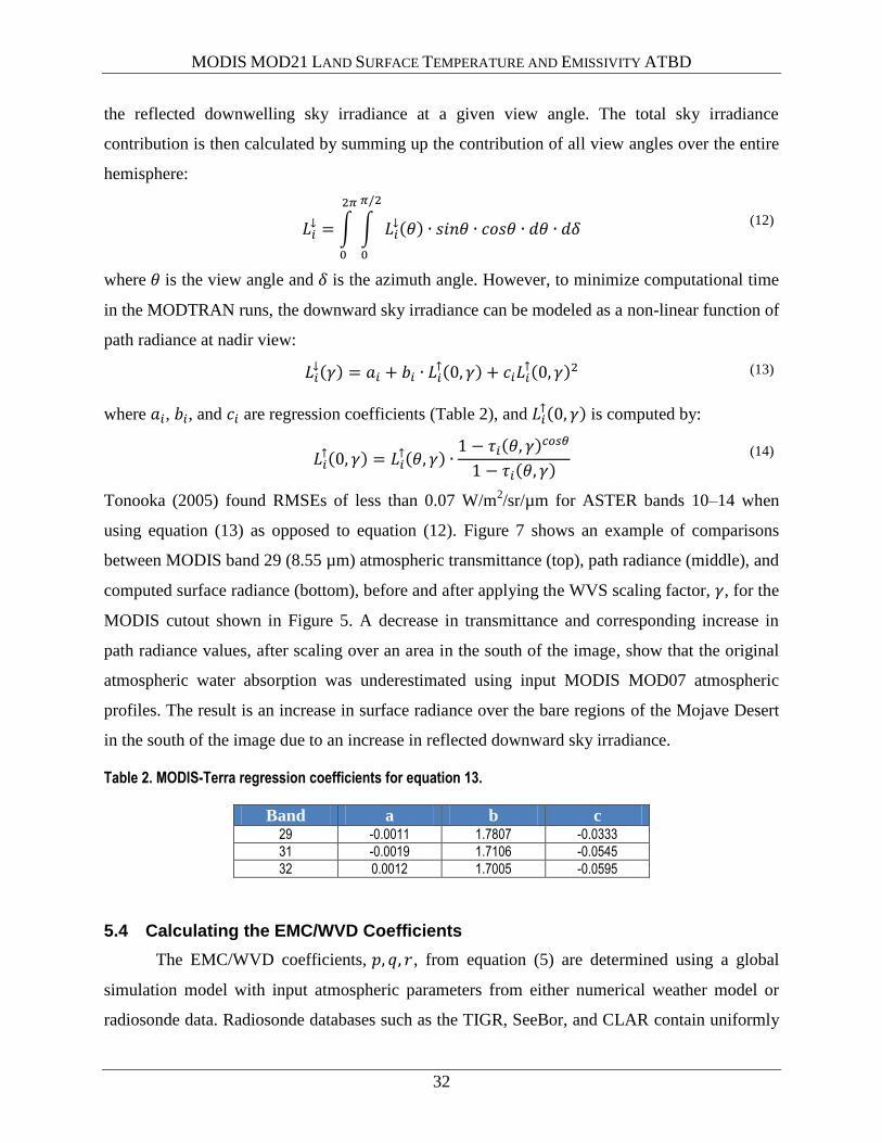
Table 2. MODIS-Terra regression coefficients for equation 13.
Band a b c 29 -0.0011 1.7807 -0.0333
31 -0.0019 1.7106 -0.0545
32 0.0012 1.7005 -0.0595
5.4 Calculating the EMC/WVD Coefficients
The EMC/WVD coefficients, , from equation (5) are determined using a global
simulation model with input atmospheric parameters from either numerical weather model or
radiosonde data. Radiosonde databases such as the TIGR, SeeBor, and CLAR contain uniformly

MODIS MOD21 LAND SURFACE TEMPERATURE AND EMISSIVITY ATBD
33
distributed global atmospheric soundings acquired both day and night in order to capture the full-
scale natural atmospheric variability.
Figure 7. Comparisons between the atmospheric transmittance (top), path radiance (W/m2/µm1) (middle),
and computed surface radiance (W/m2/µm1) (bottom), before and after applying the WVS scaling factor to
a MODIS scene cutout shown in Figure 5. Results are shown for MODIS band 29 (8.55 µm).

MODIS MOD21 LAND SURFACE TEMPERATURE AND EMISSIVITY ATBD
34
Geophysical profiles of air temperature, relative humidity, and geopotential height are
used in combination with surface temperature and emissivity to simulate at-sensor brightness
temperatures for the global set of profiles distributed uniformly over land. The air temperature
profiles are then shifted by 2, 0, and +2 K, while the humidity profiles are scaled by factors of
0.8, 1.0, and 1.2. These types of perturbations will help simulate a full range of atmospheric
conditions. Furthermore, the surface temperatures are modified by 5, 0, 5, and 10 K, and a set
of 10 surface emissivity spectra are provided. These spectra are typically from gray materials,
such as water, vegetation, snow, ice, and some types of soils, and tend to have values greater
than 0.95. This ensures that the simulation results are not affected by uncertainties in surface
emissivity, such as Lambertian effects. The at-sensor radiance is then computed using
MODTRAN for the full set of profiles and perturbations ( . The surface
elevation is taken from a global DEM (e.g., ASTER GDEM), and the view angle is assumed to
be nadir. Furthermore, a noise-equivalent differential temperature ( ) of 0.05 K appropriate
for MODIS thermal bands was applied using a normalized random number generator. Using the
simulated at-sensor , at-surface brightness temperatures, and an estimate of the total
precipitable water vapor, the coefficients in equation (5) were be found by using a linear least-
squares method. The coefficients are shown in Table 3 for MODIS bands 29, 31, and 32
including the RMSE (K). Table 4 shows the band model parameter coefficients used in equation
(6) to calculate the water vapor scaling factor.
Table 3. MODIS-Terra EMC/WVD coefficients used in equation (5).
Band pi,0 qi,0 ri,0 pi,1 qi,1 ri,1 pi,2 qi,2 ri,2 pi,3 qi,3 ri,3 RMSE
(K)
29 (i=1) -4.8338 20.0122 -0.005 -0.3757 -0.0768 0.0976 4.1226 1.1369 -0.1924 -2.7277 -1.1308 0.0952 1.395
31 (i=2) -3.6547 22.8787 -5.2738 -0.4274 -0.0491 0.1121 4.3162 1.0203 -0.2708 -2.8747 -1.0526 0.1778 0.682
32 (i=3) -3.7915 22.0713 -5.519 -0.4239 -0.0519 0.1174 4.2272 1.0663 -0.2914 -2.7881 -1.0932 0.1941 0.403
Table 4. MODIS-Terra band model parameters in equation (6).
Band Parameter
29 1.4293
31 1.8203
32 1.8344
MODIS MOD21 LAND SURFACE TEMPERATURE AND EMISSIVITY ATBD
35
6 Temperature and Emissivity Separation Approaches
The radiance in the TIR atmospheric window (8–13 µm) is dependent on the temperature
and emissivity of the surface being observed according to Planck’s law. Even if the atmospheric
properties (water vapor and air temperature) are well known and can be removed from equation
(1), the problem of retrieving surface temperature and emissivity from multispectral
measurements is still a non-deterministic process. This is because the total number of
measurements available (N bands) is always less than the number of variables to be solved for
(emissivity in N bands and one surface temperature). Therefore, no retrieval will ever do a
perfect job of separation, with the consequence that errors in temperature and emissivity may co-
vary. If the surface can be approximated as Lambertian (isotropic) and the emissivity is assigned
a priori from a land-cover classification, then the problem becomes deterministic with only the
surface temperature being the unknown variable. Examples of such cases would be over ocean,
ice, or densely vegetated scenes where the emissivity is known a priori and spectrally flat in all
bands. Another deterministic approach is the single-band inversion approach. If the atmospheric
parameters are known in equation (1), then the temperature can also be solved for using a single
band assuming the emissivity is known, usually in the clearest region of the window (~11 µm).
Deterministic approaches are usually employed with sensors that have one or two bands in the
TIR region using an SW approach, while non-deterministic approaches are applied to
multispectral sensors with three or more bands in the TIR so that spectral variations in the
retrieved emissivity can be related to surface composition and cover, in addition to retrieving the
surface temperature. For the MODIS MOD21 product, a non-deterministic approach will be used
in order to retrieve spectral emissivity in bands 29, 31, and 32, in addition to the surface
temperature.
6.1 Deterministic Approaches
6.1.1 SW Algorithms
The most common deterministic approach can be employed without having to explicitly
solve the radiative transfer equation. Two or more bands are employed in the window region
(typically 10.5–12 µm), and atmospheric effects are compensated for by the differential
absorption characteristics from the two bands. This approach is used with much success over
oceans to compute the SST (Brown and Minnett 1999), as the emissivity of water is well known
MODIS MOD21 LAND SURFACE TEMPERATURE AND EMISSIVITY ATBD
36
(Masuda et al. 1988). Variations of this method over land include the SW approach (Coll and
Caselles 1997; Prata 1994; Price 1984; Wan and Dozier 1996; Yu et al. 2008), the multichannel
algorithm (Deschamps and Phulpin 1980), and the dual-angle algorithm (Barton et al. 1989).
Over land, the assumption is that emissivities in the SW bands being used are stable and well
known and can be assigned using a land-cover classification map (Snyder et al. 1998). However,
this assumption introduces large errors over barren surfaces where much larger variations in
emissivity are found due to the presence of large amounts of exposed rock or soil, often with
abundant silicates (Hulley and Hook 2009a). Land cover classification maps typically use
Visible Near-Infrared (VNIR) data for assignment of various classes. This method may work for
most vegetation types and over water surfaces but, because VNIR reflectances correspond
predominately to Fe oxides and OH and not to the Si-O bond over barren areas, there is little or
no correlation with silicate mineralogy features in thermal infrared data. This is why, in most
classification maps, only one bare land class is specified (barren).
The primary LST product for MODIS (MOD11) currently uses a generalized SW
approach (Wan and Dozier 1996), where coefficients are stratified according to view angle, total
column water (TCW), and surface air temperature. Emissivities are assigned a priori based on
land cover classification maps. The MOD21 LST&E product will not be based on an SW
algorithm as in MOD11, but will use a non-deterministic multi-spectral approach for the
following reasons:
1. An SW method based on classification is not able to retrieve spectral emissivities of geologic
surfaces for compositional analysis.
2. The emissivity of the land surface is in general heterogeneous and is dependent on many
factors including surface soil moisture, vegetation cover changes, and surface compositional
changes, which are not characterized by land classification maps.
3. SW algorithms are inherently very sensitive to measurement noise between bands.
4. Classification leads to sharp discontinuities and contours in the data between different class
types, while a physical-based multispectral retrieval will produce seamless emissivity
images.
5. Temperature inaccuracies are difficult to quantify over geologic surfaces where constant
emissivities are assigned.
MODIS MOD21 LAND SURFACE TEMPERATURE AND EMISSIVITY ATBD
37
6.1.2 Single-Band Inversion
If the atmosphere is known, along with an estimate of the emissivity, then equation (1)
can be inverted to retrieve the surface temperature using one band. Theoretically, any band used
should retrieve the same temperature, but uncertainties in the atmospheric correction will result
in subtle differences as different bands have stronger atmospheric absorption features than others
that may be imperfectly corrected for atmospheric absorption. For example, a band near 8 µm
will have larger dependence on water vapor, while the 9–10-µm region will be more susceptible
to ozone absorption. Jimenez-Munoz and Sobrino (2010) applied this method to ASTER data by
using atmospheric functions (AFs) to account for atmospheric effects. The AFs can be computed
by the radiative transfer equation or empirically given the total water vapor content. The clearest
ASTER band (13 or 14) was used to retrieve the temperature, with the emissivity determined
using an NDVI fractional vegetation cover approach. A similar procedure has been proposed to
retrieve temperatures from the Landsat TIR band 6 on ETM+ and TM sensors (Li et al. 2004).
The single-band inversion method has not been proposed for MODIS data for the following
reasons:
1. Inability to retrieve spectral emissivity of geologic surfaces for compositional analysis. This
will not be possible with the single-band approach, which assigns emissivity based on land
cover type and vegetation fraction.
2. Estimating emissivity from an NDVI-derived vegetation cover fraction over arid and semi-
arid regions will introduce errors in the LST because NDVI is responsive only to
chlorophyll-active vegetation, and does not correlate well with senescent vegetation (e.g.,
shrublands).
3. Only one-band emissivity is solved for the single-band inversion approach. The MODIS
MOD21 product will be based on a multispectral retrieval approach.
6.1.3 Non-deterministic Approaches
In non-deterministic approaches, the temperature and spectral emissivity are solved using
an additional constraint or extra degree of freedom that is independent of the data source. These
types of solutions are also rarely perfect because the additional constraint will always introduce
an additional level of uncertainty; however, they work well over all surfaces (including arid and
semi-arid) and can automatically account for land surface changes, such as those due to wildfires
MODIS MOD21 LAND SURFACE TEMPERATURE AND EMISSIVITY ATBD
38
or surface soil moisture. First, we introduce two well-known approaches, the day/night and TISI
algorithms, followed by an examination of the algorithms and methods that led up to
establishment of the TES algorithm, which will be used in the MOD21 LST&E product.
6.1.3.1 Day/Night Algorithm
The constraint in the day/night algorithm capitalizes on the fact that the emissivity is an
intrinsic property of the surface and should not change from day- to nighttime observations. The
day/night algorithm is currently used to retrieve temperature/emissivity from MODIS data in the
MOD11B1 product (Wan and Li 1997). The method relies on two measurements (day and night),
and the theory is as follows: Two observations in N bands produce 2N observations, with the
unknown variables being N-band emissivities, a day- and nighttime surface temperature, four
atmospheric variables (day and night air temperature and water vapor), and an anisotropic factor,
giving N + 7 variables. In order to make the problem deterministic, the following conditions
must be met: 2N ≥ N+7, or N ≥ 7. For the MODIS algorithm, this can be satisfied by using bands
20, 22, 23, 29, and 31–33. Although this method is theoretically sound, the retrieval is
complicated by the fact that two clear, independent observations are needed (preferably close in
time) and the pixels from day and night should be perfectly co-registered. Errors may be
introduced when the emissivity changes from day to night observation (e.g., due to condensation
or dew), and from undetected nighttime cloud. In addition, the method relies on very precise co-
registration between the day- and nighttime pixel.
6.1.3.2 Temperature Emissivity Separation Approaches
During research activities leading up to the ASTER mission, the ASTER TEWG was
established in order to examine the performance of existing non-deterministic algorithms and
select one that would be suitable for retrieving the most accurate temperature and/or emissivity
over the entire range of terrestrial surfaces. This led to the development of the TES algorithm,
which ended up being a hybrid algorithm that capitalized on the strengths of previous algorithms.
In Gillespie et al. (1999), ten inversion algorithms were outlined and tested, leading up to
development of TES. For all ten algorithms, an independent atmospheric correction was
necessary. The ten algorithms were as follows: 1) Alpha-derived emissivity (ADE) method, 2)
Classification method, 3) Day-Night measurement, 4) Emissivity bounds method, 5) Graybody
MODIS MOD21 LAND SURFACE TEMPERATURE AND EMISSIVITY ATBD
39
emissivity method, 6) Mean Min-Max Difference (MMD) method, 7) Model emissivity method,
8) Normalized emissivity method (NEM), 9) Ratio Algorithm, and 10) SW algorithm.
In this document, we will briefly discuss a few of the algorithms but will not expand
upon any of them in great detail. The Day-Night measurement (3), Classification (2), and SW
(10) algorithms have already been discussed in section 4.2.1. A detailed description of all ten
algorithms is available in Gillespie et al. (1999). The various constraints proposed in these
algorithms can: determine spectral shape but not temperature, use multiple observations (day and
night), assume a value for emissivity and calculate temperature, assume a spectral shape, or
assume a relationship between spectral shape and minimum emissivity.
The NEM removes the downwelling sky irradiance component by assuming an of
0.99. Temperature is then estimated by inverting the Planck function and a new emissivity found.
This process is repeated until successive changes in the estimated surface radiances are small.
This method in itself was not found to be suitable for ASTER because temperature inaccuracies
tended to be high (>3 K) and the emissivities had incorrect spectral shapes. Other approaches
have used a model to estimate emissivity at one wavelength (Lyon 1965) or required that the
emissivity be the same at two wavelengths (Barducci and Pippi 1996). This introduces problems
for multispectral data with more than five bands, e.g., ASTER.
The ADE method (Hook et al. 1992; Kealy et al. 1990; Kealy and Hook 1993) is based
on the alpha residual method that preserves emissivity spectral shape but not amplitude or
temperature. The introduced constraint uses an empirical relationship between spectral contrast
and average emissivity to restore the amplitude of the alpha-residual spectrum and to compute
temperature. The average emissivity was used in the relationship to minimize band-to-band
calibration errors. The TEWG used this key feature of the ADE method in TES, although the
minimum emissivity, rather than the average emissivity, was used in the empirical relationship
(Matsunaga 1994). The ADE itself was not fully employed for two primary reasons as discussed
in Gillespie et al. (1999): 1) ADE uses Wien’s approximation, exp(x) 1 = exp(x), which
introduces a noticeable “tilt” in the residual spectra that gets transferred to the final emissivity
spectra; and 2) This issue was easily fixed in the hybrid version of TES.
Lastly, the temperature-independent spectral indices (TISI) approach (Becker and Li
1990) computes relative emissivities from power-scaled brightness temperatures. TISI, however,
is band-dependent and only recovers spectral shape; furthermore, the values are non-unique. To
MODIS MOD21 LAND SURFACE TEMPERATURE AND EMISSIVITY ATBD
40
retrieve actual emissivities, additional information or assumptions are needed. Other algorithms,
which only retrieve spectral shape, are the thermal log and alpha residual approach (Hook et al.
1992) and spectral emissivity ratios (Watson 1992; Watson et al. 1990). Neither of these was
considered because they do not recover temperature or actual emissivity values.
6.2 TES Algorithm
The final TES algorithm proposed by the ASTER TEWG combined some core features
from previous algorithms and, at the same time, improved on them. TES combines the NEM, the
ratio, and the MMD algorithm to retrieve temperature and a full emissivity spectrum. The NEM
algorithm is used to estimate temperature and iteratively remove the sky irradiance, from which
an emissivity spectrum is calculated, and then ratioed to their mean value in the ratio algorithm.
At this point, only the shape of the emissivity spectrum is preserved, but not the amplitude. In
order to compute an accurate temperature, the correct amplitude is then found by relating the
minimum emissivity to the spectral contrast (MMD). Once the correct emissivities are found, a
final temperature can be calculated with the maximum emissivity value. Additional
improvements involve a refinement of in the NEM module and refining the correction for
sky irradiance using the -MMD final emissivity and temperature values. Finally, a quality
assurance (QA) data image is produced that partly depends on outputs from TES such as
convergence, final , atmospheric humidity, and proximity to clouds. More detailed
discussion of QA is included later in this document.
Numerical modeling studies performed by the ASTER TEWG showed that TES can
recover temperatures to within 1.5 K and emissivities to within 0.015 over most scenes,
assuming well-calibrated, accurate radiometric measurements (Gillespie et al. 1998).
6.2.1 TES Data Inputs
Inputs to the TES algorithm are the surface radiance, , given by equation (4) (at-
sensor radiance corrected for transmittance and path radiance), and downwelling sky irradiance
term, , which is computed from the atmospheric correction algorithm using a radiative transfer
model such as MODTRAN. Both the surface radiance and sky irradiance will be output as a
separate product. The surface radiance is primarily used as a diagnostic tool for monitoring
changes in Earth’s surface composition. Before the surface radiance is estimated using equation
(4), the accuracy of the atmospheric parameters, , ,
, is improved upon using a
MODIS MOD21 LAND SURFACE TEMPERATURE AND EMISSIVITY ATBD
41
WVS method (Tonooka 2005) on a band-by-band basis for each observation using an extended
multi-channel/water vapor dependent (EMC/WVD) algorithm.
6.2.2 TES Limitations
As with any retrieval algorithm, limitations exist that depend on measurement accuracy,
model errors, and incomplete characterization of atmospheric effects. Currently, the largest
source of uncertainty for ASTER data is the residual effect of incomplete atmospheric correction.
Measurement accuracy and precision contribute to a lesser degree. This problem is compounded
for graybodies, which have low spectral contrast and are therefore more prone to errors in
“apparent” MMD, which is overestimated due to residual sensor noise and incomplete
atmospheric correction. A threshold classifier was introduced by the TEWG to partly solve this
problem over graybody surfaces. Instead of using the calibration curve to estimate from
MMD, a value of = 0.983 was automatically assigned when the spectral contrast or MMD in
emissivity was smaller than 0.03 for graybody surfaces (e.g., water, vegetation). However, this
caused artificial step discontinuities in emissivity between vegetated and arid areas.
At the request of users, two parameter changes were made to the ASTER TES algorithm
on 1 August 2007, first described in Gustafson et al. (2006). Firstly, the threshold classifier was
removed as it caused contours and artificial boundaries in the images, which users could not
tolerate in their analyses. The consequence of removing the threshold classifier was a smoother
appearance for all images but at the cost of TES underestimating the emissivity of graybody
scenes, such as water by up to 3% and vegetation by up to 2% (Hulley et al. 2008). The second
parameter change removed the iterative correction for reflected downwelling radiation, which
also frequently failed due to inaccurate atmospheric corrections (Gustafson et al. 2006). Using
only the first iteration resulted in improved spectral shape and performance of TES.
Figure 8 shows the distribution of LST uncertainties for the MODIS and ASTER TES
algorithm with respect to TCW and simulated LST for TES+atm (atmospheric uncertainty) and
TES+atm+wvs (atmospheric uncertainty with WVS) simulation cases. In general the TES+atm
uncertainties increase with TCW and simulated LST for both types of surfaces and range from
4–6 K for TCW values greater than 4 cm and LSTs greater than 300 K. The TES+atm+wvs
results show that applying the WVS method reduces the LST uncertainty at higher TCW
contents by more than a factor of two, with uncertainties not exceeding 2 K for either type of
surface type or sensor.
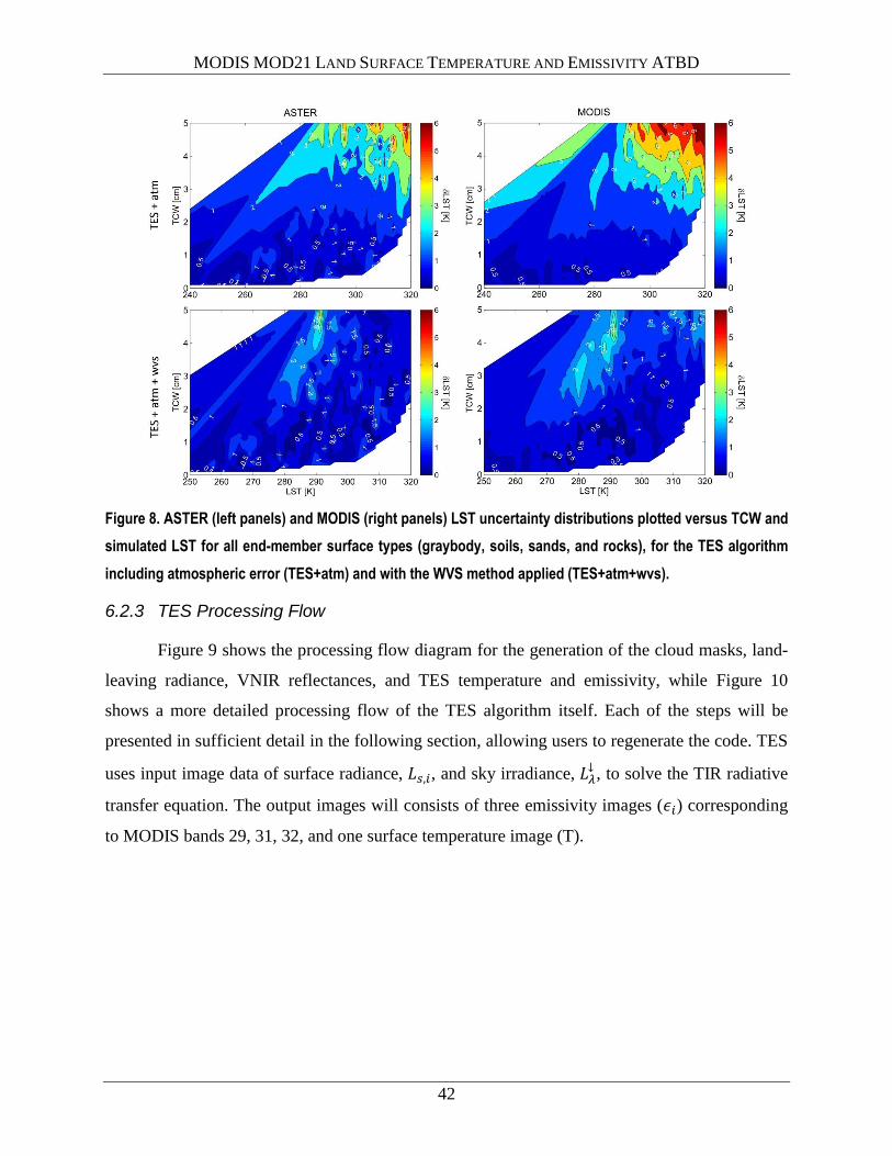
MODIS MOD21 LAND SURFACE TEMPERATURE AND EMISSIVITY ATBD
42
Figure 8. ASTER (left panels) and MODIS (right panels) LST uncertainty distributions plotted versus TCW and
simulated LST for all end-member surface types (graybody, soils, sands, and rocks), for the TES algorithm
including atmospheric error (TES+atm) and with the WVS method applied (TES+atm+wvs).
6.2.3 TES Processing Flow
Figure 9 shows the processing flow diagram for the generation of the cloud masks, land-
leaving radiance, VNIR reflectances, and TES temperature and emissivity, while Figure 10
shows a more detailed processing flow of the TES algorithm itself. Each of the steps will be
presented in sufficient detail in the following section, allowing users to regenerate the code. TES
uses input image data of surface radiance, , and sky irradiance, , to solve the TIR radiative
transfer equation. The output images will consists of three emissivity images ( ) corresponding
to MODIS bands 29, 31, 32, and one surface temperature image (T).
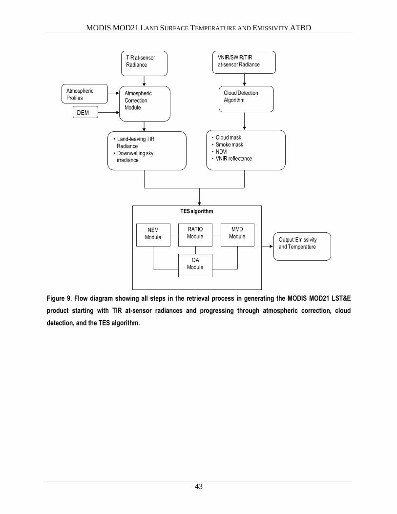
MODIS MOD21 LAND SURFACE TEMPERATURE AND EMISSIVITY ATBD
43
Figure 9. Flow diagram showing all steps in the retrieval process in generating the MODIS MOD21 LST&E
product starting with TIR at-sensor radiances and progressing through atmospheric correction, cloud
detection, and the TES algorithm.
Cloud Detection
Algorithm
• Cloud mask
• Smoke mask
• NDVI• VNIR reflectance
Atmospheric
Correction
Module
• Land-leaving TIR
Radiance
• Downwelling sky irradiance
Atmospheric
Profiles
TES algorithm
NEM
Module
RATIO
Module
MMD
Module
QA
Module
DEM
Output: Emissivity
and Temperature
TIR at-sensor
Radiance
VNIR/SWIR/TIR
at-sensor Radiance
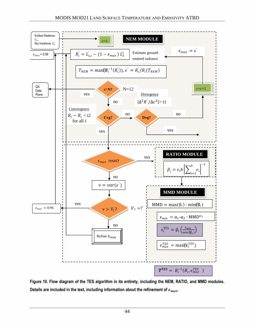
MODIS MOD21 LAND SURFACE TEMPERATURE AND EMISSIVITY ATBD
44
Figure 10. Flow diagram of the TES algorithm in its entirety, including the NEM, RATIO, and MMD modules.
Details are included in the text, including information about the refinement of .
Surface Radiance:
,
Sky Irradiance:
′ = ,
′ (1 𝑚 ) Estimate ground-
emitted radiance
𝑀 = max( 1
′ ), ′ = ′/ ( 𝑀)
c=c+1 c>N?
yes
no
Cvg?
′ < t2
for all
yes
Dvg? no
𝑚 = ′
NEM MODULE
no
yes
2 ′/ 2 > t1
Divergence
Convergence
N=12
𝜈 = 𝑣 ( ′)
c=1
ν > V1?
' > ?
𝑉1 =? yes
𝑚 reset?
no
Refine ϵmax
no
yes
RATIO MODULE
𝛽 =
=1
1
MMD MODULE
ϵmin = α1-α2 MMDα3
MMD = max βi - min(βi)
ϵiTES = βi
ϵmin
min (β i )
𝑻𝑻𝑬𝑺 = 1
′ , 𝑚
𝑚 = max(
)
𝑚 = 0.99
𝑚 = 0.96
QA Data Plane
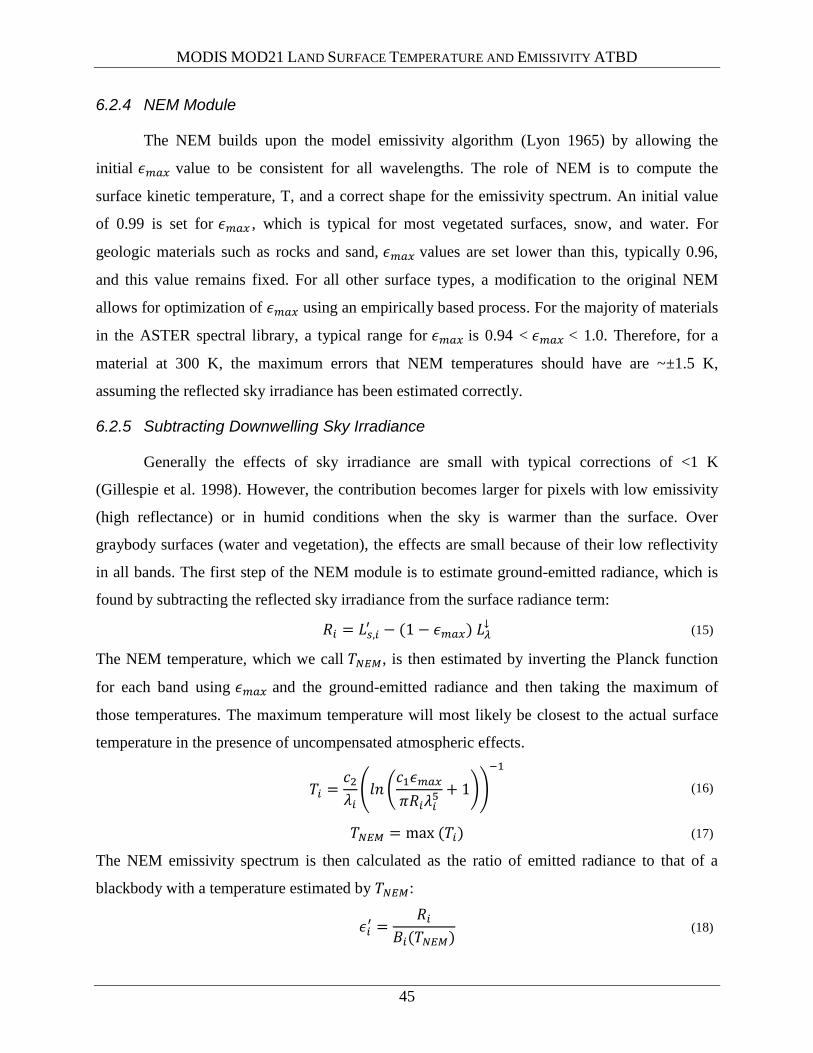
MODIS MOD21 LAND SURFACE TEMPERATURE AND EMISSIVITY ATBD
45
6.2.4 NEM Module
The NEM builds upon the model emissivity algorithm (Lyon 1965) by allowing the
initial value to be consistent for all wavelengths. The role of NEM is to compute the
surface kinetic temperature, T, and a correct shape for the emissivity spectrum. An initial value
of 0.99 is set for , which is typical for most vegetated surfaces, snow, and water. For
geologic materials such as rocks and sand, values are set lower than this, typically 0.96,
and this value remains fixed. For all other surface types, a modification to the original NEM
allows for optimization of using an empirically based process. For the majority of materials
in the ASTER spectral library, a typical range for is 0.94 < < 1.0. Therefore, for a
material at 300 K, the maximum errors that NEM temperatures should have are ~±1.5 K,
assuming the reflected sky irradiance has been estimated correctly.
6.2.5 Subtracting Downwelling Sky Irradiance
Generally the effects of sky irradiance are small with typical corrections of <1 K
(Gillespie et al. 1998). However, the contribution becomes larger for pixels with low emissivity
(high reflectance) or in humid conditions when the sky is warmer than the surface. Over
graybody surfaces (water and vegetation), the effects are small because of their low reflectivity
in all bands. The first step of the NEM module is to estimate ground-emitted radiance, which is
found by subtracting the reflected sky irradiance from the surface radiance term:
(15)
The NEM temperature, which we call , is then estimated by inverting the Planck function
for each band using and the ground-emitted radiance and then taking the maximum of
those temperatures. The maximum temperature will most likely be closest to the actual surface
temperature in the presence of uncompensated atmospheric effects.
(16)
(17)
The NEM emissivity spectrum is then calculated as the ratio of emitted radiance to that of a
blackbody with a temperature estimated by :
(18)
MODIS MOD21 LAND SURFACE TEMPERATURE AND EMISSIVITY ATBD
46
The new emissivity spectrum is then used to re-calculate
, and the process
is repeated until convergence, which is determined if the change in between steps is less than
a set threshold, , which is set as the radiance equivalent to NEΔT of the sensor. The process is
stopped if the number of iterations exceeds a limit N, set to 12. Execution of the NEM module is
also aborted if the slope of versus iteration, , increases such that > , where is
also set to radiance equivalent of NEΔT for the sensor (0.05 K for MODIS). In this case,
correction is not possible, TES is aborted, and NEM values of and are reported in the
QA data plane, along with an error flag. TES is also aborted and an error flag recorded if, for any
iteration, the values of fall out of reasonable limits, set to . See Figure 10 for a
detailed description of these steps.
6.2.6 Refinement of
Most pixels at MODIS resolution (1 km) will contain a mixed cover type consisting of
vegetation and soil, rock and water. The effective maximum emissivity for such pixels will
therefore vary across the scene and depend on the fractional contribution of each cover type. For
these cases, the initial = 0.99 may be set to high and refinement of is necessary to
improve accuracy of . The optimal value for minimizes the variance, 𝜈, of the NEM
calculated emissivities, . The optimization of is only useful for pixels with low emissivity
contrast (near graybody surfaces) and therefore is only executed if the variance for = 0.99 is
less than an empirically determined threshold (e.g., 𝑉 for ASTER ) (Gillespie et
al. 1998). If the variance is greater than 𝑉 , then the pixel is assumed to predominately consist of
either rock or soil. For this case, is reset to 0.96, which is a good first guess for most rocks
and soils in the ASTER spectral library, which typically fall between the 0.94 and 0.99 range.
For MODIS the values is set to 0.97, a typical value for bare surfaces in the 12 µm range. If
the first condition is met, and the pixel is a near-graybody, then values for of 0.92, 0.95,
0.97, and 0.99 are used to compute the variance for each corresponding NEM emissivity
spectrum. A plot of variance 𝜈 versus each value results in an upward-facing parabola with
the optimal value determined by the minimum of the parabola curve in the range
. This minimum is set to a new value, and the NEM module is executed again to
compute a new . Further tests are used to see if a reliable solution can be found for the
refined . If the parabola is too flat, or too steep, then refinement is aborted and the original
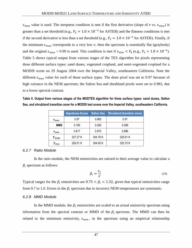
MODIS MOD21 LAND SURFACE TEMPERATURE AND EMISSIVITY ATBD
47
value is used. The steepness condition is met if the first derivative (slope of 𝜈 vs. ) is
greater than a set threshold (e.g., 𝑉 for ASTER) and the flatness conditions is met
if the second derivative is less than a set threshold (e.g., 𝑉 for ASTER). Finally, if
the minimum corresponds to a very low 𝜈, then the spectrum is essentially flat (graybody)
and the original = 0.99 is used. This condition is met if 𝜈 𝑉 (e.g., 𝑉 ).
Table 5 shows typical output from various stages of the TES algorithm for pixels representing
three different surface types: sand dunes, vegetated cropland, and semi-vegetated cropland for a
MODIS scene on 29 August 2004 over the Imperial Valley, southeastern California. Note the
different value for each of these surface types. The dune pixel was set to 0.97 because of
high variance in the NEM spectrum; the Salton Sea and shrubland pixels were set to 0.983, due
to a lower spectral contrast.
Table 5. Output from various stages of the MODTES algorithm for three surface types: sand dunes, Salton
Sea, and shrubland transition zone for a MODIS test scene over the Imperial Valley, southeastern California.
Algodones Dunes Salton Sea Shrubland (transition zone)
0.97 0.983 0.97
MMD 0.166 0.006 0.088
0.817 0.975 0.886
𝑻 𝑬 327.27 K 304.76 K 325.61 K
𝑻𝑻𝑬𝑺 326.51 K 304.95 K 325.75 K
6.2.7 Ratio Module
In the ratio module, the NEM emissivities are ratioed to their average value to calculate a
𝛽 spectrum as follows:
𝛽
(19)
Typical ranges for the 𝛽 emissivities are 𝛽 , given that typical emissivities range
from 0.7 to 1.0. Errors in the 𝛽 spectrum due to incorrect NEM temperatures are systematic.
6.2.8 MMD Module
In the MMD module, the 𝛽 emissivities are scaled to an actual emissivity spectrum using
information from the spectral contrast or MMD of the 𝛽 spectrum. The MMD can then be
related to the minimum emissivity, , in the spectrum using an empirical relationship
MODIS MOD21 LAND SURFACE TEMPERATURE AND EMISSIVITY ATBD
48
determined from lab measurements of a variety of different spectra, including rocks, soils,
vegetation, water, and snow/ice. From , the actual emissivity spectrum can be found by re-
scaling the 𝛽 spectrum. First, the MMD of the 𝛽 spectrum is found by:
𝑀𝑀 𝛽 𝛽 (20)
Then MMD can be related to using a power-law relationship:
𝑀𝑀 , (21)
where are coefficients that are obtained by regression using lab measurements. For the three
MODIS TIR bands between 8 and 12 µm (shown in Figure 2), the values for the coefficients
were calculated as = 0.985, , and . The TES emissivities are then
calculated by re-scaling the 𝛽 emissivities:
𝛽
𝛽
(22)
An example MODTES emissivity output image for band 29 (8.55 µm) is shown in Figure
11 for an MODIS cutout on 29 August 2004 over the Imperial Valley, southeastern California.
Bare areas, such as the Algodones Dunes running diagonally across the southeast corner,
generally have emissivity <0.85, while graybody surfaces such as the Imperial Valley croplands
and Salton Sea in the southwest corner of the image have higher emissivities, >0.95. Figure 12
shows the differences in emissivity spectra between the NEM and TES output for pixels over
three different surface types (sand dunes, Salton Sea water, and mixed shrubland) for the
Imperial Valley cutout. Note that, although both NEM and TES have similar spectral shape, the
emissivities of NEM are generally higher than TES because of the initial estimate of in the
NEM module. The Algodones Dunes spectrum has high spectral contrast, which is typical for a
quartz spectrum that has the characteristic quartz doublet in the 8–10-µm region, while the
emissivity of water is usually spectrally flat, and high.
For pixels with low spectral contrast (e.g., graybody surfaces), the accuracy of MMD
calculated from TES is compromised and approaches a value that depends on measurement error
and residual errors from incomplete atmospheric correction. For ASTER, which has a NEΔT of
0.3 K at 300 K, measurement error contributes to the apparent contrast, and a method was
explored to correct the apparent MMD using Monte Carlo simulations. For MODIS (NEΔT of
0.05 K), we expect measurement errors to be minimal and atmospheric effects to be the largest
contribution to MMD errors. A further problem for graybody surfaces is a loss of precision for
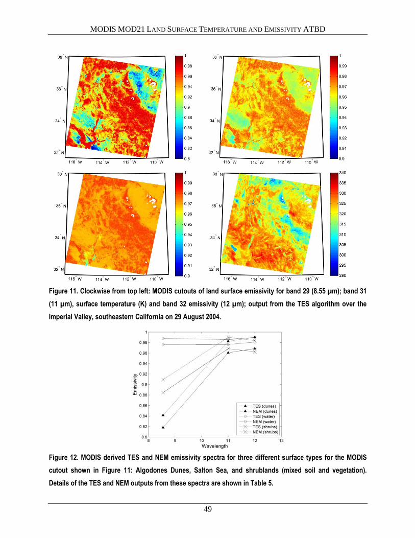
MODIS MOD21 LAND SURFACE TEMPERATURE AND EMISSIVITY ATBD
49
Figure 11. Clockwise from top left: MODIS cutouts of land surface emissivity for band 29 (8.55 µm); band 31
(11 µm), surface temperature (K) and band 32 emissivity (12 µm); output from the TES algorithm over the
Imperial Valley, southeastern California on 29 August 2004.
Figure 12. MODIS derived TES and NEM emissivity spectra for three different surface types for the MODIS
cutout shown in Figure 11: Algodones Dunes, Salton Sea, and shrublands (mixed soil and vegetation).
Details of the TES and NEM outputs from these spectra are shown in Table 5.
MODIS MOD21 LAND SURFACE TEMPERATURE AND EMISSIVITY ATBD
50
low MMD values. This is due to the shape of the power-law curve of vs. MMD at
low MMD values, where small changes in MMD can lead to large changes in . To address
these issues, the ASTER TEWG initially proposed a threshold classifier for graybody surfaces.
If MMD < 0.03, the value of in equation (12) was set to 0.983, a value typical for
water and most vegetated surfaces. However, this classification was later abandoned as it
introduced large step discontinuities in most images (e.g., from vegetation to mixed-cover types).
The consequence of removing the threshold classifier was that, over graybody surfaces, errors in
emissivity could range from 0.01 to 0.05 (0.5 K to 3 K) due to measurement error and residuals
errors from atmospheric correction (Gustafson et al. 2006; Hulley and Hook 2009b). For
MOD21, we use original TES without classification and the WVS method to correct the
atmospheric parameters on a pixel-by-pixel basis.
For bare surfaces (rocks, soils, and sand), the error in NEM-calculated T may be as much
as 2–3 K, assuming a surface at 340 K due to the fixed assumption of = 0.96. This error can
be corrected by recalculating T using the TES retrieved maximum emissivity, , and the
atmospherically corrected radiances, . The maximum emissivity used as correction for
reflected will be minimal.
(23)
An example MODTES surface temperature output image is shown in Figure 11. Bare
areas of the Mojave desert generally have the highest temperatures with T > 330 K, while
graybody surfaces such as the Imperial Valley croplands and Salton Sea in the southwest corner
have the coolest temperatures with T < 310 K.
In the original ASTER TES algorithm, a final correction is made for sky irradiance using
the TES temperature and emissivities; however, this was later removed, as correction was
minimal and influenced by atmospheric correction errors. This additional correction is not used
for the MODTES algorithm.
6.2.9 MMD vs. Regression
The relationship between MMD and is physically reasonable and is determined
using a set of laboratory spectra in the ASTER spectral library v2.0 (Baldridge et al. 2009) and
referred to as the calibration curve. The original ASTER regression coefficients were determined
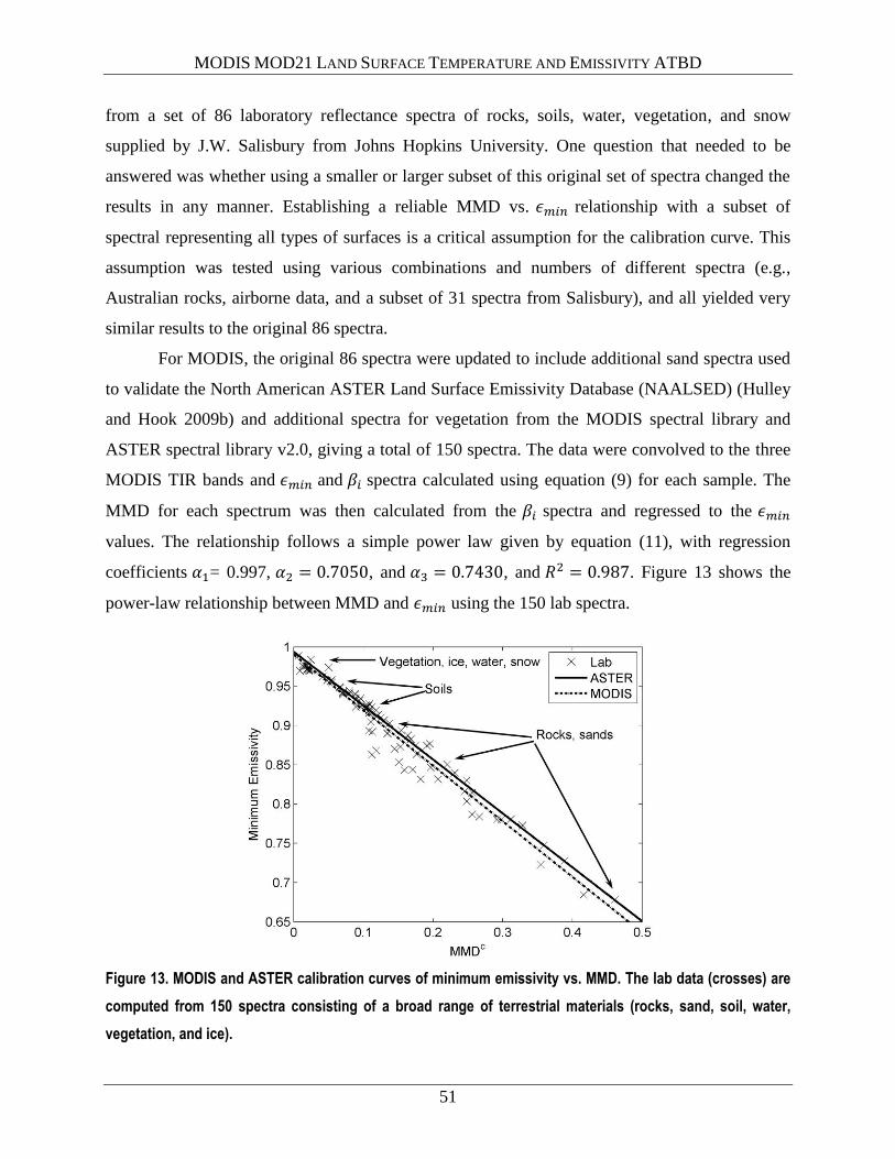
MODIS MOD21 LAND SURFACE TEMPERATURE AND EMISSIVITY ATBD
51
from a set of 86 laboratory reflectance spectra of rocks, soils, water, vegetation, and snow
supplied by J.W. Salisbury from Johns Hopkins University. One question that needed to be
answered was whether using a smaller or larger subset of this original set of spectra changed the
results in any manner. Establishing a reliable MMD vs. relationship with a subset of
spectral representing all types of surfaces is a critical assumption for the calibration curve. This
assumption was tested using various combinations and numbers of different spectra (e.g.,
Australian rocks, airborne data, and a subset of 31 spectra from Salisbury), and all yielded very
similar results to the original 86 spectra.
For MODIS, the original 86 spectra were updated to include additional sand spectra used
to validate the North American ASTER Land Surface Emissivity Database (NAALSED) (Hulley
and Hook 2009b) and additional spectra for vegetation from the MODIS spectral library and
ASTER spectral library v2.0, giving a total of 150 spectra. The data were convolved to the three
MODIS TIR bands and and 𝛽 spectra calculated using equation (9) for each sample. The
MMD for each spectrum was then calculated from the 𝛽 spectra and regressed to the
values. The relationship follows a simple power law given by equation (11), with regression
coefficients = 0.997, , and , and . Figure 13 shows the
power-law relationship between MMD and using the 150 lab spectra.
Figure 13. MODIS and ASTER calibration curves of minimum emissivity vs. MMD. The lab data (crosses) are
computed from 150 spectra consisting of a broad range of terrestrial materials (rocks, sand, soil, water,
vegetation, and ice).
MODIS MOD21 LAND SURFACE TEMPERATURE AND EMISSIVITY ATBD
52
6.2.10 Atmospheric Effects
The accuracy of the atmospheric correction technique used to estimate the surface
radiance relies on the accuracy of the variables input to the radiative transfer model (e.g., air
temperature, relative humidity, and ozone). A sensitivity analysis has shown (Table 1) that a
change in atmospheric water vapor of 20% leads to a 4.43% change in radiance for MODIS band
12 (12 µm), which is the most susceptible to atmospheric absorption and emission of the three
MODIS TIR bands, while a change in air temperature of 2 K leads to a 1.6% change in
radiance for a tropical atmosphere. Changes in ozone and aerosol amount had much smaller
effects, except for MODIS band 29 (8.55 µm), which falls closer to the ozone absorption region
at 9.6 µm. These atmospheric errors tend to be highly correlated from band to band, since each
channel has a characteristic absorbing feature. As a result, the effect on TES output is usually
relatively small, but if these errors are uncorrelated from band to band then much larger errors
can occur, particularly for graybodies, where small changes in MMD can significantly alter the
shape of the emissivity spectrum. For example, over water bodies, errors in emissivity of up to
3% (0.03) have been found due to uncompensated atmospheric effects (Hulley and Hook 2009b;
Tonooka and Palluconi 2005).
One method for improving the accuracy of the surface radiance product is to apply the
WVS method (Tonooka 2005). Using 183 ASTER scenes over lakes, rivers, and sea surfaces, it
was found that using the WVS method instead of the standard atmospheric correction improved
estimates of surface temperature from 3 to 8 K in regions of high humidity (Tonooka 2005).
These are substantial errors when considering that the required accuracy of the TES algorithm is
~1 K (Gillespie et al. 1998).
Figure 14 shows emissivity spectra over the Salton Sea, showing the effects of applying
the WVS atmospheric correction method on the shape of the emissivity spectrum when
compared to using the standard (STD) correction method without WVS. The emissivity spectrum
of water is high (~0.98) and flat and the results in Figure 14 show a dramatic improvement in
emissivity accuracy in both magnitude (up to 0.06 for ASTER band 11, and 0.09 for MODIS
band 29) and spectral shape when using the WVS as opposed to the STD method. Because of the
humid day, where MOD07 precipitable water vapor (PWV) values were around 4 cm over the
water, the spectral contrast of the STD emissivity results are overestimated for ASTER and
MODIS data. However, when applying the WVS method, the ASTER emissivity spectra fall
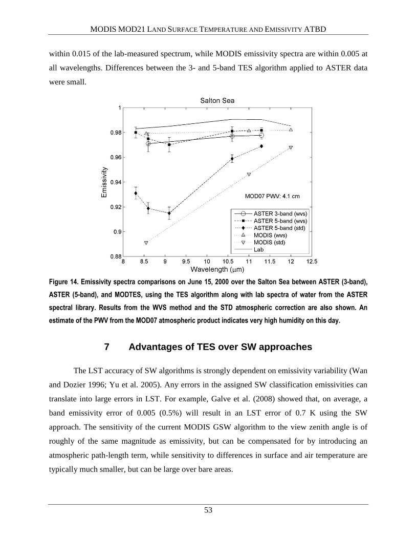
MODIS MOD21 LAND SURFACE TEMPERATURE AND EMISSIVITY ATBD
53
within 0.015 of the lab-measured spectrum, while MODIS emissivity spectra are within 0.005 at
all wavelengths. Differences between the 3- and 5-band TES algorithm applied to ASTER data
were small.
Figure 14. Emissivity spectra comparisons on June 15, 2000 over the Salton Sea between ASTER (3-band),
ASTER (5-band), and MODTES, using the TES algorithm along with lab spectra of water from the ASTER
spectral library. Results from the WVS method and the STD atmospheric correction are also shown. An
estimate of the PWV from the MOD07 atmospheric product indicates very high humidity on this day.
7 Advantages of TES over SW approaches
The LST accuracy of SW algorithms is strongly dependent on emissivity variability (Wan
and Dozier 1996; Yu et al. 2005). Any errors in the assigned SW classification emissivities can
translate into large errors in LST. For example, Galve et al. (2008) showed that, on average, a
band emissivity error of 0.005 (0.5%) will result in an LST error of 0.7 K using the SW
approach. The sensitivity of the current MODIS GSW algorithm to the view zenith angle is of
roughly of the same magnitude as emissivity, but can be compensated for by introducing an
atmospheric path-length term, while sensitivity to differences in surface and air temperature are
typically much smaller, but can be large over bare areas.
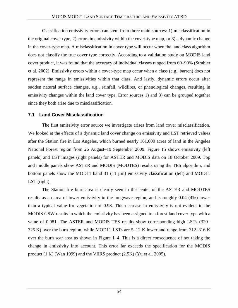
MODIS MOD21 LAND SURFACE TEMPERATURE AND EMISSIVITY ATBD
54
Classification emissivity errors can stem from three main sources: 1) misclassification in
the original cover type, 2) errors in emissivity within the cover-type map, or 3) a dynamic change
in the cover-type map. A misclassification in cover type will occur when the land class algorithm
does not classify the true cover type correctly. According to a validation study on MODIS land
cover product, it was found that the accuracy of individual classes ranged from 60–90% (Strahler
et al. 2002). Emissivity errors within a cover-type map occur when a class (e.g., barren) does not
represent the range in emissivities within that class. And lastly, dynamic errors occur after
sudden natural surface changes, e.g., rainfall, wildfires, or phenological changes, resulting in
emissivity changes within the land cover type. Error sources 1) and 3) can be grouped together
since they both arise due to misclassification.
7.1 Land Cover Misclassification
The first emissivity error source we investigate arises from land cover misclassification.
We looked at the effects of a dynamic land cover change on emissivity and LST retrieved values
after the Station fire in Los Angeles, which burned nearly 161,000 acres of land in the Angeles
National Forest region from 26 August–19 September 2009. Figure 15 shows emissivity (left
panels) and LST images (right panels) for ASTER and MODIS data on 10 October 2009. Top
and middle panels show ASTER and MODIS (MODTES) results using the TES algorithm, and
bottom panels show the MOD11 band 31 (11 µm) emissivity classification (left) and MOD11
LST (right).
The Station fire burn area is clearly seen in the center of the ASTER and MODTES
results as an area of lower emissivity in the longwave region, and is roughly 0.04 (4%) lower
than a typical value for vegetation of 0.98. This decrease in emissivity is not evident in the
MODIS GSW results in which the emissivity has been assigned to a forest land cover type with a
value of 0.981. The ASTER and MODIS TES results show corresponding high LSTs (320–
325 K) over the burn region, while MOD11 LSTs are 5–12 K lower and range from 312–316 K
over the burn scar area as shown in Figure 1–4. This is a direct consequence of not taking the
change in emissivity into account. This error far exceeds the specification for the MODIS
product (1 K) (Wan 1999) and the VIIRS product (2.5K) (Yu et al. 2005).
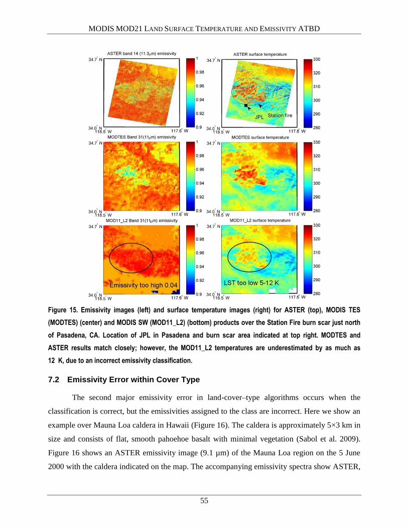
MODIS MOD21 LAND SURFACE TEMPERATURE AND EMISSIVITY ATBD
55
Figure 15. Emissivity images (left) and surface temperature images (right) for ASTER (top), MODIS TES
(MODTES) (center) and MODIS SW (MOD11_L2) (bottom) products over the Station Fire burn scar just north
of Pasadena, CA. Location of JPL in Pasadena and burn scar area indicated at top right. MODTES and
ASTER results match closely; however, the MOD11_L2 temperatures are underestimated by as much as
12 K, due to an incorrect emissivity classification.
7.2 Emissivity Error within Cover Type
The second major emissivity error in land-cover–type algorithms occurs when the
classification is correct, but the emissivities assigned to the class are incorrect. Here we show an
example over Mauna Loa caldera in Hawaii (Figure 16). The caldera is approximately 5×3 km in
size and consists of flat, smooth pahoehoe basalt with minimal vegetation (Sabol et al. 2009).
Figure 16 shows an ASTER emissivity image (9.1 µm) of the Mauna Loa region on the 5 June
2000 with the caldera indicated on the map. The accompanying emissivity spectra show ASTER,
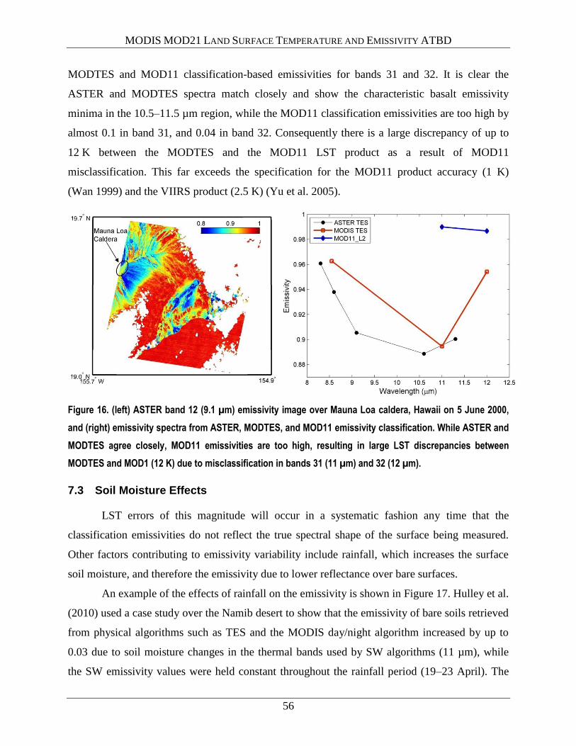
MODIS MOD21 LAND SURFACE TEMPERATURE AND EMISSIVITY ATBD
56
MODTES and MOD11 classification-based emissivities for bands 31 and 32. It is clear the
ASTER and MODTES spectra match closely and show the characteristic basalt emissivity
minima in the 10.5–11.5 µm region, while the MOD11 classification emissivities are too high by
almost 0.1 in band 31, and 0.04 in band 32. Consequently there is a large discrepancy of up to
12 K between the MODTES and the MOD11 LST product as a result of MOD11
misclassification. This far exceeds the specification for the MOD11 product accuracy (1 K)
(Wan 1999) and the VIIRS product (2.5 K) (Yu et al. 2005).
Figure 16. (left) ASTER band 12 (9.1 µm) emissivity image over Mauna Loa caldera, Hawaii on 5 June 2000,
and (right) emissivity spectra from ASTER, MODTES, and MOD11 emissivity classification. While ASTER and
MODTES agree closely, MOD11 emissivities are too high, resulting in large LST discrepancies between
MODTES and MOD1 (12 K) due to misclassification in bands 31 (11 µm) and 32 (12 µm).
7.3 Soil Moisture Effects
LST errors of this magnitude will occur in a systematic fashion any time that the
classification emissivities do not reflect the true spectral shape of the surface being measured.
Other factors contributing to emissivity variability include rainfall, which increases the surface
soil moisture, and therefore the emissivity due to lower reflectance over bare surfaces.
An example of the effects of rainfall on the emissivity is shown in Figure 17. Hulley et al.
(2010) used a case study over the Namib desert to show that the emissivity of bare soils retrieved
from physical algorithms such as TES and the MODIS day/night algorithm increased by up to
0.03 due to soil moisture changes in the thermal bands used by SW algorithms (11 µm), while
the SW emissivity values were held constant throughout the rainfall period (19–23 April). The
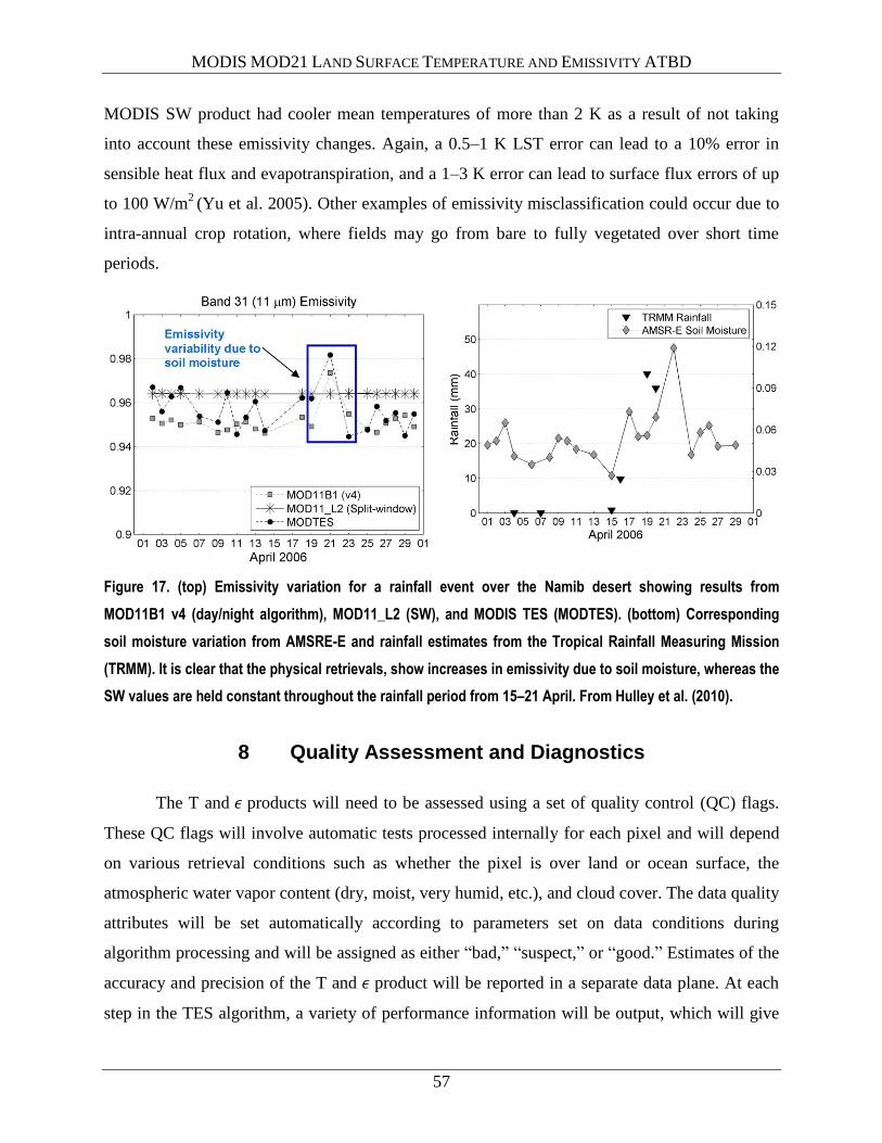
MODIS MOD21 LAND SURFACE TEMPERATURE AND EMISSIVITY ATBD
57
MODIS SW product had cooler mean temperatures of more than 2 K as a result of not taking
into account these emissivity changes. Again, a 0.5–1 K LST error can lead to a 10% error in
sensible heat flux and evapotranspiration, and a 1–3 K error can lead to surface flux errors of up
to 100 W/m2 (Yu et al. 2005). Other examples of emissivity misclassification could occur due to
intra-annual crop rotation, where fields may go from bare to fully vegetated over short time
periods.
Figure 17. (top) Emissivity variation for a rainfall event over the Namib desert showing results from
MOD11B1 v4 (day/night algorithm), MOD11_L2 (SW), and MODIS TES (MODTES). (bottom) Corresponding
soil moisture variation from AMSRE-E and rainfall estimates from the Tropical Rainfall Measuring Mission
(TRMM). It is clear that the physical retrievals, show increases in emissivity due to soil moisture, whereas the
SW values are held constant throughout the rainfall period from 15–21 April. From Hulley et al. (2010).
8 Quality Assessment and Diagnostics
The T and products will need to be assessed using a set of quality control (QC) flags.
These QC flags will involve automatic tests processed internally for each pixel and will depend
on various retrieval conditions such as whether the pixel is over land or ocean surface, the
atmospheric water vapor content (dry, moist, very humid, etc.), and cloud cover. The data quality
attributes will be set automatically according to parameters set on data conditions during
algorithm processing and will be assigned as either “bad,” “suspect,” or “good.” Estimates of the
accuracy and precision of the T and product will be reported in a separate data plane. At each
step in the TES algorithm, a variety of performance information will be output, which will give

MODIS MOD21 LAND SURFACE TEMPERATURE AND EMISSIVITY ATBD
58
the user a summary of algorithm statistics in a spatial context. This type of information will be
useful for determining surface type, atmospheric conditions, and overall performance of TES.
The architecture of the MODIS T and QA data plane will closely resemble that of
ASTER (Gillespie et al. 1998). It will consist of header information followed by three 8-bit QA
data planes. The structure of the first QA data plane will consist of three primary fields, which
are detailed in Table 6:
1. Data Quality Field: “bad,” “suspect,” or “good,” to be assigned to specific bit patterns.
2. Cloud Mask Field: Outputs from cloud mask statistics, e.g., optically thick or thin cloud,
cirrus or contrails, clear, or snow/ice determined from NDSI threshold.
3. Cloud Adjacency: Clear pixels defined in the cloud mask will be assigned an adjacency
category dependent on distance to the nearest cloud defined quantitatively by the number of
pixels (e.g., very close, close, far, very far).
The structure of the second QA data plane will consist of performance metrics output
from various stages of the TES algorithm, detailed in Table 7:
1. The final value of used in the NEM module after optimization (if necessary).
2. Number of iterations needed to remove reflected downwelling sky irradiance.
3. Atmospheric opacity test for humid scenes, using test.
4. MMD regime: MMD < 0.3 (near-graybody) or MMD > 0.3 (likely bare).
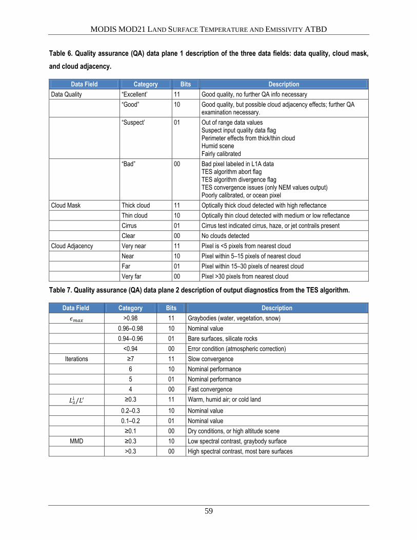
MODIS MOD21 LAND SURFACE TEMPERATURE AND EMISSIVITY ATBD
59
Table 6. Quality assurance (QA) data plane 1 description of the three data fields: data quality, cloud mask,
and cloud adjacency.
Data Field Category Bits Description
Data Quality “Excellent’ 11 Good quality, no further QA info necessary
“Good” 10 Good quality, but possible cloud adjacency effects; further QA examination necessary.
“Suspect’ 01 Out of range data values Suspect input quality data flag Perimeter effects from thick/thin cloud Humid scene Fairly calibrated
“Bad” 00 Bad pixel labeled in L1A data TES algorithm abort flag TES algorithm divergence flag TES convergence issues (only NEM values output) Poorly calibrated, or ocean pixel
Cloud Mask Thick cloud 11 Optically thick cloud detected with high reflectance
Thin cloud 10 Optically thin cloud detected with medium or low reflectance
Cirrus 01 Cirrus test indicated cirrus, haze, or jet contrails present
Clear 00 No clouds detected
Cloud Adjacency Very near 11 Pixel is <5 pixels from nearest cloud
Near 10 Pixel within 5–15 pixels of nearest cloud
Far 01 Pixel within 15–30 pixels of nearest cloud
Very far 00 Pixel >30 pixels from nearest cloud
Table 7. Quality assurance (QA) data plane 2 description of output diagnostics from the TES algorithm.
Data Field Category Bits Description
>0.98 11 Graybodies (water, vegetation, snow)
0.96–0.98 10 Nominal value
0.94–0.96 01 Bare surfaces, silicate rocks
<0.94 00 Error condition (atmospheric correction)
Iterations ≥7 11 Slow convergence
6 10 Nominal performance
5 01 Nominal performance
4 00 Fast convergence
≥0.3 11 Warm, humid air; or cold land
0.2–0.3 10 Nominal value
0.1–0.2 01 Nominal value
≥0.1 00 Dry conditions, or high altitude scene
MMD ≥0.3 10 Low spectral contrast, graybody surface
>0.3 00 High spectral contrast, most bare surfaces
MODIS MOD21 LAND SURFACE TEMPERATURE AND EMISSIVITY ATBD
60
9 Uncertainty Analysis
NASA has identified a major need to develop long-term, consistent products valid across
multiple missions, with well-defined uncertainty statistics addressing specific Earth-science
questions. These products are termed Earth System Data Records (ESDRs), and LST&E has
been identified as an important ESDR. Currently a lack of understanding of LST&E uncertainties
limits their usefulness in land surface and climate models. In this section we present results from
an LST&E uncertainty simulator that has been developed to quantify and model uncertainties for
a variety of TIR sensors and LST algorithms (Hulley et al. 2012). Using the simulator,
uncertainties were estimated for the MOD21 LST&E product, including WVS. These
uncertainties are parameterized according to view angle and estimated total column water vapor
for application to real MODIS data.
9.1 The Temperature and Emissivity Uncertainty Simulator
A Temperature Emissivity Uncertainty Simulator (TEUSim) has been developed for
simulating LST&E uncertainties from various sources of error for the TES and SW algorithms in
a rigorous manner for any appropriate TIR sensor. These include random errors (noise),
systematic errors (calibration), and spatio-temporally correlated errors (atmospheric). The
MODTRAN 5.2 radiative transfer model is used for the simulations with a global set of
radiosonde profiles and surface emissivity spectra representing a broad range of atmospheric
conditions and a wide variety of surface types. This approach allows the retrieval algorithm to be
easily evaluated under realistic but challenging combinations of surface/atmospheric conditions.
The TEUSim is designed to separately quantify error contributions from the following potential
sources:
Noise
Model
Atmospheric correction
Undetected cloud
Calibration
The results presented in this study will focus on the first three of these error sources: noise,
model, and atmosphere.
MODIS MOD21 LAND SURFACE TEMPERATURE AND EMISSIVITY ATBD
61
9.2 Atmospheric Profiles
The TEUSim uses a global set of atmospheric radiosoundings constructed from the
University of Wyoming Atmospheric Science Department’s CLAR database (Galve et al. 2008).
CLAR contains 382 globally distributed radiosoundings for both day and night in 65 layers from
the surface to 100 km. The CLAR database includes a wide range of TCW estimates up to 7 cm
and surface air temperature ranging from 20º C to 40º C. Radiosondes acquired from 2003 to
2006 were distributed over three latitude ranges (40% from 0º–30º, 40% from 30º–60º, 20%
above 60º) and screened for cloud and fog contamination using a procedure described by
Francois et al. (2002).
9.3 Radiative Transfer Model
In TEUSim the latest version of MODTRAN (v5.2) was used for the radiative transfer
calculations. MODTRAN 5.2 uses an improved molecular band model, termed the Spectrally
Enhanced Resolution MODTRAN (SERTRAN), which has a much finer spectroscopy (0.1 cm-1
)
than previous versions (1–2 cm-1
). This results in higher accuracy in modeling of band
absorption features in the longwave TIR window regions, and comparisons with line-by-line
models has shown good accuracy (Berk et al. 2005).
9.4 Surface End-Member Selection
A selection of emissivity spectra from the ASTER Spectral Library v2.0 (ASTlib)
(Baldridge et al. 2009) were used to define the surface spectral emission term in MODTRAN. A
total of 59 spectra were chosen based on certain criteria and grouped into four surface
classifications: rocks (20), soils (26), sands (9), and graybodies (4). The doublets between 8–
9.5 µm and 12.5–13 µm are the result of Si-O stretching, and the exact position of the feature at
11.2 µm is dependent on the size of the cation paired with the carbonate (CO3) molecule. Spectra
were chosen to represent the most realistic effective emissivities observed at the remote sensing
scales of ASTER (90 m) and MODIS (1 km) using the following methodology.
For rocks, certain spectra were removed prior to processing based on two considerations.
First, samples that rarely exist as kilometer-scale, sub-aerial end-member exposures on the
Earth’s surface such as pyroxenite or serpentinite were eliminated. Second, and in parallel,
spectrally similar samples were eliminated. Spectral similarity was defined by the location,
MODIS MOD21 LAND SURFACE TEMPERATURE AND EMISSIVITY ATBD
62
shape, and magnitude of spectral features between 7 and 13 µm. All eliminated samples are
represented in the final selection through spectrally-similar end-member types. The final rock set
included 20 spectra.
ASTlib includes 49 soil spectra classified according to their taxonomy, such as Alfisol
(9), Aridisol (14), Entisol (10), Inceptisol (7) and Mollisol (9). Filtering in this case was based
solely on spectral similarity between each taxonomy type. The final soils set included 26 soil
spectra.
A set of nine emissivity spectra collected in separate field campaigns during 2008 over
large homogeneous sand dune sites in the southwestern United States in support of validation for
the NAALSED v2.0 (Hulley et al. 2009a) were used for sands. The sand samples consist of a
wide variety of different minerals including quartz, magnetite, feldspars, gypsum, and basalt
mixed in various amounts, and represent a broad range of emissivities in the TIR as detailed in
Hulley et al. (2009a).
To represent graybody surfaces, spectra of distilled water, ice, snow, and conifer were
chosen from ASTlib. Four spectra were sufficient to represent this class since graybody surfaces
exhibit low contrast and high emissivities. It should be noted that certain types of man-made
materials were not included, such as aluminum roofs that do not occur at the spatial resolution of
these sensors, but should be included for higher-spatial-resolution data sets such as those
provided by airborne instruments.
9.5 Radiative Transfer Simulations
In the TEUSim, each CLAR radiosonde profile for each set of end-member spectra was
used as an input to MODTRAN 5.2. A seasonal rural aerosol was assumed with standard profiles
for fixed gases within MODTRAN. For MODIS, five viewing angles were used, representing the
Gaussian angles proposed by Wan and Dozier (1996): 0°, 11.6°, 26.1°, 40.3°, and 53.7°. In the
WVS simulation model, the downward sky irradiance, ( ), can be modeled using the path
radiance, transmittance, and view angle. To simulate the downward sky irradiance in
MODTRAN, the sensor target is placed a few meters above the surface, with surface emission
set to zero, and view angle set at the prescribed angles above. In this configuration, the reflected
downwelling sky irradiance is estimated for a given view angle. The total sky irradiance

MODIS MOD21 LAND SURFACE TEMPERATURE AND EMISSIVITY ATBD
63
contribution for band i is then calculated by summing the contribution of all view angles over the
entire hemisphere:
(24)
where is the view angle and is the azimuth angle. To minimize computational time, the
downward sky irradiance is first modeled as a non-linear function of path radiance at nadir view
using (1) (Tonooka 2001):
(25)
where , , and are regression coefficients, and is computed by:
(26)
Equations (2) and (3) were used to estimate the downwelling sky irradiance in the TEUSim
results using pre-calculated regression coefficients for MODIS bands 29, 31, and 32. The
reflected sky irradiance term is generally smaller in magnitude than the surface-emitted radiance,
but needs to be taken into account, particularly on humid days when the total atmospheric water
vapor content is high. The simulated LST is based on the surface air temperature in the CLAR
database as follows:
(27)
where and are the simulated LST and surface air temperature. Galve et al. (2008)
found a mean of +3 K and standard deviation of 9 K from a global study of surface-air
temperature differences over land in the MODIS MOD08 and MOD11 products. We therefore
defined as a random distribution with a mean of 3 K and a standard deviation of 9 K for each
profile input to MODTRAN.
The TES algorithm uses surface radiance as input, which can be derived from the
atmospheric transmittance ( ), TOA radiance ( ), path radiance ( ), and downward sky
irradiance ( ). To calculate the various sources of error in LST&E retrievals from TES, these
variables were simulated for the following conditions:
1. Perfect atmosphere (i.e., exact inputs): ( ) and atmospheric parameters ( ), ( ), and
( ) calculated using a given profile, surface type and viewing angle;
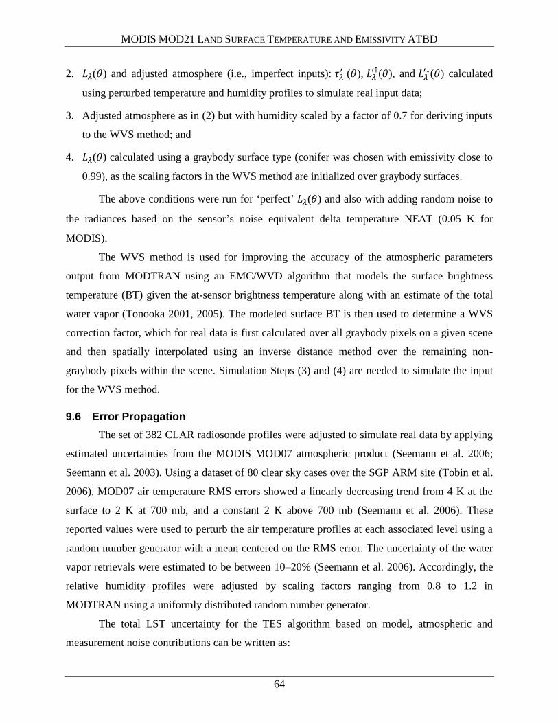
MODIS MOD21 LAND SURFACE TEMPERATURE AND EMISSIVITY ATBD
64
2. ( ) and adjusted atmosphere (i.e., imperfect inputs): ( ),
( ), and ( ) calculated
using perturbed temperature and humidity profiles to simulate real input data;
3. Adjusted atmosphere as in (2) but with humidity scaled by a factor of 0.7 for deriving inputs
to the WVS method; and
4. ( ) calculated using a graybody surface type (conifer was chosen with emissivity close to
0.99), as the scaling factors in the WVS method are initialized over graybody surfaces.
The above conditions were run for ‘perfect’ ( ) and also with adding random noise to
the radiances based on the sensor’s noise equivalent delta temperature NET (0.05 K for
MODIS).
The WVS method is used for improving the accuracy of the atmospheric parameters
output from MODTRAN using an EMC/WVD algorithm that models the surface brightness
temperature (BT) given the at-sensor brightness temperature along with an estimate of the total
water vapor (Tonooka 2001, 2005). The modeled surface BT is then used to determine a WVS
correction factor, which for real data is first calculated over all graybody pixels on a given scene
and then spatially interpolated using an inverse distance method over the remaining non-
graybody pixels within the scene. Simulation Steps (3) and (4) are needed to simulate the input
for the WVS method.
9.6 Error Propagation
The set of 382 CLAR radiosonde profiles were adjusted to simulate real data by applying
estimated uncertainties from the MODIS MOD07 atmospheric product (Seemann et al. 2006;
Seemann et al. 2003). Using a dataset of 80 clear sky cases over the SGP ARM site (Tobin et al.
2006), MOD07 air temperature RMS errors showed a linearly decreasing trend from 4 K at the
surface to 2 K at 700 mb, and a constant 2 K above 700 mb (Seemann et al. 2006). These
reported values were used to perturb the air temperature profiles at each associated level using a
random number generator with a mean centered on the RMS error. The uncertainty of the water
vapor retrievals were estimated to be between 10–20% (Seemann et al. 2006). Accordingly, the
relative humidity profiles were adjusted by scaling factors ranging from 0.8 to 1.2 in
MODTRAN using a uniformly distributed random number generator.
The total LST uncertainty for the TES algorithm based on model, atmospheric and
measurement noise contributions can be written as:

MODIS MOD21 LAND SURFACE TEMPERATURE AND EMISSIVITY ATBD
65
(28)
where is the model error due to assumptions made in the TES calibration curve, is
the atmospheric error, and is the error associated with measurement noise. These errors
are assumed to be independent.
To calculate the separate contributions from each of these errors let us first denote the
simulated atmospheric parameters as x ,
] and simulated observed radiance
parameter as . Both and are required to estimate the surface radiance that is input
to the TES algorithm. In reality, however, the input parameters are not known explicitly, but
are associated with some error, , which we write as . Similarly, the observed
radiances have an associated noise based on the NET of the specific sensor, which we will
denote by . To characterize the model error, we express the TES algorithm as a function based
on perfect input parameters and such that ). The model error, , i.e.,
due to assumptions in the TES algorithm alone, can then be written as:
(29)
where is the simulated LST used in the MODTRAN simulations, and denotes
the mean-square error between the retrieved and simulated LST for inputs and . The
atmospheric error can be written as the difference between TES using perfect atmospheric inputs,
and imperfect inputs, :
(30)
And lastly the error due to measurement noise can be written as the difference between TES with
perfect simulated TOA radiances, and TES with noisy radiances, :
(31)
Since the TES algorithm simultaneously retrieves the LST and spectral emissivity, the above
equations also apply to the corresponding emissivity retrieval for each band.
The effects of sensor view angle on the accuracy of MODIS TES retrievals of LST are
shown in Figure 18. LST uncertainties are plotted against TCW for four simulated Gaussian
view angles of 0°, 26.1°, 40.3°, and 53.7°. It is clear that the uncertainties become larger with
both TCW and view angle; however, this is due to TCW in both cases. A TCW amount of 4 cm
at a 53.7° view angle has an effective TCW of 6.2 cm, due to an increase in atmospheric path
length increases by a factor of cos-1
(53.7°). The LSTs are underestimated at higher view angles
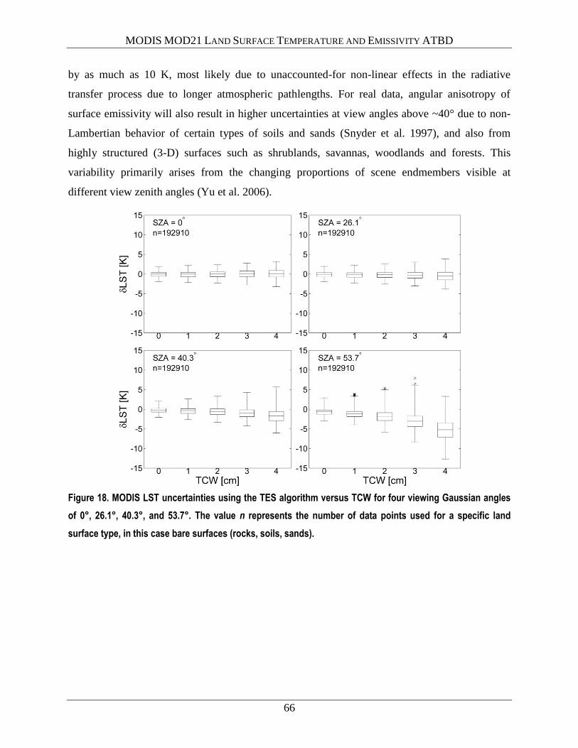
MODIS MOD21 LAND SURFACE TEMPERATURE AND EMISSIVITY ATBD
66
by as much as 10 K, most likely due to unaccounted-for non-linear effects in the radiative
transfer process due to longer atmospheric pathlengths. For real data, angular anisotropy of
surface emissivity will also result in higher uncertainties at view angles above ~40° due to non-
Lambertian behavior of certain types of soils and sands (Snyder et al. 1997), and also from
highly structured (3-D) surfaces such as shrublands, savannas, woodlands and forests. This
variability primarily arises from the changing proportions of scene endmembers visible at
different view zenith angles (Yu et al. 2006).
Figure 18. MODIS LST uncertainties using the TES algorithm versus TCW for four viewing Gaussian angles
of 0°, 26.1°, 40.3°, and 53.7°. The value n represents the number of data points used for a specific land
surface type, in this case bare surfaces (rocks, soils, sands).

MODIS MOD21 LAND SURFACE TEMPERATURE AND EMISSIVITY ATBD
67
9.7 Parameterization of Uncertainties
A key requirement for generating LST&E ESDR from either multiple sensors or
algorithms is accurate knowledge of uncertainties from the contributing products. Uncertainties
for each input product must be rigorously estimated for a variety of different conditions on a
pixel-by-pixel basis before they can be merged and incorporated into a time series of
measurements of sufficient length, consistency, and continuity to adequately meet the science
requirements of an ESDR. Current LST&E datasets are available with quality control
information, but do not include a full set of uncertainty statistics. For example, the standard
ASTER and MODIS LST product QC data planes specify qualitative uncertainty information,
and MODIS includes a rough estimate of LST&E error, but no uncertainty data-planes exist on a
pixel-by-pixel basis dependent upon factors such as land cover type, view angle, and total
column water vapor.
The next logical step is to apply the uncertainty statistics produced from the TEUSim to
real data from MOD21 retrievals. To achieve this the total uncertainty, taken as the RMSE of the
differences between simulated (truth) and retrieved LST&E including atmospheric error, was
modeled according to view angle, total water vapor column amount, and land surface type using
a least-squares method fit to a quadratic function. Three surface types were classified: graybody,
transitional, and bare. The transitional surface represents a mixed cover type, and was calculated
by varying the vegetation fraction cover percentage, , by 25, 50, and 75% for the set of bare
surface spectra (rocks, soils, sand) as follows:
(32)
where is the transition emissivity, is a graybody emissivity spectrum (e.g., conifer),
and are the lab emissivities for bare surfaces.
For MODIS, the total uncertainty includes both a sensor view angle (SVA) and TCW
dependence. The total uncertainty for MODIS LST can be expressed as:
𝑉 𝑉
(33)
Similarly, the band-dependent emissivity uncertainties can be expressed as:
𝑉 𝑉
(34)
where is the LST uncertainty (K) calculated as the difference between the simulated and
retrieved LST, is the band-dependent emissivity uncertainty for band i, calculated as the
MODIS MOD21 LAND SURFACE TEMPERATURE AND EMISSIVITY ATBD
68
difference between the input lab emissivity and retrieved emissivity, and and are the LST
and emissivity regression coefficients and depend on surface type (graybody, transition, bare).
A sensitivity study showed that the parameterizations given by equations 10–13 provided
the best fit to the simulation results in terms of RMSE, with fits of ~0.1 K. Once the coefficients
are established they can be applied on a pixel-by-pixel basis across any scene given estimates of
TCW from either a retrieval (e.g., MODIS MOD07 or AIRS) or a numerical weather model (e.g.,
ECMWF, NCEP), and the SVA from the product metadata. A simple emissivity threshold using a
band with large spectral variation can be used to discriminate between graybody, transition, and
bare types in any given scene for application of the relevant coefficients.
Figure 19(a) shows the retrieved LST using the TES algorithm with WVS correction and
corresponding uncertainty in Figure 19(c), while Figure 19(b) shows the retrieved emissivity for
band 29 and corresponding uncertainty in Figure 19(d). The highest LST uncertainties range
from 2–3 K in the monsoonal region to over 5 K on the edges of cloudy regions, where
uncertainties are highest as expected. Over most of the scene where TCW values are <2 cm, the
LST uncertainties are generally <1.5 K. Similar to the LST results, the uncertainties in band 29
emissivity are highest over the monsoonal region, ranging from 0.03–0.05, and along the edges
of clouds. Over drier regions of California and Nevada, there is a stronger uncertainty correlation
with cover type, with lowest uncertainties over the denser forests of the Sierra Nevadas (~0.015)
and slightly higher over bare and mixed regions (~0.02). For this scene, retrievals were restricted
to view angles <40º, so uncertainty dependencies related to view angle are not evident; however,
at angles >40º the uncertainties for both LST and emissivity increase noticeably due to reasons
discussed earlier.
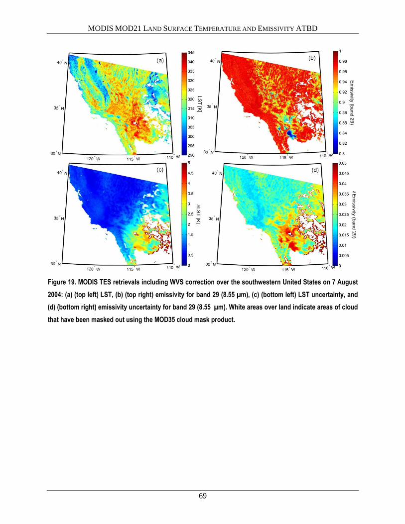
MODIS MOD21 LAND SURFACE TEMPERATURE AND EMISSIVITY ATBD
69
Figure 19. MODIS TES retrievals including WVS correction over the southwestern United States on 7 August
2004: (a) (top left) LST, (b) (top right) emissivity for band 29 (8.55 µm), (c) (bottom left) LST uncertainty, and
(d) (bottom right) emissivity uncertainty for band 29 (8.55 µm). White areas over land indicate areas of cloud
that have been masked out using the MOD35 cloud mask product.
MODIS MOD21 LAND SURFACE TEMPERATURE AND EMISSIVITY ATBD
70
10 Validation
Two methods have been established for validating MODIS LST data: a conventional T-
based method and an R-based method (Wan and Li 2008). The T-based method requires ground
measurements over thermally homogenous sites concurrent with the satellite overpass, while the
R-based method relies on a radiative closure simulation in a clear atmospheric window region to
estimate the LST from top of atmosphere (TOA) observed brightness temperatures, assuming the
emissivity is known from ground measurements. The T-based method is the preferred method,
but it requires accurate in-situ measurements that are only available from a small number of
thermally homogeneous sites concurrently with the satellite overpass. The R-based method is not
a true validation in the classical sense, but it does not require simultaneous in-situ measurements
and is therefore easier to implement both day and night over a larger number of global sites;
however, it is susceptible to errors in the atmospheric correction and emissivity uncertainties.
The MOD11_L2 LST product has been validated with a combination of T-based and R-based
methods over more than 19 types of thermally homogenous surfaces including lakes (Hook et al.
2007), dedicated field campaign sites over agricultural fields and forests (Coll et al. 2005),
playas and grasslands (Wan et al. 2004; Wan 2008), and for a range of different seasons and
years. LST errors are generally within ±1 K for all sites under stable atmospheric conditions
except semi-arid and arid areas, which had errors of up to 5 K (Wan and Li 2008).
Initial testing and validation of the MOD21 emissivity product has shown good
agreement with the North American ASTER Land Surface Database (NAALSED) v2.0
emissivity product (Hulley et al. 2009a) and in-situ data over nine pseudo-invariant sand dune
sites in the southwestern United States to <0.02 (2%) (Hulley and Hook 2011). NAALSED was
validated over arid/semi-arid regions using nine pseudo-invariant sand dune sites in the
western/southwestern United States. The emissivity of samples collected at each of the nine sites
was determined in the laboratory using a Nicolet 520 FT-IR spectrometer and convolved with the
appropriate ASTER system response functions. Validation of emissivity data from space ideally
requires a site that is homogeneous in emissivity at the scale of the imagery, allowing several
image pixels to be validated over the target site. The nine sand dune validation sites chosen for
the ASTER study and planned for use with the MOD21 product are: Great Sands National Park,
Colorado; White Sands National Monument, New Mexico; Kelso Dunes, California; Algodones

MODIS MOD21 LAND SURFACE TEMPERATURE AND EMISSIVITY ATBD
71
Dunes, California; Stovepipe Wells Dunes, California; Coral Pink Sand Dunes, Utah; Little
Sahara Dunes, Utah; Killpecker Dunes, Wyoming; and Moses Lake Basalt Dunes, Washington.
A validation study at the Land Surface Analysis–Satellite Application Facility (LSA-
SAF) Gobabeb validation site in Namibia showed that MOD21 LSEs matched closely with in-
situ emissivity data (~1%), while emissivities based on land cover classification products (e.g.,
SEVIRI, MOD11) overestimated emissivities over the sand dunes by as much as 3.5% (Gottsche
and Hulley 2012). R-based validation of the MOD21 product is currently underway over nine
pseudo-invariant sites in southwestern United States, and the Lake Tahoe and Salton Sea cal/val
sites.
For the MOD21 product we plan to use in-situ data from a variety of ground sites
covering the majority of different land-cover types defined in the International Geosphere-
Biosphere Programme (IGBP). The sites will consist of water, vegetation (forest, grassland, and
crops), and barren areas (Table 8).
Table 8. The core set of global validation sites according to IGBP class to be used for validation and
calibration of the MODIS MOD21 land surface temperature and emissivity product.
10.1 Water Sites
For water surfaces, we will use the Lake Tahoe, California/Nevada, automated validation
site where measurements of skin temperature have been made every two minutes since 1999 and
are used to validate the mid and thermal infrared data and products from ASTER and MODIS
(Hook et al. 2007). Water targets are ideal for cal/val activities because they are thermally
homogeneous and the emissivity is generally well known. A further advantage of Tahoe is that
the lake is located at high altitude, which minimizes atmospheric correction errors, and is large
IGBP Class Sites
0 Water Tahoe, Salton Sea, CA
1,2 Needle-leaf forest Krasnoyarsk, Russia; Tharandt, Germany; Fairhope, Alaska
3,4,5 Broad-leaf/mixed forest Chang Baisan, China; Hainich, Germany; Hilo, Hawaii
6,7 Open/closed shrublands Desert Rock, NV; Stovepipe Wells, CA
8,9,10 Savannas/Grasslands Boulder, CO; Fort Peck, MT
12 Croplands Bondville, IL; Penn State, PA; Sioux Falls, SD; Goodwin Creek, MS
16 Barren Algodones Dunes, CA; Great Sands, CO; White Sands, NM; Kelso Dunes, CA; Namib Desert, Namibia; Kalahari Desert, Botswana

MODIS MOD21 LAND SURFACE TEMPERATURE AND EMISSIVITY ATBD
72
enough to validate sensors from pixel ranges of tens of meters to several kilometers. Figure 20
shows an example of differences between the standard MODIS (MOD11_L2) and ASTER
(AST08) LST products and in-situ measurements at Lake Tahoe. The MODIS product is
accurate to ±0.2 K, while the ASTER product has a bias of 1 K due to residual atmospheric
correction effects. The typical range of temperatures at Tahoe is from 5°C to 25°C. More
recently in 2008, an additional cal/val site at the Salton Sea was established. Salton Sea is a low-
altitude site with significantly warmer temperatures than Lake Tahoe (up to 35°C), and together
they provide a wide range of different conditions.
Figure 20. Difference between the MODIS (MOD11_L2) and ASTER (AST08) LST products and in-situ
measurements at Lake Tahoe. The MODIS product is accurate to ±0.2 K, while the ASTER product has a bias
of 1 K due to residual atmospheric correction effects.
10.2 Vegetated Sites
For vegetated surfaces (forest, grassland, savanna, and crops), we will use a combination
of data from the Surface Radiation Budget Network (SURFRAD), FLUXNET, and NOAA-CRN
sites. For SURFRAD, we will use a set of six sites established in 1993 for the continuous, long-
term measurements of the surface radiation budget over the United States through the support of
NOAA’s Office of Global Programs (http://www.srrb.noaa.gov/surfrad/). The six sites
(Bondville, IL; Boulder, CO; Fort Peck, MT; Goodwin Creek, MS; Penn State, PA; and Sioux
Falls, SD) are situated in large, flat agricultural areas consisting of crops and grasslands and have
previously been used to assess the MODIS and ASTER LST&E products with some success
(Augustine et al. 2000; Wang and Liang 2009). From FLUXNET and the Carbon Europe
Integrated Project (http://www.carboeurope.org/), we will include an additional four sites to
-1.50
-1.00
-0.50
0.00
0.50
1.00
1.50
2000 2001 2002 2003 2004 2005 2006 2007 2008 2009 All
Years
Year
Vic
ari
ou
s m
inu
s P
rod
uct
Deri
ved
(K
)
AST08
MOD11-L2ASTER and MODIS LST Spec. ±1K
MODIS MOD21 LAND SURFACE TEMPERATURE AND EMISSIVITY ATBD
73
cover the broadleaf and needleleaf forest biomes (e.g., Hainich and Tharandt, Germany; Chang
Baisan, China; Krasnoyarsk, Russia), using data from the FLUXNET as well as data from the
EOS Land Validation Core sites (http://landval.gsfc.nasa.gov/coresite_gen.html). Furthermore,
the U.S. Climate Reference Network (USCRN) has been established to monitor present and
future long-term climate data records (http://www.ncdc.noaa.gov/crn/). The network consists of
114 stations in the continental United States and is monitored by NOAA’s National Climatic
Data Center (NCDC). Initially, we plan to use the Fairhope, Alaska, and Hilo, Hawaii, sites from
this network.
10.3 Pseudo-invariant Sand Dune Sites
For LST validation over arid regions, we will use a set of nine pseudo-invariant,
homogeneous sand dune sites in the southwestern United States (Hulley et al. 2009a) that were
used for validating ASTER and MODIS products, and two sites over large sand dune seas in the
Namib and Kalahari deserts in Southern Africa (Hulley et al. 2009b) for validating AIRS. The
emissivity and mineralogy of samples collected at these sites have been well characterized and
are described by Hulley et al. (2009a).
Pseudo-invariant ground sites such as playas, salt flats, and claypans have been
increasingly recognized as optimal targets for the long-term validation and calibration of visible,
shortwave, and thermal infrared data (Bannari et al. 2005; Cosnefroy et al. 1996; de Vries et al.
2007; Teillet et al. 1998). We have found that large sand dune fields are particularly useful for
the validation of TIR emissivity data (Hulley and Hook 2009a). Sand dunes have consistent and
homogeneous mineralogy and physical properties over long time periods. They do not collect
water for long periods as playas and pans might, and drying of the surface does not lead to cracks
and fissures, typical in any site with a large clay component, which could raise the emissivity due
to cavity radiation effects (Mushkin and Gillespie 2005). Furthermore, the mineralogy and
composition of sand samples collected in the field can be accurately determined in the laboratory
using reflectance and x-ray diffraction (XRD) measurements. In general, the dune sites should be
spatially uniform and any temporal variability due to changes in soil moisture and vegetation
cover should be minimal. Ideally, the surface should always be dry, since any water on the
surface can increase the emissivity by up to 0.16 (16%) in the 8.2–9.2-μm range depending on
the type of soil (Mira et al. 2007).
MODIS MOD21 LAND SURFACE TEMPERATURE AND EMISSIVITY ATBD
74
10.3.1 Emissivity Validation
Seasonal changes in vegetation cover, aeolian processes such as wind erosion, deposition
and transport, and daily variations in surface soil moisture from precipitation, dew, and snowmelt
are the primary factors that could potentially affect the temporal stability and spatial uniformity
of the dune sites. Field observations during the spring and early summer of 2008 revealed that
the major portion of the dune sites was bare, with the exception of Kelso and Little Sahara,
which contained sparse desert grasses and reeds on the outer perimeter of the dune field and in
some interdunal areas. Nonetheless, this does not mean the other seven dune sites did not have
vegetation in the past, since 2000. The presence of soil moisture would result in a significant
increase in TIR emissivity at the dune sites, caused by the water film on the sand particles
decreasing its reflectivity (Mira et al. 2007; Ogawa et al. 2006), particularly for MODIS band 29
in the quartz Reststrahlen band. However, given that the majority of dune validation sites are
aeolian (high winds), at high altitude (low humidity), and in semi-arid regions (high skin
temperatures), the lifetime of soil moisture in the first few micrometers of the surface skin layer
as measured in the TIR is most likely small due to large sensible heat fluxes and, therefore, high
evaporation rates, in addition to rapid infiltration. Consequently, we hypothesize that it would
most likely take a very recent precipitation event to have any noticeable effect on remote-sensing
observations of TIR emissivity over these types of areas.
Figure 21 shows emissivity spectra from sand dune samples collected at ten sand dune
sites in the southwestern United States. The spectra cover a wide range of emissivities in the TIR
region. These sites will be the core sites used to validate the emissivity and LST products from
MODIS. Figure 22 shows ASTER false-color visible images of each dune site and comparisons
between the emissivity spectra from NAALSED and lab measurements. The lab spectra in Figure
21 show the mean and standard deviation (spatial) in emissivity for all sand samples collected at
the site, while the NAALSED spectra give the mean emissivity and combined spatial and
temporal standard deviation for all observations acquired during the summer (July–September)
time periods. The results show that TES-derived emissivity from ASTER data captures the
spectral shape of all the dune sands very well. The quartz doublet centered around ASTER band
11 (8.6 µm) is clearly visible for Algodones Dunes samples, and the characteristic gypsum
minimum in ASTER band 11 (8.6 µm) is evident from the White Sands samples.

MODIS MOD21 LAND SURFACE TEMPERATURE AND EMISSIVITY ATBD
75
Figure 21. Laboratory-measured emissivity spectra of sand samples collected at ten pseudo-invariant sand
dune validation sites in the southwestern United States. The sites cover a wide range of emissivities in the
TIR region.
Figure 22. ASTER false-color visible images (top) and emissivity spectra comparisons between ASTER TES
and lab results for Algodones Dunes, California; White Sands, New Mexico; and Great Sands, Colorado
(bottom). Squares with blue dots indicate the sampling areas. ASTER error bars show temporal and spatial
variation, whereas lab spectra show spatial variation.
MODIS MOD21 LAND SURFACE TEMPERATURE AND EMISSIVITY ATBD
76
10.3.2 LST Validation
For LST validation over the sand dune sites, we will use a recently established R-based
validation method (Coll et al. 2009b; Wan and Li 2008). The advantage of this method is that it
does not require in-situ measurements, but instead relies on atmospheric profiles of temperature
and water vapor over the site and an accurate estimation of the emissivity. The R-based method
is based on a ‘radiative closure simulation’ with input surface emissivity spectra from either lab
or field measurements, atmospheric profiles from an external source (e.g., model or radiosonde),
and the retrieved LST product as input. A radiative transfer model is used to forward model these
parameters to simulate at-sensor BTs in a clear window region of the atmosphere (11–12 µm).
The input LST product is then adjusted in 2-K steps until two calculated at-sensor BTs bracket
the observed BT value. An estimate of the ‘true’ temperature ( ) is then found by
interpolation between the two calculated BTs, the observed BT, and the initial retrieved LST
used in the simulation. The LST error, or uncertainty in the LST retrieval is simply found by
taking the difference between the retrieved LST product and the estimate of . This
method has been successfully applied to MODIS LST products in previous studies (Coll et al.
2009a; Wan and Li 2008; Wan 2008). For MODIS data, band 31 (10.78–11.28 µm) is typically
used for the simulation since it is the least sensitive to atmospheric absorption in the longwave
region. The advantage of the R-based method is that it can be applied to a large number of global
sites where the emissivity is known (e.g., from field measurements) and during night- and
daytime observations to define the diurnal temperature range.
The archive of all North American MODIS data, as defined by the bounding box 22° to
71° N and 55° to 169° W, was used in this process for each pseudo-invariant site. Each scene
was tested to see if it contained the location of interest. Scenes that did not contain the point of
interest were eliminated, as were scenes in which the point was located either along scene
margins (the first or last row or column of pixels) or whose viewing angle exceeded 40°. Finally,
scenes in which the pixel of interest was cloudy, or had greater than three neighboring pixels that
were cloudy, were eliminated. Cloudiness was defined as less than a 66% certainty that a pixel
was clear in the M*D35 data. Any scene remaining at this point was used for determination of
LST. LST data were derived either directly from the M*D11_L2 product or calculated locally
using the algorithm for the M*D21 product. In the latter case, these calculations were performed
using the M*D021KM, M*D03, M*D07_L2, M*D10A2, M*D13A2, and M*D35_L2 data as

MODIS MOD21 LAND SURFACE TEMPERATURE AND EMISSIVITY ATBD
77
input, as described in Hulley and Hook (2011). In addition to LST, the uncertainty of the value
was read from the M*D11_L2 data or calculated for the M*D21 data using the values given in
Hulley et al. (2012). Following LST retrieval, atmospheric profiles over the pseudo-invariant site
were obtained from either the measurements of the AIRS instrument or from the NCEP GDAS
model. Both methods were used for MODIS-Aqua data, while only NCEP GDAS data were used
for MODIS-Terra data. Data retrieved for atmospheric profiles were the geopotential heights,
temperatures, relative humidities, ozone, and pressure for each geopotential height level of the
profile, and the PWV for the column as a whole. Together with the original land surface
temperature from M*D11, these values were then used as input to MODTRAN 5.2 to calculate
the Top Of Atmosphere Radiance.
Wan and Li (2008) proposed a quality check to assess the suitability of the atmospheric
profiles by looking at differences between observed and calculated BTs in two nearby window
regions with different absorption features. For example, the quality check for MODIS bands 31
and 32 at 11 and 12 µm is:
(35)
where: and
are the observed brightness temperatures at 11 and 12 µm respectively,
and and
are the calculated brightness temperatures from the R-based simulation at 11
and 12 µm respectively. If is close to zero, then the assumption is that the
atmospheric temperature and water vapor profiles are accurately representing the true
atmospheric conditions at the time of the observation, granted the emissivity is already well
known. Because water vapor absorption is higher in the 12-µm region, negative residual values
of imply the R-based profiles are overestimating the atmospheric effect, while
positives values imply an underestimation of atmospheric effects. A simple threshold can be
applied to filter out any unsuitable candidate profiles for validation. Although Wan and Li (2008)
proposed a threshold of ±0.3 K for MODIS data, we performed a sensitivity analysis and found
that a threshold of ±0.5 K resulted in a good balance between the numbers of profiles accepted
and accuracy of the final R-based LST.
Figure 23 shows scatterplots of MODIS retrieved LST (MOD11 in red and MOD21 in
blue) versus the R-based LST for six pseudo-invariant sites using all MODIS data from 2005.
The results show that the MOD11 SW LST algorithm underestimates the LST by 3–4 K at all
sites except White Sands, while the MOD21 algorithm has biases of less than 0.5 K. The
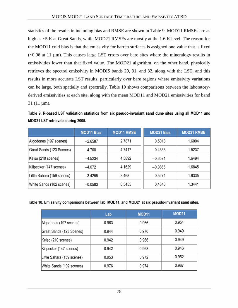
MODIS MOD21 LAND SURFACE TEMPERATURE AND EMISSIVITY ATBD
78
statistics of the results in including bias and RMSE are shown in Table 9. MOD11 RMSEs are as
high as ~5 K at Great Sands, while MOD21 RMSEs are mostly at the 1.6 K level. The reason for
the MOD11 cold bias is that the emissivity for barren surfaces is assigned one value that is fixed
(~0.96 at 11 µm). This causes large LST errors over bare sites where the mineralogy results in
emissivities lower than that fixed value. The MOD21 algorithm, on the other hand, physically
retrieves the spectral emissivity in MODIS bands 29, 31, and 32, along with the LST, and this
results in more accurate LST results, particularly over bare regions where emissivity variations
can be large, both spatially and spectrally. Table 10 shows comparisons between the laboratory-
derived emissivities at each site, along with the mean MOD11 and MOD21 emissivities for band
31 (11 µm).
Table 9. R-based LST validation statistics from six pseudo-invariant sand dune sites using all MOD11 and
MOD21 LST retrievals during 2005.
MOD11 Bias MOD11 RMSE
MOD21 Bias MOD21 RMSE
Algodones (197 scenes) 2.6587 2.7871 0.5018 1.6004
Great Sands (123 Scenes) 4.708 4.7417
0.4333 1.5237
Kelso (210 scenes) 4.5234 4.5892
0.6574 1.6494
Killpecker (147 scenes) 4.072 4.1629 0.0866 1.6845
Little Sahara (159 scenes) 3.4255 3.468 0.5274 1.6335
White Sands (102 scenes) 0.0583 0.5455 0.4843 1.3441
Table 10. Emissivity comparisons between lab, MOD11, and MOD21 at six pseudo-invariant sand sites.
Lab MOD11 MOD21
Algodones (197 scenes) 0.963 0.966 0.954
Great Sands (123 Scenes) 0.944 0.970 0.949
Kelso (210 scenes) 0.942 0.966 0.949
Killpecker (147 scenes) 0.942 0.968 0.946
Little Sahara (159 scenes) 0.953 0.972 0.952
White Sands (102 scenes) 0.976 0.974 0.967
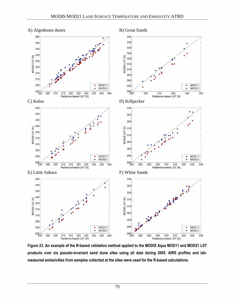
MODIS MOD21 LAND SURFACE TEMPERATURE AND EMISSIVITY ATBD
79
A) Algodones dunes
B) Great Sands
C) Kelso
D) Killpecker
E) Little Sahara
F) White Sands
Figure 23. An example of the R-based validation method applied to the MODIS Aqua MOD11 and MOD21 LST
products over six pseudo-invariant sand dune sites using all data during 2005. AIRS profiles and lab-
measured emissivities from samples collected at the sites were used for the R-based calculations.
MODIS MOD21 LAND SURFACE TEMPERATURE AND EMISSIVITY ATBD
80
11 References
Abdalati, W., & Steffen, K. (2001). Greenland ice sheet melt extent: 1979-1999. Journal of
Geophysical Research-Atmospheres, 106, 33983-33988
Anderson, M.C., Hain, C.R., Wardlow, B., Mecikalski, J.R., & Kustas, W.P. (2011a). Evaluation
of a drought index based on thermal remote sensing of evapotranspiration over the continental
U.S. Journal of Climate, 24, 2025-2044
Anderson, M.C., Kustas, W.P., Norman, J.M., Hain, C.R., Mecikalski, J.R., Schultz, L.,
Gonzalez-Dugo, M.P., Cammalleri, C., d'Urso, G., Pimstein, A., & Gao, F. (2011b). Mapping
daily evapotranspiration at field to continental scales using geostationary and polar orbiting
satellite imagery. Hydrology and Earth System Sciences, 15, 223-239
Augustine, J.A., DeLuisi, J.J., & Long, C.N. (2000). SURFRAD - A national surface radiation
budget network for atmospheric research. Bulletin of the American Meteorological Society, 81,
2341-2357
Baldridge, A.M., Hook, S.J., Grove, C.I., & Rivera, G. (2009). The ASTER Spectral Library
Version 2.0. Remote Sensing of Environment, 114, 711-715
Bannari, A., Omari, K., Teillet, R.A., & Fedosejevs, G. (2005). Potential of getis statistics to
characterize the radiometric uniformity and stability of test sites used for the calibration of earth
observation sensors. Ieee Transactions on Geoscience and Remote Sensing, 43, 2918-2926
Barducci, A., & Pippi, I. (1996). Temperature and emissivity retrieval from remotely sensed
images using the ''grey body emissivity'' method. Ieee Transactions on Geoscience and Remote
Sensing, 34, 681-695
Barnes, W.L., Pagano, T.S., & Salomonson, V.V. (1998). Prelaunch characteristics of the
Moderate Resolution Imaging Spectroradiometer (MODIS) on EOS-AM1. Ieee Transactions on
Geoscience and Remote Sensing, 36, 1088-1100
Barton, I.J., Zavody, A.M., Obrien, D.M., Cutten, D.R., Saunders, R.W., & Llewellyn-Jones,
D.T. (1989). Theoretical Algorithms for Satellite-Derived Sea-Surface Temperatures. Journal of
Geophysical Research-Atmospheres, 94, 3365-3375
Becker, F., & Li, Z.L. (1990). Temperature-Independent Spectral Indexes in Thermal Infrared
Bands. Remote Sensing of Environment, 32, 17-33
Benson, C.S. (1996). Stratigraphic studies in the snow and firn of the Greenland ice sheet, Snow,
Ice and Permafrost Research Establishment (now U.S. Army Cold Regions Research and
Engineering Laboratory). In
Berk, A. (1989). MODTRAN: A moderate resolution model for LOWTRAN 7. Spectral
Sciences, Inc., Burlington, MA.
Berk, A., Anderson, G.P., Acharya, P.K., Bernstein, L.S., Muratov, L., Lee, J., Fox, M., Adler-
Golden, S.M., Chetwynd, J.H., Hoke, M.L., Lockwood, R.B., Gardner, J.A., Cooley, T.W.,
Borel, C.C., & Lewis, P.E. (2005). MODTRANTM
5, A Reformulated Atmospheric Band Model
with Auxiliary Species and Practical Multiple Scattering Options: Update. In S.S. Sylvia & P.E.
Lewis (Eds.), Algorithms and Technologies for Multispectral, Hyperspectral, and Ultraspectral
Imagery XI. Bellingham, WA: Proceedings of SPIE
MODIS MOD21 LAND SURFACE TEMPERATURE AND EMISSIVITY ATBD
81
Bonan, G.B., Oleson, K.W., Vertenstein, M., Levis, S., Zeng, X.B., Dai, Y.J., Dickinson, R.E., &
Yang, Z.L. (2002). The land surface climatology of the community land model coupled to the
NCAR community climate model. Journal of Climate, 15, 3123-3149
Borbas, E., Knuteson, R., Seemann, S.W., Weisz, E., Moy, L., & Huang, H. (2007). A high
spectral resolution global land surface infrared emissivity database. In, Joint 2007 EUMETSAT
Meteorological Satellite &15th AMS Satellite Meteorology and Oceanography Conference.
Amsterdam, The Netherlands
Bosilovich, M.G., Chen, J.Y., Robertson, F.R., & Adler, R.F. (2008). Evaluation of global
precipitation in reanalyses. Journal of Applied Meteorology and Climatology, 47, 2279-2299
Brown, O., & Minnett, P. (1999). MODIS infrared sea surface temperature algorithm. Algorithm
Theoretical Basis Document Version 2, Univ. of Miami, Miami, Fla.
Coll, C., & Caselles, V. (1997). A split-window algorithm for land surface temperature from
advanced very high resolution radiometer data: Validation and algorithm comparison. Journal of
Geophysical Research-Atmospheres, 102, 16697-16713
Coll, C., Caselles, V., Galve, J.M., Valor, E., Niclos, R., Sanchez, J.M., & Rivas, R. (2005).
Ground measurements for the validation of land surface temperatures derived from AATSR and
MODIS data. Remote Sensing of Environment, 97, 288-300
Coll, C., Caselles, V., Valor, E., Niclos, R., Sanchez, J.M., Galve, J.M., & Mira, M. (2007).
Temperature and emissivity separation from ASTER data for low spectral contrast surfaces.
Remote Sensing of Environment, 110, 162-175
Coll, C., Wan, Z.M., & Galve, J.M. (2009a). Temperature-based and radiance-based validations
of the V5 MODIS land surface temperature product. Journal of Geophysical Research-
Atmospheres, 114, D20102, doi:20110.21029/22009JD012038
Coll, C., Wan, Z.M., & Galve, J.M. (2009b). Temperature-based and radiance-based validations
of the V5 MODIS land surface temperature product. Journal of Geophysical Research-
Atmospheres, 114, -
Comiso, J.C. (2006). Arctic warming signals from satellite observations. Weather, 61, 70-76
Cosnefroy, H.N., Leroy, M., & Briottet, X. (1996). Selection and characterization of Saharan and
Arabian desert sites for the calibration of optical satellite sensors. Remote Sensing of
Environment, 58, 101-114
de Vries, C., Danaher, T., Denham, R., Scarth, P., & Phinn, S. (2007). An operational
radiometric calibration procedure for the Landsat sensors based on pseudo-invariant target sites.
Remote Sensing of Environment, 107, 414-429
Deschamps, P.Y., & Phulpin, T. (1980). Atmospheric Correction of Infrared Measurements of
Sea-Surface Temperature Using Channels at 3.7, 11 and 12 Mu-M. Boundary-Layer
Meteorology, 18, 131-143
Francois, C., Brisson, A., Le Borgne, P., & Marsouin, A. (2002). Definition of a radiosounding
database for sea surface brightness temperature simulations - Application to sea surface
temperature retrieval algorithm determination. Remote Sensing of Environment, 81, 309-326
Francois, C., & Ottle, C. (1996). Atmospheric corrections in the thermal infrared: Global and
water vapor dependent Split-Window algorithms - Applications to ATSR and AVHRR data. Ieee
Transactions on Geoscience and Remote Sensing, 34, 457-470
MODIS MOD21 LAND SURFACE TEMPERATURE AND EMISSIVITY ATBD
82
French, A.N., Schmugge, T.J., Ritchie, J.C., Hsu, A., Jacob, F., & Ogawa, K. (2008). Detecting
land cover change at the Jornada Experimental Range, New Mexico with ASTER emissivities.
Remote Sensing of Environment, 112, 1730-1748
Galve, J.A., Coll, C., Caselles, V., & Valor, E. (2008). An atmospheric radiosounding database
for generating land surface temperature algorithms. IEEE Transactions on Geoscience and
Remote Sensing, 46, 1547-1557
Gillespie, A., Rokugawa, S., Hook, S., Matsunaga, T., & Kahle, A.B. (1999).
Temperature/Emissivity Separation Algorithm Theoretical Basis Document, Version 2.4,
ASTER TES ATBD, NASA Contract NAS5-31372, 31322 March, 31999
Gillespie, A., Rokugawa, S., Matsunaga, T., Cothern, J.S., Hook, S., & Kahle, A.B. (1998). A
temperature and emissivity separation algorithm for Advanced Spaceborne Thermal Emission
and Reflection Radiometer (ASTER) images. Ieee Transactions on Geoscience and Remote
Sensing, 36, 1113-1126
Gottsche, F.M., & Hulley, G.C. (2012). Validation of six satellite-retrieved land surface
emissivity products over two land cover types in a hyper-arid region. Remote Sensing of
Environment, 124, 149-158
Gustafson, W.T., Gillespie, A.R., & Yamada, G.J. (2006). Revisions to the ASTER
temperature/emissivity separation algorithm. In, 2nd International Symposium on Recent
Advances in Quantitative Remote Sensing. Torrent (Valencia), Spain
Hall, D.K., Williams Jr., R.S., Casey, K.A., Digirolamo, N.E., & Wan, Z. (2006). Satellite-
derived, melt-season surface temperature of the Greenland Ice Sheet (2000-2005) and its
relationship to mass balance. Geophysical Research Letters, 33:L11501,
doi:10.1029/2006GL026444
Hall, D.K., Williams, R.S., Luthcke, S.B., & Digirolamo, N.E. (2008). Greenland ice sheet
surface temperature, melt and mass loss: 2000-06. Journal of Glaciology, 54, 81-93
Hook, S.J., Dmochowski, J.E., Howard, K.A., Rowan, L.C., Karlstrom, K.E., & Stock, J.M.
(2005). Mapping variations in weight percent silica measured from multispectral thermal infrared
imagery - Examples from the Hiller Mountains, Nevada, USA and Tres Virgenes-La Reforma,
Baja California Sur, Mexico. Remote Sensing of Environment, 95, 273-289
Hook, S.J., Gabell, A.R., Green, A.A., & Kealy, P.S. (1992). A Comparison of Techniques for
Extracting Emissivity Information from Thermal Infrared Data for Geologic Studies. Remote
Sensing of Environment, 42, 123-135
Hook, S.J., Vaughan, R.G., Tonooka, H., & Schladow, S.G. (2007). Absolute radiometric in-
flight validation of mid infrared and thermal infrared data from ASTER and MODIS on the terra
spacecraft using the Lake Tahoe, CA/NV, USA, automated validation site. Ieee Transactions on
Geoscience and Remote Sensing, 45, 1798-1807
Hulley, G.C., & Hook, S.J. (2009a). Intercomparison of Versions 4, 4.1 and 5 of the MODIS
Land Surface Temperature and Emissivity Products and Validation with Laboratory
Measurements of Sand Samples from the Namib Desert, Namibia. Remote Sensing of
Environment, 113, 1313-1318
Hulley, G.C., & Hook, S.J. (2009b). The North American ASTER Land Surface Emissivity
Database (NAALSED) Version 2.0. Remote Sensing of Environment, 1967-1975
MODIS MOD21 LAND SURFACE TEMPERATURE AND EMISSIVITY ATBD
83
Hulley, G.C., & Hook, S.J. (2011). Generating Consistent Land Surface Temperature and
Emissivity Products Between ASTER and MODIS Data for Earth Science Research. Ieee
Transactions on Geoscience and Remote Sensing, 49, 1304-1315
Hulley, G.C., Hook, S.J., & Baldridge, A.M. (2008). ASTER land surface emissivity database of
California and Nevada. Geophysical Research Letters, 35, L13401, doi:
13410.11029/12008gl034507
Hulley, G.C., Hook, S.J., & Baldridge, A.M. (2009a). Validation of the North American ASTER
Land Surface Emissivity Database (NAALSED) Version 2.0 using Pseudo-Invariant Sand Dune
Sites. Remote Sensing of Environment, 113, 2224-2233
Hulley, G.C., Hook, S.J., & Baldridge, A.M. (2010). Investigating the Effects of Soil Moisture
on Thermal Infrared Land Surface Temperature and Emissivity Using Satellite Retrievals and
Laboratory Measurements. Remote Sensing of Environment, 114, 1480-1493
Hulley, G.C., Hook, S.J., Manning, E., Lee, S.Y., & Fetzer, E.J. (2009b). Validation of the
Atmospheric Infrared Sounder (AIRS) Version 5 (v5) Land Surface Emissivity Product over the
Namib and Kalahari Deserts. Journal of Geophysical Research Atmospheres, 114, D19104
Hulley, G.C., Hughes, T., & Hook, S.J. (2012). Quantifying Uncertainties in Land Surface
Temperature (LST) and Emissivity Retrievals from ASTER and MODIS Thermal Infrared Data.
Journal of Geophysical Research Atmospheres, in press.
Jimenez-Munoz, J.C., & Sobrino, J.A. (2010). A Single-Channel Algorithm for Land-Surface
Temperature Retrieval From ASTER Data. Ieee Geoscience and Remote Sensing Letters, 7, 176-
179
Jin, M.L., & Liang, S.L. (2006). An improved land surface emissivity parameter for land surface
models using global remote sensing observations. Journal of Climate, 19, 2867-2881
Justice, C., & Townshend, J. (2002). Special issue on the moderate resolution imaging
spectroradiometer (MODIS): a new generation of land surface monitoring. Remote Sensing of
Environment, 83, 1-2
Justice, C.O., Vermote, E., Townshend, J.R.G., Defries, R., Roy, D.P., Hall, D.K., Salomonson,
V.V., Privette, J.L., Riggs, G., Strahler, A., Lucht, W., Myneni, R.B., Knyazikhin, Y., Running,
S.W., Nemani, R.R., Wan, Z.M., Huete, A.R., van Leeuwen, W., Wolfe, R.E., Giglio, L., Muller,
J.P., Lewis, P., & Barnsley, M.J. (1998). The Moderate Resolution Imaging Spectroradiometer
(MODIS): Land remote sensing for global change research. Ieee Transactions on Geoscience
and Remote Sensing, 36, 1228-1249
Kalnay, E., Kanamitsu, M., & Baker, W.E. (1990). Global Numerical Weather Prediction at the
National-Meteorological-Center. Bulletin of the American Meteorological Society, 71, 1410-
1428
Kealy, M.J., Montgomery, M., & Dovidio, J.F. (1990). Reliability and Predictive-Validity of
Contingent Values - Does the Nature of the Good Matter. Journal of Environmental Economics
and Management, 19, 244-263
Kealy, P.S., & Hook, S. (1993). Separating temperature & emissivity in thermal infrared
multispectral scanner data: Implication for recovering land surface temperatures. Ieee
Transactions on Geoscience and Remote Sensing, 31, 1155-1164
MODIS MOD21 LAND SURFACE TEMPERATURE AND EMISSIVITY ATBD
84
Kinter, J.L., Shukla, J., Marx, L., & Schneider, E.K. (1988). A simulation of the winter and
summer circulations with the NMC global spectral model. Journal of Atmospheric Science, 45,
2486-2522
Kneizys, F.X., Abreu, L.W., Anderson, G.P., Chetwynd, J.H., Shettle, E.P., Berk, A., Bernstein,
L.S., Robertson, D.C., Acharya, P.K., Rothman, L.A., Selby, J.E.A., Gallery, W.O., & Clough,
S.A. (1996a). The MODTRAN 2/3 Report & LOWTRAN 7 Model, F19628-91-C-0132. In P.
Lab. (Ed.). Hanscom AFB, MA
Kneizys, F.X., Abreu, L.W., Anderson, G.P., Chetwynd, J.H., Shettle, E.P., Berk, A., Bernstein,
L.S., Robertson, D.C., Acharya, P.K., Rothman, L.A., Selby, J.E.A., Gallery, W.O., & Clough,
S.A. (1996b). The MODTRAN 2/3 Report & LOWTRAN 7 Model, F19628-91-C-0132. In,
Phillips Lab. Hanscom AFB, MA
Li, F.Q., Jackson, T.J., Kustas, W.P., Schmugge, T.J., French, A.N., Cosh, M.H., & Bindlish, R.
(2004). Deriving land surface temperature from Landsat 5 and 7 during SMEX02/SMACEX.
Remote Sensing of Environment, 92, 521-534
Li, Z.L., Becker, F., Stoll, M.P., & Wan, Z.M. (1999). Evaluation of six methods for extracting
relative emissivity spectra from thermal infrared images. Remote Sensing of Environment, 69,
197-214
Lyon, R. (1965). Analysis of ROcks by Spectral INfrared Emission (8 to 25 microns). Economic
Geology and the Bulletin of the Society of Economic Geologists, 60, 715-736
Masuda, K., Takashima, T., & Takayama, Y. (1988). Emissivity of Pure and Sea Waters for the
Model Sea-Surface in the Infrared Window Regions. Remote Sensing of Environment, 24, 313-
329
Matsunaga, T. (1994). A temperature-emissivity separation method using an empirical
relationship between the mean, the maximum, & the minimum of the thermal infrared
emissivity spectrum, in Japanese with English abstract. Journal Remote Sensing Society Japan,
14, 230-241
Mira, M., Valor, E., Boluda, R., Caselles, V., & Coll, C. (2007). Influence of soil water content
on the thermal infrared emissivity of bare soils: Implication for land surface temperature
determination. Journal of Geophysical Research-Earth Surface, 112, F04003
Mushkin, A., & Gillespie, A.R. (2005). Estimating sub-pixel surface roughness using remotely
sensed stereoscopic data. Remote Sensing of Environment, 99, 75-83
Norman, J.M., & Becker, F. (1995). Terminology in Thermal Infrared Remote-Sensing of
Natural Surfaces. Agricultural and Forest Meteorology, 77, 153-166
Ogawa, K. (2004). Mapping Surface Broadband Emissivity of the Sahara Desert Using ASTER
and MODIS Data. Earth Interactions, 8, -
Ogawa, K., Schmugge, T., Jacob, F., & French, A. (2003). Estimation of land surface window
(8-12 mu m) emissivity from multispectral thermal infrared remote sensing - A case study in a
part of Sahara Desert. Geophysical Research Letters, 30, -
Ogawa, K., Schmugge, T., & Rokugawa, S. (2006). Observations of the dependence of the
thermal infrared emissivity on soil moisture. Geophysical Research Abstracts, 8, 04996

MODIS MOD21 LAND SURFACE TEMPERATURE AND EMISSIVITY ATBD
85
Oleson, K.W., Bonan, G.B., Levis, S., & Vertenstein, M. (2004). Effects of land use change on
North American climate: impact of surface datasets and model biogeophysics. Climate
Dynamics, 23, 117-132
Palluconi, F., Hoover, G., Alley, R.E., Nilsen, M.J., & Thompson, T. (1999). An atmospheric
correction method for ASTER thermal radiometry over land, ASTER algorithm theoretical basis
document (ATBD), Revision 3, Jet Propulsion Laboratory, Pasadena, CA, 1999
Parkinson, C.L., Cavalieri, D.J., Gloersen, P., Zwally, H.J., & Comiso, J.C. (1999). Arctic sea ice
extents, areas, and trends, 1978-1996. Journal of Geophysical Research-Oceans, 104, 20837-
20856
Prata, A.J. (1994). Land-Surface Temperatures Derived from the Advanced Very High-
Resolution Radiometer and the Along-Track Scanning Radiometer .2. Experimental Results and
Validation of Avhrr Algorithms. Journal of Geophysical Research-Atmospheres, 99, 13025-
13058
Price, J.C. (1984). Land surface temperature measurements from the split window channels of
the NOAA 7 Advanced Very High Resolution Radiometer. Journal of Geophysical Research,
89, 7231-7237
Rhee, J., Im, J., & Carbone, G.J. (2010). Monitoring agricultural drought for arid and humid
regions using multi-sensor remote sensing data. Remote Sensing of Environment, 114, 2875-2887
Sabol, D.E., Gillespie, A.R., Abbott, E., & Yamada, G. (2009). Field validation of the ASTER
Temperature-Emissivity Separation algorithm. Remote Sensing of Environment, 113, 2328-2344
Salomonson, V.V., Barnes, W.L., Maymon, P.W., Montgomery, H.E., & Ostrow, H. (1989).
Modis - Advanced Facility Instrument for Studies of the Earth as a System. Ieee Transactions on
Geoscience and Remote Sensing, 27, 145-153
Seemann, S.W., Borbas, E., Li, J., Menzel, P., & Gumley, L.E. (2006). MODIS Atmospheric
Profile Retrieval Algorithm Theoretical Basis Document, Cooperative Institute for
Meteorological Satellite Studies, University of Wisconsin-Madison, Madison, WI, Version 6,
October 25, 2006
Seemann, S.W., Borbas, E.E., Knuteson, R.O., Stephenson, G.R., & Huang, H.L. (2008).
Development of a global infrared land surface emissivity database for application to clear sky
sounding retrievals from multispectral satellite radiance measurements. Journal of Applied
Meteorology and Climatology, 47, 108-123
Seemann, S.W., Li, J., Menzel, W.P., & Gumley, L.E. (2003). Operational retrieval of
atmospheric temperature, moisture, and ozone from MODIS infrared radiances. Journal of
Applied Meteorology, 42, 1072-1091
Snyder, W.C., Wan, Z., Zhang, Y., & Feng, Y.Z. (1998). Classification-based emissivity for land
surface temperature measurement from space. International Journal of Remote Sensing, 19,
2753-2774
Snyder, W.C., Wan, Z.M., Zhang, Y.L., & Feng, Y.Z. (1997). Thermal infrared (3-14 mu m)
bidirectional reflectance measurements of sands and soils. Remote Sensing of Environment, 60,
101-109
Strahler, A.H., Zhang, X., Cooper, A., Schaaf, C., Friedl, M., Hodges, J., Baccini, A., & Gao, F.
(2002). Validation of the consistent-year v003 MODIS land cover product. http://www-
modis.bu.edu/landcover/userguidelc/consistent.htm

MODIS MOD21 LAND SURFACE TEMPERATURE AND EMISSIVITY ATBD
86
Susskind, J., Barnet, C.D., & Blaisdell, J.M. (2003). Retrieval of atmospheric and surface
parameters from AIRS/AMSU/HSB data in the presence of clouds. Ieee Transactions on
Geoscience and Remote Sensing, 41, 390-409
Teillet, P.M., Fedosejevs, G., Gautier, R.P., & Schowengerdt, R.A. (1998). Uniformity
characterization of land test sites used for radiometric calibration of earth observation sensors.
In, Proc. 20th Can. Symp. Remote Sensing (pp. 1-4). Calgary, AB, Canada
Tobin, D.C., Revercomb, H.E., Knuteson, R.O., Lesht, B.M., Strow, L.L., Hannon, S.E., Feltz,
W.F., Moy, L.A., Fetzer, E.J., & Cress, T.S. (2006). Atmospheric Radiation Measurement site
atmospheric state best estimates for Atmospheric Infrared Sounder temperature and water vapor
retrieval validation. Journal of Geophysical Research-Atmospheres, 111, -
Tonooka, H. (2001). An atmospheric correction algorithm for thermal infrared multispectral data
over land - A water-vapor scaling method. Ieee Transactions on Geoscience and Remote
Sensing, 39, 682-692
Tonooka, H. (2005). Accurate atmospheric correction of ASTER thermal infrared imagery using
the WVS method. Ieee Transactions on Geoscience and Remote Sensing, 43, 2778-2792
Tonooka, H., & Palluconi, F.D. (2005). Validation of ASTER/TIR standard atmospheric
correction using water surfaces. Ieee Transactions on Geoscience and Remote Sensing, 43, 2769-
2777
Tonooka, H., Palluconi, F.D., Hook, S.J., & Matsunaga, T. (2005). Vicarious calibration of
ASTER thermal infrared bands. Ieee Transactions on Geoscience and Remote Sensing, 43, 2733-
2746
Vaughan, R.G., Hook, S.J., Calvin, W.M., & Taranik, J.V. (2005). Surface mineral mapping at
Steamboat Springs, Nevada, USA, with multi-wavelength thermal infrared images. Remote
Sensing of Environment, 99, 140-158
Wan, Z. (1999). MODIS Land-Surface Temperature Algorithm Theoretical Basis Document
(LST ATBD), Version 3.3, University of California, Santa Barbara, April 1999
Wan, Z., & Li, Z.L. (2008). Radiance-based validation of the V5 MODIS land-surface
temperature product. International Journal of Remote Sensing, 29, 5373-5395
Wan, Z., Zhang, Y., Zhang, Q., & Li, Z.L. (2004). Quality assessment and validation of the
MODIS global land surface temperature. International Journal of Remote Sensing, 25, 261-274
Wan, Z.M. (2008). New refinements and validation of the MODIS Land-Surface
Temperature/Emissivity products. Remote Sensing of Environment, 112, 59-74
Wan, Z.M., & Dozier, J. (1996). A generalized split-window algorithm for retrieving land-
surface temperature from space. Ieee Transactions on Geoscience and Remote Sensing, 34, 892-
905
Wan, Z.M., & Li, Z.L. (1997). A physics-based algorithm for retrieving land-surface emissivity
and temperature from EOS/MODIS data. Ieee Transactions on Geoscience and Remote Sensing,
35, 980-996
Wang, K.C., & Liang, S.L. (2009). Evaluation of ASTER and MODIS land surface temperature
and emissivity products using long-term surface longwave radiation observations at SURFRAD
sites. Remote Sensing of Environment, 113, 1556-1565
MODIS MOD21 LAND SURFACE TEMPERATURE AND EMISSIVITY ATBD
87
Watson, K. (1992). Spectral Ratio Method for Measuring Emissivity. Remote Sensing of
Environment, 42, 113-116
Watson, K., Kruse, F.A., & Hummermiller, S. (1990). Thermal Infrared Exploration in the Carlin
Trend, Northern Nevada. Geophysics, 55, 70-79
Yao, Z.G., Li, J., Li, J.L., & Zhang, H. (2011). Surface Emissivity Impact on Temperature and
Moisture Soundings from Hyperspectral Infrared Radiance Measurements. Journal of Applied
Meteorology and Climatology, 50, 1225-1235
Yu, Y., Pinheiro, J.L., & Privette, J.L. (2006). Correcting Land Surface Temperature
Measurements for Directional Emissivity Over 3-D Structured Vegetation. Proc. SPIE, 6298,
629817, DOI:629810.621117/629812.682951
Yu, Y., Privette, J.L., & Pinheiro, A.C. (2008). Evaluation of split-window land surface
temperature algorithms for generating climate data records. IEEE Transactions on Geoscience
and Remote Sensing, 46, 179-192
Yu, Y.Y., Privette, J.L., & Pinheiro, A.C. (2005). Analysis of the NPOESS VIIRS land surface
temperature algorithm using MODIS data. Ieee Transactions on Geoscience and Remote
Sensing, 43, 2340-2350
Zeng, Q.C., Zhang, X.H., Liang, X.Z., Yuan, C.G., & Chen, S.F. (1989). Documentation of IAP
two-level atmospheric general circulation model. In U.S.D.o. Energy (Ed.) (p. 383 pp.).
Washington, D.C.
Zhou, L., Dickinson, R.E., Ogawa, K., Tian, Y., Jin, M., Schmugge, T., & Tsvetsinskaya, E.
(2003a). Relations between albedos and emissivities from MODIS and ASTER data over North
African desert. Geophysical Research Letters, 30, -
Zhou, L., Dickinson, R.E., Tian, Y., Jin, M., Ogawa, K., Yu, H., & Schmugge, T. (2003b). A
sensitivity study of climate and energy balance simulations with use of satellite-derived
emissivity data over Northern Africa and the Arabian Peninsula. Journal of Geophysical
Research-Atmospheres, 108, 4795