lab 6 digital data and basic table operations in arcmap€¦ · lab 6: digital data and basic table...
TRANSCRIPT

GIS Fundamentals: Digital Data, Basic Tables Lab 6
1
Lab 6: Digital Data and Basic Table Operations in ArcMap
What You’ll Learn: This lab introduces some commonly available digital data sets, and introduces other digital data. Data: Unless noted, data are in UTM Zone 15, NAD83, meters, coordinates, and the
data files are found in the \L6 subdirectory, including: US_cities, a point layers of cities and towns, in NAD83 geographic coordinates, cen_Stx_U83, a subset of U.S. census bureau block group data, for a small area
spanning the Minnesota/Wisconsin border, County_2010Census_DP1.zip, a compressed file of county census data for the U.S., in
a .zip format, USGS_sheds, watershed boundaries at the hydrologic unit code level 8 (HUC-8), NED_lstx30, a National Elevation Dataset for the lower St. Croix HUC-8 watershed NHD_LStx_high.mdb, a National Hydrologic Dataset geodatabase for the lower St.
Croix HUC-8 watershed, Stil_wetU83, wetlands data for the Stillwater, Minnesota USGS 7.5 minute quadrangle, Citiesx010g.shp, a point shapefile layer, NAD83(86) geographic coordinates, in case
you have trouble downloading the original from a national website. What You’ll Produce: five maps: 1) a Kodiak Island map using online and downloaded data, 2) a population density map from a census data set, with subset cities from a US data set, 3) a proportional symbol map of county population for the lower 48 U.S. states, 4) a shaded relief/hydrography map, and 5) a map of wetlands by size class. Background: Much data is available for download from the worldwide web, as described in Chapter 7 and appendix B of the GIS Fundamentals textbook. This exercise introduces digital data downloads with a few examples, basic selection by locations, and basic table operations. Most GIS store attribute data in tables. Each feature in a data layers is associated with a row in a table. We can select data manually from the geographic features, or via the tables. We also often add or remove table columns, and calculate values into columns. You’ll be doing this sort of table manipulation in most of the remaining labs, so we’ll keep these first selections and subsequent operations rather simple. We’ll manipulate data and compose maps that contain some of the wide range of data that are available for download from web sources.
GIS Fundamentals: Digital Data, Basic Tables Lab 6
2
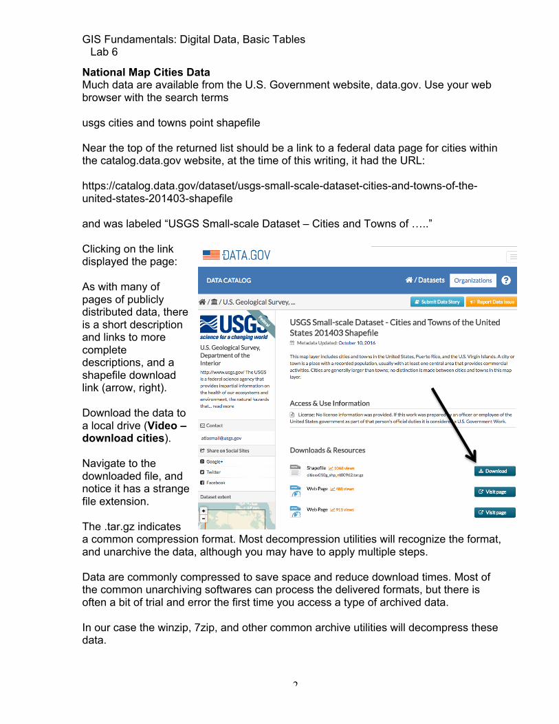
National Map Cities Data Much data are available from the U.S. Government website, data.gov. Use your web browser with the search terms usgs cities and towns point shapefile Near the top of the returned list should be a link to a federal data page for cities within the catalog.data.gov website, at the time of this writing, it had the URL: https://catalog.data.gov/dataset/usgs-small-scale-dataset-cities-and-towns-of-the-united-states-201403-shapefile and was labeled “USGS Small-scale Dataset – Cities and Towns of …..” Clicking on the link displayed the page: As with many of pages of publicly distributed data, there is a short description and links to more complete descriptions, and a shapefile download link (arrow, right). Download the data to a local drive (Video – download cities). Navigate to the downloaded file, and notice it has a strange file extension. The .tar.gz indicates a common compression format. Most decompression utilities will recognize the format, and unarchive the data, although you may have to apply multiple steps. Data are commonly compressed to save space and reduce download times. Most of the common unarchiving softwares can process the delivered formats, but there is often a bit of trial and error the first time you access a type of archived data. In our case the winzip, 7zip, and other common archive utilities will decompress these data.

GIS Fundamentals: Digital Data, Basic Tables Lab 6
3
You should download and decompress your own data sets for practice. If you are unable to, we’ve provided an unarchived version in the data set, in the folder citiesx010g_shp. Once the data are downloaded and decompressed, start ArcMap and add the cities point shapefile. It should look something like the figure to the right. The metadata states these are in geographic coordinates. The data set includes cities in Alaska that are east and west of the international data line, so some get wrapped to the right side of the map. We’re interested in Kodiak Island in south-central Alaska, so zoom to the area indicated by the arrow at right. Let’s add a basemap. This is a very common source of basic data if you only wish to use them for display. Click on the Add Data button, then select Add Basemap (figure at right). Select the Topographic tile from the options provided, usually near the left center of the choices. Your display should approximate that shown to the right, with a topographic map underlaying the cities. Manual Selection We want to select and save only a subset of cities displayed. Zoom to display Kodiak Island, shown by the arrow at right. Change the data frame projection to Alaska State Plane NAD 1983

GIS Fundamentals: Digital Data, Basic Tables Lab 6
4
(2011) State Plane zone Alaska 5 (FIPS 5005), US feet. Remember that the data frame coordinate system specification is found by:
• a right click the data frame name (Layers), then • Properties - Coordinate System tab • Projected Coordinates – State Plane – NAD1983 (2011) (US Feet) • Then selecting the appropriate zone.
Ignore the warnings about coordinate system incompatibility, Arc is upset about different flavors of the NAD83 datums, but our data here are coarse resolution (why does that mean we can ignore datum differences?). Now your data frame should approximate the figure at left, without the vertical compression near the poles when we display geographic coordinate data. We wish to select the cities on Kodiak Island (Video: Manual Feature Select). Activate the select feature cursor (see figure below right). If you click and hold on the Select Feature tool, it will show various options for manually selection. For most of these, you click and hold-drag to define a selection region, or click multiple times to form a boundary. Click on the Select by Lasso tool.

GIS Fundamentals: Digital Data, Basic Tables Lab 6
5
Position the cursor near the island edge, left click and hold the left mouse button, and draw a polygon that includes all the cities on Kodiak Island; then release the mouse button. This should show a polygon as you’re drawing (see at right), and On completing the polygon, release the mouse button to select the subset of cities. Only the those inside the polygon should be colored cyan (not shown).
Save the selected features by • right clicking on the
citiesx010g in the Table of contents, then
• Data – Export Data • specify an output for only
the selected features, here I saved to a shapefile named KodiakCities.
Remove the original, large data set from the data frame. Selection greatly reduces the data set size, eases use, and the speed of redraws. Label the cities in the view (right click on the data set, then Properties, the Label tab, and then check on and set options):
GIS Fundamentals: Digital Data, Basic Tables Lab 6
6
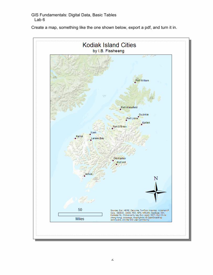
Create a map, something like the one shown below, export a pdf, and turn it in.

GIS Fundamentals: Digital Data, Basic Tables Lab 6
7
Census Data - 1 Add a new data frame or a new project. Add the census data, cen_StX_U83.shp to your new empty data frame. This is a subset of the census attributes for a portion of the Minnesota/Wisconsin border. Each polygon is a block group, a unit of aggregation for population census data. Open the attribute table (right click on cen_StX_U83 in TOC, then click Open Attribute Table), and inspect the values for the column labeled pden_psqkm. This is the population density for the census block groups in this area. Next, right click on the column name, and select Statistics (see right). This should display a column summary, and a histogram (see below).
Note that the data has quite a few small values, and a few very large values. This “long-tailed” distribution is common in some types of data, and often displays better with a non-uniform spacing of symbol ranges. We’ll demonstrate. Close the table, and open the Symbology Properties menu for the census data layer. Symbolize this as Quantities-Graduated Colors, and display the population density data (pden_psqkm) in the Value field, with no normalization. Keep the default number of classes, and select a gradient color ramp (in the example
GIS Fundamentals: Digital Data, Basic Tables Lab 6
8
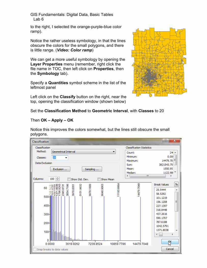
to the right, I selected the orange-purple-blue color ramp). Notice the rather useless symbology, in that the lines obscure the colors for the small polygons, and there is little range. (Video: Color ramp) We can get a more useful symbology by opening the Layer Properties menu (remember, right click the file name in TOC, then left click on Properties, then the Symbology tab). Specify a Quantities symbol scheme in the list of the leftmost panel Left click on the Classify button on the right, near the top, opening the classification window (shown below) Set the Classification Method to Geometric Interval, with Classes to 20 Then OK – Apply – OK Notice this improves the colors somewhat, but the lines still obscure the small polygons.

GIS Fundamentals: Digital Data, Basic Tables Lab 6
9
To remove the lines, open the Layer Properties menu one more time. Now, left click in the first color patch and select all the categories then select Properties for Selected Symbols(s). This should open the Symbol Selector menu. Set the Outline Color to “No Color”. Then left click on OK – Apply – OK

GIS Fundamentals: Digital Data, Basic Tables Lab 6
10
This should display the layer in a manner similar to that shown below. This symbology provides a clearer view of the variation in the data, due both to removal of the border lines, and placing a geometric spacing of symbol ranges. Note that there are many other options that appear in the menu that contains the Properties for All Symbols. You may group, flip, ramp, or otherwise change a set of selected symbols, or all symbols. Experiment with these to see their effects. Selection by Location Add the US_cities.shp point layer to the data frame. These are data on cities for the entire U.S. and territories. Use the Zoom to Full
Extent button to view the entire dataset, and then Zoom to Previous Extent button to return to the area of the cen_StX_U83.shp area. It is burdensome to work with a large data set when we only wish a small portion or subset. Select just the cities data that corresponding with our census data set. (Videos: 1) Select by a Layer; and 2) More Symbols) Do this by: Selection > Select by Location in the main menu
GIS Fundamentals: Digital Data, Basic Tables Lab 6
11
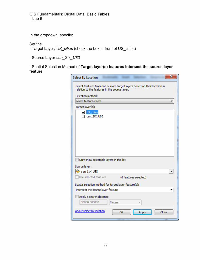
In the dropdown, specify: Set the - Target Layer, US_cities (check the box in front of US_cities) - Source Layer cen_Stx_U83 - Spatial Selection Method of Target layer(s) features intersect the source layer feature.

GIS Fundamentals: Digital Data, Basic Tables Lab 6
12
Then Apply – OK. This should display a view similar to the right. The selected cities show up in the current selection color, in this case, cyan. Saving a Selected Set to a New File To save this selected set into a new file: Right click on the US_cities file name in the Table of Contents, Left click on Data > Export. Make sure you specify “Export: Selected features”
GIS Fundamentals: Digital Data, Basic Tables Lab 6
13
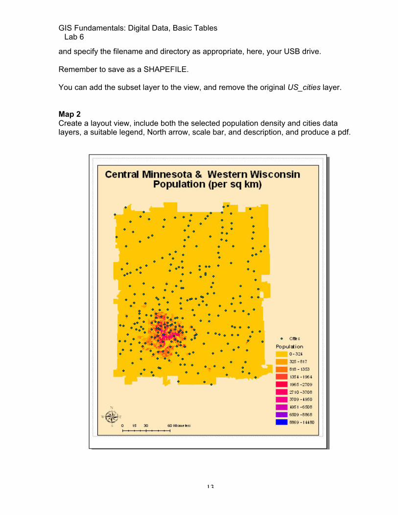
and specify the filename and directory as appropriate, here, your USB drive. Remember to save as a SHAPEFILE. You can add the subset layer to the view, and remove the original US_cities layer. Map 2 Create a layout view, include both the selected population density and cities data layers, a suitable legend, North arrow, scale bar, and description, and produce a pdf.

GIS Fundamentals: Digital Data, Basic Tables Lab 6
14
Census Data - 2 This is to practice what you’ve already learned in this and previous labs, without much specific instruction, and to teach you a tool that helps winnow columns, something often done after downloading data. Decompress the file County_2010Census_DP1 file in the data directory. It contains summary population data for all counties in the U.S. and territories, and was downloaded from the site: https://www.census.gov/geo/maps-data/data/tiger-data.html Note that there is a set of shapefiles, and an Excel file describing the variables in the shapefiles. You often get ancillary files, often text, sometimes other formats, that describe downloaded spatial data. Open the Excel file. Notice that there are tens of variable (columns) in the table. If we’re not interested in all of them, they take up space, reduce performance, and clutter our view. This often happens, so we need to subset the table. We’re primarily interested in total population. Verify in the Excel file that this variable is in the column labeled DP0010001. We also want to keep the FID, Shape, Geoid10, and NAMELSAD10 variables. Create a new project or data frame, and add the shapefile to the frame. Notice that there are data for all the U.S., including Alaska, Hawaii, and Puerto Rico. We wish to save the data for only the lower 48 U.S. states. Subset the data using the manual selection methods learned above, leaving out Alaska, Hawaii, Puerto Rico, and other outlying territories. Save the lower 48 states to a new file named something like Lower48. Add the Lower48 layer to your data frame, and remove the original County_2010Census_DP1 layer. Open the table and inspect the columns. Notice there are many, most starting with a DP and then various strings of numbers. It would be helpful to delete most of the columns, keeping only FID, shape, GEOID, NAMELSAD10, and DP0010001. (Video: Field Delete)

GIS Fundamentals: Digital Data, Basic Tables Lab 6
15
We can delete a single column by right clicking on the column name, and then clicking on Delete Field in the dropdown menu. This would get rather tedious for the tens of extra fields in this table; we’d like a batch delete tool. We can delete several columns at once with the Delete Field command. It isn’t on any toolbar, but we’ll show you how to search for tools, including those on toolbars that you know exist, and remember a fragment of their name, but have trouble finding. Open the Search for Tools utility, found under the Geoprocessing label along the top of the main ArcMap window:
GIS Fundamentals: Digital Data, Basic Tables Lab 6
16
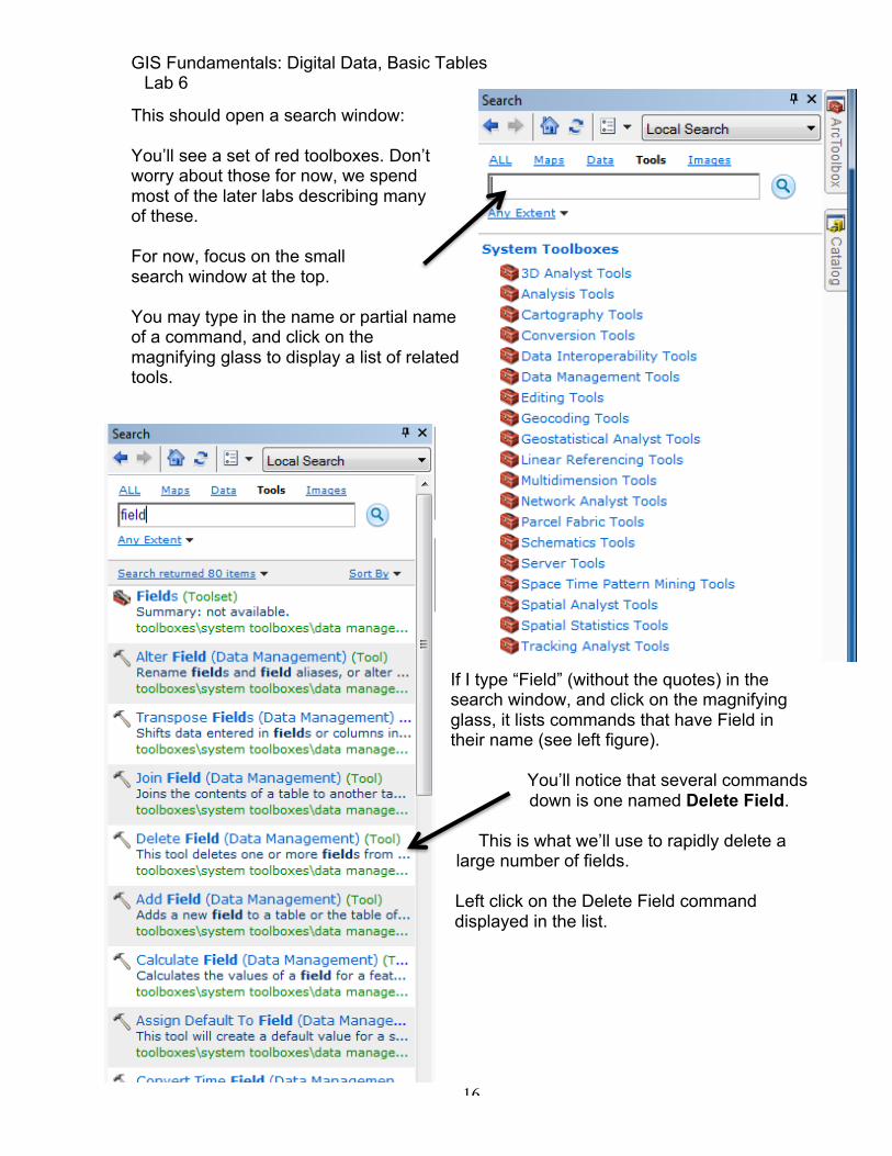
This should open a search window: You’ll see a set of red toolboxes. Don’t worry about those for now, we spend most of the later labs describing many of these. For now, focus on the small search window at the top. You may type in the name or partial name of a command, and click on the magnifying glass to display a list of related tools.
If I type “Field” (without the quotes) in the search window, and click on the magnifying glass, it lists commands that have Field in their name (see left figure).
You’ll notice that several commands down is one named Delete Field.
This is what we’ll use to rapidly delete a
large number of fields. Left click on the Delete Field command displayed in the list.
GIS Fundamentals: Digital Data, Basic Tables Lab 6
17
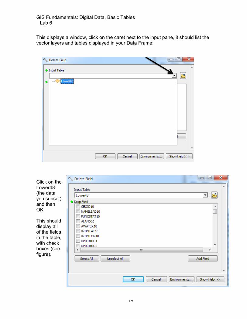
This displays a window, click on the caret next to the input pane, it should list the vector layers and tables displayed in your Data Frame:
Click on the Lower48 (the data you subset), and then OK This should display all of the fields in the table, with check boxes (see figure).

GIS Fundamentals: Digital Data, Basic Tables Lab 6
18
We check the boxes next to fields we wish to delete, then on hitting o.k., they are removed from the table. We wish to keep the GEOID, NAMELSAD10, and DP0010001. We don’t have the ability to delete the FID and Shape items, as these are key for maintaining the table, and not in the list. It is perhaps easiest to click on the Select All button, and then uncheck the few items we want to keep. However you do it, check variables to delete the un-needed columns, then click OK to remove the unwanted items. Once the tool completes, open the table and verify it worked as expected:
GIS Fundamentals: Digital Data, Basic Tables Lab 6
19
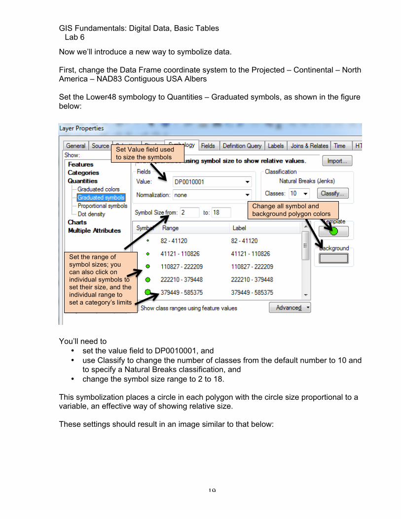
Now we’ll introduce a new way to symbolize data. First, change the Data Frame coordinate system to the Projected – Continental – North America – NAD83 Contiguous USA Albers Set the Lower48 symbology to Quantities – Graduated symbols, as shown in the figure below:
You’ll need to
• set the value field to DP0010001, and • use Classify to change the number of classes from the default number to 10 and
to specify a Natural Breaks classification, and • change the symbol size range to 2 to 18.
This symbolization places a circle in each polygon with the circle size proportional to a variable, an effective way of showing relative size. These settings should result in an image similar to that below:
Change all symbol and background polygon colors
Set Value field used to size the symbols
Set the range of symbol sizes; you can also click on individual symbols to set their size, and the individual range to set a category’s limits
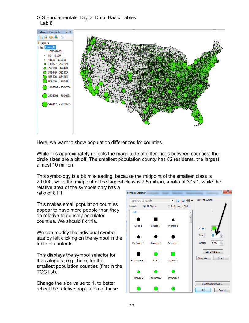
GIS Fundamentals: Digital Data, Basic Tables Lab 6
20
Here, we want to show population differences for counties. While this approximately reflects the magnitude of differences between counties, the circle sizes are a bit off. The smallest population county has 82 residents, the largest almost 10 million. This symbology is a bit mis-leading, because the midpoint of the smallest class is 20,000, while the midpoint of the largest class is 7.5 million, a ratio of 375:1, while the relative area of the symbols only has a ratio of 81:1. This makes small population counties appear to have more people than they do relative to densely populated counties. We should fix this. We can modify the individual symbol size by left clicking on the symbol in the table of contents. This displays the symbol selector for the category, e.g., here, for the smallest population counties (first in the TOC list): Change the size value to 1, to better reflect the relative population of these
GIS Fundamentals: Digital Data, Basic Tables Lab 6
21
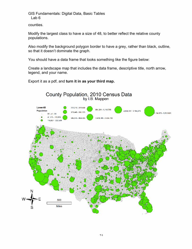
counties. Modify the largest class to have a size of 48, to better reflect the relative county populations. Also modify the background polygon border to have a grey, rather than black, outline, so that it doesn’t dominate the graph. You should have a data frame that looks something like the figure below: Create a landscape map that includes the data frame, descriptive title, north arrow, legend, and your name. Export it as a pdf, and turn it in as your third map.

GIS Fundamentals: Digital Data, Basic Tables Lab 6
22
Digital Elevation and NHD Data We’ll now explore digital elevation and related hydrologic data a bit. We’ll hold off an in-depth treatment of DEMs until Chapter 11 in the GIS Fundamentals textbook, and a later lesson. We’ll just introduce the data, and you show how to make an interesting shaded-relief map, suitable for backgrounds and many illustrations. Create a new ArcMap project, and set the data frame coordinate system to the UTM Zone 15N, NAD83 projection. Add the USGS_sheds.shp dataset to the data frame. These are watershed boundaries derived from elevation data, and downloaded from the US Geological Survey. Label these features: Right click on USGS_sheds in the TOC > Properties > Labels Then left click on the checkbox “label features in this layer”, Choose SUBBASIN as the Label Field, and then Apply - OK This should place the name of the each sub-basin within a polygon, something like the figure to the right. Try to copy/create a data set that consists of the outline of only the Lower St. Croix watershed, near the center of the data set. (See selection tips on Website document Summary Overheads for lab exercise page 13) We won’t give you exact instructions, we’ve covered it before, but here is a hint. Use a selection tool (there are several selection methods/tools that will work), then Data > Export to save your data to a new file shapefile. Now, remove all the data from your data frame. Create a Shaded-relief Elevation Map (Video: Shaded Relief) Add the ned_lstx30 DEM to your data frame. Use Properties > Symbology to display the Layer Properties menu and set a stretched color ramp. Use a Stretch Type of Standard Deviations, set n: 2, and use the elevation color ramp:

GIS Fundamentals: Digital Data, Basic Tables Lab 6
23
Select Apply, Okay. Now, calculate a hillshade surface: Select ArcToolbox à Spatial Analysisà Surfaceà Hillshade.

GIS Fundamentals: Digital Data, Basic Tables Lab 6
24
This should open a Hillshade menu.
Set the Input raster to ned_lstx30 (the DEM). Select a location for the output and a name, Hillshade1 for example. Keep the Azimuth at 315 (direction to the Sun). Set the Altitude to 25 (Sun’s elevation). Check the box to Model shadows. Set the Z factor to 4 (4x vertical exaggeration), then OK. This should create a hillshade surface, and if it isn’t done automatically, place it on top of your DEM. Now make the hillshade semi-transparent: Right click on the hillshade in the TOC, then Properties > Display. Set the Transparency to something near 50%, then Apply – OK. You should now see the DEM, with the hillshading “painted” on top (see the figure, below, shown with additional data added). This is a commonly-used affect in producing
GIS Fundamentals: Digital Data, Basic Tables Lab 6
25
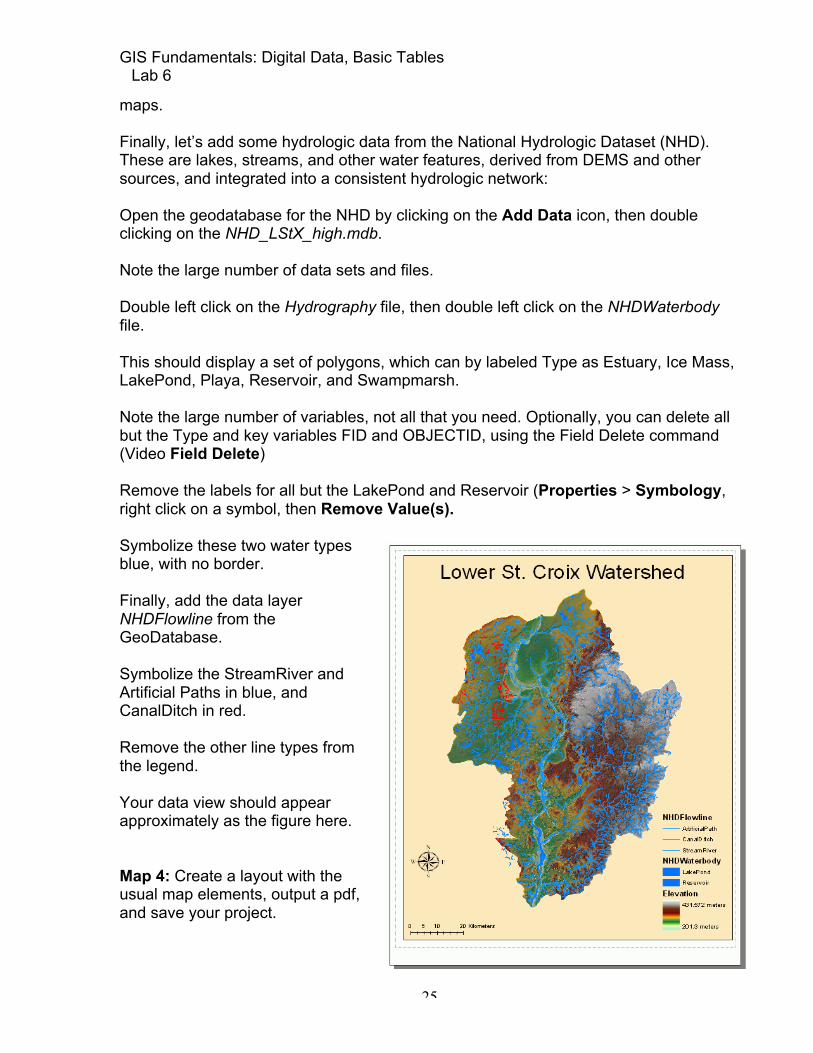
maps. Finally, let’s add some hydrologic data from the National Hydrologic Dataset (NHD). These are lakes, streams, and other water features, derived from DEMS and other sources, and integrated into a consistent hydrologic network: Open the geodatabase for the NHD by clicking on the Add Data icon, then double clicking on the NHD_LStX_high.mdb. Note the large number of data sets and files. Double left click on the Hydrography file, then double left click on the NHDWaterbody file. This should display a set of polygons, which can by labeled Type as Estuary, Ice Mass, LakePond, Playa, Reservoir, and Swampmarsh. Note the large number of variables, not all that you need. Optionally, you can delete all but the Type and key variables FID and OBJECTID, using the Field Delete command (Video Field Delete) Remove the labels for all but the LakePond and Reservoir (Properties > Symbology, right click on a symbol, then Remove Value(s). Symbolize these two water types blue, with no border. Finally, add the data layer NHDFlowline from the GeoDatabase. Symbolize the StreamRiver and Artificial Paths in blue, and CanalDitch in red. Remove the other line types from the legend. Your data view should appear approximately as the figure here. Map 4: Create a layout with the usual map elements, output a pdf, and save your project.

GIS Fundamentals: Digital Data, Basic Tables Lab 6
26
NWI Data and Basic Table Manipulations Open a new ArcMap project, and Add the data layer Stil_wetU83.shp to a new, empty project. (Video: Manual Selection in Tables) Right click on the Stil_wetU83 layer in the table of contents, then left click on Open Attribute Table in the dropdown menu. You will see the attributes of the wetlands layer. The Field called “Area” displays the area of the polygon in square meters (m2). The “Wet_type” field displays the type of wetland. Detail codes are listed at the end of this document. Right click over the heading of the “Area” column and select Sort Descending (as shown right). This brings the largest polygons to the top of the table. Notice that the largest areas are coded “U”, for uplands, and “Out”, area outside the mapping jurisdiction for these data, in this case, in Wisconsin. We will add a new variable, and manually classify the polygons by their size, which is contained in the “Area” attribute. Left click on the Table Options

GIS Fundamentals: Digital Data, Basic Tables Lab 6
27
and select “Add Field”. This will add a new empty field (column) to you file. Name the field “Size”, select the Type as “Text” and change the Length to 10 (as shown at right). Left click on Okay.
GIS Fundamentals: Digital Data, Basic Tables Lab 6
28
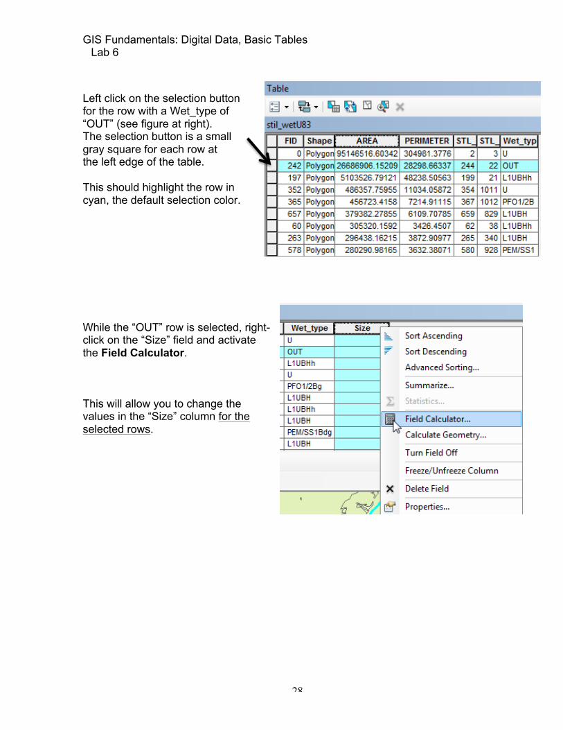
Left click on the selection button for the row with a Wet_type of “OUT” (see figure at right). The selection button is a small gray square for each row at the left edge of the table. This should highlight the row in cyan, the default selection color. While the “OUT” row is selected, right-click on the “Size” field and activate the Field Calculator. This will allow you to change the values in the “Size” column for the selected rows.
GIS Fundamentals: Digital Data, Basic Tables Lab 6
29
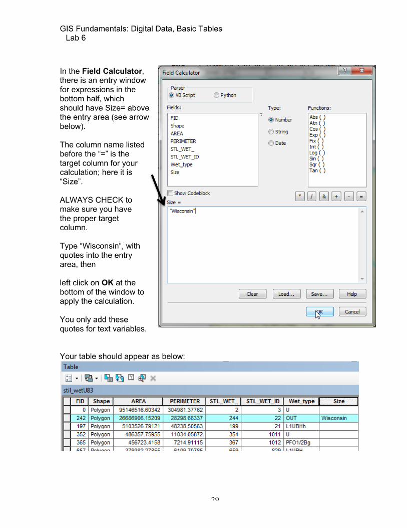
In the Field Calculator, there is an entry window for expressions in the bottom half, which should have Size= above the entry area (see arrow below). The column name listed before the “=” is the target column for your calculation; here it is “Size”. ALWAYS CHECK to make sure you have the proper target column. Type “Wisconsin”, with quotes into the entry area, then left click on OK at the bottom of the window to apply the calculation. You only add these quotes for text variables. Your table should appear as below:

GIS Fundamentals: Digital Data, Basic Tables Lab 6
30
Now sort the field in descending order by Wet_type. It should appear as the figure, with all the U Wet_types listed at the top: Left click on the selection button for the first row with a U (for Upland) Wet_type. It should show colored in cyan. Hold down the keyboard shift key, and left-click on the LAST row with a U in Wet_type. This should select all the upland polygons in the data set (see figure at right). Use the Field Calculator as before to assign JUST THESE SELECTED UPLAND polygons with a value of “Upland” in the size column. After you apply the calculation, review the columns to ensure that you applied it correctly, and that all the U Wet_types are correctly listed as Upland in the size field (not shown in our figures here). Now we wish to do a similar kind of manual selection and assignment, recording it in the size column, to create three
GIS Fundamentals: Digital Data, Basic Tables Lab 6
31
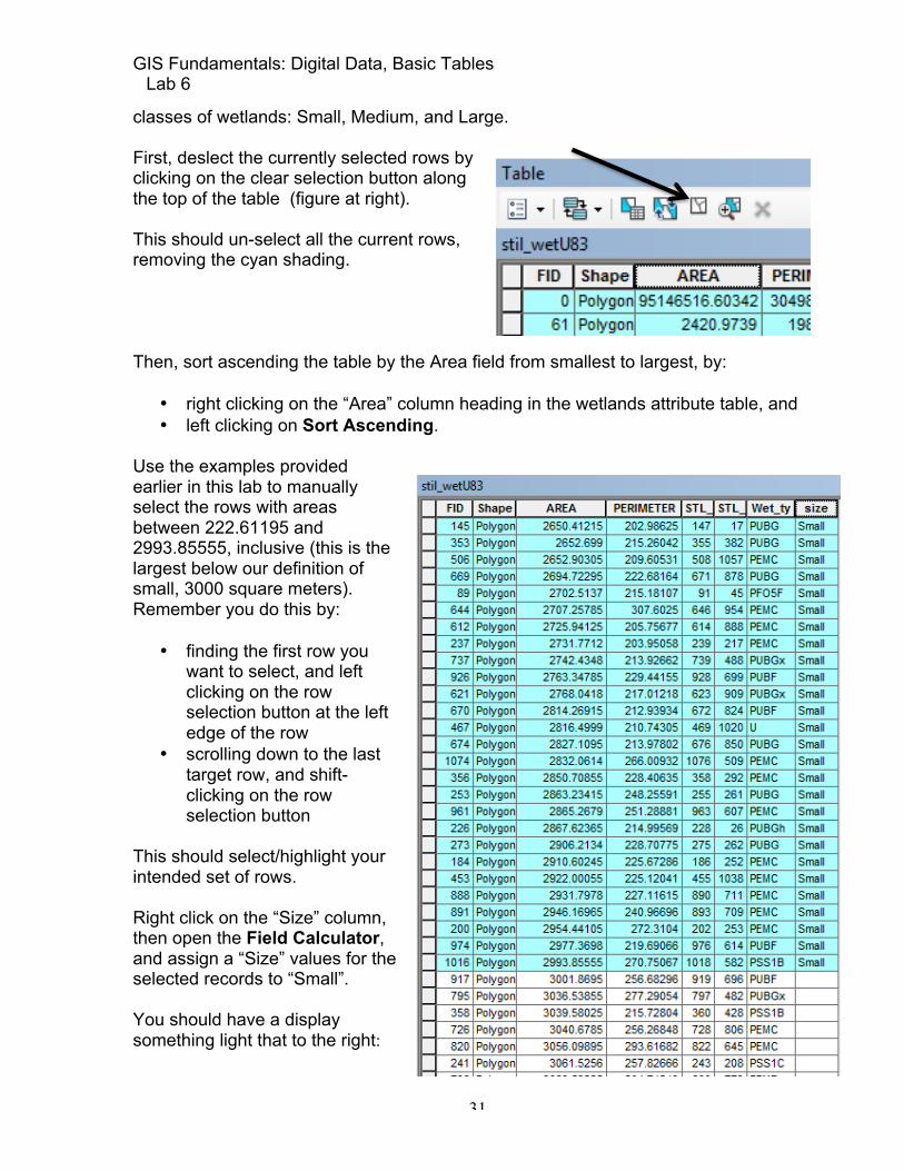
classes of wetlands: Small, Medium, and Large. First, deslect the currently selected rows by clicking on the clear selection button along the top of the table (figure at right). This should un-select all the current rows, removing the cyan shading. Then, sort ascending the table by the Area field from smallest to largest, by:
• right clicking on the “Area” column heading in the wetlands attribute table, and • left clicking on Sort Ascending.
Use the examples provided earlier in this lab to manually select the rows with areas between 222.61195 and 2993.85555, inclusive (this is the largest below our definition of small, 3000 square meters). Remember you do this by:
• finding the first row you want to select, and left clicking on the row selection button at the left edge of the row
• scrolling down to the last target row, and shift-clicking on the row selection button
This should select/highlight your intended set of rows. Right click on the “Size” column, then open the Field Calculator, and assign a “Size” values for the selected records to “Small”. You should have a display something light that to the right:

GIS Fundamentals: Digital Data, Basic Tables Lab 6
32
Do the same steps as above for the "AREA" >= 3001.8695 AND "AREA" <= 9969.29615 (wetlands from 3,000 to 10,000 sq m), use the Field Calculator to assign a value of “Medium” in the Size field for these records. Repeat the process for "AREA" >= 10076.1794 AND "AREA" <= 5103526.79121 OR “AREA” = 95146516.60342. Assign a value of “Large” to the Size field. You might have noticed that this manual selection overwrote the values of “Upland” and “Wisconsin” we added near the start of this section. This is one of the dis-advantages of manual selection, and we’ll show you a way to avoid this problem in next week’s lab. For now, re-do the selection for rows with a “U” Wet_type, and assign them “Upland”, and for the “OUT” Wet_type, and assign them a value of “Wisconsin” Now, Clear Selected Features (Table window, or base window, in Selection). Close the Table. Open the Properties - Symbology of the stil_wetU83 layer and left click in the Show box to display: Categories à Unique values. Change the Value Field to Size. Click on the Add All Values button and the then Apply, OK.

GIS Fundamentals: Digital Data, Basic Tables Lab 6
33
Map 5 Create a map to display the modified wetlands data layer, similar to that found below, add appropriate title, legend, scale bar and north arrow; export as pdf.

GIS Fundamentals: Digital Data, Basic Tables Lab 6
34
To Turn In Five pdf maps:
1) Kodiak Island map 2) population cities 3) the county graduated symbol map 4) St Croix shaded relief 5) wetlands by size