l23: hidden markov models - texas a&m...
TRANSCRIPT
Introduction to Speech Processing | Ricardo Gutierrez-Osuna | CSE@TAMU 1
L23: hidden Markov models
• Discrete Markov processes
• Hidden Markov models
• Forward and Backward procedures
• The Viterbi algorithm
This lecture is based on [Rabiner and Juang, 1993]

Introduction to Speech Processing | Ricardo Gutierrez-Osuna | CSE@TAMU 2
Introduction • The next two lectures in the course deal with the recognition of
temporal or sequential patterns – Sequential pattern recognition is a relevant problem in several disciplines
• Human-computer interaction: Speech recognition • Bioengineering: ECG and EEG analysis • Robotics: mobile robot navigation • Bioinformatics: DNA base sequence alignment
• A number of approaches can be used to perform time series analysis – Tap delay lines can be used to form a feature vector that captures the
behavior of the signal during a fixed time window • This represents a form of “short-term” memory • This simple approach is, however, limited by the finite length of the delay line
– Feedback connections can be used to produce recurrent MLP models • Global feedback allows the model to have “long-term” memory capabilities • Training and using recurrent networks is, however, rather involved and outside
the scope of this class (refer to [Principe et al., 2000; Haykin, 1999])
– Instead, we will focus on hidden Markov models, a statistical approach that has become the “gold standard” for time series analysis

Introduction to Speech Processing | Ricardo Gutierrez-Osuna | CSE@TAMU 3
Discrete Markov Processes
• Consider a system described by the following process – At any given time, the system can be in one of 𝑁 possible states 𝑆 = 𝑆1, 𝑆2…𝑆𝑁
– At regular times, the system undergoes a transition to a new state
– Transition between states can be described probabilistically
• Markov property – In general, the probability that the system is in state 𝑞𝑡 = 𝑆𝑗 is a
function of the complete history of the system
– To simplify the analysis, however, we will assume that the state of the system depends only on its immediate past
𝑃 𝑞𝑡 = 𝑆𝑗|𝑞𝑡−1 = 𝑆𝑖 , 𝑞𝑡−2 = 𝑆𝑘 … = 𝑃 𝑞𝑡 = 𝑆𝑗|𝑞𝑡−1 = 𝑆𝑖
– This is known as a first-order Markov Process
– We will also assume that the transition probability between any two states is independent of time
𝑎𝑖𝑗 = 𝑃 𝑞𝑡 = 𝑆𝑗|𝑞𝑡−1 = 𝑆𝑖 𝑠. 𝑡. 𝑎𝑖𝑗 ≥ 0
𝑎𝑖𝑗𝑁𝑗=1 = 1

Introduction to Speech Processing | Ricardo Gutierrez-Osuna | CSE@TAMU 4
• Example – Consider a simple three-state Markov model of the weather
– Any given day, the weather can be described as being
• State 1: precipitation (rain or snow)
• State 2: cloudy
• State 3: sunny
– Transitions between states are described by the transition matrix
𝐴 = 𝑎𝑖𝑗 =0.4 0.3 0.30.2 0.6 0.20.1 0.1 0.8
S1
S2
S3
0 .8
0 .4 0 .6
0 .3
0 .2
0 .1
0 .20 .1
0 .3
S1
S2
S3
0 .8
0 .4 0 .6
0 .3
0 .2
0 .1
0 .20 .1
0 .3
Introduction to Speech Processing | Ricardo Gutierrez-Osuna | CSE@TAMU 5
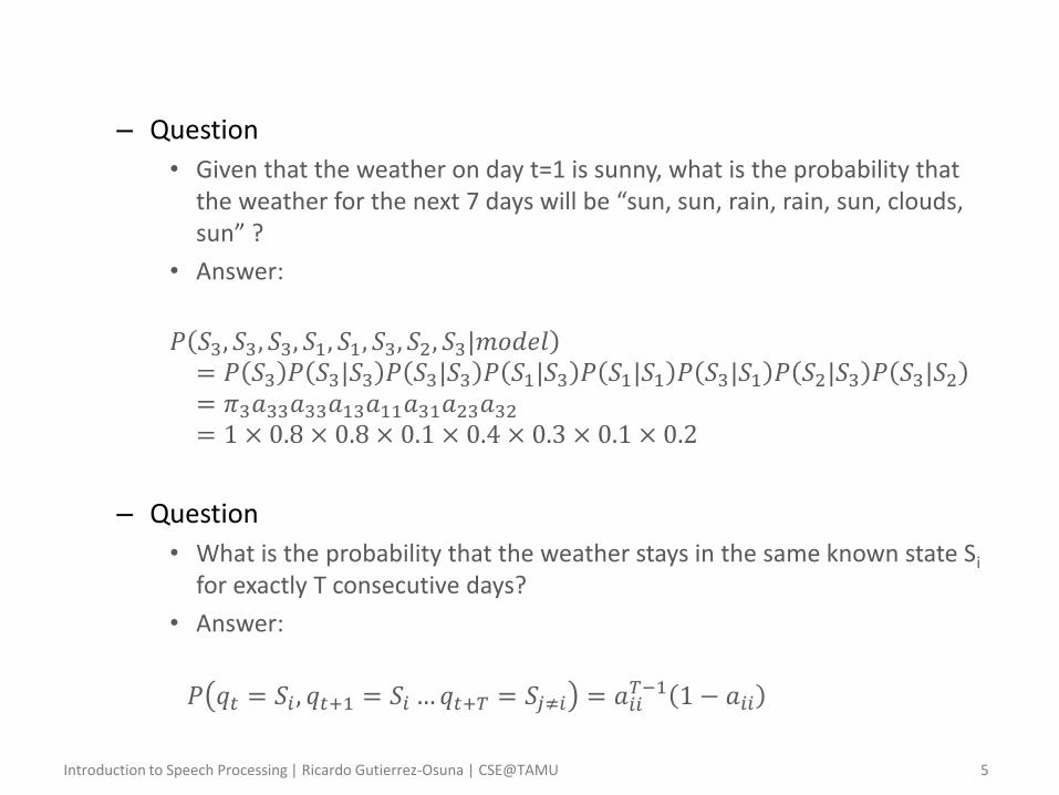
– Question
• Given that the weather on day t=1 is sunny, what is the probability that the weather for the next 7 days will be “sun, sun, rain, rain, sun, clouds, sun” ?
• Answer:
𝑃 𝑆3, 𝑆3, 𝑆3, 𝑆1, 𝑆1, 𝑆3, 𝑆2, 𝑆3|𝑚𝑜𝑑𝑒𝑙= 𝑃 𝑆3 𝑃 𝑆3|𝑆3 𝑃 𝑆3|𝑆3 𝑃 𝑆1|𝑆3 𝑃 𝑆1|𝑆1 𝑃 𝑆3|𝑆1 𝑃 𝑆2|𝑆3 𝑃 𝑆3|𝑆2= 𝜋3𝑎33𝑎33𝑎13𝑎11𝑎31𝑎23𝑎32= 1 × 0.8 × 0.8 × 0.1 × 0.4 × 0.3 × 0.1 × 0.2
– Question
• What is the probability that the weather stays in the same known state Si for exactly T consecutive days?
• Answer:
𝑃 𝑞𝑡 = 𝑆𝑖 , 𝑞𝑡+1 = 𝑆𝑖 …𝑞𝑡+𝑇 = 𝑆𝑗≠𝑖 = 𝑎𝑖𝑖𝑇−1 1 − 𝑎𝑖𝑖
Introduction to Speech Processing | Ricardo Gutierrez-Osuna | CSE@TAMU 6
Hidden Markov models
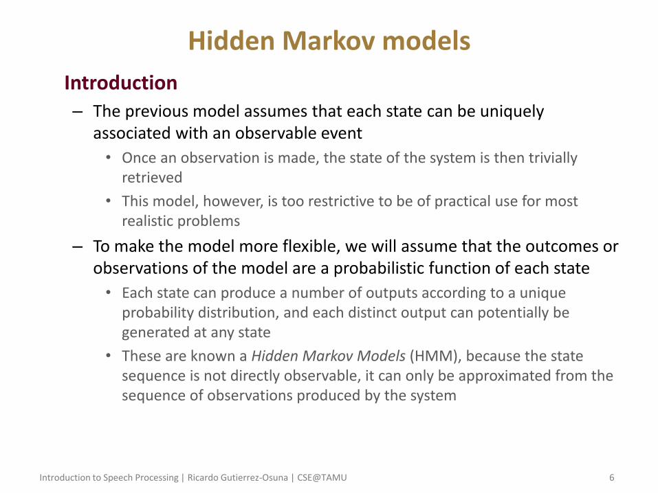
• Introduction – The previous model assumes that each state can be uniquely
associated with an observable event
• Once an observation is made, the state of the system is then trivially retrieved
• This model, however, is too restrictive to be of practical use for most realistic problems
– To make the model more flexible, we will assume that the outcomes or observations of the model are a probabilistic function of each state
• Each state can produce a number of outputs according to a unique probability distribution, and each distinct output can potentially be generated at any state
• These are known a Hidden Markov Models (HMM), because the state sequence is not directly observable, it can only be approximated from the sequence of observations produced by the system
Introduction to Speech Processing | Ricardo Gutierrez-Osuna | CSE@TAMU 7
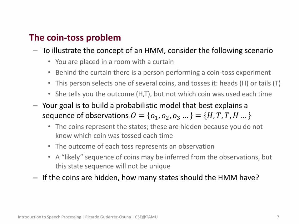
• The coin-toss problem – To illustrate the concept of an HMM, consider the following scenario
• You are placed in a room with a curtain
• Behind the curtain there is a person performing a coin-toss experiment
• This person selects one of several coins, and tosses it: heads (H) or tails (T)
• She tells you the outcome (H,T), but not which coin was used each time
– Your goal is to build a probabilistic model that best explains a sequence of observations 𝑂 = 𝑜1, 𝑜2, 𝑜3… = 𝐻, 𝑇, 𝑇, 𝐻 …
• The coins represent the states; these are hidden because you do not know which coin was tossed each time
• The outcome of each toss represents an observation
• A “likely” sequence of coins may be inferred from the observations, but this state sequence will not be unique
– If the coins are hidden, how many states should the HMM have?

Introduction to Speech Processing | Ricardo Gutierrez-Osuna | CSE@TAMU 8
– One-coin model • In this case, we assume that the person behind
the curtain only has one coin
• As a result, the Markov model is observable since there is only one state
• In fact, we may describe the system with a deterministic model where the states are the actual observations (see figure)
• In either case, the model parameter P(H) may be found from the ratio of heads and tails
– Two-coin model • A more sophisticated HMM would be to
assume that there are two coins – Each coin (state) has its own distribution of
heads and tails, to model the fact that the coins may be biased
– Transitions between the two states model the random process used by the person behind the curtain to select one of the coins
• The model has 4 free parameters
[Rabiner, 1989]
Introduction to Speech Processing | Ricardo Gutierrez-Osuna | CSE@TAMU 9
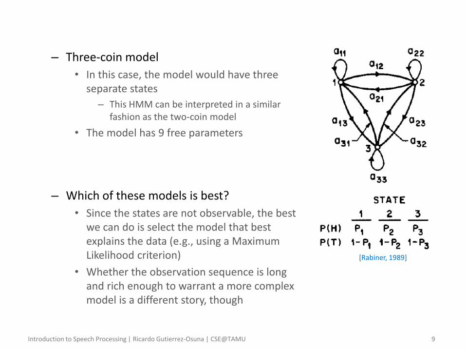
– Three-coin model
• In this case, the model would have three separate states
– This HMM can be interpreted in a similar fashion as the two-coin model
• The model has 9 free parameters
– Which of these models is best?
• Since the states are not observable, the best we can do is select the model that best explains the data (e.g., using a Maximum Likelihood criterion)
• Whether the observation sequence is long and rich enough to warrant a more complex model is a different story, though
[Rabiner, 1989]

Introduction to Speech Processing | Ricardo Gutierrez-Osuna | CSE@TAMU 10
• The urn-ball problem – To further illustrate the concept of an HMM, consider this scenario
• You are placed in the same room with a curtain
• Behind the curtain there are N urns, each containing a large number of balls from M different colors
• The person behind the curtain selects an urn according to an internal random process, then randomly grabs a ball from the selected urn
• He shows you the ball, and places it back in the urn
• This process is repeated over and over
– Questions
• How would you represent this experiment with an HMM? What are the states? Why are the states hidden? What are the observations?
Urn 1 Urn 2 Urn N

Introduction to Speech Processing | Ricardo Gutierrez-Osuna | CSE@TAMU 11
• Elements of an HMM – An HMM is characterized by the following set of parameters
• 𝑁, the number of states in the model 𝑆 = 𝑆1, 𝑆2…𝑆𝑁
• 𝑀, the number of discrete observation symbols 𝑉 = 𝑣1, 𝑣2…𝑣𝑀
• 𝐴 = 𝑎𝑖𝑗 , the state transition probability
𝑎𝑖𝑗 = 𝑃 𝑞𝑡+1 = 𝑆𝑗|𝑞𝑡 = 𝑆𝑖
• 𝐵 = 𝑏𝑗 𝑘 , the observation or emission probability distribution
𝑏𝑗 𝑘 = 𝑃 𝑜𝑡 = 𝑣𝑘|𝑞𝑡 = 𝑆𝑗
• 𝜋, the initial state distribution
𝜋𝑗 = 𝑃 𝑞1 = 𝑆𝑗
– Therefore, an HMM is specified by two scalars (𝑁 and 𝑀) and three probability distributions (𝐴,𝐵, and 𝜋)
• In what follows, we will represent an HMM by the compact notation 𝜆 = 𝐴, 𝐵, 𝜋
Introduction to Speech Processing | Ricardo Gutierrez-Osuna | CSE@TAMU 12
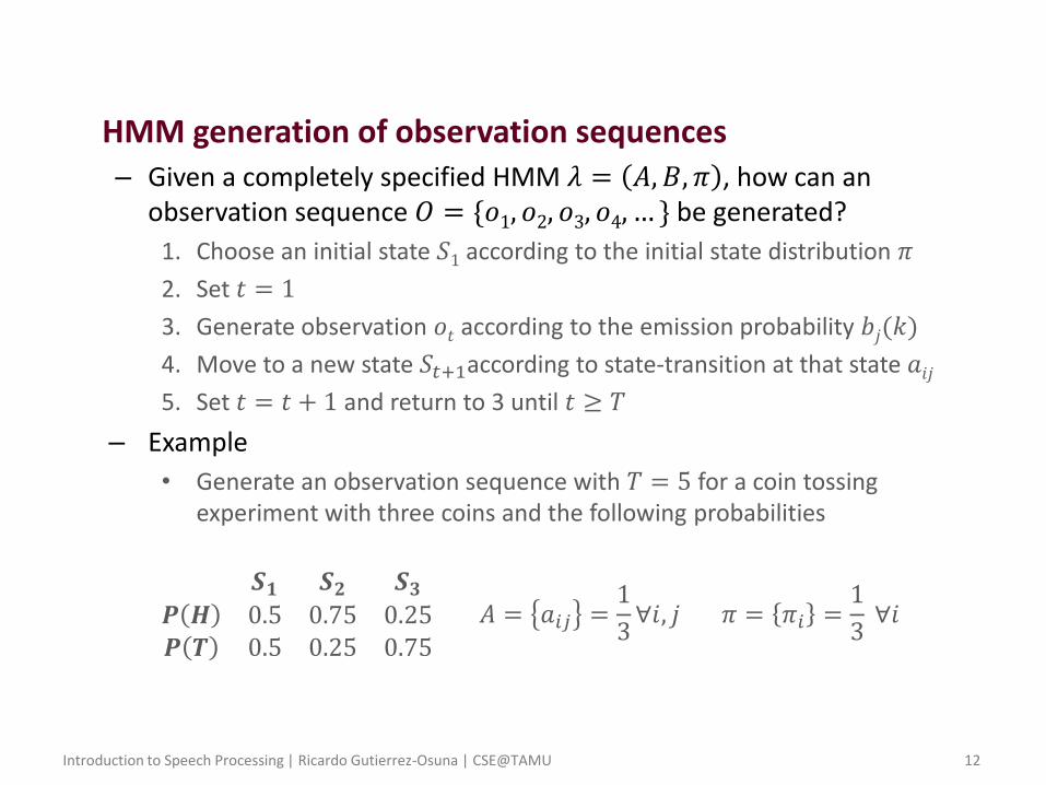
• HMM generation of observation sequences – Given a completely specified HMM 𝜆 = 𝐴, 𝐵, 𝜋 , how can an
observation sequence 𝑂 = {𝑜1, 𝑜2, 𝑜3, 𝑜4, … } be generated?
1. Choose an initial state 𝑆1 according to the initial state distribution 𝜋
2. Set 𝑡 = 1
3. Generate observation 𝑜𝑡 according to the emission probability 𝑏𝑗(𝑘)
4. Move to a new state 𝑆𝑡+1according to state-transition at that state 𝑎𝑖𝑗
5. Set 𝑡 = 𝑡 + 1 and return to 3 until 𝑡 ≥ 𝑇
– Example
• Generate an observation sequence with 𝑇 = 5 for a coin tossing experiment with three coins and the following probabilities
𝑺𝟏 𝑺𝟐 𝑺𝟑
𝑷 𝑯 0.5 0.75 0.25𝑷 𝑻 0.5 0.25 0.75
𝐴 = 𝑎𝑖𝑗 =1
3∀𝑖, 𝑗 𝜋 = 𝜋𝑖 =
1
3 ∀𝑖
Introduction to Speech Processing | Ricardo Gutierrez-Osuna | CSE@TAMU 13
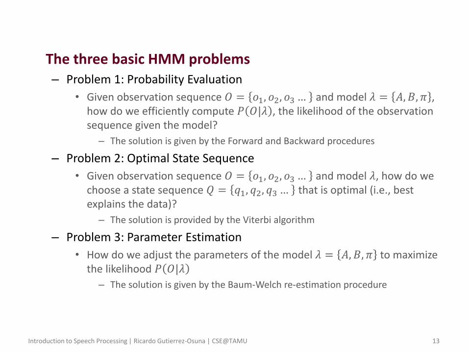
• The three basic HMM problems – Problem 1: Probability Evaluation
• Given observation sequence 𝑂 = 𝑜1, 𝑜2, 𝑜3… and model 𝜆 = 𝐴, 𝐵, 𝜋 , how do we efficiently compute 𝑃 𝑂|𝜆 , the likelihood of the observation sequence given the model?
– The solution is given by the Forward and Backward procedures
– Problem 2: Optimal State Sequence
• Given observation sequence 𝑂 = 𝑜1, 𝑜2, 𝑜3… and model 𝜆, how do we choose a state sequence 𝑄 = 𝑞1, 𝑞2, 𝑞3… that is optimal (i.e., best explains the data)?
– The solution is provided by the Viterbi algorithm
– Problem 3: Parameter Estimation
• How do we adjust the parameters of the model 𝜆 = 𝐴, 𝐵, 𝜋 to maximize the likelihood 𝑃 𝑂|𝜆
– The solution is given by the Baum-Welch re-estimation procedure
Introduction to Speech Processing | Ricardo Gutierrez-Osuna | CSE@TAMU 14
Forward and Backward procedures
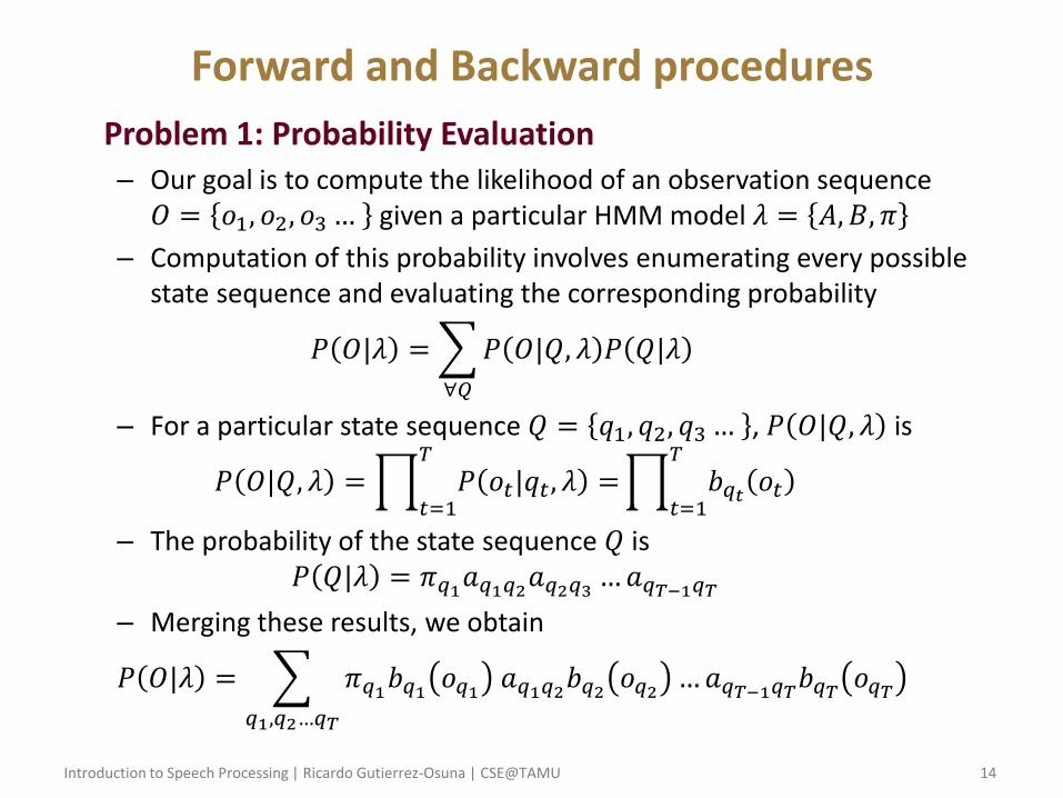
• Problem 1: Probability Evaluation – Our goal is to compute the likelihood of an observation sequence 𝑂 = 𝑜1, 𝑜2, 𝑜3… given a particular HMM model 𝜆 = 𝐴, 𝐵, 𝜋
– Computation of this probability involves enumerating every possible state sequence and evaluating the corresponding probability
𝑃 𝑂|𝜆 = 𝑃 𝑂|𝑄, 𝜆 𝑃 𝑄|𝜆
∀𝑄
– For a particular state sequence 𝑄 = 𝑞1, 𝑞2, 𝑞3… , 𝑃 𝑂|𝑄, 𝜆 is
𝑃 𝑂|𝑄, 𝜆 = 𝑃 𝑜𝑡|𝑞𝑡, 𝜆 =𝑇
𝑡=1 𝑏𝑞𝑡 𝑜𝑡
𝑇
𝑡=1
– The probability of the state sequence 𝑄 is 𝑃 𝑄|𝜆 = 𝜋𝑞1𝑎𝑞1𝑞2𝑎𝑞2𝑞3 …𝑎𝑞𝑇−1𝑞𝑇
– Merging these results, we obtain
𝑃 𝑂|𝜆 = 𝜋𝑞1𝑏𝑞1 𝑜𝑞1 𝑎𝑞1𝑞2𝑏𝑞2 𝑜𝑞2 …𝑎𝑞𝑇−1𝑞𝑇𝑏𝑞𝑇 𝑜𝑞𝑇𝑞1,𝑞2…𝑞𝑇

Introduction to Speech Processing | Ricardo Gutierrez-Osuna | CSE@TAMU 15
– Computational complexity
• With 𝑁𝑇possible state sequences, this approach becomes unfeasible even for small problems… sound familiar?
– For 𝑁 = 5 and 𝑇 = 100, the order of computations is in the order of 1072
• Fortunately, the computation of 𝑃 𝑂|𝜆 has a lattice (or trellis) structure, which lends itself to a very efficient implementation known as the Forward procedure
[Rabiner, 1989]

Introduction to Speech Processing | Ricardo Gutierrez-Osuna | CSE@TAMU 16
• The Forward procedure – Consider the following variable 𝛼𝑡 𝑖 defined as
𝛼𝑡 𝑖 = 𝑃 𝑜1, 𝑜2…𝑜𝑡, 𝑞𝑡 = 𝑆𝑖|𝜆
• which represents the probability of the observation sequence up to time 𝑡 AND the state 𝑆𝑖 at time 𝑡, given model 𝜆
– Computation of this variable can be efficiently performed by induction
• Initialization: 𝛼1 𝑖 = 𝜋𝑖𝑏𝑖 𝑜1
• Induction: 𝛼𝑡+1 𝑗 = 𝛼𝑡 𝑖 𝑎𝑖𝑗𝑁𝑖=1 𝑏𝑗 𝑜𝑡+1
1 ≤ 𝑡 ≤ T − 1 1 ≤ 𝑗 ≤ 𝑁
• Termination: 𝑃 𝑂|𝜆 = 𝛼𝑇 𝑖𝑁𝑖=1
• As a result, computation of 𝑃 𝑂|𝜆 can be reduced from 2𝑇 × 𝑁𝑇 down to 𝑁2 × T operations (from 1072 to 3000 for 𝑁 = 5, 𝑇 = 100)
[Rabiner, 1989]

Introduction to Speech Processing | Ricardo Gutierrez-Osuna | CSE@TAMU 17
• The Backward procedure
– Analogously, consider the backward variable 𝛽𝑡 𝑖 defined as
𝛽𝑡 𝑖 = 𝑃 𝑜𝑡+1, 𝑜𝑡+2…𝑜𝑇|𝑞𝑡 = 𝑆𝑖 , 𝜆
– 𝛽𝑡 𝑖 represents the probability of the partial observation sequence from 𝑡 + 1 to the end, given state 𝑆𝑖 at time 𝑡 and model 𝜆
• As before, 𝛽𝑡 𝑖 can be computed through induction
• Initialization: 𝛽𝑇 𝑖 = 1 (arbitrarily)
• Induction: 𝛽𝑡 𝑖 = 𝑎𝑖𝑗𝑏𝑗 𝑜𝑡+1 𝛽𝑡+1 𝑗𝑁𝑗=1
𝑡 = 𝑇 − 1, 𝑇 − 2…11 ≤ 𝑖 ≤ 𝑁
– Similarly, this computation can be effectively performed in the order
of 𝑁2 × 𝑇 operations
[Rabiner, 1989]
Introduction to Speech Processing | Ricardo Gutierrez-Osuna | CSE@TAMU 18
The Viterbi algorithm
• Problem 2: Optimal State Sequence – Finding the optimal state sequence is more difficult problem that the
estimation of 𝑃 𝑂|𝜆
– Part of the issue has to do with defining an optimality measure, since several criteria are possible
• Finding the states 𝑞𝑡that are individually more likely at each time 𝑡
• Finding the single best state sequence path (i.e., maximize the posterior 𝑃 𝑂|𝑄, 𝜆
– The second criterion is the most widely used, and leads to the well-known Viterbi algorithm
• However, we first optimize the first criterion as it allows us to define a variable that will be used later in the solution of Problem 3

Introduction to Speech Processing | Ricardo Gutierrez-Osuna | CSE@TAMU 19
– As in the Forward-Backward procedures, we define a variable 𝛾𝑡 𝑖
𝛾𝑡 𝑖 = 𝑃 𝑞𝑡 = 𝑆𝑖|𝑂, 𝜆
• which represents the probability of being in state 𝑆𝑖 at time 𝑡, given the observation sequence 𝑂 and model
– Using the definition of conditional probability, we can write
𝛾𝑡 𝑖 = 𝑃 𝑞𝑡 = 𝑆𝑖|𝑂, 𝜆 =𝑃 𝑂, 𝑞𝑡 = 𝑆𝑖|𝜆
𝑃 𝑂|𝜆=
𝑃 𝑂, 𝑞𝑡 = 𝑆𝑖|𝜆
𝑃 𝑂, 𝑞𝑡 = 𝑆𝑖|𝜆𝑁𝑖=1
– Now, the numerator of 𝛾𝑡 𝑖 is equal to the product of 𝛼𝑡 𝑖 and 𝛽𝑡 𝑖
𝛾𝑡 𝑖 =𝑃 𝑂, 𝑞𝑡 = 𝑆𝑖|𝜆
𝑃 𝑂, 𝑞𝑡 = 𝑆𝑖|𝜆𝑁𝑖=1
=𝛼𝑡 𝑖 𝛽𝑡 𝑖
𝛼𝑡 𝑖 𝛽𝑡 𝑖𝑁𝑖=1
– The individually most likely state 𝑞𝑡∗ at each time is then
𝑞𝑡∗ = arg max
1≤𝑖≤𝑁𝛾𝑡 𝑖 ∀𝑡 = 1…𝑇

Introduction to Speech Processing | Ricardo Gutierrez-Osuna | CSE@TAMU 20
– The problem with choosing the individually most likely states is that the overall state sequence may not be valid
• Consider a situation where the individually most likely states are 𝑞𝑡 = 𝑆𝑖 and 𝑞𝑡+1 = 𝑆𝑗, but the transition probability 𝑎𝑖𝑗 = 0
– Instead, and to avoid this problem, it is common to look for the single best state sequence, at the expense of having sub-optimal individual states
– This is accomplished with the Viterbi algorithm

Introduction to Speech Processing | Ricardo Gutierrez-Osuna | CSE@TAMU 21
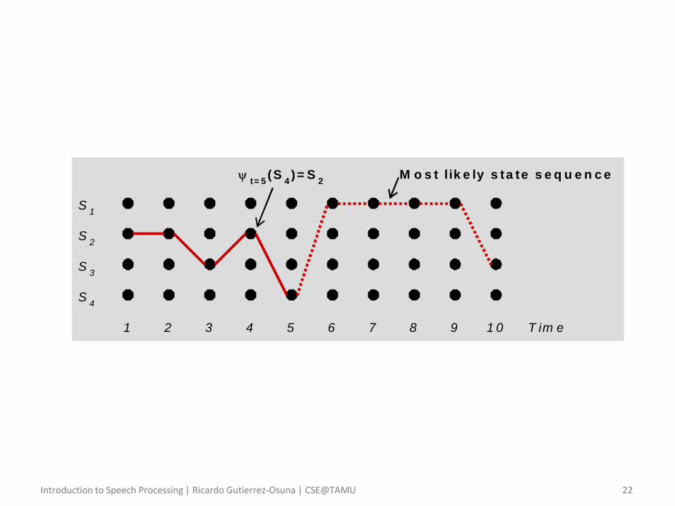
• The Viterbi algorithm – To find the single best state sequence we define yet another variable
𝛿𝑡 𝑖 = max𝑞1𝑞2…𝑞𝑡−1
𝑃 𝑞1𝑞2…𝑞𝑡 = 𝑆𝑖 , 𝑜1𝑜2…𝑜𝑡|𝜆
• which represents the highest probability along a single path that accounts for the first 𝑡 observations and ends at state 𝑆𝑖
– By induction, 𝛿𝑡+1 𝑗 can be computed as
𝛿𝑡+1 𝑗 = max𝑖
𝛿𝑡 𝑖 𝑎𝑖𝑗 𝑏𝑗 𝑜𝑡+1
– To retrieve the state sequence, we also need to keep track of the state that maximizes 𝛿𝑡 𝑖 at each time 𝑡, which is done by constructing an array
Ψ𝑡+1 𝑗 = arg max1≤𝑖≤𝑁
𝛿𝑡 𝑖 𝑎𝑖𝑗
• Ψ𝑡+1 𝑗 is the state at time 𝑡 from which a transition to state 𝑆𝑗 maximizes the probability 𝛿𝑡+1 𝑗
Introduction to Speech Processing | Ricardo Gutierrez-Osuna | CSE@TAMU 22
1 2 3 4 5 6 7 8 9 1 0
S1
S2
S3
S4
T im e
t= 5
(S4)= S
2M o s t lik e ly s ta te s e q u e n c e
1 2 3 4 5 6 7 8 9 1 0
S1
S2
S3
S4
T im e
t= 5
(S4)= S
2M o s t lik e ly s ta te s e q u e n c e
Introduction to Speech Processing | Ricardo Gutierrez-Osuna | CSE@TAMU 23
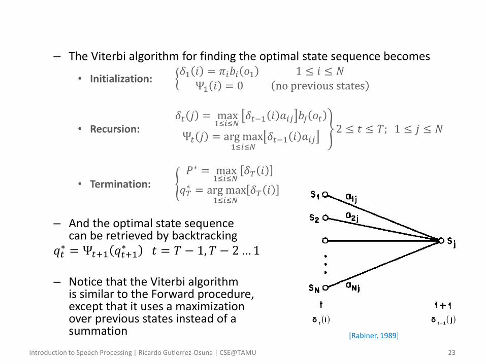
– The Viterbi algorithm for finding the optimal state sequence becomes
• Initialization: 𝛿1 𝑖 = 𝜋𝑖𝑏𝑖 𝑜1 1 ≤ 𝑖 ≤ 𝑁
Ψ1 𝑖 = 0 no previous states
• Recursion: 𝛿𝑡 𝑗 = max
1≤𝑖≤𝑁 𝛿𝑡−1 𝑖 𝑎𝑖𝑗 𝑏𝑗 𝑜𝑡
Ψ𝑡 𝑗 = arg max1≤𝑖≤𝑁
𝛿𝑡−1 𝑖 𝑎𝑖𝑗 2 ≤ 𝑡 ≤ 𝑇; 1 ≤ 𝑗 ≤ 𝑁
• Termination: 𝑃∗ = max
1≤𝑖≤𝑁 𝛿𝑇 𝑖
𝑞𝑇∗ = arg max
1≤𝑖≤𝑁 𝛿𝑇 𝑖
– And the optimal state sequence can be retrieved by backtracking
𝑞𝑡∗ = Ψ𝑡+1 𝑞𝑡+1
∗ 𝑡 = 𝑇 − 1, 𝑇 − 2…1
– Notice that the Viterbi algorithm is similar to the Forward procedure, except that it uses a maximization over previous states instead of a summation
iδt
jδ1t
[Rabiner, 1989]