kinematic robot calibration using a double...

Department of Automatic Control

Kinematic Robot Calibration Using a Double Ball-Bar

Sandra Collin

MSc Thesis ISRN LUTFD2/TFRT--6000--SE ISSN 0280-5316

Department of Automatic Control Lund University Box 118 SE-221 00 LUND Sweden

© 2016 by Sandra Collin. All rights reserved. Printed in Sweden by Tryckeriet i E-huset Lund 2016

Abstract

Calibration of robots is an essential part of industry today when there is a high accu-racy requirement. Several calibration methods have proven to be highly accurate butalso expensive and time consuming to use. In this thesis a new calibration methodhas been developed. The method does not depend on any external measurement sys-tems but instead rely entirely on the robot’s own sensors. The method is based ona closed loop system where a robot is connected to a double ball-bar attached to arigid point. The ball-bar creates a constraint restraining the robot to a spherical sur-face. All measured joint positions are fitted to the sphere by altering the geometricrepresentation of the robot. The issues with the method proved to be the processeffects as well as dynamic effects influencing the joints and links resulting in in-correctly measured joint positions. Some of these unwanted effects were filtered byapplying the clamping method to estimate the joint characteristics. When the newrobot geometry was identified, a verification was performed. The verification re-sulted in an improved positioning of almost 80 % and an improved orientation of23 % compared to the initial robot geometry.

3

Acknowledgements

First of all I would like to thank Anders Robertsson for being a motivating professorwith a great passion for robotics. I have had the pleasure of having Anders as myprofessor which introduced and made me interested in robotics.

I would like to extend my gratitude to my two supervisors at the Departmentof Automatic Control at Lund University, Anders Robertsson and Björn Olofssonfor their knowledge and help in the area of robotics. Special thanks to Björn for hisconstant mentoring and for always coming to my rescue, even if help was neededon weekends. Furthermore, I want to thank my supervisors at Cognibotics AB, KlasNilsson and Mathias Haage for giving me the opportunity to perform this masterthesis. Their inputs and discussion have been valuable throughout the thesis.

5

Contents

List of Figures 9List of Tables 111. Introduction 13

1.1 Motivation . . . . . . . . . . . . . . . . . . . . . . . . . . . . . 131.2 Problem formulation . . . . . . . . . . . . . . . . . . . . . . . . 141.3 Outline . . . . . . . . . . . . . . . . . . . . . . . . . . . . . . . 15

2. Robot calibration 162.1 Repeatability and accuracy . . . . . . . . . . . . . . . . . . . . 162.2 Calibration process . . . . . . . . . . . . . . . . . . . . . . . . 182.3 Previous work . . . . . . . . . . . . . . . . . . . . . . . . . . . 22

3. Kinematic identification 243.1 Closed-loop system . . . . . . . . . . . . . . . . . . . . . . . . 243.2 Spherical movement . . . . . . . . . . . . . . . . . . . . . . . . 253.3 Least-squares minimization . . . . . . . . . . . . . . . . . . . . 263.4 Scalability . . . . . . . . . . . . . . . . . . . . . . . . . . . . . 283.5 Identifiable parameters . . . . . . . . . . . . . . . . . . . . . . . 303.6 Dynamic effects . . . . . . . . . . . . . . . . . . . . . . . . . . 35

4. Simulation 384.1 Preliminaries . . . . . . . . . . . . . . . . . . . . . . . . . . . . 384.2 Simulation software . . . . . . . . . . . . . . . . . . . . . . . . 394.3 Simulation results . . . . . . . . . . . . . . . . . . . . . . . . . 43

5. Experiments 475.1 Setup . . . . . . . . . . . . . . . . . . . . . . . . . . . . . . . . 475.2 Experiment . . . . . . . . . . . . . . . . . . . . . . . . . . . . . 495.3 Dynamic identification . . . . . . . . . . . . . . . . . . . . . . . 515.4 Kinematic identification . . . . . . . . . . . . . . . . . . . . . . 525.5 Verification . . . . . . . . . . . . . . . . . . . . . . . . . . . . . 54

6. Conclusion and discussion 626.1 Further work . . . . . . . . . . . . . . . . . . . . . . . . . . . . 62

7

Contents

A. Kinematics 65A.1 Rigid body transformations . . . . . . . . . . . . . . . . . . . . 65A.2 Denavit-Hartenberg . . . . . . . . . . . . . . . . . . . . . . . . 66A.3 Kinematics . . . . . . . . . . . . . . . . . . . . . . . . . . . . . 67

B. Robots 68B.1 Robot descriptions . . . . . . . . . . . . . . . . . . . . . . . . . 68B.2 DH parameters . . . . . . . . . . . . . . . . . . . . . . . . . . . 70

Bibliography 71

8

List of Figures

2.1 Repeatability and accuracy when repeatably moving toward a given pose 162.2 Representation of backlash in a gearbox [Planetary Gearbox Glossary] 172.3 Beam deflection . . . . . . . . . . . . . . . . . . . . . . . . . . . . . 182.4 Hayati’s Extended Denavit Hartenberg convention [Hayati and Mirmi-

rani, 1985] . . . . . . . . . . . . . . . . . . . . . . . . . . . . . . . . 20

3.1 Closed loop system . . . . . . . . . . . . . . . . . . . . . . . . . . . 243.2 Ball-bar on a sphere . . . . . . . . . . . . . . . . . . . . . . . . . . . 253.3 Spherical and cartesian coordinates . . . . . . . . . . . . . . . . . . . 263.4 Plotted poses for a data set . . . . . . . . . . . . . . . . . . . . . . . 273.5 Plottet poses for a dataset near the sphere surface . . . . . . . . . . . 283.6 Scalability issue . . . . . . . . . . . . . . . . . . . . . . . . . . . . . 293.7 Ball-bar length estimation . . . . . . . . . . . . . . . . . . . . . . . . 303.8 Global/local minima issue . . . . . . . . . . . . . . . . . . . . . . . 343.9 Joint-model containing backlash, friction and nonlinear joint stiffness

[Lehmann et al., 2013] . . . . . . . . . . . . . . . . . . . . . . . . . 353.10 Theoretical clamping curve [Gear Backlash] . . . . . . . . . . . . . . 363.11 Real clamping curve [Gear Backlash] . . . . . . . . . . . . . . . . . 373.12 Friction curve according to [Bittencourt et al., 2010] . . . . . . . . . 37

4.1 Block diagram of the software for simulation and experiments . . . . 394.2 Model of the shadow robot for the IRB6640 and the ball-bar in Robot-

Studio. . . . . . . . . . . . . . . . . . . . . . . . . . . . . . . . . . . 404.3 To the left is a geometric CAD-model of the gimbal joint and to the

right the real joint is shown. . . . . . . . . . . . . . . . . . . . . . . . 404.4 Example on how the robot re-orients during a spiral . . . . . . . . . . 424.5 Spiral-program generated through the add-in in RobotStudio . . . . . 424.6 Program generated through the add-in in RobotStudio . . . . . . . . . 44

5.1 Setup of IRB140 in RobotLab . . . . . . . . . . . . . . . . . . . . . 48

9

List of Figures

5.2 Setup of IRB140 in RobotStudio . . . . . . . . . . . . . . . . . . . . 485.3 RSP clamping device . . . . . . . . . . . . . . . . . . . . . . . . . . 505.4 Unlocked RSP . . . . . . . . . . . . . . . . . . . . . . . . . . . . . . 505.5 Fastening of the gimbal joint . . . . . . . . . . . . . . . . . . . . . . 515.6 Clamping curves for IRB140. . . . . . . . . . . . . . . . . . . . . . . 525.7 Friction curve for joint 2 of IRB140 . . . . . . . . . . . . . . . . . . 535.8 Position of the fixed point during an experiment . . . . . . . . . . . . 545.9 Diodes to define the TCP pose . . . . . . . . . . . . . . . . . . . . . 575.10 Square-path for verification . . . . . . . . . . . . . . . . . . . . . . . 575.11 Verification result for the nominal and real curves . . . . . . . . . . . 585.12 Verification result for the nominal, identified and real curves . . . . . 595.13 Verification result for the nominal, identified parameters filtered from

dynamic effects and real curves . . . . . . . . . . . . . . . . . . . . . 60

A.1 Homogeneous transform [Freidovich, 2013] . . . . . . . . . . . . . . 66A.2 DH notation for the four parameters [Freidovich, 2013] . . . . . . . . 67

B.1 Geometric description of IRB6640 in mm [Product manual IRB6640] 68B.2 Geometric description of IRB140 in mm [Product manual IRB140] . . 69

10

List of Tables

3.1 Identifiable DH and ball-bar parameters (-: identifiable, n: non-identifiable, 0: non-identifiable with zero jacobian ) . . . . . . . . . . 31

3.2 Impact on parameters when d1 is fixed with an error (f: fixed, e: error,-: not affected, a: affected ) . . . . . . . . . . . . . . . . . . . . . . . 31



3.5 Impact on parameters when θ1 is fixed with an error (f: fixed, e: error,-: not affected, a: affected ) . . . . . . . . . . . . . . . . . . . . . . . 33



3.8 Impact on parameters when lr is fixed with an error (f: fixed, e: error, -:not affected, a: affected ) . . . . . . . . . . . . . . . . . . . . . . . . 34

4.1 Identified values for the IRB140 simulation under optimal conditionwith known ball-bar length . . . . . . . . . . . . . . . . . . . . . . . 45

4.2 Identified values for the IRB140 simulation under two sets of measure-ment noise. . . . . . . . . . . . . . . . . . . . . . . . . . . . . . . . 46

5.1 Spring constants for the IRB140 . . . . . . . . . . . . . . . . . . . . 525.2 Identified errors from identification without dynamic effects and with a

known rod length. All units are in µm except for α1 and θi which arein mrad. . . . . . . . . . . . . . . . . . . . . . . . . . . . . . . . . . 53

5.3 Identified errors from identification with dynamic effects and with aknown rod length. All units are in µm except for α1 and θi which arein mrad. . . . . . . . . . . . . . . . . . . . . . . . . . . . . . . . . . 54

5.4 Residuals for the sphere fitting of the rod length . . . . . . . . . . . . 55

11

List of Tables

5.5 Deviations from the path using nominal parameters . . . . . . . . . . 585.6 Deviations from the path using identified parameters . . . . . . . . . 595.7 Deviations from the path using identified parameters filtered from dy-

namic effects . . . . . . . . . . . . . . . . . . . . . . . . . . . . . . 61

B.1 Joint limits for IRB6640 . . . . . . . . . . . . . . . . . . . . . . . . 69B.2 Joint limits IRB140 . . . . . . . . . . . . . . . . . . . . . . . . . . . 70B.3 DH parameters in m/rad for the IRB6640 . . . . . . . . . . . . . . . 70B.4 DH parameters in m/rad for the IRB140 . . . . . . . . . . . . . . . . 70

12

1Introduction

1.1 Motivation

It is today becoming more and more desirable to use robots in industry and the de-mand for higher precision has increased. Robots are often used in automation whenthere is a high tolerance demand, the environment is dangerous or when there is aneed for efficient production. The accuracy of the robot is not important when therobot’s end effector is manually taught, for example in a pick-and-place applica-tion where the poses are constant, but rather it is the repeatability that defines theprecision of the system. When using offline programming the positions are createdin a virtual space and therefore accuracy becomes important. The robot’s absoluteaccuracy is seldom specified by the manufacturer and tend to be rather inaccurate.Fortunately, the robot can be calibrated to increase the accuracy given a high re-peatability which in today’s robots is rather common.

To achieve increased accuracy through calibration, external equipments are of-ten used for measuring positions in space which are used to identify the robot’sgeometric parameters. The equipments are often expensive, large, difficult to installand time consuming to use. If it is possible to identify the robot’s properties withenough precision using only the robot’s own sensors, the industrial usage of highprecision robots can increase significantly due to easier and more cost efficient cal-ibration. This is exactly what Cognibotics AB intends to accomplish. CogniboticsAB is a Swedish company located in Lund and has developed a method for dynamicrobot calibration called the clamping method. The method is used to compensate fordeviations between the real and the nominal robot and thereby increase the accuracy.What is remarkable about the clamping method is that the properties of the robot’sjoints are identified when the end effector is clamped to a rigid environment, usingonly the robot’s internal sensors for measurement. The clamping method is used toestimate the non geometric properties of the robot, such as backlash, friction andjoint stiffness. A new method is proposed to identify the geometric parameters ofthe robot using the robot’s internal sensors together with a stiff double ball-bar. Thismethod is to be further developed and verified.

13

Chapter 1. Introduction

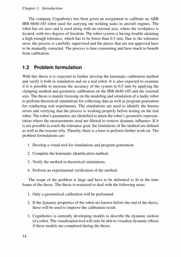
The company Cognibotics has been given an assignment to calibrate an ABBIRB 6640-185 robot used for carrying out welding tasks in aircraft engines. Therobot has six axes and is used along with an external axis, where the workpiece islocated, with two degrees of freedom. The robot system is having trouble attaininga high enough tolerance, which has to be lower than 0.5 mm. Due to the toleranceerror, the process is carefully supervised and the pieces that are not approved haveto be manually corrected. The process is time consuming and have much to benefitfrom calibration.

1.2 Problem formulation

With this thesis it is expected to further develop the kinematic calibration methodand verify it both in simulation and on a real robot. It is also expected to examineif it is possible to increase the accuracy of the system to 0.5 mm by applying theclamping method and geometric calibration on the IRB 6640-185 and the externalaxis. The thesis is mainly focusing on the modeling and simulation of a faulty robotto perform theoretical simulations for collecting data as well as program generationfor conducting real experiments. The simulations are used to identify the knownerrors and verifying that the process is working properly before testing on the realrobot. The robot’s parameters are identified to attain the robot’s geometric represen-tation where the measurements used are filtered to remove dynamic influence. If itis not possible to reach the tolerance goal, the limitations of the method are definedas well as the reasons why. Thereby, there is a base to perform further work on. Theproblem formulations are:

1. Develop a visual tool for simulations and program generation.

2. Complete the kinematic identification method.

3. Verify the method in theoretical simulations.

4. Perform an experimental verification of the method.

The scope of the problem is large and have to be delimited to fit in the timeframe of the thesis. The thesis is restricted to deal with the following areas:

1. Only a geometrical calibration will be performed.

2. If the dynamic properties of the robot are known before the end of the thesis,these will be used to improve the calibration result.

3. Cognibotics is currently developing models to describe the dynamic motionof a robot. The visualization tool will only be able to visualize dynamic effectsif these models are completed during the thesis.

14

1.3 Outline

1.3 Outline

The outline of the report is as follows:

Chapter 2 addresses the area of robot calibration and why it is necessary. In thischapter different calibration methods are discussed.

Chapter 3 describes the developed kinematic identification model and it’s limita-tions.

Chapter 4 presents the software created for generating programs and simulations.The chapter also contains tests and results from simulations.

Chapter 5 describes the process used during experiments and presents the result.

Chapter 6 contains discussion and further work.

Appendix discloses the robot kinematics and the robot descriptions.

15

2Robot calibration

2.1 Repeatability and accuracy

The precision of a robot is defined using the terms repeatability and accuracy. Therepeatability of a robot describes how well a taught pose in space can be repeatablyreached and the accuracy how well the robot reaches a defined pose. In Fig. 2.1 theconcepts of repeatability and accuracy are shown. Poor repeatability can be seen astargets being widely spread around a specified pose and poor accuracy as targetsconcentrated around the wrong pose. The lower left figure corresponds to today’srobot systems.

Figure 2.1 Repeatability and accuracy when repeatably moving toward a givenpose

Programming a robot can be carried out in two ways: manually teaching thetargets in online programming and programming targets in a virtual environment,

16

2.1 Repeatability and accuracy

called offline programming. In applications where the pose is constant, good re-peatability of the robot makes it possible to manually teach the pose to where therobot should move. In offline programming it is of great importance to have a goodaccuracy. When programming offline the targets are defined in a virtual environ-ment where the targets are created using the robot’s nominal parameters. Thereforeit is not enough to only have good repeatability, good accuracy is also desirable.

Robot accuracyWhen referring to errors between the nominal and real robot there are mainly fivesources causing the errors [Nubiola and Bonev, 2014]: environmental (due to tem-perature variations during the warm up procedure), parametric (because of errors inthe kinematic parameters during manufacturing or assembly), measurement (reso-lution in the motor encoders), computational (round-offs) and applicational (errorsduring installation).

In this thesis, the errors compensated for are the parametric errors with filteringfrom dynamic effects. The dynamic errors used in the calibration are due to gravi-tation, tools and other instruments effects on the robot that depend on the stiffnessof the joints as well as friction causing the position of the tool to deviate from thedesired position. Some of the dynamic parameters influencing the position of therobot can be described as:

Backlash:

– When backlash occurs parts of a motion is lost due to gaps in the gearbox.Backlash is described as the maximum distance or angle a mechanical partis moved before contact is enforced to the next part and is represented inFig. 2.2. The reason for having backlash in a gearbox is to avoid the cogexperiencing friction on both sides to attain a smooth movement.

Figure 2.2 Representation of backlash in a gearbox [Planetary Gearbox Glossary]

17

Chapter 2. Robot calibration

Friction:

– Friction occurs when the joints are moved and is affected by load, speed ortemperature. Friction can be described as dependent on the tangential forcebetween two materials or substances in contact.

Link stiffness:

– The stiffness of the robot links determine how much the links are bent, com-pressed or extended when force is applied. Gravity and mass of the links andtool contributes to increased forces on the links. The links can be comparedto a beam being bent as can be seen in Fig. 2.2, where F is the force appliedwhich depends on the gravity and the mass of the beam.

Figure 2.3 Beam deflection

Joint stiffness:

– Since the encoders measuring the joint positions often are located on the mo-tor shaft instead of directly on the joint, the joint positions are calculatedusing motor positions and the stiffness of the joints have to be accounted for.The stiffness of the robot’s joints can be described as the ratio between themotor position and the motor torques of the joints causing the measured jointpositions to deflect from the actual joint positions.

2.2 Calibration process

As previously described calibrating a robot is performed with the intention of in-creasing the robot’s absolute accuracy. Calibration of a robot is usually performedby externally measuring the tool center point (TCP) in various positions with whicha new kinematic model can be built. To identify a new kinematic model these val-ues are compared to how the nominal robot should have behaved in the positionsby applying the measured joint positions to acknowledge the nominal pose. Thedifference between the measured and the nominal values is the error to which is tobe compensated for. The current nominal kinematic model is then replaced with the

18


new, more accurate, kinematic model. The steps for setting up a calibration are tochoose the kinematic model, the measurement system and the identification algo-rithm.

Kinematic model:There are several models and properties to take into consideration when decidingwhich kinematic model to use. There are mainly two properties used to define thekinematic model: completeness and parametrically continuous. For a model to becomplete it has to have a minimum of [Everett et al., 1987]: 4N + 2P + 6 independentkinematic parameters, where N denotes the number of degrees of freedom and Pthe number of prismatic joints. Parametrically continuous means that continuouschanges in joint positions should result in continuous changes in robot parameters.Thus should the model not contain any singularities.

Denavit-Hartenberg: The most commonly used model is the Denavit-Hartenberg(DH) convention because of it’s straightforward and simple approach. The DH con-vention is well documented and it is easy to find specified DH parameters for dif-ferent robots. The DH model is not complete since it only has 24 parameters, 4 forevery joint, and it is not parametrically continuous because of a singularity arisingwhen link 2 and 3 are nearly parallel [Zhuang et al., 1993]. The singularity causessmall variations in joint positions to result in parameter jumps in the DH model. Adetailed description of the DH convention can be found in Appendix A.

Other methods have been developed which extend the DH model to achievecompleteness. An example of such models is the S-model [Stone, 1987], where twoparameters are added to allow arbitrary position of the link frames. Another exampleis the zero-reference model [Moorning et al., 1991], which first establishes a basecoordinate system whereafter the values for the direction vector of each axis aredetermined when the robot is in its zero position. Both these models are extensionsof the DH model and are made complete but do not remove the singularity and arestill parametrically discontinuous.

Hayati extended DH [Hayati and Mirmirani, 1985]: In the extended DH con-vention developed by Hayati and Mirmirami an extra rotation parameter is addedto represent a small offset between two parallel axes, preventing them from beingparallel. This rotation parameter β results in a parametrically continuous kinematicconvention which removes the singularity present in the DH convention. The pa-rameter β can be seen in Fig. 2.4.

19


Figure 2.4 Hayati’s Extended Denavit Hartenberg convention [Hayati and Mirmi-rani, 1985]

Sheth and Uicker [Sheth and Uicker, 1972]: Separates joint movements from thelink geometries by introducing one frame for every joint and one for every link. Themodel is complete and parametrically continuous but has redundant parameters thatare hard to eliminate.

Roberts singular-free line presentation [Roberts, 1988]: The model has four pa-rameters for every joint, two for orientation and two for position. The model hasno singularities or special cases and is therefore parametrically continuous. It hasas many parameters as the DH model which makes it incomplete. One disadvan-tage is that all parameters are specified in a local coordinate system and have to betransformed to a common global coordinate system.

CPC [Sheth and Uicker, 1972]: CPC is a convention that uses Robert’s line rep-resentation to ensure parametrical continuity and adds two parameters to make itcomplete by implementing the S-model. The CPC is easy to use but has limiteddocumentation and specified parameters for different robots are hard to find.

Measurement systemThe measurement system is used for measuring the desired properties of the robot,for example the robot flange pose. The measurement equipment has a large effecton the precision of the calibration. The more accurate the measurement system is,the more accurate calibration is achieved. Examples of measurement systems are:

- A telescopic ball-bar to measure a radial distance [Nubiola and Bonev, 2014]with an accuracy better than ± 3.18 µm.

- A laser tracker with a specified accuracy of 22 µm at a range of 2 m [Nubiolaand Bonev, 2013].

- A CMM which calculates the least-squares estimate to the center of the spher-ical tooling ball with an inaccuracy of 12.1 µm over the entire workspace[Lightcap et al., 2008].

20


Calibration type:The extent of the calibration must be considered when performing a calibration.There are three levels of calibration [Everett et al., 1987]:

Level-1: Can also be referred to as the "joint-level" calibration where the error be-tween the desired joint position and the actual measured joint position is minimized.The calibration includes calibration of the joint sensors.

Level-2: Calibrates geometric errors of the kinematic model that may haveemerged during manufacturing or assembly of the parts.

Level-3: Includes non geometric dynamic calibration to compensate for errorssuch as backlash, friction and joint stiffness.

The goal of the thesis is to primarily conduct a level-2 simulated calibration withthe visualization tool. When calibrating the real robot, dynamic measurements areavailable and the measurements can be filtered to remove the dynamic effects.

Identification:There are several numerical algorithms used for minimizing the errors to identifythe parameters based on the collected measurements. One widely used algorithm forsolving nonlinear least-squares problems is the Levenberg-Marquardt method. Themethod is a combination of the Gauss-Newton and the steepest descent method. Thegoal is to minimize the sum of squares of the errors between the function and themeasured data set. Given a set of data, minimize the sum of squares of the deviationsto estimate the parameters β .

S(β ) =m

∑i=1

[yi− f (xi,β )]2 (2.1)

The steepest descent method [Fang, 2004] The steepest descent (SD) methodupdates parameters in the calculated gradient direction. It uses one dimension searchto iteratively find the minimum of the function and can be expressed as:

xk+1 = xk−λk5F(xk) (2.2)

SD is a robust method where the initial guess can be far away from the cor-rect values. However, since it uses a first-order derivative it can experience slowconvergence, especially when using larger functions.

The Newton method [Fang, 2004] In the Newton method a second-order deriva-tive function in the form of a Hessian matrix is used. The Hessian matrix is com-posed of the second-order partial derivatives of the function. The introduction of asecond-order derivative leads to faster convergence but at the expense of robustness,resulting in higher sensitivity for the initial guess.

21


xk+1 = xk− [H f (xk)]−15F(xk) (2.3)

The Gauss-Newton method [Fang, 2004] Since not all applications can computethe Hessian matrix, the Newton method was modified to form the Gauss-Newton(GN) method. In GN the Hessian matrix is replaced with the multiplication of twofirst order derivatives (Jacobians). The update is now conducted according to:

xk+1 = xk− [J f (xk)T J f (xk)]−1J f (xk) f (x) (2.4)

It is easier to compute the Jacobian but the cost of replacing the Hessian matrixwith the Jacobian is a loss of convergence.

The Levenberg-Marquardt method [Fang, 2004] Since the Newton and GNmethod experience oscillating behavior and a lower robustness than SD, Leven-berg and Marquardt developed a hybrid solution. The Levenberg-Marquardt (LM)method is a combination of GN and SD and switches between them depending ona steering factor, λ . The update is carried out as:

[J f (xk)T J f (xk)+λ I](4x)k =−J f (xk)T f (x) (2.5)

In the case that λ → 0 the GN method is used and if λ → ∞ the SD method isused. Initially λ is set to be large but as the convergence proceed λ is decreased if:

(F(xk +4xk)< F(xk−1 +4xk−1) (2.6)

Levenberg-Marquardt can thus be used when needing a robust solver with a fastconvergence.

2.3 Previous work

The topic addressed in this thesis is well discussed and many articles and methodscan be found researching the area of robot calibration. The inspiration for Cogni-botics to estimate the kinematic parameters using a ball-bar is partly found in [Nu-biola and Bonev, 2014] where a telescopic ball-bar is used along with two custom-made fixtures with 3 magnetic cups connected to each fixture. With the setup it ispossible to calculate six distances with the telescopic ball-bar between the fixturesand thereby measure the robot poses. The method uses only the ball-bar, the fixturesand the robot to successfully calibrate the system. A drawback with this method isthat the robot can only be measured in 72 poses. The advantages are fast and costefficient calibration and using this technique cost less than $13,000.

Another similar method is presented in [Goswami et al., 1993]. The robotis connected to a telescopic ball-bar and the robot’s pose is measured using aLVTD(Linear Variable Differential Transformer) sensor placed on the fixed pointof the ball-bar. The LVDT sensor measures the radial distance to the pose and the

22

2.3 Previous work

actual ball-bar length is found. The received ball-bar length is then compared tothe nominal ball-bar length and the difference is minimized using the Levenberg-Marquardt least-squares algorithm to estimate the robot’s parameters.

In [Nubiola and Bonev, 2013] the measurement system used is a Faro lasertracker ION with a specified measurement error of 2 µm and eight SMRs (spheri-cally mounted reflectors). Three SMRs are placed near the base to define the worldcoordinate frame. The Denavit-Hartenberg modified convention is used as kine-matic model. To estimate the robot’s parameters all joint positions starts in 0°andevery joint is incrementally rotated and the pose for each position is measured. Thepositions for each joint are then circle-fitted and the axis is extracted from the centerof the circle. The zi axis is then placed along the robot axis i according to the righthand rule. The xi axis is placed along the common normal between axes i and i+1.The disadvantage with the method is that d1 and d6 are hard to measure and have tobe placed according to the nominal parameters.

In [Bennett and Hollerbach, 1991] a method for only using the joint measure-ments of the robot to perform a kinematic calibration is described. In the article thesystem used in the calibration is a seven degrees of freedom robot where the endeffector is rigidly fastened. Ultimately the article proves it is possible to calibrate arobot system without using endpoint measurements or precision points.

23

3Kinematic identification

3.1 Closed-loop system

The kinematic identification process is based on a closed loop system where therobot is moved on a sphere around the center of the gimbal joint of the ball-baras can be seen in Fig. 3.1. Based on the joint positions and the constraint of theball-bar keeping the distance between the center of the ball-bar joints constant, anidentification algorithm can be formed.

Figure 3.1 Closed loop system

To help understand the different parts of the thesis an explanatory figure can beseen in Fig. 3.2 where the ball-bar and the sphere are illustrated.

24

3.2 Spherical movement

Figure 3.2 Ball-bar on a sphere

3.2 Spherical movement

Because the robot is constrained by the ball-bar it is moved on a sphere around thecenter of the gimbal joint where the Cartesian coordinates (x, y, z) can be foundusing the spherical coordinates (φ , r, θ ):

x = r · sin(φ) · cos(θ)y = r · sin(φ) · sin(θ)z = r · cos(φ)

In Fig. 3.3 the conversion between the spherical and Cartesian coordinate systemis shown.

25

Chapter 3. Kinematic identification

Figure 3.3 Spherical and cartesian coordinates

The parameters used in the identification process are the DH parameters for therobot, the coordinates for the center of the gimbal joint and the rod length. Eventhough the DH model is not complete nor parametrically continuous it is enoughto calibrate the system and is used in the thesis to describe the robot. The decisionto use the DH convention is mainly because of it’s simplicity and integration withRobotStudio which describes the robots using DH parameters.

3.3 Least-squares minimization

By moving the robot on a sphere with a constant distance to the rotation center ofthe gimbal joint, a least-squares nonlinear function can be used to minimize thedistance:

(x f − x)2 +(y f − y)2 +(z f − z)2− l2 (3.1)

where x f , y f , z f are the coordinates of the robot’s TCP received from the forwardkinematics. x, y, z are the coordinates for the center of the gimbal joint and l the rodlength.

26

3.3 Least-squares minimization

Forward kinematicsGiven the joint positions for the robot on the sphere, the forward kinematics can beused to retrieve the pose of the TCP. The forward kinematics is described in Ap-pendix A.3 and is symbolically generated in Matlab using Matlab Symbolic Tool-box to generate Eq. A.1. By applying forward kinematics on the joint positions forthe collected data set, the TCP poses are retrieved. These transformation matricesreceived from the forward kinematics include the positions x f , y f , z f used in theleast-squares minimization. Fig. 3.4 shows a set of poses calculated using forwardkinematics with nominal DH parameters of joint positions gathered during a simu-lation of a faulty robot.

Figure 3.4 Plotted poses for a data set

In Fig. 3.5 the distance between the poses and the sphere is shown to illustratethe errors that should be minimized to retrieve the real DH parameters. The figureis a zoomed version of Fig. 3.4 where the green part is a part of the sphere.

27


Figure 3.5 Plottet poses for a dataset near the sphere surface

JacobianAn analytic Jacobian is generated using the forward kinematics. The analytic Jaco-bian is a differentiation of the forward kinematics using the joint angles and shouldnot be mistaken for the geometric Jacobian. When using Matlab, there is an optionto use Matlab’s Jacobian but specifying a generated Jacobian helps speed up theidentification process. The Jacobian is created using Matlab Symbolic Toolbox.

Levenberg-MarquardtThe DH parameters are identified by minimizing Eq. 3.1 using Matlab’s functionlsqnonlin [MathWorks lsqnonlin] with the Levenberg-Marquardt option and the gen-erated analytic Jacobian. The known parameters are specified in the function whilethe parameters that are to be identified are passed in as parameters. The nominal DHparameters of the robot are used as an initial guess to estimate the real parameters.

3.4 Scalability

A problem with the method is that the closed loop system is scalable, thus manysolutions can be found depending on the initial guess. An easy way to understandthe scalability issue is to study a two dimensional system with a two link robot thatcan be seen in Fig. 3.6. The black lines are the two links of the robot and the blackdashed line represent the ball-bar. The red lines and the red dashed line correspondto an equally valid solution with the same joint angle as in the black system. Thescalability issue is linear, changing one parameter will influence the rest linearly.

28

3.4 Scalability

Figure 3.6 Scalability issue

To remove the issue, one parameter has to be fixed to break the scalability of thesystem. The easiest parameter to measure is the ball-bar length since it can be seenas constant and is used in different environments with different robots. However,if the system is previously calibrated and a part of the robot is changed, due toreparations or replaced parts, one of the untouched link lengths can be used to breakthe scalability.

Because the calibration should be as independent of external measurement sys-tems as possible, measuring the ball-bar length is not a desirable step in the process.A work around the issue is to have a relative distance that can replace the need forthe ball-bar length. This can be attained by fixating the ball-bar in two different po-sitions and measure the relative distance or by having a platform with two knownpositions. When measurements are gathered for both positions the ball-bar lengthcan be found. The method have the following steps:

1. Assume a shorter ball-bar length and run the identification for both data sets.

2. Retrieve the estimated x and y coordinates from the identifications and calcu-late the difference, di:

di =√(x1− x2)2 +(y1− y2)2 (3.2)

3. Repeat step 1 and 2 for a longer ball-bar length.

4. There is a linear relation between the ball-bar length and the relative distancebetween the two fixed positions. A graph illustrating the relationship can beseen in Fig. 3.7.

5. The slope of the curve can be found through:

dldd

=l2− l1d2−d1

(3.3)

29


Figure 3.7 Ball-bar length estimation

6. The only unknown is the real ball-bar length:

lreal =dldd· (dreal−d1)− l1 (3.4)

3.5 Identifiable parameters

All parameters are not necessarily identifiable. After the problem is stated with theassumption that all parameters are identifiable, the non-identifiable parameters canbe found. There are two types of non-identifiable parameters, the ones with a Jaco-bian of zero which do not influence the other Jacobians. There are also the ones thatare linearly dependent of one another. When columns are linearly dependent theyare not only non-identifiable but they also affect the identification of other parame-ters. The Jacobians of the non-identifiable parameters are removed and examined toensure they have small errors or to make sure they influence non-important param-eters only.

The non-identifiable parameters can be found using the QR decomposition[Berkeley.edu]. For a matrix the QR composition can be written as:

QT R =

(R

0(r−c)c

)(3.5)

whereQ is an orthogonal matrix (r x r)R is a upper triangular matrix (c x c)0 is a zero-matrix (i x j)

30


If the value of an element of the diagonal is less than a tolerance, numerical zero,the corresponding parameter is non-identifiable [Khalil and Gautier, 1991]. Assumeτ is the numerical zero and Rii is a diagonal value from the triangular matrix. If Riiis less than τ the parameter is non-identifiable. The numerical zero τ is dependenton the precision of the computer system and is close to zero.

The result of the analysis of identifiable parameters for a six degrees of freedomrobot in the closed loop is presented in Table 3.1. It is discovered that the parametersα6, d1, d3, d5, θ1, θ5, θ6 and the ball-bar length are non-identifiable.

Link ai αi di θi lr x y z

1 - - n n n - - -2 - - - -3 - - n -4 - - - -5 - - n n6 - 0 - n

Table 3.1 Identifiable DH and ball-bar parameters (-: identifiable, n: non-identifiable, 0: non-identifiable with zero jacobian )

The Jacobian for α6 is zero meaning that α6 does not affect the other Jacobiansand can be removed without consequences. The effect of removing the other non-identifiable parameters can be seen in Table 3.2 - 3.8. All tests are conducted byintroducing an error of 0.01 m/rad to a fixed parameter to examine how the otherparameters are influenced. If the parameter is changed with more than 50 µm it isconsidered affected. However, the errors that are to be identified does not exceed 1-2mm but is here assumed to be 1 cm. Small errors can thereby be neglected becausethey will not influence the real identification substantially.

As can be seen in Table 3.2, d1 only influences the z-coordinate of the ball-bar’sfixed point. Since the coordinates of the fixed point is not of interest in the identifi-cation, d1 can be held fixed without considering the impact as an error source.


1 - - e f f - - a2 - - - -3 - - f -4 - - - -5 - - f f6 - f - f

Table 3.2 Impact on parameters when d1 is fixed with an error (f: fixed, e: error, -:not affected, a: affected )

31


According to Table 3.3, d3 is affecting the adjacent parameter d2 which willhave to be considered when evaluating the result. Errors in d2 can be from an errorin d3.


1 - - f f f - - -2 - - a -3 - - e -4 - - - -5 - - f f6 - f - f


Table 3.4 shows that d5 affects all but one parameter, however the impact issmall (≈ 50-200 µm) for all values except for α5 which is highly influenced. Thishas to be evaluated even though it is considered a part of the flange.


1 a a f f f a a a2 a a a a3 - a f a4 a a a a5 a a e f6 a f a f


As can be seen in Table 3.5, θ1 only affects the x- and y-coordinate for thefixed point which is not of interest and therefore θ1 does not have to be taken intoconsideration.

32



1 - - f e f a a -2 - - - -3 - - f -4 - - - -5 - - f f6 - f - f

Table 3.5 Impact on parameters when θ1 is fixed with an error (f: fixed, e: error, -:not affected, a: affected )

Similar to d5, it can be seen in Table 3.6 that θ5 influences most of the parame-ters but has small (≈ 50-300 µm) impact on all parameters except for a5 and α5.


1 a a f f f - - -2 a a a a3 a a f a4 a a a a5 a a f e6 a f a f


From Table 3.7 it can be seen that θ6 does not substantially influence any pa-rameter and can be neglected.


1 - - f f f - - -2 - - - -3 - - f -4 - - - -5 - - f f6 - f - e


Table 3.8 shows how the ball-bar length lr affects all the important parameterssuch as link lengths. In Sec. 3.4 the issue with the ball-bar length being one of thescalable parameters is discussed as well as a solution. With this knowledge it isevident that with the current setup the only way to avoid measuring the exact ball-

33


bar length is to fixate one of the parameters in the scalability chain or use the methoddescribed in Sec. 3.4 which propagates the deviations and a part of the precision islost.


1 a - f f e a a a2 a - - -3 - - f -4 a - a -5 - - f f6 - f a f

Table 3.8 Impact on parameters when lr is fixed with an error (f: fixed, e: error, -:not affected, a: affected )

Local and global minimaSince the problem is non-linear there is a risk for converging to a local minimumand there is no guarantee that the global minimum is found. For the algorithm to finda minimum that correspond to the real parameters there have to be an unambiguoussolution otherwise the solution will depend on the initial guess. To maximize thechances of finding the global minimum only a set of identifiable parameters can beused and the initial guess has to be close to the solution. The problem with local andglobal minima is illustrated in Fig. 3.8.

Figure 3.8 Global/local minima issue

34

3.6 Dynamic effects

3.6 Dynamic effects

According to [Renders et al., 1991], the link and joint flexibility stand for approxi-mate 8 - 10% of the total accuracy errors where the joint flexibility errors are largerthan the link flexibility errors. The joint flexibility errors are mostly present due tothe encoders being mounted on the motor shaft instead of the joint. The correspond-ing number for the influence of backlash is in the range of 0.5 - 1.0%.

When collecting the joint positions used in the identification process it is impor-tant to keep in mind that the positions read are not the actual position. Furthermore,it is assumed that the motor torque read from the joint of the robot contains most ofthe dynamic effects affecting the joint measurements. There is still the issue of jointfriction to address.

Joint model

Figure 3.9 Joint-model containing backlash, friction and nonlinear joint stiffness[Lehmann et al., 2013]

A joint model of a revolute robot joint can be seen in Fig. 3.9. The variables andparameters mentioned in the joint model can be summarized to [Lehmann et al.,2013]:

τm: Torque from controller to motorτr: Reaction torque from fixture

φm: Joint angle, motor sideφa: Joint angle, arm sideb: Backlash

kn: Nonlinear spring constantτ f : Friction torqueJm: Actuator/motor inertiaJa: Arm-side inertiakm: Stiffness accomplished by controllerdm: Damping accomplished by controller

35


By identifying the spring constant kn, a relation is formed between the measuredtorque and motor position. Before using the torque measured from the robot thefriction have to be removed. The friction depends on the relation between motortorque and motor velocity.

Clamping methodTo identify the needed dynamic parameters a clamping test can be conducted. Whenpreforming a clamping experiment the robot’s TCP is fastened to a rigid environ-ment whereafter each joint is moved incrementally forward and backward usingsmall movements. During the experiment the robot’s motor positions and torquesare measured. In Fig. 3.10 a theoretical clamping curve is shown where no torqueis required to traverse the backlash. In reality a clamping curve will resemble theclamping curve shown in Fig. 3.11 where there is torque present during the back-lash. The slope of the line is the identified joint spring constant.

Figure 3.10 Theoretical clamping curve [Gear Backlash]

36

3.6 Dynamic effects

Figure 3.11 Real clamping curve [Gear Backlash]

FrictionFriction in a joint is composed of both static friction and viscous friction wherethe former is a form of constant friction always present in the joint and the latterchanging with motor velocity. According to [Bittencourt et al., 2010] the torquepresent due to friction can be modeled as:

τ f (ϕ̇m) = [Fc +Fse−| ˙ϕm

ϕ̇s |α

]sign(ϕ̇m)+Fvϕ̇m (3.6)

To measure the friction present in a robot system, every joint is moved forwardand backward with increasing motor speed while the motor position and torqueare measured. By plotting the measured torque against the motor velocity a curvesimilar to Fig. 3.12 can be created. To find the parameters for the friction in Eq. 3.6,a nonlinear identification method along with an appropriate initial guess have to beused.

Figure 3.12 Friction curve according to [Bittencourt et al., 2010]

37

4Simulation

4.1 Preliminaries

RobotStudioRobotStudio [RobotStudio] is developed by ABB and is used for simulation andprogramming of ABB robots. It is based on a virtual controller that is modeled towork in the same way as the software in the robots. This makes it possible to writeand simulate programs before programming the robot and therefore avoid possibleerrors that might occur. In this thesis, RobotStudio is used as a visualization toolwhere the robot can be simulated and programs can be created to run on the realrobot. In RobotStudio user-made add-ins can be written and used with the Robot-Studio’s API [RobotStudio API].

Visual StudioVisual Studio [Visual Studio] is an integrated development environment (IDE) fromMicrosoft which in this thesis is used for writing the add-in for RobotStudio. Thelanguage is C# and in Visual Studio the program can be compiled to a customlocation which facilitates the updating of the program in RobotStudio.

MatlabMatlab [Matlab] is a high-level modeling language used for a large number of ap-plications. In this thesis Matlab is used for curve-fitting to estimate the robot’s ge-ometry.

EclipseEclipse [Eclipse] is an integrated development environment (IDE) mainly used inJava to develop applications for Windows and web-based applications. The serverused to communicate with the add-in in Robot Studio is written in Java usingEclipse.

38

4.2 Simulation software


An overview of the identification process can be seen in Fig. 4.1, where the simu-lation software is comprised of the server written in Java, the RobotStudio add-inRodClaibRSCognibotics written in C# using VisualStudio, the recorded joint posi-tions and the identification written in Matlab.

Figure 4.1 Block diagram of the software for simulation and experiments

RodCalibRSCogniboticsTo be able to run simulations with visual confirmation an add-in for RobotStudiowas written. The add-in allows for simulation of a faulty robot together with thenominal. Because of it’s transparency the faulty robot is referred to as the shadowrobot. The shadow robot is fastened to a double ball-bar. In the add-in, the ball-baris geometrically modeled and has its own implemented kinematics for calculatingthe TCP transformation for the shadow robot depending on the pose of the nominalrobot. By moving the nominal robot the shadow follows but with the constraint tothe ball-bar. The ball-bar’s length parameters are changeable through the add-in. AnIRB6640 with a ball-bar connected to a shadow robot can be seen in Fig. 4.2.

39

Chapter 4. Simulation

Figure 4.2 Model of the shadow robot for the IRB6640 and the ball-bar in Robot-Studio.

To the left in Fig. 4.3 the CAD-model of one of the ball-bar joints is shown andto the right the real joint can be seen.

Figure 4.3 To the left is a geometric CAD-model of the gimbal joint and to theright the real joint is shown.

40


The faulty robot is built as an own mechanism where the geometry of the nomi-nal robot is copied. The geometries for the links are moved to the desired positionsand the joints are created between the links to create the wanted dislocations of thejoints. This way it is possible to model longer or shorter link lengths. Since the ge-ometries of the links are copied from the nominal robot a longer link length willbe perceived as space to the next link. This is solely a visual disadvantage and isnot affecting the simulation. The dislocations are based on the DH model describedin Appendix A and therefore a longer link length of, for example, link two meanschanging a2.

In RobotStudio, self-made mechanisms cannot take advantage of the built-infunctions for kinematic calculation because there is no virtual controller connectedto it. For that reason forward and inverse kinematics was written for usage with theself-made mechanism. A description of robot kinematics can be found in appendixA. Unfortunately the inverse kinematics does not include all DH parameters anderrors can only be introduced in the link lengths and the offset for joint one.

The add-in is currently compatible with the IRB120, IRB140 and the IRB6640.Before starting the program the robot has to be selected to initialize the faulty robotand to specify the kinematic model.

Program generation The program allows the user to create programs for the robotattached to the ball-bar with or without offsets. There are options for creating clus-ters of targets in different places on the sphere with varying orientations. The clus-ters are modeled as spirals to cover a large part of the sphere and for easier andsmoother entrance and exit for the robot. When modeling the spirals, there are sev-erals options for creating and connecting the spirals. The existing options are spec-ifying the radius of the spiral, the density (number of revolutions) and the distancebetween targets. When generating a spiral the orientation of the cardan joint vary.There is an option to limit the movement of the cardan joint as well as specifyinghow fast the joint should change orientation. In Fig. 4.4 a spiral has been gener-ated with the radius of 0.3 radians, density of 4 revolutions and 20 mm between thetargets.

41


Figure 4.4 Example on how the robot re-orients during a spiral

When the desired spirals have been created the program is generated by con-necting the spirals and adding all targets to the path in the right order. In Fig. 4.5a program with two spirals and a transport path between them and back has beengenerated and is ready to run.

Figure 4.5 Spiral-program generated through the add-in in RobotStudio

42

4.3 Simulation results

Ball-bar parameters The geometry of the ball-bar is modeled as the real ball-bar used with the IRB6640. To be able to use the ball-bar with different robotsand in different environments the ball-bars geometric parameters can be changed inthe add-in. The length of the ball-bar and the joints can be changed and the fixedpoint can be moved. This can be done after the targets have been generated whichfacilitates updating the program if a parameter is wrongly defined when creatingthe program. It only works with small changes to ensure that the targets are stillreachable.

Recording joint positions When the program has been created it is ready to besimulated. When starting the simulation the button "Record shadow joint positions"should be pressed and the desired file for logging the joint positions should be se-lected. During a simulation the joint positions of the shadow robot are logged to thespecified file.

ServerThe server is written in Java and uses LabComm to communicate with the add-inin RobotStudio. In the server the error parameters are defined. When the server isstarted and the add-in has connected to the server, the error parameters are sent tothe add-in where the shadow robot is created. During the simulation in RobotStudiojoint positions are sent to the server and back again. The reason for the joint posi-tions to go through the server before moving the shadow robot is because dynamicmodels can be added to dynamically change the joint positions before sending themback to the add-in.

Parameter identificationWhen the simulation and logging of the joint positions are finished the DH param-eters are to be identified. The identification method is written in Matlab where thenominal parameters, the fixed point position and the ball-bar length are insertedand the file with the logged data is selected. When a program is simulated and fin-ished, the result is displayed. During the identification the residual, sum of errors,of Eq. 3.1 is shown. The identification process is rater slow and can take a coupleof minutes to finish depending of the number of data-points.


To run the entire identification process from start to end, the first step is to start theserver. Then RobotStudio is started with the add-in, whereafter the robot is selectedand the program connected to the server. A program with spirals was created and asimulation started where the data was logged to a file. When the simulation was fin-ished the program in Matlab was started and the nominal DH parameters, the fixedpoint position and the ball-bar length were specified and the file with the logged

43


data selected. The identification took some time and when it was finished the DHparameters were displayed.

The program generated for the test is shown in Fig. 4.6. The program covers asmuch of the sphere as the robot can reach and in every spiral the robot is continu-ously re-oriented as demonstrated in Fig. 4.4.

Figure 4.6 Program generated through the add-in in RobotStudio

In the test errors were introduced to the DH parameters a1, a2, a3, d4 and d6.Why more parameters were not included is because the program generation is basedon inverse kinematics where those parameters are included. Furthermore, it is notof great importance to include more parameters due to the parameters included inthe identification process are identifiable according to Sec. 3.5.

Optimal conditionsKnown ball-bar length A test with the ball-bar assumed to be correctly known isshown in Table 4.1. The result for the errors in the DH parameters not included arezero.

Unknown ball-bar length The result when having to estimate the ball-bar lengthunder optimal condition was the same as for when the ball-bar length was knownbecause there are no errors that can propagate.

Introduced noiseThe measurements will not be perfect as assumed in the previous section but willexhibit a form of noise. This noise is due to what is left of the dynamic effects afterfiltration as well as deviations caused by an imperfect environment. Environmen-tal errors may occur because of the rod vibrating causing small deviation, gaps in

44


Param. error estim. error

a1 162 162a2 324 324a3 68 68d4 631 631d6 268 268

Table 4.1 Identified values for the IRB140 simulation under optimal condition withknown ball-bar length

the connection between the robot and the rod or the fixed point gliding because ofan insufficient restraint. To model these imperfections a normal distributed noisewith zero mean was introduced to all joint measurements. To get an idea of howmuch noise affects the identification process two sets were used. The first set had astandard deviation of 100 µrad and the second 1 mrad. The encoders can be readwith six decimals meaning there can be an uncertainty of 1 µrad. This is very lit-tle and gives errors of maximum 0.5 µrad. The encoders placed on the motors ofthe IRB140 have a resolution of 0.01° [Product manual IRB140] which correspondto approximately 175 µrad. For the IRB6640 the corresponding value is 0.001 -0.005° [Product manual IRB6640] which corresponds to 17.5 - 87.5 µrad.

The result is presented in Table 4.2 . Because of the uncertainty in the motorencoders, errors in the range of N1 is to be expected and yield a good result. In orderto retrieve an equally good result in a real identification, the process, environmentaland dynamic variations have to be minimized. If the variations are close to the noiselevel N2, a poor identification is attained. Furthermore, it can be seen that the onlyparameters significantly worsened because of an unknown ball-bar length are theparameters in the scalability link discussed in Sec. 3.4.

45


Known lr Unknown lr

Param. error N1 N2 N1 N2

a1 162.00 137.02 27.41 139.2 72.36a2 324.00 335.48 266.90 346.65 498.18a3 68.00 39.00 −248.51 39.00 −248.67a4 0.00 −21.4 −235.76 −21.4 −235.91a5 0.00 8.00 68.49 8.00 68.54a6 0.00 −9.92 −192.09 −9.92 −192.21d1 0.00 0.00 0.00 0.00 0.00d2 0.00 9.25 62.48 9.25 62.48d3 0.00 0.00 0.00 0.00 0.00d4 631.00 641.03 471.67 652.83 715.92d5 0.00 0.00 0.00 0.00 0.00d6 268.00 277.92 164.30 286.16 334.90α1 0.00 7.56 342.00 7.56 342.00α2 0.00 −41.28 −938.37 −41.28 −938.37α3 0.00 28.35 94.58 28.35 94.64α4 0.00 45.41 177.71 45.42 177.71α5 0.00 −104.48 −387.90 −104.48 −387.90α6 0.00 0.00 0.00 0.00 0.00θ1 0.00 0.00 0.00 0.00 0.00θ2 0.00 59.81 −77.31 59.81 −77.31θ3 0.00 −90.51 −558.28 −90.51 −558.28θ4 0.00 −89.00 −795.57 −89.00 −795.57θ5 0.00 0.00 0.00 0.00 0.00θ6 0.00 0.00 0.00 0.00 0.00

Table 4.2 Identified values for the IRB140 simulation under two sets of measure-ment noise.

46

5Experiments

The production involving the IRB6640 was highly occupying the robot and therewas only a window for running tests on Mondays between 09:00 and 15:00 whichwas normally used for service. The production ran behind due to a drift stop causinga detail to take harm and the production to set back several weeks. Therefore, therewas a need for production most Mondays which minimized the chances of runningtests. The process and setup have been tested on the IRB6640 and a program hasbeen run but not with enough data-collecting to conduct an analysis.

There have been several setbacks that have caused postponed visits and timeconsuming problems resulting in either bad data or no data. Some data have beengathered but the time limitation caused the program having to be interrupted beforecompletion. The production did not ease up during the thesis which means thatverification of the method had to be performed solely on the IRB140 located inRobotLab at LTH.

5.1 Setup

The experiments were conducted on the IRB140 in RobotLab. When running theexperiments, the robot, a ball-bar, a RSP (Robot System Products) docking device,two clamps and a Nikon K600 were used. The Nikon camera was used to verify themethod and has a tolerance of up to 90 µm. The ball-bar is comprised of two jointscreated using steel and a circle-formed rod in carbon fiber which can resist largeforces. The gimbal joint is a three degrees of freedom joint which is moved usingyaw, pitch and roll. The cardan joint is a two degrees of freedom joint and workssimilar to the gimbal joint but is missing the roll angle. The experimental setup isshown in Fig. 5.1, and the simulation setup is shown in Fig. 5.2.

47

Chapter 5. Experiments

Figure 5.1 Setup of IRB140 in RobotLab

Figure 5.2 Setup of IRB140 in RobotStudio

48

5.2 Experiment

5.2 Experiment

To conduct an experiment the following procedure was followed:

1. Roughly measure the floor position where the ball-bar is to be placed. Thiscan be done in various ways, for example jogging the robot near the point,read the position and measure from the robot’s flange.

2. Roughly measure the ball-bar’s length units.

3. Update the measured parameters in the software.

4. Create a program and simulate it.

5. Export and upload the program to the robot.

6. Verify the program without ball-bar to ensure the measurements are roughlycorrect.

7. Use a docking procedure according to the next section, Docking process.

8. Run the program.

Program generationThree spirals and a docking position for fastening the ball-bar to the robot werecreated and a program was generated with transport paths between each of the spi-rals. It is important to make sure that the robot and the ball-bar do not collide withany other parts in the cell. This was achieved by adding collision sets between therobot and the other geometries in the cell as well as the ball-bar and the geometriesin the cell. Finally, the rod of the ball-bar was given a collision set with the robot.During the simulation the joint positions for the robot were logged to a file and thesimulation was supervised to ensure it was safe to run on the robot.

To ensure that the data set with joint positions for the generated targets wasenough to perform identification, a simulation of the program was performed wherethe DH parameters were identified. When identifying the DH parameters, d1, d3, d5,θ1, θ5, θ6 and the ball-bar length were assumed to be known. The test was conductedwith the nominal parameters as the initial guess. If the algorithm can find a correctsolution fast, the program is ready to run on the robot.

Docking processDepending on the size and weight of both the ball-bar and the rod, different methodsfor docking the ball-bar to the robot have to be used. For the large ball-bar used withthe IRB6640 robot the docking was conducted as follows: One end of the ball-barwas firstly attached to the robot which requires one person holding the ball-baragainst the robot and one person to navigate the robot signals to dock the ball-bar to

49


the robot. Thereafter the gimbal joint was placed on the floor and fastened. For theIRB140 the ball-bar is lighter and the fixed point can be fastened first. The processstill requires two persons, one to navigate the robot and one to hold the ball-baragainst the robot. The docking device is a RSP tool changer which can be seen inFig. 5.3.

Figure 5.3 RSP clamping device

The RSP is comprised of one part connected to the robot that has two pressurehoses connected to it and one part connected to the cardan joint of the ball-bar. Thetwo hoses decide if the balls seen in Fig. 5.4 are retracted or pressed out. The secondpart was fastened to the cardan joint of the ball-bar and has holes for the balls to bepressed into when clamped.

Figure 5.4 Unlocked RSP

When the ball-bar was clamped to the robot, the gimbal joint was moved to thedesired position and fastened. The fastening was conducted with clamps that can be

50

5.3 Dynamic identification

Figure 5.5 Fastening of the gimbal joint

seen in Fig. 5.5.

SoftServoWhen running the robot on the sphere attached to the ball-bar there will be largeforces when the robot is trying to attain a pose but cannot reach it due to the ball-bar. Since the ball-bar is built using pressure resistant material, there is a risk that therobot or the tool changer is exposed to large pressure. Therefore Cognibotics havewritten a RAPID program called SoftServo. By making the axes soft by, amongother things, disabling the integral action for the controller, the robot can be movedwhen pressure is applied. All axes can be made soft and the softness can be selectedin the range of 0-100 where 0 means no softness and 100 means 100% softness.To obtain good data when collecting the joint positions during the simulation, thesoftness cannot be to soft or not soft enough. If the softness is to low then there isa risk for damage and if the softness is too high the robot will wobble and there isa risk for it not be able to get through the simulation, end up in the wrong placeor colliding with the environment. When using SoftServo it is important to disablethe softness in the same position as it was disabled, otherwise there is a risk forintroducing offsets in the system.

5.3 Dynamic identification

The two dynamic effects taken into consideration were the joint stiffness and thefriction. A clamping result was available from a previous clamping experiment car-ried out by Björn Olofsson and Olof Sörnmo at the Department of Automatic Con-

51


Figure 5.6 Clamping curves for IRB140.

trol at Lund University. The clamping curves for the different joints are presentedin Fig. 5.6.

From the curves the joint spring constants were found as the slope of the lineto describe a relationship between the motor torque and the motor position. In Ta-ble 5.1 the measured spring constants are shown.

Link Spring constant

1 0.056 rad/Nm2 0.077 rad/Nm3 0.095 rad/Nm4 0.089 rad/Nm5 0.373 rad/Nm6 2.647 rad/Nm

Table 5.1 Spring constants for the IRB140

A friction experiment was conducted where each joint was moved forward andbackward in different speeds while collecting measurements. The measurementswere plotted and curve-fitting was performed to find the parameters for Eq. 3.6. InFig. 5.7 the friction curve for joint 2 of IRB140 is shown.

5.4 Kinematic identification

To examine the properties of the identification method with and without dynamiceffect the identification was done in various ways using the same collected data

52

5.4 Kinematic identification

Figure 5.7 Friction curve for joint 2 of IRB140

set. In Table 5.2 the result of an identification without dynamic effects taken intoconsideration is presented. The result is presented in deviations from the nominalparameters. In the identification the ball-bar length was measured using the Nikoncamera which has a tolerance of 0-90 µm.


1 -907.40 0.50 f f f 2368.26 1719.73 -7996.232 260.14 -0.91 -41.61 2.993 -573.76 -0.58 f -2.074 -147.74 -0.70 924.68 -1.345 -7.66 0.10 f f6 -73.19 f 314.99 f

Table 5.2 Identified errors from identification without dynamic effects and with aknown rod length. All units are in µm except for α1 and θi which are in mrad.

As previously described, the joint positions read from the robot are not neces-sarily the correct joint positions since the measurements are affected by both torqueand friction. To improve the result, the spring constants were used to correct thejoint positions using the measured joint positions, motor torques and the specifiedgear ratio between the motor angles and the joint angles. Equation 5.1 was used tocalculate the joint positions (θ ) affected by the torque (τ) applied to the motor usingthe gear ratio (G). The identified errors when filtering from dynamic effects can beseen in Table 5.3.

53


θ = θ − τknG (5.1)


1 -719.48 0.47 f f f 2373.74 1635.10 -7180.042 83.41 -0.96 -37.33 2.213 -711.82 -0.59 f -1.914 -198.49 -0.89 621.89 -1.535 68.47 0.03 f f6 -54.36 f 274.85 f

Table 5.3 Identified errors from identification with dynamic effects and with aknown rod length. All units are in µm except for α1 and θi which are in mrad.

5.5 Verification

The verification was performed using a Nikon K600 optical CMM(Coordinate Mea-suring Machine). Several measurements were taken with the camera to verify themethod. The first verification carried out was to make sure that the fixed point andthe rod length were constant. If they were not, the degree of SoftServo or the fas-tening of the fixed point had to be revisited. By fastening a diode on the gimbaljoint, as can be seen in Fig. 5.5, and collect measurements during an experiment,it was verified that the fixed point was still. This can be seen in Fig. 5.8 where thevariations are smaller than the tolerance of Nikon K600.

Figure 5.8 Position of the fixed point during an experiment

When applying the developed method to estimate the ball-bar length using arelative distance between two fixed position for the rod it was shown that the ball-bar length was miscalculated by several mms and the method can not be seen as away of calibration the system. The miscalculation was due to process forces varying

54

5.5 Verification

between two sets of data collections as well as dynamic effects not being taken careof completely.

To verify that the rod length was constant a diode was placed on the cardan jointof the ball-bar. This does not give the correct rod length but it should correspond toa constant distance to the center of the gimbal joint. The verification was done bycollecting measurements during an experiment which were sphere-fitted using Eq.3.1 to receive the gimbal rotation center coordinates and the radius of the sphere. Ifthe residual, sum of errors for all data points, of the fitting is small the rod length canbe seen as constant. As can be seen in Table 5.4 the first test using 70% SoftServoyielded a rather small summated error that will yield errors smaller than the tol-erance of the Nikon K600 for every position. By increasing the softness to 80%the errors were greatly decreased. Both these degrees of SoftServo give a constantrod length but assuming that the Nikon noise follow a distribution with mean valueclose to zero the conclusion can be drawn that having 80% SoftServo yields a moreconsistent rod length than having 70% SoftServo.

SoftServo Residual Points

70 81.58 mm 5604880 1.30 mm 11939

Table 5.4 Residuals for the sphere fitting of the rod length

Verification of identified robot geometryThe verification of the new DH parameters was conducted in the following matter:

1. Define the robot’s coordinate system.

2. Define the robot’s TCP frame.

3. Collect measurements from a number of points in space using MoveAbsJ.

4. Calculate the forward kinematics for the different poses using the nominalparameters.

5. Calculate the forward kinematics for the different poses using the new param-eters.

Robot coordinate system The base was defined with a position and three vectorscorresponding to axis x, y and z. Since there are no reference guides on the IRB140defining where the base is located, a relative coordinate system had to be set up.This was done by moving the first joint while collecting measurements on a pointof the first link. The measurements were then sphere-fitted to find the center of thejoint. This way the x- and y-coordinate were defined. To receive the z-coordinate the

55


same procedure was conducted on the second joint whereafter the z-coordinate wasnegatively translated the nominal distance, 352 mm, to define the base. However, thejoint axis for the two joints could be oriented differently than expected and result ina poorly defined coordinate placement.

To receive the axes of the robot’s coordinate system the robot was moved inx, y and z-direction while measuring a position on the sixth link. Each directionforms a line that was converted to a vector defining an axis. This way the coordinatesystem follows the real robot and turned out to be defined incorrectly. To get asomewhat realistic coordinate system the axes were measured using a hole patternin the table at which the robot was located. By doing so the coordinate system wasbetter defined but still not as accurately as desired. Since there was no reference towhere the coordinate system was located and oriented, a relative coordinate systemhad to be enough.

Robot TCP frame To define both position and orientation, three diodes are re-quired. The diodes were placed to define the origin, the x-axis and the y-axis as canbe seen in Fig. 5.9. When the diodes were placed it was found that the center diodewas placed approximately 23.24 cm out from the TCP (blue line) which was addedto the sixth link length in the DH parameters. It was also placed approximately -0.94 mm wrong in y (green line) which was accounted for in the verification. Thedirection LEDs were harder to modify because they define the TCP frame to whichthe previously described misplacement was corrected. However, using angles theTCP frame can be rotated without changing any length parameter. To define thez-axis the cross-product was calculated between the x- and y-axis. To get an orthog-onally oriented coordinate system the least accurate axis was redefined using thecross product between the other axis and the z-axis.

Verification program The verification selected was path following to be able togive a visual result of the calibration and was created as a square that can be seenin Fig. 5.10. The program was created in RAPID using MoveAbsJ to set the jointpositions.

Verification using nominal DH parameters By calculating the forward kinemat-ics using the nominal DH parameters the path that the robot should follow can befound. In Fig. 5.11 the nominal path is visualized using the blue line and the mea-sured path correspond to the red line. The path deviates from the desired path dueto the incorrect kinematic model as well as dynamic effects. The top right figureis zooming in on the down right corner of the top left plot. The measured meanposition and orientation errors are presented in Table 5.5.

56

5.5 Verification

Figure 5.9 Diodes to define the TCP pose

Figure 5.10 Square-path for verification

57


Figure 5.11 Verification result for the nominal and real curves

Param. Nominal error

∆px 0.455 mm∆py 0.792 mm∆pz 1.234 mm∆γx 10.576 mrad∆γy 5.226 mrad∆γz 23.368 mrad

Table 5.5 Deviations from the path using nominal parameters

Verification using identified DH parameters In the first verification the set of DHparameters presented in Table 5.2, which does not take into account any dynamiceffects, are used. The modified path along with the real and the nominal are visual-ized in Fig. 5.12. The top right figure is zooming in on the down right corner of thetop left plot. The measured mean position and orientation errors for the identifiedDH parameters are presented in Table 5.6.

58

5.5 Verification

Figure 5.12 Verification result for the nominal, identified and real curves

Param. Nominal error Identified error

∆px 0.455 mm 0.361 mm∆py 0.792 mm 0.212 mm∆pz 1.234 mm 0.370 mm∆γx 10.576 mrad 9.394 mrad∆γy 5.226 mrad 4.284 mrad∆γz 23.368 mrad 17.355 mrad

Table 5.6 Deviations from the path using identified parameters

Comparing the new set of DH parameters to the nominal yielded a reducedposition error of 63.61% and a reduced orientation error of 22.86 %. The reason forno further reduction of the orientation errors is misplacement of the TCP frame aswell as a poorly defined coordinate system.

In the next verification the set of DH parameters used is presented in Table 5.3which include joint stiffness and friction filtering. The modified path along with the

59


real and the nominal are visualized in Fig. 5.13. The top right figure is zoomingin on the down right corner of the top left plot. The measured mean position andorientation errors for the identified DH parameters are presented in Table 5.7.

Figure 5.13 Verification result for the nominal, identified parameters filtered fromdynamic effects and real curves

Comparing the new set of DH parameters to the nominal yielded a reducedposition error of 79.49% and a reduced orientation error of 23.38 %. The reason forno further reduction of the orientation errors is misplacement of the TCP frame aswell as a poorly defined coordinate system.

60

5.5 Verification

Param. Nominal error Identified error Dynamically filtered identified error

∆px 0.455 mm 0.361 mm 0.168 mm∆py 0.792 mm 0.212 mm 0.128 mm∆pz 1.234 mm 0.370 mm 0.234 mm∆γx 10.576 mrad 9.394 mrad 9.737 mrad∆γy 5.226 mrad 4.284 mrad 4.926 mrad∆γz 23.368 mrad 17.355 mrad 16.829 mrad

Table 5.7 Deviations from the path using identified parameters filtered from dy-namic effects

61

6Conclusion and discussion

Presented in this thesis is an novel calibration method where the only addition to therobot is a stiff ball-bar. The method proves to be efficient, inexpensive and easilycarried out in a factory environment. The method does not depend on any externalmeasurement system but relies entirely on the joint measuremets from the robot.

For the method to be efficient and competitive it should be easy to use andas many parameters as possible should be able to be estimated. Unfortunately, notall parameters can be identified since many solutions can be found depending onthe initial guess. To avoid multiple solutions one length in the scalability chain isrequired. This could be either a link length or the length of the ball-bar. As a work-around of the issue, a method for measuring a relative distance between two fixedpositions for the ball-bar was developed. One drawback of using the method is thatdeviations in the measurement data will reproduce and result in a larger error inthe parameter identification. Unfortunately, the result of using the work-around isnot as good as intended and the method is not considered a solution. However, ifenough dynamic and process errors are successfully removed the method could berevisited. There are still several options to break or escape the scalability issue thatare to be researched further, these are presented in Sec. 6.1 below.

Although the verification proved that the method decreases the positioning er-rors with 79.49% the uncertainty in the placement of the robot coordinate systemmeans the verification in not entirely trustworthy. However, the curves followed asimilar pattern to the measured curve and can thus be regarded as an improvement tothe nominal system. To perform an accurate verification, calibration of a robot withreference guides needs to be carried out. The IRB6640 is equipped with referenceguides and data have been collected for further analysis and verification.

6.1 Further work

Although the method has proven to improve the accuracy in a robot system thereare several areas for improvement, these are:

62

6.1 Further work

Extend the DH model Because of the singularity in the DH model it is desirableto use a convention that is parametrically continuous. Therefore it would be of in-terest to use either Hayati’s extended DH convention or the CPC convention. UsingHayati’s convention is an easier approach since it is based on the DH model andonly adds one parameter. To extend to Hayati’s convention the forward and inversekinematics need to be rewritten. Using the CPC convention is far more complexsince it is a new convention not based on the DH model. The robot parameters haveto be found using the new CPC convention and the kinematics rewritten.

Solution for scalability If the method is to be cost efficient and competitive noexternal measurement systems should be used. To overcome the scalability issueone might take several approaches.

- If measuring an approximate ball-bar length from which the robot parame-ters can be identified, and assuming the parameters follow a distribution, ascalability factor can be found between the nominal and the identified model.By preforming this identification of the scalability factor on several robots ofthe same type a weighted scalability factor for the specific robot type can befound.

- Assuming that one link length is constant for a robot type because of manu-facturing in the same fixture environment, the link can be used to brake thescalability link. By measuring the specified link length, a reference link for aspecific robot type is found.

Extend kinematics To be able to run a simulation that resembles a real experimentall DH parameters will have to be modifiable. This demands for the kinematic com-putations to include all parameters and the inverse kinematics have to be extended.

Independent library The program generation and simulation tool should not belimited to ABB robots but should work with all robot just by adding their kine-matic parameters. This calls for the program to be independent of RobotStudio byre-writing and exporting it as a library in either C# or another language. BecauseRobotStudio has a superior graphical representation, other robots will be graphi-cally imported. RobotStudio will still be used for all robots.

Dynamic effects There are several reasons for wanting to have a simulation soft-ware that can simulate dynamic properties. By adding the properties of SoftServo, itwill be easier to auto generate program that will not collide with any part in the cell.The dynamic properties backlash, friction, link stiffness and joint stiffness amongothers should be able to be simulated. Possibly link and joint models could also bebetter utilised when performing an identification.

Extend identification There are several non-identifiable parameters that affect theresult of the identification. A good further improvement of the method can thus

63

Chapter 6. Conclusion and discussion

be to investigate if the system can be re-formulated to include more parameters ifa new convention does not solve the problem first. One place to start could be toview the rod as a mechanism to create a seven degrees of freedom system wherethe cardan joint is included. Another possibility can be to move the ball-bar awayfrom the robot system by introducing an offset sideways from joint six as describedin [Driels, 1993]. This way the joint offset of joint six can be made identifiable.An analysis can be conducted on the fifth link to investigate if an increased re-orientation or two different configurations for joint five can improve the result.

Verification A new verification should be carried out on a robot equipped with ref-erence guides to attain a more accurate verification. The IRB6640 is equipped withsuch reference guides and will be used to verify the method properly. A calibrationof a robot system should be carried out and can be done by:

- Calibrating by modifying the robot program. The calibration can be done byusing the inverse kinematics to retrieve the reference joint angles needed toend up in the right pose.

- Update robot geometry by introducing offsets in the moc.cfg file that repre-sent the robot motion. The modifiable parameters are offsets in x, y and z aswell as α , θ and the link length. Unfortunately the parameters does not seemto be modifiable if AbsAcc, the ABB calibration option, is not purchased. Theuser guide [User’s guide ABB flexible automation] shows how to modify theoffsets.

64

AKinematics

A.1 Rigid body transformations

Homogeneous transformationThe position of a robot can be described using the homogeneous transformationmatrix [Freidovich, 2013]:

H =

Nx Sx Ax DxNy Sy Ay DyNz Sz Az Dz0 0 0 1

where the N-vector represents the direction of x1, the S-vector the direction of

y1 and the A-vector the direction of z1 expressed in the world coordinate systemo0x0y0z0. The D-vector represents the position coordinates relative to the world co-ordinate system. A representation of how a homogeneous transform is formed canbe seen in Fig. A.1.

65

Appendix A. Kinematics

Figure A.1 Homogeneous transform [Freidovich, 2013]

The forward and inverse kinematics problems are revolved around the relation-ship between the position of the joints and the rotation and position of the TCP.The TCP is represented by the homogeneous transformation matrix where the vec-tors N, S and A form the rotation matrix R and the D-vector corresponds to theposition-vector P:

H =

R P

0 0 0 1

A.2 Denavit-Hartenberg

To be able to describe the robot’s behavior, some form of description of the robot’sgeometry needs to be stated. There are four parameters used for describing the DHmodel which can be seen in Fig. A.2. The parameters are [Freidovich, 2013]:

– Link length (ai): the distance between zi−1 and the current origin oi along xi−1

– Link twist (αi): the angle between zi−1 and zi about xi−1

– Link offset (di): the distance between xi−1 and the current origin oi along zi−1

– Joint angle (θi): the angle between xi−1 and xi about zi−1

66

A.3 Kinematics

Figure A.2 DH notation for the four parameters [Freidovich, 2013]

A.3 Kinematics

Forward kinematicsIn order to find the transformation matrix given the joint positions, transformationsmatrices are defined for every joint as:

A =

cos(θi) −sin(θi)cos(αi) sin(θi)sin(αi) ai cos(θi)sin(θi) cos(θi)cos(αi) cos(θi sin(αi) ai sin(θi)

0 sin(αi) cos(αi) di0 0 0 1

(A.1)

Where i is the current joint.

The transformation matrix for a robot with n degrees of freedom is:

T n0 = A1

0...Ann−1. (A.2)

Inverse kinematicsThe inverse kinematic problem involves finding the joint positions of the robot giventhe transformation matrix:

T n0 (q1, ...,qn) = H (A.3)

where

T n0 (q1, ...,qn) = A1(q1)...An(qn) (A.4)

To solve the inverse kinematics given the position and orientation of the endeffector, find the joint variables q1,...,qn so that Eq. A.3 is satisfied.

67

BRobots

B.1 Robot descriptions

IRB6640The IRB6640 is a large industrial robot used mainly in material handling, machinetending and spot welding. It has a maximum reach of 2.8 meters and a handlingcapacity of 185 kg. The geometry of the IRB6640 is presented in Fig. B.1 whereA = 2240 mm, B = 520 mm and C = 1075 mm. The joint limits can be seen inTable B.1.

Figure B.1 Geometric description of IRB6640 in mm [Product manual IRB6640]

68

B.1 Robot descriptions

Axis movement Min Max

Axis 1 Rotation -170° +170°Axis 2 Arm -65° +85°Axis 3 Arm -180° +70°Axis 4 Wrist -300° +300°Axis 5 Bend -120° +120°Axis 6 Turn -360° +360°

Table B.1 Joint limits for IRB6640

IRB140The IRB140 is a small and fast industrial robot with a handling capacity of 6 kg.The robot is used mainly for arc welding, assembly, cleaning/spraying, machinetending, material handling, packing and deburring. The geometry of the IRB140 ispresented in Fig. B.2. The joint limits can be seen in Table B.2.

Figure B.2 Geometric description of IRB140 in mm [Product manual IRB140]

69

Appendix B. Robots

Axis movement Min Max

Axis 1 Rotation -170° +170°Axis 2 Arm -65° +85°Axis 3 Arm -180° +70°Axis 4 Wrist -300° +300°Axis 5 Bend -120° +120°Axis 6 Turn -360° +360°

Table B.2 Joint limits IRB140

B.2 DH parameters

The DH parameters for the IRB6640 and the IRB140 can be derived from the geo-metric description in Sec. B.1. The DH parameters for the IRB6640 can be seen inTable B.3 and the DH parameters for the IRB140 can be seen in Table B.4.

Link ai αi di θi

1 0.320 -π/2 0.780 θ12 1.075 0 0 θ2 - π/23 0.200 -π/2 0 θ34 0 -π/2 1.3925 θ4 + π

5 0 π/2 0 θ56 0 0 0.200 θ6

Table B.3 DH parameters in m/rad for the IRB6640

Link ai αi di θi

1 0.070 -π/2 0.352 θ12 0.360 0 0 θ2 - π/23 0 -π/2 0 θ34 0 -π/2 0.380 θ4 + π

5 0 π/2 0 θ56 0 0 0.065 θ6

Table B.4 DH parameters in m/rad for the IRB140

70

Bibliography

ABB. Product manual irb140. http : / / www . abbrobots . co . uk / en /

3HAC027400-en.pdf. Accessed: 2015-07-12.ABB. Product manual irb6640. http : / / www . abbrobots . co . uk / en /

3HAC026876-en.pdf. Accessed: 2015-07-12.ABB. User’s guide abb flexible automation. http://rab.ict.pwr.wroc.pl/

irb1400/guide_31.pdf. Accessed: 2015-04-22.Bennett, D. and J. Hollerbach (1991). “Autonomous calibration of single-loop

closed kinematic chains formed by manipulators with passive endpoint con-straints”. Robotics and Automation, IEEE Transactions 7:5, pp. 597–606.

Berkeley.edu. https://inst.eecs.berkeley.edu/~ee127a/book/login/l_mats_qr.html. Accessed: 2015-05-28.

Bittencourt, A. C., E. Wernholt, S. Sander-Tavallaey, and T. Brogårdh (2010).“An extended friction model to capture load and temperature effects in robotjoints”. In: IEEE/RSJ Int. Conf. on Intelligent Robots and Systems(IROS).Taipei, pp. 6161–6167.

Driels, M. (1993). “Using passive end-point motion constraints to calibrate robotmanipulators”. Journal of Dynamic Systems Measurement and Control 115:3,pp. 560–566.

Eclipse. https://eclipse.org/. Accessed: 2015-03-06.Everett, L. J., M. Driels, and B. W. Mooring (1987). “Kinematic modeling for robot

calibration”. Proc. IEEE Int. Conf: Robotics Automat, pp. 183–189.Fang, Q. (2004). “Distinctions between levenberg-marquardt method and tikhonov

regularization”. Dartmouth College.Freidovich, L. (2013). Control methods for robotic applications. Lecture notes. Na-

tional Research University of Information Technologies, Mechanics, and Op-tics, St. Petersburg, Russia.

Gear Backlash. http://www.neugartusa.com/Service/faq/Gear. Accessed:2015-06-26.

71

Bibliography

Goswami, A, A. Quaid, and M. Peshkin (1993). “Identifying robot paramters usingpartial pose information”. IEEE Control Systems Magazine 13:5, pp. 6–14.

Hayati, S. and M. Mirmirani (1985). “Improving the absolute positioning accuracyof robot manipulators”. Journal of Robotic Systems 2, pp. 397–413.

Khalil, W. and M. Gautier (1991). “Calculation of the identifiable parameters forrobots calibration”. IFAC/IFORS symposium on identification and system pa-rameter estimation, pp. 888–892.

Lehmann, C., B. Olofsson, K. Nilsson, M. Halbauer, M. Haage, A. Robertsson, O.Sörnmo, and U. Berger (2013). “Robot joint modeling and parameter identi-fication using the clamping method”. In: IFAC Conference on ManufacturingModelling, Management and Control (MIM2013). Saint Petersburg, Russia.

Lightcap, C., S. Hammer, T. Schmitz, and S. Banks (2008). “Improved position-ing accurracy of the pa10-6ce robot with geometric and flexibility calibration”.IEEE Transactions on Robotics 24:2.

MathWorks lsqnonlin. http : / / se . mathworks . com / help / optim / ug /

lsqnonlin.html. Accessed: 2015-07-01.Matlab. http://se.mathworks.com/products/matlab/?refresh=true.

Accessed: 2015-04-03.Moorning, B. W., Z. S. Roth, and M. R. Driels (1991). Fundamentals of manipulator

calibration. John Wiley & Sons, Inc.Nubiola, A. and I. Bonev (2013). “Absoulte calibration of an abb irb 1600 robot

using a laser tracker”. Robotics & Computer-Integrated Manufacturing 29,pp. 236–245.

Nubiola, A. and I. Bonev (2014). “Absolute robot calibration with a single telescop-ing ballbar”. Precision Engineering 38, pp. 472–480.

Planetary Gearbox Glossary. http://www.entasistr.com/en/yazar.asp?yazar=detay&id=18. Accessed: 2015-06-22.

Renders, J. M., E. Rossignol, M. Becquet, and R. Hanus (1991). “Kinematic cali-bration and geometrical parameter identification for robots”. Robotics and Au-tomation, IEEE Transactions 7:6, pp. 721–732.

Roberts, K. (1988). “A new representation for a line”. Computer Vision and PatternRecognition, pp. 635–640.

RobotStudio. http://new.abb.com/products/robotics/robotstudio.Accessed: 2015-03-12.

RobotStudio API. http : / / developercenter . robotstudio . com / Index .aspx?DevCenter=RobotStudio&OpenDocument&Title=References. Ac-cessed: 2015-02-18.

Sheth, C. and J. J. Uicker (1972). “Imp (integrated mechanism program), acomputer-aided design analysis system for mechanisms and linkages”. ASMEJ. Engineering for Industry 94, pp. 454–464.

72

Bibliography

Stone, H. W. (1987). Kinematic Modeling, Identification, and Control of RoboticManipulators. Kluwer, New York.

Visual Studio. https://www.visualstudio.com/. Accessed: 2015-02-18.Zhuang, H., L. K. Wang, and Z. S. Roth (1993). “Error-model-based robot calibra-

tion using a modified cpc model”. Robotics & Computer-Integrated Manufac-turing 10:4, pp. 287–299.

73

Lund UniversityDepartment of Automatic ControlBox 118SE-221 00 Lund Sweden

Document nameMASTER´S THESISDate of issue2016-03-30Document NumberISRN LUTFD2/TFRT--6000--SE

Author(s)

Sandra CollinSupervisorKlas Nilsson, Cognibotics ABMathias Haage, Cognibotics ABBjörn Olofsson, Dept. of Automatic Control, Lund University, SwedenAnders Robertsson, Dept. of Automatic Control, Lund University, SwedenRolf Johansson, Dept. of Automatic Control, Lund University, Sweden (examiner)Sponsoring organization

Title and subtitle

Kinematic Robot Calibration Using a Double Ball-Bar

Abstract

Calibration of robots is an essential part of industry today when there is a high accuracy requirement. Several calibration methods have proven to be highly accurate but also expensive and timeconsuming to use. In this thesis a new calibration method has been developed. The method does not depend on any external measurement systems but instead rely entirely on the robot’s own sensors. The method is based on a closed loop system where a robot is connected to a double ball-bar attached to a rigid point. The ball-bar creates a constraint restraining the robot to a spherical surface. All measured joint positions are fitted to the sphere by altering the geometric representation of the robot. The issues with the method proved to be the process effects as well as dynamic effects influencing the joints and links resulting in incorrectly measured joint positions. Some of these unwanted effects were filtered by applying the clamping method to estimate the joint characteristics. When the newrobot geometry was identified, a verification was performed. The verification resulted in an improved positioning of almost 80 % and an improved orientation of 23 % compared to the initial robotgeometry.

Keywords

Classification system and/or index terms (if any)

Supplementary bibliographical information

ISSN and key title0280-5316

ISBN

LanguageEnglish

Number of pages1-73

Recipient’s notes

Security classification

http://www.control.lth.se/publications/

kinematic robot calibration using a double...

Documents