external kinematic calibration of hybrid kinematics ... · external kinematic calibration of hybrid...

Vol.:(0123456789)

International Journal of Precision Engineering and Manufacturing (2020) 21:995–1015 https://doi.org/10.1007/s12541-019-00261-3

1 3

REGULAR PAPER

External Kinematic Calibration of Hybrid Kinematics Machine Utilizing Lower‑DOF Planar Parallel Kinematics Mechanisms

Abdur Rosyid1 · Bashar El‑Khasawneh1 · Anas Alazzam1

Received: 7 February 2019 / Revised: 24 June 2019 / Accepted: 22 August 2019 / Published online: 13 December 2019 © The Author(s) 2019

AbstractThis paper presents the implementation of nonlinear least squares and iterative linear least squares algorithms for exter-nal kinematic calibration of a hybrid kinematics machine composed of two 3PRR planar parallel kinematics mechanisms by utilizing a laser tracker. First the hand-eye and robot-world transformations were obtained by a separable closed-form solution and refined by the nonlinear least squares. Subsequently, the geometric parameters of the machine’s mechanisms were estimated using the two algorithms. Due to the rank deficiency, we implemented the nonlinear least squares algorithm through a subset selection approach in which we performed the estimation in two steps. We iterated the closed-form solution of the linear least squares until the solution converges to the actual values. We have shown that the nonlinear least squares algorithm successfully refined the hand-eye and robot-world transformations and outperformed the iterative linear squares algorithm in the estimation of the geometric parameters of the mechanisms.

Keywords Calibration · Planar parallel mechanism · Hybrid kinematics · Least squares

1 Introduction

The parallel kinematics mechanisms (PKMs) which consist of a base, some legs, and a moving platform in a closed-chain configuration have been proposed and developed to achieve more accuracy in the precision manipulation. Fur-thermore, hybrid kinematics machines (HKMs) have been introduced and developed to integrate the advantages of both the serial kinematics mechanism (SKM) and PKM. Any of the three schemes can compose an HKM: (1) serially con-necting two or more PKMs, (2) serially connecting a PKM with an SKM, or (3) serially combining two or more PKMs, or a PKM with an SKM, through a rigid connection. In the third scheme, the rigid connection is considered a type of serial connection. In some applications such as machining, a PKM is typically used together with an SKM or another PKM and therefore becomes an HKM. Moreover, more attention has been given to the use of lower degree-of-free-dom (DOF) PKMs due to less complexity in their modeling.

For a precision manipulation, an accurate pose of the mov-ing platform is the aim to be achieved during its controlled motion. Since the control is commonly performed in the joint space, forward kinematics of the mechanism is required to transform the active joint positions to the pose of the mov-ing platform. As the trajectory is commonly planned in the task space, inverse kinematics is needed to transform the planned trajectory to the joint space in which the control is applied. Consequently, the accuracy of the kinematics affects positioning accuracy. A kinematic calibration is commonly conducted to estimate the kinematic parameters accurately and subsequently, a compensation is performed by correct-ing the software, which is, in this case, the kinematics of the machine.

In general, the kinematic calibration can be either an external calibration, a constrained calibration, or a self-cal-ibration [1]. The external and constrained calibration can be conducted offline, and the number of calibration poses is usually limited. Here the number and the choice of the cali-bration poses become an issue. The number of the calibra-tion poses should be adequate, whereas the selection of the calibration poses is shown to be vital as it affects the quality of the calibration. According to Bai and Theo [2], the opti-mal number of calibration poses is 10 or more. Moreover,

Online ISSN 2005-4602Print ISSN 2234-7593

* Bashar El-Khasawneh [email protected]

1 Mechanical Engineering Department, Khalifa University of Science and Technology, Abu Dhabi, United Arab Emirates

http://orcid.org/0000-0002-8507-7271

http://crossmark.crossref.org/dialog/?doi=10.1007/s12541-019-00261-3&domain=pdf

996 International Journal of Precision Engineering and Manufacturing (2020) 21:995–1015

1 3

a full pose measurement typically requires less number of calibration poses to get an accurate estimation [1].

In a nutshell, the kinematic calibration is performed by firstly determining the parameters to be calibrated, followed by modeling, measurement (data collection), identification (estimation), and compensation (correction) [3, 4]. Various algorithms in the identification stage are used to minimize the residual error. To mention some of them in the kine-matic calibration of PKMs and HKMs, Vischer and Clavel [5] used the Levenberg–Marquardt algorithm for kinematic calibration of a Delta robot. Yang et al. [6] used a linear least squares algorithm for kinematic calibration of a spa-tial 3-DOF PKM. Patel and Ehmann [7] as well as Iurascu and Park [8] applied the total least squares algorithm for kinematic calibration of PKMs. Yu [9] used nonlinear least squares for kinematic calibration of a hexapod. Wang et al. [10] used minimal linear combinations of error parameters for kinematic calibration of a spatial 3-DOF PKM in a five-axis HKM milling machine. Wang et al. [11] applied the Markov Chain Monte Carlo method for kinematic calibra-tion of an HKM. Liu et al. [12] proposed the use of the genetic algorithm for kinematic calibration of a Stewart plat-form while Fan et al. [13] proposed it for an HKM polishing machine.

While researchers [14, 15] investigate the kinematic calibration of five-axis SKMs, this paper discusses the kin-ematic calibration of a five-axis HKM. This paper uses an external kinematic calibration of an HKM machine tool utilizing two different identification algorithms, namely a nonlinear least squares algorithm and an iterative linear least squares algorithm. In particular, a subset selection approach is proposed to overcome the rank deficiency in the nonlinear least squares algorithm. Furthermore, an iteration is intro-duced to be used in the linear least squares to achieve a solution convergence. This scheme is the first novelty of this paper. The implementation of the two algorithms as well as a comparison of the estimation accuracy provided by both algorithms is presented. This comparative study is another contribution of this paper. The HKM machine tool was built by conjugating two lower-DOF, planar PKMs having a simi-lar topology but different geometric parameters. The planar state of the PKMs as will be shown results in a configuration degeneracy which indicates unidentified parameters in the off-plane direction of the mechanism. A physical adjustment should be conducted to impose a certain value, typically zero for convenience, of the unidentified parameters. The imple-mentation of the mentioned algorithms to this new topology of HKM composed of planar PKMs is another novelty of this paper.

Laser tracker, which is capable of providing a full pose measurement, was used to conduct the kinematic calibration. The laser tracker offers a high accuracy pose measurement with easy use, although it is relatively expensive [16]. It was

mentioned earlier that a minimum of ten calibration poses should be used while a full pose measurement can reduce the required number of calibration poses. Accordingly, a full pose measurement of twelve unique poses is taken in this work. The unrepeated coordinate values for each DOF of the poses provide the uniqueness of the poses. The geometric parameters of the PKMs, which include the length of all the legs and the moving platform as well as the position of the joints connecting the legs with the moving platform, and the actual relative position between the two conjugated PKMs are the parameters to be calibrated. The model function to be used in the calibration is the forward kinematics of the machine’s mechanisms. Finally, the accuracy improvement was evaluated after performing the compensation.

This paper is organized into several sections. Section 1 gives an introduction to the paper and describes its novelty. Section 2 provides the kinematics of the individual mecha-nism and subsequently presents the solution of its forward kinematics by using both Euler angles and quaternions rep-resentations. The quaternions are used to overcome the for-mulation singularity. Section 3 presents the hand-eye and robot-world calibration which should be performed before the calibration of the mechanism geometric parameters. Sec-tion 4 presents the kinematics of the complete mechanism with the external measurement device in the setup. Sec-tion 5 presents the use of nonlinear least squares to refine the hand-eye and robot-world calibration and to estimate the mechanism geometric parameters. Section 6 presents the use of iterative linear least squares to estimate the mechanism geometric parameters. In Sect. 7, the estimates of the mecha-nism geometric parameters obtained by both the nonlinear least squares and the iterative linear least squares are used for compensation. The accuracy of the position tracking cor-responding to the estimates obtained by the two algorithms is compared. Finally, Sect. 8 concludes the paper.

2 Kinematics of the Individual Mechanism

2.1 Kinematics Equations

The HKM calibrated in this work is used for five-axis machining and composed by the third scheme of hybridiza-tion. A PKM which serves as the workpiece platform (lower platform) is conjugated with another PKM as the spindle platform (upper platform). Both the lower and upper plat-forms use planar PKMs because they are easier to design than spatial PKMs and more geometrical constraints on the DOFs will minimize the error due to joints’ errors. The lower and upper platforms use an identical PKM topology called the 3PRR, planar PKM as depicted in Fig. 1a and optimized to a simpler topology as shown in Fig. 1b. This PKM has three DOFs which adequately enable required

997International Journal of Precision Engineering and Manufacturing (2020) 21:995–1015

1 3

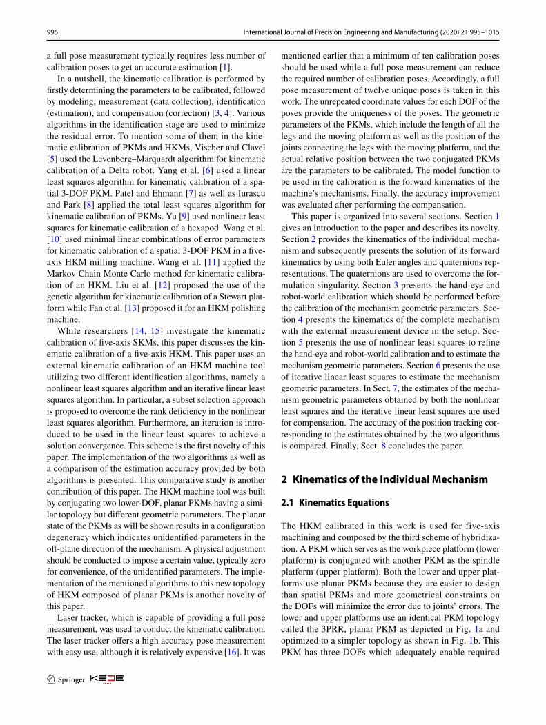
general motion consisting of translation in X-axis, trans-lation in Y-axis, and rotation about the Z-axis, where the three axes are orthogonal and follow the right-hand rule. It consists of a fixed base, three legs, a moving platform, and several joints. The joints used in an order starting from the fixed base are prismatic (P) joints, revolute (R) joints which connect the sliders with the legs, and other revolute (R) joints which connect the legs with the moving platform. Therefore, the mechanism is called the 3PRR PKM. The prismatic joints are actuated, have translation along X-axis, and are implemented by using sliders moving along the base through guideway. The use of the sliders creates more workspace and enables the moving platform to move upward and downward as well as to tilt. The actuation is provided by linear motors which give more accuracy compared with pneumatic/hydraulic pistons and lead screws.

In this proposed mechanism, three legs are required to con-strain the mechanism fully. Furthermore, two neighboring legs are maintained in a crossing configuration to avoid singularity as well as maximize the useful workspace and the stiffness of the mechanism. Point (x, y) in the moving platform is used to evaluate the general motion of the moving platform. Any other

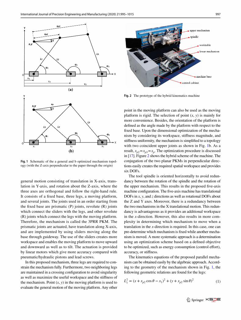
point in the moving platform can also be used as the moving platform is rigid. The selection of point (x, y) is mainly for more convenience. Besides, the orientation of the platform is defined as the angle made by the platform with respect to the fixed base. Upon the dimensional optimization of the mecha-nism by considering its workspace, stiffness magnitude, and stiffness uniformity, the mechanism is simplified to a topology with two coincident upper joints as shown in Fig. 1b. As a result, xp2 = xp3 = xp. The optimization procedure is discussed in [17]. Figure 2 shows the hybrid scheme of the machine. The conjugation of the two planar PKMs in perpendicular direc-tions easily creates the required spatial workspace and provides six DOFs.

The tool spindle is oriented horizontally to avoid redun-dancy between the rotation of the spindle and the rotation of the upper mechanism. This results in the proposed five-axis machine configuration. The five-axis machine has translational DOFs in x, y, and z directions as well as rotational DOFs about the Z and Y axes. Moreover, there is a redundancy between the two mechanisms in the X translational motion. This redun-dancy is advantageous as it provides an additional workspace in the x-direction. However, this also results in more com-plexity in determining which mechanism to move when a translation in the x-direction is required. In this case, one can pre-determine which mechanism is fixed while another mecha-nism is moved. A more systematic approach is a determination using an optimization scheme based on a defined objective to be optimized, such as energy consumption (control effort), accuracy, or stiffness.

The kinematics equations of the proposed parallel mecha-nism can be obtained easily by the algebraic approach. Accord-ing to the geometry of the mechanism shown in Fig. 1, the following geometric relations are found for the legs:

(1)L21= (x + xp2 cos � − x1)

2 + (y + xp2 sin �)2

Fig. 1 Schematic of the a general and b optimized mechanism topol-ogy (with the Z-axis perpendicular to the paper through the origin)

Fig. 2 The prototype of the hybrid kinematics machine


1 3

In this paper, only the forward kinematics of the mechanism is discussed as it is required in the kinematic calibration.

The kinematics of the mechanism has the following constraints:

where ymax and xmax are the vertical and horizontal limits of the machine volume having the numerical values of 1200 mm and 1700 mm, respectively. Those constraints indicate that the mechanism should always be inside the specified machine volume, the sliders should not interfere with each other, and two adjacent legs must always be cross-ing each other.

2.2 Forward Kinematics with Known θ

The complete forward kinematics of the mechanism at hand which includes the determination of the angle θ can be seen in [17]. In this paper, only the determination of x and y given the angle θ is presented for the kinematic calibration pur-pose. In the case of a known θ, the value of x and y can be obtained through a more straightforward derivation. Let us rearrange the kinematics Eqs. (1), (2), and (3) in the follow-ing set of equations:

Collecting x and y in (5)–(7) in the left-hand sides yields:

(2)L22= (x − x2)

2 + (y)2

(3)L23= (x + xp3 cos � − x3)

2 + (y + xp3 sin �)2

(4)

0 ≤ L1 ≤ ymax

0 ≤ L2 ≤ ymax

0 ≤ L3 ≤ ymax

0 ≤ xp2 ≤ xp3 ≤ xmax

L1 + L2 − xp2 ≤ xmax

L1 + L3 − xp2 + xp3 ≤ xmax

(5)x2 + y2 + 2xxp2 cos � + 2yxp2 sin �

− 2x1x − 2x1xp2 cos � = L21− x2

1− x2

p2= c1

(6)x2 + y2 − 2x2x = L22− x2

2= c2

(7)x2 + y2 + 2xxp3 cos � + 2yxp3 sin �

− 2x3x − 2x3xp3 cos � = L23− x2

3− x2

p3= c3

(8)x2 − (2x1 + 2xp2 cos �)x + y2 + (2xp2 sin �)y

= 2x1xp2 cos � + L21− x2

1− x2

p2= c4

Furthermore, subtracting (9) from (8) and (10) yields a more compact set of equations as follows:

where

Equations (11) and (12) have to be solved simultaneously as x and y exist in both of the equations. The solution is given by:

2.3 Forward Kinematics Using Quaternion

Observing the solution of the forward kinematics given in (13) and (14), we realize that division by zero occurs when θ = 0 and therefore b = 0. In this situation, x still can be solved by using (13) by converting zero θ to a minimal value near (above or under) zero. The effect of the closeness of θ to zero can be evaluated by observing the value of the solution, i.e. x and y, as well as the corresponding links’ dimension if we apply the solution. The latter shows a more obvious effect. After scanning some values of θ close to zero, it is shown that θ should not be larger than 1 × 10−5. This will give an accurate solution to four decimal places. Using a closer value of θ to zero increases further the accuracy. Table 1 shows the values of the link lengths corresponding

(9)x2 − (2x2)x + y2 = L22− x2

2= c2

(10)x2 − (2x3 + 2xp3 cos �)x + y2 + (2xp3 sin �)y

= 2x3xp3 cos � + L23− x2

3− x2

p3= c5

(11)(−2x1)x + (2xp2 cos �)x + (2x2)x

+ (2xp2 sin �)y = ax + by = c4 − c2 = c

(12)x2 − (2x2)x + y2 = L22− x2

2= c2

a = −2x1 + 2x2 + 2xp2 cos �

b = 2xp2 sin �

c = c4 − c2

d = −2x3 + 2x2 + 2xp3 cos �

e = 2xp3 sin �

f = c5 − c2

(13)x =

(f −

ec

b

d −ea

b

)

(14)y =c − ax

b


1 3

to different values of θ near zero, given the expected actual values of L1= 600 mm, L2 = 600 mm, and L3 = 750 mm.

On the other hand, division by zero in (14) is very sensi-tive. Even a minimal value of θ replacing an exact zero θ leads to a significant error in the solution, i.e. the value of y. Therefore, (14) cannot be used to solve for y in the case of zero tilting angle of the moving platform. In such a case, either one of the following two ways can be used. First, using an iterative technique by spanning over possible values of y and checking with the inverse kinematics. For any set of x, y, and θ, it should be observed if it retrieves a known set of x1, x2, and x3. However, the accuracy of this technique is affected by the interval of y used in the iteration. Besides, this technique is computationally intensive. Second, solving the forward kinematics by using quaternion. The reason for using the quaternion is because a formulation singularity causes this problem due to the use of Euler angle θ. There-fore, avoiding using the Euler angle by using the quaternion will avoid the formulation singularity.

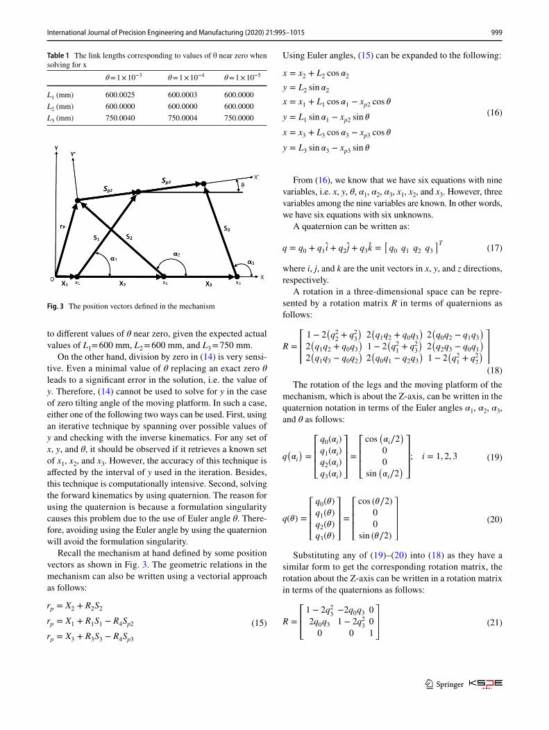
Recall the mechanism at hand defined by some position vectors as shown in Fig. 3. The geometric relations in the mechanism can also be written using a vectorial approach as follows:

(15)

rp = X2 + R2S2

rp = X1 + R1S1 − R4Sp2

rp = X3 + R3S3 − R4Sp3

Using Euler angles, (15) can be expanded to the following:

From (16), we know that we have six equations with nine variables, i.e. x, y, θ, α1, α2, α3, x1, x2, and x3. However, three variables among the nine variables are known. In other words, we have six equations with six unknowns.

A quaternion can be written as:

where i, j, and k are the unit vectors in x, y, and z directions, respectively.

A rotation in a three-dimensional space can be repre-sented by a rotation matrix R in terms of quaternions as follows:

The rotation of the legs and the moving platform of the mechanism, which is about the Z-axis, can be written in the quaternion notation in terms of the Euler angles α1, α2, α3, and θ as follows:

Substituting any of (19)–(20) into (18) as they have a similar form to get the corresponding rotation matrix, the rotation about the Z-axis can be written in a rotation matrix in terms of the quaternions as follows:

(16)

x = x2 + L2 cos �2

y = L2 sin �2

x = x1 + L1 cos �1 − xp2 cos �

y = L1 sin �1 − xp2 sin �

x = x3 + L3 cos �3 − xp3 cos �

y = L3 sin �3 − xp3 sin �

(17)q = q0 + q1 i + q2 j + q3k =[q0 q1 q2 q3

]T

(18)

R =

⎡⎢⎢⎣

1 − 2�q22+ q2

3

�2�q1q2 + q0q3

�2�q0q2 − q1q3

�2�q1q2 + q0q3

�1 − 2

�q21+ q2

3

�2�q2q3 − q0q1

�2�q1q3 − q0q2

�2�q0q1 − q2q3

�1 − 2

�q21+ q2

2

�⎤⎥⎥⎦

(19)q��i

�=

⎡⎢⎢⎢⎣

q0(�i)

q1(�i)

q2(�i)

q3(�i)

⎤⎥⎥⎥⎦=

⎡⎢⎢⎢⎣

cos��i∕2

�0

0

sin��i∕2

�

⎤⎥⎥⎥⎦; i = 1, 2, 3

(20)q(�) =

⎡⎢⎢⎢⎣

q0(�)

q1(�)

q2(�)

q3(�)

⎤⎥⎥⎥⎦=

⎡⎢⎢⎢⎣

cos (�∕2)

0

0

sin (�∕2)

⎤⎥⎥⎥⎦

(21)R =

⎡⎢⎢⎣

1 − 2q23−2q0q3 0

2q0q3 1 − 2q230

0 0 1

⎤⎥⎥⎦

Table 1 The link lengths corresponding to values of θ near zero when solving for x

θ = 1 × 10−3 θ = 1 × 10−4 θ = 1 × 10−5

L1 (mm) 600.0025 600.0003 600.0000L2 (mm) 600.0000 600.0000 600.0000L3 (mm) 750.0040 750.0004 750.0000

Fig. 3 The position vectors defined in the mechanism


1 3

Now we can express the geometric relations (16) by utilizing the rotation matrices in terms of the quaternions (21):

Furthermore, we can write the unit norm constraints of the quaternions as follows:

Since in this case:

then we can rewrite (28)–(29) as follows:

To this point, we can see that we have ten equations with thirteen variables, i.e. x, y, q0(α1), q3(α1), q0(α2), q3(α2), q0(α3), q3(α3), q0(θ), q3(θ), x1, x2, and x3. However, three variables among the 13 variables are known. In other words, we have ten equations with ten unknowns.

For ease, x can be computed using (13). When θ is zero, we can replace it with a small value near zero to accurately compute x. Once θ and x are obtained, we can use any pair of (22)–(23), (24)–(25), or (26) – (27). Using (22)–(23) is easier since we do not involve q3(θ) for which we need to convert θ to get q3(θ). From (22), we have:

Substituting (33) into (31), we obtain the following:

(22)x = x2 + L2(1 − 2q3(�2)2)

(23)y = 2L2q0(�2)q3(�2)

(24)x = x1 + L1(1 − 2q3(�1)2) − xp2(1 − 2q3(�)

2)

(25)y = 2L1q0(�1)q3(�1) − 2xp2q0(�)q3(�)

(26)x = x3 + L3(1 − 2q3(�3)2) − xp3(1 − 2q3(�)

2)

(27)y = 2L3q0(�3)q3(�3) − 2xp3q0(�)q3(�)

(28)q0(�i)2 + q1(�i)

2 + q2(�i)2 + q3(�i)

2 = 1; i = 1, 2, 3

(29)q0(�)2 + q1(�)

2 + q2(�)2 + q3(�)

2 = 1

(30)q1(�1) = q2(�1) = q1(�2) = q2(�2)

= q1(�3) = q2(�3) = q1(�) = q2(�) = 0

(31)q0(�i)2 + q3(�i)

2 = 1; i = 1, 2, 3

(32)q0(�)2 + q3(�)

2 = 1

(33)q3(�2) =

√(1

2−

x − x2

2L2

)

(34)q0(�2) =

√(1

2+

x − x2

2L2

)

Now we can get y in terms of the knowns by substituting (34) into (23):

It is worth mentioning that (35) applies for all values of θ, not only for θ equal or close to zero. Therefore, it is more practical to use (35) instead of (14) to compute y for all cases.

3 Hand‑Eye and Robot‑World Calibration

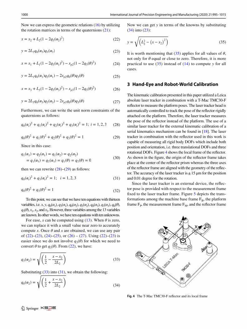
The kinematic calibration presented in this paper utilized a Leica absolute laser tracker in combination with a T-Mac TMC30-F reflector to measure the platform poses. The laser tracker head is automatically controlled to track the pose of the reflector rigidly attached on the platform. Therefore, the laser tracker measures the pose of the reflector instead of the platform. The use of a similar laser tracker for the external kinematic calibration of a serial kinematics mechanism can be found in [18]. The laser tracker in combination with the reflector used in this work is capable of measuring all rigid body DOFs which include both position and orientation, i.e. three translational DOFs and three rotational DOFs. Figure 4 shows the local frame of the reflector. As shown in the figure, the origin of the reflector frame takes place at the center of the reflector prism whereas the three axes of the reflector frame are aligned with the geometry of the reflec-tor. The accuracy of the laser tracker is ± 15 μm for the position and 0.01 degree for the rotation.

Since the laser tracker is an external device, the reflec-tor pose is provided with respect to the measurement frame fixed to the laser tracker frame. Figure 5 depicts the trans-formations among the machine base frame FB, the platform frame FP, the measurement frame FM, and the reflector frame

(35)y =

√(L22−(x − x2

)2)

Fig. 4 The T-Mac TMC30-F reflector and its local frame


1 3

Fr. T1 is the transformation from the machine base frame to the platform. This is given by the forward kinematics of the mechanism. T2 is the transformation from the measure-ment frame to the reflector frame. X1 is the transformation from the reflector frame to the platform, whereas X2 is the transformation from the measurement frame to the machine base frame. The platform or end-effector is commonly called a hand whereas the reflector is called an eye. A calibration to estimate the transformation X1 is accordingly called the hand-eye calibration. The measurement frame is also com-monly called the world frame and consequently a calibration to estimate the transformation X2 is usually called the robot-world calibration. Since the laser tracker at hand is capable of providing the six-DOF pose of the reflector, T2 is wholly known. Unfortunately, X1 and X2 are unknown. As a result, they should be estimated before calibrating the mechanism.

To solve for X1 and X2, at least three different poses of the mechanism should be measured and T1 should be available. In this case, T1 is obtained based on the nominal values of the mechanism geometry. Hence, the estimation of X1 and X2 assumes that the nominal values of the mechanism geometry are good enough. These nominal values are to be calibrated later based on the obtained X1 and X2. The estimation of X1 and X2 can be classified into two broad categories: separable (sequential) and simultaneous techniques. The former tech-niques include [19–23] whereas the latter techniques include [24–31]. In the former techniques, X1 is first obtained and subsequently, X2 is computed based on the obtained X1. This approach is more straightforward but gives a less precise solution. On the other hand, the latter techniques estimate both X1 and X2 simultaneously. In this work, the former approach is applied only to obtain the initial values for the next algorithm proposed to refine the solution.

Let T1, T2, X1, and X2 be homogeneous transformation matrices which contain both rotation and translation com-ponents. The estimation of X1 can be derived based on the following relation among the transformation matrices:

For a pair of mechanism poses as illustrated in Fig. 6, we have the following:

It can be observed from Fig. 6 that X1 and X2 are constant, whereas T1 and T2 change with the mechanism pose.

Upon manipulating (37a) and (37b), we have:

where

Notice that A and B are homogeneous transformation matrices. RA and RB are rotation matrices whereas tA and tB are position vectors. Equation (38), commonly known as AX = XB problem, is the hand-eye calibration problem.

A separable closed-form hand-eye calibration following [19] is employed here. Instead of describing the hand-eye calibration procedure in a derivation format, the proce-dure is described briefly here in a sequential manner as the following:

Step 1 Find the transformation T1 of two different poses. This is obtained by the forward kinematics of the mecha-nism using the nominal values of the mechanism geom-etry, namely L1, L2, L3, xp2, and xp3.

(36)T2X1 = X2T1

(37a)T21X1 = X2T11

(37b)T22X1 = X2T12

(38)AX1 = X1B

(39)A = T−122T21 =

[RA tA0 1

]

(40)B = T−112T11 =

[RB tB0 1

]

Fig. 5 Transformations T1, T2, X1, and X2 Fig. 6 Transformations in a pair of mechanism poses


1 3

Step 2 Find the transformation T2 of the two poses. This is given directly by the measurement of the full pose of the reflector by using the laser tracker. In this work, the measurement of the reflector orientation is provided in quaternions.Step 3 Compute the matrices A and B for the two poses by using (39) and (40).Step 4 Convert the rotation matrices RA and RB into an axis-angle representation defined by a rotation angle α and a rotation axis (n1, n2, n3).Step 5 Define PA and PB as follows:

Step 6 Define υ and S as follows:

Step 7 We have the following linear system:

With only a pair of poses, this linear system is singular. Therefore, at least two pairs of poses, i.e. three different poses, are required. Perform Step 1 to Step 7 for all n poses and accordingly stack (45) from all pairs of poses to compose the following overdetermined system:

Solve for PX1 by using linear least squares:

(41)PA = 2 sin

�𝛼(A)

2

�⎡⎢⎢⎣

n(A)

1

n(A)

2

n(A)

3

⎤⎥⎥⎦; 0 ≤ 𝛼

(A)≤ 𝜋

(42)PB = 2 sin

�𝛼(B)

2

�⎡⎢⎢⎣

n(B)

1

n(B)

2

n(B)

3

⎤⎥⎥⎦; 0 ≤ 𝛼

(B)≤ 𝜋

(43)𝜐 =

⎡⎢⎢⎣

𝜐x

𝜐y

𝜐z

⎤⎥⎥⎦= PA + PB

(44)S = skew(�) =

⎡⎢⎢⎣

0 −�z �y

�z 0 −�x−�y �x 0

⎤⎥⎥⎦

(45)S PX1= PA − PB

(46)⌢

S PX1=

⎡⎢⎢⎢⎣

S1S2⋮

Sn

⎤⎥⎥⎥⎦PX1

= b =

⎡⎢⎢⎢⎣

�PA − PB

�1�

PA − PB

�2

⋮�PA − PB

�n

⎤⎥⎥⎥⎦

(47)PX1=

(⌢

S

T⌢

S

)−1⌢

S

T

b

Step 8 Compute PX1 as follows:

Step 9 Convert PX1 to the rotation matrix of the transfor-

mation X1, namely RX1:

where I is an identity matrix whereas skew(PX1

) is a

skew-symmetric matrix defined in a similar fashion to (44). To this point, we solve for the rotation matrix of the transformation X1.Step 10: Define a linear system involving the translation vector of the transformation X1, namely tX1, as follows:

Solve the linear system (50) by using linear least squares:

Equations (50) and (51) hold in general for three-dimen-sional Euclidean space. Since the mechanism at hand is planar, the dimensions of (50) and (51) should be reduced to a two-dimensional Euclidean space. Having the mecha-nism on the XY plane, the elements corresponding to the Z-axis in (50) and (51) should be suppressed. If it is not sup-pressed and accordingly x, y, and z elements of tX1 are all to be solved, the system will be rank deficient. This indicates a configuration degeneracy. Physically, this means that there is no reference in the z-direction to which the z element of tX1 should be defined. As a result, an infinite number of pos-sible values of z exist.

Equations (49) and (51) completely define the transforma-tion matrix X1:

where, in the case of planar mechanism working on the XY plane:

(48)PX1

=2 PX1√

1 +‖‖‖PX1

‖‖‖2

(49)RX1

=

⎛⎜⎜⎜⎝1 −

��PX1

��2

2

⎞⎟⎟⎟⎠I +

1

2

�PX1

PT

X1

+

�4 −

��PX1

��2

skew�PX1

��

(50)GtX1=(RB − I

)tX1

= d = RX1tA − tB

(51)tX1=(GTG

)−1GTd

(52)X1 =

[RX1

tX1

0 1

]

(53)tX1=

⎡⎢⎢⎣

tX1(x)

tX1(y)

0

⎤⎥⎥⎦


1 3

Equation (53) also implies that the zero coordinate of the Z-axis is aligned with the reflector.

After the hand-eye transformation X1 has been estimated, the robot-world transformation X2 can be easily estimated by rearranging (36):

Using n different mechanism poses in the measurement, we accordingly have n different T1 and T2. As a result, there will be n different X2. To obtain a single X2, which is expected to be constant, we average the elements of T1 and T2 in an element-wise manner to get an averaged, constant X2.

It is worth mentioning that the selected poses should be completely different from each other in all coordinates in order to get the best estimates. In this case, the x, y, and θ values should be completely different among the poses. In this work, twelve experimental measurement data was care-fully taken in which the x, y, and θ values of the poses are entirely different.

4 Kinematics of the Combined Mechanism with the External Measurement Device

The pose measurement is always provided with respect to the measurement frame. Since the kinematic calibration uses an external pose-measurement device, an extended kinematic model should be established to include the hand-eye and robot-world transformations as described earlier. A homogeneous transformation is very convenient to be used

(54)X2 = T2X1T−11

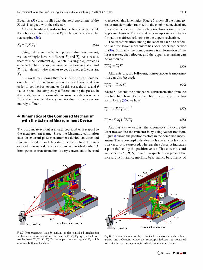
to represent this kinematics. Figure 7 shows all the homoge-neous transformation matrices in the combined mechanism. For convenience, a similar matrix notation is used for the upper mechanism. The asterisk superscripts indicate trans-formation matrices belonging to the upper mechanism.

The transformation among the laser tracker, the reflec-tor, and the lower mechanism has been described earlier in (36). Similarly, the homogeneous transformation of the laser tracker, the reflector, and the upper mechanism can be written as:

Alternatively, the following homogeneous transforma-tion can also be used:

where X0 denotes the homogeneous transformation from the machine base frame to the base frame of the upper mecha-nism. Using (56), we have:

Another way to express the kinematics involving the laser tracker and the reflector is by using vector notation. Figure 8 shows the position vectors in the combined mech-anism. The superscript indicates the frame in which a posi-tion vector r is expressed, whereas the subscript indicates a point defined by the position vector. The subscripts and superscripts M, B, O, P, and r respectively represent the measurement frame, machine base frame, base frame of

(55)T∗2X∗1= X∗

2T∗1

(56)T∗2X∗1= X2X0T

∗1

(57)T∗2= X2X0T

∗1

(X∗1

)−1

(58)T∗1=(X2X0

)−1T∗2X∗1

Fig. 7 Homogeneous transformations in the combined mechanism with a laser tracker and reflectors, namely T1, T2, X1, X2 (for the lower mechanism), T∗

1,T

∗2,X

∗1,X

∗2 (for the upper mechanism), and X0 which

connects both mechanisms

Fig. 8 Position vectors in the combined mechanism with a laser tracker and reflectors, where the subscripts indicate the points of interest whereas the superscripts indicate the reference frames


1 3

the upper mechanism, platform frame, and reflector frame. For example, a notation rM

B denotes the position vector of

the machine base frame origin B with respect to the meas-urement frame M.

The additional subscripts L and U indicate the lower and upper mechanism, respectively. The transformation between frames may involve a rotation matrix R which represents the rotational transformation between two frames. Similarly, a notation RM

B , as an example, denotes

the rotation matrix from the machine base frame B to the measurement frame M.

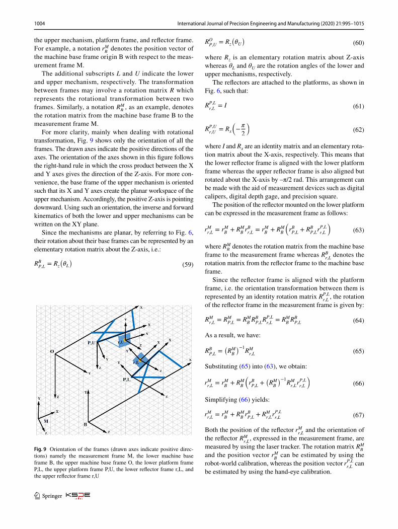
For more clarity, mainly when dealing with rotational transformation, Fig. 9 shows only the orientation of all the frames. The drawn axes indicate the positive directions of the axes. The orientation of the axes shown in this figure follows the right-hand rule in which the cross product between the X and Y axes gives the direction of the Z-axis. For more con-venience, the base frame of the upper mechanism is oriented such that its X and Y axes create the planar workspace of the upper mechanism. Accordingly, the positive Z-axis is pointing downward. Using such an orientation, the inverse and forward kinematics of both the lower and upper mechanisms can be written on the XY plane.

Since the mechanisms are planar, by referring to Fig. 6, their rotation about their base frames can be represented by an elementary rotation matrix about the Z-axis, i.e.:

(59)RBP,L

= Rz

(�L

)

where Rz is an elementary rotation matrix about Z-axis whereas θL and θU are the rotation angles of the lower and upper mechanisms, respectively.

The reflectors are attached to the platforms, as shown in Fig. 6, such that:

where I and Rx are an identity matrix and an elementary rota-tion matrix about the X-axis, respectively. This means that the lower reflector frame is aligned with the lower platform frame whereas the upper reflector frame is also aligned but rotated about the X-axis by –π/2 rad. This arrangement can be made with the aid of measurement devices such as digital calipers, digital depth gage, and precision square.

The position of the reflector mounted on the lower platform can be expressed in the measurement frame as follows:

where RMB

denotes the rotation matrix from the machine base frame to the measurement frame whereas RB

r,L denotes the

rotation matrix from the reflector frame to the machine base frame.

Since the reflector frame is aligned with the platform frame, i.e. the orientation transformation between them is represented by an identity rotation matrix RP,L

r,L , the rotation

of the reflector frame in the measurement frame is given by:

As a result, we have:

Substituting (65) into (63), we obtain:

Simplifying (66) yields:

Both the position of the reflector rMr,L

and the orientation of the reflector RM

r,L , expressed in the measurement frame, are

measured by using the laser tracker. The rotation matrix RMB

and the position vector rM

B can be estimated by using the

robot-world calibration, whereas the position vector rP,Lr,L

can be estimated by using the hand-eye calibration.

(60)ROP,U

= Rz

(�U

)

(61)RP,L

r,L= I

(62)RP,U

r,U= Rx

(−�

2

)

(63)rMr,L

= rMB+ RM

BrBr,L

= rMB+ RM

B

(rBP,L

+ RBP,L

rP,L

r,L

)

(64)RMr,L

= RMP,L

= RMBRBP,L

RP,L

r,L= RM

BRBP,L

(65)RBP,L

=(RMB

)−1RMr,L

(66)rMr,L

= rMB+ RM

B

(rBP,L

+(RMB

)−1RMr,LrP,L

r,L

)

(67)rMr,L

= rMB+ RM

BrBP,L

+ RMr,LrP,L

r,L

Fig. 9 Orientation of the frames (drawn axes indicate positive direc-tions) namely the measurement frame M, the lower machine base frame B, the upper machine base frame O, the lower platform frame P,L, the upper platform frame P,U, the lower reflector frame r,L, and the upper reflector frame r,U


1 3

The position of the platform end-effector in the base frame rB

P,L is given by the forward kinematics, i.e.:

where f1 and f2 are the forward kinematics equations and PL contains all the geometric parameters of the lower mechanism.

For convenience, the Z-axis of the machine base frame is assumed to be aligned with the Z-axis of the reflector frame. In other words, the z coordinate of the reflector frame origin with respect to the machine base frame is zero:

Similarly, the position of the reflector mounted on the upper platform can be expressed in the measurement frame as follows:

The rotation of the reflector frame in the measurement frame, which is measured by using the laser tracker, can be written as:

Solving for ROP,U

from (71) yields:

Because we have (62), then:

Substituting (73) into (70), we obtain:

In fact, both the position of the reflector rMr,U

and the ori-entation of the reflector RM

r,U , expressed in the measurement

frame, are measured by using the laser tracker. The rota-tion matrix RM

O and the position vector rM

O can be estimated

by using the robot-world calibration, whereas the position vector rP,U

r,U can be estimated by using the hand-eye calibra-

tion. The position of the platform end-effector in the base

(68)rBP,L

=

⎡⎢⎢⎣

xLyLzL

⎤⎥⎥⎦=

⎡⎢⎢⎣

f1(x1, x2, x3,PL)

f2(x1, x2, x3,PL)

0

⎤⎥⎥⎦

(69)rP,L

r,L=

⎡⎢⎢⎣

xr,Lyr,Lzr,L

⎤⎥⎥⎦=

⎡⎢⎢⎣

xr,Lyr,L0

⎤⎥⎥⎦

(70)rMr,U

= rMO+ RM

OrOr,U

= rMO+ RM

O

(rOP,U

+ ROP,U

rP,U

r,U

)

(71)RMr,U

= RMOROP,U

RP,U

r,U

(72)ROP,U

=(RMO

)−1RMr,U

(RP,U

r,U

)−1

(73)ROP,U

=(RMO

)−1RMr,U

(Rx

(−�

2

))−1

(74)

rMr,U

= rMO+ RM

OrOr,U

= rMO+ RM

O

(rOP,U

+

((RMO

)−1RMr,U

(Rx

(−�

2

))−1)rP,U

r,U

)

frame of the upper mechanism rOP,U

is given by the forward kinematics, i.e.:

where f1 and f2 are the forward kinematics equations and PU contains all the geometric parameters of the upper mechanism.

The transformation from the machine base frame B to the base frame of the upper mechanism O can be obtained from the following relations:

From (76) and (77), we obtain:

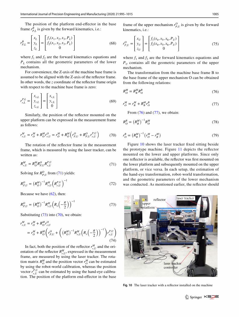
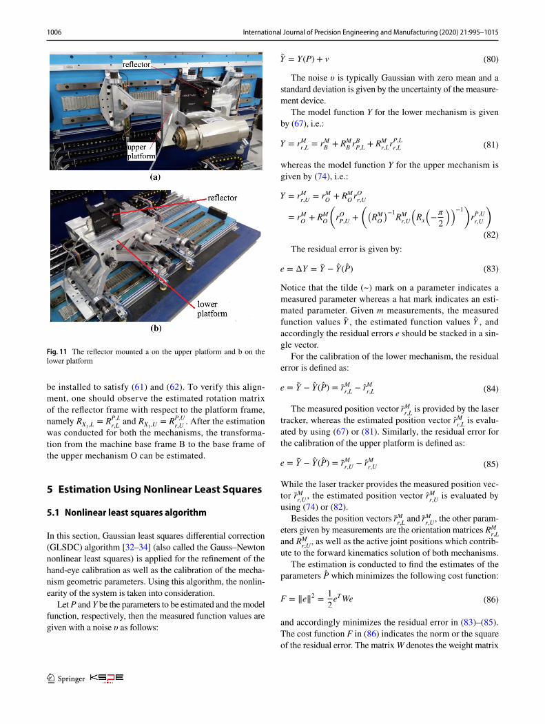
Figure 10 shows the laser tracker fixed sitting beside the prototype machine. Figure 11 depicts the reflector mounted on the lower and upper platforms. Since only one reflector is available, the reflector was first mounted on the lower platform and subsequently mounted on the upper platform, or vice versa. In each setup, the estimation of the hand-eye transformation, robot-world transformation, and the geometric parameters of the lower mechanism was conducted. As mentioned earlier, the reflector should

(75)rOP,U

=

⎡⎢⎢⎣

xUyUzU

⎤⎥⎥⎦=

⎡⎢⎢⎣

f1(x4, x5, x6,PU)

f2(x4, x5, x6,PU)

0

⎤⎥⎥⎦

(76)RMO= RM

BRBO

(77)rMO= rM

B+ RM

BrBO

(78)RBO=(RMB

)−1RMO

(79)rBO=(RMB

)−1(rMO− rM

B

)

Fig. 10 The laser tracker with a reflector installed on the machine


1 3

be installed to satisfy (61) and (62). To verify this align-ment, one should observe the estimated rotation matrix of the reflector frame with respect to the platform frame, namely RX1,L

= RP,L

r,L and RX1,U

= RP,U

r,U . After the estimation

was conducted for both the mechanisms, the transforma-tion from the machine base frame B to the base frame of the upper mechanism O can be estimated.

5 Estimation Using Nonlinear Least Squares

5.1 Nonlinear least squares algorithm

In this section, Gaussian least squares differential correction (GLSDC) algorithm [32–34] (also called the Gauss–Newton nonlinear least squares) is applied for the refinement of the hand-eye calibration as well as the calibration of the mecha-nism geometric parameters. Using this algorithm, the nonlin-earity of the system is taken into consideration.

Let P and Y be the parameters to be estimated and the model function, respectively, then the measured function values are given with a noise υ as follows:

The noise υ is typically Gaussian with zero mean and a standard deviation is given by the uncertainty of the measure-ment device.

The model function Y for the lower mechanism is given by (67), i.e.:

whereas the model function Y for the upper mechanism is given by (74), i.e.:

The residual error is given by:

Notice that the tilde (~) mark on a parameter indicates a measured parameter whereas a hat mark indicates an esti-mated parameter. Given m measurements, the measured function values Y , the estimated function values Y , and accordingly the residual errors e should be stacked in a sin-gle vector.

For the calibration of the lower mechanism, the residual error is defined as:

The measured position vector rMr,L

is provided by the laser tracker, whereas the estimated position vector rM

r,L is evalu-

ated by using (67) or (81). Similarly, the residual error for the calibration of the upper platform is defined as:

While the laser tracker provides the measured position vec-tor rM

r,U , the estimated position vector rM

r,U is evaluated by

using (74) or (82).Besides the position vectors rM

r,L and rM

r,U , the other param-

eters given by measurements are the orientation matrices RMr,L

and RM

r,U , as well as the active joint positions which contrib-

ute to the forward kinematics solution of both mechanisms.The estimation is conducted to find the estimates of the

parameters P which minimizes the following cost function:

and accordingly minimizes the residual error in (83)–(85). The cost function F in (86) indicates the norm or the square of the residual error. The matrix W denotes the weight matrix

(80)Y = Y(P) + v

(81)Y = rMr,L

= rMB+ RM

BrBP,L

+ RMr,LrP,L

r,L

(82)

Y = rMr,U

= rMO+ RM

OrOr,U

= rMO+ RM

O

(rOP,U

+

((RMO

)−1RMr,U

(Rx

(−�

2

))−1)rP,U

r,U

)

(83)e = ΔY = Y − Y(P)

(84)e = Y − Y(P) = rMr,L

− rMr,L

(85)e = Y − Y(P) = rMr,U

− rMr,U

(86)F = ‖e‖2 = 1

2eTWe

Fig. 11 The reflector mounted a on the upper platform and b on the lower platform


1 3

which is, in this work, chosen to be an identity matrix. Using GLSDC, the parameter estimates are computed iteratively as follows:

where

and the subscript k indicates the k-th iteration.A modification to (88) called the Levenberg–Marquardt

algorithm (also called the damped least squares) had been proposed to speed up the convergence in the case of initial values far from the “true” values. Since the initial val-ues assigned in this work are considered close enough to the “true” values, the GLSDC is sufficient to give a fast convergence.

The Jacobian matrix H is obtained by differentiating the model function with respect to the estimated parameters:

where Yx, Yy, and Yz denote the x, y, and z components of the model function Y.

Given m measurements, the Jacobian matrix H should be stacked as follows:

The squared system Jacobian matrix in each iteration is the inverted part in (88), i.e.:

The matrix J should have a full rank in order to give a trusted solution. This full rank indicates that all the parameters are independent and therefore fully identified. In other words, a rank deficiency by n indicates that n parameters are dependent and therefore unidentified. The determination of the unidentified parameters can be done mathematically or through knowledge on the parameter dependency of the physical system. In a system with a rank deficiency, the dependent parameters should be elimi-nated until a full-rank system is obtained. In such a case, the nominal parameter values can be used. The dependent parameters can be estimated in the next step employing the estimates of the independent parameters having been obtained previously. This is commonly called the subset

(87)Xk+1 = Xk + Δx

(88)Δx =(HT

kWHk

)−1HT

kWek

(89)H =�Y

�P=[Hx Hy Hz

]T=[

�Yx

�P

�Yy

�P

�Yz

�P

]T

(90)Hx =

⎡⎢⎢⎢⎣

�Yx1

�P

⋮�Yxm

�P

⎤⎥⎥⎥⎦; Hy =

⎡⎢⎢⎢⎣

�Yy1

�P

⋮�Yym

�P

⎤⎥⎥⎥⎦; Hz =

⎡⎢⎢⎢⎣

�Yz1

�P

⋮�Yzm

�P

⎤⎥⎥⎥⎦

(91)H3mx5 =[Hx Hy Hz

]T

(92)J = HTkWHk

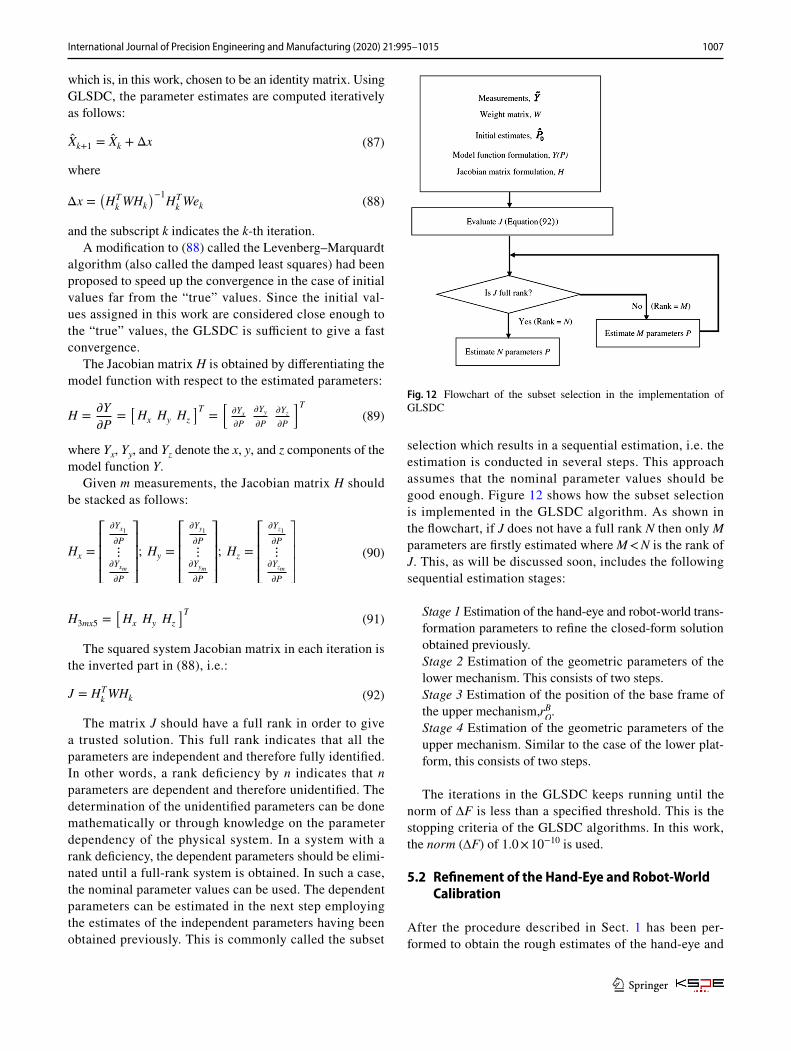
selection which results in a sequential estimation, i.e. the estimation is conducted in several steps. This approach assumes that the nominal parameter values should be good enough. Figure 12 shows how the subset selection is implemented in the GLSDC algorithm. As shown in the flowchart, if J does not have a full rank N then only M parameters are firstly estimated where M < N is the rank of J. This, as will be discussed soon, includes the following sequential estimation stages:

Stage 1 Estimation of the hand-eye and robot-world trans-formation parameters to refine the closed-form solution obtained previously.Stage 2 Estimation of the geometric parameters of the lower mechanism. This consists of two steps.Stage 3 Estimation of the position of the base frame of the upper mechanism,rB

O.

Stage 4 Estimation of the geometric parameters of the upper mechanism. Similar to the case of the lower plat-form, this consists of two steps.

The iterations in the GLSDC keeps running until the norm of ∆F is less than a specified threshold. This is the stopping criteria of the GLSDC algorithms. In this work, the norm (∆F) of 1.0 × 10−10 is used.

5.2 Refinement of the Hand‑Eye and Robot‑World Calibration

After the procedure described in Sect. 1 has been per-formed to obtain the rough estimates of the hand-eye and

Fig. 12 Flowchart of the subset selection in the implementation of GLSDC


1 3

robot-world transformations, a refinement is conducted by using the obtained estimates as initial values in an itera-tive estimation using GLSDC. For the lower mechanism, since the orientation of the reflector frame is aligned with that of the platform frame, the remaining parameters which should be estimated to establish the hand-eye and robot-world transformations are the position and orientation of the machine base frame with respect to the measurement frame, namely rM

B and RM

B , as well as the position of the reflector

with respect to the lower platform frame, namely rP,Lr,L

. As the rotation matrix RM

B is defined in terms of quaternions,

namely q0, q1, q2, and q3, the position vector rMB

is defined by the components xB, yB, and zB, and the position vector rP,L

r,L is defined by the components xr and yr while zr= 0, the

parameters to be estimated are:

Similarly for the upper mechanism, since the orientation of the reflector frame is aligned with that of the platform frame with a rotation of –π/2 about X-axis, the remaining parameters which should be estimated to establish the hand-eye and robot-world transformations are the position and orientation of the machine base frame with respect to the measurement frame, namely rM

O and RM

O , as well as the posi-

tion of the reflector with respect to the lower platform frame, namely rP,U

r,U . As the rotation matrix RM

O is defined in terms

of quaternions, namely q0, q1, q2, and q3, the position vec-tor rM

O is defined by the components xO, yO, and zO, and the

position vector rP,Ur,U

is defined by the components xr and zr while yr= 0, the parameters to be estimated are:

The evaluation of the squared system Jacobian matrix J for both the lower and upper mechanisms shows that its rank is 9 (full rank) and therefore all the parameters in (93) and (94) can be estimated in a single step for each mechanism.

(93)P =[q0 q1 q2 q3 xB yB zB xr yr

]T

(94)P =[q0 q1 q2 q3 xO yO zO xr zr

]T

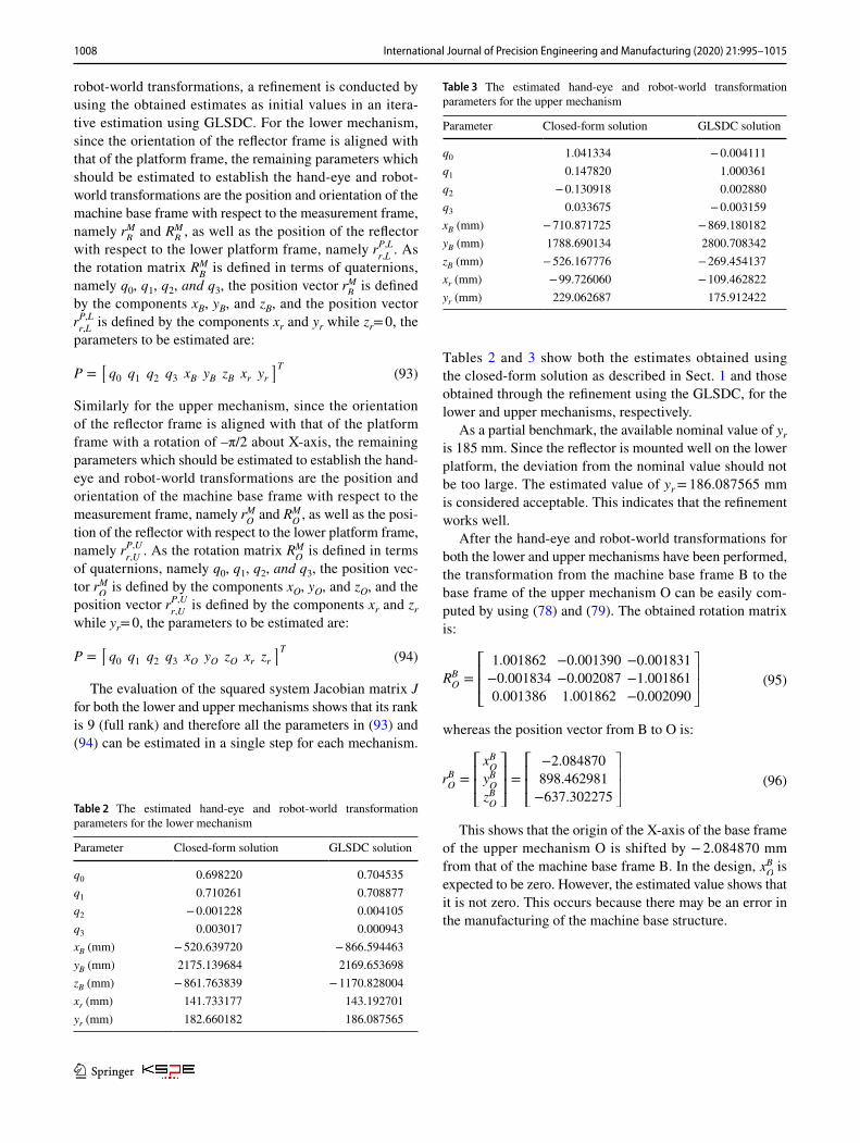
Tables 2 and 3 show both the estimates obtained using the closed-form solution as described in Sect. 1 and those obtained through the refinement using the GLSDC, for the lower and upper mechanisms, respectively.

As a partial benchmark, the available nominal value of yr is 185 mm. Since the reflector is mounted well on the lower platform, the deviation from the nominal value should not be too large. The estimated value of yr = 186.087565 mm is considered acceptable. This indicates that the refinement works well.

After the hand-eye and robot-world transformations for both the lower and upper mechanisms have been performed, the transformation from the machine base frame B to the base frame of the upper mechanism O can be easily com-puted by using (78) and (79). The obtained rotation matrix is:

whereas the position vector from B to O is:

This shows that the origin of the X-axis of the base frame of the upper mechanism O is shifted by − 2.084870 mm from that of the machine base frame B. In the design, xB

O is

expected to be zero. However, the estimated value shows that it is not zero. This occurs because there may be an error in the manufacturing of the machine base structure.

(95)RBO=

⎡⎢⎢⎣

1.001862 −0.001390 −0.001831

−0.001834 −0.002087 −1.001861

0.001386 1.001862 −0.002090

⎤⎥⎥⎦

(96)rBO=

⎡⎢⎢⎣

xBO

yBO

zBO

⎤⎥⎥⎦=

⎡⎢⎢⎣

−2.084870

898.462981

−637.302275

⎤⎥⎥⎦Table 2 The estimated hand-eye and robot-world transformation parameters for the lower mechanism

Parameter Closed-form solution GLSDC solution

q0 0.698220 0.704535q1 0.710261 0.708877q2 − 0.001228 0.004105q3 0.003017 0.000943xB (mm) − 520.639720 − 866.594463yB (mm) 2175.139684 2169.653698zB (mm) − 861.763839 − 1170.828004xr (mm) 141.733177 143.192701yr (mm) 182.660182 186.087565

Table 3 The estimated hand-eye and robot-world transformation parameters for the upper mechanism

Parameter Closed-form solution GLSDC solution

q0 1.041334 − 0.004111q1 0.147820 1.000361q2 − 0.130918 0.002880q3 0.033675 − 0.003159xB (mm) − 710.871725 − 869.180182yB (mm) 1788.690134 2800.708342zB (mm) − 526.167776 − 269.454137xr (mm) − 99.726060 − 109.462822yr (mm) 229.062687 175.912422


1 3

5.3 Estimation of the Mechanism Geometric Parameters

For each mechanism, there are five geometric parameters to be estimated, namely l1, l2, l3, xp2 and xp3. In the case of xp2= xp3= xp, which is the case of the prototype machine, there are four geometric parameters to be estimated, i.e. l1, l2, l3,and xp. Therefore, the parameters to be estimated are:

The observation shows that the squared system Jacobian matrix J gives only a rank of 4 in the case of five parameters to be estimated, i.e. when xp2≠ xp3, and a rank of 3 in the case of four parameters to be estimated, i.e. when xp2= xp3= xp. This is because one of all the geometric parameters to be estimated is dependent on the other four parameters. In other words, all the geometric parameters but one are known then the one parameter remaining can be calculated by using the closed-form geometric relation of the mechanism.

Another approach is to estimate all the geometric param-eters in two steps. In the first step, L2, L3, xp2, and xp3 are estimated. In this step, the nominal value of L1 is used in the estimation iterations. In the second step, the remaining parameter, i.e. L1, is estimated. Although the nominal value of L1 is used in the first step, L1 is subsequently estimated in the second step. Using twelve unique calibration poses for each of the lower and upper mechanisms, the estimates of the geometric parameters of the lower and upper mechanisms along with their nominal values are shown in Tables 4 and 5. The errors are defined as the difference between the esti-mates and the nominal values. It can be observed in Tables 4 and 5 that the estimate of L1 is similar to its nominal value.

(97)P =[L1 L2 L3 xp

]T

This is because the nominal value of L1 is used in the first step and subsequently it is estimated after the other parame-ters have been estimated. In other words, the nominal values of L1 are retrieved in this two-step estimation.

6 Estimation of the Geometric Parameters Using Iterative Linear Least Squares

In this section, a linear error model is used for the kinematic calibration. Accordingly, the closed-form linear least squares estimation can be employed. From the kinematic relations given in (1)–(3), a small perturbation can be introduced to all the parameters which include the geometric parameters P, the active joint positions q, and the platform pose X. This small perturbation which represents a small error is a first-order approximation. Following (1)–(3), the perturbed kinematics can be written by differentiating the kinematics with respect to all parameters:

In a matrix form, (98)–(100) can be written compactly as:

where

(98)

L1�l1 = (x + xp2 cos(�) − x1)

(�x + �xp2 cos(�) − xp2 sin(�)�� − �x1)

+ (y + xp2 sin(�))(�y + �xp2 sin(�) + xp2 cos(�)��)

(99)L2�l2 = (x − x2)(�x − �x2) + y�y

(100)

L3�l3 = (x + xp3 cos(�) − x3)

(�x + �xp3 cos(�) − xp3 sin(�)�� − �x3)

+ (y + xp3 sin(�))(�y + �xp3 sin(�) + xp3 cos(�)��)

(101)Jx�X + Jq�q = Jp�P

(102)

Jx =

⎡⎢⎢⎣

X1 y + xp2 sin(𝜃) X1xp2(cos(𝜃) − sin(𝜃))

(x − x2) y 0

X3 y + xp3 sin(𝜃) X3xp3(cos(𝜃) − sin(𝜃))

⎤⎥⎥⎦

(103)Jq =

⎡⎢⎢⎣

−X1 0 0

0 x2 − x 0

0 0 −X3

⎤⎥⎥⎦

(104)

Jp =

⎡⎢⎢⎣

L1 0 0 −X1(cos 𝜃 + sin 𝜃) 0

0 L2 0 0 0

0 0 L3 0 −X3(cos 𝜃 + sin 𝜃)

⎤⎥⎥⎦

Table 4 The estimates of geometric parameters of the lower mecha-nism (xp2 = xp3 = xp)

Parameter Estimate Nominal value Error

L1 (mm) 486.000000 486.000000 0.000000L2 (mm) 500.985068 500.000000 0.985068L3 (mm) 506.857577 507.000000 − 0.142423xp (mm) 285.866049 285.000000 0.866049

Table 5 The estimates of geometric parameters of the upper mecha-nism (xp2 = xp3 = xp)

Parameter Estimate Nominal value Error

L1 (mm) 600.000000 600 0.000000L2 (mm) 475.001025 475 0.001025L3 (mm) 604.000966 604 0.000966xp (mm) 280.001333 280 0.001333


1 3

Let all the terms in the left-hand side be called A, i.e.:

and B = Jp , then we can rewrite (101) as:

Having m measurements, we can stack (110) into the following overdetermined system:

where

The estimation of �P is aimed at minimizing the fol-lowing cost function:

As the problem is an overdetermined system, a closed-form solution for δp is given by the following linear least squares:

Since (115) denotes the errors in the geometric param-eters, the estimated geometric parameters are given by:

where P and P denote the estimated and nominal values of the geometric parameters, respectively.

Assuming that the measurement is given with respect to the machine base frame, the following is the sequential procedure to implement the linear least squares estimation based on the abovementioned linear error model:

Step 1 Assign the poses to be visited, X.

(105)X1 = x + xp2 cos(𝜃) − x1

(106)X3 = x + xp3 cos(𝜃) − x3

(107)�X =[�x �y ��

]T

(108)�q =[�x1 �x2 �x3

]T

(109)�P =[�L1 �L2 �L3 �xp2 �xp3

]T

(110)A = Jx�X + Jq�q

(111)A = B�P

(112)A = B𝛿P

(113)A =

⎡⎢⎢⎢⎣

A1

A2

⋮

Am

⎤⎥⎥⎥⎦; B =

⎡⎢⎢⎢⎣

B1

B2

⋮

Bm

⎤⎥⎥⎥⎦

(114)F = ‖‖B𝛿p − A‖‖2 = 1

2

(B𝛿p − A

)2

(115)𝛿P =(BT B

)BT A

(116)P = P + 𝛿P

Step 2 Measure the poses, Xmeasured.Step 3 Calculate δX = Xmeasured − X.Step 4 Perform the inverse kinematics to obtain the active joint positions q = f(X,P).Step 5 Measure the active joint positions, qmeasured.Step 6 Calculate δq = qmeasured – q.Step 7 Calculate A(X, �X, q, �q,P) = Jx�X + Jq�q [Eq. (110)].Step 8 Compose the vector B(X,q,P).Step 9 Repeat Step 1 to Step 8 for m measurements. Compose A and B as in (113).Step 10 Check the rank of BT B.Step 11 If BT B has full rank, then compute the linear least squares solution (115). Otherwise, eliminate the dependent parameters either mathematically, such as through SVD, or based on knowledge on the physical system.

In real practice, the measured poses Xmeasured is often given by an external measurement device such as a camera or a laser tracker as in this work. As a result, Xmeasured is given with respect to a measurement frame which is not aligned with the machine base frame. Accordingly, the assigned poses X should be defined with respect to the measurement frame. The values of X with respect to the measurement frame can be derived from (67) or (81) for the lower mechanism and from (74) or (82) for the upper mechanism.

From (67) or (81), we obtain:

In a similar fashion, from (74) or (81) we have:

The sequential procedure to implement the linear least squares estimation based on the linear model when an exter-nal pose measurement device is used can be summarized as follows:

Step 1 Estimate the hand-eye and robot-world transfor-mations.Step 2 Assign X with respect to the machine base frame FB for the lower mechanism and with respect to the base frame of the upper mechanism FO for the upper mecha-nism.Step 3 Measure the reflector position with respect to the measurement frame, namely rM

r,L for the lower mechanism

and rMr,U

for the upper mechanism.Step 4 Calculate Xmeasured by utilizing (117) for the lower mechanism and (118) for the upper mechanism.

(117)XL = rBP,L

=(RMB

)−1(rMr,L

− rMB− RM

r,LrP,L

r,L

)

(118)

XU = rOP,U

=(RMO

)−1(rMr,U

− rMO− RM

r,U

(Rx

(−�

2

))−1

rP,U

r,U

)


1 3

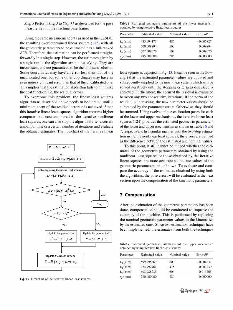
Step 5 Perform Step 3 to Step 11 as described for the pose measurement in the machine base frame.

Using the same measurement data as used in the GLSDC, the resulting overdetermined linear system (112) with all the geometric parameters to be estimated has a full-ranked BT B . Therefore, the estimation can be performed straight-forwardly in a single step. However, the estimates given by a single run of the algorithm are not satisfying. They are inconsistent and not guaranteed to be the optimum solution. Some coordinates may have an error less than that of the uncalibrated one, but some other coordinates may have an even more significant error than that of the uncalibrated one. This implies that the estimation algorithm fails to minimize the cost function, i.e. the residual errors.

To overcome this problem, the linear least squares algorithm as described above needs to be iterated until a minimum norm of the residual errors ε is achieved. Since this iterative linear least squares algorithm requires higher computational cost compared to the iterative nonlinear least squares, one can also stop the algorithm after a certain amount of time or a certain number of iterations and evaluate the obtained estimates. The flowchart of the iterative linear

least squares is depicted in Fig. 13. It can be seen in the flow-chart that the estimated parameter values are updated and subsequently supplied to the new linear system which will be solved iteratively until the stopping criteria as discussed is achieved. Furthermore, the norm of the residual is evaluated between any two consecutive iterations. If the norm of the residual is increasing, the new parameter values should be subtracted by the parameter errors. Otherwise, they should be summed. Using twelve unique calibration poses for each of the lower and upper mechanisms, the iterative linear least squares (124) provides the estimated geometric parameters of the lower and upper mechanisms as shown in Tables 6 and 7, respectively. In a similar manner with the two-step estima-tion using the nonlinear least squares, the errors are defined as the difference between the estimated and nominal values.

To this point, it still cannot be judged whether the esti-mates of the geometric parameters obtained by using the nonlinear least squares or those obtained by the iterative linear squares are more accurate as the true values of the geometric parameters are unknown. To evaluate and com-pare the accuracy of the estimates obtained by using both the algorithms, the pose errors will be evaluated in the next section upon the compensation of the kinematic parameters.

7 Compensation

After the estimation of the geometric parameters has been done, compensation should be conducted to improve the accuracy of the machine. This is performed by replacing the nominal geometric parameter values in the kinematics by the estimated ones. Since two estimation techniques have been implemented, the estimates from both the techniques

Fig. 13 Flowchart of the iterative linear least squares

Table 6 Estimated geometric parameters of the lower mechanism obtained by using iterative linear least squares

Parameter Estimated value Nominal value Error �P

L1 (mm) 485.994173 486 − 0.005827L2 (mm) 500.009894 500 0.009894L3 (mm) 507.009070 507 0.009070xp (mm) 285.000000 285 0.000000

Table 7 Estimated geometric parameters of the upper mechanism obtained by using iterative linear least squares

Parameter Estimated value Nominal value Error �P

L1 (mm) 599.995369 600 − 0.004631L2 (mm) 474.992761 475 − 0.007239L3 (mm) 603.988235 604 − 0.011765xp (mm) 280.000000 280 0.000000


1 3

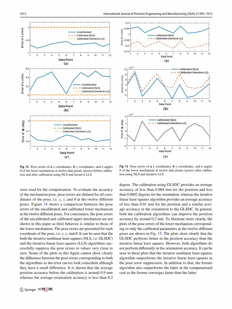
were used for the compensation. To evaluate the accuracy of the mechanism pose, pose errors are defined for all coor-dinates of the pose, i.e. x, y, and θ at the twelve different poses. Figure 14 shows a comparison between the pose errors of the uncalibrated and calibrated lower mechanism at the twelve different poses. For conciseness, the pose errors of the uncalibrated and calibrated upper mechanism are not shown in this paper as their behavior is similar to those of the lower mechanism. The pose errors are presented for each coordinate of the pose, i.e. x, y, and θ. It can be seen that the both the iterative nonlinear least squares (NLS, i.e. GLSDC) and the iterative linear least squares (LLS) algorithms suc-cessfully suppress the pose errors to values very close to zero. Some of the plots in this figure cannot show clearly the difference between the pose errors corresponding to both the algorithms as the error curves look coincident although they have a small difference. It is shown that the average position accuracy before the calibration is around 0.9 mm whereas the average orientation accuracy is less than 0.2

degree. The calibration using GLSDC provides an average accuracy of less than 0.004 mm for the position and less than 0.0002 degrees for the orientation, whereas the iterative linear least squares algorithm provides an average accuracy of less than 0.01 mm for the position and a similar aver-age accuracy in the orientation to the GLSDC. In general, both the calibration algorithms can improve the position accuracy by around 0.2 mm. To illustrate more clearly, the plots of the pose errors of the lower mechanism correspond-ing to only the calibrated parameters at the twelve different poses are shown in Fig. 15. The plots show clearly that the GLSDC performs better in the position accuracy than the iterative linear least squares. However, both algorithms do not perform differently in the orientation accuracy. It can be seen in these plots that the iterative nonlinear least squares algorithm outperforms the iterative linear least squares in the pose error suppression. In addition to that, the former algorithm also outperforms the latter in the computational cost as the former converges faster than the latter.

Fig. 14 Pose errors of a x coordinates, b y coordinates, and c angles θ of the lower mechanism at twelve data points (poses) before calibra-tion and after calibration using NLS and iterative LLS

Fig. 15 Pose errors of a x coordinates, b y coordinates, and c angles θ of the lower mechanism at twelve data points (poses) after calibra-tion using NLS and iterative LLS


1 3

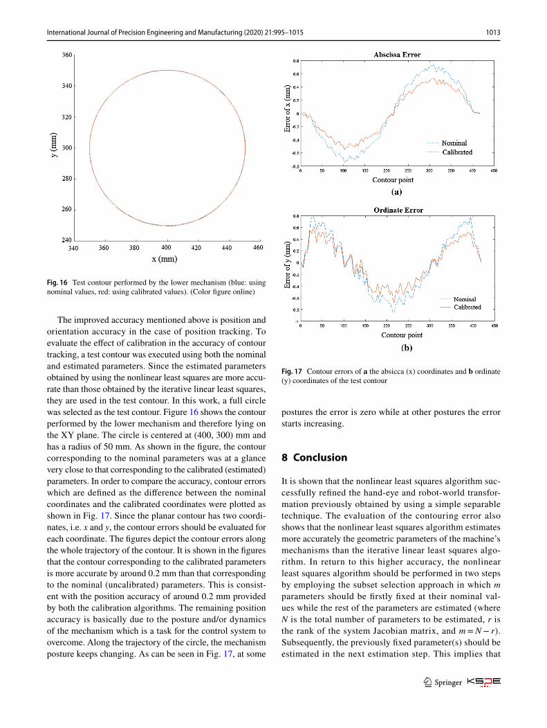
The improved accuracy mentioned above is position and orientation accuracy in the case of position tracking. To evaluate the effect of calibration in the accuracy of contour tracking, a test contour was executed using both the nominal and estimated parameters. Since the estimated parameters obtained by using the nonlinear least squares are more accu-rate than those obtained by the iterative linear least squares, they are used in the test contour. In this work, a full circle was selected as the test contour. Figure 16 shows the contour performed by the lower mechanism and therefore lying on the XY plane. The circle is centered at (400, 300) mm and has a radius of 50 mm. As shown in the figure, the contour corresponding to the nominal parameters was at a glance very close to that corresponding to the calibrated (estimated) parameters. In order to compare the accuracy, contour errors which are defined as the difference between the nominal coordinates and the calibrated coordinates were plotted as shown in Fig. 17. Since the planar contour has two coordi-nates, i.e. x and y, the contour errors should be evaluated for each coordinate. The figures depict the contour errors along the whole trajectory of the contour. It is shown in the figures that the contour corresponding to the calibrated parameters is more accurate by around 0.2 mm than that corresponding to the nominal (uncalibrated) parameters. This is consist-ent with the position accuracy of around 0.2 mm provided by both the calibration algorithms. The remaining position accuracy is basically due to the posture and/or dynamics of the mechanism which is a task for the control system to overcome. Along the trajectory of the circle, the mechanism posture keeps changing. As can be seen in Fig. 17, at some

postures the error is zero while at other postures the error starts increasing.

8 Conclusion

It is shown that the nonlinear least squares algorithm suc-cessfully refined the hand-eye and robot-world transfor-mation previously obtained by using a simple separable technique. The evaluation of the contouring error also shows that the nonlinear least squares algorithm estimates more accurately the geometric parameters of the machine’s mechanisms than the iterative linear least squares algo-rithm. In return to this higher accuracy, the nonlinear least squares algorithm should be performed in two steps by employing the subset selection approach in which m parameters should be firstly fixed at their nominal val-ues while the rest of the parameters are estimated (where N is the total number of parameters to be estimated, r is the rank of the system Jacobian matrix, and m = N − r). Subsequently, the previously fixed parameter(s) should be estimated in the next estimation step. This implies that

Fig. 16 Test contour performed by the lower mechanism (blue: using nominal values, red: using calibrated values). (Color figure online)

Fig. 17 Contour errors of a the absicca (x) coordinates and b ordinate (y) coordinates of the test contour


1 3

the fixed parameter(s) in the first step should have a con-siderably accurate value. Among all the estimated param-eters, the parameter(s) which is believed to have the most accurate value(s) can be chosen as the fixed parameter(s). Such dependency to the nominal values of the parameters does not only occur in this situation; it also occurs in the hand-eye and robot-world calibration which assumes some degree of accuracy of the nominal values of the mecha-nism geometric parameters. On the other hand, the closed-form solution of the linear least squares should be iterated until it converges to the actual values. Otherwise, it may give estimates of the parameters that are worse than the nominal values due to divergence from the actual values. Finally, using the compensated kinematics, it is shown that both the position tracking error and the contour tracking error were reduced.

Acknowledgements This research was partially supported by the Khalifa University Internal Research Fund.

Open Access This article is distributed under the terms of the Crea-tive Commons Attribution 4.0 International License (http://creat iveco mmons .org/licen ses/by/4.0/), which permits unrestricted use, distribu-tion, and reproduction in any medium, provided you give appropriate credit to the original author(s) and the source, provide a link to the Creative Commons license, and indicate if changes were made.

References

1. Merlet, J.-P. (2006). Parallel robots (2nd ed.). Dordrecht: Springer.

2. Bai, S., & Theo, M. Y. (2003). Kinematic calibration and pose measurement of a medical parallel manipulator by optical position sensors. Journal of Robotic Systems, 20(4), 201–209.

3. Altuzarra, O., et al. (2009). Parallel kinematics for machine tools, in machine tool for high performance machining. London: Springer.

4. Roth, Z. S., Mooring, B., & Ravani, B. (1987). An overview of robot calibration. IEEE Journal of Robotics and Automation, 3(5), 377–385.

5. Vischer, P., & Clavel, R. (1998). Kinematic calibration of the par-allel Delta robot. Robotica, 16, 207–218.

6. Yang, Z., Cheon, S.-U., & Yang, J. (2013). A kinematic calibration method of a 3-DOF secondary mirror of the giant Magellan. Jour-nal of Mechanical Sciences and Technology, 27(12), 3779–3786.

7. Patel, A. J., & Ehmann, K. F. (2002). Calibration of a hexapod machine tool using a redundant leg. International Journal of Machine Tools and Manufacture, 40, 489–512.

8. Iurascu, C., & Park, F. C. (2003). Geometric Algorithms for Kin-ematic Calibration of Robots Containing Closed Loops. Journal of Mechanical Design, 125(1), 23–32.

9. Yu, D. (2011). Kinematic calibration of a parallel robot using coordinate measuring machine. International Journal of the Phys-ical Sciences, 6(21), 4999–5004.

10. Wang, L.-P., et al. (2011). Kinematic calibration of the 3-DOF parallel module of a 5-axis hybrid milling machine. Robotica, 29, 535–546.

11. Wang, Y., Wu, H., & Handroos, H. (2011). Markov Chain Monte Carlo (MCMC) methods for parameter estimation of a novel hybrid redundant robot. Fusion Engineering and Design, 88, 1863–1867.

12. Liu, Y., et al. (2007). Calibration of a Steward Parallel robot using genetic algorithm. In IEEE International Conference on Mechatronics and Automation. Harbin, China.

13. Fan, C., et al. (2015). Calibration of a parallel mechanism in a serial-parallel polishing machine tool based on genetic algorithm. International Journal of Advanced Manufacturing Technology, 81, 27–37.

14. Lee, K.-I., Lee, J.-C., & Yang, S.-H. (2018). Optimal on-machine measurement of position-independent geometric errors for rotary axes in five-axis machines with a universal head. International Journal of Precision Engineering and Manufacturing, 19(4), 545–551.

15. Lee, D.-M., et al. (2011). Identification and measurement of geo-metric errors for a five-axis machine tool with a tilting head using a double ball-bar. International Journal of Precision Engineering and Manufacturing, 12(2), 337–343.

16. Chen-Gang, et al. (2014). Review on kinematics calibration tech-nology of serial robots. International Journal of Precision Engi-neering and Manufacturing, 15(8), 1759–1774.

17. Rosyid, A., El-Khasawneh, B. S., & Alazzam, A. (2018). Genetic and hybrid algorithms for optimization of non-singular 3PRR planar parallel kinematics mechanism for machining application. Robotica, 36, 1–26.

18. Chen, D., et al. (2018). A Compensation method for enhancing aviation drilling robot accuracy based on Co-Kriging. Interna-tional Journal of Precision Engineering and Manufacturing, 19(8), 1133–1142.

19. Tsai, R. Y., & Lenz, R. K. (1989). A new technique for fully autonomous and efficient 3D robotics hand-eye calibration. IEEE Transactions on Robotics and Automation, 5(3), 345–358.

20. Daniilidis, K. (1999). Hand-eye calibration using dual quater-nions. The International Journal of Robotics Research, 18(3), 286–298.

21. Strobl, K.H. & Hirzinger, G. (2006). Optimal hand-eye calibra-tion. In International Conference on Intelligent Robots and Sys-tems 2006. Beijing, China.

22. Shah, M. (2013). Solving the robot-world/hand-eye calibration problem using the Kronecker product. Journal of Mechanisms and Robotics, 5(3), 031007.

23. Heller, J., Henrion, D, & Pajdla, T. (2014). Hand-eye and robot-world calibration by global polynomial optimization. In IEEE International Conference on Robotics and Automation (ICRA ) 2014. Hong Kong, China

24. Dornaika, F., & Horaud, R. (1998). Simultaneous robot-world and hand-eye calibration. IEEE Transactions on Robotics and Automa-tion, 14(4), 617–622.

25. Li, A., Wang, L., & Wu, D. (2010). Simultaneous robot-world and hand-eye calibration using dual-quaternions and Kronecker product. International Journal of the Physical Sciences, 5(10), 1530–1536.

26. Ernst, F., et al. (2012). Non-orthogonal tool/flange and robot/world calibration. International Journal of Medical Robotics, 8(4), 407–420.

http://creativecommons.org/licenses/by/4.0/

http://creativecommons.org/licenses/by/4.0/


1 3

27. Li, H., et al. (2016). Simultaneous hand-eye and robot-world cali-bration by solving the AX = YB problem without correspondence. IEEE Robotics and Automation Letters, 1(1), 145–152.

28. Liu, Y., et al. (2017). Simultaneous calibration of hand-eye rela-tionship. Robot-World Relationship and Robot Geometric Param-eters with Stereo Vision, 710, 462–475.

29. Zhi X, Schwertfeger S (2017) Simultaneous hand-eye calibra-tion and reconstruction. In IEEE/RSJ International Conference on Intelligent Robots and Systems (IROS) 2017. Vancouver, BC, Canada.

30. Zhao, Z. (2018). Simultaneous robot-world and hand-eye calibra-tion by the alternative linear programming. Pattern Recognition Letters.

31. Zhuang, H., Roth, Z. S., & Sudhakar, R. (1994). Simultaneous robot-world and tool-flange calibration by solving homogeneous transformation equations of the form AX = YB. IEEE Transac-tions on Robotics and Automation, 10(4), 549–554.

32. Gauss, K. F. (1963). Theory of the motion of the heavenly bodies moving about the sun in conic sections. A translation of Theoria Motus. New York, NY: Dover Publications.

33. Saaty, T. L. (1981). Modern nonlinear equations. NY: Dover Publications.

34. Crassidis, J. L., & Junkins, J. L. (2012). Optimal estimation of dynamic systems (2nd ed.). Boca Raton: CRC Press.

Publisher’s Note Springer Nature remains neutral with regard to jurisdictional claims in published maps and institutional affiliations.

Abdur Rosyid received his Ph.D. in Engineering from Khalifa University of Science and Tech-nology, Abu Dhabi, UAE. He is currently working as a post-doc-toral research fellow at the same university. His research interests include parallel and hybrid kin-ematics mechanisms (kinemat-ics, dynamics, gravity compen-s a t i o n , c o n t r o l , d e s i g n optimization, and parameter estimation) as well as robotics for manufacturing.

Bashar El‑Khasawneh is currently the chair of the graduate pro-gram at the Mechanical Engi-neering Department and an asso-ciate professor of mechanical engineering at Khalifa Univer-sity. He served as the Associate Chair for the department from 2013-2016. Before that he acted as an academic advisor for the British University in Dubai to develop an accredited industrial engineering program. Between 2008 and 2010 he was the Man-ager of the Applied Research Programs at King Abdullah II

Design and Development Bureau (KADDB), Jordan. Between 2002 to 2008 he held an assistant professor position in the Industrial Engineer-ing Department, at Jordan University of Science and Technology

(JUST), within that time he served as a chairman for the department for two years. Between 1998-2002 he worked for Caterpillar Incorpo-rated in the technical center and for KLA-Tencor with the technology group both in USA. He worked extensively on technical and managerial assistance for many industries. He founded a design and development pre-incubator at the JUST University to train and qualify students to become entrepreneurs. He obtained his PhD in Mechanical Engineering from University of Illinois at Urbana-Champaign, USA (1997). He is a member of the Advisory Board of the Innovation Lab at the Dubai Health Authority (DHA) and a member of the editorial board of IJAER. His current research is focused on developing new concepts of advanced machining centers based on parallel kinematics mechanism and machining in harsh environments by adapting to the environment/geometry and be able to perform machining/welding tasks.

Anas Alazzam is an Associate Professor in the Mechanical Engineering Department at Khalifa University, Abu Dhabi, UAE. Prior to joining Khalifa University in 2012, he was part of the research and development team at the Canadian Space Agency (CSA), Saint Hubert, Canada. He completed his PhD in the area of Micro-Electro Mechanical Systems (MEMS) in 2010 from Concordia University, Montreal, Canada. He has research background in microflu-idics, Dielectrophoresis, and

healthcare applications of microdevices. He contributed to advance-ment of knowledge in the field of separation using micro-fluidic means. Dr. Alazzam has published over 80 peer reviewed papers in prestigious journals and conferences and a member of several academic associa-tions. His research interests include microsystems, cells separation, micro- and macro- fabrication, and bio-applications of microfluidic systems.

external kinematic calibration of hybrid kinematics ... · external kinematic calibration of hybrid...

Documents