Descriptive Geometric Kinematic Analysis

of Clavel’s “Delta” Robot

P.J. Zsombor-MurrayMcGill University

Department of Mechanical EngineeringCentre for Intelligent Machines

Rm. 454, 817 Sherbrooke St. W.Montreal (Quebec) Canada, H3A 2K6

<paul@cim.mcgill.ca>

April 1, 2004

Abstract Certain high speed industrial assembly robots share a peculiarthree legged parallel architecture wherein three “hips”, attached to a fixedupper base or “pelvis”, actuate “thighs” connected by “knees” to “shins”.Each shin is a parallelogramic four-bar linkage. “Ankles” are connected toa common end effector “foot” which executes spatial translatory motion.Inverse and direct kinematic analyses of such manipulators have simple ge-ometric solutions reducable to intersection of line and sphere. Computationis carried out efficiently in a common fixed reference frame.

1 Introduction

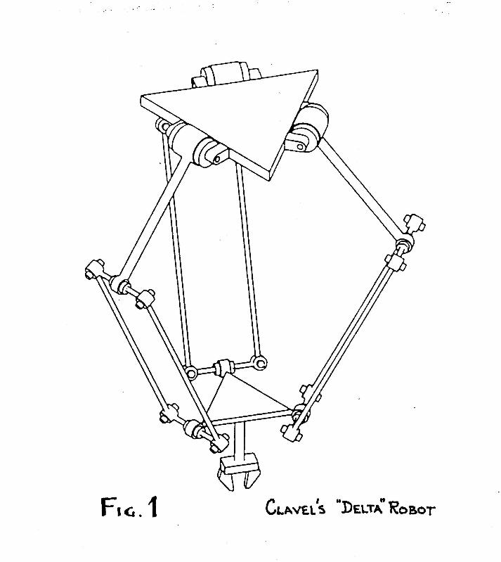
In 1988 Clavel introduced a three degree of freedom(dof), three identicallegged manipulator he called “Delta”. This device is shown in Fig. 1. Itsend effector(EE) or “foot” executes pure spatial translation.

1.1 Description

The fixed frame(FF) or “pelvis” supports three actuated revolute(R) jointed“hips”. These R-axes form an equilateral planar triangle. The “knee” endof each “thigh” supports another R-joint whose axis is parallel to the oneat the hip. The foot also supports three R-joints whose axes form anothertriangle which is similar to and maintains the same orientation as the one

1

on FF. The EE triangle R-axes are held parallel to those on FF because the“shin” is a parallelogram four bar linkage whose R-axes are all perpendicularto the hip, knee and “ankle” R-axes. One pair of linkage R-axes intersectsthe knee R-axis while the other pair intersects the ankle R-axis.

1.2 Kinematic Geometry

It is important to note that when a thigh angle is determined by the actuator,the R-axis of the ankle, if disconnected from EE, would be free to movein the parallel line bundle of the hip R-axis. Note also the three pointsDi, Ei, Ci, i = 1, 2, 3, at hip, knee and ankle of each leg as shown inFig. IKDELTA. Di is the midpoint of a FF R-joint axis triangle side. Ei

is the point on a knee R-joint axis midway between the parallel axis R-joint pair of the four bar linkage while Ci is midway on the opposite link,coincident with an EE R-joint axis triangle side. If disconnected from thefoot, Ci would move on the sphere centred on Ei. Similarly, if EE were fixedand Ei were freed at the knee then Ei would describe a sphere of the sameradius centred on Ci.

1.3 Rationale

Why embark on a reprise of old developments? “Delta” is mentioned in arecent book by Angeles[1]. The elegant symmetry of this robot and its fine,relatively singularity free simplicity, albeit embedded in apparent complex-ity, were found to be quite compelling. Clavel’s original work, mentioned atthe outset, was not cited because it was not readily available for examinationhowever the inverse kinematics of “Delta” was treated by Pierrot[2]. It wasimplied that a leg chain closure equation approach described therein rep-resented substantial improvement in this regard. His outline of the directproblem relied on three of these quadratic equations. Obviously, numeri-cal solution is required here. Also relevant is work by Herve[3] wherein ageometrically very similar translational robot, using prismatic rather thanrevolute actuation, was dealt with. This one, called “Y-Star”, (Notice thetransference of the star-delta transformation from its commonly encounteredconnection with three-phase electrical power.) has screw actuated P-jointedhips. Precise kinematic analysis must be a nightmare because when theplane of a four bar thigh swings on its screw axis, it introduces a parasiticP-joint displacement shift! Only an inverse kinematic analysis was done,this time using the notion of intersecting Schonflies displacement subgoups.In fact, considering the difficult-to-follow analysis and certain obvious alge-

2

braic errors, it seems the purpose of that article was to expose the liason ofgroups and not so much to facilitate motion computations. That is the pur-pose of this article: to provide a clear kinematic analysis useful to those whomay wish to program and employ nice little three legged robots suited to aline and sphere intersection model. If one is interested in pursuing historicaldetail and past research on “Delta” and its cousins, many relavent referencesappear in the three documents listed in the bibliography and cited above.

2 Analysis

Now let us examine the inverse and direct kinematics via geometric con-structions. These are easy to understand. Computation is based on similar,but not quite identical, geometry.

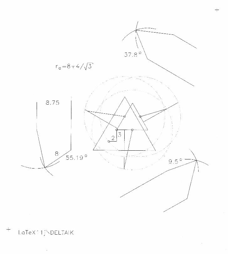
2.1 Inverse Kinematic Construction

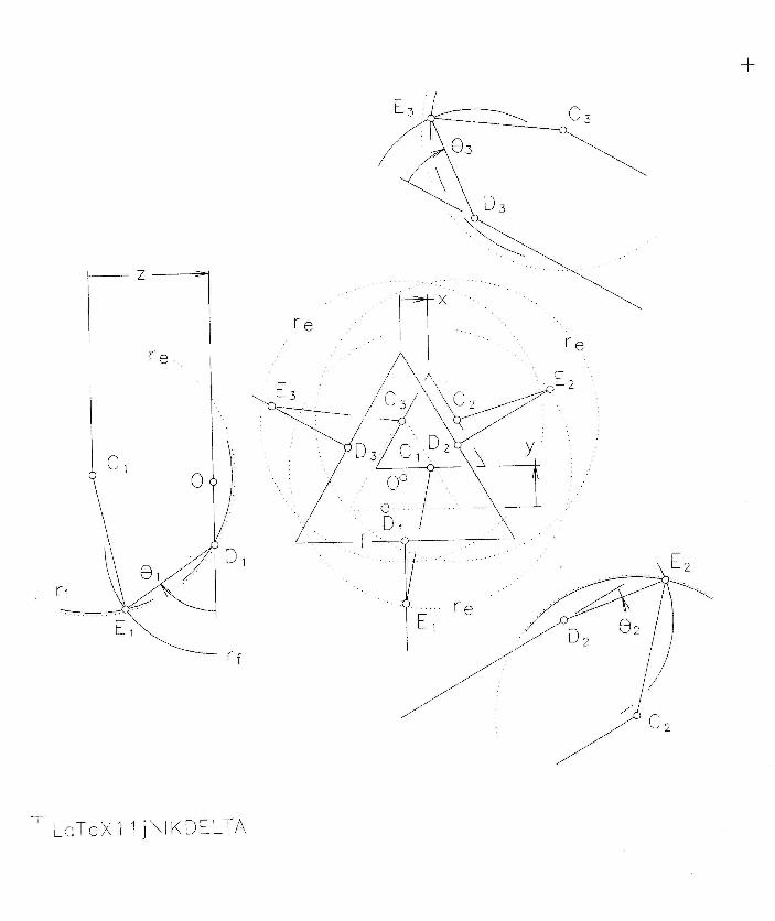
Fig. IKDELTA shows a top view of the two triangular platforms. The ninekey points, Di, Ei, Ci, are clearly visible. The centre of the smaller EE isdisplaced by (x, y, z) from origin O at the centre of FF. Note the designconstants. e is the side length of EE, f the side of FF, re the distance CiEi

and rf the distance DiEi. A sphere, radius re, centred on Ci gives the locusof Ei. Furthermore a second constraint is imposed by the circular trajectoryof Ei at radius rf from centre Di. The plane of this circle is visible as a line.The plane cuts the sphere in a small circle in the same plane. In the threeauxiliary elevation views one sees this small circle inside the dotted outline ofthe sphere. The other solid arc is the circle centred on Di. The intersectionof the arcs yield Ei, the solution external to FF and EE is chosen as theobviously valid one. The desired actuated R-joint angles are measured fromthe edge or line view of FF to DiEi as θi. The leg subscript i is omittedin all the following equations. It is obvious that a joint angle θ must becomputed separately for each leg.

2.2 Inverse Kinematic Computation

In this case a line will be intersected not with the sphere described above,centred on ankle C, but with the algebraically simpler one on D. Thehomogeneous coordinates E{w : x : y : z} of a point on it are given by

(xdw − x)2 + (ydw − y)2 + (zdw − z)2 − rfw2 = 0 (1)

3

where zd = 0 in the frame chosen. Which line? The one through thetwo desired solutions for E. It is obtained by intersecting the plane ofa thigh circle centred on D with the plane of a circle produced by theintersection of the sphere given by Eq. 1 and one of radius re centred onC. The homogeneous coordinates of the three vertical thigh planes, π{Wπ :Xπ : Yπ : Zπ} on O can be written by inspection.

π1{0 : 1 : 0 : 0}, π2{0 : 1 : −√

3 : 0}, π3{0 : 1 :√

3 : 0}

For those not familiar with homogeneous plane coordinates, the last threeare normal direction numbers, the first is the moment of the normal directionvector. Since all three planes are on O, the first coordinates Wπ are all zero.Coordinates of the plane of the circle of intersection between the spherescentred on C and D are the coefficients of the linear equation which isthe difference between the two sphere equations. Its plane coordinates are{Wi : Xi : Yi : Zi}. Explicitly, a thigh and shin sphere intersection circleplane has coordinates

{(r2e − r2

f + x2d − x2

c + y2d − y2

c − z2c )/2 : (xc − xd) : (yc − yd) : zc}

The next step is to compute radial Plucker coordinates of the line, i.e.,switching the first and second triplets of the axial coordinates obtained withplane intersection. Expanding on all 2× 2 minor subdeterminants∣∣∣∣∣ Wπ Xπ Yπ Zπ

W X Y Z

∣∣∣∣∣ ⇒ {p01 : p02 : p03 : p23 : p31 : p12}

Finally, for the second constraint, recall the point-on-line relationship.0 p23 p31 p12

−p23 0 p03 −p02

−p31 −p03 0 p01

−p12 p02 −p01 0

wxyz

=

0000

(2)

The second and third lines of Eq. 2, a doubly rank deficient system of fourlinear equations, are substituted into Eq. 1 to produce Eq. 3, a quadratic inz = ze. This is all that is needed to find θ = sin−1(ze/rf ).

4

[(p01

p03

)2

+(

p02

p03

)2]

z2

−2[p01

p03

(p31

p03+ xd

)− p02

p03

(p23

p03− yd

)]wz

+

[(p31

p03+ xd

)2

+(

p23

p03− yd

)2

+ z2d − r2

f

]w2 = 0 (3)

Simplifications arise due to choice of frame. Note p12 = 0 and for z1, p01 =p31 = 0 as well. This may be coded at computational expense similar tothat incurred in Pierrot’s[2] solution however the additional trigonometryof his rotation matrix is not necessary. A programmed example could nowbe easily presented but that will be saved for the following direct kinematicanalysis where the algebraic geometric detail above will not be repeated butthe efficacy of a simple algorithm will be shown instead.

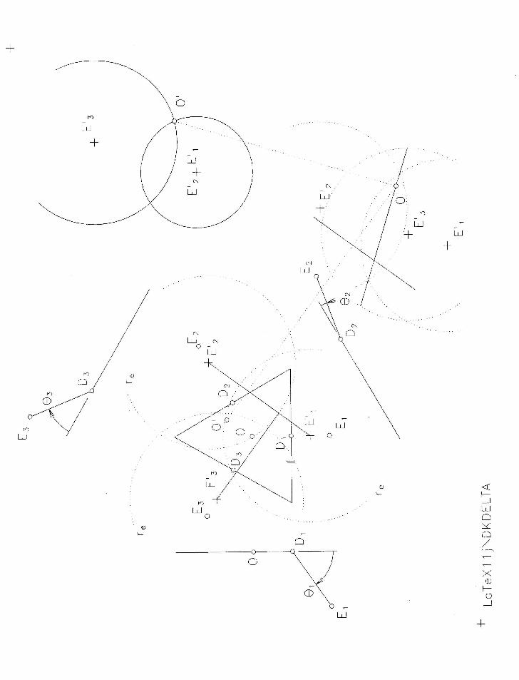
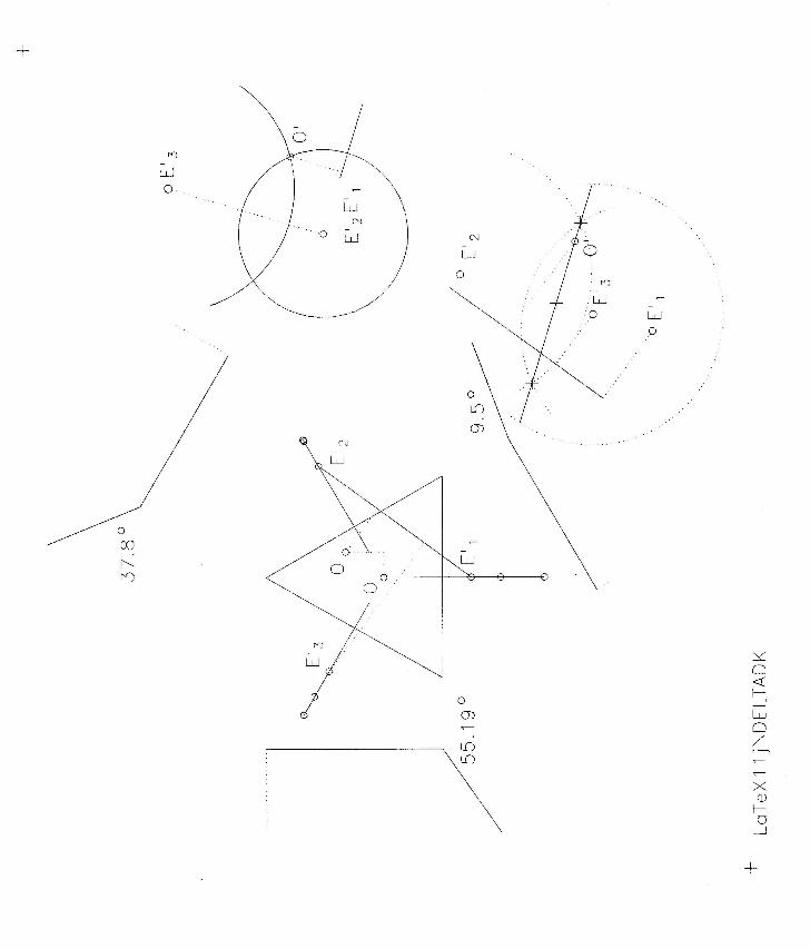
2.3 Direct Kinematic Construction

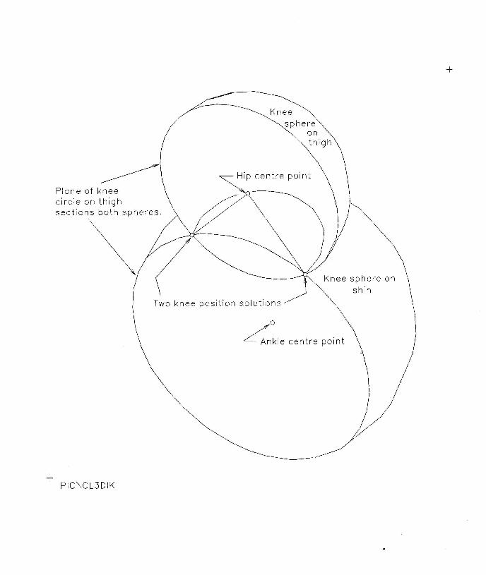
Now consider Fig. DKDELTA. EE pose and manipulator design constantsare identical to those selected for the inverse kinematic example shown inFig. IKDELTA. This time the three angles θi are given instead of the po-sition of the EE centre point, shown as O′, which must be determined.The geometric key to the direct kinematic solution is the location of pointsE′

i which serve as centres of three spheres, radius re. Their two intersec-tion points define two possible solution poses. The constructive solution isshown in a second auxiliary view where the circle of intersection on spherescentered on E′

1 and E′2 defines a plane which sections the sphere on E′

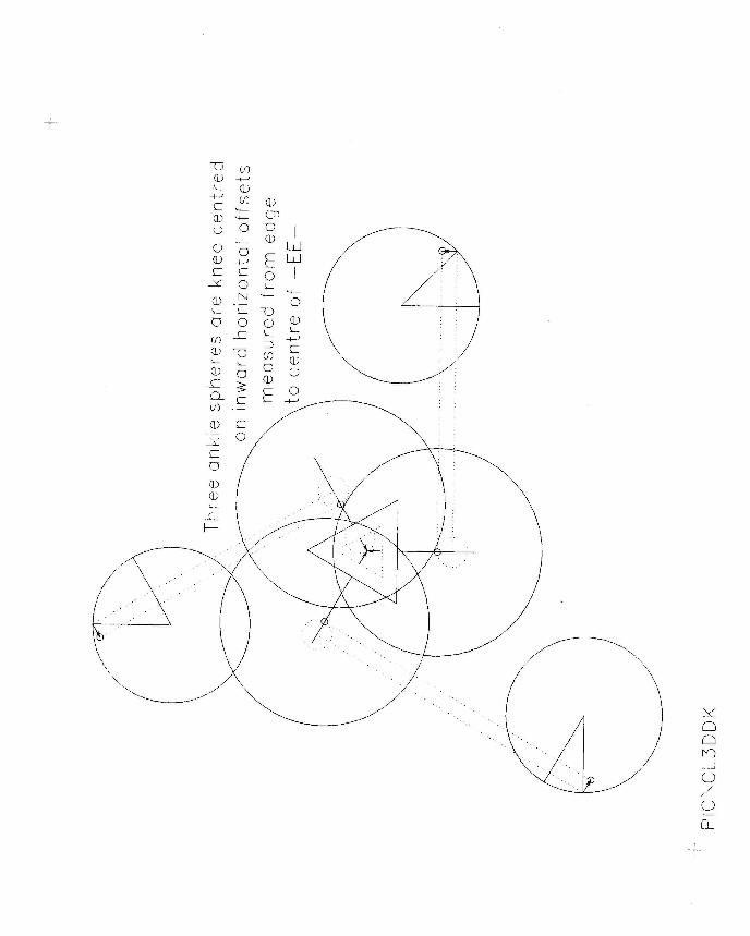
3 ona second coplanar circle. The intersections of the two circles are obtainedhere by inspection and projected to the first auxiliary view which showsthe FF plane in edge or line view. The lower point is chosen as O′ andthe z-coordinate can be measured here. Projection of this point into thetop view provides the other two coordinates. But how are the points E′ilocated? Angles θi fix Ei but the free ankles on the shins centred on thefixed knees Ei describe spheres that contain Ci, respectively, not O′. Noticethat O′ is located from Ci by three displacement vectors of constant lengthand constant direction, pointing inward on EE. Therefore to maintain puretranslation of EE, O′ must move on three spheres whose centres are similarlydisplaced, horizontally inward.

5

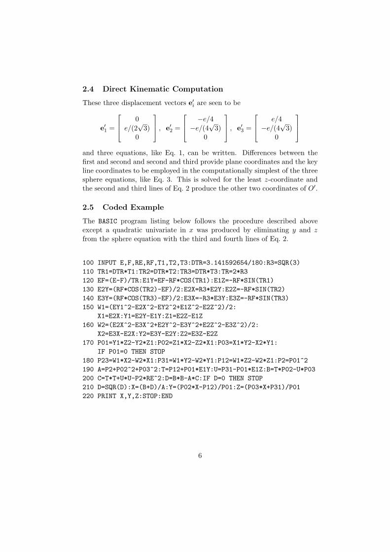
2.4 Direct Kinematic Computation

These three displacement vectors e′i are seen to be

e′1 =

0e/(2

√3)

0

, e′2 =

−e/4−e/(4

√3)

0

, e′3 =

e/4−e/(4

√3)

0

and three equations, like Eq. 1, can be written. Differences between thefirst and second and second and third provide plane coordinates and the keyline coordinates to be employed in the computationally simplest of the threesphere equations, like Eq. 3. This is solved for the least z-coordinate andthe second and third lines of Eq. 2 produce the other two coordinates of O′.

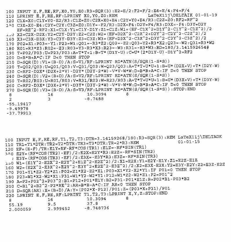
2.5 Coded Example

The BASIC program listing below follows the procedure described aboveexcept a quadratic univariate in x was produced by eliminating y and zfrom the sphere equation with the third and fourth lines of Eq. 2.

100 INPUT E,F,RE,RF,T1,T2,T3:DTR=3.141592654/180:R3=SQR(3)110 TR1=DTR*T1:TR2=DTR*T2:TR3=DTR*T3:TR=2*R3120 EF=(E-F)/TR:E1Y=EF-RF*COS(TR1):E1Z=-RF*SIN(TR1)130 E2Y=(RF*COS(TR2)-EF)/2:E2X=R3*E2Y:E2Z=-RF*SIN(TR2)140 E3Y=(RF*COS(TR3)-EF)/2:E3X=-R3*E3Y:E3Z=-RF*SIN(TR3)150 W1=(EY1^2-E2X^2-EY2^2+E1Z^2-E2Z^2)/2:

X1=E2X:Y1=E2Y-E1Y:Z1=E2Z-E1Z160 W2=(E2X^2-E3X^2+E2Y^2-E3Y^2+E2Z^2-E3Z^2)/2:

X2=E3X-E2X:Y2=E3Y-E2Y:Z2=E3Z-E2Z170 P01=Y1*Z2-Y2*Z1:P02=Z1*X2-Z2*X1:P03=X1*Y2-X2*Y1:

IF P01=0 THEN STOP180 P23=W1*X2-W2*X1:P31=W1*Y2-W2*Y1:P12=W1*Z2-W2*Z1:P2=P01^2190 A=P2+P02^2+P03^2:T=P12+P01*E1Y:U=P31-P01*E1Z:B=T*P02-U*P03200 C=T*T+U*U-P2*RE^2:D=B*B-A*C:IF D=0 THEN STOP210 D=SQR(D):X=(B+D)/A:Y=(P02*X-P12)/P01:Z=(P03*X+P31)/P01220 PRINT X,Y,Z:STOP:END

6

3 Conclusion

It was mentioned at the beginning that this type of manipulator is relativelyfree of singularity. The the ones that may occur are readily anticipated, likeif a leg is fully extended or folded, one experiences three coplanar parallelR-axes. Similarly obvious are the four bar linkage dead-centre singularities.All seem restricted to conditions confined to a leg. However, due to symme-try the conditions may arise simultaneously in all three legs. Carrying out asingularity surface mapping in the kinematic image space may be an inter-esting exercise but is hardly necessary to achieve fairly trouble free operationof “Delta” type robots. A more interesting issue is the indication that threedof, three legged spatial robots have inverse and direct kinematic solutionsof similar complexity. Even six dof robots with three legs, each with twoactuators, have, in general, have eight or fewer assembly modes. More tothe point, one sees the line and sphere solution paradigm in Stewart-Goughplatforms with six P-joint actuated legs where three legs converge to a singleS-joint support and two others meet on a rigid body supporting a secondS-joint thus creating an effective three legged manipulator. Notwithstandingall this conjecture, it is claimed that the simplest quadratic direct solutionfor “Delta” manipulators has been exposed for the first time herein.

Acknowledgement This work is supported by FCAR (Quebec) and NSERC(Canada) research grants.

References

[1] Angeles, J. (1997): Fundamentals of Robotic Mechanical Systems: The-ory, Methods & Algorithms, Springer, ISBN 0-387-94540-7, pp.8-11.

[2] Pierrot, F., Fournier, A. & Dauchez, P. (1991): “Towards a Fully-ParallelSix DOF Robot for High-Speed Applications”, Proc. IEEE Rob. & Au-tom. Conf., Sacramento, ISBN 0-8186-2163-X, pp.1288-1293.

[3] Herve, J.-M. & Sparacino, F. (1992): “Star, a New Concept in Robotics”,Proc. 3ARK Wkshp., Ferrara, (Parenti-Castelli, V. & Lenarcic, J, .eds.),ISBN 88-86141-00-9, pp.176-183.

7