july 2010 njdep ebs final report: volume ii 7.0 … 7.pdf · july 2010 njdep ebs final report:...

JULY 2010 NJDEP EBS FINAL REPORT: VOLUME II

7-1

7.0 NEXRAD There is widespread interest in the environmental impacts of wind development on wildlife in general and migratory birds and bats in particular (GAO Report 2005). To assess the risk of a proposed wind project on wildlife, preconstruction studies are needed. The results of the studies provide an information base for the preparation of formal risk assessments that are considered before final approval is given for project construction. In the case of migratory birds, the avian risk assessment requires information on the changing densities of migrants in the atmosphere from hour-to-hour, day-to-day, and year-to-year (temporal patterns) and the altitudinal and geographical distribution of the migrants relative to the project and surrounding areas (spatial patterns). Although marine radar can be used in pre-construction studies of bird movements through a project area (e.g., Mabee et al. 2006), the spatial coverage is limited to a range of 1-6 NM from the radar depending on the power of the marine radar. In order to gather migration data at greater ranges (out to 100 NM or 185.2 km), larger surveillance radars must be used. In the U.S., one can use Doppler weather surveillance radar (WSR-88D) to detect, quantify, and monitor biological targets in the atmosphere (e.g., bird migration [Gauthreaux and Belser 1998, 1999; Gauthreaux et al. 2000; Gauthreaux and Belser 2003; Diehl and Larkin 2005], bird roosts [Russel and Gauthreaux 1998; Russell et al. 1998], bat colonies [McCracken 1996; McCracken and Westbrook 2002; Horn and Kunz 2008], and concentrations of insects aloft [Westbrook and Wolf 1998]). Although the lowest tilt of the 1°-beam of the WSR-88D is 0.5° above the horizontal, and the base of the beam is too high to detect low flying targets over most of the radar's surveillance sweep, the radar can be used to obtain information on the temporal and geographical aspects of bird migration because most bird migration occurs at altitudes higher than 250 m (820 ft) above ground level (Nisbet 1963; Able 1970; Bellrose 1971). If one documents the variability in the quantity of migration over a project area for several years and couples this information with the occurrence of weather conditions that cause migrants to fly at low altitudes, one can estimate the number of occasions per season when collision events could theoretically occur. This is valuable information for the comprehensive avian risk assessment. The following report presents the results of a baseline study that examines nocturnal bird migration patterns over coastal and offshore New Jersey and is intended to assist the NJDEP in the assessment of the risks that offshore wind development poses to migratory birds. 7.1 EQUIPMENT AND METHODS 7.1.1 WSR-88D The WSR-88D, also referred to as NEXRAD during the planning and development stages, is the backbone of the national network of weather radars in the U.S. operated by National Weather Service (NWS) in the National Oceanic and Atmospheric Administration (NOAA) of the Department of Commerce, the Department of Defense (units at military bases), and non-CONUS Department of Transportation Areas. There are 155 WSR-88D radars in the nation, including the U.S. Territory of Guam and the Commonwealth of Puerto Rico. Components and operational details of the radar system can be found in Crum and Alberty (1993), Crum et al. (1993) and Klazura and Imy (1993). Additional characteristics of the WSR-88D can be found in Appendix L-1. 7.1.2 Methods For this study archived WSR-88D data from the KDIX station (Figure 7-1) were analyzed to characterize the migration patterns of birds over the coastal region of New Jersey during the spring (15 March to 31 May 2005-2009, 390 nights) and fall (15 August to 15 November 2005-2009, 465 nights) migration periods. This station provides exceptional coverage of the sample areas in this study (Figure 7-2). For our analysis we used the WSR-88D radar data archive at the National Climatic Data Center (NCDC) in Asheville, North Carolina. The WSR-88D radar data archive at NCDC has Level-II data from 26 April 1995


7-2

to present. We analyzed Level-II data from the NCDC archive at 0.5° antenna elevation angle for this study. We used the following protocol during our analysis: We first established six sample areas along the coastal and offshore region of New Jersey (Figure 7-3). The three coastal areas were chosen to cover the three coastal MARS® surveillance areas located at IBSP, BB, and SIC, New Jersey (areas 1A, 2A, and 3A, respectively, lettered N to S respectively). The three offshore sample areas (1B, 2B, and 3B, lettered N to S respectively) were created approximately 13 to 15 km offshore and parallel with the onshore sample areas. WSR-88D Level II data are in radial raster (1 km x 1° for base reflectivity data and 0.25 km x 1° for radial velocity data). Thus the reflectivity data array consists of 360 radials with each radial having 240 one-kilometer bins. In the fall of 2008 the NWS upgraded the existing NEXRAD stations and increased the resolution of the base reflectivity and radial velocity to 0.25 km x 0.5° resulting in an array consisting of 720 radials with each having 960 0.25-km bins. Matching (same volume scan) base reflectivity and base velocity data were downloaded from the NCDC archives for the evening hours of every 24-hr period during spring and fall migration (15 April through 31 May and 15 August through 15 November). Base reflectivity data files provide information on the density of targets in the atmosphere, and base velocity data files contain information on radial velocity of targets and direction of movement. We first examined the base reflectivity and velocity files for each night and eliminated those with precipitation in the sample area or with other issues such as excessive strobes and anomalous propagation of the radar beam. All information was recorded in a spreadsheet (Excel, Microsoft 2007) with a row for each evening.

Figure 7-1. Surveillance area of WSR-88D radar at KDIX. The inner range mark is 50 NM and the outer range mark is 100 NM.


7-3

Figure 7-2. Coverage pattern of the WSR-88D at Fort Dix, New Jersey. The radar antenna is 70 m (230 ft) above sea level (ASL) and the coverage pattern is above radar antenna level (arl).


7-4

Figure 7-3. Sample areas along coastal and offshore New Jersey. The Fort Dix, New Jersey WSR-88D station (KDIX) is illustrated with a “+” sign. Onshore sample areas are 1A, 2A, and 3A (N to S respectively) and offshore sample areas are 1B, 2B, and 3B (N to S respectively). We examined the series of saved base reflectivity and base velocity files without precipitation in the sample area for each evening and selected the files that showed peak density and eliminated those with excessive insect contamination and other aerial reflectors (e.g., smoke and dust particles). The latter was accomplished by comparing winds aloft with the mean speeds of targets in the base velocity images (Gauthreaux et al. 2008). Because no winds aloft data are taken at Fort Dix, New Jersey, archived winds aloft data measured at Upton, New York (KOKX) were obtained from the Department of Atmospheric Science at the University of Wyoming site. This dataset contains Radiosonde observations (RAOB) of upper-air conditions (e.g., winds aloft) for all stations in the U.S. and is available from 1973 to present. The observations are made near the beginning (00:00 UTC) and the end of the night (12:00 UTC). We saved text files and converted them into Excel spreadsheet files containing date, time (UTC), altitude (m), wind speed (m/s), and wind direction (from). If the maximum mean radial velocity of the targets was within 5 m/s (18 kph) of the velocity of following winds aloft, the associated base reflectivity file was eliminated from additional analysis because of the likelihood of insect contamination. Likewise, if winds aloft were calm and the base velocity file showed no mean radial velocities in keeping with velocities of songbirds (32.4 to 54 kph; 17.5 to 29.2 kts; Bruderer and Boldt 2001), the associated base reflectivity file was eliminated. If the maximum mean radial velocity of the targets was in keeping with birds and the direction of flight was not in the direction of the winds aloft, the base reflectivity file was saved for further analysis. Remaining mean base velocity information of at least 5 m/s above wind speed was used to determine the direction of flight and to determine the relative reflectivity values (decibels of reflectivity [dBZ]) in associated relative reflectivity pixels (1° x 1 km [pre-fall 2008]) and 0.5° x 0.25 km [fall 2008 and spring 2009] pulse volumes or resolution cells). By taking this conservative approach we were able to measure the difference between the maximum relative reflectivity in a reflectivity file and the maximum relative reflectivity of the pixels that had velocities in keeping with bird flight speeds. The former is generally greater than the latter, but in some cases the two measures are the same. The greater the difference in these two measures the more likely insects and other particulates

N


7-5

in the atmosphere are responsible for most of the relative reflectivity. Base reflectivity files with little or no reflectivity from insects or other particulates in the atmosphere were processed with an algorithm designed to measure the base reflectivity of each surviving pixel in the sample area. The base reflectivity value was converted to a Z-value and then used to compute birds per cubic kilometer (km-3; Z-value multiplied by 1.84). The sample areas in this study (11 km x 11°) have 121 radial array pixels of 1° x 1 km (pre-fall 2008) and for fall 2008 and spring 2009 have 968 radial array pixels of 0.5° x 0.25 km. The azimuth and distance (range) of the coordinates of the sample areas are given in Table 7-1, and the altitude of the radar beam over the sample areas is given in Table 7-2. The conical beam of the WSR-88D is 1° in diameter and the center of the beam is tilted 0.5° and above the horizontal. Finally, based on the results of the processing of saved reflectivity files showing peak of movement each night, we selected a subsample of nights with good movements to measure the hour-to-hour temporal pattern of nocturnal migration. Some nights with good peak reflectivity data could not be used for the hour-to-hour analysis because precipitation moved into the sample area as the night progressed. Table 7-1. Sample area distance and azimuth from Fort Dix, New Jersey WSR-88D station (KDIX).

Area Distance 1 Distance 2 Angle 1 Angle 2 Onshore

1A 27 37 117 127 2A 54 64 170 180 3A 83 93 191 201

Offshore 1B 50 60 112 122 2B 72 82 157 167 3B 92 102 175 185

Table 7-2. Altitudes sampled by the beam of the WSR-88D over the sample areas at 0.5° antenna elevation, not corrected for height of radar antenna (230 ft [70 m] AMSL).

Area Distance (km) Base (m) Center (m) Top (m) Width (m)

1A 27 63 282 501 438 32 84 345 616 519 37 111 411 711 600

2A 54 222 660 1098 876 59 261 742 1221 957 64 306 825 1344 1038

3A 83 495 1170 1845 1347 88 555 1268 1983 1428 93 618 1374 2130 1509

1B 50 192 597 1002 813 55 228 675 1122 894 60 270 756 1242 375

2B 72 381 966 1551 1170 77 432 1056 1680 1251 82 486 1152 1818 1332

3B 92 606 1353 2100 1494 97 672 1458 2244 1575 102 738 1566 2394 1656


7-6

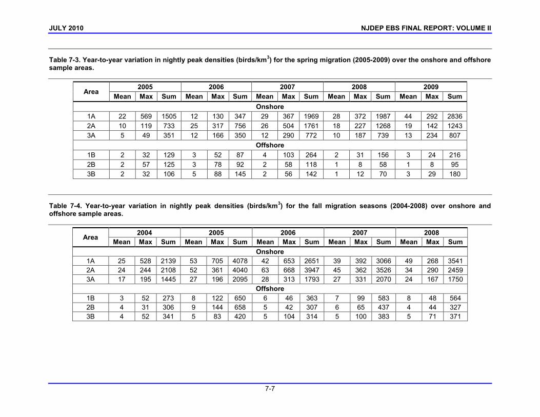
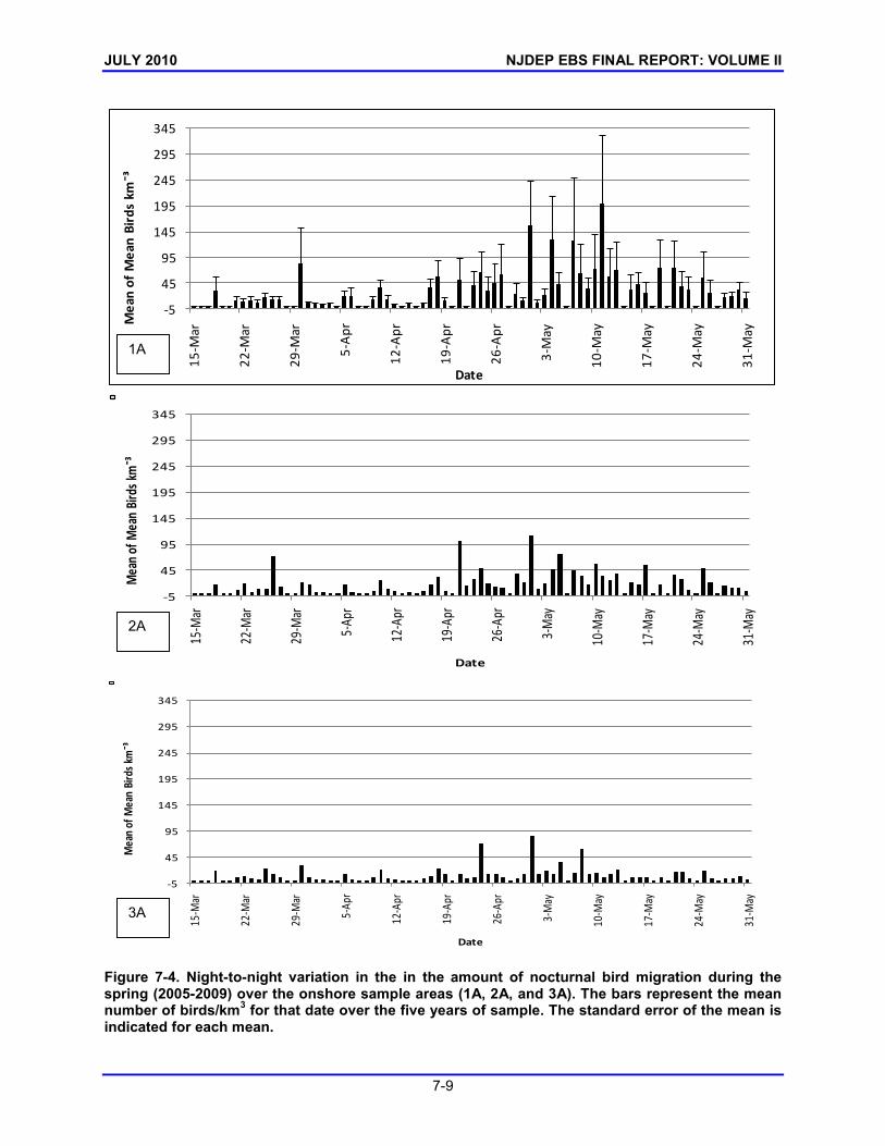
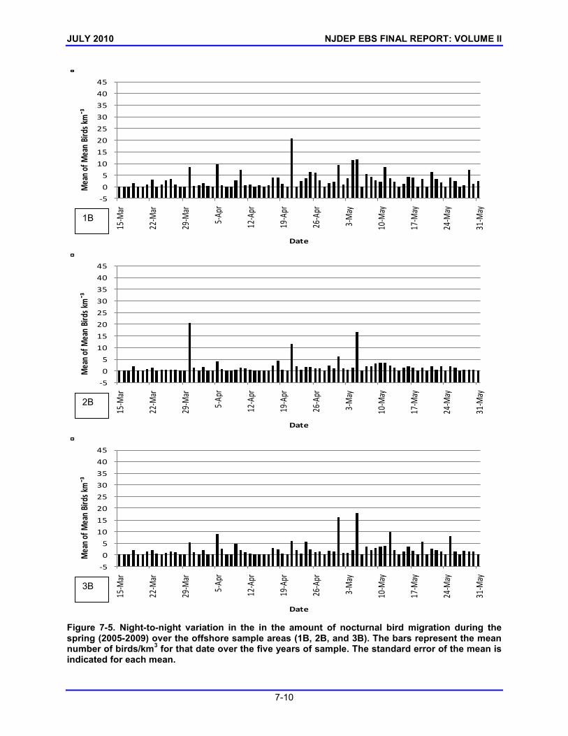
The data extracted from the base reflectivity files were analyzed with Excel to reveal the year-to-year, season-to-season, night-to-night and hour-to-hour patterns of variation in the amount of migration. The statistical analysis of the direction of migratory movements extracted from the base velocity files were analyzed with the software program Oriana 2 (Version 2.01, Kovach Computing Services, Anglesey, Wales). In an effort to determine the number of nights in a season when migrants are forced to fly low and at the same heights as man-made structures such as towers and wind turbines, we related the density of migration to weather conditions that might cause birds to fly low (Avery et al. 1977; Crawford 1981). We used data from the night-to-night peak of migration analysis and obtained local climate data (LCD) for the Atlantic City International Airport (Egg Harbor City, New Jersey) from the NCDC in Asheville, North Carolina. We recorded the nights when ceiling height was 1000 ft (305 m) or lower, the sky was overcast, and if any of the following weather conditions were present: fog, mist, rain, haze, and smoke. 7.2 RESULTS AND DISCUSSION 7.2.1 Year-to-Year Pattern of Migration The year-to-year pattern of nightly density of migratory movements derived from Level II base reflectivity files from the WSR-88D at KDIX for spring and fall can be found in Appendix L-2. During the spring the sum of nightly peak density (birds/km3) differed from year-to-year (Table 7-3). As expected, the maximum density of migration measured over the coastal sample areas differed from the maximum density over the offshore sample areas. This can be attributed to the bird’s tendency to follow the coast line during their migration. Though each of the six sample areas represent a different altitudinal zone (see Table 7-2) there is some overlap of altitudes sampled between sample areas and some of the onshore sample areas are sampling higher altitudes than the offshore sample areas (compare 2A vs. 1B and 3A vs. 2B in Table 7-2). If the migratory birds were distributed evenly throughout a specific altitudinal zone then there should be minimal differences between density measurements between sites within this zone. The data do not support this; when comparing onshore and offshore sample areas with overlapping altitudinal zones, the onshore sample area densities are much greater than the offshore sample area densities. Over the five years of spring data the sum of the nightly peak densities measured over the coastal sample areas ranged from 347 in the spring of 2006 (area 1A) to 2,836 in the spring of 2009 (area 1A), and the maximum density recorded was 569 in the spring of 2005 (area 1A). The sum of nightly peak densities recorded over the offshore sample areas ranged from 58 (area 2B) in the spring of 2008 to 264 in the spring of 2007 (area 1B), with a maximum density of 103 recorded in the spring of 2007 in area 1B. Thus during the five-year study the amount of migration in spring passing over the onshore sample areas was much higher than the amount of migration measured over the offshore sample areas. During the fall the sum of nightly peak density also differed from year-to-year (Table 7-4). Over the five years of fall data the sum of the nightly peak densities measured over the onshore sample areas ranged from 1,445 (area 3A) in the fall of 2004 to 4,078 (area 1A) in the fall of 2005, with a maximum density of 705 recorded in the fall of 2005 (area 1A). The range of the sum of nightly peak densities over the offshore sample areas ranged from 273 (area 1B) in the fall of 2004 to 658 (area 2B) in the fall of 2005, with a maximum density of 144 recorded in the fall of 2005 (area 2B). The five years of fall data showed the amount of migration passing over the onshore sample areas was much higher than the amount of migration measured over the offshore sample areas. Overall, the density of migration during the fall was on average two to three times as much as the density of migration observed during the spring. 7.2.2 Night-to-Night Pattern of Migration Data on the night-to-night pattern of nocturnal migration over the sample areas for spring (2005-2009) and fall (2004-2008) can be found in Appendix L-2. Nocturnal migration during the spring and fall shows considerable night-to-night variability. In the spring migration begins to build in late April, peaks near the middle of May, and then declines towards the end of May. This pattern can be seen in both the onshore and offshore sample areas (Figures 7-4 and 7-5, respectively). Within the three onshore areas there were five nights with a mean density of 100 birds/km3 or greater over the sample areas during the five years of spring migration (21 April, and 01, 04, 07, 11 May), while within the offshore sample areas the


7-7

Table 7-3. Year-to-year variation in nightly peak densities (birds/km3) for the spring migration (2005-2009) over the onshore and offshore sample areas.

Area 2005 2006 2007 2008 2009

Mean Max Sum Mean Max Sum Mean Max Sum Mean Max Sum Mean Max Sum Onshore

1A 22 569 1505 12 130 347 29 367 1969 28 372 1987 44 292 2836 2A 10 119 733 25 317 756 26 504 1761 18 227 1268 19 142 1243 3A 5 49 351 12 166 350 12 290 772 10 187 739 13 234 807

Offshore 1B 2 32 129 3 52 87 4 103 264 2 31 156 3 24 216 2B 2 57 125 3 78 92 2 58 118 1 8 58 1 8 95 3B 2 32 106 5 88 145 2 56 142 1 12 70 3 29 180

Table 7-4. Year-to-year variation in nightly peak densities (birds/km3) for the fall migration seasons (2004-2008) over onshore and offshore sample areas.

Area 2004 2005 2006 2007 2008 Mean Max Sum Mean Max Sum Mean Max Sum Mean Max Sum Mean Max Sum

Onshore 1A 25 528 2139 53 705 4078 42 653 2651 39 392 3066 49 268 3541 2A 24 244 2108 52 361 4040 63 668 3947 45 362 3526 34 290 2459 3A 17 195 1445 27 196 2095 28 313 1793 27 331 2070 24 167 1750

Offshore 1B 3 52 273 8 122 650 6 46 363 7 99 583 8 48 564 2B 4 31 306 9 144 658 5 42 307 6 65 437 4 44 327 3B 4 52 341 5 83 420 5 104 314 5 100 383 5 71 371


7-8

maximum was 21 on 21 April [area 1B]). Area 1A had the most nights with mean densities of 100 birds/km3 (4; 01, 04, 07, and 11 May) with Area 2A coming in second with two nights achieving this density (21 April and 01 May), while Area 3A never surpassed the 100 birds/km3 density, only achieving a peak value of 84 birds/km3 on 01 May. Within the offshore sample areas the mean migration density was considerably less than that measured over the onshore areas (mean peak density of 21 birds/km3). Though sizable flights can occur anytime from the middle of April through the middle of May, the peak of migration through the area is in early to mid-May. Nocturnal migration during the fall also varies from night-to-night. Fall migration builds in early September and peaks in mid-October to early November. After the peak in late October/early November the density of migration declines, and by mid-November very little migratory movement takes place. This pattern can be seen within both the onshore sample areas (Figure 7-6) and the offshore sample areas (Figure 7-7). There were 17 nights with a mean density of 100 birds/km3 or more within the onshore sample areas during the five years of fall migration (31 August, 01, 10, 13, 15, 23, 26, 29 September and 05, 12, 14, 15, 17, 20, 25 October, and 02, 09 November), while within the offshore sample areas there were no nights. Within the onshore sample areas both 1A and 2A achieved 10 nights with mean migration densities greater than 100 birds/km3 while Area 3A only surpassed that amount on two nights. Area 1A measured the highest density for the fall season on 15 October with a mean density of 258 birds/km3. Similar to the spring, the offshore sample area mean migration densities were considerably less than those measured within the onshore sample area. The maximum mean density only measured 34 birds/km3 on 12 September within Area 1B. The density of migration over coastal New Jersey appears to be similar to the densities observed with WSR-88D in other areas of the Northeastern U.S., while the density of migration offshore appears to much less. Black (2000) reported a peak density of approximately 110 birds/km3 from analyzed WSR-88D at Buffalo, New York (although data are limited to one night). In a study cited by Diehl et al. (2003) of the relationship between bird density data collected with a small 3-cm wavelength radar around 23:00 hrs at Brock University, St. Catherine’s, Ontario and the reflectivity measured with the WSR-88D at Buffalo, New York, Black reported mean bird densities between 20 April and 16 May 1999 that ranged from approximately 5 birds/km3 to 73 birds/km3. In a WSR-88D study of bird migration over Buffalo, New York, over five years (2002-2006) the mean density of migrants ranged from 78-154 birds/km3 in spring and 88-119 birds/km3 in fall (Gauthreaux 2007b). A Long Island, New York, WSR-88D study (Gauthreaux 2007a) showed the mean density of migrants ranged from 21-29 birds/km3 in spring (2002-2006) and 26-32 birds/km3 in fall (2001-2005). These values compare favorably with the current New Jersey study’s seasonal mean densities onshore though they are greater than those found offshore. 7.2.3 Hour-To-Hour Pattern of Migration The data showing the hour-to-hour pattern of migration over the sample areas during the spring (2005-2009) and fall (2004-2008) are in Appendix L-3. In spring, migration typically started 30-45 min after sunset, peaked on most evenings between 9:00 PM – 2:00 AM EST (02:00 – 06:00 UTC), and declined until sunrise (Figures 7-8 and 7-9). In the fall (Figures 7-10 and 7-11) the quantity of migration was greater than in the spring (see Figures 7-4 to 7-7), and the hour-to-hour pattern of percentage of peak hourly density during the evenings was shifted slightly earlier in the evening compared to that observed in spring (compare Figures 7-8 and 7-9 to 7-10 and 7-11). Like in the spring, migration typically started 30-45 min after sunset and the peak of a nightly movement generally occurred from 8:00 PM – 12:00 AM EST (01:00 – 05:00 UTC). The hour-to-hour temporal patterns of migration found in this study are similar to those found in other studies (Black 2000; Farnsworth et al 2004; Gauthreaux et al. 2005; Gauthreaux et al. 2007).


7-9

Figure 7-4. Night-to-night variation in the in the amount of nocturnal bird migration during the spring (2005-2009) over the onshore sample areas (1A, 2A, and 3A). The bars represent the mean number of birds/km3 for that date over the five years of sample. The standard error of the mean is indicated for each mean.

-5

45

95

145

195

245

295

345

15-M

ar

22-M

ar

29-M

ar

5-A

pr

12-A

pr

19-A

pr

26-A

pr

3-M

ay

10-M

ay

17-M

ay

24-M

ay

31-M

ay

Mea

n of

Mea

n Bi

rds

km¯³

Date

-5

45

95

145

195

245

295

345

15-M

ar

22-M

ar

29-M

ar

5-Ap

r

12-A

pr

19-A

pr

26-A

pr

3-M

ay

10-M

ay

17-M

ay

24-M

ay

31-M

ay

Mea

n of

Mea

n Bi

rds k

m¯³

Date

-5

45

95

145

195

245

295

345

15-M

ar

22-M

ar

29-M

ar

5-Ap

r

12-A

pr

19-A

pr

26-A

pr

3-M

ay

10-M

ay

17-M

ay

24-M

ay

31-M

ay

Mea

n of

Mea

n Bi

rds k

m¯³

Date

1A

3A

2A


7-10

Figure 7-5. Night-to-night variation in the in the amount of nocturnal bird migration during the spring (2005-2009) over the offshore sample areas (1B, 2B, and 3B). The bars represent the mean number of birds/km3 for that date over the five years of sample. The standard error of the mean is indicated for each mean.

-5

0

5

10

15

20

25

30

35

40

45

15-M

ar

22-M

ar

29-M

ar

5-Ap

r

12-A

pr

19-A

pr

26-A

pr

3-M

ay

10-M

ay

17-M

ay

24-M

ay

31-M

ay

Mea

n of

Mea

n Bi

rds k

m¯³

Date

-5

0

5

10

15

20

25

30

35

40

45

15-M

ar

22-M

ar

29-M

ar

5-Ap

r

12-A

pr

19-A

pr

26-A

pr

3-M

ay

10- M

ay

17-M

ay

24-M

ay

31-M

ay

Mea

n of

Mea

n Bi

rds k

m¯³

Date

-5

0

5

10

15

20

25

30

35

40

45

15-M

ar

22-M

ar

29-M

ar

5-Ap

r

12-A

pr

19-A

pr

26-A

pr

3-M

ay

10-M

ay

17-M

ay

24-M

ay

31-M

ay

Mea

n of

Mea

n Bi

rds k

m¯³

Date

1B

3B

2B


7-11

Figure 7-6. Night-to-night variation in the in the amount of nocturnal bird migration during the fall (2004-2008) over the onshore sample areas (1A, 2A, and 3A). The bars represent the mean number of birds/km-3 for that date over the five years of sample. The standard error of the mean is indicated for each mean.

-5

45

95

145

195

245

295

345

395

445

15-A

ug

22-A

ug

29-A

ug

5-Se

p

12-S

ep

19-S

ep

26-S

ep

3-Oc

t

10-O

ct

17-O

ct

24-O

ct

31-O

ct

7-No

v

14-N

ov

Mea

n of

Mea

n Bi

rds k

m¯³

Date

-5

45

95

145

195

245

295

345

395

445

15-A

ug

22-A

ug

29-A

ug

5-Se

p

12-S

ep

19-S

ep

26-S

ep

3-Oc

t

10-O

ct

17-O

ct

24-O

ct

31-O

ct

7-No

v

14-N

ov

Mea

n of

Mea

n Bi

rds k

m¯³

Date

-5

45

95

145

195

245

295

345

395

445

15-A

ug

22-A

ug

29-A

ug

5-Se

p

12-S

ep

19-S

ep

26-S

ep

3-Oc

t

10-O

ct

17-O

ct

24-O

ct

31- O

ct

7-No

v

14-N

ov

Mea

n of

Mea

n Bi

rds k

m¯³

Date

1A

3A

2A


7-12

Figure 7-7. Night-to-night variation in the in the amount of nocturnal bird migration during the fall (2004-2008) over the offshore sample areas (1B, 2B, and 3B). The bars represent the mean number of birds/km3 for that date over the five years of sample. The standard error of the mean is indicated for each mean.

-5

5

15

25

35

45

55

65

75

15-A

ug

22-A

ug

29-A

ug

5-Se

p

12-Se

p

19-Se

p

26-Se

p

3-Oc

t

10-O

ct

17-O

ct

24-O

ct

31-O

ct

7-No

v

14-N

ov

Mea

n of M

ean

Birds

km¯³

Date

-5

5

15

25

35

45

55

65

75

15-A

ug

22-A

ug

29-A

ug

5-Se

p

12-Se

p

19-Se

p

26-Se

p

3-Oc

t

10-O

ct

17-O

ct

24-O

ct

31-O

ct

7-No

v

14-N

ov

Mea

n of M

ean

Birds

km¯³

Date

-5

5

15

25

35

45

55

65

75

15-A

ug

22-A

ug

29-A

ug

5-Se

p

12-S

ep

19-S

ep

26-S

ep

3-Oc

t

10-O

ct

17-O

ct

24-O

ct

31-O

ct

7-No

v

14-N

ov

Mea

n of

Mea

n Bi

rds k

m¯³

Date

1B

3B

2B


7-13

Figure 7-8. Hour-to-hour pattern of bird migration in the spring (2005-2009) within onshore sample areas (1A, 2A, and 3A). The bars show mean percentage of peak mean density (birds/km3) and the lines indicate the standard error of the mean. To convert UTC to EST subtract 4 hours or subtract 5 hours for EDT.

1A

2A

3A


7-14

Figure 7-9. Hour-to-hour pattern of bird migration in the spring (2005-2009) within the offshore sample areas (1B, 2B, and 3B). The bars show mean percentage of peak mean density (birds/km3) and the lines indicate the standard error of the mean. To convert UTC to EST subtract 4 hours or subtract 5 hours for EDT.

3B

2B

1B


7-15

Figure 7-10. Hour-to-hour pattern of bird migration in the fall (2004-2008) within onshore sample areas (1A, 2A, and 3A). The bars show mean percentage of peak mean density (birds/km3) and the lines indicate the standard error of the mean. To convert UTC to EST subtract 4 hours or subtract 5 hours for EDT.

1A

2A

3A


7-16

Figure 7-11. Hour-to-hour pattern of bird migration in the fall (2004-2008) within the offshore sample areas (1B, 2B, and 3B). The bars show mean percentage of peak mean density (birds/km3) and the lines indicate the standard error of the mean. To convert UTC to EST subtract 4 hours or subtract 5 hours for EDT.

3B

2B

1B


7-17

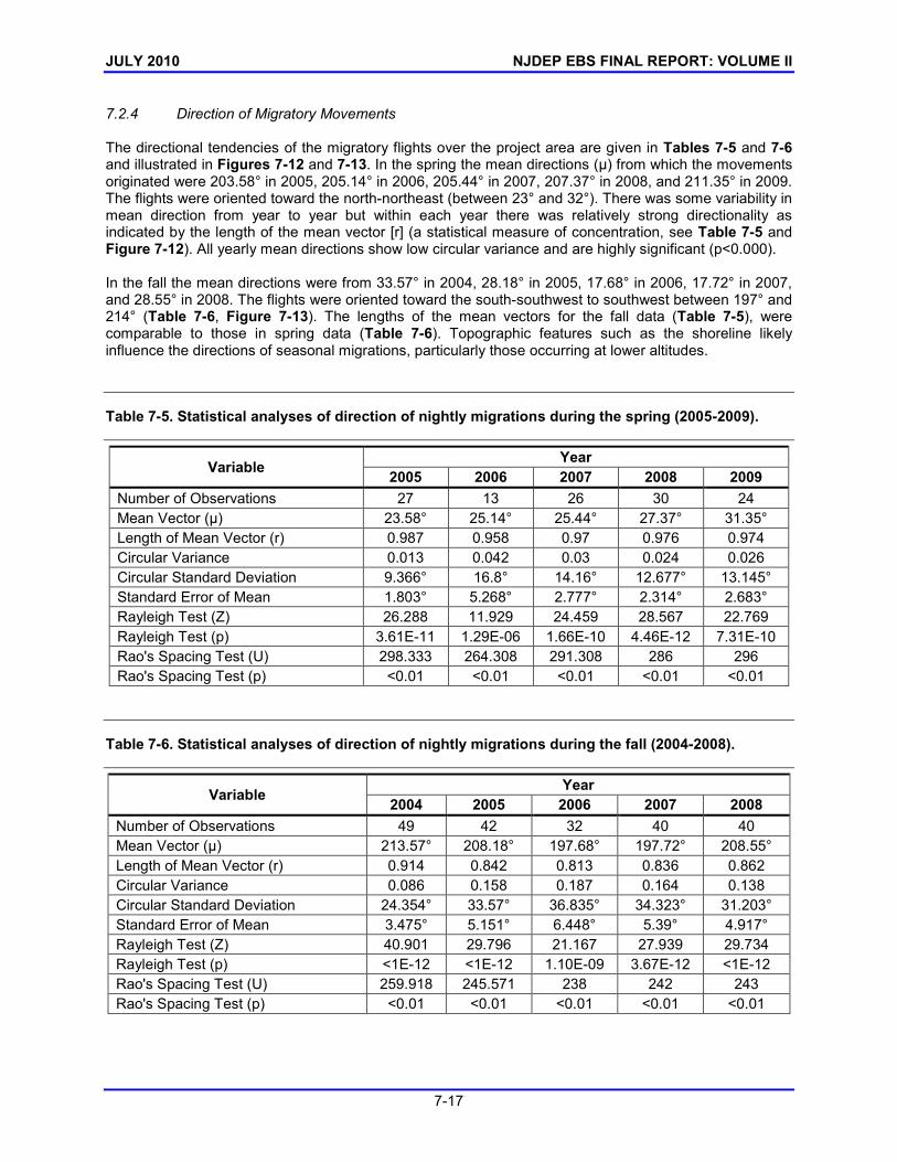
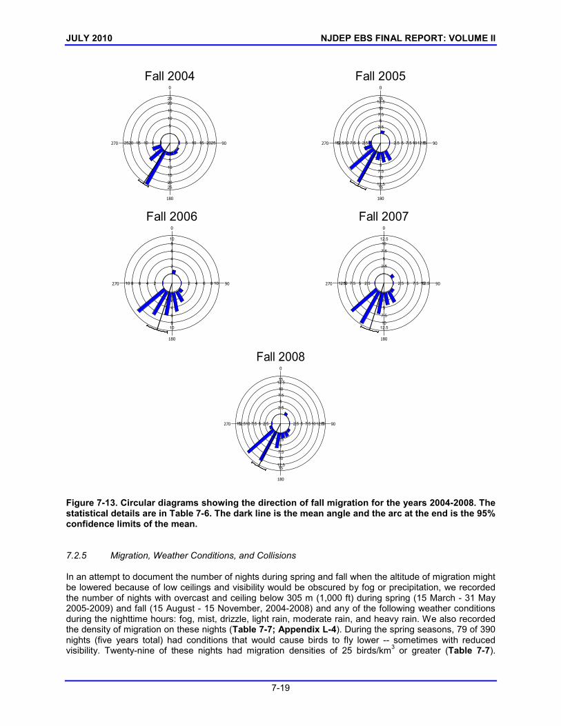
7.2.4 Direction of Migratory Movements The directional tendencies of the migratory flights over the project area are given in Tables 7-5 and 7-6 and illustrated in Figures 7-12 and 7-13. In the spring the mean directions (μ) from which the movements originated were 203.58° in 2005, 205.14° in 2006, 205.44° in 2007, 207.37° in 2008, and 211.35° in 2009. The flights were oriented toward the north-northeast (between 23° and 32°). There was some variability in mean direction from year to year but within each year there was relatively strong directionality as indicated by the length of the mean vector [r] (a statistical measure of concentration, see Table 7-5 and Figure 7-12). All yearly mean directions show low circular variance and are highly significant (p<0.000). In the fall the mean directions were from 33.57° in 2004, 28.18° in 2005, 17.68° in 2006, 17.72° in 2007, and 28.55° in 2008. The flights were oriented toward the south-southwest to southwest between 197° and 214° (Table 7-6, Figure 7-13). The lengths of the mean vectors for the fall data (Table 7-5), were comparable to those in spring data (Table 7-6). Topographic features such as the shoreline likely influence the directions of seasonal migrations, particularly those occurring at lower altitudes. Table 7-5. Statistical analyses of direction of nightly migrations during the spring (2005-2009).

Variable Year 2005 2006 2007 2008 2009

Number of Observations 27 13 26 30 24 Mean Vector (µ) 23.58° 25.14° 25.44° 27.37° 31.35° Length of Mean Vector (r) 0.987 0.958 0.97 0.976 0.974 Circular Variance 0.013 0.042 0.03 0.024 0.026 Circular Standard Deviation 9.366° 16.8° 14.16° 12.677° 13.145° Standard Error of Mean 1.803° 5.268° 2.777° 2.314° 2.683° Rayleigh Test (Z) 26.288 11.929 24.459 28.567 22.769 Rayleigh Test (p) 3.61E-11 1.29E-06 1.66E-10 4.46E-12 7.31E-10 Rao's Spacing Test (U) 298.333 264.308 291.308 286 296 Rao's Spacing Test (p) <0.01 <0.01 <0.01 <0.01 <0.01

Table 7-6. Statistical analyses of direction of nightly migrations during the fall (2004-2008).

Variable Year 2004 2005 2006 2007 2008

Number of Observations 49 42 32 40 40 Mean Vector (µ) 213.57° 208.18° 197.68° 197.72° 208.55° Length of Mean Vector (r) 0.914 0.842 0.813 0.836 0.862 Circular Variance 0.086 0.158 0.187 0.164 0.138 Circular Standard Deviation 24.354° 33.57° 36.835° 34.323° 31.203° Standard Error of Mean 3.475° 5.151° 6.448° 5.39° 4.917° Rayleigh Test (Z) 40.901 29.796 21.167 27.939 29.734 Rayleigh Test (p) <1E-12 <1E-12 1.10E-09 3.67E-12 <1E-12 Rao's Spacing Test (U) 259.918 245.571 238 242 243 Rao's Spacing Test (p) <0.01 <0.01 <0.01 <0.01 <0.01


7-18

Spring 2005

20 20

20

20

15 15

15

15

10 10

10

10

5 5

5

5

0

90

180

270

Spring 2006

8 8

8

8

6 6

6

6

4 4

4

4

2 2

2

2

0

90

180

270

Spring 2007

15 15

15

15

12.5 12.5

12.5

12.5

10 10

10

10

7.5 7.5

7.5

7.5

5 5

5

5

2.5 2.5

2.5

2.5

0

90

180

270

Spring 2008

25 25

25

25

20 20

20

20

15 15

15

15

10 10

10

10

5 5

5

5

0

90

180

270

Spring 2009

10 10

10

10

7.5 7.5

7.5

7.5

5 5

5

5

2.5 2.5

2.5

2.5

0

90

180

270

Figure 7-12. Circular diagrams showing the direction of spring migration for the years 2005-2009. The statistical details are in Table 7-5. The dark line is the mean angle and the arc at the end is the 95% confidence limits of the mean.


7-19

Fall 2004

25 25

25

25

20 20

20

20

15 15

15

15

10 10

10

10

5 5

5

5

0

90

180

270

Fall 2005

15 15

15

15

12.5 12.5

12.5

12.5

10 10

10

10

7.5 7.5

7.5

7.5

5 5

5

5

2.5 2.5

2.5

2.5

0

90

180

270

Fall 2006

10 10

10

10

8 8

8

8

6 6

6

6

4 4

4

4

2 2

2

2

0

90

180

270

Fall 2007

12.5 12.5

12.5

12.5

10 10

10

10

7.5 7.5

7.5

7.5

5 5

5

5

2.5 2.5

2.5

2.5

0

90

180

270

Fall 2008

15 15

15

15

12.5 12.5

12.5

12.5

10 10

10

10

7.5 7.5

7.5

7.5

5 5

5

5

2.5 2.5

2.5

2.5

0

90

180

270

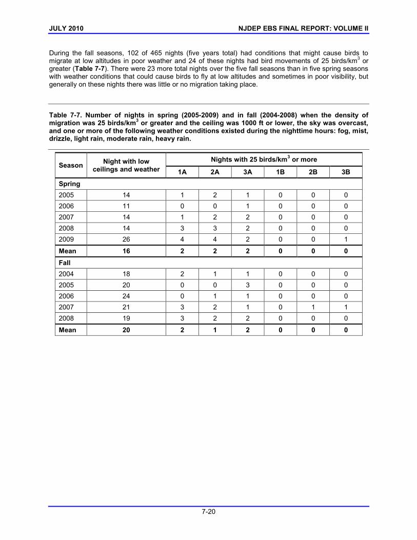
Figure 7-13. Circular diagrams showing the direction of fall migration for the years 2004-2008. The statistical details are in Table 7-6. The dark line is the mean angle and the arc at the end is the 95% confidence limits of the mean. 7.2.5 Migration, Weather Conditions, and Collisions In an attempt to document the number of nights during spring and fall when the altitude of migration might be lowered because of low ceilings and visibility would be obscured by fog or precipitation, we recorded the number of nights with overcast and ceiling below 305 m (1,000 ft) during spring (15 March - 31 May 2005-2009) and fall (15 August - 15 November, 2004-2008) and any of the following weather conditions during the nighttime hours: fog, mist, drizzle, light rain, moderate rain, and heavy rain. We also recorded the density of migration on these nights (Table 7-7; Appendix L-4). During the spring seasons, 79 of 390 nights (five years total) had conditions that would cause birds to fly lower -- sometimes with reduced visibility. Twenty-nine of these nights had migration densities of 25 birds/km3 or greater (Table 7-7).


7-20

During the fall seasons, 102 of 465 nights (five years total) had conditions that might cause birds to migrate at low altitudes in poor weather and 24 of these nights had bird movements of 25 birds/km3 or greater (Table 7-7). There were 23 more total nights over the five fall seasons than in five spring seasons with weather conditions that could cause birds to fly at low altitudes and sometimes in poor visibility, but generally on these nights there was little or no migration taking place. Table 7-7. Number of nights in spring (2005-2009) and in fall (2004-2008) when the density of migration was 25 birds/km3 or greater and the ceiling was 1000 ft or lower, the sky was overcast, and one or more of the following weather conditions existed during the nighttime hours: fog, mist, drizzle, light rain, moderate rain, heavy rain.

Season Night with low ceilings and weather

Nights with 25 birds/km3 or more

1A 2A 3A 1B 2B 3B

Spring 2005 14 1 2 1 0 0 0 2006 11 0 0 1 0 0 0 2007 14 1 2 2 0 0 0 2008 14 3 3 2 0 0 0 2009 26 4 4 2 0 0 1

Mean 16 2 2 2 0 0 0

Fall 2004 18 2 1 1 0 0 0 2005 20 0 0 3 0 0 0 2006 24 0 1 1 0 0 0 2007 21 3 2 1 0 1 1 2008 19 3 2 2 0 0 0

Mean 20 2 1 2 0 0 0

july 2010 njdep ebs final report: volume ii 7.0 … 7.pdf · july 2010 njdep ebs final report:...

Documents