journal of polish cimac
TRANSCRIPT

GDANSK UNIVERSITY OF TECHNOLOGY FACULTY OF OCEAN ENGINEERING AND SHIP TECHNOLOGY
SECTION OF TRANSPORT TECHNICAL MEANS OF TRANSPORT COMMITEE OF POLISH ACADEMY OF SCIENCES
UTILITY FOUNDATIONS SECTION OF MECHANICAL ENGINEERING COMMITTEE OF POLISH ACADEMY OF SCIENCE
ISSN 1231 – 3998ISBN 83 – 900666 – 2 – 9
Journal of
POLISH CIMAC
ENERGETIC ASPECTS
Vol. 6 No. 1
Gdansk, 2011
Science publication of Editorial Advisory Board of POLISH CIMAC


Editor in Chief: Jerzy Girtler Editorial Office Secretary: Jacek Rudnicki
Editorial Advisory Board
J. Girtler (President) - Gdansk University of Technology L. Piaseczny (Vice President) - Naval Academy of Gdynia A. Adamkiewicz - Maritime Academy of Szczecin J. Adamczyk - University of Mining and Metallurgy of Krakow J. Błachnio - Air Force Institute of Technology C. Behrendt - Maritime Academy of Szczecin P. Bielawski - Maritime Academy of Szczecin T. Chmielniak - Silesian Technical University R. Cwilewicz - Maritime Academy of Gdynia T. Dąbrowski - WAT Military University of Technology Z. Domachowski - Gdansk University of Technology C. Dymarski - Gdansk University of Technology M. Dzida - Gdansk University of Technology J. Gardulski - Silesian University of Technology J. Gronowicz - Maritime University of Szczecin V. Hlavna - University of Žilina, Slovak Republic M. Idzior - Poznan University of Technology A. Iskra - Poznan University of Technology A. Jankowski – President of KONES J. Jaźwiński - Air Force Institute of Technology R. Jedliński - Bydgoszcz University of Technology and Agriculture J. Kiciński - President of SEF MEC PAS, member of MEC O. Klyus - Maritime Academy of Szczecin Z. Korczewski - Gdansk University of Technology K. Kosowski - Gdansk University of Technology L. Ignatiewicz Kowalczuk - Baltic State Maritime Academy in Kaliningrad J. Lewitowicz - Air Force Institute of Technology K. Lejda - Rzeszow University of Technology
J. Macek - Czech Technical University in Prague Z. Matuszak - Maritime Academy of Szczecin J. Merkisz - Poznan Unversity of Technology R. Michalski - Olsztyn Warmia-Mazurian University A. Niewczas - Lublin University of Technology Y. Ohta - Nagoya Institute of Technology M. Orkisz - Rzeszow University of Technology S. Radkowski - President of the Board of PTDT Y. Sato - National Traffic Safety and Environment Laboratory, Japan M. Sobieszczański - Bielsko-Biala Technology-Humanistic Academy A. Soudarev - Russian Academy of Engineering Sciences Z. Stelmasiak - Bielsko-Biala Technology-Humanistic Academy M. Ślęzak - Ministry of Scientific Research and Information Technology W. Tarełko - Maritime Academy of Gdynia W. Wasilewicz Szczagin - Kaliningrad State Technology Institute F. Tomaszewski - Poznan University of Technology J. Wajand - Lodz University of Technology W. Wawrzyński - Warsaw University of Technology E. Wiederuh - Fachhochschule Giessen Friedberg M. Wyszyński - The University of Birmingham, United Kingdom S. Żmudzki - West Pomeranian University of Technology in Szczecin B. Żółtowski - Bydgoszcz University of Technology and Life Sciences J. Żurek - Air Force Institute of Technology
Editorial Office:
GDANSK UNIVERSITY OF TECHNOLOGY Faculty of Ocean Engineering and Ship Technology
Department of Ship Power Plants G. Narutowicza 11/12 80-233 GDANSK POLAND
tel. +48 58 347 29 73, e – mail: [email protected]
www.polishcimac.pl
This journal is devoted to designing of diesel engines, gas turbines and ships’ power transmission systems containing these engines and also machines and other appliances necessary to keep these engines in movement with special regard to their energetic and pro-ecological properties and also their durability, reliability, diagnostics and safety of their work and operation of diesel engines, gas turbines and also machines and other appliances necessary to keep these engines in movement with special regard to their energetic and pro-ecological properties, their durability, reliability, diagnostics and safety of their work, and, above all, rational (and optimal) control of the processes of their operation and specially rational service works (including control and diagnosing systems), analysing of properties and treatment of liquid fuels and lubricating oils, etc.
All papers have been reviewed @Copyright by Faculty of Ocean Engineering and Ship Technology Gdansk University of Technology
All rights reserved ISSN 1231 – 3998
ISBN 83 – 900666 – 2 – 9
Printed in Poland


CONTENTS
AdamkiewiczA., Drzewieniecki J.: OPERATIONAL PROBLEMS IN MARINE DIESEL ENGINES SWITCHING ON LOW SULFUR FUELS BEFORE ENTERING THE EMISSION CONTROLLED AREAS ……………………………………………………………. 7
Bocheński D.: ANALYSIS OF CHANGEABILITY OF OPERATIONAL LOADS OF MAIN ENGINES ON DREDGERS………………………………………………………………………… 17
Cwilewicz R., Górski Z.: PROPOSAL OF ECOLOGICAL PROPULSION PLANT FOR LNG CARRIERS SUPPLYING LIQUEFIED NATURAL GAS TO ŚWINOUJŚCIE TERMINAL ……………………………………………………………………… 25
Dymarski C., Zagórski M.: A NEW DESIGN OF THE PODED AZIMUTH THRUSTER FOR A DIESEL-HYDRAULIC PROPULSION SYSTEM OF A SMALL VESSEL …. 33
Dzida M., Olszewski W.: THE SYSTEM COMBINED OF LOW-SPEED MARINE DIESEL ENGINE AND STEAM TURBINE IN SHIP PROPULSION APPLICATIONS .…… 43
Ghaemi Hossein M.: CHANGING THE SHIP PROPULSION SYSTEM PERFORMANCES INDUCED BY VARIATION IN REACTION DEGREE OF TURBOCHARGER TURBINE ..……………………………………………………………………………………………… 55
Górski Z., Giernalczyk M.: ENERGETIC PLANTS OF CONTAINER SHIPS AND THEIR DEVELOPMENT TRENDS ……………………………………………………………………….. 71
Girtler J.: THE METHOD FOR DETERMINING THE THEORETICAL OPERATION OF SHIP DIESEL ENGINES IN TERMS OF ENERGY AND ASSESSMENT OF THE REAL OPERATION OF SUCH ENGINES, INCLUDING INDICATORS OF THEIR PERFORMANCE …………………………………………………………………………………….. 79
Girtler J.: VALUATION METHOD FOR OPERATION OF CRANKSHAFT-PISTON ASSEMBLY IN COMBUSTION ENGINES IN ENERGY APPROACH ……………… 89
Labeckas G., Slavinskas S.: PERFORMANCE AND EMISSION CHARACTERISTICS OF THE DIESEL ENGINE OPERATING ON THREE-COMPONENT FUEL …………… 99
Kniaziewicz T., Piaseczny L.: USING INFORMATION FROM AIS SYSTEM IN THE MODELLING OF EXHAUSTS COMPONENTS FROM MARINE MAIN DIESEL ENGINES ……………………………………………………………………………………………….. 109
Knopik L.: MIXTURE OF DISTRIBUTIONS AS A LIFETIME DISTRIBUTION OF A BUS ENGINE …………………………………………………………………………………………………. 119
Ligaj B.: SELECTED PROBLEMS OF SERVICE LOAD ANALYSIS OF MACHINE COMPONENTS ……………………………………………………………………………………… 125
Głomski P., Michalski R.: PROBLEMS WITH DETEMINATION OF EVAPORATION RATE AND PROPERTIES OF BOIL-OFF GAS ON BOARD LNG CARRIERS …… 133
Głomski P., Michalski R.: SELECTED PROBLEMS OF BOIL-OFF GAS UTILIZATION ON LNG CARRIERS ………………………………………………………………………………………. 141
Mielech J., Zeńczak W.: THE EVALUATION OF THE CHANGES IN THE EMISSION OF TOXIC COMPOUNDS RESULTING FROM THE POWER SUPPLY FOR THE SHIPS IN PORTS EFFECTED BY MEANS OF THE SHORE POWER ………………. 149

Rosłanowski J.: TEMPERATURE AS SYMPTOM OF THERMAL PERFORMANCE IN PISTON-CONNECTING ROD CORRECTNESS OF COMBUSTION ENGINE ….. 155
Rosłanowski J.: IDENTIFICATION OF TECHNICAL STATE OF FUEL ENGINE APPARATUS ON THE GROUNDS OF MECHANICAL OPERATION SPEED IN PISTON-CONNECTING ROD SYSTEM ……………………………………………………… 163
Rudnicki J.: ANALYSIS AND EVALUATION OF THE WORKING CYCLE OF THE DIESEL ENGINE …………………………………………………………………………………………………. 171
Stelmasiak Z.: POSSIBILITY OF IMPROVEMENT OF SOME PARAMETERS OF DUAL FUEL CI ENGINE BY PILOT DOSE DIVISION …………………………………………….. 181
Szelangiewicz T., Żelazny K.: INFLUENCE OF THE SERVICE MARGIN OF SERVICE PARAMETERS OF TRANSPORT SHIP PROPULSION SYSTEM. PROPULSION ENGINE SERVICE PARAMETERS OF TRANSPORT SHIP SAILING ON A GIVEN SHIPPING ROUTE ………………………………………………………………….... 191
Szelangiewicz T., Żelazny K.: INFLUENCE OF THE SERVICE MARGIN OF SERVICE PARAMETERS OF TRANSPORT SHIP PROPULSION SYSTEM. SCREW PROPELLER SERVICE PARAMETERS OF TRANSPORT SHIP SAILING ON A GIVEN SHIPPING ROUTE ……………………………………………………………………. 201
Zachwieja J., Holka H.: THE EFFECTIVENESS OF RIGID ROTOR’S BALANCE WITH RESONANT EXTORTION OF THE SYSTEM WITH SMALL DAMPING …………. 211

OPERATIONAL PROBLEMS IN MARINE DIESEL ENGINES SWITCHING ON LOW SULFUR FUELS BEFORE ENTERING THE EMISSION
CONTROLLED AREAS
Andrzej Adamkiewicz Jan Drzewieniecki
Maritime University of Szczecin Department of Condition Monitoring & Maintenance of Machinery
ul. Podgórna 52/53, 70-205 Szczecintel.: +48 91 4338123, fax: +48 91 4318542
e-mail: [email protected], [email protected]
Abstract
Introduction of rules connected with implementation of Sulfur Emission Control Areas and changes in MARPOL Convention Annex VI not only increased the operation costs or forced ship owners to comply with convention but first of all put pressure and provided influence on ship’s operation. In this article there are presented operational problems in Marine Diesel Engines switching from the residual fuels HFO to low sulfur residual LSFO and distillate LSGO fuels before entering Emission Control Areas (ECAs). There are defined ECA Zones in Europe and North America. There are introduced changes in limits with regards to Sulfur content in fuel oils during last years, planed trends and changes. There are characterized the changing over process, the applied procedures and methods of time calculation in changing over from HFO into LSFO/ LSGO. Besides, there are described the method of sulfur calculation in fuel during blending both grades of fuel. To conclude authors have characterized technical and legislative demands that the ship-owners have to face up to adopt the operated vessels to meet ECAs requirements.
Keywords: Emission Control Areas, SOx reduction, marine diesel engine, low sulfur fuels, fuel change over operation
1. Introduction
In response to the desire of some countries to reduce the harmful effects of ship emissions on air quality with a focus mostly on the release of sulfur oxide (SOx) and presently on nitrogen oxide (NOx) compounds and particulate matter (PM), the International Maritime Organization (IMO) Regulation 14 of Annex VI to the International Convention on the Prevention of Pollution from Ships (MARPOL) permits the establishment of SOx Emission Control Areas (SECAs), 19 May 2005 [11]. The IMO has approved two such areas: the Baltic Sea 19 May 2006 and the North Sea with English Channel 21 Nov 2007, fig. 1a. The United States and Canadian Government have requested that the IMO designate an area off their coastal waters to 200NM, fig. 1b. The US Environmental Protection Agency (EPA) is currently preparing documents for approval process and is expected to enter into force as early as August 2012 [6, 14]. In October 2008, IMO adopted stringent new standards found in Revised MARPOL Annex VI –Resolution MEPC.176 (58) to control emissions from ships [12]. The revised Regulation 14, effective 1 July 2010, adopted progressive reduction in SOx included other harmful exhaust
7

emissions from the engines that power ships as NOx and PM, and revised geographic-based standards for former SECA that was renamed as the Emission Control Area (ECA). Ships operating in designated ECAs since 1 July 2010 are required to use fuel with a sulfur content not exceeding 1.0% and from January 2015, this would be reduced to 0.1% [1, 9, 12, 14]. a) b)
Fig. 1 MARPOL Annex-VI Emission Control Area (ECA) [1, 14] a – Baltic and North Sea, b – US and Canada
European Union countries has implemented regulation relating the sulfur content of fuel used in its port under Article 4b of EU Council Directive 2005/33/EC with effective date 1 January 2010 is limited to 0.1% (replaced limits 1.5% from 11 August 2006) that applies to all types of marine fuels unless an approved emission abatement technology is employed or shore power is available. It applies to both main and auxiliary boilers [1, 9, 12, and 14].The California Air Resources Board (CARB) under its authority within the state has implemented regulations pertaining to the sulfur content limits and types of fuels can be used in Californian waters within 24NM of coastal baseline in two phases with effective date 1 July 2009, limit 0.5% and with 1 January 2012 - 0.1%. It applies to auxiliary boilers too, excluding main propulsion boilers, however low sulfur residuals fuels are not permitted only distillate fuels [1, 9, and 14].
Fig. 2 Sulfur reduction “road map” - current and future sulfur requirements for Marine Fuel Products; * - the regulation is applicable for inland waterways and at berth [14]
Current and future requirements for Marine Fuel Products used by ships in ECAs including US and Canadian countries, EU territory and CARB are presented in table, fig 2.
8

To meet the sulfur emission legislation rules is to reduce the SOx either by switching fuel supply to engine/ boiler from the Marine Residual Fuels known as HFO (Heavy Fuel Oil) into Low Sulfur: Marine Residual Fuels LSFO (Low Sulfur Fuel Oil)/ the Marine Distillate Fuels LSGO (Low Sulfur Gas Oil, ISO 8217, DMA Grade [1]) or by cleaning the exhaust gases what can be obtained in special scrubber constructions. 2. Effects of Low Sulfur Fuels on Operation of Marine Diesel Engines
Operational concerns of switching between HFO and LSFO or LSGO have the potential for several harmful effects on diesel engines as discussed in the following paragraphs. Low Sulfur (Heavy) Fuel Oils: Sulfur levels are required to be less than 1%. If LSHFO is created by a desulphurization unit, fuel aromaticity may be decreased which can result in lower fuel stability [1, 7, 9]. A consequence of this happening is increased fuel incompatibility problems when mixing with regular HFO during fuel changeover. The low sulfur processing can also lead to additional quality problems such as ignition and combustion difficulties and increased catalytic fines levels. In addition, when LSFO is carried on board for use in an ECA, it is required by MARPOL Annex VI be stored and purified separately from regular HFO. This can require piping changes to the fuel transfer and purification system. As LSFO are not applicable in some ECAs – CARB, EU Territories and after 1 Jan 2015 the sulfur limit will be 0.1% in all ECAs and if production of such an Ultra LSFO will be too expensive that they will be replaced completely by LSGO. Low Sulfur Diesel/ Gas Oils: 1. Lubricity and Low Viscosity [1, 7, 9]:
- Reduced (effectiveness as a lubricant) the film thickness between the high pressure fuel pump plunger and casing in the fuel valves leading to excessive wear and possible sticking and seizing, causing failure of these elements. This can be minimized by purchasing distillate fuels with lubricity enhancing additives and higher vis. 3 mm2/s (cSt) at 40˚C.
- Loss of capacity in fuel supply (booster) and circulation pumps due to low viscosity, fuel leaking around pump rotors, preventing the ship from achieving full power.
- Leakage of fuel through the high pressure fuel pump barrel, plunger, suction and spill valve push rods on slow speed engines. This leakage may result in a higher load indication position of the fuel rack and may require adjustment of the governor for sustained operation on low viscosity fuel or may results in worn pump’s elements (enlarged clearances). As an internal leak is part of design and is used in part to lubricate the pumping elements, it can cause too high leak rate and in consequences lead to smaller than optimal injection pressures resulting in difficulties during start and low load operation.
- Maintaining viscosity above the minimum value of 2 mm2/s (cSt) at 40˚C, fig. 3. One of the solutions is to install a fuel cooler (for tropical conditions equipped with chiller unit) that will keep the fuel temperature below 40˚C.
9

Fig. 3 Fuel temperature relation to viscosity [8]
2. Low Density: Low sulfur, low viscosity fuels typically have low density when compared to heavy fuel oils. This will result in less energy per volume of fuel (volumetric energy content) and thus will require more fuel volume to be supplied to the engine to maintain equivalent power. Engine governors and automation need to be able to adjust to the changes in fuel rack position and governor settings [1]. 3. Incompatibility of Fuels: Mixing two types of fuels can lead to risk of incompatibility betweenthem, particularly when mixing heavy fuel and low sulfur distillate fuels. If incompatibility does occur, it may result in clogging of fuel filters and separators and sticking of fuel injection pumps, all of which can lead to loss of power or even shut down of the propulsion plant, putting the ship at risk. Compatibility problems can be caused by differences in the mixed fuels’ stability reserves. If the stability level of the HFO is low there can be difficulties when mixing with more paraffinic, low sulfur fuels and as a consequence the asphaltenes can precipitate of the blend as heavy sludge, causing clogging [1, 3]. This can be minimized through on board compatibility test kits used when bunkering both HFO and low sulfur fuel called Spot Test Method for Assessing Fuel Cleanliness and Compatibility (ASTM D 4740-4) [14], by DNV Program for fuel samples send to laboratory Onboard Blending Optimization Program - BOP and Fuel Quality Test - FQS [4] or by purchasing distillate and residual fuels from the same refinery [3, 4]. If incompatibility is indicated by presence of suspended solids when equal volumes of a sample and a blend stock are mixed together there is necessity to avoid mixing these grades of fuel by discharging one grade to port facilities or more preferable to treat them by chemicals with mixing reduced to minimum in proportion maximum 80:20 [3]. The examples of the mentioned chemicals are Amergize deposit modifier/ combustion improver and Amergy222 fuel oil conditioner minimizing the effect of fuel instability and incompatibility by Drew Marine Division – Ashland’s Chemicals [5].
3. Impact of Low Sulfur Fuel on lubrication of Marine Diesel Engines
Diesel engines require lubrication in order to operate efficiently and these lubricating oils need to be compatible with fuel used in the engine. Therefore, if lube oil BN (Base Number) does not match the acidity of the fuel it will have an effect on maintaining a compatible lubricant between the fuel and the oil. Too high BN70 can develop calcium and other deposits on the liner’s surfaces. Too small BN30-50 can increase the fuel’s acidity causing additional wear on parts as well as creating problems combusting the fuel. Lube oils are used to neutralize acids formed in
10

combustion, mostly commonly sulfuric acids created from sulfur in the fuel. The quantity of acid neutralizing additives in lube oil should match the total sulfur content of the fuel. It has been established that a certain level of controlled corrosion enhances lubrication, in that the corrosion generates small “pockets” in the cylinder liner running surface from which hydrodynamic lubrication from oil in the pocket is created. In other words, controlled corrosion is important to ensure the proper tribology needed for creation of lubricating oil film, fig. 4.
a) b)
Fig. 4 Cylinder liner surface: a - ‘Open’ graphite structure with good tribological abilities from where the cylinder oil can spread, b - ‘Closed’ graphite structure with reduced tribological ability [8]
If the neutralization of the acid is too efficient (the alternative no corrosion) it can lead to bore-polishing, liner lacquering and subsequently hamper the creation of the necessary oil film resulting in increase of scuffing and accelerated wear of liner [1, 2, 8, 13]. This especially applies to slow speed engines which have cylinder lubrication and are operated continuously at high load having less need for SOx neutralizing on the liner surface due to high temperature but it can occur on trunk piston engines, too where a bore-polished liner surface hampers the functioning of oil scraper rings and leads to accelerated lube oil consumption due to access to crankcase [9]. It should be considered that irrespective of sulfur content (high or low) the fuels used in low speed engines are usually low quality heavy fuels. Therefore, the cylinder oils must have full capacity in respect of detergency and dispersancy, irrespective of the BN specified. In consequence of the above, the cylinder oil feed rate is very important factor as from one hand its consumption represents a large expenditure for engine operators but from the other hand a satisfactory piston rings/ liner wear rate and maintaining the time between overhauls is a must. To achieve these requirements engine’s producers developed high pressure electronically controlled lubricators that inject the cylinder oil into the liner at the exact position and time where the effect is optimal (MAN B&W Diesel the Alpha Lubricator System or Wärtsila RPLS Retrofit Pulse Lubrication System). Therefore, cylinder oil feed rate is readjusted depending on the actual fuel sulfur content (fig. 5) and the actual condition of piston rings and liners evaluated during inspection through scavenge ports. The practical approach for the correlation between fuel sulfur and cylinder oil can be shown as follows:
- Fuel sulfur level <1%: BN40/50 is recommended; - Fuel sulfur level 1-1.5%: BN40/50 is recommended, however BN70 can be used only
when operating for less than 2 weeks; - Fuel sulfur level >1.5%: BN70 is recommended, however BN40/50 can be used with
higher feed rate. Some ship owners supply vessels with low speed engines with cylinder oil BN50 and HFO bunker up to 3.5% of sulfur limit as company policy [4]. At present, additional researches have been conducted by several oil companies to create lubricating oil that would be compatible with different type of fuel [15].
11

Fig. 5 Cylinder oil feed rate dependent on BN40 vs. BN70 cylinder oil use [8]
4. Procedures of Changing over from HFO to LSFO/ LSGO and Methods to Assume Sulfur Content of Fuel Oil in a Mixed State
It is the responsibility of the ship-owner to ensure that it can be demonstrated, to the satisfaction of any relevant administrative body (for example Port State Control - PSC), that the fuel oil being burned within ECA complies with MARPOL Annex VI, Regulation 14 [12]. Details of fuel oil change-over procedures from HFO to LSFO/LSGO and vice versa have to be recorded in suitable log books as the Engine Room Log Book, the Oil Record Book Part 1 and a dedicated MARPOL Annex VI log book. Log Book entries could be as follows:
Arrival at/ Departure from ECA on completion/ commencement of fuel change-over. 1. Date and time of completion/ commencement of fuel change-over. 2. Position, latitude and longitude at completion/ commencement of fuel change-over. 3. Volume of LSFO/ LSGO in each tank on completion of fuel change-over. 4. Signature of responsible Officer (Chief Engineer and confirmed by Captain).
Besides, the records and history of BDNs (Bunker Delivery Note) for 3 years and MARPOL Samples for 1 year have to be maintained in ship’s custody to immediate access [4]. In addition to the mentioned above obligatory documents, as a service to ship-owners wanting documentary proof they operate in compliance with the regulations the following are available:
1. Classification Societies (CS) as ABS are prepared to issue Statement of Fact (SOF) Certificate. These will require survey by CS Surveyor to verify that vessel has dedicated low sulfur fuel storage tank, fuel piping systems suitable for its use that maintain segregation from other fuels and has operational procedures in hand for its use [1].
2. DNV Petroleum Services has developed a service where in-system samples before and upon completion of change-over can be taken and submitted for testing to determine whether complete change-over has been achieved [4].
3. Next DNVPS invention is the Blend Optimization Program (BOP) which by submitting a representative sample of each blend component will undertake fuel quality and compatibility check of the blends, calculation of the resultant blend viscosity or recommendation on optimum blend composition to meet engine fuel specification and correct injection temperature [4].
12

Fuel change-over operation should be carried out in safe navigation area and followed with ship-owner’s On Board Procedure (OBP) approved checklist. After completion Main Engine (M/E) start should be confirmed on LSGO as the increased start index might be required what can be combined with regular M/E test astern. Suggested routine for change-over from HFO to LSFO could be as follows:
- Switch off auto-start of fuel oil transfer pump. - Allow settling tank to reduce to minimum level by normal purification. Stop fuel oil
purifier. The remaining HFO quantity should allow obtaining mixing ratio below 20:80 but if the system permits it can be dropped to the overflow tank to speed the process.
- Transfer HFO from overflow tank to HFO bunker tank. - Change-over fuel oil transfer pump suction to LSFO bunker tank and refill settling tank. - Allow service tank to reduce to a minimum acceptable level by normal main and auxiliary
engine consumptions including boiler. Preferable mixing ratio 20:80. Care should be taken to allow for any vessel movement that might affect suction.
- Start fuel oil purifier. - Switch on auto-start of fuel oil transfer pump.
Suggested routine for change-over from HFO to LSGO during sailing could be as follows: - Stop FO Purifier and steam to HFO Service tank to reduce temperature to 80˚C (it will be
required in reverse process as mixing hot HFO into relatively cold LSGO can be difficult due to the mixed fuel is not homogeneous immediately and some temperature/ viscosity fluctuations are expected).
- Reduce the engine load to 25-40% to ensure a slow reduction of the temperature gradient (35-45 minutes) - The load can be changed to a higher level based on experience.
- Stop steam tracing and steam to pre-heater. - Carry out change-over of fuel by swinging 3-way valve when the fuel temperature starts to
drop not exceeding viscosity 20 mm2/s (cSt). - As a complete change-over may take several hours depending on the engine load, volume
of fuel in the circulating circuit and the system layout, observations of the temperature/viscosity must be the factor for manually taking over the control of the steam valve to protect the fuel components although in general the viscosimeter should control the steam valve for the fuel oil heater. The viscosity must not drop below 2 mm2/s (cSt) and the rate of temperature change of the fuel inlet to the fuel pumps must not exceed 2°C/minute.
The sulfur content in fuel oil is expressed in terms of analysis value at the Laboratories are generally indicated in weight percent. When other 2 fuel oils are mixed, the assumed sulfur content can be determined by the formula below or graphs on fig.6:
Xw = X1 x W1 + X2 x W2W1 + W2 W1 + W2
where: - Xw: Assumed sulfur content of the mixed fuel oil (%) - X1, X2: Sulfur content of each fuel oil (%) - W1, W2: Weight percent of each fuel oil (%)
If it is assumed that a reduced amount of total of 90 tons of HFO with a sulfur content of 3.5% is remained in the engine room FO Settling and Service Tanks then min 180 tons of LSFO/LSGO with a sulfur content of 1.0% is required before the ship enters ECAs to the assumed sulfur contentof the mixed fuel oil in respective tanks reaches Xw = 1.5%:
Xw = 3.5% � 90 tons + 1.0% � 180 tons90 + 180 tons 90 + 180 tons
13

Fig. 6 Dilution time to reach 1.5% Sulphur in percent of the fuel oil hours contained in the blending volume [14]
If we assume further that fuel oil consumption is 90 tons per day then changing should be commenced minimum 3 days before the ship enters ECAs giving a larger margin against the controlled value that depends on the sulfur content of each component fuel oil, mixing ratio and consumption of the mixed fuel oil. For the above example from the fig. 6 graph as published by DNVPS which shows the sulfur dilution time would be 200% of the fuel oil consumption time for the quantity of HFO remaining in the settling and service tanks, plus the system pipelines at the commencement of the change-over to LSFO. It can be seen that, because of the infinite number of possible values for the sulfur contents of both HFO and LSFO/LSGO, it is not feasible to dictate a definite time for the minimum duration of the change-over period. Therefore, timing for changing over cannot be assumed by any fixed figure and it is necessary to have precise calculations and to establish an enough allowance, assuming that re-bunkering has taken place since the previous change-over. Moreover, each vessel will require to have own procedures depending on bunker condition and fuel oil system.
5. Conclusions
To meet requirements of IMO Regulation 14 of Annex VI to the International Convention on the Prevention of Pollution from Ships (MARPOL) the ship-owners have to face up the problems in operation and adaptation of fuel piping/ tank systems connected with switching of fuel supply to marine diesel engines from HFO to LSFO/ LSGO and/ or to install additional equipment as wet/ dry scrubbers to clean exhaust gases [10].
The presented in this article consideration regarding operational problems in marine diesel engines switching on low sulfur fuels before entering and operating in the emission controlled areas, allows the following conclusions and expressions to be constructed: 1. LSFO combustion doesn’t give rise to any difficulties except compatibility which can be
reduced to minimum if proper rules are followed as fuel testing and mixing of two different grades in maximum 80:20 proportion. However, certain amount of chemicals (10% of bunker being mixed) should be maintained on board all the time to suspend heavy fuel particles and disperse sludge, to dissolve existing sludge, to enable the fuel to become a more stable and
14

homogeneous fluid and finally to improve combustion in case the effect of fuel instability and incompatibility occurred. Besides, one HFO bunker tank has to be separated to store only LSFO what in the most ship’s constructions and available tanks is not a problem.
2. Use of LSGO that is obligatory presently in CARB and in at internal EU waters and at berth but soon since 1 January 2015 it will cover all ECAs, causes not only compatibility problems but lubricity, low viscosity and density difficulties as well. Besides, process of switching to/ from LSGO is technically more complicated and requires marine diesel engines to be adapted to combust this fuel. As resulting from the engines producers’ analysis modern and low speed engines are well adapted to combust LSGO and with suitable protective and preventive measures and application of appropriate and the adjusted cylinder oil there is no reported problems with operation on LSGO [1, 8]. However, fuel systems will need the closer individual analysis because of quantities of LSGO required to operate in ECAs can cause that some vessels may need to be modified for additional distillate fuel storage capacity and reconstructed fuel piping including bunker lines. This condition may create some problems in transition stage and needs to be taken into consideration in advance. Next, cylinder oil can cause that some vessels may need to store two grade of oil BN70 and BN40/50 or use one grade of more universal oil BN50 considering electronically controlled feed rate and bunkering HFO with sulfur content to 3.5%. That condition mostly can be easily accomplished due to global tendency of HFO bunker deliveries and common fitting electronically controlled cylinder oil feed rate systems on low speed engines (MAN Alpha Lubrication System or Wärtsila RPLS). Even if systems are not fitted during ship’s delivery most of the ship-owners decide to install them on already operated vessels as modification during dry docking due to significantly reduced quantity of consumed cylinder oil.
3. As an alternative to using low sulfur fuel or additional supporting equipment, ship-owners may choose to equip their vessels with exhaust gas cleaning devices “scrubbers” that are bringing positive results. However, they require modifying construction already operated vessels what can be difficult especially with vessels equipped with exhaust gas economizer used for turbogenerator at sea and most of present application has testing character and require to be optimized for marine use [8, 9, and 12]. Next, considerable financial outlays to benefits in relation to use of low sulfur fuels haven’t been evaluated yet.
4. Apart of the above mentioned technical problems and difficulties with operation of marine diesel engines in ECAs, legislation demands have to be considered. It means custody of relevant documents (BDN, DNV results and sampling records), checklists, and specific manuals for each vessel, logbooks entries and crew members’ trainings.
References
[1] ABS, Fuel Switching Advisory Notice, American Bureau Survey, Houston 2010. [2] API Technical Issues Workgroup, Technical Considerations of Fuel Switching Practices,
United State Coast Guard, Marine Safety Alert, 2009. http://www.marineinvestigations.us[3] Class NK, Guidance for measures to cope with degraded marine heavy fuels, Version II,
Research Institute Nippon Kaiji Kyokai, Japan 2008. [4] DNV Petroleum Services, Fuel Quality Testing. Revision 8, DNVPS Oslo, Norway 2009. [5] Drew Marine Division, Ashland Chemicals Catalogue, New Jersey 2003. [6] EPA, Frequently asked questions about the Emission Control Area application process.
United States Environmental Protection Agency, EPA-420-F-09-001, Washington DC 2009. [7] EPA, Draft Regulatory Impact Analysis: Control of Emissions of Air Pollution from
Category 3 Marine Diesel Engines. Chapter4: Technological Feasibility, United States Environmental Protection Agency, EPA-420-D-09-002, Washington DC 2001.
15

[8] MAN Diesel & Turbo, Operation on Low –Sulfur Fuels, MAN B&W Two-stroke Engines, Copenhagen 2010.
[9] MAN Diesel & Turbo, Emission Control. MAN B&W 2-stroke Engines, Copenhagen 2010. [10] MAN Diesel & Turbo, New, Dry Scrubber Technology Proven in Field Condition. MAN
B&W Two-stroke Engines, Copenhagen 2010. [11] MARPOL, Consolidated Edition 2006, International Maritime Organization, London 2006. [12] MARPOL, Revised Annex VI, Regulations for prevention of air pollution from ships and
NOx technical code 2009 Edition, International Maritime Organization, London 2009. [13] MES, Lacquering of cylinder liner, Mitsubishi Engine Services, no. 044, Tokyo 2005. [14] Mitsui OSK Lines, Stricter low – sulfur fuel oil controls in Emission Control Area, Marine
Safety Division, Tokyo 2010. [15] Total Petrochemicals USA, Inc., Lubmarine, Talusia Universal.
http://www.lubmarine.com/lub/content/NT000F9DB2.pdf
The paper was published by financial supporting of West Pomeranian Province
16

ANALYSIS OF CHANGEABILITY OF OPERATIONAL LOADS OF MAIN ENGINES ON DREDGERS
Damian Bocheński
Gdańsk University of TechnologyUl. Narutowicza 11/12, 80-952 Gdańsk, Poland
Tel.: +48 58 3472773, fax: +48 58 3472430 e-mail: [email protected]
Abstract
This paper presents an analysis of changeability of operational loads of main engines and power consumers on dredgers of three basic types. The principles of processing measurement results, which should be used for statistical analysis of operational loads of dredger main engines and power consumers, have been formulated.
Key words: Trailing suction hopper dredgers, cutter suction dredgers, bucket ladder dredgers, main engines, main consumers
1. Introduction
Operational loads of main engines on ships are time-changeable depending on current power demand from the side of consumers driven by the engines. In the case of the main engine driving ship propeller only ( e.g. on transport ships ) load change depends on changes of : sailing speed and draught , sea and wind state , course angle , icing state of operation area, currents etc , and also on decisions as to conducting maneuvers. If main engine propells also a shaft generator then engine load changes affect also load changes of the generator. [1].
As far as technological ships are concerned the situation is more complex as their main engines drive a greater number of main consumers which are more different as to their operational characteristics. Dredgers are those of the most sophisticated type of technological ships. The number of kinds of main consumers reaches 4 and the total number of them ranges even 10. This paper presents results of the author’s own operational investigations dealing with operational loads of main engines on dredgers. Changeability of operational loads of main engines has been characterized, influence of particular kinds of main consumers on operational loads of main engines have been presented. The principles of processing measurement results, which should be used in statistical analyzing operational loads of main engines on dredgers, have been formulated.
The results have been presented for the three basic types of dredgers: trailing suction hopper dredgers, cutter suction dredgers and bucket ladder dredgers.
17

2. Main consumers on dredgers
In line with the principles given in [2] main consumers constitute different, separately driven devices intended for realization of given technological processes in accordance with a type and tasks of a dredger. The main consumers on dredgers should cover the following categories [3]: ― consumers associated with dredger’s self propelling, positioning and maneuvering (main
propellers, bow thrusters and swing winches); ― consumers associated with loosening, dredging and transporting the soil (e.g. dredge
pumps, jet pumps, cutter heads or bucket chains). Number of main consumers on a given dredger depends on the two factors:
� firstly, if the dredger is fitted with its own propelling system, � secondly, how many working operations the dredger realizes.
If a dredger is self-propelled and adjusted to realizing three working operations (i.e. loosening the spoil, lifting the output onto the dredger and transporting it to dump site) then number of kinds of main consumers equals always 4 regardless dredger type. In the case of lack of self propulsion or realizing only the two first working operations the number of kinds of main consumers is lower – equal to 2÷3. Tab. 1 shows how many and which kinds of main consumers are installed on particular types of dredgers.
Tab. 1
Kinds of main consumers which are installed on particular types of dredgers
Typesof dredgers
Kinds of main consumersNumberof kindsof main
consumers
Pro
pelle
rs
Dre
dge
pum
ps
Jet
pum
ps
Bow
and
ste
rnth
rust
ers
Cut
ter
head
Buc
ket
chai
n
Sw
ing
win
ches
Trailing suction hopper dredger X X X X - - - 4
Cutter suction dredger - X - - X - X 3Seagoing cutter suction
dreger X X - - X - X 4
Bucket ladder dredger - - - - - X X 2Seagoing bucket ladder
dredger X - - - - X X 3
Bucket ladder dredger with shore discharging installation - X - - - X X 3
3. Changeability of loads of main engines and power consumers during operations conducted within scope of dredging work
The analysis of changeability of loads of main engines and consumers was made with the use of measurement data contained in the DRAGA data base [4] and acquired a.o. in the frame of KBN research project [3]. The measuring instruments used for the measurements made it possible to perform them with 3 Hz sampling frequency. For the analysis three dredgers were selected, one of each type. They were: the trailing suction hopper dredger Inż. St. Łęgowski, the cutter suction dredger Trojan and the bucket ladder dredger Inż. T. Wenda.The selected dredgers are characterized by diesel electric drive systems of main consumers.
The only exception was the dredge pump installed on the dredger Trojan, driven by a diesel mechanical system (driven by a diesel engine through a toothed gear).
18

The service state of „ dredging work” is that characterized by the largest number of main consumers under operation, therefore during the state their influence on loads of main engines is the greatest. In Fig. 1, 2, 3 are exemplified the characteristic runs of changeable loads of main engines and consumers on the three analyzed types of dredgers working during „dredging work”. They cover about 3 hours of dredger operation.
Trailing suction hopper dredgers conduct dredging work performing in cycles the following operations: loading soil into its own hold (trailing), moving under load to a dump site, unloading (gravitational or hydraulically) as well as going back to a loading site. During dredging work all main consumers are under operation, however character of their operation is strictly dependent on operations contained in the scope of working cycle. In the basic type of power system of trailing suction hopper dredger its main engine (engines) ensures driving for all main consumers. When analyzing the load runs of main engines and main consumers driven by them attention is drawn to characteristic loads of bow thruster used during loading the soil.
The bow thrusters during loading the soil are used to positioning the dredger moving with 2÷3 kn speed. During loading the soil bow thrusters are under intermittent running. Number of their starts during the loading was in the range of 2÷20. And, duration times of single operation of bow thruster were in the range of 20÷400 sec. During hydraulically unloading character of bow thruster operation is different. Then the positioned dredger does not move. Its operation is as a rule almost continuous with 2÷6 load changes only. It should be simultaneously stressed that in favourable external conditions the bow thruster are not used at all during the hydraulically unloading. The remaining main consumers are characterized by a lower load changeability. In the case of main propellers the number of load changes during loading the output was 2÷6 , and during moving with and without output - from 6 to 12 load changes. An even smaller number of load changes concerns pumps both dredge and jet ones. In this case only 0÷3 load changes of a given pump were recorded both during loading the output and its hydraulically unloading.
If the bow thruster operation is neglected the number of load changes of main engines will be contained in the range of 11÷26 per dredging work cycle (during loading the output - 3÷10 load changes, during moving with and without output - 6÷12 load changes, and during hydraulically unloading - 1÷4 load changes of main engines). The mean value of frequency of load changes of main engines, without taking into account bow thruster operation, reached 4,86 changes per hour and was close to the mean value of load changes of main engines on fishing trawlers [1].
Suction cutter dredgers and bucket dredgers conduct dredging work with the use of swing winches, making the so called „ butterfly” bands over digging site. The loosened spoil is lifted onto a dredger and discharged to hopper barges or hydraulically transported directly to land by means of dredge pumps. During dredging work screw propellers are standing by (they are only used during free floating between works or loading sites or when going to port). Cutter heads (or bucket chains in the case of bucket dredgers), swing winches and dredge pump (pumps) on suction cutter dredgers, are always under operation. In the basic type of power system of the dredgers the dredge pump is driven by a separate
main (diesel) engine and another main engine drives the unit composed of cutter head and swing winches or bucket chain and swing winches.
Number of load changes of dredge pumps on the dredgers is very similar to that for suction hopper dredgers. On the investigated dredger Trojan it was contained within the range of 1÷3 changes per hour.
Operational loads of main consumers used for mechanical loosening the soil (cutter heads, bucket chains) are characterized by frequent changes of loads resulting from character of their work (Fig.2 and 3). The load changeability is mainly associated with the cutting- into
19

- the soil process performed by successive blades of cutter head (chain buckets ). The range of load changeability is determined by value of the coefficient minmax / NN which is the ratio of maximum and minimum loads of main consumer (where CH stands for cutter head, BC – for bucket chain).
For the cutter head the mean value of the ratio 38,2/ minmax �CHCH NN (for medium cohesive soil), and for the bucket chain the ratio 56,3/ minmax �BCBC NN (for medium cohesive soil) and
62,1/ minmax �BCBC NN (for non-cohesive soil). Similar values of the ratio are characteristic also for swing winches. Influence of changes of dredger hoeing direction on character of loads of a given main consumer is an important regularity. The influence is especially distinctly observed in the case of swing winches. a)
0
500
1000
1500
2000
2500
16:48:00 17:16:48 17:45:36 18:14:24 18:43:12 19:12:00 19:40:48 20:09:36czas
]
[kW
NSG
b)
0
200
400
600
800
1000
1200
16:48:00 17:16:48 17:45:36 18:14:24 18:43:12 19:12:00 19:40:48 20:09:36czas
]
[kW
NŚR
c)
0
200
400
600
800
1000
1200
16:48:00 17:16:48 17:45:36 18:14:24 18:43:12 19:12:00 19:40:48 20:09:36czas
][k
WN PG
d)
0
50
100
150
200
250
16:48:00 17:16:48 17:45:36 18:14:24 18:43:12 19:12:00 19:40:48 20:09:36czas
]
[kW
NPS
20

e)
0
100
200
300
400
16:48:00 17:16:48 17:45:36 18:14:24 18:43:12 19:12:00 19:40:48 20:09:36czas
]
[kW
NSS
� A �� B �� C �� D �
Fig.1. Load changeability of power system elements of the dredger Inż. S. Łęgowski; a) main engines, b) propellers, c) dredge pumps, d) jet pump, e) bow thruster; (A – trailing, B –
moving under load to a dump site, C – hydraulically unloading, D – going back to a loading site)
a)
0
20
40
60
80
17:24:00 17:45:36 18:07:12 18:28:48 18:50:24 19:12:00 19:33:36 19:55:12czas
][k
WN
GF
b)
0
5
10
15
20
25
17:24:00 17:45:36 18:07:12 18:28:48 18:50:24 19:12:00 19:33:36 19:55:12czas
]
[kW
NW
M
Fig.2. Load changeability of main consumers of the dredger Trojan; a) cutter head, b) swing winches
a)
0
50
100
150
200
250
300
16:33:36 16:48:00 17:02:24 17:16:48 17:31:12 17:45:36 18:00:00 18:14:24 18:28:48 18:43:12czas
][k
WN
ŁC
21

b)
0
5
10
15
20
25
16:33:36 16:48:00 17:02:24 17:16:48 17:31:12 17:45:36 18:00:00 18:14:24 18:28:48 18:43:12czas
]
[kW
NW
M
Fig.3. Load changeability of main consumers of the dredger Inż. T. Wenda; a) bucket chain, b) swing winches
4. Processing the results of operational measurements
Measurement instruments and methods to be applied as well as subsequent processing measurement results in order to analyze them statistically, depend on a purpose for which the operational data are collected. This author has conducted multiyear operational investigations of dredgers in order to achieve empirical data necessary for elaborating a set of novel methods of power plant design for dredgers.
From the point of view of design problems of ship power systems, are important such load changes of main engines, which lead to changes of thermal equilibrium state and are associated with distinct fuel consumption change. The thing is in the changes of a value and duration interval which can lead to a change of temperature and rate of exhaust gas as well as temperature of cooling media [1]. Starting from such premises one is able to accept that the changeability frequency of a dozen or so changes per hour at the most , i.e. changes of
duration from the range of a few up to a dozen or so minutes would be ultimate, maximum frequency of load changeability in question.
For the above mentioned reasons it is proposed to assume, for statistical analysis of distributions of operational loads of main engines and consumers on dredgers, average values of engine (consumer) loads taken from a given time interval. On the basis of the earlier presented operational data one can state that in the case of suction hopper dredgers the time interval equal to 5 minutes would be sufficient. In the case of suction cutter dredgers and bucket chain dredgers such time interval would be that of making the „butterfly” band. The time interval of making the „butterfly” band by suction cutter dredgers reaches a few up to a dozen or so minutes at the most, and somewhat longer - by bucket dredgers.
Bibliography
[1] Balcerski A.: Modele probabilistyczne w teorii projektowania i eksploatacji spalinowych siłowni okrętowych. Wydawnictwo Fundacji Promocji Przemysłu Okrętowego i Gospodarki Morskiej, Gdańsk 2007
[2] Balcerski A., Bocheński D.: Propozycja nowej struktury pojęciowej związanej zokrętowym układem energetycznym. W:[Mat] XXIII Sympozjum Siłowni Okrętowych SymSO 2002. Akademia Morska, Gdynia 2002
[3] Bocheński D. (kierownik projektu) i in.: Badania identyfikacyjne energochłonności i parametrów urabiania oraz transportu urobku na wybranych pogłębiarek i refulerów.Raport końcowy projektu badawczego KBN nr 9T12C01718. Prace badawcze WOiO PG nr 8/2002/PB, Gdańsk 2002.
22

[4] Bocheński D.: Baza danych DRAGA i możliwości jej wykorzystania w projektowaniu układów energetycznych pogłębiarek. W:[Mat] XXIII Sympozjum Siłowni Okrętowych SymSO 2002. Akademia Morska, Gdynia 2002
23

24

PROPOSAL OF ECOLOGICAL PROPULSION PLANT FOR LNG CARRIERS SUPPLYING LIQUEFIED NATURAL GAS
TO ŚWINOUJŚCIE TERMINAL
Romuald Cwilewicz, Zygmunt Górski
Marine Power Plants Department Gdynia Maritime University, 83 Morska Street, 81-225 Gdynia, Poland
Tel.: +48 58 6901-324 e-mail: [email protected]
Abstract
The liquefied natural gas should be delivered to Świnoujście terminal by the biggest and the most modern ships. Ships should be operated by Polish owners. Cargo capacity of these ships is limited by depth of waterway on Świnoujście terminal entry. The largest recently built LNG carriers with cargo capacity 250000 m3 have drought about 12m which corresponds to waterway depth. The propulsion plants of such a ships should be fuelled by natural gas witch is considered to be an “ecological fuel”. The natural gas is widely used in onshore energetic plants however in marine applications the heavy fuel oil is still dominating. It is the result of problems in adaptation of marine diesel engines to burn natural gas. That is why LNG carriers should be equipped with combined propulsion plant COGES (Combined Gas Turbine and Steam Turbine Integrated Electric Drive System) made up of gas turbines burning natural gas from boiled off cargo and thermodynamically connected steam turbine. Such a propulsion plant is successfully competing in efficiency with conventional diesel engines fuelled with heavy fuel oil.
Key words: marine combined propulsion plants, natural gas as marine fuel
1. Introduction
Decision to build LNG (Liquefied Natural Gas) terminal in Świnoujście raises the question about types of LNG carries supplying liquefied natural gas to Poland. This is Polish national interest to use Polish ships operated by Polish owners. It should be the largest ships passing the water lane on Świnoujście LNG terminal entry. The largest actually built LNG carriers (cargo capacity 250000 m3) have draft 12m and can easily pas existing waterway. Analysis show that even LNG carriers with capacity 270000 m3 can call Świnoujście terminal in the future. LNG Carrier capacity 266000 m3 is shown in figure 1.
25

Fig. 1. LNG carrier Mozah owner Qatar Gas Transport CO steaming at sea
During sea transport natural gas is kept in liquid form under atmospheric pressure in temperature –163oC. One of the basic problem during transport by means of LNG carriers is heat penetration into cargo tanks and evaporation of cargo. Boiled off gas can be liquefied by special reliquefaction system and returned to cargo tanks or can be used as fuel in ship propulsion plant. As the reliquefaction systems consume big amount of energy the better way is to use the boiled off cargo as a “ecological fuel” for ship propulsion plant. However natural gas is widely used in on land power stations the heavy fuel oil still dominates in ship propulsion. After combustion heavy fuel oil exhaust gases are very harmful to environment. Small application of natural gas for ship propulsion comes from difficulties in adaptation of marine diesel engines to burn the gas. That is why LNG carriers should be turbine driven as the turbine propulsion can be easy adopted to gas burning. It should be modern propulsion system COGES (Combined Gas Turbine and Steam Turbine Integrated Electric Drive System) consisting of gas turbines fed with boiled off cargo and thermodynamically connected to them steam turbine. COGES system has high efficiency successfully competing with efficiency of traditional diesel engine propulsion fed with heavy fuel oil.
2. COGES type marine propulsion system
Suggested for ship propulsion COGES system (fig. 2) consists of two gas and one steam turboalternators. They create central electric power station, which supplies the power for ship propulsion and ship electric net. Gas turbines 1 and steam turbine 2 are thermodynamically connected to obtain high energetic efficiency. It consists on use of gas turbine exhaust gases for steam generation in waste head boilers 3. The steam is used for steam turbine drive and for heating purposes of the ship. This way a high rate of energy utilisation is obtained and the main disadvantage of gas turbines i.e. high exhaust loss is eliminated. In addition the ship is not equipped with auxiliary diesel generators since the electric power is supplied by COGES central power station. The energetic efficiency of engine room is considerably increased. Engine room fuel systems, cooling systems and lubricating systems are simplified as well as total investment expanses. Analysis [4] appoint that COGES propulsion system has many advantages comparing to other types of propulsion in particular smaller weight and dimension (up to 30% in comparison to diesel engine propulsion), low costs of overhauls and repairing, high reliability and simple operation. Components of COGES system are shown in figure 3.
26

4
4
4
7
7
5
6
6
8
8Linia elektryczna (electric line)
Para (steam)Spaliny (exhaust gases)
Woda zasilająca (feed water)
2
3 31
1
9
10 10
11
11
Fig. 2. Combined COGES type propulsion plant 1 – gas turbine; 2 – steam turbine; 3 – exhaust gas steam boiler; 4 – main alternator; 5 – main switchboard; 6 – frequency converter; 7 – azipod propulsor; 8 – transformer; 9 – heating steam
system; 10 – feed water inlet; 11 – electric power receivers
Fig. 3. An example of COGES system components a) Gas turbine Simens type SGT, b) Steam turbine Simens type SSTc) Exhaust gas heat recovery boiler Aalborg MISSIONTM WHR-GT,
Ship propulsion should be executed by modern azipod thrusters (fig. 4). Propellers 2 are driven by electric motors supplied via frequency converters are placed in horizontally rotational pods 1. Thus the high manoeuvring ability of the ship is achieved and the ship does not need classic steering gear. If the draft of the ship is 12 m it is necessary to install two azipod thrusters.
Fig. 4. Azipod thrusters ABB1 – pod, 2 – propeller, 3 – azipod rudder fin, 4 – azipod slewing gear
The space of engine rooms with traditional low speed diesel engine and COGES system is compared in figure 5. An additional cargo space 11 is to be noticed on the ship propelled by COGES system due to smaller engine room.
3
4
12
27

Fig. 4. Comparison of machinery space of LNG carrier propelled by low speed diesel engine (a) and COGES system (b)
1 – low speed diesel engine; 2 – diesel generator unit; 3 – steam boiler; 4 – propeller; 5 – rudder; 6 – gas turbine generator unit; 7 – steam turbine generator unit ;8 – condenser; 9 – azipod propulsor; 10 – exhaust gases outlet;
11 – additional cargo space
2. Rating power and efficiency of suggested ship propulsion plant
- shaft power needed for LNG carrier with capacity 250000m3 and speed 19,5 knots is [6]: Nw = (1,34571 + 0,00003091.Dn) . v3 = 37481 kW (1)where: Dn = 120000 ton - deadweight of 250000 m3 capacity LNG carrier, v= 19,5 knots - assumed ship speed,
- electric power needed by ship network during sea passage is assumed as 2000 kW,
- hence the total power of COGES central electric station turbines is:
G
el
Gfcem
wCOGES η
Nηηη
NΣN ���
� ��� kW (2)
where: Nw = 37481 kW – power needed for ship propulsion, Nel = 2000 kW – electric power needed by ship network, �em= 0,97 – main electric motors efficiency, �fc = 0,99 – frequency converters efficiency, �G = 0,97 – generators efficiency.
Table. 1. The influence of the power distribution between gas turbines and steam turbine, specific fuel consumption and effective efficiency of the COGES propulsion system driven by heavy fuel oil HFO
Power distribution between gas turbines and steam turbine NGT/NST [%] 80/20 75/25 70/30 65/35
Gas turbines rated power [kW] 2 x 16946 2 x 15887 2 x 14828 2 x 13768
Steam turbine rated power [kW] 8472 10590 12708 14828Specific HFO consumption of the COGES system [kg/kWh] 0,188 0,176 0,165 0,153
Effective efficiency of the COGES system [%] 46,7 49,8 53,4 57,5
a) b)
1
2
3
45
6
89
10
11
10
3
28

liquefied gasboiled off gas
1
23
4 5 6
8
7
7
8
9
4
23
5 6
- 163 Catmospheric pressure
o
- 110 C o
- 10 C o
30 Co
30 Co
0,2 M
0,2 MPa
Pa
25 MPa
The efficiency of COGES system depends on the rate of gas turbines exhaust gases utilisation i.e. power distribution between gas turbine and steam turbine. In modern onshore power station power distribution between gas and steam turbines is 65/35% [9]. Today it is possible to achieve in marine applications power distribution 75/25% and 70/30% in the future. Table 1 shows characteristic data of COGES propulsion system for suggested ship according to [3].
3. Natural gas fuel system of COGES type propulsion plant
Nowadays COGES propulsion systems are used on passenger cruise liners. Gas turbines are fed with gas oil. Gas turbines of LNG carrier should be fed with natural gas.
Schematic diagram of COGES propulsion plant fuel system on LNG carrier is shown in figure 5. Liquefied gas is carried in cargo tanks under atmospheric pressure in temperature –163oC.Boiled off gas is drawn from tanks by low pressure compressors 4 (discharge pressure about 0,2 MPa, gas temperature on compressor outlet about – 111,5oC) and pressed to heaters 5 where the temperature raised to about –10oC. Low pressure gas in temperature about 30oC can be used for auxiliary boiler firing. To feed gas turbines due to pressure in combustion chambers the pressure of gas should be raised in high pressure compressors 6 to 2,5 MPa and temperature about 30oC.
The rate of cargo evaporation depends on outside ambient temperature. In case to small amount of boiled off gas in cargo tanks the system can be supplied with liquefied gas by using pumps 2 and gas vaporisers 3.
Pumps and compressors of boiled off gas reliquefaction system (it is equipment of each large capacity LNG carrier) serves in fuel system. Therefore the fuel system does not any additional equipment, only additional pipe connections between cargo system and engine room are needed.
Fig. 5. Gas turbines fuel system on liquefied natural gas carrier 1 – LNG cargo tanks; 2 – liquefied gas pump; 3 – liquefied gas vaporiser; 4 – low pressure compressor; 5 – heater; 6 – high pressure compressor; 7 – gas turbine; 8 – gas turbine combustion chamber; 9 – gas
fired auxiliary steam boiler
3. Forecast of fuel consumption for suggested ship COGES propulsion system
Rated power of COGES system turboalternators covers electric power demand during sea passage as well as in remaining operation states e.g. ship manoeuvring, stopover on port roads, cargo discharging, reliquefaction system operation and regasification system operation [2]. During cargo discharging with all cargo pumps in operation the electric power demand is about 10000 kW.
29

During boiled off gas reliquefaction this is about 6500 kW. If the boiled off gas is used as propulsion fuel it decreased to 350÷1600 kW. In that case: - daily fuel consumption of gas during sea passage is:
GdCOGES = 24 * NCOGES * gCOGES=178,9 [ton/dobę], (3)where: NCOGES = �� kW – from formula (2),gCOGES = 0,176 kg/kWh – specific fuel consumption from table 1 for power distribution 75/25%,
- the amount of daily boiled of gas from (BOG) cargo tanks is about 0,1�0,2%, accepted for calculation is 0,15%, that is:
GBOG = 0,0015 * Dn = 183,8 [tons/day] (4) gdzie:
Dn = 250000 m3* 0,49 tons/m3 = 122500 tons – mass of cargo
�LNG = 0,49 tons/m3 – LNG density.
The amount of BOG covers the daily fuel consumption of COGES system during sailing at sea with full cargo loading. In case of smaller cargo evaporation rate auxiliary cargo pumps can be used and liquefied cargo can be vaporised.
- fuel requirement for to and fro trip (loading terminal – Świnoujście discharging terminal –loading terminal): Assuming the longest trip to and fro 38 days (16 days at sea in cargo condition, 16 days at sea in ballast condition, 6 days cargo operations) gas fuel requirement is about 5500 ton, which is about 4,5% of cargo capacity. The special gas fuel tanks exclusively serving for propulsion requirements are not needed. The propulsion system will use gas fuel from cargo tanks. A suitable amount of LNG cargo for return ballast trip should be left in cargo tanks.
4. Conclusions
This paper is the next in turn opinion of authors in the subject of construction LNG carriers delivering liquefied natural gas to Świnoujście terminal and type of propulsion plant for these ships. Undoubtedly advantages of COGES system fed by natural gas lean towards it use on suggested ships. The COGES system is less expensive in construction and operation as well as simple in operation and fed by natural gas recognised as “ecological fuel”. In addition increasing prices of marine fuels in the nearest future will be higher than LNG prices, which forces to discussion about the kind of LNG carriers propulsion. Authors of the paper consider obvious the necessity of construction for Poland her own LNG carrier fleet supplying gas terminal in Świnoujście.
REFERENCES
1. Górski Z., Cwilewicz R.: Proposal of turbine propulsion for a new generation liquefied natural gas carrier with a capacity of 250000 – 300000 cbm. Journal of Kones Powertrain and Transport, European Science Society of Powertrain and Transport Publication, Vol. 14, No. 2, Warsaw 2007
2. Górski Z., Cwilewicz R., Konopacki Ł., Kruk K.: Proposal of propulsion for liquefied natural gas tanker (LNG gas carrier) supplying LNG terminal in Poland. Journal of Kones Powertrain and Transport, European Science Society of Powertrain and Transport Publication, Vol. 15, No. 2, Warsaw 2008.
30

3. Górski Z., Cwilewicz R.: Turbine propulsion of seagoing vessels as the alternative for diesel engines. Joint Proceedings, No. 20 August 2007, Akademia Morska Gdynia, Hochschule Bremerhaven.
4. Górski Z., Cwilewicz R: Proposal of Ecological Propulsion for Seagoing Ships. Journal of Kones Powertrain and Transport, European Science Society of Powertrain and Transport Publication, Vol. 16, No. 3, Warsaw 2009.
5. Górski Z., Cwilewicz R., Krysiak M.: Environmentally friendly fuel system for liquefied gas carrier propelled with 45 MW main propulsion plant. Journal of Kones Powertrain and Transport, European Science Society of Powertrain and Transport Publication, Vol. 17, No. 1, Warsaw 2010.
6. Giernalczyk M., Górski Z., Kowalczyk B.: Estimation method of ship main propulsion power, onboard power station electric power and boilers capacity by means of statistics. Journal of Polish Cimac, Energetic aspects, Vol. 5, No. 1, Gdańsk 2010.
7. Gas Turbine World Performance Specifications. 8. Significant Ships of the Year 2008. A publication of the Royal Institution of Naval Architects.9. Siemens: Combined cycle power plants. www.energy.siemens/com/us/en/power-generation
The paper was published by financial supporting of West Pomeranian Province
31

32

A NEW DESIGN OF THE PODED AZIMUTH THRUSTER FOR A DIESEL-HYDRAULIC PROPULSION SYSTEM OF A SMALL VESSEL
Czesław Dymarski
Gdansk University of Technology Ul. Narutowicza11/12, 80-950 Gdańsk, Polandtel.: +48 58 347 16 08, fax: +48 58 348 63 72
e-mail: [email protected]
Marcin Zagórski
Eaton Automotive Components Sp. z o.o. Ul. 30 Stycznia, 5583-110 Tczew tel.: +48 58 53 29 318
e-mail: [email protected]
Abstract
The paper presents a comparative analysis of different kinds of ship propulsion systems with azimuth thrusters and also constructional solution of an azimuth thrusters destined for small vessel with diesel-hydraulic driving system. Characteristic feature of the thrusters is localization under the water of the main hydraulic motor which drives a fixed pitch propeller located inside a nozzle. The motor is attached to the pod which is fixed to rotatable 360 ° vertical column with nozzle. The shaft of the motor is directly coupled inside pod with propeller shaft. The column is driven by a small hydraulic motor through planetary and cylindrical gears. The thruster has been build and preliminary tested at HYDROMECH Company and now is prepared for laboratory research.
Keywords: ship propulsion systems, diesel-hydraulic driving system, hydraulic azimuth thrusters
1. Introduction Marine propulsion systems, as well as other devices and technical systems are subjected to
continuous process improvement, both in their range of design solutions, as well as the type of drive and control. At the Faculty of Ocean Engineering and Ship Technology of the Gdansk University of Technology many years researches and design works of ship systems are conducted, especially low-power. As part of this work has produced several original design solutions propulsions, including:
� Controllable pitch propellers, one of which was used on a submarine and two others on small fishing cutters [1 and 9].
� Azimuth thrusters with bevel gear in the pod and alternative-powered by an electric or ahydraulic motor placed in the hull of a ship for dual main drive of the two-segments inland passenger ship [3– 7].
� Poded azimuth thrusters with electric motors with rare earth magnets placed in the pod anddirectly connected with the propeller, and powered with photovoltaic panels. Propulsions ofthis type were used on the small boats participating in international regattas [8].
33

� Poded azimuth thrusters with hydraulic main motor placed under water and connected directly with a propeller.
The above-mentioned experience allowed undertaking the development of modern efficient propulsion system for small vessels with high demands on manoeuvrability and reliability. Following is presented an analysis of current marine propulsion systems with azimuth thrusters and new constructional solution with working description of the hydraulic poded azimuth thruster. This thruster was designed and built within conducted at the Faculty the development project NCBR: “Development project of propulsion-technological system for a fishing vessel adopted to operate in Polish economic zone”.
2. Analysis of contemporary marine propulsion systems with azimuth thrusters
The main ship propulsion systems with azimuth thrusters are now becoming popular especially with two thrusters, each with the possibility of execution complete rotation of the propeller nacelle in the horizontal plane. This is due to a number of essential advantages of such a propulsion system, the most important being:
� Very good properties of the vessel manoeuvring.� Reduced demand for space power plant room inside the ship � Elimination the need for traditional, relatively expensive and involved a lot of space,
steering systems � Possibility of using instead of a one large a few smaller higher speed engines driving,
directly or through a reduction gear, generators (diesel-electric drive) or hydraulic pumps(diesel-hydraulic drive). The larger number of independent sources of energy with the possibility of their arrangement in the separate rooms increases reliability of the propulsion system, and thus the safety of navigation also. Besides, do not require high engine room space, allowing more efficient use of valuable space on the ship, locating power plant in relatively the least attractive part of the hull bottom.
� The modular nature of the design of thrusters considerable simplifies and accelerates the construction of the vessel, equipment installation and replacement, if necessary.
It should be noted, however, that this driver with the azimuth thrusters possess a significant disadvantage relative to conventional propulsion system, especially with low-speed two-stroke engine directly connected with the propeller shaft. It is the lower efficiency resulting from of energy losses those found in the reduction gear, which must be applied here. The value of these losses depends on the type of gear.
The highest system efficiency can be achieved using a mechanical gear transmission type "Z" with a double bevel gear. However such system is not preferred because of the complexity of the design and the inability to gear ratio smooth adjustment. The second factor, in the case of a propeller with fixed pitch unable permanent job in the optimum engine speed under varying sea conditions, which can significantly reduce the efficiency of the system in the long term operation. Use of the controllable pitch propeller would solve this problem, but would significantly increase the cost and complexity of the system. These factors make this system rather less favourable in comparison to the rest of the mentioned systems.
The use of electric or hydrostatic transmission is likely to require twice the change a form of energy: in the first mechanical energy into electrical or hydraulic and next into mechanical again, which is accompanied by specific loss.
Modern electric transmissions using frequency converters are characterized by relatively high efficiency, yet allow smooth adjustment of the propeller speed while maintaining constant optimal engine speed, which is an important advantage.
34

High-pressure hydrostatic transmissions have even better features, as far as possible control and overload protection is consider, from electrical, but their efficiency is slightly lower. The work presented in [4] is a comparative analysis of two propulsion systems: diesel electric and diesel hydraulic capacity of 2 x 150 kW shows that the efficiency of the propulsion system with hydrostatic transmission was about 5% smaller. It should be noted that in the analyzed propulsion systems, there were used azimuth thrusters with bevel gear paced in the pod and driving electric or hydraulic motor located in an upright position in the hull directly above the nozzle with propeller, what can be seen in Fig 1 and Fig 2.
Selected asynchronous electric motors were, unfortunately, about 15 times heavier and larger than the high-pressure hydraulic motors, and the total weight of the diesel-electric system increased by about 58%. Also, the cost of the electric motor was about 21% greater than the hydraulic and the whole system - by about 26%.
The above discussion does not include constructional solutions with motors placed under water in a pod, although such propulsion systems, called poded systems, are now increasingly being used especially on large passenger ships such as Queen Mary 2, and on some special ships and naval vessels. However, these are usually diesel-electric propulsion systems with high
Fig. 1. View of an example arrangement of the main components of the diesel-electric propulsion system fitted withthe electric motors in vertical position [4]. Notation : 1 – electric generating set, 2 – auxiliary electric generating set, 3 – electric three-phase asynchro-nous cage motor driving the propeller, 4 – frequency converter, 5 – main switchboard, 6 – rotatable thruster, 7 – hydraulic unit for supplying hydraulic motors, 8 – hydraulic motor fitted with planetary gear to drive the mechanism rotating the column of rotatable thruster, 9 – central „outboard water – fresh water” cooler, 10 – exhaust piping with silencers
35

Fig. 2. View of an example arrangement of the main components of the diesel-hydraulic propulsion system [4]. Notation : 1- electric generating set, 2 – combustion engine, 3 – mechanical gear, 4 – the main pump unit to drive the propeller, 5 – electric generator, 6 – rotatable thruster, 7 – hydraulic motor driving the propeller, 8 – exhaust piping with silencers, 9 – hydraulic oil supplying unit, 10 – hydraulic motors to rotate the rotatable thruster around vertical axis, 11 – electric switchboard, 12 – central „outboard water – – fresh water” cooler.
power electric motors with a relatively small size, fitted with permanent magnets made of rare earth. In the U.S., there are also constructed the hydraulic poded thrusters, but less power up to several hundred kW. The hydraulic motors are specially designed with elongated shape and with small lateral dimensions.
Poded propulsion systems in addition to the aforementioned have additional advantages such as:
� Further reducing the need for power plant space inside the ship.� Smaller hull vibrations induced by the motor - propeller driving system job, and thus less
noise and greater comfort of navigation, which is extremely important especially for passenger ships.
However these systems have some drawbacks, namely: � The high cost of motor to drive the propeller with a correspondingly high power at relatively
low speeds and small lateral dimensions so that they can be installed inside the pod of the thrusters. This is especially true for electric drive, as it requires the use of high torque motors with permanent magnets made of rare earth materials, which range in the market, is very limited and usually requires execution of the order, which dramatically increases the cost. Inthe case of hydraulic drive, the motors must be a high-pressure axial piston rather with a
36

relatively small lateral dimensions, which are virtually not available in the market. They are produced only by very few manufacturers of complete equipment of this type, that is, azimuth and tunnel thrusters.
� Serious problem in the case of diesel-electric propulsion with sufficient discharge of heat generated by electric motors from a small, hard-to-access space inside the pod.
� The problem of ensuring the proper tightness of the pressure chambers and inside of the pod.In summary the following characteristics it should be noted that in the case of vessels which
are required to have high manoeuvrability, ability to work in widely differing load conditions and a high comfortable sailing advantages poded ship propulsion system are the predominant.
3. Design assumptions
As a result of previous research work on the analysis of different propulsion systems presented in [1-9] it was decided to equip, mentioned in the introduction of a small fishing vessel, of a length of about 12 m, with the diesel-hydraulic drive system consists of two azimuth thrusters with power on each propeller shaft 80 kW.
Due to the fact that the hydraulic drive enables a relatively easy adjustment of the direction and speed values assumed that the thrusters should be equipped with fixed pitch propeller, which are relatively simple in design, and therefore more reliable and less expensive than controllable pitch propeller. Furthermore, it was assumed that the propellers should be placed in the nozzles, which allows a reduction of their external diameter, and also protects the propeller blade from rope becoming caught and hitting a floating beam or ice floe.
The basic propeller regime operating at full load power should take place at a constant direction of rotation of the propeller with the possibility of changing the speed depending on the needs and marine conditions. Manoeuvring ship can achieve by changing the angular position of the column with propeller, regardless of each of the thrusters. Reversing the propeller should be possible, but in a limited range of load and used only in justified cases, for example, needs a very precise manoeuvres. This restriction is justified by different conditions of the water flow in both directions, especially through the nozzle and the resulting wide variation in the efficiency of the drive system.
Due to the lack of free space on small fishing vessel, drive system, including azimuth thrusters should be characterized by a compact modular design with relatively small dimensions and weight.
To facilitate the selection of the best possible design solution developed technical documentation of two variants of the thruster, realistic to carry in a relatively short time and an acceptable price. The first variant is based on a more popular solution consists in using the propeller drive motor located in the hull above of the vertical column and nozzle. The drive from the motor shaft is transmitted through the vertical shaft and placed inside the pod bevel gear, to the propeller shaft. In the second variant, the motor was placed under water, attached to the pod,inside which are a propeller shaft and bearings.
The both design documentations were sent to several potential producers to prepare their offersfor the two varieties of thrusters. As a result of technical analysis of both design solutions and offerings given in terms of costs and their execution was decided to perform the second of the above-mentioned variants of thrusters, it means with hydraulic motor placed under water.
The main advantage of this solution is a direct connection of the motor shaft to the propeller shaft without the need for gear, which simplifies design and improves the efficiency of the propulsion system and reduces the investment costs. Although the engine must be operated at lower speeds, and for this reason must be a little larger and more expensive, but the cost of additional bevel gear and the vertical shaft assembly would be significantly higher.
37

4. Description of structures
The design of the thruster in longitudinal section of the assembly is shown in Fig. 3 and in three-dimensional Fig. 4. A fixed pitch propeller is set on tapered journal with parallel key of the shaft 2 and secured by bearing nut 3 screwed onto the end of the shaft. In order to protect the surface of the shaft and mentioned threaded connections against water intrusion, the cap 4 was fastened with screws and sealing O-ring to the front surface of the propeller hub. The propeller shaft is set on two identical tapered roller bearings 5 in the pod 6. The tapered roller bearings pair was applied by the need to transfer lateral forces in addition to the considerable axial forces in both directions caused by the work of the screws with the ability to change the direction of its rotation. In the front journal of the shaft an axial bore with splineway with key is made, in which the shaft of the hydraulic motor of the type 7 A2FM 125 REXROTH Company is mounted. The flange of the motors body is attached to the front face of the pod with four screws. It should be noted that the external lateral outline of the pod is the square of the same geometry as the outline of the motor flange. In order to minimize the flow resistance of water flow through the nozzle, the motor is mounted in the position shown in the figures and with hydraulic pipes screened by fairwater cap, better visible in Fig. 5 and Fig. 6. The space inside the pod is closed from the back by the cover 8. In hub of the cover there are three sealing lip rings set, cooperating with the sleeve 9, which is embedded on a cylindrical journal in the middle part of the shaft. Sleeve 9 is made of stainless steel and sealed against the propeller hub by means of O-ring.
The pod 6 is flanged connected to the bottom of the rotary column 10 and the rod 11. The lower part of the column is shaped thick-walled pipe flanges ended. An additional third small flange incomplete, truncated in front and back side is a little below the top flange, and is used to attach the nozzle 12, which is shown in Fig. 5. In the figure it is visible also a second attachment point of the nozzle by means of the flat bar welded in horizontal position to the nozzle and screwed by bolts to the bottom surface of the pod. To cylindrical surface of the column 10, in the middle of its length is a rectangular connection plate 13 welded. In the plate there are three openings connecting three concentric oil channels inside the column. Three steel pipes, appling oil to the hydraulic motor 7, are welded to the flange 14, which is attached by bolts to connection plate 10. In the flange 14 there are a few small-diameter holes to allow the connection of space inside the pod and the motor with the low-pressure drain channel in the column, bypassing the two main motor supply channels. In the cylindrical sockets of the upper part of the rod 11 there are two coaxially pipes 15 and 16 of different diameters, sealed by the rings type "O", which created three separate oil channels. Two internal channels are used to power the main engine, and the channel between the column and a larger diameter pipe is used for removal of oil from leaks in the motor.
The lower part of the column 10 is connected by connector flange with the upper part of column 17, which is set in the body of the foundation 18 by means of two bearings: single-row cylindrical and double-row spherical roller. Due to the small axial loads originating only from the weight of the suspended on the column elements, a selected double-row spherical roller bearing isentirely sufficient to transfer both of these axial and transverse loads. The space inside the body 18 is protected against ingress of water with the means of three lip rings 19 cooperating with the sleeve 20 made of stainless steel, built in a similar way as in the pod. An axial hole in the top of the column is the same diameter as the lower part, so that the sizes of
38

2
3
4
5
6
7
89
101112
14
13
15
1
16
171819
20
21
22
232425
26
272829 30
Fig3. Longitudinal section of the hydraulic poded azimuth thruster
39

Fig. 4. Three-dimensional longitudinal section of the hydraulic poded azimuth thruster
three channels are identical in the both parts. In order to ensure lubrication there the radial hole is made in the wall of the column at a height above the sleeve 20 and cylindrical roller bearings, allowing the flow of returning oil through the space with the located above bearings and the gear 26.
The body of the foundation 18 located in the vertical hole the hull flange is fastened to the lower surface of the foundation plate 21. This plate of disk shape is attached with screws to a suitably prepared foundation within the vessel. To the upper surface of the plate 21 the body 22 of the thrusters slewing mechanism gear is attached. Due to the relatively low loads and low speeds used here a single-stage cylindrical gear with straight teeth with gear ratio 1:5,1. The drive of this gear is realized by means of a hydraulic motor 23 A2FM5 REXROTH company and a planetary gear type 24 REP125 TRAMEC company, with gear ratio 35, which is attached by a flange 25 to the body 22. The small cylindrical gear wheel 26 is mounted directly on the journal of the planetary gear shaft with a parallel key. The large gear wheel 27 is mounted with screws on the upper face of the upper part of the column 17. The large wheel 27 is rigidly connected to pin 28 of
40

the upper mounting oil tubes unit. This pin with suitably shaped cylindrical outer surface, the channels and rings set with the possibility of turning in the housing 29 provides to be the rotary pressure joints. The housing is closed at the top by the cover 30 and is fixed rigidly to the gear body 22. Two connectors for connection of high pressure oil pipe are welded to cylindrical outer surface of the housing 29. Third, a small oil connector is placed in the cover 30.
Fig. 5. Axonometric (with transparent fairwater cap) and central projection view of the azimuth thruster.
5. Concluding Remarks
Presented in the article design solution of the small power poded azimuth thrusters is an attempt to introduce this type of drive for small vessels. The aforementioned advantages of poded propulsion systems justify the need for research work in this subject. The principal feature and advantage of presented solutions is usage of typical hydraulic motor of wide recognized company, which although located under the water, but is easily accessible. It facilitates the control and possible replacement of the motor. It should be noted that up to now there are none of commercially available low-power hydraulic motors, which would be aligned transverse dimensions for installation in the pod. The motor which was used here is not beneficial in this regard, but according to the authors, screened by fairwater cap, as shown in Fig. 5 does not significantly interfere with the flow of the water stream to the propeller located in the nozzle. By the time the article submission the thruster was made and subjected to acceptance tests at the manufacturer. Due to the limited technical capabilities and measuring these tests were limited to checking tightness of all the oil channels and the correctness of the mechanisms at work, but without a load.
Laboratory test of the thrusters together with complete diesel-hydraulic propulsion system at full load range will be conducted at the beginning of 2012.
The thruster, whose photograph is shown in Fig. 6, was presented on 16th International Maritime Exhibition BALTEXPO - 2011 in Gdansk, where it gathered much attention, especially owners of small vessels.
41

Fig. 6. Photography of the azimuth poded thruster presented on the 16th International Maritime Exhibition BALTEXPO – 2011 in Gdansk
References
1. Dymarski Cz.: The hydraulic drive and control of the equipment of the small fishing cutter.Marine Technology Transaction, Technika Morska, Polish Academy of Sciences - Branch in Gdańsk, Marine Technology Committee. Vol. 13, 2002 r.
2. Dymarski Cz., Dąbrowski K.: Automatic control systems for ships fitted with podded propulsion drive (POD). Polish Maritime Research. Special issue 2004. S.
3. Dymarski Cz.: An azimuthing Diesel-hydraulic propulsion system for inland vessel. IVInternational Scientifically – Technical Conference EXPLO – DIESEL & GAS TURBINE ’05. Gdańsk – Miedzyzdroje – Kopenhaga, May 09 - 13, 2005 r.
4. Dymarski Cz., Rolbiecki R.: Comparative analysis of selected design variants of propulsion system for an inland waterways ship. Polish Maritime Research, No 1(47) 2006 r.
5. Dymarski Cz., Skorek G.: A design concept of main propulsion system with hydrostatic transmission gear for inland waterways ship. Polish Maritime Research, - 2006. nr S2.
6. Dymarski Cz.: Propulsion system with a hydraulic transmission for a low draught inland vessel.Marine Technology Transactions. Technika Morska. - Vol. 17, 2006.
7. Dymarski Cz.: Analysis of two design kind of propulsion for an inland vessel. Journal of POLISH CIMAC. Energetic Aspects. Vol.2, No 1. Gdansk 2007. Editorial Office: Gdansk University of Technology, Faculty of Ocean Engineering and Ship Technology.
8. Dymarski Cz., Leśniewski W.: Numerical investigations of the engine cooling system in small power vessel pod propulsion system. Polish Maritime Research. - Vol. 15, No 4(58), 2008 r.
9. Dymarski Cz.: Effective and environmental friendly propulsion system for small fishing cutter. 1st International Symposium on Fishing Vessel Energy Efficiency E-Fishing / Adrian Sarasquete - Vigo, Hiszpania, 2010.
42

THE SYSTEM COMBINED OF LOW-SPEED MARINE DIESEL ENGINE AND STEAM TURBINE IN SHIP PROPULSION APPLICATIONS
Marek Dzida, Wojciech Olszewski
Gdansk University of Technology Narutowicza str. 11/12, 80-233 Gdansk, Poland tel. +48 58 3472135, e-mail: [email protected]
Abstract
This paper presents a concept of a ship combined high-power system consisted of main piston engine and steam turbine subsystems, which make use of energy contained in exhaust gas from main piston engine. The combined system consisted of a piston combustion engine and an associated with it steam turbine subsystem, was considered. The system’s energy optimization was performed from the thermodynamic point of view only. Any technical –economical analyses were not carried out. Numerical calculations were performed for a Wartsila and MAN Diesel & Turbo low-speed diesel engine of about 50 MW output power.
Keywords: ship power plants, ship propulsion, combined system, Marine Diesel Engine, steam turbine
Nomenclature be - specific fuel oil consumption N - power Hi - enthalpy drop in the turbine p - pressurem - mass flow rate t - temperature
Indices: combi - combined system g - exhaust gas d - deaerator k - parameters in a condenserD - Diesel engine o - live steam, calculation point exh - exhaust passage ST - Steam turbine f - fuel ss - ship living purposes FW - feed water
1. Introduction
In propulsion ship systems last years there have been adopted combined systems such as gas-steam turbine systems. These systems can reach efficiency above 60% on the land. On the sea these system has been adopted on the passengers liner Millenium. But for now it is the only example of the combined system which is connected with the biggest efficiency. However these system needs more expensive fuel, such as Marine Diesel Oil. In much majority trade ships are propelled by low-speed Marine Diesel Engine, which needs relatively cheap Heave Fuel Oil. It seems that the above tendency will continue in the world’s merchant navy for the next couple of years.
The Diesel engine is still most frequently use as the main engine in marine applications. On one hand it burns the cheapest fuel (heave fuel oil), on the other it has the highest efficiency of all
43

heat engines. The exhaust gases leaving the Diesel engine contains huge energy which can be utilised in other device (engine), thus increasing the efficiency of the engine system and reducing the emission of substance to the atmosphere.
A possible solution here can be a system combined of a piston internal combustion engine and the gas and steam turbine circuit that utilises the heat contained in the exhaust gases from the Diesel engine. The leading engine in this system is the piston internal combustion engine. It seems that now, when fast container ships with transporting capacity of 8 - 12 thousand TU are entering into service, the propulsion engines require very large power, exceeding 50-80 MW. On the other hand, increasing prices of fuel and restrictive ecological limits concerning the emission of NOx and CO2 to the atmosphere provoke searching for new solutions which will increase the efficiency of the propulsion and reduce the emission of gases to the atmosphere.
The ship main engines will be large low-speed piston engines that burns heavy fuel oil. At the present, the efficiency of these engines nears to 45 – 50%. For such a large power output ranges, the exhaust gas which leaving the engine, contains huge amount of heat available for further utilisation.
In this article has been shown the comparison the combined systems which are composited with Low-Speed Diesel engine as the main engine and steam turbine which is powered by water steam from utilisation system exploited exhaust combustion heat with the piston system. This is considered the steam turbine with single-pressure system and two-pressure system for two Low-Speed Engine Wartsila company type RTA96C and MAN Diesel & Turbo company type K98MC.
2. Marine Diesel Low-Speed Engine
In this deliberation there has been taken to compare two Low-Speed Diesel Engine, which basic parameters has been shown in the Table 1.
Tab. 1 Basic ships parameters of Low-Speed Diesel Engine
Company WARTSILA MAN DIESEL & TURBO
Engine type 9RTA 96C 9K98 MC
Power kW 46 322 48 762
Ambient air temperature oC 25 25
Barometric pressure bar 1 1
Engine speed r/min 98,5 100,4
Exhaust gases mass flow kg/s 104,5 134,25
Exhaust gas temperature oC 271 232,8
Fuel Heavy Fuel Heavy Fuel
Calorific value of fuel oil kJ/kg 42 700 42 700
Fuel mass flow kg/s 2,1467 2,369
For huge power of combustion engine, in exhaust gases which drops engine, there are much amount of heat which can be utilized.
In this combined system exhaust gases from collector of exhaust Diesel engine are directed to utilisation system in which there heat gave to water steam, which feed steam turbine cycle, making additional power, Figure 1.
44

3. Ship combined system of Diesel engine – steam turbine
The cycle of steam turbine in the combined system has been adopted with Single-Pressure System and Two-Pressure System.
In system with the Single-Pressure System, Fig. 2, accepted only one preheater in steam system, deaerator element which is heated by touch steam stream taken from steam turbine loose. Additionally there has been accepted that steam stream for ship living purposes will be taken after superheater of steam system.
Fig. 1. Combined system with the Diesel main engine and the steam turbine
In system with the Two-Pressure System, Fig. 3, received two steam pressure in boiler drum, however in low pressure boiler drum saturated steam (x=1) reinforce steam turbine and steam stream is taken for ship living purposes. There has been also accepted only one regenerative preheater, deaerator element which is heated by steam stream from turbine loose.
In those both cases in steam turbine cycle there has been taken steam turbine type: condensation, which condenser is cool down by sea water.
Fig. 2. Flow Diagram of the Single-Pressure System of Steam Turbine
45

In this calculation there has been accepted that temperature of live steam in steam turbine system will be lower about 10oC than temperature of exhaust combustion from the combined system [3]. The pressure in condenser is the same in both taken engines. To calculation connected with steam stream for ship living purposes accepted for both engines the same value and the same return temperature of water stream for ship living purposes with heat box. Deaerator is boiling type (blend) in which the condensate stream from condenser is heated by steam stream loose from turbine to taken water temperature, reinforce steam system.
Fig. 3. Flow Diagram for a Two – Pressure System of Steam Turbine
4. Comparison of calculation combined cycle for low-speed combined system
The calculation of combined cycle with low-speed combined engine and steam turbine with Single-Pressure system and Two-Pressure system is effected for two types of engine Wartsila company 9RTA96C and Man Diesel & Turbo company 9K98MC, as in Table 1.
The calculation is effected for two values of feeding water temperature, the same for two types of system. In this calculations there has been searching the maximum power of steam turbine in pressure function of live steam po. The maximum power of steam turbine system also asserts the biggest efficiency of combined cycle.
On Figure 4 is shown progress of steam turbine power in the case of pressure of live steam to constant temperature of reinforce water and for cycle with Single-Pressure system or Two-Pressure system without steam stream collection on ship living purposes. From diagrams appears that Two-Pressure system for both engine provide the maximum power of steam turbine in the case of properly taken pressure of low pressure boiler drum. The extension of pressure of low pressure boiler drum decreases the power of steam turbine. In both cases the maximum steam turbine power of Single-Pressure system is lower than the maximum power of Two-Pressure system. However the optimum pressure of live steam for Single-Pressure system is lower than pressure of live steam for Two-Pressure system.
46

a)
3000
3200
3400
3600
3800
4000
0 5 10 15 20
po [bar]
NST
[kW
]
b)
1500
1700
1900
2100
2300
2500
2700
2900
0 5 10 15 20
po [bar]
NST
[kW
}
mss = 0 tFW = 100oC
Fig. 4. The power of steam turbine in function of live steam pressure for constant feed water temperature in steam turbine cycle with Single-Pressure and Two-Pressure system (without steam flow of ship living purposes)
a) Wartsila engine 9RTA96C b) MAN Diesel & Turbo engine 9K98MC ______ - single-pressure
two-pressure - - - - - pI = 2 bar . . . . . . - pI = 4 bar _ . _ . _ - pI = 6 bar
47

a)
3000
3200
3400
3600
3800
4000
0 5 10 15 20
po [bar]
NST
[kW
}
b)
1000
1200
1400
1600
1800
2000
2200
2400
2600
2800
3000
0 5 10 15 20
po [bar]
NST
[kW
}
tFW= 100 oC
Fig. 5. The power of steam turbine in function of live steam pressure for constant feed water temperature a) Wartsila engine 9RTA96C b) MAN Diesel & Turbo engine 9K98MC
mss = 0 ______ Single-Pressure System - - - - - Two-Pressure System mss = 2000 kg/h . . . . . . . Single-Pressure System _ . _ . _ Two-Pressure System
On Figure 5 shows progresses of steam turbine power in function of live steam pressure in the case without taking flow steam on ship living purposes and for flow mss = 2000 kg/h. For both engines the power of steam turbine is lower in the case taking steam mss to cycle without taking this steam. In the same time for both engines in case of taking steam stream on ship living purposes the optimum pressure of live steam in Single-Pressure and Two-Pressure system for the
48

maximum power of steam turbine is lower the in the case without taking steam mss. For Two-Pressure system the pressure in low pressure boiler drum is the same for both cases.
Diagrams in Figure 6 show dependence of steam turbine power for two feed water temperatures.
a)
2800
3000
3200
3400
3600
3800
0 5 10 15 20
po [bar]
NST
[kW
}
b)
1000
1200
1400
1600
1800
2000
2200
2400
2600
2800
0 5 10 15 20
po [bar]
NST
[kW
}
mss = 2000 kg/h
Fig. 6. The power of steam turbine in function of live steam pressure for constant steam flow in ship living purposes and for constant feed water temperature
a) Wartsila engine 9RTA96C b) MAN Diesel & Turbo engine 9K98MC tFW = 100oC ______ Single-Pressure System - - - - - Two-Pressure System
tFW = 120oC . . . . . . . Single-Pressure System _ . _ . _ Two-Pressure System
49

a)
110
120
130
140
150
160
170
180
190
0 5 10 15 20
po [bar]
t EXH
[oC
]
b)
120
130
140
150
160
170
180
190
0 5 10 15 20po [bar]
t EXH
[oC
]
Fig. 7. Changes of exhaust gases temperatures from utilisation system of combined system for mss = 2000 kg/h a) Wartsila engine 9RTA96C b) MAN Diesel & Turbo engine 9K98MC
tFW = 100oC ______ Single-Pressure System - - - - - Two-Pressure System tFW = 120oC . . . . . . . Single-Pressure System _ . _ . _ Two-Pressure System
The temperatures of exhaust gases in utilisation system of combined system for both cases of
engine is the same for Single-Pressure and Two-Pressure system no mater of than it takes steam on ship living purposes or not, Figure 7. For higher feed water temperature, with increase of live steam pressure the exhaust gases temperature for Two-Pressure system is constant. But in case of Single-Pressure system the exhaust temperature for both engines is fast growing.
50

2
3
4
5
6
7
8
0 5 10 15 20po [bar]
NST
/ ND
[%]
mss = 2000 kg/h tFW = 120oC Fig. 8. Reference of steam turbine power in function of fresh steam pressure of Single-Pressure and Two-Pressure
system Engine 9RTA96C ______ Single-Pressure system - - - - - Two-Pressure system
Engine 9K98MC . . . . . . . Single-Pressure system _ . _ . _ Two-Pressure system
120
130
140
150
160
170
180
190
0 5 10 15 20po [bar]
t EXH
[oC
]
mss = 2000 kg/h tFW = 120oC
Fig. 9. Exhaust gases temperature of utilisation system in function of live steam pressure of Single-Pressure and Two-Pressure system
Engine 9RTA96C ______ Single-Pressure system - - - - - Two-Pressure system Engine 9K98MC . . . . . . . Single-Pressure system _ . _ . _ Two-Pressure system
51

In Figure 8 shows reference power of steam turbine in the proportion to Diesel engine power in function of live steam pressure. Alike for Wartsila company engine and for MAN Diesel & Turbo company engine the power of steam turbine from Two-Pressure system is higher in the proportion to Single-Pressure system. The relative power of steam turbine with Wartsila engine is higher about 46-61% than the relative power of steam turbine in MAN Diesel & Turbo engine. The capability of temperature progress of exhaust gases from utilisation system is similar, Figure 9. For Wartsila engine the exhaust gases temperature for Single-Pressure system and Two-Pressure system are lower.
5. The parameters of steam turbine cycle for combined system
From thermodynamic calculations of steam turbine cycle for combined system there has been appointed the parameters of steam turbine for engine company: Wartsila and MAN Diesel & Turbo. It has been searching the maximum power of steam turbine for two values of feed water temperature 100 oC and 120 oC, however the calculations has been done for cycle without taking the steam flow on ship living purposes and for taking flow mss = 2000 kg/h.In Table 2 there has been shown calculations value of combined cycle for maximum power of steam turbine in accepted steam flow on ship living purposes.
Engine 9RTA96C company Wartsila The maximum power of steam turbine with Single-Pressure system is smaller than power of
steam turbine with Two-Pressure system about 7,3 % for tFW = 120oC and about 12 % for feed water temperature equal 100 oC. The power of steam turbine for higher feed water is smaller beside calculation for tFW = 120oC properly about 5,5 % for Single-Pressure system and 9,2 % for Two-Pressure system. The live steam pressure for Two-Pressure system is higher than for Single-Pressure system. For higher feed water temperature the live steam pressure is going high and is almost 3 times higher for Two-Pressure system than for Single-Pressure system. The live steam flow for Single-Pressure system is higher about 24-30 % in the proportion to Two-Pressure system, conversely is with decrease of enthalpy in steam turbine, properly is growing about 23-26 % in Two-Pressure system. The temperature of exhaust gases for Single-Pressure system is higher than for Two-Pressure system, but with the grown of tFW the temperature of exhaust gases is also going up. The flow of heating steam in Two-Single system md is higher about 12-23 % in the proportion for Single-Pressure system, which is cause by bigger flow of condenser in the condenser of Two-Pressure system (higher about 5-18 %). The calculations show steam turbine in combine system with Two-Pressure system cause the acceleration of propulsion system efficiency, decreasing specific fuel oil consumption for about 5,7-6,2 % in the proportion for classic efficiency system with low-speed Diesel engine.
Engine 9K98MC company MAN Diesel & Turbo In combined system with engine company MAN Diesel & Turbo the maximum power of steam
turbine is obtained for Two-Pressure system, but there is noticed that it is high dependence from feed water temperature. For feed water temperature 120 oC the maximum power of steam turbine is comparable for both system. With decrease of feed water temperature to 100 oC, the maximum power of steam turbine with Two-Pressure system is higher about 7% than the power of turbine with Single-Pressure system. The optimum of live steam pressure, is similar to combined system with engine company Warsila, which is also higher for Two-Pressure system (about 4 times more) in the compare to Single-Pressure system. The flow of live steam and the stream of heating steam in the deaerator is bigger for Two-Pressure system, properly about 28-38 % and 7,9-9,6 % in the compare for Single-Pressure system. The stream of condenser is smaller in Single-Pressuresystem. The temperature of exhaust gases from system for tFW = 100oC is almost exactly for both
52

system, but for tFW = 120oC the temperature of exhaust gases is higher about 10oC for Two-Pressure system than for the temperature for Single-Pressure system. The decrease of enthalpy in both cases in steam turbine is higher for Two-Pressure system beside of feed water temperature, for tFW = 100oC is about 24,5 %, and for 120oC about 30% in the proportion for Single-Pressuresystem. The delve studies show that for combined circulation with higher of feed water temperature for Single-Pressure system is comparable with Two-Pressure system in the case of steam turbine power, but for the feed water temperature is smaller (100 oC) the increase of steam turbine in Two-Pressure system is not so big in comparable to Single-Pressure system. Therefore it appears that for this engine in combined system in relative to comparative low temperature of exhaust gases from Diesel engine, the system of steam turbine should be feed from Single-Pressure system (invest cost are lower). For this case the efficiency of combined system is higher than for classic system, and also there is lower specific fuel oil consumption - about 4,8-5,1 % for tFW = 100oC and about 4,6 % for tFW = 120oC in the compare to classic Diesel engine.
Tab. 2. The calculations of combined cycle for the maximum power of steam turbine
9RTA96C Watrsila 9K98MC MAN Diesel & Turbo ND kW 46332 48762 tg oC 271 232,8
beD g/kWh 166,8 174,9 �D % 50,55 48,2
Waste Heat Boiler Waste Heat Boiler Single-Pressure Two-Pressure Single-Pressure Two-Pressure
mss kg/h 2000 tFW oC 100 to oC 261 222,8 po bar 3 10 2 6 pI bar 2 2 mo kg/h 18811 14296 19332 14016 md kg/h 2144 2634 2204 2417 mk kg/h 16666 18811 17128 17882 tEXH oC 136,8 125,3 127,2 126,3 NST kW 2765 3085 2466 2647
Ncombi/ND % 105,97 106,66 105,06 105,43 �combi % 53,56 53,91 50,64 50,82 ��/�D % 5,97 6,66 5,06 5,43 becombi kg/kWh 157,41 156,39 166,5 165,9
�be/beD % -5,63 -6,24 -4,81 -5,15 Hi kJ/kg 580,8 714,4 508 632,3
tFW oC 120 to oC 261 222,8 po bar 3 12 2 8 pI bar 3 3 mo kg/h 18811 13168 19332 12083 md kg/h 2690 3010 2687 2900 mk kg/h 16121 16930 16644 15466 tEXH oC 141,7 141,6 131 141,2 NST kW 2621 2823 2331 2333
Ncombi/ND % 105,66 106,1 104,8 104,8 �combi % 53,40 53,63 50,51 50,51 ��/�D % 5,66 6,09 4,78 4,78 becombi kg/kWh 157,9 157,2 166,9 166,9
�be/beD % -5,35 -5,74 -4,56 -4,56 Hi kJ/kg 580,8 733,2 508 663,2
53

6. Final conclusions
From the compare of combined system Diesel engine with steam turbine for two types of low-speed engine appears:
- achieved powers of steam turbine for both engine increase the total power of system from 4,8 to 6,4 % for engine 9K98MC company MAN Diesel & Turbo and 5,7-6,7 % engine 9RTA96C company Wartsila. The powers of steam turbine for engine company Wartsila is higher than for combined system with engine company MAN Diesel & Turbo. It appears that from higher heat energy tight in exhaust gases of Wartsila engine (the temperature of exhaust gases is high about 38 oC),
- combined systems with engine company Wartsila have bigger efficiency, - for engine 9RTA96C it appears that it is more profitable to use Two-Pressure system in
combined system, whereas in engine 9K98MC using Two-Pressure system do not radically increase the power of steam turbine. What more, on that content of sulphur in fuel, producers advice higher temperature of feed water, for example MAN Diesel & Turbo advices temperature of feed water no lower than 120 oC [3, 4].
It is possible to adopt combined cycle Marine Diesel Engine as major engine and steam turbine which uses heat inside exhaust gases of Diesel engine. Those systems can have thermodynamic efficiencies compare to circulations of combined gas turbines, whose are connected with steam turbines. Adopted combined system in case of variant and load of major engine can help increasing of power system from 4,8 to 6,7 % in the compare to conventional system for the same fuel flow. Therefore combined system decreases individual fuel expenditure about 4,6-6,24 % in the proportion to conventional system. The efficiency of combined system is growing in the proportion to conventional system similar to system power, i.e. from 4,8 to 6,7 % achieve efficiency values of system about 50,5-53,9 % of maximum power. Adoption of combined system not only gives thermodynamic advantages – increase of efficiency and economic – lower fuel consumption for the same power of propulsion system, but also ecologic advantages.
References
[1] Advances in Gas Turbine Technology. Chapter (Dzida M.), Possible Efficiency Increasing of Ship Propulsion and Marine Power Plant with the System Combined of Marine Diesel Engine,Gas Turbine and Steam Turbine, ISBN 978-953-307-611-9, Book edited by:Dr. Ernesto Benini., INTECH.
[2] Dzida, M., On the possible increasing of efficiency of ship power plant with the system combined of marine diesel engine, gas turbine and steam turbine at the main engine - steam turbine mode of cooperation. Polish Maritime Research, Vol. 16, No.1(59), 2009, pp. 47-52, ISSN 1233-2585.
[3] Kehlhofer, R.,Combined-Cycle Gas & Steam Turbine Power Plants, The Fairmont Press, INC., 1991,ISBN 0-88173-076-9, USA.
[4] MAN B&M.The MC Engine. Exhaust Gas Date. Waste Heat Recovery System. Total Economy, MAN B&W Publication S.A.,October 1985, Danish.
[5] MAN Diesel & Turbo & Turbo, Stationary Engine. Programme 4th edition, Branch of MAN Diesel & Turbo & Turbo SE, Germany, 2010, Available from www.mandieselturbo.com.
[6] Sulzer RTA 96C, Engine Selection and Project Manual, June 2001, Wartsila.
54

CHANGING THE SHIP PROPULSION SYSTEM PERFORMANCES INDUCED BY VARIATION IN REACTION DEGREE OF
TURBOCHARGER TURBINE
M. Hossein Ghaemi
Gdansk University of Technology ul. Narutowicza 11/12, 80-233 Gdańsk, Poland
tel.: +48 58 3486053, fax: +48 58 3486372 e-mail: [email protected]
Abstract
This paper presents a detailed mathematical model of ship propulsion system including slow speed diesel engine, screw propeller and governor. This mathematical model is then employed to investigate the system performances both in steady state and unsteady states. The simulation results are checked and the model is verified using experimental data. Next an original method for the system sensitivity analysis against changing of parameters is given. This method is finally applied for investigating the influence of degree of reaction of turbine of turbocharger on the system behaviour.
Keywords: diesel engine, ship propulsion, sensitivity, turbocharger, degree of reaction
Symbols a constant, parameter A area, auxiliary function b constant, parameter c specific heat, constant, parameter C coefficient, constant d constant, parameter D diameter, draught e constant, parameter f fuel-to-air ratio, frequency F equivalence ratio h specific enthalpy, calorific value, fuel
rack J mass moment of inertia, performance
index, advance number K parameter, coefficient l length L auxiliary function m mass, number M torque, moment n number, polytropic exponent p parameter P pressure, set of parameters Q heat, heat transfer, propeller torque r number
R gas constant, resistance, weighting matrix Re Reynolds number S sensitivity t time T temperature, time constant, thrust u specific internal energy, speed, input,
control V volume, speed, function x direction coordinator y direction coordinator z number, direction coordinator, input,
disturbance
Greek letters � coefficient, heat transfer coefficient � generalized linear matrix, displacement,
average � cooler effectiveness, insensitivity � efficiency, acceleration � adiabatic exponent, thermal conductivity � excess air coefficient (factor), canonical
variable, Lagrange multiplier � blade speed ratio, dynamic viscosity,
power angle, sensitivity coefficient
55

� pressure ratio � reaction degree of turbine, density � crank angle, function � flow function � angular velocity
Subscripts 0 initial value/condition amb ambient am air inlet manifold (receiver) av air inlet valve (or port) blr auxiliary blower B brake power c compressor clr cooler com combustion cyl cylinder cr. critical d discharge dyn dynamic e engine eq equivalent f fuel, final value/condition g exhaust gas gm exhaust gas manifold (receiver) gv exhaust gas valve (or port) G governor hr heat release hr0 start of heat release H pitch i index of cylinder number, integration
j index of cylinder number, integration l mechanical losses max. maximum min. minimum mix mixing mot motored nom. nominal opt optimum P propeller pis piston red reduced, corrected ref reference res residual gas s index of cylinder number, integration sto stoichiometric sur surrounding, surface sw swept t time, turbine, theoretical tc turbocharger W water
Abbreviations CPP Controllable Pitch Propeller FB Fuel Burnt FBR Fuel Burnt Rate FPP Fixed Pitch Propeller MCR Maximum Continuous Rating MEP Mean Effective Pressure MMEP Mechanical losses in the form of Mean
Effective Pressure TDF Thrust Deduction Factor
1. Introduction
To design and analyze a marine slow speed diesel engine and its control system it is necessary to know which parameters have considerable influence the system performance. Additionally, it should be cleared how these performances are affected by the system parameters. In other words sensitivity of the system should be analyzed. To interpret sensitivity of the system, one needs a clear criterion or set of criteria. Let’s consider only the related control system. In practice there are some defined limitations in Classification Society Rules. However, most of them take into consideration only the response of the system, which in the case of marine diesel engines control system is angular velocity of propeller or engine shaft, with no particular attention on other state variables. Perhaps the main reason is that the most known models for control system of ship propulsion system could not deliver all dynamic events of the system. Here an Instantaneous Value Model of Ship Propulsion System, which gives the main dynamic events of the system has been presented. By simulating the system, accuracy and satisfactory of the model was confirmed, when the results are compared with experimental data. Based on these results, author has found that the level of dependency of engine performances to reaction degree of turbine of turbocharger is very high. In this paper it is tried to answer how this parameter influence the system characteristic. Different criteria for parameter sensitivity are discussed and a new one is delivered.
Sensitivity question arises whenever we attempt to construct a physical system from a set of mathematical specifications. One of the goals of sensitivity analysis is to assign accuracy requirements for system parameters consistent with sensitivity significance in the system model. The utilization of sensitivity in control system design was extended in the late 50’s and early 60’s by many authors who contributed during this period by relating stability and other system
56

characteristics to system sensitivity functions. Thus, sensitivity became an important part of control system design and synthesis. It is also shown that sensitivity analysis could be a useful tool for optimum control system design.
2. Diesel engine model
The model is a zero-dimensional instantaneous quasi-steady one for a turbocharged two-stroke diesel engine. It comprises the compressor, the charge air cooler, auxiliary blowers, the scavenging air receiver, the inlet air port or valve, the cylinders, the exhaust port or valve, the exhaust receiver and the turbine.
All gases follow the law of the ideal gas. The basis of the model is to consider the multi-cylinder engine as a series of thermodynamic control volumes, linked by mass or work transfer. These control volumes are compressor, scavenging air receiver, cylinders, exhaust receiver and turbine. Heat, work and mass transfer across the boundaries of these control volumes are then calculated. The subsystems are treated as quasi-steady open thermodynamic systems. The model is that due to [1, 3, 5, 8] which themselves are developments of other studies like [7].
2.1. Compressor and inlet air system The compressor ratio is given as the ratio of the total pressures to ambient pressure:
� �ambcc PP�� , (1)
in which
dynclrblramc PPPPP ������ , (2)
20 )( ambamblrblrblr PPaPP ���� , (3)
)( ambamdyndyn PPaP �� , (4)
where P indicates pressure, superscripts am, blr, clr, dyn and amb express air inlet manifold (receiver), auxiliary blowers, charge air cooler, dynamic and ambient, respectively; and ablr, adynand Pblr0 are constants that have to be expressed based on experimental tests or characteristic of the auxiliary blowers and the compressor. Constant ablr is taken to give zero pressure rise at approximately between 40% and 50% power. At higher power levels the auxiliary blowers do not operate. The constant adyn is taken to give a typical dynamic pressure at the compressor outlet.
Charge Air Cooler: A linear relationship between pressure drop in the cooler and pressure of the scavenging air receiver has been considered:
)( ambamclrclr PPaP ��� , (5)
where aclr is a constant. Mass accumulation in the charge air cooler is modelled through the scavenging air receiver.
Compressor: The power of compressor, Nc, is
ambcccc hmhmN �� �� , (6)
where cm� is the air flow rate after compressor and ambient air enthalpy, hamb, can be calculated for
57

fresh air at ambient temperature and enthalpy of air passing the compressor, hc, should be calculated for fresh air at temperature of outlet air from the compressor:
��
�
!!
"
#���
���
!!"
# �
11
amb
amb
kk
cca
ambambc
TTT ��
. (7)
The air mass flow after compressor and compressor efficiency are functions of angular velocity of turbocharger shaft, �tc, pressure ratio, �c, ambient air temperature, Tamb and ambient air pressure, Pamb, can be illustrated using the static characteristic of the compressor.
Finally, total efficiency of the compressor �c, when the mechanical efficiency, �cm, is assumed independent from �tc and �c (and therefore constant), can be obtained:
cmcac ��� �� . (8)
2.2. Flow through valves and ports A simple one-dimensional model for flow through a valve (or port) using the analogy of an
orifice and having an equivalent flow area or scaled real flow area is used:
11
1
TRPACm vvdv ��� , (9)
where vm� is mass flow rate through the valve (or port), Av is flow area, Cd is discharge constant coefficient, �v is flow function, T is temperature, R is gas constant and subscript 1 denotes the condition of the flow at upper point.
$$$
%
$$$
&
'
())
*
+
,,
-
.��
!"#
�
/))*
+
,,-
.���
!!"
#�
��
��
�
.
2/1
11
.
2/112
;1
2
;1
2
cr
kk
crk
kk
v
kk
kk
��
����
� , (10)
where
� �12 PP�� ,1
. 12 �
��
!"#
��
kk
cr k� . (11)
k is adiabatic exponent and subscript 2 denotes the condition of the flow at lower point. The appropriate forms of equation (10) for inlet air and exhaust gas valves (or ports) are
considered. Both normal and reverse flow, i.e. from scavenging air receiver to the cylinder or reverse flow, and from the cylinder to the exhaust receiver or reverse flow have been considered in the model.
2.3. Control volumes: receivers and cylinders The scavenging air receiver, exhaust receiver and cylinders are modelled through the mass
balance and the energy balance equations. Both normal flow and reverse flow are taken into
58

account, but reverse flow through the compressor is unlikely to occur and auxiliary blowers prevent such a regime in low speeds. The possibility of reverse flow at the turbine is ignored, too.
The total volume of scavenging air receiver is modelled as the total of the volumes of charge air cooler and inlet air boxes. Exhaust pulses from the cylinders are conducted to the exhaust receiver through exhaust diffusers. Two flow regimes can be considered: normal flow from cylinders to the receiver and from the receiver to turbine, and reverse flow from any cylinder. Heat transfer from exhaust gas to the receiver surface area must be accounted, unless the receiver is very well lagged. It is assumed that the exhaust gas from cylinders is to be perfectly mixed with the contents of the exhaust receiver. The equivalence ratio in the receiver will not be constant if gas is entering from a cylinder during its scavenging or overlap period.
The basic periods occurring in the cylinders can be divided as: 1) closed cycle period, 2) blow-down period and 3) scavenging period. These processes are considered separately, and subdivided according to flow direction as normal and reverse.
Closed cycle period includes combustion process. The one-zone model for combustion is applied here. For scavenging period a two-zone model is taken into account so that the cylinder charge comprises a fresh air zone and a residual gas zone. It is considered that a part of the incoming fresh inlet air is mixed with the residual gas. The model is a compromise between pure displacement and perfect mixing. For other periods a one-zone model is applied which is closed to reality.
General equations of mass, m, and energy balance are as follows, respectively:
0��
n
i imdtdm
1, (12)
TudtdF
Fu
dtdmu
dtdVPmh
dtdQ
mdtdT
1111 11
�)*
+�,
-
.��
!"# ���� 0 0 � , (13)
where u is internal energy and V is volume. Moreover, the fuel-to-air ratio f, is related to equivalence ratio of exhaust gas F, as F=f/fsto, and fsto is the stoichiometric fuel-to-air ratio.
The derivative of the equivalence ratio, F, is:
$%
$&
'
��
���
!!"
#��
sto
fb
sto
fFFdtdmF
dtdm
fF
mF
dtdF
11
11, (14)
where
RccTu
pv ���11 , (15)
airuuFu
��11 , (16)
hence cv and cp are specific heat in constant volume and constant pressure, respectively. Therefore, the general equation of energy balance of two-zone control volume can be given as
in (17) in which the subscript 1 and 2 are used for the two distinct zones. The mass of zones are none-zero.
59

����
�
!!!!
"
#
���
�����
!!"
#��
��
!"# ��
�
21
2
222
1
11
1
1221
1
2
222
21
1
1111
111
PVPVTuTmT
umT
AdtdV
VVVPL
TuTm
dtdVPLL
dtdT
111
1
11
, (17)
where
dtdF
FR
Rdtdm
mdtdF
FR
Rdtdm
mA 2
2
2
2
2
2
1
1
1
1
1
11
111111
11
���� , (18)
iiii
i
ii
iii mh
dtdQ
dtdF
Fum
dtdmuL �00 �����
11 . (19)
A corresponding equation is derived for zone 2.
2.4. Combustion and heat release Heat release rate can be calculated based on Wiebe’s function:
))*
+
,,-
.���
!!"
#��
�����
!!"
#��
��� )1(
02
1
012
1
exp)1(K
com
hr
K
com
hr
tttK
tttKKFBR , (20)
where FBR indicates non-dimensional fuel burning, K1 is the shape factor, K2 is the combustion efficiency coefficient, thr0 illustrates time in which combustion starts, and �tcom refers to the duration of combustion. According to [5]:
3.0
,
,
5.0
11 ��
�
!!
"
#
��
�
!!
"
#
��
�
!!
"
#�
��ref
refcylz
cylzrefref m
mIDID
KK , (21)
5.06.0
��
�
!!
"
#
��
�
!!
"
#���
refrefcyl
cylrefcomcom F
Ftt
��
, (22)
where ID is ignition delay and the subscript ref, z and cyl indicate reference point, beginning of compression and cylinder in question, respectively.
Now, the rate of heat release can be easily found:
com
ff
tQ
FBRdt
dQ�
�� , (23)
.forfcomf hmQ �� , (24)
where hfor is the enthalpy of formation, �tcom is duration of combustion, mf is fuel mass and
60

�com is the energy conversion rate denoting the efficiency of combustion as follows [2]:
$%
$&
'
/�
/2�(
�
0.1;95.00.1;)(exp
;0.1
.
.
��
������
�
�
���
dbca cr
cr
com , (25)
in which � is the excess air factor, ��34F. a�5 b�5c�and d� are constants which depend on the critical smoke limit of the excess air coefficient of combustion �cr..�cr. is a constant around 1.4.
The mass of fuel injected can be defined as a function of relative fuel rack position:
fMCRff Xmm � , (26)
where mf MCR is the mass of the fuel injected when the fuel rack position is 1.0 and Xf is fuel index.
2.5. Heat transfer Hear transfer coefficient in cylinders, �cyl, is:
� �8.0
6
_
553.02.0
8.04
))*
+
,,-
.����
motcylcylrefref
refswpis
cylcyl
cylcyl PP
VPTV
KuKTD
PK� , (27)
in which K4 is selected as 0.0832. during compression and expansion and K5 and K6 are equal 2.28 and 3.24e-3, respectively. They are equal 6.18 and zero for charge renewal period, respectively. Vsw is the swept volume by the piston. Cylinder pressure of a motored engine, Pcyl mot is the
cylinder pressure with no combustion and pisu_
is the average speed of cylinder piston. Then the convective heat transfer (gas-to-wall) can be calculated:
� �surcylcylcylcyl
cyl TTAdt
dQ��� , (28)
the subscript cyl sur denotes the surface of the cylinder and the total surface area for heat transfer calculation Acyl, comprises cylinder liner, cylinder cover, exhaust valve and piston crown surface areas.
Heat transfer in exhaust gas receiver is
)*
+,-
.�
����
�
!!"
# �
surgmicylgm
gmigi
surgas TTT
Adt
dQ2
� , (29)
where dQgas-sur/dt refers to the heat transfer from exhaust gas coming from cylinder i to the exhaust receiver surface or inversely. �g is the heat transfer coefficient and subscript gm denotes gas receiver. The temperature of the exhaust gas in the model is taken as the mean value of instantaneous exhaust gas temperature from the cylinder and the average exhaust gas temperature in the receiver. The temperature of exhaust pulse can be defined as:
� � � �� � � �$%
$&'
6
��
0;
0;
irescylirescyl
irescylifrecyl
icyl dtdmT
dtdmTT . (30)
61
The area of heat transfer can be determined according to the main dimensions of the receiver. The convective heat transfer coefficient of the receiver, �g is [4]:
� � 4.0502.02
��
�
!!
"
#
��
�
!!
"
# ��
refgv
igv
refg
icylgm
refgg mm
TTT
�
��� , (31)
where subscript gv denotes the exhaust gas valve. It is considered that the receiver is insulated and no heat loss from the receiver surface to the surrounding is included in the model. The receiver surface is calculated separately for each cylinder. Temperature of the receiver body can be derived from energy balance equation in the following form:
0�
�
���
!!"
#� cyln
ii
surgas
surgmsurgm
surgm
dtdQ
mcdtdT
1
1 , (32)
where cgm sur is the specific heat of the applied metal in the receiver construction and mgm sur is the mass of exhaust receiver body.
2.6. Turbine and turbocharger shaft speed The turbine mass flow is
gmgm
gmteqtt TR
PAm �.�� , (33)
where subscript gm denotes exhaust gas manifold (receiver), Ateq is the equivalent nozzle area and has been substituted in mass flow rate equation through a nozzle instead of CdA. �t is the flow function of turbine and can be calculated in the same way as was presented for valves with the pressure ratio:
gm
exitt P
P�� . (34)
Turbine Pressure Ratio: The turbine pressure ratio �t, is the total-to-static pressure ratio and itis given as the ratio of static pressure after the turbine and the exhaust gas pressure in the exhaust receiver. The turbine inlet total pressure is assumed to be equal the exhaust receiver pressure:
backambexit PPP �� , (35)
� �ambgmbackback PPaP �� , (36)
where Pback is the back pressure. Equivalent nozzle area of turbine: It is selected by fitting the equivalent nozzle area with
experimental data derived from the whole engine test and then interpolated for each time step. Turbine Efficiency: In transient conditions turbine efficiency, �t, is not only a function of
pressure ratio but also turbine blade speed ratio, hence the blade speed varies from optimum value. Therefore, in general case:
62
2__
11 ��
!"# ��� ttt a �� , (37)
optt
tt �
�� �_
,optt
tt
��
� �_
andca
tcoptt �
�� � . (38)
Subscript t refers to turbine and the bar sign indicates non-dimensional value and subscript optrefers to values of parameters at optimum turbine blade speed. The blade speed ratio is:
t
t
Cu
g
�� , (39)
� �ttthC ��� 12g . (40)
�t is the reaction degree of turbine (the main parameter for present analysis) and ht is theoretical enthalpy drop in the turbine:
)*
+,-
.�
�� �
��
!!"
# �
gm
gm
kk
tgmgmgm
gmt TR
kk
h1
11
� . (41)
Angular velocity of turbocharger shaft: The power of turbine is defined as follows:
gmtexittt hmhmN �� �� . (42)
The enthalpy of outflow gases, hexit, can be calculated for exhaust gas at temperature of exhaust receiver, with equivalence ratio of fresh air and hgm should be evaluated for exhaust receiver condition. Temperature of exhaust gas at outlet from turbine is:
)*
+,-
.��� ��
�
!!"
# �
t
t
kk
ttgmgmexit TTT1
1 �� . (43)
Finally, when power of compressor and turbine are defined, the derivative of angular velocity of turbocharger shaft, �tc, can be calculated:
� �tc
cttctc
NNdt
dJ
�� �
� , (44)
where Jtc is mass moment of inertia of turbocharger shaft. The mechanical losses of turbocharger, because of high speed of the shaft, are neglected.
2.7. Mechanical efficiency The mechanical losses in the form of mean effective pressure MMEP, is as follows:
� � ll el
cpeakll dPbaMMEP min�� ���� , (45)
where Ppeak is the peak pressure of the cylinder, �min is the minimum angular velocity of engine and al, bl, cl, dl, el are constants specified based on the experimental results.
63

3. Propeller and power transmission system
Generally, in order to specify the dynamic torque of propeller, Q, it is necessary to have propeller angular velocity, �P(t), propeller pitch H(t) and ship’s velocity v(t). The influence of changing in ship's speed on the other elements of system is neglected. In order to calculate Q,usually total non-dimensional torque coefficient, KQ , is used:
ppWQ nnDKQ 5�� , (46)
� �Dd
AA
vDH
QPEJfK ,Re,,,
0� , (47)
pV nD
wVJ )1( �� , (48)
where is sea water density, D is propeller diameter, nP is rate of revolution of the propeller in rps, H/D is pitch ratio, Jv is advance number, AE/A0 is area ratio of the propeller, dP is diameter of propeller hub, and w is wake fraction coefficient.
Non-dimensional ideal torque coefficient (with no losses) for FPP (Fixed Pitch Propeller) is as follows, [6]:
7 80�
�����L
i
ivP
iuA
AitD
HisvQQ ZJiCK E
1
)()()()(*0
)( , (49)
where CQ is a constant expressed based on model tests, ZP is number of the propeller blades, and s,t ,u and v are exponents of advance number, pitch ratio, area ratio and number of blades, respectively. The characteristics of CPP (Controllable Pitch Propeller) are generally different than FPP and variation of D
dP should be also taken into account. This is included in the model by decreasing the propeller open water efficiency by 2% due to existing of propeller hub.
After taking into consideration the effect of interaction between hull and propeller by the hull efficiency, �H, the relative rotative efficiency, �R and the losses due to friction in bearings, it is possible to calculate the propeller torque, Q, for the real case.
The shafting system is modeled as a rigid body. The derivative of propeller shaft angular velocity, w, is
PE JJQM
dtd
��
�� , (50)
where M is engine torque and JE and JP are engine and propeller mass moment of inertias. The propeller pitch adjusting mechanism is modeled as a pure I-action linear element. Due to
hydraulic system aspects, difference between desired propeller pitch and its dynamic value is limited. In addition, the value of pitch can not exceed a specified permissible value which has different values in ahead and astern running. As a usual practice, maximum pitch ratio can beselected as 15% more than nominal pitch ratio for both ahead and astern motion with negative sign for astern running.
4. Ship dynamics
In the case of calm water, the ship motion equations will reduce to one equation for surge:
W�
64

RTDFTdtdv
����� )1(Δ , (51)
where �is the total mass of vessel, T is propeller thrust force, TDF is thrust deduction factor and Ris total ship’s resistance. TDF can be calculated for the design conditions:
designTRTTDF �
�
!"# �
� . (52)
5. Model of governor
Indeed, the time constant of the governor is several times shorter than the time constant of the diesel engine, especially in comparison with turbocharger. Therefore, in many delivered models, governor has been considered as an inertialess element. Thus, the static characteristic of the governor has been taken as the dynamic one. The input signals for the governor are actual angular and desired angular velocity as a set point. The output signal is the displacement of fuel rack. The governor of this study is modelled as a PI controller. A scavenging air pressure fuel limiter or a torque limiter can be included in the governor model.
6. Simulation For simulation purpose a bulk carrier built by Mitsui Eng. Co. & Shipbuilding directly driven
by a two stroke test engine MAN-B&W L70MC-type equipped with a MAN-B&W NA 57TO turbocharger and propelled by a controllable pitch propeller B-Wageningen type have been selected. The vessel’s deadweight is 34600 t for speed of 15.5 Kn. and the required power is equal to 6730 kW. The engine rate of revolution is 111 rpm. The propeller is a 6145 mm diameter, 5 blades with nominal pitch ratio of 0.71 and its area ratio is equal 0.6.
The model is coded in state space form using MATLAB-SIMULINK 7.0. The state variables of the engine model, except the cylinder variables are as follows:
� the mass of scavenging air in the scavenging air receiver, � the temperature of scavenging air in the scavenging air receiver, � the mass of exhaust gas in the exhaust gas receiver, � the mass of stoichiometric exhaust gas in the � exhaust gas receiver, � the temperature of exhaust gas in the exhaust gas receiver, � the temperature of exhaust gas receiver wall, � the start of the heat release and � the turbocharger shaft angular velocity.
The state variables of each cylinder in the engine model are: � the mass of fresh air zone, � the temperature of the fresh air zone, � the mass of the residual gas zone, � the mass of stoichiometric exhaust gas in the residual gas zone and � the temperature of the residual gas zone.
The other state variables are: � rate of revolution of propeller shaft � pitch ratio, and � ship’s speed.
Comparison of the simulated steady-state performance of the engine to measured data was carried out using measured engine speed and measured fuel rack position as input data of the engine simulation model. For steady state simulation, dynamic model is applied when time is
65

enough long to derive steady state values. Comparison of the simulated transient response to the measured data was made in a similar
way, i.e. using the measured transient fuel rack position and the measured transient engine speed as input data of the engine model. The measured engine power and measured brake mean effective pressure were derived from the measured water brake load, the measured engine speed and the rate of change of the engine speed.
In a test run with stepwise fuel rack position adjustments at high power levels, the fuel rack position was decreased from 1.01 to 0.78 and restored to 1.01, see Fig. 1. The engine speed fluctuated between 92 [rpm] and 111 [rpm] and the engine power varied between 63% to 101%. Fig. 2 illustrates a very good agreement between the simulated and the measured response.
Generally, the presented transient responses confirm validity, enough accuracy and compatibility of the model and permit to apply the model for different aims.
Figure 1. Measured relative fuel index
7. Sensitivity analysis method Consider the system
0xxpxx �� )(],,),([ 0tttf� (53)
where )(tx is an n-dimensional state variable vector and p is an r-dimensional parameter vector. Assume that .nomx represents state variable matrix with nominal values of p, i.e., pnom. which will be called nominal state variables vector,
nom.0nom.nomnom.nom. xxpxx �� )(],,),([ 0. tttf� (54)
where )(tx is an n-dimensional state variable vector and p is an r-dimensional parameter vector. Assume that .nomx represents state variable matrix with nominal values of p, i.e. pnom. which will be called nominal state variables vector:
nom.0nom.nomnom.nom. xxpxx �� )(],,),([ 0. tttf� (55)
66

Figure 2. Transient response of engine and comparison of results for measured values (dashed blue) and simulation results (solid black)
67

When all inputs and parameters, except parameter pj are remained without any changing, and only pj is set to its maximum possible value, )(tx changes to xmax.
j . This can be called maximum state variables vector due to changing the jth parameter. In the same way when pj is set to its minimum possible value, minimum state variable vector due to changing the jth parameter, j
min.x will be shaped:
jjjjj tttf max.0maxmaxmaxmax xxpxx �� )(],,),([ 0....� , (56)
jjjjj tttf .0.... )(],,),([ min0minminminmin xxpxx ��� , (57)
where i illustrates the state variable index and j shows the parameter index. Two auxiliary parameters are defined:
100)(
)()()(1
.
.. ��
�tx
txtxt
nomi
maxj
inomiji9 , (58)
100)(
)()()(2
.
. ��
�tx
txtxt
nomi
min.j
inomiji9 , (59)
where )(1 tji9 and )(2 tj
i9 are relative partial differences at the time in question, in percent. Time average difference for ith state variable and jth parameter, � i
j , which expresses mean deviation from normal condition in percent is defined as follows:
:
: ���
!!"
# �
��is
is
t
t ji
ji
ji
d
dtt
0
0 2)(2)(1
;
;99
, (60)
where ist is arising time (solution time) for state variable in question and the model is simulated for the widest range of changing of operation point, as much as possible.
By weighting the effects or priority of considered state or state dependent variables, e.g., from 0 to 100, it is possible to obtain sensitivity index, Sj , for jth parameter.
00
�
���
� n
i i
n
ijii
jw
wS
1
1 (61)
If sensitivity index exceeds sensitivity certain value, <, system should be called sensitive to the considered parameter, if not the parameter in question can be named neutral. Selection of weights and sensitivity certain value depend directly on the system behaviour and designer experience.
Beside of these dynamic concepts, steady state aspects must be taken into consideration. It is well known in Classification Society Rules that steady state error of the system is to be limited to several percent. Usually it is around 2%. Therefore, sensitivity criterion should be completed by this consideration, i.e., all above mentioned procedure must be repeated for steady state conditions. Finally, the sensitivity criterion can be defined as follows: „The system, is sensitive to parameter pj, if sensitivity index Sj is greater than both dynamic sensitivity certain value <D, and steady state
68

sensitivity certain value <S.”.
8. Sensitivity estimation
For the present case, among of different parameters, only one parameter, i.e. reaction degree of turbine (applied in turbocharger) is selected and sensitivity of the system against its changing is examined. The selected parameter and its considered nominal, maximum and minimum values are 0.5, 0.1 and 1.0, respectively. The most important variables of the system are as follows:
1. angular velocity of propeller shaft, 2. relative fuel index, 3. air pressure in the scavenging air receiver 4. engine power, 5. brake mean effective pressure, 6. compressor tip speed, 7. gas pressure in the exhaust gas receiver, and 8. gas temperature in the exhaust gas receiver. Discussion about priority and importance of these variables is out of scope of this study. The
system is simulated for a wide range of changing in operating point of the system, where this operating point is varied from 110% to 70% of nominal load. The sensitivity certain value for both dynamic and steady state sensitivity is selected equal 2. Tab. 1 gives weights of each of the variables for sensitivity analysis. Pressure of exhaust gas in the exhaust gas receiver is weighted as zero, because it is an indirect function of other considered variables. Steady state (static) and dynamic values of average differences are given in Tab. 2.
Table 1. The considered variables and their weights for sensitivity analysis
N0. Variable Weight (out of 100)1 Angular velocity of propeller shaft 1002 Relative fuel index 1003 Air pressure in the scavenging air receiver 804 Engine Power 805 Brake mean effective pressure 506 Compressor tip speed 207 Gas temperature in the exhaust gas receiver 108 Gas pressure in the exhaust gas receiver 0
Table 2. Analyzing the effect of changing in "Reaction Degree of Turbine"
Variable Dynamic Mean Diff. Static Diff.Angular velocity of propeller shaft (�) 0.002 0.024Fuel index (Xf) 0.234 8.577Engine power (N) 0.020 0.113Break Mean Effective Pressure (BMEP) 0.166 0.267Compressor tip speed (Uc) 0.326 0.418Air pressure in the scavenging air receiver (Pam) 0.361 0.304gas pressure in the exhaust gas receiver (Pgm) 0.343 0.304gas temperature in the exhaust gas receiver (Tgm) 18.783 64.202
69

9. Conclusion
The considered system includes a ship propulsion plant with its control system. For the system in question diesel engine and propulsion performances have been modeled and simulated. Next, based on the simulation results the sensitivity of these performances against changing of degree of reaction of turbine of turbocharger is examined. According to the calculated results it is possible to explain how much the whole system is sensitive to the changing of considered parameter. The results show that dynamic sensitivity index (Sj)Dynamic for the mentioned conditions is 58.4 and steady state sensitivity index (Sj)Static is 354.0. When they are compared to the defined sensitivity certain value, one can conclude that they are significantly higher than this reference level (29 and 177 times more). This confirms that ship propulsion system is very sensitive to the changing of degree of reaction of turbine. Just for comparison, it should be mentioned that sensitivity index for other parameters of the system is significantly lower than the values calculated here and usually is between 0 and 50. It is a confirmation of well-known practical engineering rule for diesel engine that turbocharger characteristics have a great influence on engine operation. However, the results and delivered method indicate how this influence can be quantified and expressed in early design stages.
References
[1] Benson, S., The thermodynamics and Gas Dynamics of Internal Combustion Engine, vol. I., Oxford, Clarendon Press, 1982.
[2] Betz A., Woschni G., Umsetzungsgrad und Brennlauf aufgladener Dieselmotoren im Instationären Betrieb, Motortechnische Zeitschrif 47 7/8, pp. 263-267, 1986.
[3] Ghaemi, M. H., Instantaneous Value Model of Ship Propulsion System, The 2nd Intr. Scientific Symp. on Automatic Control Eng. Systems, Gdańsk, Poland, 1998.
[4] Huber, E.W., Koller T., Pipe Friction and Heat Transfer in the Exhaust Pipe of a Firing Combustion Engine, CIMAC ‘83, Tokyo, pp. B30, 1983.
[5] Larmi, M.J., Transient Response Model of Low Speed Diesel Engine in Ice-Breaking Cargo Vessels, PhD Thesis, Helsinki University of Technology, Helsinki, 1993.
[6] Oosterveld, M. W. C., Oossanen P.V., Further Computer-Analyzed Data of the Wageningen B-Screw Series, International Shipbuilding Progress, vol. 22., 1975.
[7] Streit, E.E., Borman, G. L., Mathematical Simulation of Large Pulse-Turbocharged Two-Stroke Diesel Engine, SAE Technical Paper Series 710176, 1971.
[8] Watson N., Marzouk M., A Non-Linear Digital Simulation of Turbocharged Diesel Engines under Transient Conditions, SAE Technical Paper Series 770123, 1977.
70

ENERGETIC PLANTS OF CONTAINER SHIPS AND THEIR DEVELOPMENT TRENDS
Zygmunt Górski, Mariusz Giernalczyk
Gdynia Maritime University 83 Morska Street, 81-225 Gdynia, Poland
tel.: +48 58 6901307, +48 58 6901324 e-mail: [email protected], [email protected]
Abstract
The paper deals with problem of energy demand for main propulsion as a function of deadweight and speed for container vessels. Changes in power of main propulsion and trends observed in the matter are appointed. In the same way analysis of electric power and boilers capacity are carried out. Summary conclusions and prognosis concern energetic plants of container vessels are expressed.
Keywords: cargo ship, container ship, main propulsion power, electrical power, auxiliary steam delivery, statistics
1. Introduction
Container ships are ships especially equipped with cell guides assigned for container transport with vertical load on and load off. The first ship assigned for container transport was Ideal-X, reconstructed tanker in 1956. Today the biggest container ships carry above 10000 TEU witch hardly can pass Panama Channel. They are named Panamax Class. Number of container ships are bigger than Panamax and are operated on routes by-passing Panama Channel for example China-USA West Coasts. Now the biggest container ship is m/s EMMA MAERSK with cargo capacity 14500 TEU (fig.1).
Rys.1.m/s EMMA MAERSK sailing at sea
71

To assure world wide and fast transport of containers as well to reduce the cost of trade large container vessels are operated. They call a several large ports between continents named hubs. Containers from smaller ports are delivered to hubs by small container vessels named feeders (capacity 500-2000 TEU). Some container vessels (below 3000 TEU) are equipped with cargo cranes thus can call ports not equipped with container handling facilities. Larger container vessels are not equipped with cargo cranes and become entirely dependent on port facilities. Due to dimensions of this ships and weight of containers special container gantry cranes are used. Classification of container vessels according to the size and cargo capacity is shown in table 1.
Table 1. Container Ships Size Categories
Category name Container capacity (TEU) Example
Post-Suezmax ULCV(Ultra Large Container Vessel) 14501 and higher
m/v Emma Maerskcapacity 14500 TEU,
L=397m, B=56m, T=15,5m,
Suezmax (New Panamax) 10001�14500m/v COSCO Guangzhou
capacity 9500 TEU,beam 43 m to big to fit through Panama Canal's old locks, but could fit through the new built
expansion Post-Panamax 5101�10000
Panamax 3001�5000
m/v Providence Baycapacity 4224 TEU
L=292,15m, B=32,2m, upper dimension limit of the
Panamax class, can pass through the Panama Canal
Feedermax 2001 – 3000 m/v TransAtlanticcapacity 384 TEU
Container ships under 3000 TEU are called feeders, many of them are equipped with cargo cranes
Feeder 1001 – 2000
Small feeder up to 1000
Large container vessels are the fastest merchant ships achieving speed 24�26 knots. Only small feeder class container vessels with the capacity below 1000 TEU sail with speed 14÷18 knots. The preliminary analysis shows trends in construction of container vessels energetic plants as follows:
� small feeders with capacity up to 2000 TEU:- main propulsion is executed by medium speed diesel engines (sometimes two
engines) and controllable pitch propellers driven via reduction gear; slow speed diesel engines are rarely used,
- during sea passage electric power is mainly produced by shaft generators; shaft generators rated power is 500÷2000 kW; in addition there are installed two or three diesel generators with rated power 200÷700 kW each,
- usually feeders are equipped with two steam boilers, one fuel oil fired and one heated by main engine exhaust gases (waste heat recovery boiler), rated capacity 1000�2000
72

kg/h each; a number of feeders are equipped with thermooil heaters fuel oil fired and waste heat heated with heat capacity 600÷1500 kW each,
� large container vessels with capacity 3000��15000 TEU:- main propulsion is executed by slow speed diesel engines of high rated power due to
high sea passage speed; these are the biggest diesel engines achieving rated power 80000 kW, and even bigger for example 14 RT-flex 96C 80080 kW,
- onboard electric power stations of big container vessels are very big achieving total power 3000�20000 kW due to delivering electricity to bow thrusters (1000÷3000 kW) and to 300�1000 refrigerated containers (up to 8000 kW); usually there are 4÷5 diesel generators 1000÷4000 kW each; sometimes shaft generators and rarely steam turbo generators are used,
- steam generating stations consist of two boilers one fuel oil fired and one waste heat boiler with average capacity 2000�3000 kg/h each, boiler capacity on bigger container vessels (6000 TEU and higher) are much higher (5000÷6000 kg/h); sometimes also thermooil instead steam is used.
The aim of this paper is the analysis of development trends and elaboration of formulas describing main propulsion power, electric power and boilers capacity of modern container vessels by means of statistics. To apply statistic methods a “reference list of similar ships” was elaborated. The reference list includes basic technical particulars of container vessels built in 1993�2010. Technical particulars logically and functionally connected with main propulsion energy, electric power and boilers capacity were analysed.
2. Determination of ship main propulsion power
These days container fleet is characterised by operation of growing number of large ships Post-Suezmax ULCV, Suezmax and Post Panamax class. Analysis of these ships main propulsion brought the necessity to change the range of analysis. Types and rated performance of propulsion plants on small and large container vessels are different. It was decided to split analysed population into two groups above and below 15000 DWT.
Propulsion plants of 92 container ships were analysed in the first group. It was considered that similarly to many previous analysis e.g. [1] the propulsion power Nw depends on ship deadweight D and ship speed v according to The Admiralty Formula:
xcvD
wN 332
�� . (1)
where: Nw = Ne - Npw [kW] – ship propulsion power, Ne [kW] – main engine shaft power, Npw [kW] – shaft generator power, D [tons] – ship deadweight, v [knots] – ship speed, cx [–] – Admiralty Coefficient regarding hull geometric similarity.
Using formula (1) the coefficient cx was calculated for each 92 in number ships from reference list. Next it was used for calculation of main propulsion power Nwi for a number of ship speed v = 14, 16, 18, 20, 22, 24 and 26 knots. For each given ship speed a cumulative diagram of dependency Nw=f(D) for all population was elaborated. The linear dependency between main propulsion power in given ship speed Nwv and ship deadweight was affirmed as:
73

0
5000
10000
15000
20000
25000
30000
35000
40000
45000
0 20000 40000 60000 80000 100000 120000 140000
Nw20 [kW]
DWT [ton]
Nw20=9134+0,2367*D v=20 knots, 92 ships
Nwv = ao + a1 D . (2)
Calculations of aoi and a1i coefficients for each chosen ship speed were based on linear regression by means of least squares method. The following dependencies were obtained:
for: v=26 w Nw26 = 20068 + 0,5200 D v=24 w Nw24 = 15784 + 0,4090 D v=22 w Nw22 =12158 + 0,3150 D v=20 w Nw20 = 9134 + 0,2367 D (3)v=18 w Nw18 = 6659 + 0,1725 D v=16 w Nw16 = 4677 + 0,1212 D v=14 w Nw14 = 3133 + 0,0812 D
Obtained regression determination coefficient was r2 = 0,9194, and correlation coefficient was r = 0,9588, which confirms linear dependency between main propulsion power in given ship speed and ship deadweight. An example of linear regression for v=20 knots is shown on figure 2.
Fig. 2. Linear regression of dependence Nw =f(D) for ship speed 20 knots
Coefficients aoi and a1i in formula (2) depend on ship speed: ao = f(v), a1 = f (v), (4)To determine ao and a1 coefficients value in dependence on ship speed the approximation by power function was used: y = b x d , (5) In described case it was assumed as; ao = bo v do and a1 = b1 v d1. Regression coefficients biand di calculated by means of least square methods are as follows: ao = f (v) = 1,14184 v3; a1 = f (v) = 0,00002961 v3 (6)
Applying (6) to formula (2) the final form of formula for main propulsion power is:
Nw = (1,1418 + 0,00002961 * D)* v 3 (7) where:
D [tons] – ship deadweight above 15000 DWT, v [knots] – ship speed.
74

0
10000
20000
30000
40000
50000
60000
70000
80000
0 10000 20000 30000 40000 50000 60000 70000 80000
Nw=(1,14184+0,00002961*Dn) * v3 [kW] 92 ships
Nw=Ne-NPW
0
2000
4000
6000
8000
10000
12000
14000
16000
0 10000 20000 30000 40000 50000 60000 70000 80000
=Nel[kW8=Nel = 1340 + 0,1497 * NW 86 ships
Nw [kW]
For formula (7) the coefficient of regression determination is r2 = 0,9729 and correlation coefficient is r = 0,9864. It proves high compatibility of calculation results obtained from formula (7) with real parameters and confirms the correctness of previous assumptions. The correlation between power calculated according to formula (7) and power appointed in reference list is shown on figure 3.
Fig. 3. Correlation between shaft power calculated according to formula (7) and shaft power of ship main propulsion from similar ship list
Similarly elaborated formula for main propulsion power of container vessels below 15000 DWT is as follows:
Nw = (0,2631 + 0,00007581 * D)* v 3 (8) where:
D [tons] – ship deadweight below 15000 DWT, v [knots] – ship speed.
Correctness of this formula can be undermined by small population of investigated ships (7 vessels only). However only such number of reliable data were obtained from reference list. Even so, coefficients of regression determination (r2 = 0,9919) and Pearson linear correlation (r = 0,9959) of formula (8) linked to the data from reference list lean towards acceptation of this formula.
3. Determination of total electric power
To determine total electric power of modern container vessels onboard power station the principle of linear dependency of electric power on main propulsion power was used [2, 4].
Fig. 4. Linear regression of total electric power as a function of main propulsion power for container vessels
75

y = 0,1192x + 2238,2R2 = 0,7903
0
2000
4000
6000
8000
10000
12000
0 10000 20000 30000 40000 50000 60000 70000 80000
Dk [kg/h] Dk= 2238 + 0,1192 * NW 46 ships
Nw [kW]
To estimate total electric power of onboard power station the linear regression with least square method was used. During analysis onboard power stations 86 ships from reference list were taken into consideration. As a result the following formula for total electric power =Nelwas obtained: = Nel = 1340 + 0,1497 Nw [kW] (9)where:
Nw [kW] – ship main propulsion power.
Graphical estimation of formula (9) is shown in figure 4. Coefficient of regression determination r2 = 0,8973. Coefficient of linear correlation of values taken from formula (9) and data from reference list r = 0,9473. It confirms the correctness of analysis.
4. Determination of total boilers capacity
Similarly to electric power estimation the linear dependency between total boilers capacity and main propulsion shaft power was assumed. To estimate total boilers capacity as a function of main propulsion shaft power the linear regression with least square method was used. 46 ships from reference list were taken into consideration. As a result of calculations the following formula for total boiler capacity Dk was obtained:
Dk = 2238 + 0,1192 * Nw [kg/h] (10)
where: Nw [kW] – ship main propulsion power.
Graphical estimation of formula (10) is shown in figure 5. Coefficient of regression determination r2=0,7903 and correlation coefficient r=0,8890 confirm good accuracy of presented method.
Fig. 5. Total boilers capacity on container ships as a function of main propulsion power
5. Conclusions – development trends of container ships
Modern large container vessels belong to population of ships with the biggest energetic systems i.e. main propulsion, onboard electric power station and boilers capacity. As an example of such a ship can be recognized m/s EMMA MAERSK (fig. 1), capacity 14500 TEU, service speed 25 knots, built in 2006. The main propulsion engine of this ship is huge slow speed diesel engine Wartsila Sulzer 14RT-flex 96C performing rated shaft power 80080
76

kW. Onboard electric power station consists of five diesel generators total power 20700 kW and one steam turbo generator 8500 kW driven by steam from waste heat boiler. Due to high waste heat utilization the ship achieves high efficiency of engine room during sea passage above 70%. Economic analysis show that there is requirement for even larger such type container ships. However there are limits in rated power of these ships propulsion engines. The main engine of m/s EMMA MAERSK is the biggest diesel engine offered today on the market. The only alternative is propulsion with two engines similarly to propulsion of modern largest LNG carriers. Construction of container vessels with capacity 18000 TEU and two main MAN engines rated shaft power 43000 HP each and specific fuel consumption 168 g/kWh is planned by MAERSK LINES one of the biggest container ships operators in the world. The list of new ordered series of container ships was announced by MAERSK in February 2011. First ship is to be put into service in 2014. Series is named „Triple E” ("Economy of scale, Energy efficient and Environmentally improved"). It means economical low resistance optimal hull shape, high energetic efficiency due to waste heat utilization and environment protection. In addition minimizing of fuel consumption is to be achieved by reducing of ship speed to 19 knots.
References:
[1]. Giernalczyk M., Górski Z.: Method for determination of energy demand for main propulsion, electric power production and heating purposes for modern container vessels by means of statistics. Marine Technology Transactions. Marine Technology Comity of the Polish Academy of Sciences. Gdańsk 2004.
[2]. Michalski R.: Ship propulsion plants. Preliminary calculations. Szczecin Technical University. Szczecin (1997).
[3]. Nowakowski L.: Obliczenie przybliżonej mocy napędu drobnicowców w zależności od nośności i prędkości (Calculation of approximate propulsion power of general cargo ships relation of deadweight capacity and speed). Budownictwo Okrętowe IX/1970,
[4]. Unification of ship engine room. Part V. Ship power plant. Study of Ship Techniques Centre (CTO). Gdańsk 1978.
[5]. Urbański P.: Gospodarka energetyczna na statkach. Wydawnictwo Morskie. Gdańsk 1978.
[6]. Hewlett Packard : HP-65 Stat Pac 1, Cupertino, California, March 1976.
The paper was published by financial supporting of West Pomeranian Province
77

78

THE METHOD FOR DETERMINING THE THEORETICAL OPERATION OF SHIP DIESEL ENGINES IN TERMS OF ENERGY
AND ASSESSMENT OF THE REAL OPERATION OF SUCH ENGINES, INCLUDING INDICATORS OF THEIR PERFORMANCE
Jerzy Girtler
Politechnika GdańskaWydział Oceanotechniki ni Okrętownictwa
Katedra Siłowni Okrętowychtel. (+48 58) 347-24-30; fax (+48 58) 347-19-81
e-mail: [email protected]
Abstract Operation of any diesel engine understood as energy transfer to a receiver at a fixed time during which the energy is converted and transferred into (in the form of) work and heat. Valuation of operation of diesel engines installed in marine power plants, proposed by the author of this paper, consists in equating the operation of this type of engines to a physical quantity of which the unit of measurement is the joule-second. The concept of atheoretical engine operation has been introduced as a standard operation to which the real operation of engines comprising various degrees of wear, could be equaled. It has been shown that calculation of the value of sounderstood operation needs application of the theoretical work defined on the basis of the ideal Diesel and Sabathe cycles, or their versions modified by heat transfer according to isobaric or isothermal transformation. It has been shown that for calculating the theoretical work for this type of engines the commonly known ideal Diesel and Sabathe cycles can be not always applied.
.Keywords: operation, energy, diesel engine, marine main engine
1. Introduction
Operation of diesel engines is interpreted as a transfer of energy E in the form of heat and work to a receiver at a given time t (work is a form, way of energy conversion) [1, 2, 3, 8, 9,10]. So interpreted operation for this type of engines (in valuation approach) is a physical quantity which is a specific numerical value with a unit of measurement called the joule second [joule �second].
This interpretation of operation for piston internal combustion engines is a result of applying the analogy method (indirect method between induction and deduction) that enables transferring the observations from one object of research (empirical system) to another. The inspiration for the considerations undertaken in this paper were the suggestions by P.L. Maupertius and W.R. Hamilton to regard the operation of mechanical systems as a physical quantity that describes a change in mechanical energy at time. In consequence, in classical
79

physics there is known an interpretation for operation as a result of energy changes over time, expressed as a product of energy and time, which makes that the unit of measurement for the operation is the joule second.
This approach considers the operation [12, 13]: • of a mechanical system, as a result of change in kinetic and potential energy, which is
called the Hamilton's operation (DH) and • resulting only from a change in kinetic energy of a mechanical assembly, called the
Maupertius' operation (DM).A similar interpretation for operation has been adopted to quantum mechanics with
reference to the source of electromagnetic radiation [12, 13]. The equivalent to operation in the same sense is here the Planck's constant (h), which is also a physical quantity expressed by a number with the unit of measurement [joule � second].
Achievements in classical physics and quantum mechanics in this regard have led the author to an idea to implement such understood operation also to the technique, by providing it with an individual interpretation for particular power systems, including piston diesel engines.
Such engine operation study seems to be useful because considerations on engine power properties, based on analysis and assessment of the way of energy E transfer, being work, do not provide full recognition on the engine usefulness for performing a task. Such recognition is reached through considering the converted energy and the time of its conversion jointly, so the quantity D = E�t which has been called the engine operation. So understood engine operation provides information on how long the energy E is or can be converted. If we narrow down the analysis on energy conversion only to work (L) as a way (form) of energy conversion, simultaneously considering the time of its conversion, the engine operation can be defined as DL = L�t. This type of engine operation provides information on how long the work L is or can be performed. This information is equally important as this one being provided byengine power (N) which can be determined when knowing the work L and its performance time t. The power, as it is known, provides information on how quickly the work (L) can be done.
Over time, diesel engine operation undergoes deterioration. In this connection interesting may be the issue of analysis and evaluation of so understood operation of this type of engines.
The operation estimation for any diesel engine, proposed herein by the author, has this advantage that a descriptive assessment of operation, eg. the operation is good, not too good, worrisome, bad, etc. can be replaced by an evaluation resulting from equaling the operation of a given engine to a standard operation by using numbers, obviously with the unit of measurement which is the joule second.
The meaning of such interpretation for operation of the engine and any each other power machine can be justified by the following reasoning: operation (D = E�t) of a diesel enginedepends on the form in which the energy is converted by the engine and the conversion time (t). It can also be considered a special case of energy transfer, eg in the form of work (L) and then the reasoning is as follows: operation (DL = L�t) of a diesel engine depends on how big work (L) is performed by this engine and at what time (t).
Presentation of the problem of diesel engine operation in this approach is, however, difficult and from this reason the solution - uneasy to accept. This follows from the fact that energy is understood in different ways, for example, in classical physics the energy is defined as the only measure for different forms of motion In thermodynamics, where additionally heat is considered, such definition of energy is not sufficient and therefore the energy is defined as a state function of a thermodynamic system or physical body, which can be evaluated only when being transferred during its conversion. In technique there are known two forms (two
80

ways) of its transfer (conversion), namely heat and work. Further considerations referring to the operation of diesel engines concern the work.
The engine operation understood in the presented way undergoes deterioration when the engine wear increases. This means that the value of the operation, in comparison with the operation of a standard (ideal) engine, decreases with time.
From the above results that important is an analysis of the engine operation and equaling it to a theoretical operation represented by a standard (ideal) engine running in accordance with a theoretical cycle. Therefore, the theoretical operation of the ideal engine needs to be determined. For the considerations we can accept that a real cycle of a low-speed diesel engine is the closest to the Diesel cycle and a real cycle of high-speed diesel engine – to the Sabathe cycle [1, 7].
2. Engine operation in deterministic approach
From considerations in literature follows that in case of diesel engines, conversion of chemical energy (contained in the fuel-air mixture produced in combustion chambers) into thermal energy and then into mechanical energy in a crankshaft-piston assembly enables generating effective power Ne. This power must be generated at time t indispensable for execution of the task by the engine. That means that in order to perform the task at this time, the adequate effective work Le = Ne�t must be executed by an arbitrary diesel engine. Execution of the work is an effect of the torque (Mo) of the crankshaft at a defined rotational speed (n) of each piston internal combustion engine, including main engine [1, 2, 6, 7, 11].Therefore, the engine operation interpreted as energy conversion leading to execution of the effective work Le at time t can be expressed as:
;;;;�;; d)()(2d)(00
o
tt
eL MnLDe :: �� (1)
Ccomparison of so defined operation (1) of a diesel engine to the operation of ideal engine requires defining the theoretical operation
tLD for such an engine, depending on the way of realization of its work cycle. Determination of the theoretical operation is possible if the theoretical work Lt, that can be performed by an ideal engine at a given time t is defined.To determine the theoretical work one of the theoretical cycles (Diesel or Sabathe) can be applied, depending on whether the consideration includes low-speed or high-speed engine [1,7]. A characteristic feature of these cycles is, among others, that compression of the working medium starts from the bottom dead centre (BDC) of the piston. Also in the case of comparable cycles, the working medium compression is considered from BDC. However, itcan be or sometimes must be taken into account for theoretical analysis that in real engines compression of fresh charge (air with residual gas remaining in the cylinder from the previouscycle) in the workspace starts from the piston’s position finding itself above the BDC. The reason is that, before the compression of fresh charge in the cylinder proceeds,:
� first, the exhaust valve in uniflow two-stroke engines must be closed and in engines comprising other types of scavenge the air intake slots and exhaust slots must be covered, what takes place when the piston is above BDC,
� first, the air intake valve in four-stroke engines must be closed, which also takes place when the piston is already away from BDC and moves to TDC.
It must be therefore assumed that till the moment when the compression of fresh charge starts in a real engine, the heat is transferred to environment. Thus, taking this fact into
81

account, not only isochoric heat transfer should be considered in the theoretical cycles of diesel engines (as it takes place in the Diesel and Sabathe cycles), but additionally the heattransfer, depending on the speed-type engine, at:
� constant pressure (isobaric), in case of low- and medium-speed engines, � constant temperature (isothermal), in case of medium- and high-speed engines. This approach can be justified by the fact that in the case of low- and medium-speed
engines with lower rotational speeds the flow resistances change in such a way that it can be concluded that the heat transfer process runs at the same pressure. During realization of the process, however, a significant change in temperature occurs due to the longer time (than in the case of high-speed engines) of transferring the heat to environment, which goes by before the compression of the fresh charge becomes initiated.
For medium-speed engines with higher rotational speeds, particularly for high-speed engines, the flow resistances change significantly (in comparison with low-speed engines) and therefore, we cannot assume that the heat transfer process runs at the same pressure. During realization of the process, however, the nonessential change in temperature proceeds due to shorter time (than in the case of low-speed engines) of transferring the heat to environment,which goes by before the compression of the fresh charge is initiated in the cylinder.Consequently, it can be accepted that in engines of this type the isothermal heat transfer process exists (after the end of the isochoric heat transfer process) before the compression process of the fresh charge is initiated.
Thus, in order to evaluate the real operation of engines operated in the given conditions,described in the work [2], we should compare it to the theoretical operation. This issue for low-speed two-stroke engines has been presented in the work [1].
Operation of supercharged high-speed two-stroke diesel engines whose real (indicator) cycles are close to the Sabathe cycle, can be considered in a similar way.
3. Theoretical operation of internal combustion engines and its practical significance
In case of diesel engines, there are important possible operation and demanded operation dependant on the effective work Le and time t (1). However, in order to determine the operations, also the theoretical operation is needed as the operation enabling assessment on how far the possible engine operation differs from the standard operation. In this case, the knowledge of the theoretical work (Lt) (besides the time τ) is indispensable. This work can be easily determined knowing the average theoretical pressure (pt). Such theoretical operation, in other words: the theoretically possible operation )(
tLD , can be determined in accordance with the formula (1) as:
:�t
tL LDt
0
d)( ;; (2)
The theoretical cycles of diesel engines include thermodynamic cycles for this type of engines, such as the Sabathe cycle and the Diesel cycle, where the real cycles of high-speed diesel engines are the closest to the Sabathe cycle and the real cycles of low-speed diesel engines - to the Diesel cycle [7].
Determination of the theoretical work (Lt) requires the knowledge of the work performed during one theoretical working cycle (Lt1) of engine.
In case of high-speed two-stroke internal combustion engines whose the real cycle is the closest to the Sabathe cycle, taking into account that the beginning of compression starts
82

above BDC, the theoretical cycle in the form of the modified Sabathe cycle can be applied for calculation of the theoretical work of the cycle Lt1, including additionally isobaric heat transfer (Fig. 1). Isobaric heat transfer proceeds on the way of the piston’s motion from BDC (p.6) to the position (p.1) at which the compression of the working medium begins.
Fig.1 . Modified theoretical Sabathe cycle including additionally isobaric heat transfer: a) with regard to work,b) with regard to heat: Lt1 – theoretical work of the cycle, p – pressure, pt – average theoretical pressure, V –
volume, T – temperature, S – entropy, Q1 – supplied heat, Q2v – heat transferred at constant volume (isochoric), Q2p – heat transferred at constant pressure (isobaric), Q2T – heat transferred at constant temperature
(isothermal), TDC and BDC – top and bottom dead centre of the piston, respectively
For so modified Sabathe cycle, being the cycle that takes into account first the isochoric and then the isobaric heat transfer, the theoretical work is determined from the formulas [1, 7]:
� � � � � �7 81634652322111 TTTTcTTTTcmQQQQL pvpVpVt ������������ (3)
or
: : ���
!!"
#�������
5
4
2
1336644211 dd VpVpVpVpVpQQLt (4)
where: p6 = p1 = idem.
Obviously, the theoretical work (Lt) indispensable to determine the theoretical work of the engine can be, taking into account the number of realized cycles n and the number of cylinders k, defined in the form of formulas [1, 7]:
Lt = k�n�Lt1 (5)
or, after determination of the average theoretical pressure pt (Fig. 2a) from the formulas [1, 7]:
� � 2,6261 VpnkVVpnkLnkL tttt ������������� (6) where:
Q1V
p
po
V
2
4
5
6
Q2V
Q1p
S4= S5= idem
S1= S2= idem
3
1Q2p
pt
GMP DMP
p6= p1= idem6
T
SS1 = S2 S4 = S5
2
1
5
4
p3= p4= idem
V2=V3= idem3
V6= V5= idem
Q1V + Q1p Q2V + Q2p
83

sVVVV ���� 2,616
where: k – number of cylinders in the engine, n – number of realized theoretical cycles in the operating time interval [0, t], Lt1 – work of a single (one) theoretical cycle in cylinder of the ideal engine, pt – average theoretical pressure, Vs – cylinder displacement volume, V5, V2 –cylinder (working space) volumes of the interpretation resulting from the designations in Fig. 2.
In case of high-speed two-stroke internal combustion engines, particularly with higher rotational speed, their real cycles are the closest to the modified Sabathe cycle including additionally isothermal heat transfer. For this type of engines it can be assumed that temperature T6 = T1 = idem. Such a cycle is shown in Fig. 2.
Fig. 3. Modified theoretical Sabathe cycle including additionally isothermal heat transfer: a) with regard to work, b) with regard to heat: Lt1 – theoretical work of the cycle, p – pressure, pt – average theoretical pressure,
V – volume, T – temperature, S – entropy, Q1 – supplied heat, Q2v – heat transferred at constant volume (isochoric), Q2p – heat transferred at constant pressure (isobaric), Q2T – heat transferred at constant
temperature (isothermal), TDC and BDC – top and bottom dead centre of the piston, respectively
For so modified Sabathe cycle, taking into account first isochoric and then isothermal heat transfer, the theoretical work is determined by the formula::
� � 7 8 )()()()( 16665341322111 SSTTTTTTTmcQQQQL vTVpVt ������������ � (7)
where: T6 = T1 = idem
or
: :: ���
!!"
#�������
5
4
2
133
1
644211 dd VpVppdVVpVpQQLt (8)
where: V2 = V3, Q1 = Q1V + Q1p and Q2 = Q2V + Q2T
In this case the theoretical work (Lt) indispensable to determine the theoretical engine operation can be, taking into account the number of realized cycles n and the number of cylinders k, also defined as the formula (6).
1
2
4
6
5
S1 = S2 S4 = S5
S
T p3= p4= idem
V6= V5= idem
T1= T6 = idem
V2= V3= idem
3
b)
TDC BDC
pt
3 4
5
61
p
V
S1 = S2 = idem
S4 = S5= idemQ1p
Q2V
T1= T6= idem Q2Tpo
Lt1
a)
2
Q1V
84
In order to determine the differences in the values of the theoretical work and the theoretical power of an ideal engine, depending on whether isobaric or isochoric heat transfer is additionally included, and to compare them to the values of a given engine, there were made calculations by using thermodynamic parameters of a working medium, corresponding to the parameters of work of a two-stroke diesel engine type RTA84R4 with 5 cylinders, and the following data: cylinder diameter D = 0,84m, piston stroke S = 2,4 m, rotational speed n = 65 rpm, compression ratio � =18; rate of increase in volume �v = 1,7; compression and expansion proceed isentropically, air is taken as an ideal medium; uniflow scavenge takes place in the engine, the length of air intake slots is hd = 0,15�S, at the end of a filling stroke the pressure is 0,3 MPa and the temperature is 350 K.
As a result of making the above calculations the following differences between the particular works and the differences between the powers corresponding to these works, have been obtained:
�Lt = Lt(T) – Lt(p) = 1690 – 1685 = 5[kJ] and �Nt = Nt(T) – Nt(p) = 1831 – 1825 = 6[kW]
�L = Lt(T) – Le = 1690 – 1680 = 10[kJ] and �N = Nt(T) – Ne = 1831– 1820 = 11[kW]
�L = Lt(p) – Le = 1685 – 1680 = 5[kJ] and �N = Nt(p) – Ne = 1825 – 1820 = 5[kW]
where:
�Lt – difference between theoretical works,�L – difference between theoretical and effective work,�Nt – difference between theoretical powers,�N – difference between theoretical and effective power,Lt(T) – theoretical work of the cycle including isochoric and isothermal heat transfer, Lt(p) – theoretical work of the cycle including isochoric and isobaric heat transfer, Le – effective work of engine,Nt(T) – power corresponding to the work Lt(T),Nt(p) – power corresponding to the work Lt(p),Ne – power corresponding to the work Le.
From the obtained data follows that the differences both between the theoretical works Lt(p) (�Lt = 5kJ) as between the theoretical powers Nt(T) and Nt(p) (�Nt = 6kW) are not considerable. It does not mean however that they may be disregarded. Similarly, not large are the differences between Lt(p) and Le (�L = 5kJ) and obviously between Nt(p) and Ne (�N =5kW). But, the differences in case of works Lt(T) and Le (�L = 10kJ), and powers Nt(T) and Ne(�N = 11kW) are significant. Hence, such researches can be interesting also for diesel engines other then the engine described above.
4. Characteristics of engine operation
Comparing only the effective work performed by the engine at time t and the theoretical work which can be performed by an ideal engine at the same time we can estimate the excellence degree (�Ln(ob)) of conversion of the energy leading to performance of effective work (Le) by the given engine. This degree can be determined by considering two cases. The first case takes place when we cannot assume that during the time t of engine operation the same effective work is generated in each engine cylinder. Then the excellence degree (�Ln(ob))of energy conversion in the engine can be defined by the formula:
85

t
n
jkje
m
kobLn L
L00��� 1
)(1
)(� (9)
where: Le(j)k – effective work of the j-th cycle in the k-th engine cylinder, Lt – theoretical work determined by the formula (6).
The excellence degree of energy conversion into work, defined by the formula (9), describes how far the energy conversion into work in the real engine differs from the theoretical work of an ideal engine, after n cycles.
The second case takes place when we can assume that during the time t of engine operation the same effective work is generated in each cylinder. Then the degree of excellence (�Ln(ob)) can be determined by the formula:
11
1)( ; ee
t
e
t
eobLn knLL
LL
LL
���� (10)
where: k – number of engine cylinders, n – number of realized theoretical cycles in the operating time interval [0, t], Le1– effective work of a single (one) real cycle in an engine cylinder.
Also interesting can be how far operation of a real engine differs from the operation of an ideal engine. Analyzing the same cases like for determining the excellence degree (�Ln(ob))of energy conversion into effective work (Le) by the given engine, we can define the excellence degree (εDn(ob)) of engine operation. Thus, in the first case when the need is to assume that at the total time t of engine operation different effective work is generated in each cylinder in particular time intervals t(i)k,, the excellence degree (εDn(ob)) of engine operation can be defined as:
tL
tL
t
m
k
n
jkjkje
obDn
00� �� 1 1
)()(
)(� (11)
where: Le(i)k – effective work of the j-th cycle in the k-th engine cylinder, t(j)k – time of generation
of work Le(j)k, Lt – theoretical work defined by the formula (6).
In turn in the second case when it can be assumed that at the time t of engine operation the same effective work Le1is generated in each cylinder, the degree of excellence (�Dn(ob)) canbe expressed by the same relation as the excellence degree (�Ln(ob)) of energy conversion into
effective work (Le) by the given engine (16). This follows from that ttn
ikj �0
�1)( . Therefore it
can be accepted that in this second case the excellence degree (�Dn(ob)) of operation of a given piston internal combustion engine is equivalent to the excellence degree (�Ln(ob)) of energy conversion into effective work (Le).
86

If these analyses include the indicated work Li we can determine the factor (degree) of dissipation of engine operation caused by energy lost to overcome the mechanical resistances. The abovementioned dissipation degree of engine operation could be defined as:
00
00
� �
� �� m
k
n
jkjkji
m
k
n
jkjkje
obDn
tL
tL
1 1)()(
1 1)()(
)(> (12)
If there can be accepted that during the time t of engine operation the event occurs that: Li = idem and Le = idem, then the dissipation degree of engine operation is equal to its mechanical efficiency [1].
3. Remarks and conclusions
Operation of an internal combustion engine was interpreted as delivery of the required energy at the defined time, which can be expressed in the form of a physical quantity with the unit of measurement called the joule-second
While considering the energy related properties of internal combustion engines, not only their work should be analyzed but also their operation. Beside the work itself, the analysis of operation takes into account also the time of its performance.
The proposed method can be applied for defining the theoretical operation as standard which enables comparison of the real operation of diesel engines with different degree of wear. The theoretical work needed for calculating the value of this operation was determined with regards to the modified theoretical Sabathe cycles, to which the closest are real cycles of high-speed diesel engines. The modification of these cycles consisted in taking additionally into account the heat transfer in accordance with the isobaric or isothermal process.
Similar considerations can be conducted for medium- and low-speed engines by taking into account the modified Diesel cycles [1] including additionally the heat transfer in accordance with the isobaric or isothermal process.
A deterministic method was presented for evaluating the diesel engine operation, but this method can also be applied to evaluate operation of a petrol engine whose real cycles are close to the Otto cycle modified in a similar way.
A separate issue is development of a method for evaluating the operation of internal combustion engines in the stochastic approach. In this case the considerations should include that the processes of energy conversion during engine operation are of stochastic nature.
.
REFERENCES
1. Girtler J.: Possibility of defining theoretical operation for diesel engines in energy terms.COMBUSTION ENGINES (Silniki Spalinowe) Nr 3/2011(146). Streszczenie str. 62.Pełny tekst CD: PTNSS 2011-SD-005.
2. Girtler J.: Work of a compression-ignition engine as the index of its reliability and safety.II International Scientifically-Technical Conference EXPLO-DIESEL & GAS TURBINE”01. Conference Proceedings. Gdansk-Miedzyzdroje-Copenhagen, 2001, pp.79-86.
3. Girtler J.: Possibility of valuation of operation of marine diesel engines. Journal of POLISH CIMAC, Vol 4, No 1, 2009.
87

4. Girtler J.: Energy-based aspect of operation of diesel engine. COMBUSTION ENGINES No 2/2009 (137).
5. Girtler J.: Conception of valuation of combustion engine operation. Journal of KONES. Powertrain and Transport. Editorial Office Institute of Aeronautics BK, Warsaw 2008.
6. Łosiewicz Z.: Probabilistyczny model diagnostyczny okrętowego silnika napędu głównego. Praca doktorska, Wydział Oceanotechniki i Okrętownictwa Politechniki Łódzkiej, Gdańsk
7. Piotrowski I., Witkowski K.: Eksploatacja okrętowych silników spalinowych. AM, Gdynia 2002.
8. Rosłanowski J.: Identification of ships propulsion engine operation by means of dimensional analysis. Journal of POLISH CIMAC, Vol 4, No 1, 2009.
9. Rudnicki J.: Loads of ship main diesel engine in the aspect of practical assessment of its operation. Journal of POLISH CIMACE, Vol. 3, No 1, 2008.
10. Rudnicki J.: On making into account value of operational applied to ship main propulsion engine as an example. Journal of POLISH CIMAC, Vol 4, No 1, 2009.
11. Wojnowski W.: Okrętowe siłowni spalinowe. Cz. I. Wyd. AMW, Gdynia 1998. 12. Encyklopedia fizyki współczesnej. Praca zbiorowa. Redakcja Nauk Matematyczno-
Fizycznych i Techniki Zespołu Encyklopedii i Słowników PWN. PWN, Warszawa 1983.13. Leksykon naukowo-techniczny z suplementem. Praca zbiorowa. Zespół redaktorów
Działu Słownictwa Technicznego WNT. WNT, Warszawa 1989
The paper was published by financial supporting of West Pomeranian Province
88

VALUATION METHOD FOR OPERATION OF CRANKSHAFT-PISTON ASSEMBLY IN COMBUSTION ENGINES
IN ENERGY APPROACH
Jerzy Girtler
Gdansk University of Technology Faculty of Ocean Engineering & Ship Technology
Department of Ship Power Plants
Abstract The paper presents a proposal for evaluation (quantification) of operation of any crankshaft-piston assembly in adiesel engine, in which energy interactions proceed at a defined time. This operation is understood as energy transfer to a receiver at a fixed time during which the energy is converted and transferred in the forms of work and heat. Valuation of operation of crankshaft-piston assemblies in diesel engines, as proposed by the author of this paper, consists in equating the operation of this type of engines to a physical quantity whose the unit of measurement is the joule second [joule�second]. The crankshaft-piston assembly operation leading to execution of a power stroke by piston has been presented with regard to that the piston connected to the engine crankshaft through a connecting rod moves flat.
Keywords: operation, energy, crankshaft-piston assembly, diesel engine
1. Introduction
Operation of diesel engines is interpreted as transfer of energy E in the form of heat and work to a receiver at a given time t [3, 7, 8, 9]. So interpreted operation for this type of engines (in valuation approach) is a physical quantity that is a specific numerical value with the unit of measurement called the joule second [joule �second].
This interpretation of operation for piston internal combustion engines is a result of applying the analogy method that enables transferring the observations from one object of research (empirical system) to another. The inspiration for the considerations undertaken in this paper were suggestions by P.L. Maupertius and W.R. Hamilton to regard the operation of mechanical systems as a physical quantity that describes a change in mechanical energy at time. In consequence, in classical physics there is known an interpretation for operation as a result of energy changes over time, expressed as a product of energy and time, which makes that the unit of measurement for the operation is the joule second.
This approach considers the operation [12, 13]:
89

• of a mechanical system, as a result of change in kinetic and potential energy, which is called the Hamilton's operation (DH) and
• resulting only from a change in kinetic energy of a mechanical system, called theMaupertius' operation (DM).
A similar interpretation for operation has been adopted to quantum mechanics with reference to the source of electromagnetic radiation [9]. The equivalent to operation in the same sense is here the Planck's constant (h), which is also a physical quantity expressed by a number with the unit of measurement [joule � second].
Achievements in classical physics and quantum mechanics in this regard have led the author to an idea to implement such understood operation also to the technique by providing it with an individual interpretation for particular power systems, including piston diesel engines.
Such engine operation study seems to be useful because consideration of engine power properties, based on analysis and assessment of the way of energy E transfer in the form of work,do not provide full recognition on the engine usefulness for performing a task (work is a form of energy conversion). Such recognition is reached through considering the converted energy and the time of its conversion jointly, so the quantity D = E�t that has been called the engine operation. So understood engine operation provides information on how long the energy E is or may be converted. If we narrow down the analysis on energy conversion only to work (L) as a way (form) of energy conversion, simultaneously considering the time of work performance, the engine operation can be defined then as DL = L�t. This type of engine operation provides information on how long the work L is or can be performed. This information is equally important as this one provided by engine power (N), which can be determined when knowing the work L and its performance time t. The power, as it is known, provides information on how quickly the work (L) can be done.
In this approach the operation can also be considered for other functional systems in such engines. Undoubtedly, the crankshaft-piston assemblies are ones of the most important functional systems that enable converting the internal energy of exhaust gas into mechanical. The internal energy of exhaust gas is here understood as energy of movement of molecules making up the exhaust gas. It is also called the thermal or heat energy. In this connection interesting may be the issue of analysis and evaluation of so understood operation of this type of assemblies in diesel engines.
The proposed by the author herein interpretation of operation of crankshaft-piston assemblies in diesel engines has the advantage that a descriptive estimation of operation of the systems, eg. the work is good, not too good, worrisome, bad, etc. can be replaced by evaluation resulting from comparison of their operation to the standard operation by using numbers with the unit of measurement which is the joule second.
The meaning of such interpretation for operation of crankshaft-piston assemblies in engine and generally in each power mechanism can also be justified by the observation that changes in motion of any body (eg, piston, crankshaft crank, connecting rod) depend on how large the force (F) acts on the body and what the time (t) is of its action. This possibility of body motion is expressed as a product of force and time (F·t), called the impulse of force [5]. Thus, the unit of the impulse is the newton-second [newton�second]. Using the analogy the reasoning can be made as follows: operation (D = E�t) of a crankshaft-piston assembly in a diesel engine dependson the form into which the energy is transferred by the engine and at what time (t). You can also consider a special case of energy transfer, eg in the form of work (L) and then the reasoning is as follows: operation (DL = L�t) of a crankshaft-piston assembly in a diesel engine depends on how big work (L) is performed by this engine and at what time (t).
Presentation of the problem of operation of crankshaft-piston assemblies in this approach is,however, difficult. This follows from the fact that energy is understood in different ways, for example, in classical physics the energy is defined as the only measure for different forms of motion. In thermodynamics, where additionally heat is considered, such definition of energy is
90
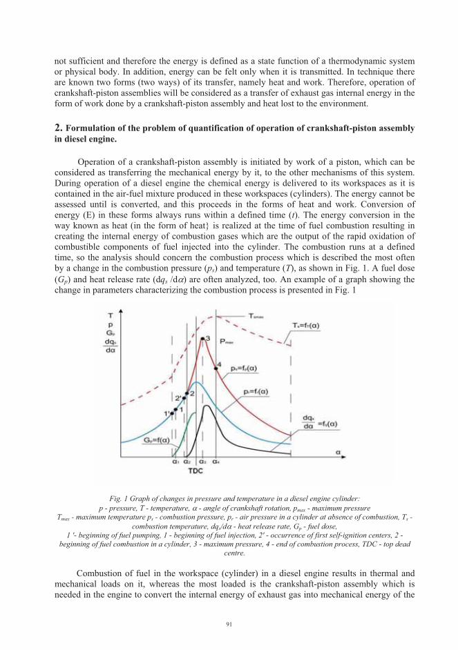
not sufficient and therefore the energy is defined as a state function of a thermodynamic system or physical body. In addition, energy can be felt only when it is transmitted. In technique there are known two forms (two ways) of its transfer, namely heat and work. Therefore, operation of crankshaft-piston assemblies will be considered as a transfer of exhaust gas internal energy in the form of work done by a crankshaft-piston assembly and heat lost to the environment.
2. Formulation of the problem of quantification of operation of crankshaft-piston assembly in diesel engine.
Operation of a crankshaft-piston assembly is initiated by work of a piston, which can be considered as transferring the mechanical energy by it, to the other mechanisms of this system. During operation of a diesel engine the chemical energy is delivered to its workspaces as it is contained in the air-fuel mixture produced in these workspaces (cylinders). The energy cannot be assessed until is converted, and this proceeds in the forms of heat and work. Conversion of energy (E) in these forms always runs within a defined time (t). The energy conversion in the way known as heat (in the form of heat} is realized at the time of fuel combustion resulting in creating the internal energy of combustion gases which are the output of the rapid oxidation of combustible components of fuel injected into the cylinder. The combustion runs at a defined time, so the analysis should concern the combustion process which is described the most often by a change in the combustion pressure (ps) and temperature (T), as shown in Fig. 1. A fuel dose (Gp) and heat release rate (dqs /d�) are often analyzed, too. An example of a graph showing the change in parameters characterizing the combustion process is presented in Fig. 1
Fig. 1 Graph of changes in pressure and temperature in a diesel engine cylinder: p - pressure, T - temperature, � - angle of crankshaft rotation, pmax - maximum pressure
Tmax - maximum temperature ps - combustion pressure, pr - air pressure in a cylinder at absence of combustion, Ts - combustion temperature, dqs/d� - heat release rate, Gp - fuel dose,
1 '- beginning of fuel pumping, 1 - beginning of fuel injection, 2' - occurrence of first self-ignition centers, 2 - beginning of fuel combustion in a cylinder, 3 - maximum pressure, 4 - end of combustion process, TDC - top dead
centre.
Combustion of fuel in the workspace (cylinder) in a diesel engine results in thermal and mechanical loads on it, whereas the most loaded is the crankshaft-piston assembly which is needed in the engine to convert the internal energy of exhaust gas into mechanical energy of the
91

system. This form of energy conversion, as it is known, is called the work. This conversion is accompanied by thermal and mechanical loads on the crankshaft-piston assembly. The mechanical load is a result of the forces and torques acting on the system. An example of a graph of forces acting on the crank system in a trunk engine during fuel combustion in a cylinder is shown in Fig. 2
Fig. 2. Diagram of forces acting on an arbitrary crankshaft-piston assembly in a trunk engine: TDC - top dead centre of piston, BDC - bottom dead centre of piston,
x - piston displacement depending on the angle of crankshaft position (�), Sk - piston stroke, p - pressure acting on piston crown, c - piston speed, N - normal (lateral) force, K - connecting rod force, S - tangential
component of the force K, R - radial component of the force K, P - piston force, l - connecting rod length, � -crankshaft angular velocity, r - crank radius, ? - connecting rod angle, � - crank angle, Tμ - friction force, Qd -supplied heat, Qr - dissipated heat, transferred through workspace walls, L - work done by a crankshaft-piston
assembly, Ś - centre of mass of a connecting rod, a - distance from the mass centre of connecting rod to the centre ofconnecting rod big end (centre of crankpin) in engine crankshaft
It should be kept in mind that all the forces enclosed in the diagram of the forces acting on an arbitrary crankshaft-piston assembly in internal combustion engines (Fig. 2) are random quantities, since combustion is a stochastic process. One of its various realizations is shown in Fig. 1 Similarly, heat loads on pistons and bearings are of a random nature. Despite of this, they may sometimes be considered as deterministic quantities [6, 10].
The net force (P), which is the algebraic sum of the gas force and fictitious force (Fig. 2) acts along the axis of the cylinder.
The force acting perpendicular to the axis of the cylinder (PN) causes piston pressure onto the surface (finishing) of the cylinder sleeve (in case of a trunk engine) and in consequence - friction between the piston and the sleeve, as well as wear of the tribological system.
Qd
aŚ
x
rS
K
K
L
p
R
nagar
SkN
cTμ
P
lβ
α
TDC
BDC
Qr
�
92

The force acting along the axis of the connecting rod (K) is transferred by the connecting rod to the crankpin. Its radial component (R) is carried by the crankpin and crank webs to the crank journal. Thus, it loads the crankpin and crank journal. This force is variable as for its value and action direction. It is considered to be positive while clutching the crank webs. The tangential force (S) not only loads the crank and main bearings, but also causes a momentary torque Mo, whose variability is connected with variability of the tangential force, depending on the angle of rotation of the crankshaft (�) . The forces R and S are defined by the formulas [10]:
?PtgN � ,?cos
PK � ,??�
cos)sin( �
� PS , and )cos(
)cos(?
?� �� PR (1)
From the formula (1) follows that the forces N (lateral, normal), R (radial) and S (tangential force) undergo a change depending on angular position of the crankshaft (�). Theforces change during operation of the crankshaft-piston assembly in a combustion engine, of which the task is to convert (transform) the internal energy of the exhaust gas into mechanical energy. Considering in general the energy conversion at time t (at assumption that the mass of substrates is equal to the mass of exhaust gas), in accordance with the first law of thermodynamics, the following equation can be written down:
U(t) = L(t) + Q(t) (2) where:
U - internal energy of exhaust gas, L - work, Q - heat loss to the environment
Thus, this formula is valid when assuming that during a power stroke the thermodynamic system being the engine's workspace is closed.
The mentioned internal energy of exhaust gas is a sum of the energy of intermolecular and intramolecular interactions and the energy of thermal motion of molecules [11].
When the crankshaft-piston assembly works, during power stroke the exhaust gas expands in a cylinder from TDC (top dead centre) and the combustion pressure decreases from pmax (Fig. 1) to BDC (bottom dead center).
This operation is a result of exhaust gas pressure on the piston crown, which causes a piston displacement from TDC to BDC. When the piston is at TDC, its instantaneous velocity c is equal to zero (c = 0), which means that at this point the kinetic energy of the piston is equal to zero Ek = 0. The piston at TDC position will have a potential (position) energy Ep = mgS with reference to BDC, after reaching which it will return to TDC. This piston movement, however, (from BDC to TDC) will be provided by energy coming from outside (from systems performing work at this time, or from mechanisms which accumulated excess mechanical energy before, eg. from the flywheel). For this reason, this movement is not included in the proposed model of operation of the crankshaft-piston assembly in engine.
During piston displacement from TDC to BDC its speed will increase to the maximum (cmax) and along with the speed - the kinetic energy (Ek > 0) which at this speed will be maximum (Ekmax). From this moment the piston speed decreases, and along with the speed - its kinetic energy. In turn, the potential (gravity) energy of the piston along with its movement from TDC to BDC will decrease from the maximum value (Epmax) at TDC to the zero value at the taken reference position which is BDC (Ep = 0).
Considering the operation of a crankshaft-piston assembly, it should be kept in mind that the internal energy (U) of exhaust gas produced in a cylinder, is converted during transformation into mechanical energy (Em) of the piston and other components of this system, where the piston performs at this time the work (L) on the distance from TDC to BDC. Also at this time the energy is partially lost due to friction existing in tribological pairs in the crankshaft-piston assembly, while being dissipated in the form (in the way) of heat (Q).
93

Considering the operation of a crankshaft-piston assembly leading to execution of a power stroke by its piston it should be remembered that the piston connected to the engine crankshaft through a connecting rod moves flat. This results in that the kinetic energy of the crankshaft-piston assembly is as follows:
� �2222
2
21
21
21
21
��
!"#���
))*
+
,,-
.��
!"#��
�
!"#����
�
!"#������
dtdxm
dtdy
dtdx
mdtdIItE ss
kkk?� (3)
where:I – mass moment of inertia of engine crankshaft with flywheel, Ik – moment of inertia of connecting rod, mk – mass of connecting rod,m �mass of piston,xs , ys � vertical and horizontal coordinate of mass centre (Ś) of connecting rod (Fig. 2),x – piston displacement depending on angle of crankshaft position (�)β – heading angle between connecting rod and piston axis.
In the formula (3) the first component represents the energy of engine crankshaft with a flywheel, second - energy of rotational motion of connecting rod, third - energy of its translational motion, and fourth - energy of translational motion of piston. The equation (3) can be written in the simpler form by applying trigonometric relation between quantities shown in Fig. 2:
�?��
�
�??�?�
sincos
sinsinsinsincoscos
������
������
���������
rlxt
lengthrodconnectingofratiolr
aryarx
s
s
(4) where:
ω - angular velocity of engine crankshaft
By applying the trigonometric formulas (4) the equation (3) can be written as:
� �7 8 2
21 �� ��� FIEk (5)
where: the characteristic function of the system with regard to the crank deflection of the
crankshaft F (� ) is defined as follows
� � � � � �??���
?�?��
�?� 2
2222
22
cossincos
coscossinsin �
���))*
+
,,-
.������
�
!!"
#�������
�
!"#�� rmararm
ddIF kk
where: other designations are as in Fig. 2 and in formulas (3) and (4).
As a piston starts moving from TDC, the kinetic energy of a crankshaft-piston assembly has an initial value Ek0 corresponding to the first so-called "dead" position of the crank for � = 0 and is described by the equation:
94

� �7 8 200 0
21 ���� FIEk (6)
where: � � � �220 armIF kk ������ ��
where: designations are as in formula (4).
During piston movement to BDC, this energy will be greater than zero. (Ek > 0). When the piston is at TDC position the potential energy of the crankshaft-piston assembly calculated with reference to BDC, will be equal to the initial kinetic energy, ie Ep = Ek0.
Therefore, taking into account at the same time the mechanical energy (Em) of the crankshaft-piston assembly and the time of its change, the following equation can be written down:
� �: : ���t t
pkmT ttEtEttEtD0 0
d)()(d)()( (7)
where: DT (t) - piston work, Em - mechanical energy, Ek - kinetic energy Ep - potential energy, t - time
During the so-understood operation of a crankshaft-piston assembly at the time of engine power stroke, the kinetic energy (Ek) increases from the value equal to Ek0 to the maximum value (Ek = Emax ), when the piston reaches the maximum speed (cmax), which takes place in a small distance before the position corresponding to the crank rotation by the angle � = 90 ° [10]. Then, this energy decreases to the value Ek0 at BDC where the piston speed is also zero (c = 0). In turn,the potential energy (Ep), is of the greatest value when the piston is at TDC and is being reduced when the piston moves from TDC, until reaches the lowest value at BDC.
When the piston finds at TDC, additionally at this position it is affected by the internal energy of compressed fresh charge and small internal energy of exhaust gas generated just after self-ignition, at the beginning of the so-called period of flash fire. It can be expected that if the rotational speed n of the crankshaft was then equal to zero, the internal energy of the compressed fresh charge (USŁ) and potential energy of the piston, would not be able to set this system in motion. They would not be able because then their energy would be insufficient to overcome the motion resistance of the system. Motion of the crankshaft-piston assembly is possible only when the conversion of chemical energy of fuel (Echpl), into internal energy of exhaust gas (U),proceeds in continuous manner. Then, part of this energy will cause the piston motion, giving toit the energy Ek. The rest of energy U is dissipated according to the equation (2).
The work of external forces acting on the crankshaft-piston assembly, corresponding to an increment in its kinetic energy, is defined by the equation:
� � � � � � � � ����
����
������
��������� : rRrrPdrRSL AA22
0
sinarcsin2
cos1 (8)
where: S - tangential force (Fig. 2) acting on the crank web of engine crankshaft, RA - utility resistance (power receiver) in engine
The equation (8) shows that operation of a crankshaft-piston assembly is a function of crankshaft rotation angle � and causes a change in its kinetic energy.
The relationship between energy and work for the flat motion [11] being performed by thementioned system, can be written as:
95

� �7 8 � � 00
2
21
kA EdrRSFI ������� :�
��� (9)
In the formula (9) designations have the same interpretation as in the previous formulas.
In practice, the precise equation expressing the relationship between the kinetic energy and work (9) is replaced by an approximate one:
� � � � � � � �7 8 � ��������
GFFdrRSI śrA ������������ : 021
21 2
0
20
2 (10)
where: G(�) – characteristic function of the system.The angular velocity for engine crankshaft is derived from the equation (9), obtaining the
following formula: � � � �
� �����
FILE
dtd k
����
��22 0 (11)
In the formula (11) designations have the same interpretation as in the previous formulas.
The angular velocity of engine crankshaft reaches the values �max or �min for the values of the crankshaft rotation angle �,, which correspond to maximum and minimum of the function G(�). Values Gmax and Gmin are calculated on the basis of indicator diagram by taking into account the tangential force S (Fig. 2) which is a function of the angle � and afterwards the motion resistance force (RA) of the engine crankshaft-piston assembly (utility resistance) is determined from the condition:
� �: �����
�0
0drRS A (12)
The motion resistance force can also be derived by differentiating the equation (9) as follows:
� �7 8 � � � �
� �7 8 � �@AB
%&'
��������
���������
22
2
22
2
211
021
�����
�����
ddF
dtdFI
rSR
hence
rSRd
dFdtdFI
A
A
(13)
Therefore, taking into account the dynamics of the crankshaft-piston assembly [6, 10], its operation during the power stroke can be (in general terms) defined as follows:
� � � � � � 222
2sinarcsincos1 tRrtrrPtD A �����)
*
+,-
.�
������� �
���� (14)
where: designations are as in the previous formulas.
From the formula (14) follows that at the operating time of piston performing a work, the kinetic energy obtained from the internal energy of exhaust gas is consumed. Therefore, when the piston is under operation the energy is converted into work, which consists in changing a part
96

of the internal energy of exhaust gas into kinetic energy of the piston. Additionally, the potential energy which the piston owns being at TDC, takes also part in the conversion.
The time (t) of piston operation can be determined on the basis of the following reasoning. During piston motion from TDC to BDC, which enables execution of work by a piston force Pmade above the piston while travelling the distance S (piston stroke), the piston moves atsubsequent moments by a defined value x dependent on the angle (�)) of the crankshaft position (Fig. 2) [10].
Integrating the equation (11) gives the formula for the motion, from which the time of piston operation is calculated as follows:
� �� � � �7 8 �
���
dLE
FItk
���
�� :
0 02 (15)
where: designations are as in the previous formulas.
By applying the given formulas, the following difficulties arise: although the forms of the functions F(�) and L(�} are known we do not know the values Ek0 because unknown is the angular velocity �0 corresponding to the initial energy Ek0. These difficulties are solved by adopting the average value of angular velocity �0 and applying the equations from which the velocity �0 is derived:
� �� �7 8 � �
T
dLFI
FI
śr
śr
��
���
��� �
20
2 2
020
�
����
�� :
(16)
where: T – period of one rotation of engine crankshaft.
The presented proposal of analysis and valuation of operation of a crankshaft-piston assembly during piston motion from TDC to BDC at the time of power stroke, can be applied when the assumption can be accepted that the combustion process is not a stochastic process. If this assumption cannot be accepted, the statistical methods need to be applied.
The internal energy provides motion of the piston from TDC to BDC, during which isconverted in the form of work into mechanical energy of a crankshaft-piston assembly. However, only a part of this energy is converted to mechanical energy of CPA (according to the second law of thermodynamics), the rest is dissipated to the environment as energy being lost due to friction in its tribological pairs and the energy loss because of existing differences in temperature between exhaust gas and CPA components and the ambient temperature.
From the considerations follows that only a part of the internal energy of exhaust gas makes motion of PCS' components and the rest undergo dissipation as different types of energy.
Operation of crankshaft-piston assemblies over time will require more and more internal energy of exhaust gas, because the energy losses will increase due to:
• increase in exhaust gas flow between the piston and the cylinder liner into the under piston space because of wear of rings or their immobilization in the grooves as a result of occurrence of exhaust carbon,
• increase in friction between the piston and the sleeve and bearings of the crankshaft and the piston pin bearing, if the piston is connected to the connecting rod through a pin,
• scuffing of the piston in the cylinder liner.This results from wear of the mentioned tribological pairs in engine crankshaft-piston assemblies and from aging lubricating oil.
97
The technical diagnostics is needed to be applied in order to obtain information on the process of the exhaust gas flow as well as friction and wear in specific tribological pairs of crankshaft-piston assemblies in a combustion engine.
3. Remarks and conclusions
The proposed interpretation for operation of crankshaft-piston assemblies (CPA) in engine is the first such attempt, presented in general terms. However, it requires more precise defining,which will not be easy because of the need for detailed identification of all energy types which undergo conversion at the time of CPA operation.
The proposed evaluation method for operation of a crankshaft-piston assembly leading to execution a power stroke by its piston, reflects the observation that the piston connected to the engine crankshaft via a connecting rod performs a flat motion.
Certainly, the provided considerations on CPA operation have cognitive advantages, but at this moment it is difficult to determine how much important to science. In turn, the utilitarian values are difficult to be assessed because of problems with implementation of relevant empirical research.
CPA operation requires defining a change in not only energy but also time of its conversion. Both the amount of converted energy which manifests itself in the ways (forms) of its conversion, as well as the operating time of CPA operation, during which the energy conversion proceeds, depend on the technical state of its components, particularly a piston which is the most loaded mechanism. Thus, quantification of the operation requires application of an adequate measuring technique.
REFERENCES
1. Girtler J.: Work of a compression-ignition engine as the index of its reliability and safety. II International Scientifically-Technical Conference EXPLO-DIESEL & GAS TURBINE”01. Conference Proceedings. Gdansk-Miedzyzdroje-Copenhagen, 2001, pp.79-86.
2. Girtler J.: Possibility of valuation of operation of marine diesel engines. Journal of POLISH CIMAC, Vol 4, No 1, 2009.
3. Girtler J.: Energy-based aspect of operation of diesel engine. COMBUSTION ENGINES No 2/2009 (137).
4. Gribbin J.: In Search of Schrödinger’s Cat Quantum Physics Reality. Wyd. polskie: W poszukiwaniu kota Schrödingera. Zysk i S-ka Wydawnictwo s.c. Poznań 1 997.
5. Helwitt P.G.: Fizyka wokół nas. PWN, Warszawa 2001.6. Piotrowski I., Witkowski K.: Okrętowe silniki spalinowe. Wyd. TRADEMAR, Gdynia 1996.7. Rosłanowski J.: Identification of ships propulsion engine operation by means of dimensional
analysis. Journal of POLISH CIMAC, Vol. 4, No 1, 2009. 8. Rudnicki J.: Loads of ship main diesel engine in the aspect of practical assessment of its
operation. Journal of POLISH CIMACE, Vol. 3, No 1, 2008.9. Rudnicki J.: On making into account value of operational applied to ship main propulsion
engine as an example. Journal of POLISH CIMAC, Vol. 4, No 1, 2009. 10. Wajand J.A., Wajand Jan T.: Tłokowe silniki spalinowe średnio- i szybkoobrotowe. WNT,
Warszawa 2000.11. Wittbrodt E., Sawiak: Mechanika ogólna. Teoria i zadania. Wyd. Politechnika Gdańska,
Gdańsk 2005.12. Encyklopedia fizyki współczesnej. Praca zbiorowa. Redakcja Nauk Matematyczno-
Fizycznych i Techniki Zespołu Encyklopedii i Słowników PWN. PWN, Warszawa 1983.13. Leksykon naukowo-techniczny z suplementem. Praca zbiorowa. Zespół redaktorów Działu
Słownictwa Technicznego WNT. WNT, Warszawa 1989.
98

PERFORMANCE AND EMISSION CHARACTERISTICS OF THE DIESEL ENGINE OPERATING ON THREE-COMPONENT FUEL
Gvidonas Labeckas, Stasys Slavinskas
Lithuanian University of Agriculture, Students street, 11, LT-53361 Kaunas-Academy, E-mail: [email protected]; [email protected];
Abstract
The article deals with bench testing results of a DI (60 kW) diesel engine D-243 operating on reference (DF) arctic class 2 diesel fuel (80vol%), anhydrous (200 proof) ethanol (15vol%) and rapeseed methyl ester (5vol%) blend B15E5. The purpose of the research is to investigate the effect of simultaneous ethanol and RME addition in the diesel fuel on brake specific fuel consumption (bsfc), the brake thermal efficiency (ηe) and noxious emissions, including NO, NO2, NOx, CO, CO2, HC and smoke opacity of the exhausts. The bsfc of the diesel engine operating on three-component fuel B15E5 under maximum load of bmep = 0.75, 0.76 and 0.68 MPa is higher by 10.3%, 10.7% and 9.6% because of both net heating value lower by 6.18% and brake thermal efficiency lower by 3.4%, 3.7% and 2.8% relative to that of reference diesel at 1400, 1800 and 2200 min-1 speeds. The maximum NOx emission produced from oxygenated blend B15E5 was reduced by 13.4%, 18.0% and 12.5% and smoke opacity diminished by 13.2%, 1.5% and 2.7% under considered loading conditions relative to that of a neat diesel fuel. The CO amounts produced from three-component fuel B15E5 were lowered by 6.0% for low 1400 min-1 speed only and they increased by 20.1% and 28.2% for higher 1800 and 2200 min-1 speeds and the HC emissions were also higher by 35.1%, 25.5% and 34.9% throughout a whole speed rage comparing with respective values measured from neat diesel fuel.
Key words: diesel engine, diesel fuel, anhydrous ethanol, rapeseed oil methyl ester, brake specific fuel mass consumption, NOx, CO, HC emissions, smoke opacity
1. Introduction
Both high prices of mineral fuels and society’s concern about global warming encourage researchers to intensify investigations on alternative and renewable energy sources, which could diminish the CO2 emission in a global cycle. As potential mineral fuel extender bioethanol is indigenous and locally available, environment friendly and renewable, sustainable and reliable, safe to store and easy to handle, non-polluting and sulphur-free material, and is one of the cleaner-burning alternatives to mineral fuels. In order to solve technical problems, there several methods can be adapted to employ a certain amount of ethanol for diesel engine fuelling, which are known as alcohol fumigation [1], application of a dual injection systems [2], preparation of the alcohol-diesel fuel micro-emulsions [3] and using of the alcohol-diesel fuel blends [1,4-6].
Investigations conducted on a single cylinder DI, variable compression ratio diesel engine [1]confirmed that biofuel blends prepared by mixing of anhydrous (200 proof) ethanol and diesel fuel would also be acceptable for the diesel engine fuelling when applied in proper up to 15% proportions. Advantages and disadvantages of ethanol additives used for rapeseed oil treatment and diesel engine fuelling have been elucidated in reports [7,8]. The molecular weight of ethanol is lower 3.91 times, its density at temperature of 20 oC is lower by 4.9% and kinematic viscosity at temperature of 40 oC is also lower 1.47 times relative to that of the diesel fuel, which together with
99

a low CFPP at the temperature below of –38 oC may elevate biofuel flow in the fuelling system and improve starting of the engine under winter conditions.
The miscibility of anhydrous ethanol with the diesel fuel is excellent and it makes clear one phase mixture however during a long-term application of ethanol-diesel mixtures the lubrication problems of the injection pump’s plunger-barrel unit may emerge at higher than 15vol% blending ratios. To improve lubrication properties of the blend and increase the content of biofuel in the mixture RME from 5vol% to 10vol% as co-solvent can be recommended for ethanol-diesel blends [9,10]. The addition of RME as a stabilizer of ethanol-diesel mixture, suggests an extra advantage because this method allows avoid phase separation between the pure diesel fuel and the ethanol fraction during long term storage.
The purpose of the research was to study the effect of anhydrous (200 proof) ethanol and rapeseed oil methyl ester (RME) addition to arctic class 2 diesel fuel on biofuel properties and conduct comparative bench tests to examine changes in the brake specific fuel consumption (bsfc), the brake thermal efficiency (ηe) and the emission composition, including nitrogen oxides NO, NO2, NOx, carbon monoxide CO and dioxide CO2, total unburned hydrocarbons HC, residual oxygen O2 content and smoke opacity of the exhausts when running the engine alternately on a neat diesel fuel and three-component blend B15E5 containing 80vol% diesel fuel, 15vol% ethanol and 5vol% RME over a wide range of loads and speeds.
2. Objects, apparatus and methodology of the research
Tests have been conducted on four stroke, four cylinder, DI (60 kW) diesel engine D-243 with a splash volume Vl = 4.75 dm3, bore 110 mm, stroke 125 mm and compression ratio ε = 16:1. The fuel was delivered by an in line fuel injection pump thorough five holes injector nozzles with the fuel delivery starting at 25o before TDC.
The three-component blend was prepared by pouring diesel fuel (80vol%), anhydrous (99.81 purity) ethanol (15vol%) and RME (5vol%) into container and mixing them to keep the blend prepared in homogeneous conditions. Three-component biofuel B15E5 distinguishes itself as having the fuel bond oxygen mass content 6.1%, stoichometric air-to-fuel equivalence ratio 13.55 kg/kg and net heating value 39.92 MJ/kg.
Load characteristics were taken at speeds of 1400, 1800 and 2200 min-1 when operating alternately on neat diesel fuel (arctic class 2) and ethanol-diesel-biodiesel blend B15E5. The torque of the engine was increased from close to zero point up to its maximum values those correspond standard bmep = 0.75, 0.76 and 0.68 MPa changing behaviour at respective speeds.
The torque of the engine was measured with 110 kW AC stand dynamometer with a definition rate of ±0.5 Nm and the rotation speed was determined with the universal stand tachometer TSFU-1 that guarantees the accuracy of ±0.2%. The fuel mass consumption was measured by weighting it on the scale SK-1000 with accurateness of ±0.05 g and the volumetric air consumption was determined with the rotor type gas counter RG-400-1-1.5. The time spent for consumption of 2 m3
of air and 100 g of fuel has been measured with the second-meter with a definition rate of ±0.01 s. The amounts of carbon monoxide CO (ppm), dioxide CO2 (vol%), nitric oxide NO (ppm) and
nitrogen dioxide NO2 (ppm), unburned hydrocarbons HC (ppm vol%) and the residual oxygen O2(vol%) content in the exhaust manifold were measured with a flue gas analyser Testo 350 XL. Smoke density D (%) of the exhausts was measured with a Bosch RTT 100/RTT 110 opacity-meter, the readings of which are provided as Hartridge units in scale I - 100% with the accuracy of ±0.1%.
3. Results and discussions
The addition of 15vol% of ethanol and 5vol% of RME into diesel fuel does not change greatly
100

density and kinematic viscosity of biofuel blend relative to respective values of a neat diesel fuel because the lower density (790.0 kg/m3) at temperature of 20 oC and critically reduced viscosity (1.40 mm2/s) at temperature of 40 oC of ethanol were compensated with 1.12 times higher density (884.7 kg/m3) and 3.42 times bigger viscosity (4.79 mm2/s) of RME portion premixed. Because of simultaneous addition of improving additives having different chemical and physical properties the injection and atomisation characteristics of three-component fuel B15E5 should not vary much from those of a neat diesel fuel.
Tab.1. Testing conditions of the diesel engine operating on arctic class 2 diesel fuel and ethanol-diesel-biodiesel blendB15E5
Rotation speed, min-1
Brake mean effective pressures, MPa for both cases DF and B15E5 Air-to-fuel equivalence ratio λheavy medium light DF B15E5
1400 0,75 0.47 0.14 1,45 2.39 5.30 1,42 2.31 5.061800 0,76 0.44 0.15 1,42 2.47 5.21 1,37 2.38 5.732200 0,68 0.41 0.07 1,49 2.31 6.14 1,47 2.32 5.93
light
medium
heavy
1400 DF1800 DF
2200 DF1400
B15E5
1800B15E5
2200B15E5
100
200
300
400
500
600
700
bsfc
, g/(k
Wh)
load
Fig. 1. The brake specific fuel consumption (bsfc) for neat diesel fuel and three-component fuel B15E5 as a function of engine load and speed
As is shown in Table 1, comparative analysis of the engine performance parameters and its emission changes when operating alternately on neat diesel fuel and ethanol-diesel-biodiesel blend B15E5 was conducted for light, medium and heavy loading conditions, i.e. for both cases under the same brake mean effective pressures developed at respective 1400, 1800 and 2200 min-1
speeds. The biggest values of bmep = 0.75, 0.76 and 0.68 MPa correspond to standard torque changing behaviour of the engine versus crankshaft’s rotation speed of 1400, 1800 and 2200 min-1.Such approach suggests a little bit lower air-to-fuel equivalence ratios for biodiesel that should be taken into account when considering engine performance and its emission composition changes.
As it follows from the analysis of columns in Fig. 1, the biggest 14.9% and 12.0% increase in the brake specific fuel consumption (bsfc) relative to that of a mineral diesel (356.7 g/kWh and 598.0 g/kWh) takes place when running of the easy loaded engine on blend B15E5 at critical speeds of 1400 and 2200 min-1. In the case of using in-line fuel injection pump the combustible mixture prepared at extremely light load is more heterogeneous that together with a lower cetane number of ethanol-diesel-biodiesel blend may aggravate the autoignition leading to incomplete combustion of small fuel portions injected at low and high speeds. Nevertheless, performance
101

efficiency of the easy loaded (0.15 MPa) biodiesel improves at speed of 1800 min-1 corresponding maximum torque mode where the bsfc diminishes to 348.5 g/kWh and difference in specific fuel consumptions between considered cases reduces to 5.3%.
After load of the engine increases to medium and heavy values the bsfc of three-component fuel remains higher by 8.4%, 10.8, 10.5% and 10.3%, 10.7%, 9.6% comparing with that of a neatdiesel fuel at speeds of 1400, 1800 and 2200 min-1. The bigger biofuel mass consumption spent for the same amount of energy produced can be attributed primarily to lower, on average by 6.18%, net heating value (39.52MJ/kg) of three-component fuel B15E5 comparing with that of the diesel fuel (42.55 MJ/kg). However difference in the heating value of the tested fuels is probably not the main reason that leads to the higher three-component fuel consumption in grams per unit of energy developed.
After substitution of the diesel fuel (0.24) with blend B15E5 the biggest 7.3% decrease in brake thermal efficiency was suffered when operating at light 0.14 MPa load and low 1400 min-1
speed. Whereat the performance mode of biodiesel was changed to medium and heavy loads the ηeincreased to 0.32-0.34 sustaining at lower by 1.6%, 3.8%, 3.6% and 3.4%, 3.7%, 2.8% levels relative to values determined for reference diesel at 1400, 1800 and 2200 min-1 speeds. The lower thermal efficiency of biodiesel can be attributed to changes occurring in the combustion process [1]. Extremely low cetane number (8) of ethanol, its low calorific value (26.82 MJ/kg) along with a high volatility and significant cooling effect of the fuel sprays caused by 3.5 times bigger latent heat for evaporation (910 kJ/kg) relative to that of the diesel fuel and tendency to absorb ambient water may aggravate the autoignition of biofuel portions injected resulting into retarded start of combustion, relocating the maximum cylinder gas pressure and temperature points towards the expansion stroke and increasing incomplete diffusion burning of fuel reach portions [12]. A twice as much higher autoignition temperature (420 oC) of ethanol relative to that of diesel fuel (230 oC) aggravates autoignition and provokes misfiring cycles at easy loads and sharp knocking under heavy loads for bigger than 15vol% ethanol additions [9].
light
medium
heavy
1400 DF1800 DF
2200 DF1400
B15E5
1800B15E5
2200B15E5
100
300
500
700
900
1100
1300
1500
1700
NO
x, p
pm
load
Fig. 2. Total nitrogen oxides NOx emissions produced from diesel fuel and three-component fuel B15E5 as a function of engine load and speed
As it follows from data given in Table 1, to develop the same torque and effective power as that of reference diesel a fully loaded engine run on less (by 6.18%) calorific three-component fuel B15E5 is imposed to operate with a bigger fuel mass portion delivered per cycle, i.e. under air-to-fuel equivalence ratios on average lower by 2.1%, 3.5% and 1.3% at respective speeds. Engine performance under marginal oxygen deficiency can be one of a main reason why the brake thermal efficiency of biodiesel was lower and the bsfc of oxygenated (6.1% oxygen) fuel was accordingly
102

higher than that of reference diesel. Incomplete combustion of biofuel blend tested results into corresponding changes in NOx (Fig. 2), CO (Fig. 3) and HC (Fig. 4) emissions behaviour.
The amounts of NOx emissions depend on performance conditions of the engine, the feedstock oil used for engine fuelling and iodine number, the composition and chemical structure of the fatty acids as well as on variations in actual fuel injection timing advance and autoignition delay caused by changes in physical properties, such as the effect of bulk modulus, viscosity and density of the biofuel [11,12]. A key role in the NOx production plays also oxygen mass (weight) content accumulated in the biofuel, its composition and chemical structure, including presence of double bonds, as well as performance efficiency related maximum cylinder gas temperature [8,11,13]. Test results with a Case model 188D four cylinder, DI diesel engine confirm that up to 60% of replacement of diesel fuel by ethanol can be achieved however engine misfiring appears because of extreme autoignition delay and severe knocking occurs under some testing conditions [2].
Fig. 3. Emissions of carbon monoxide CO produced from diesel fuel and three-component fuel B15E5 as a function of engine load and speed
Analysis of columns in Fig. 2 indicates, that maximum NOx emissions produced by the engine operating on three-component fuel B15E5 are lower by 13.4% (1394 ppm), 18.0% (1416 ppm) and 12.5% (1129 ppm) throughout the whole speed range comparing with those values generated from diesel fuel. The intermediate NOx emission values determined for biodiesel operating under light and medium loads, as it is shown by headmost columns, are also lower by 39.6%, 14.4%, 27.1% and 32.5%, 18.7%, 21.2% at respective 1400, 1800 and 2200 min-1 speed.
In spite of a higher fuel bond oxygen mass content (6.1%), worse performance efficiency of biodiesel and lower maximum cylinder gas temperature does not create conditions necessary for production of NOx [13]. Experiments conducted with a turbocharged and intercooled 7.3 l diesel engine T 444E HT confirmed that maximum cylinder gas pressures and temperatures decreased slightly with increasing the proportion of ethanol, therefore benefits in reduced NOx emissions were also observed, ethanol-diesel blend E10 decreased NOx emissions by close to 3% [4].
0
200
400
600
800
1000
1200
1400 1800 2200
n, rpm
CO
, ppm
DF B15E5
bmep = 0,14 MPa
bmep = 0,15 Mpa
bmep = 0,07 Mpa
0
100
200
300
400
500
1400 1800 2200
n, rpm
CO
, ppm bmep = 0,47 MPa bmep = 0,44 MPa
bmep = 0,41 MPa
0
200
400
600
800
1000
1200
1400
1400 1800 2200
n, rpm
CO
, ppm
bmep = 0,75 MPa
bmep = 0,76 MPa bmep = 0,68 MPa
103

The carbon monoxide CO emissions depend on load, hence quantity of fuel delivered per cycle and air-to-fuel equivalence ratio, engine speed, i.e. cylinder air swirl turbulence intensity, and biofuel conserved oxygen mass content. When operating on three-component fuel B15E5 at light and under medium loads CO emissions emanating from biodiesel are bigger by 99.7% (759 ppm), 6.4% (598 ppm), 35.3% (1054 ppm) and 15.7% (236 ppm), 22.2% (242 ppm), 45.5% (384 ppm) relative to those determined for reference fuel at 1400, 1800 and 2200 min-1 speeds (Fig. 3).
In the case of running a fully loaded engine, the CO emissions produced from blend B15E5 are lower by 6.0% (992 ppm) only at a low 1400 min-1 speed and they increase against those measured from reference diesel by 20.1% (1248 ppm) and 28.2% (913 ppm) for higher speeds. Diminished CO emissions at low revolutions can be attributed to a lower C/H ratio of blend B15E5 (6.45) comparing with that of the diesel fuel (6.90) whereas significant CO increase at higher speeds of 1800 and 2200 min-1 may take place due to worse ethanol operating properties and such result matches well with a lower NOx emission (Fig. 2) emerging from biodiesel.
Fig. 4. Emissions of total unburned hydrocarbons HC produced from diesel fuel and three-component fuel B15E5 as a function of engine load and speed
Emissions of HC generated from fuel B15E5 are higher throughout a whole load and speed range (Fig. 4). The biggest 65.5% (960 ppm) HC emission increase occurs at light load and low speed because of diminished fuel injection pressure, cylinder air swirl turbulence intensity, gas pressure and temperature. As speed of the easy loaded biodiesel increases to 1800 and 2200 min-1
HC emissions scale up to 970 and 1070 ppm, however their increments regarding baseline values diminish to 16.9% and 37.2%. When running at medium load the HC emission generated from blend B15E5 sustains actually at the same 800 ppm level for a whole speed range, i.e. is by 48.1%, 23.1%, 27.0% higher respective to its baseline values, and increases again to 1270 ppm (35.1%), 1280 ppm (25.5%), 1160 ppm (34.9%) for heavy loads. The test results of a single cylinder Cummins 4 type engine indicate that with increasing ethanol percentage in the blended diesel fuel reduction in NOx varied from zero to 4-5%. Both decreases and increases in CO emissions
0
200
400
600
800
1000
1200
1400 1800 2200n, rpm
HC
, ppm
DF B15E5
bmep = 0,14 MPa bmep = 0,15 Mpabmep = 0,07 Mpa
0
200
400
600
800
1000
1400 1800 2200
n, rpm
HC
, ppm
bmep = 0,47 MPa bmep = 0,44 MPa bmep = 0,41 MPa
0
200
400
600
800
1000
1200
1400
1400 1800 2200
n, rpm
HC
, ppm
bmep = 0,75 MPa bmep = 0,76 MPabmep = 0,68 MPa
104

occurred, while THC increased substantially, but both were still well below the regulated emissions limit [5].
Because of incomplete burning at light load and low speed, the smoke opacity appearing from three-component fuel B15E5 is vaporous and compiles only 1.5%, however it increases to 5.1% and 5.5% becoming by 70.0% and 14.6% bigger, for higher 1800 and 2200 min-1 speeds (Fig. 5). Vaporous smoke emerging from the easy loaded biodiesel matches well with a bigger specific fuel mass consumption (Fig. 1), higher CO (Fig. 3) and HC (Fig. 4) emissions and reasonably lower emission of NOx (Fig. 2). In the case of running partially loaded biodiesel smoke opacity does not change greatly with speed sustaining actually at the same 20.1-20.5% level, however it is by 32.0% (1400 min-1) to 99.0% (1800 min-1) bigger than that produced from neat diesel fuel.
When operating of the fully loaded engine on fuel B15E5 smoke opacity was reduced by 13.2%, 1.5% and 2.7% comparing with its baseline 61.3%, 66.0% and 69.6% values generated from reference diesel at 1400, 1800 and 2200 min-1 speeds. Experiments conducted in a steel combustion chamber with 5vol%, 10 vol% and 20vol% ethanol-diesel blends showed that blending diesel fuel with additives having considerably higher H/C ratios improves the combustion process, reducing pollutants and soot mass concentration in the exhausts [3]. However, when using biofuel B15E5 the fuel bond oxygen may come into effect with a little help and, rather, to late to improve performance efficiency of the engine reducing CO, HC and other related emissions [14].
light
medium
heavy
1400DF
1800DF
2200DF
1400B15E5
1800B15E5
2200B15E5
0
20
40
60
80
100
Exh
aust
opa
city
, %
load
Fig.5. Smoke opacity of the exhausts produced from neat diesel fuel and three-component fuel B15E5 as a function of engine load and speed
In the case of running a fully loaded engine on biofuel B15E5 residual oxygen O2 content in the exhausts was lower, on average, by 5.0% (7.17vol%), 7.4% (6.10vol%) and 4.3% (7.16vol%) and carbon dioxide CO2 emission was higher by 2.8% (10.21vol%), 3.4% (10.99vol%) and 2.4% (10.22vol%) relative to that measured from neat diesel fuel at 1400, 1800 and 2200 min-1 speeds.
Conclusions 1. Test results indicate that when operating of a fully loaded engine on three-component fuel
B15E5 the brake specific fuel mass consumption is bigger by 10.3%, 10.7% and 9.6% comparing with that 237.2, 239.5 and 244.7 g/kWh of a neat diesel fuel. Substitution of the diesel fuel with oxygenated (6.1% oxygen) fuel B15E5 results into the brake thermal efficiency of the fully loaded engine lower by 3.4%, 3.7%, 2.8% relative to values determined for a neat diesel fuel at respective 1400, 1800 and 2200 min-1 speed.
105
2. Maximum emissions of NOx produced from three-component fuel B15E5 were diminished by 13.4%, 18.0% and 12.5% throughout a whole speed 1400, 1800 and 2200 min-1 range relative to 1609 ppm, 1539 ppm and 1291 ppm generated from neat diesel fuel that can be attributed reasonably to worse performance efficiency of biodiesel.
3. The carbon monoxide, CO, emissions from biodiesel are bigger by 99.7% for light 0.14 MPa load and 1400 min-1 speed relative to reference 380 ppm value, however difference in the CO amounts exhausted descents by 6.0% (992 ppm) below reference level for the maximum load of 0.75 MPa and low speed of 1400 min-1 increasing again by 20.1% (1248 ppm) and 28.2% (913 ppm) for higher 1800 and 2200 min-1 speeds.
4. The biggest 65.5% (960 ppm) increase in emission of the HC regarding reference diesel fuel occurs at a light 0.14 MPa load and reduced 1400 min-1 speed. When operating under full load, the three-component fuel B15E5 suggests HC emission bigger by 35.1% (1270 ppm), 25.5% (1280 ppm) and 34.9% (1160 ppm) at corresponding 1400, 1800 and 2200 min-1 speed.
5. Smoke opacity emerging from a fully loaded engine operating on oxygenated fuel B15E5 is lower by 13.2%, 1.5% and 2.7% relative to respective 61.3%, 66.0% and 69.6% values measured from neat diesel fuel at speeds of 1400, 1800 and 2200 min-1. Residual oxygen O2content in the exhausts is lower by 5.0%, 7.4%, 4.3% and carbon dioxide CO2 emissions are bigger by 2.8%, 3.4%, 2.4% when operating under full throttle on three-component fuel B15E5 relative to that measured from neat diesel fuel at respective speeds.
References
[1] Abu-Qudais, M., Haddad, O., Qudaisat, M. The effect of alcohol fumigation on diesel engine performance and emissions. Energy Conversion and Management, 2000, Vol. 41, p. 389-399.
[2] Shropshire, G.J., Goering, C.E. Ethanol injection into a Diesel-engine. Transactions of the ASAE, Vol. 25(3) 1982, p. 570-575.
[3] Asfar, K.R., Hamed, H. Combustion of fuel blends. Energy Conversion and Management, 1998, Vol. 39, Issue 10, p. 1081-1093.
[4] Hansen, A.C., Gratton, M.R., Yuan, W. Diesel engine performance and NOx emissions from oxygenated biofuels and blends with diesel fuel. Transactions of the ASAE, 2006, Vol. 49 (3), p. 589-595.
[5] Hansen A.C., Zhang Q, Lyne P.-W.L. Ethanol-diesel fuel blends – a review. Bioresource Technology, 2005, Vol. 96, p. 277-285.
[6] Jha, S.K., Fernando, S., Columbus, E., Willcutt, H. A comparative study of exhaust emissions using diesel-biodiesel-ethanol blends in new and used compression ignition engines. Paper Number: 066138. An ASABE Meeting Presentation, Portland, Oregon, USA, 9-12 July 2006. p. 12.
[7] Labeckas, G., Slavinskas, S. Comparative performance of direct injection Diesel engine operating on ethanol, petrol and rapeseed oil blends. Energy Conversion and Management, Vol. 50 (2009), Issue 3, p. 792-801.
[8] Labeckas, G., Slavinskas, S. Study of exhaust emissions of direct injection Diesel engine operating on ethanol, petrol and rapeseed oil blends. Energy Conversion and Management, Vol. 50 (2009), Issue 3, p. 802-812.
[9] Xing-cai, L., Jian-guang, Y., Wu-gao, Z., Zhen, H. Effect of cetane number improver on heart release rate and emissions of high speed diesel engine fuelled with ethanol-diesel blend fuel. Fuel, Vol. 83, 2004, p. 2013-2020.
[10] Chen, H., Shuai, S-J., Wang, J-X. Study on combustion characteristics and PM emission of diesel engine using ester-ethanol-diesel blended fuels. Proceedings of the Combustion institute, Vol. 31, 2007, p. 2981-2989.
106

[11] Graboski, M.S., McCormick, R.L. Combustion of Fat and Vegetable Oil Derived Fuels in Diesel Engines. Progress in Energy and Combustion. Scientific. Vol. 24 1998, p. 125-164, Elsevier Science Ltd.
[12] Lotko, W., Lukanin, V.N., Khatchiyan, A.S. Usage of Alternative Fuels in Internal Combustion Engines. –Moscow: MADI, 2000. –311 p. (in Russian).
[13] Heywood, J.B. Internal Combustion Engine Fundamentals. –Co - Singapore for manufacture and export (International edition) 1988. 930 p.
[14] Rakopoulos C.D., Antonopoulos K.A., Rakopoulos D.C., Hountalas D.T., Giakoumis E.G. Comparative performance and emissions study of a direct injection Diesel engine using blends of Diesel fuel with vegetable oils or bio-diesels of various origins. Energy Conversion and Management. 2006, Vol. 47, p. 3272-3287.
The paper was published by financial supporting of West Pomeranian Province
107

108

USING INFORMATION FROM AIS SYSTEM IN THE MODELLING OF EXHAUSTS COMPONENTS FROM MARINE MAIN DIESEL ENGINES
Tomasz Kniaziewicz, Leszek Piaseczny
Polish Naval Academy, Faculty of Mechanical and Electrical Engineering
ul. Śmidowicza 69, 81-103 Gdynia, Poland tel.: +48 58 6262851, 6262665
e-mail: [email protected], [email protected]
Abstract
Society’s growing pro-ecological pressure has made atmosphere pollution by marine diesel engine exhausts one of the main problems of marine environment protection of recent years. In order to determine the share of vessels in atmospheric air pollution and to counteract the harmful effects of toxic compounds in marine engines exhausts, it is necessary to know the emission values of these compounds from particular vessels, which is possible if one knows the vessel movement parameters, concentration values of particular compounds for these parameters and the atmos-pheric conditions in the area they are staying in.
The work presents conditions concerning the modelling of harmful compounds emission of engine exhausts based on the example of ships sailing in the Gulf of Gdańsk region, using infor-mation from AIS system.
Key words: emission, exhausts, toxic compounds, modelling, narine engines, AIS
1. Introduction The problem of air pollution in ports and approaches to ports is important insomuch as ports
are usually located close to or in the area of large cities, and their restricted space is the cause of large concentration of vessels in a small area. Widely conceived operational conditions are not without significance either. Among the latter there can be counted the way of operating the en-gines, frequency and character of steady and transient conditions, and external conditions affecting engine work. Exhausts toxicity is also affected by the kind of fuel and lubricating oil applied
Research conducted currently throughout the world concerning atmosphere pollution caused by emission of toxic compounds from ship engines, conceived both globally [1,2] and regionally [3,4], as also locally, e.g. in areas of large sea ports [5] is based on simplified input data [2,6,7]. The existing data bases of harmful compounds emission from exhausts of ships sailing in various regions of the world [7] cannot be used, however, for the estimation of emission in mezzo- and
109

microscale, e.g. The Baltic Sea or the Gulf of Gdansk, as they lead to considerable underestimation of emission indexes, mainly due to too few details of vessel movement characteristics [8].
The factors determining global emission of substances contained in marine diesel engines ex-hausts have been classified and described in [4].
The process of modelling of toxic compounds (TC) emission in marine engines exhausts is very complex and requires information that can be divided into four basic groups:
� vessel parameters – length, breadth and draft of the vessel, technical condition of the pro-pulsion system, kind of propulsion (including kind and number of engines), kind and number of propulsion screws etc.;
� vessel movement parameters – vessel’s course and speed;� external conditions – wind direction and force, air and water temperature, atmospheric
pressure, air humidity, state of the sea; � number of vessels with consideration of their categories.
Models of emission from inland transports created in Europe, like HBEFA, COPERT, DVG, DRIVE-MODEM attempt to take into account the largest possible number of parameters affecting emission, yet with such a large number of factors and complex description of phenomena determining the emission process, simplifying assumptions cannot be avoided. Besides, due to the difference in both hydrometeorological conditions and the specificity of vessel operation, they cannot be applied for the assessment of emission from ships.
The STEAM model (Ship Traffic Emission Assessment Model) of toxic compounds emission presented in [9] is based on data transmitted by the AIS system and calculations are made on their basis of toxic compounds emission indexes in the exhausts. Yet even in this model no simplifying assumptions have been avoided (for instance, when engine data were unavailable it was assumed that it was a medium-speed engine with self-ignition of rated rotation speed of n=500 rpm, which is likely to cause that the determined emission indexes will not reflect real emission values.
There exists thus the need to apply methods by means of which it will be possible to deter-mine much more precisely the characteristic of vessel movement as also the emission values.
2. General characteristic of AIS system
The AIS (Automatic Identification System) is a radio system that enables automatic exchange of information of vessel identification, essential for vessel traffic safety in relation ship-to-ship, ship- to-plane and ship-to-shore.
According to MSC 74 (69) resolution of the Safety-at-Sea Committee of International Mari-time Organisation [10] of newly-built vessels (of 300 BRT tonnage and larger in international shipping and 500 BRT and larger) were to be equipped systematically starting from 1 June 2002.
According to IMO recommendations, the AIS installed on the vessel should automatically transmit and receive the following data (using TDMA technique): � static:
– MMSI number (Maritime Mobile Service Identity), – ship’s IMO number, – ship’s calling signal and name, – vessel’s length and breadth, – type of vessel, – antenna location of the ship’s radio-navigational receiver connected to the AIS in rela-
tion to the ship’s hull, � dynamic:
– geographical coordinates of position received from the ship’s radio-navigational re-ceiver connected to the AIS, with indication of its accuracy,
110

– UTC - Universal Time), – course and speed over the ground (COG, VTG), – true course (HDG), – navigational status determined in accordance with the resolutions of international regu-
lations on preventing collisions at sea (e.g. vessel hampered, at anchor etc.), – rate of turning (angular speed) (ROT), – optional: constant angle of heel and current values of longitudinal and athwart heels (if
the ship has instruments for measuring them), � concerning the voyage:
– vessel’s draft, – port of destination and ETA (Estimated Time of Arrival) – if the Master considers this
information as required, – optional: route of transition (positions of successive turning points.
The ship’s device should transmit autonomously in definite time intervals: � static information – every 6 minutes and on demand, � dynamic information, in time intervals from 2 to 12 seconds depending on movement
velocity, � voyage data, every 6 minutes, after each change of any of the data and on demand, � brief information on safety, on demand.
Working in the way presented AIS must be able to exchange 2000 reports per minute. AIS station can be composed of, among other things: satellite system receiver (GNSS) only
for time determination, a monitor equipped with a keyboard for manual entry of data, processor controlling the work of the device and testing its proper functioning and enabling the control of correctness of the data transmitted and received, connection systems of external navigational de-vices, i.e. radio-navigational system receiver for position plotting, determining log and compass (of gyrocompass or electronic compass) and instruments for measuring rate of turn and optionally, angles of longitudinal and athwart heel), systems of connecting to the ECDIS/ECS, radar and ARPA.
For this reason the coastal AIS stations have become convenient instruments permitting con-stant monitoring of vessel traffic. Due to their connection to the pan-European network of data exchange it is possible to gather and transmit information concerning dangerous cargoes and pas-sengers carried. Such data, transmitted in turn to VTS Centres, will permit inter alia [10]:
� identification in the VTS service centre of vessels present in the area of its functioning; � presenting information on vessels’ position and vectors of their movement with same accu-
racy as is available on these vessels, higher than available from shore radar devices equipped with tracking systems;
� presenting the above-mentioned information with minimum time delay, equalling less than 1 second;
� presenting information on manoeuvring vessels, inaccessible in the case of using radar de-vices, for instance current values of their gyrocompass courses and rate of turn;
� monitoring current hydrometeorological conditions in the VTS centre and on ships.
3. Theoretical bases of modelling the emission of exhausts components from ship engines
The emission of any pollution is express in mass m. This mass can be a function of time or way, that is m(t) lub m(s). Way emission is defined as the derivative [11] of emission being the function of way m(s) covered by the vessel
111

ds(s)dm b s
s � (1)
On the basis of equation (1) it can be written that emission on way S will equal
s0
(s)db (S) mS
ss :� (2)
The intensity of emission as a function of time equals
dttdmtE )()( � (3)
Way emission as a function of time will assume the form
� � � �� �tsbtb st � (4)
Pollution emission in time T will thus equal
(t)v(t)dtb (T) mT
tt :�0
(5)
where v(t) is the vessel’s speed.
As the amount of harmful compounds emitted in marine engine exhausts depends on such values describing the engine’s work state as torque Mo, rotational speed n, environmental condi-tions G (e.g. ambient temperature, pressure, air humidity) and sailing conditions O (wind direc-tion and force, length and height of waves etc.) unit emission of n-th exhausts component:
en= f (Mo, n, G, O) (6) and the engine’s effective power Pe= 2� �Mo� n, way emission can be modelled as the functional of a value describing the engine’s work state, i.e. effective power and the vectors describing environ-mental and sailing conditions
bt(t) = BP [ Pe(t), G(t),O(t)] (7)
Way emission of a vessel in conditions of sea operation is the function of the vessel’s instanta-neous speed �, vector A , containing information on the ship’s variable movement resistances bound with the sailing area (water depth, water area width like a channel’s width etc.), vector G,describing environmental conditions and vector O, describing sailing conditions
bt = f(�, A, G, O) (8)
and it can can be presented as the operational dependence
bt(t) = B� [ �(t),A(t), G(t),O(t)] (9)
In connection with dependences (3) and (7) vessel emission mokr in time T equals
(10)and the mean way emission from vessel can be described
(11)
112

Unit emission e is defined as the relation of emission m from the engine in definite time T to the work performed by the engine L
(12)
As the work performed by the engine can be expressed as the product of the mean effective power and work time
(13) and mean emission intensity , mean unit emission can be expressed as
(14) In work [12] the trajectory of vessel movement has been considered as the realisation of a two-
dimensional stochastic process }{ 0(� t:))t(Y),t(X()t(S , with the assumption that the pro-cess is one with multidimensional distribution of continuous type and continuous realisations. The realisation of such a process is a two-dimensional trajectory dependent on time
}{ Tt:))t(y),t(x()t(s C� .The equation describing the mass of emitted exhausts can be presented as:
(15)
where: – length of vessel’s velocity vector.
The mass of exhausts emitted in definite area D in time interval [ti-1, ti] is the sum of masses emitted by all vessels present in this time interval in the area. If KkW k ,...,1,)( � de-notes the mass of exhausts emitted by the k-th vessel, then the total mass of exhausts emitted in area D in time interval [ti-1, ti] is a random variable
0�
�K
k
kK W
1
)(W (16)
Random variable KW as the sum of independent random variables with normal distribution has a normal distribution of expected value
][])([)(1
)()()()(
1
)()(
1 1
)( 000 0��� �
�������N
i
ki
ki
kkK
k
kkK
k
K
k
kK sMMMEWE E�W
(17)Standard deviation of this random variables equals
000���
����N
i
ki
ki
K
k
kkK
kK sMV
1
2)()(
1
)()(
1][][)( E�F W (18)
4. Results of modelling toxic compounds emission in exhausts based on information obtained from the system
In the construction and research of the stochastic model of movement and exhausts emis-sion from vessels [13,14,15] in the region of the Gulf of Gdańsk it is indispensable to know the
113

number of vessels sailing in the region analysed, their distribution with respect to kind of vessels, their size, speed, power and kind of main propulsion engines etc.
For the statistical working out of marine vessel movement streams there were assumed the routes of approach fairways to the ports of Gdynia and Gdańsk, the fairway separating into both these water lanes and the traffic routes in the port of Gdynia.
In the research archival data were used, registered with the coastal AIS device by SAAB firm of R$ type, tracking vessel traffic in the Gulf of Gdańsk [16]. Fig. 1 presents parts of movement trajectory of the Stena Baltica ferry, taking consideration of movement parameters and atmospheric conditions. These pieces of information permit the tracking of changes in the vessel’s course and speed, and eventually the working out of the ves-sel’s movement’s dynamic parameters.
On the basis of acquired statistical data concerning vessel traffic, there have been worked out typical characteristics of changes in the vessel’s speed as the function of time for regular ship-ping vessels. An example of such characteristic is the averaged characteristic of changes in speed of Stena ferries during entering the port of Gdynia, presented in Fig. 2.
Fig. 3 presents calculation results of emission intensity of toxic compounds in exhausts for an engine with rated power Pe(n) = 9 MW mounted on vessel (L = 129 m, B = 22 m, T ≠ Tn = 6.1m)with nominal velocity vn = 15 knots, sailing at speed established from data from AIS system vśr =vE = 13.6 knots [15]. The example concerns the determination of total emission of toxic compounds of a vessel sailing in the Gulf of Gdańsk at nominal loading state D = Dn (T = Tn) and state of the sea SM < 3oB and the true depth of the sailing water area. The particular four stages of the way covered re-flect the operational conditions and emission of toxic compounds during the voyage of each vessel sailing in the direction of the Gulf ports and its putting to sea.
Czas
Kurs rzeczywisty Prędkość nad dnem
Pozycja statku
Prędkość wiatru Kierunek wiatru
Vessel’s position Time
True course Speed over the ground
Wind direction Wind velocity
Fig. 1. Part of movement trajectory of Stena Baltica ferry taking consideration of vessel parame-ters and atmospheric conditions
114

Fig. 2. Time course of ferry speed (active braking) entering the port of Gdynia, obtained from AIS system
Etapy rejsu statku
0 1 2 3 4 50
20
40
60
80
100
120
140
160
Nat
ężen
ie e
mis
ji [k
g/h]
ENOx
ESOx
ECO
EHC
stages of ship’s voyage
Inte
nsity
of e
mis
sion
[kg
/h]
Fig. 3. Distribution of pollution emission intensity on distinguished stages of a typical ship voyage in the waters of the Gulf of Zatoki Gdańsk
Stage 1 – free sailing at speed vE = idem; Stage 2 – vessel’s braking down to v = 0;Stage 3 – starting and accelerating up to vE = 13,6 k; Stage 4 – free sailing at speed vE = idem
Recapitulation
The modelling of emission of harmful compounds is a very important and at the same time a very complex subject. Many attempts are undertaken in the world aimed at estimating models of
115

harmful compounds emission in vessel exhausts. Unfortunately, due to the model structure being dependent not only on its intended use, but also largely on the amount and quality of input data, many studies being based on an insufficient amount and quality of input data, frequently acquired from numerous various sources, and it being necessary to apply simplifications, all this significant-ly affects the model’s reliability.
The possibility of obtaining data from AIS, such as name of vessel, length and breadth, type of vessel, universal time bound with the vessel passing through the “gate”, course and speed over the ground (COG, VTG) and the vessel’s draft permits the creation of innovative models describing the vessels’ movement in the area examined and the emission of harmful compounds in exhausts both for a single vessel and the whole area examined.
Apart from problems that motorization specialists cope with when modelling toxic compounds emission, in the case of sailing vessels among parameters disturbing the accurate emission deter-mination of particular compounds (due to lack of information or its changeability) there can be additionally counted the technical condition of the engine, fuel apparatus in particular, and atmos-pheric conditions (particularly wind direction and force).
References [1] Corbett J. J., Fishbeck P. S., Pandis S. N.: Global Nitrogen and Sulphur Inventories for
Oceangoing Ships. J. Geophys. Res., 104, 3457–3470, 1999.[2] Endresen Ø., Sørgård E., Lee Behrens H., Brett P. O., Isaksen I. S. A.: A Historical Recon-
struction of Ships’ Fuel Consumption and Emissions, J. Geophys. Res., 112, D12301, 2007. [3] Davis D. D., Grodzinsky G., Kasibhatla P., Crawford J., Chen G., Liu S., Bandy A., Thornton
D., Guan H., Sandholm S. Impact of Ship Emissions on Marine Boundary Layer NOx and SO2Distributions over the Pacific Basin, Geophys. Res. Lett., 28, 235–238, 2001.
[4] Kniaziewicz, T., Piaseczny, L., Merkisz, J., Stochastic Models of Emission of Toxic Com-pounds in Marine Engines Exhaust, Journal of POLISH CIMAC. Vol. 3, No. 1, p. 129-138,Gdańsk, 2008.
[5] Dong C., Huan K.-L., Chen C.-W., Lee C.-W., Lin H.-Y., Chen C.-F.: Estimation of Air Pollu-tants Emission from Shipping in the Kaohsiung Harbor Area. Aerosol and Air Quality Re-search, 2,31, 2002.
[6] Endresen Ø., Bakke J., Sørgård E., Berglen T. F., Holmvang P.: Improved Modelling of Ship SO2 Emissions – a Fuel-based Approach, Atmos. Environ., 39, 3621, 2005.02.041, 2005.
[7] Endresen Ø., Sørgård E., Sundet J. K., Dalsøren S. B., Isaksen I. S. A., Berglen T. F., Gravir G.: Emission from International Sea Transportation and Environmental Impact, J. Geophys. Res., 108(D17), 4560, 2003.
[8] Wang C., Corbett J. J., Firestone J.: Improving Spatial Representation of Global Ship Emis-sions Inventories, Environ. Sci. Technol., 42, 193, 2008.
[9] Jalkanen J. P., Brink A., Kalli J., Pettersson H, Kukkonen J., Stipa T.: A Modelling System for the Exhaust Emissions of Marine Traffic and its Application in the Baltic Sea Area, Atmos-pheric Chemistry and Physics, No.9, pp. 9209–9223, Dec. 2009.
[10] Wawruch R., Uniwersalny statkowy system automatycznej identyfikacji. Fundacja AM Gdynia, 2007.
[11] Chłopek, Z., Modelowanie procesów emisji spalin w warunkach eksploatacji trakcyjnych silników spalinowych, PN Politechniki Warszawskiej , Mechanika, z.173, Warszawa 1999.
[12] Kniaziewicz, T., Piaseczny, L.,Modeling the emission and dispersion of toxic compounds in marine engine exhaust in the Gdansk Bay region, POLISH JOURNAL OF ENVIRON-MENTAL STUDIES, Vol. 18, No.2A, ISSN 1230-1485, Olsztyn, 2009,
[13] Kniaziewicz, T., Piaseczny, L., Modelling theEemission of Toxic Compounds in Marine Engine Exhaust Gas, Czasopismo Techniczne „Mechanika” z. 7-M/2008, str. 239-249, Kra-ków, 2008.
116

[14] Kniaziewicz, T., Piaseczny, L., Modelling of Ecological Characteristics of Marine Main Propulsion Diesel Engines.PTNSS-2011-SC-183, Combustion Engines No. 3/2011
[15]Kniaziewicz, T., Piaseczny, L., Method of Creating Dynamic Characteristics of Pollution Emission by Marine Diesel Engines. PTNSS-2011-SC-184, Combustion Engines No. 3/2011
[16]Kniaziewicz, T., Piaseczny, L., Możliwość wykorzystania informacji z systemu AIS w mode-lowaniu emisji składników spalin z silników statków w rejonie Zatoki Gdańskiej, Zeszyty Nau-kowe AMW Nr 4, Gdynia 2008.
The paper was published by financial supporting of West Pomeranian Province
117

118

MIXTURE OF DISTRIBUTIONS AS A LIFETIME DISTRIBUTION OF A BUS ENGINE
Leszek Knopik
University of Technology and Life Science Department of Applied Mathematics
Prof. Kaliski Av. 7, 85-789 Bydgoszcz, Poland e-mail: [email protected]
Abstract
We show that a upside-down bathtub failure rate function can be obtained from a mixture of two increasing failure rate function (IFR) models. Specifically, we study the failure rate of the mixture an exponential distribution, and an IFR distribution with strictly increasing failure rate function. Examples of several other upside-down bathtub shaped failure rate functions are also presented. The method are illustrated by a numerical example of the time between the failures for the bus engines.
Keywords: Bathtub curve, upside-down bathtub curve, failure rate function, mixture of distributions, reliability function
1. Introduction
The distributions with non-monotonic failure rate functions are considered frequently in the reliability theory and practice. The distributions with a bathtub shape failure functions (BFR) belong to such a class of distributions. The models with BFR are very useful in the reliability theory and practice. We give the definition of a bathtub shape failure rate function below. It is useful, throughout his paper by increasing or decreasing, understood respectively as non – decreasing or non – increasing.
Definition 1: A lifetime T, with failure rate function r(t) is said to have a bathtub shaped failure rate if there exists t* such that 0 < t*< ∞ and r(t) is decreasing for 0 ≤ t ≤ t* and r(t) is increasing for t > t*.
A brief discussion and summary for such distributions are given in [1] and [12]. However, there are known many examples of applications of distributions with upside-down bathtub shaped (unimodal) failure rate functions (UBFR). In particular cases, the unimodal failure rate function is used in [9] for data of motor bus failures, in [1] and [4] for optimal burn decisions, and in [5] and [7] for ageing property in reliability.
One of the ways of generating distributions with non-monotone failure rate functions is mixing the standard distributions. It is well known result that the mixture of distributions with a decreasing failure rate functions (DFR) has a decreasing failure rate function (see Prochan [11] ). Klutke et al. [8] have been studied the mixture of two Weibull distributions and they suggested that this mixture can be the distribution with unimodal failure rate function. However, in [13], it is stated that the considered mixture failure rate function has a
119

decreasing initial period. The mixture of the two Weibull distributions has also been studied in [14]. For the same values of scale parameter all possible types of shape failure rate function are found. However, for the different scale parameter the numerical computing is performed. Block et al. [3] have been studied the mixture of two distributions with increasing linear failure rate functions.
The paper is organized as follows. In Section 2, the model of the mixture of two distributions is introduced and discussed, while, in Section 3, the particular cases are considered. In last section the numerical examples with technical data are presented.
2. The model of mixture distributions
We consider a mixture of two lifetime T1, T2 with densities f1(t), f2(t), with corresponding reliability functions R1(t), R2(t), failure rate function r1(t), r2(t) and weights p and q = 1 – p, where 0 < p < 1. The mixed density is then written as
f (t) = p f1(t) + (1 – p) f2(t)
and mixed reliability functions is
R (t) = p R1(t) + (1 – p) R2(t)
The failure rate function of the mixture can be written as the mixture [2]
r(t) = ω (t) r1(t) + [1 – ω(t)] r2(t)
where ω (t) = pR1(t) / R(t). Moreover, from [2], we have under some mild conditions, that
)}t(r),t(rmin{lim)t(rlim 21tt G�G��
In the following propositions, we give some properties for the mixture failure rate function.
Proposition 1: For the first derivative of ω (t), we have
ω’(t) = ω (t) (1 – ω(t) ) ( r2(t) – r1(t) )
Proposition 2: For the first derivative of r(t), we obtain
r’(t) = (1 – ω(t) ) ((–ω(t) ( r2(t) – r1(t) )2 + r’2(t) ) + ω(t) r’1(t)
Proposition 3: If R1(t) = exp (–λ1t ), then
r’(t) = ( 1 – ω(t)) ((–ω(t)( r2(t) – λ1)2 + r’2(t) )
Proposition 4: If R1(t) = exp (–λ1t ), then r’ (0) ≥ 0 if and only if
r’2(0) ≥ p (r2(0) – λ1 )2
We suppose that r2 (t) = γt + αtα-1/ βα , where α ≥ 1. The reliability function R2(t) is a particular case of the reliability function given by Gurwich [6] (see also [10]).Without loss generality,
120

we assume that β = 1. Hence r2(0) = 0 for α > 1.Consequently, the reliability function of corresponding toT2 is
R2(t) = exp( –½ γ t2 – tα ) for t ≥ 0.
Let h1(t) = ω(t) (r2(t) – λ1 )2, h2(t) = r’2(t). Since ω(t) ≥ 0 for t ≥ 0 and r2(t) is increasing from 0 to ∞, and ω(0) = p, ω(∞) = 1, we conclude, that the equation h1(t) = 0 has only one solution t1. We can also examine the ratio of the function h1(t) and h2(t), i.e.
G�G� )t(h
)t(hlim2
1
t
Since there are t’ such that, for all t > t’, we have h1(t) > h2(t), where as, we have h1(t1) = 0 < h2(t1). Hence the equation h(t) = h1(t) – h2(t) = 0 has at least one solution.
3. The particular case of mixture
We shall give the conditions under which the failure rate of the mixture of an exponential distribution and the distribution with failure rate r2 (t) has an UBFR. In this section, we consider three particular cases of a failure rate r2 (t).
Proposition 5: If 2 ≤ α ≤ 6 and p λ12 ≤ γ then r (t) C UBFR.
Proof: It is know that the equation h (t) = 0 has at least one a solution for t > t1. We consider the ratio
u (t) =)t('r
))t(r(
2
212 ��
It is easy that u (t1) =0 and G�G�
)t(ulimt
. For the first derivative, we have
u’(t) = )})t(r)(t(''r)]t('r[2{)]t('r[
)t(r122
222
2
12 �����
Let u1(t) = 2 [r’2(t)]2 – r’’2(t) (r2(t) – λ1) and
u1(t) = 2γ2 + γα(α – 1)tα-2(6 – α) + α3(α – 1)t 2α – 4 + λ1α(α – 1) (α – 2)tα -3
If 2 ≤ α ≤ 6 then u1(t) > 0 and u’(t) > 0 for t ≥ t1.
By Proposition 1 ω(t) is increasing for t ≥ t1 and ω(t) u(t) is increasing for t ≥ t1. Hence the equation h (t) = 0 has only one solution and r(t) C UBFR.
4. The numerical examples
In this section, we consider four examples to illustrate the theoretical research given in the previous sections.Example 1: We consider the exponential distribution with failure rate function r1(t) = λ1 = 1 and Gurvich distribution given in the section II with parameters β = 1, γ = 1, α C { 2.5, 3, 4, 5, 6}and mixing proportion p = 0.8. Thus r(t) have an upside – down bathtub shaped. Figure 1 shows the five plots of r(t).
121

0,7
0,9
1,1
1,3
1,5
1,7
1,9
0 0,5 1 1,5 2
t
r(t)
α=2,5α=3α=4α=5α=6
Fig. 1. Mixture failure rate of exponential and Gurwich distribution for α C {2.5, 3, 4, 5, 6} with UBFR shape
Example 2: We consider two failure rate functions namely r1(t) = λ = 1 and a failure rate of Gurwich distribution with α = 2, β = 1, γ C { 2, 3, 4, 5, 6 }. The mixing proportion p = 0.8. Figure 2 shows the plots of r(t) for different values of parameter γ.
0,7
0,8
0,9
1
1,1
1,2
1,3
1,4
1,5
0 0,5 1 1,5 2 2,5t
r(t)
γ=2γ=3γ=4γ=5γ=6
Fig. 2. Mixture failure rate of exponential and IFR distribution for γ C{2, 3, 4, 5, 6}, with UBFR shape
122

Example 3: In this example, we consider the mixture of exponential distribution with λ = 2and Gurwich distribution with α = 3, β = 1 and p C {0.4, 0.3, 0.2, 0.15, 0.1}. Figure 3 contains five plots of failure rate functions for different values of p.
0
1
2
3
4
5
6
7
0 0,5 1 1,5 2 2,5
t
r(t)
p=0,1p=0,15p=0,2p=0,3p=0,4
Fig. 3. Mixture of exponential distribution and Gurwich distribution for p C {0.4, 0.3, 0.2, 0.15, 0.1}
Example 4: In this example, we consider a real lifetime data. The object of the investigation is a real municipal bus transport system within a large agglomeration. The analyzed system operates and maintains 210 municipal buses of various marks and types. For the investigation purpose, 35 buses of the same make were selected. The data set contains n = 1081 times between successive failures of the engine of the bus. We estimate the parameters p, α, γ, β, λ of the model with the reliability function
R(t) = p exp (–λt) + (1 – p) exp (– 0.5 γt2 – (t / β)α)By maximizing the logarithm of likelihood function for grouped data, we calculate p =0.76, α=2.71, γ =15.56, β= 99.03, λ=0.082. For these values of parameters, we prove Pearson’s test of fit and compute associated p–value is 0.46. The reliability function R(t) sufficiently precisely describes the empirical reliability function. By Proposition 5, we conclude that the failure rate is UBFR.
5. Conclusions
Sometimes, we have upside-down bathtub estimated failure rates from model which do not have theoretical UBFR. In this paper we ha ve presented flexible and practical model for UBFR. The purpose of this paper is to present a new UBFR as a mixture of two distributions for the first time. The model of UBFR presented in this paper is fully adaptive to the available failure data and this distributions gives reliability engineers and biostatisticians another option for modeling the lifetime. The numerical examples for life time of an engine system of a bus shows that the mixture can be useful to practical applications.
References
[1] Block HW, Savits TH. Burn–in. Statistical Science 1997; 12:1–13.
123

[2] Block HW, Joe H. Tail behavior of the failure rate function of mixtures. Lifetime Data Analysis 1997; 3:269–288.
[3] Block HW, Savits T H, Wondmagegnehu ET. Mixtures of distributions with increasing linear failure rates. Journal Application Probability 2003; 40:85–504.
[4] Chang DS. Optimal burn – in decision for products with an unimodal failure rate function. European Journal Operations Research 2000; 126:584–640.
[5] Gupta GL, Gupta RC. Aging characteristics of the Weibull mixtures. Probability in the Engineering and Information Science 1996; 10:591–600.
[6] Gurvich MP, Dibenedetto AT, Range SV. A new statistical distribution for characterizing the random strength of brittle materials. Journal of Material Science 1997;32:2559– 2564.
[7] Jiang R, Ji P, Xiao X. Aging property of unimodal failure rate models. Reliability Engineering System Safety 2003; 79:113–116.
[8] Klutke GA, Kiessler PC, Wortman MA. A critical look at the bathtub curve. IEEE Transactions on Reliability 2003; 52:125–129.
[9] Mudholkar GS, Srivastava DK, Feimer M. The exponentiated Weibull family: a reanalysis of the bus – motor failure data. Technometrics 1995:37; 436–445.
[10] Nadarajah S, Kotz S. On Some Recent Modifications of Weibull Distribution. IEEE Transactions on Reliability 2005; 54:560–561.
[11] Proschan F. Theoretical explanation of observed decreasing failure rate. Technometrics 1963; 5:375–383.
[12] Rajarshi S, Rajarshi MB. Bathtub distributions: A review. Communications Statistics, Theory and Methods1988; 17:2597 –2621.
[13] Wondmagegnehu ET, Navarro J, Hernandez PJ. Bathtub shaped failure rates from mixtures: A practical point of view. IEEE Transactions on Reliability 2005; 54:270–275.
[14] Wondmagegnehu ET, On the behavior and shape of mixture failure rates a family of IFR Weibull distributions, Naval Research Logistics 2004;51:491-500.
124

SELECTED PROBLEMS OF SERVICE LOAD ANALYSIS OF MACHINE COMPONENTS
Bogdan Ligaj
University of Technology and Life Sciences in Bydgoszcz ul. Prof. S. Kaliskiego 7, 85-789 Bydgoszcz, Poland
tel.: +48 52 340 82 53, fax: +48 52 340 82 71 e-mail: [email protected]
Abstract
Design of engineering structures is associated with making of series of calculations, including the ones on fatigue life. Appropriate assumptions about the number of load cycles allows to determine the extent of fatigue, what affects the method of calculating and developing the methodology of experimental tests.
The paper provides general comments on the analysis of service loads of machine components in the context of the conducted tests and fatigue life calculations.
Keywords: fatigue life, random service load
1. Introduction
Design of machines is connected with adopting the assumptions about among others working time. The assumption during the life design of objects results in such technical solutions that meet the formulated criteria. They require to carry out various tests and calculations, including these on fatigue.
Effect of factors associated with the geometry of objects, properties of construction materials, manufacturing technology and the nature of the loads makes the problems of machine components life calculations extremely difficult. The probabilistic nature of the load courses also affects the raise of the complexity of the issue level. It results from the conditions of machine maintenance.
Tests and calculations of fatigue life of the construction components, operating under specified servicing conditions, require knowledge of the nature of service loads, which usually are random.By making measurements of stress (strain) variation in representative working conditions, the timings reflecting the nature of the measurand variations are determined. Consequently, they constitute a basis to develop a one-or two-parametric spectra loads. These spectra allow to conduct the calculations and fatigue tests of machine components for the service period.
The aim of this study is to formulate general comments on the analysis of service loads of machine components in the context of the conducted tests and fatigue life calculations involving: assessment of the ranges of low, high and gigacycle fatigue, assessment of the type of load with reference to the nature of the force and assessment of the proposed fatigue life of sample components.
125

2. Projected objects life
Measurement and analysis of service loads reveals the properties in the field of values, time and frequency. Depending on working conditions loads show a large variation, which is revealed by parameters and statistical functions [4, 5].
Figure 1 presents examples of courses of load changes of significantly different structural components. Their visual assessment indicates the diverse nature and extent of the stress variations that results from the different operating conditions. Figure 1a presents the course of fighter wing loads during one flight, during which certain tasks were performed. Figure 1b relates to changes in the value of torque driving so-called finishing stand per unit of time or technological cycle. Figure 1c presents the changes in the value of the bending moment in the rod of stub axle, while figure 1d changes in pressure in the pipeline. Knowledge of the stress variation course in the elements of machines allows the development of load spectra used in the calculations with reference to fatigue life.
a) b)
t
F
Gust
Repetitive manoeuvres
Air combat
Taxi Gag transition
Gust
t
Mo
c) d)
t
Mg
t
p
Fig. 1. Examples of time changes course: a – stress in the wing of a fighter aircraft [1], b – driving torque of so-called finishing stand [2], c – the bending moment in the rod of car stub axle [2], d – the pressure in the pipeline [2]
Machine design is associated with the selection of design features due to the adopted criteria, which include design life. Depending on the class of objects mentioned life can be expressed: intime unit (hours, years of operation), the number of flights (maneuvers, activations), mileage (in kilometers), the number of revolutions or technological cycles.
Precise formulation of design life in cycles for engineering structures working in variable load conditions is difficult. Therefore it is based on estimating the number of cycles for loads courses corresponding to the representative operating conditions.
Definition of the number of load cycles per unit in which the design life was expressed allows to specify the total number of cycles. Consequently, it enables to determine the range of fatigue to which the element will be subjected during the operation. This results in the selection of appropriate methods of calculations and tests with reference to fatigue life.
126

3. Ranges of low, high and gigacycle fatigue
Calculations of fatigue life of machine components are carried out with the usage of methods that apply fatigue life Wöhler curve. On its background three areas corresponding with ranges: Low-Cycle Fatigue (LCF), high-cycle fatigue (HCF) and gigacycle fatigue (GCF) can be distinguished (fig. 2). The division into these ranges results from the changes in properties of material occurring through operation of the load of a variable character. For loads level above the flexibility limit (for LCF) significant plastic strain is observed leading to the occurrence of adverse effects in the structure of the material. Consequently, they lead to the formation of fatigue cracks in a small number of load cycles. Hysteresis loops for a range of LCF have a much larger field for a loop of other ranges, what results in significant plastic strain. High-cycle fatigue includes a range of load variations between the flexibility limit and fatigue limit ZG. The limit of fatigue is determined by experimental studies or adopted for the base number of cycles N0 at the known form of equation describing the gradient of fatigue life curve. Depending on the type of material or structural elements fatigue category N0 value is assumed in the range from 106 ÷ 5 · 106 cycles [7].In range of high – cycle fatigue in the area of limited life the hysteresis loop field size decreases with decreasing amplitude of the load. It is assumed that the high-cycle fatigue area covers a rangeup to 108 cycles. Above a given number mentioned the occurrence of gigacycle fatigue area (GCF) is assumed. Amplitude load cycles value, which affect the fatigue life, shall be at the level k·Zg, where k is a factor including the impact of stress that lie below the limit of fatigue. Its value is in the range k = 0.4 ÷ 0.6. Stress amplitude lying below k·Zg are within the area of unlimitedlife [10].
F
ZG
log N109106 107 108105102 103 1041 10
N0
LCF HCF GCF
k · ZG
F
�
F
�
F
�
F
�
F
�
Fig. 2. Schematic presentation of the ranges: LCF – low-cycle fatigue, WCF – high-cycle fatigue, GCF – gigacycle fatigue
Assuming at the stage of the fatigue life design expressed with the number of load cycles for the construction element allows to specify the nature of the predicted fatigue effects and the level
127

of maximum stress. Such knowledge enables the appropriate selection of calculation methods and experimental research program.
4. Type of service loads
The nature of the service load of machine components is affected by many factors associated with the operating conditions. Taking into consideration, for example the suspension parts of wheeled vehicles, the course of stress changes is influenced by type of surface, driving speed, steering maneuvers performed, acceleration, braking, etc. These types of maneuvers generateforces (moments) of loading elements and, consequently, their strain. The level of strain depends on the value of working force. This type of loads are associated with dynamic forcing. For most elements of engineering structures i.e. aircrafts, ships, machines, etc. we also deal with the mentioned dynamic forcing. The second type of forcing is kinematic forcing. An example of such a force can be non-coaxially located machine shafts connected to a rigid coupling. Lack ofcoaxiality causes constant deflection value, which corresponds to the specified value of stress.During rotation of the shaft rotating bending occurs and what is characteristic the value of the strain is constant during the entire period of operation while the value of the stress varies.
In order to illustrate the differences resulting from the method of forcing, in figure 3 there are presented sample test results in the conditions of the constant amplitude loads with controlled stress (dynamic force) and strain (kinematic force). Test results relate to steel S355J0 (by old standards 18G2A steel) in conditions of loads characterized by asymmetry coefficient cycle R = -1(fig. 3a and 3b). Hysteresis loops (fig. 3c), recorded with controlled stress show a cyclic weakening of the material resulting from an increase of their area with the number of cycles.Additionally a cyclic creep effect is observed and it is associated with the movement of the loopalong the axis of strain. Presented in figure 3d hysteresis loops recorded in a control strain conditions show no cyclic creep. For the initial period of life loops are characterized by the largest field, which, together with the growth of the cycles number decreases. In the final period of life the shape of the hysteresis loop is changing. The characteristic crease related to the growing fatiguecrack is visible. Analysis of test results allowed for the designation of graphs illustrating the cyclic variations of the total strain amplitude �ac (fig. 3e) and the stress amplitude Fa (fig. 3f). For the dynamic force (fig. 3e) on the graph there is no stabilization period of the analyzed loop parameter, which is noticeable for the kinematic force [10].
It can therefore be concluded that depending on the force method hysteresis loops are characterized by different parameters of stress, strain and dissipation energy for similar periods of life.
128

a) b)
-600
-400
-200
0
200
400
600 Stress, MPa
t
-0.6
-0.4
-0.2
0
0.2
0.4
0.6 Strain, %
t
c) d)
-600
-400
-200
0
200
400
600
-4 -3 -2 -1 0 1 2 3 4
Strain, %
Stress, MPa0.5 N
0.99 N
0.25 N Cycle 1 -540
-360
-180
0
180
360
540
-0.6 -0.4 -0.2 0 0.2 0.4 0.6
Strain, %
Stress, MPa Cycle 1
Cycle 11
0.01 N
0.85 N
N
e) f)
0
0.6
1.2
1.8
0 150 300 450 600 750Number of cycles N
Strain �ac, %
Fa = const.
150
300
450
600
0 2000 4000 6000 8000
Number of cycles NN
Stress Fa, MPa
�ac = const.
Fig. 3. The test results of S355J0 steel in conditions of stress and strain control: a - variation course of the loads with controlled stress (R = -1, Fa = 500 MPa), b - variation course of the strain with controlled strain (R = -1, �ac = 0.5%), c - selected hysteresis loops recorded under conditions of stress control, d - selected hysteresis loops recorded under
conditions of strain control, e - graph of cyclic weakening for Fa = const., f - graph of cyclic weakening for �ac = const.
129

5. Examples of service load analysis in terms of fatigue life
Knowledge of the nature of the loads and number of cycles per unit distance of the assumed operation allows to determine the components life. This is important because of the indication of the extent of fatigue and the choice of research methods and calculations.
In papers [3, 6, 8, 9, 11, 12] the values of fatigue life of components of selected machinery and equipment (fig. 4) are presented. Expected design life was converted from hours of work, the number of kilometers, etc. on the number of load cycles. This allows to compare the values of life.
Fig. 4. Life ranges of selected objects elements
The performed analysis of life reveals that expected life expressed in number of cycles is within the range of high-and gigacycle fatigue.
Examples of machinery and equipment, whose elements work in the field of low-cycle fatigue may be given. These include the chemical industry equipment, energetic, engineering design, where the load variation results from the temperature cycles (eg. daily, annual), technological cycles (eg. filling and emptying of tankers), etc.
6. Summary
Expected life of machinery components at the design stage should be expressed in the number of changing load cycles. It allows to determine the fatigue range to which will be subjected the elements during operation and the level of maximum stress at points of stress concentration. Definition of the fatigue range results in the adoption of appropriate methods of calculation and experimental studies methods of fatigue life.
When assessing the fatigue life of machine components the nature of the load force must be taken into account. Depending on whether they are dynamic load or change the kinematic the variation of the nature of fatigue process follows, which in consequence may lead to different life results.
The presented examples of components and their corresponding life values indicate that the dominant fatigue ranges in mechanical engineering are high and gigacycle fatigue ranges. It is
130

therefore necessary to develop calculation and research methods that correspond with mentioned ranges of designed life.
References
[1] Aalt A. Ten Have (Research engineer, National Aerospace Laboratory NLR, Amsterdam, The Netherlands), European approaches in standard spectrum development, Development of Fatigue Loading Spectra, STP 1006, ASTM, Philadelphia, 1989.
[2] Broichhausen J., Schadenskunde, Munchen, Wien, Carl Hanser Varlag, 1985. [3] Gurney T. R., Zmęczenie konstrukcji spawanych, WNT, Warszawa, 1973. [4] Heuler P., Klatschke H., Generation and use of standardised load spectra and load–time
histories, International Journal of Fatigue 27 (2005), pp. 974–990[5] Kocańda S., Szala J., Fundamentals of fatigue calculations, (in Polish), PWN, Warszawa
1997. [6] Kugiel R.W., Trwałość samochodów, WKiŁ, Warszawa, 1965. [7] Polska norma PN-EN 1993-1-9, Eurokod 3: Projektowanie konstrukcji stalowych, Warszawa,
2007. [8] Serensen S.V., Kogaev V.P., Snejderovic R.M., Nesuscaja sposobnost i razcety detalej
masinna procnost, Masinostroenie, Moskva, 1975. [9] Sobczykiewicz W., Wrażliwość zmęczeniowa spawanych stali o podwyższonej wytrzymałości
na statystyczne widmo obciążeń występujące w wysięgnikach karatowych żurawi jezdniowych,Rozprawa doktorska, Politechnika Warszawska, 1972.
[10] Szala J., Hypotheses of fatigue damage accumulation, (in Polish), Monographs, University of Technology and Agriculture, Bydgoszcz 1998.
[11] Szala J., Przybyliński B., Zawiślak S., Wybrane zagadnienia z analizyobciążeń zmęczeniowych elementów maszyn, Zeszyty naukowe ATR, 1988.
[12] Wiśniewski Z., Badanie widma naprężeń w konstrukcjach nośnych, Przegląd Mechaniczny, nr 6, 1983 r.
Note: This work has been elaborated in the frame of the project No. 0715/B/T02/2008/35 financed by Polish Ministry of Sciences and Higher Education.
131

132

PROBLEMS WITH DETEMINATION OF EVAPORATION RATE AND PROPERTIES OF BOIL-OFF GAS ON BOARD LNG CARRIERS
Paweł Głomski
e-mail: [email protected]
Ryszard Michalski
West Pomeranian University of Technology, Szczecin al. Piastów 41, 71-065 Szczecin
tel.: +48 91 4494941 e-mail: [email protected]
Abstract
The paper discusses selected issues related to the problems of determining boil-off (evaporation) rate (BOR) of liquefied natural gas (LNG) on board LNG carriers. Review of available literature describing theoretical models of LNG boiling-off phenomenon during maritime transport is presented. Given are examples of simulation results of LNG evaporation process based on theoretical analysis. Also presented are methods of determining boil-off rate based on the results of observations of the concerned phenomenon on board selected ships. The paper draws attention to theoretical differences in a daily boil-off gas (BOG) quantity resulting from the adopted method of determining BOR. Namely, in some publications BOR values refer to the loaded quantity of LNG (or even to the ship’s cargo carrying capacity), and in the rest to the current quantity on board. The paper outlines resulting theoretical differences in quantity of cargo remaining on board. Addressed are also issues related with variable, in the course of the voyage, BOG (and thus LNG) composition determining its heating value, which is of particular importance in the case of its use as a fuel for ship’s engines.
Keywords: boil-off rate, evaporation rate, boil-off gas, LNG vapour properties, LNG carrier
1. Introduction
Accurate determination of the boil-off rate (BOR) of liquefied natural gas (LNG) shipped by the sea is important for a number of reasons. The most important one is safety of transport. It should be noted that, as a result of unavoidable heat transfer from the surroundings into the cargo and as a consequence its evaporation, vapour pressure in the cargo tanks increases. In order to maintain the pressure within acceptable limits, part of the boil-off gas (BOG) has to be regularly removed from the tanks. Equally important are issues of economical and technical nature. Substantial losses of LNG make the quantity discharged to the receiving terminal smaller than the quantity loaded. To remedy this situation, in some cases it is advantageous to re-liquefy BOG during the voyage. However, additional investment and operating costs of re-liquefaction plant make it often more favourable to burn evaporating cargo (BOG) in the ship’s boilers, reciprocating engines or gas turbines. In such cases important issue, in addition to determining available BOG quantity, is knowledge of its heating value, which is changing in the course of the voyage due to
133

changing BOG composition.
2. Boil-off rate determined on the basis of theoretical LNG boiling-off models
Despite high level of insulation of cargo tanks, it is not possible to completely stop the heat ingress from the surroundings into the cargo and thus to prevent its evaporation. The resulting vapours are called “boil-off” gas (BOG). Transferring from the outside into the cargo tanks heat generates convection currents in the cargo volume causing rising of a warmer layer to the surface, where is then evaporates. As long as vapours are removed in order to maintain constant tank pressure, temperature of LNG remains unchanged. If the vapour pressure in the ullage space rises, evaporation rate decreases and vice versa – if the pressure drops as a result of removal of greater quantity of vapours than evaporated since the last measurement, evaporation rate increases and consequently the LNG temperature drops. It is a result of inherent equilibrium between gas phase pressure and the corresponding temperature of the liquid phase.
The boil-off rate varies throughout the voyage along with variations of ambient sea and air temperatures, sea state and atmospheric pressure (if there is no absolute tank pressure control applied). For this reason constant control of pressure in the cargo tanks, inter-barrier spaces1 (IBS, also called primary insulation space – PIS) and isolation spaces2 (IS, also called secondary insulation space – SIS) should be maintained. Under no circumstances the tank pressure should be allowed to drop below atmospheric pressure although there is a certain design safety margin [7]. In addition, receiving terminals require tank pressure to be below predefined level for arrival. During normal operation, vapour pressure in the tanks is maintained approximately at a constant level, slightly above atmospheric. This is done in order to prevent inflow of ambient air into the tank, which could create an explosive atmosphere after dilution with cargo vapours.
In general, evaporation rate of a given substance depends on the following factors: - value of inter-molecular forces keeping the molecules together in the liquid phase (specific
enthalpy of vaporization of the substance); - temperature of evaporating substance (if temperature is higher, more molecules have
sufficient kinetic energy to transit into the gas phase); - pressure of the gas phase (if the pressure is lower, evaporation rate is greater because there
is less exertion on the surface keeping the molecules from launching themselves); - surface area of the liquid-gas phase interface (if larger, evaporation rate is increased
because more molecules with sufficient kinetic energy are at the interface); - concentration of the evaporating substance in the atmosphere above the surface (if the
concentration of the evaporating substance in the atmosphere is already high, evaporation rate is reduced; this depends largely on the flow rate of the gas phase above the surface);
- concentration of other substances in the atmosphere above the surface (if the atmosphere is already saturated with other substance, evaporation rate of the substance concerned is decreased).
In order to calculate daily quantity of evaporated LNG during the voyage, it is necessary to precisely know LNG composition, its physical properties (especially specific enthalpy of vaporization and specific heat capacity at different temperatures), vapour pressure in the ullage space, hydrometeorological conditions (especially water and air temperatures, sea state and atmospheric pressure) and technical parameters of the cargo tanks, especially heat transfer coefficients of their insulation layers.
Tab. 1 presents a list of selected insulation materials used in the construction of cargo containment systems on LNG carriers together with their approximate (coefficients of) thermal conductivity in 10 °C. 1 i.e. in spaces between primary and secondary safety barrier of the cargo containment system.2 i.e. in spaces between secondary safety barrier and the outer wall of the cargo containment system.
134

Tab. 1. (Coefficients of) thermal conductivity of typical insulation materials used in the construction of tanks for LNG storage [7]
Material Thermal conductivity in 10 °C[W/(mK)]
1 2balsa wood 0.05mineral wool 0.03perlite 0.04polystyrene 0.036polyurethane 0.025 (in tight cover)
For comparison, thermal conductivity of aluminium equals 200 W/mK, stainless steal – 12.11-45.0 W/mK, water – 0.6 W/mK, and air – 0.025 W/mK.
The amount of heat that is transferring can be determined on the basis of detailed thermodynamic analyses of the involved processes. However, an accurate determination of BOR is very complex. So far there is no detailed model of the evaporation process which comprises all of the mentioned factors. More accurate BOR value can be calculated on the basis of a general evaporation model created for example by Hashemi and Wesson [1] (1971) and adapted to LNG boil-off study.
Complex models have been developed to more accurately determine BOR in the course of the voyage which are based on empirical values of heat transfer rate calculated on the basis of observed boil-off rates [3, 4, 6, 8]. The results of one such simulation for gas carrier with cargo capacity of 150,000 m3 and for the heat flux inflowing into the whole cargo containment system of 600 kW are shown by [3] in Fig. 1 and 7.
Fig. 1. Variation of BOR during a voyage of LNGC with cargo capacity of 150000 m3 [3]
3. Estimation method of determining boil-off gas quantity during voyage
For rough and preliminary determination of BOR, it can be assumed that physical properties of LNG correspond to those of pure methane. Knowing heat transfer rate in given conditions and enthalpy of vaporization in the boiling temperature for methane (511 kJ/kg [2]), it is possible to estimate quantity of boiled-off LNG in a given time period.
135

Boil-off rate can be estimated on the basis of observations of a typical boil-off rate on previously built vessels. In the case of spherical tanks with a diameter of 36 m and the ambient air temperature of 32 °C, intensity of the heat flux penetrating the insulation is estimated at about20 W/m2 [4]. This results in daily loss of about 0.12 % of total quantity of loaded cargo during the laden voyage. Typical BOR values for various types of cargo containment system are given in Tab. 2.
Tab. 2. Typical BOR values for various designs of cargo containment system [4, 8, 9]
Cargo containment system
TGMark III
GTNo. 85,No. 82,No. 88
GTNo. 96
Kværner Moss
RosenbergIHI SPB TGE
type C
1 2 3 4 5 6 7
Boil-off rate [%] 0.13 - 0.15(0.26 - 1995) 0.25 0.15 - 0.16 0.10 - 0.15 0.13 0.35 - 0.45
(0.21 - 0.23)
Introduction year <1993(Mark I - 1971)
196919711981
<1994 1973 1965 2004
Material stainless steel AISI 304L
36% Ni steel
(Invar®)
aluminium alloy or
9% Ni steel
aluminium alloy
9% Ni steel or stainless steel
AISI 304LIsolation layer thickness [mm] 250 250-530 220-300 abt. 300 300
Fig. 2 shows a comparison of LNG evaporation rate on gas carriers built before and after 1980, according to data provided by operators/owners and for different types of tanks.
Fig. 2. LNG boil-off rate on carriers built before and after 1980 and for different cargo containment systems according to data provided by operators/owners [5]
Quantities of LNG evaporating during single day for various cargo capacities of LNG carriers and for typical BOR values during laden and ballast voyage are shown in Fig. 3 and 4.
136

Fig. 3. Daily loss of LNG due to boiling-off for various ships’ cargo carrying capacities and BOR values during laden voyage
Fig. 4. Daily loss of LNG due to boiling-off for various ships’ cargo carrying capacities and BOR values during ballast voyage
The BOR in maritime transport of LNG is commonly given as a loss expressed in percentage of total volume of liquid cargo arose during a single day. Typical BOR for newer LNG carriers ranges from 0.10 to 0.15% for laden voyage and from 0.06 to 0.10 % for ballast voyage [4, 8, 9]. It is worth to note that in the literature of the subject there is some inconsistency as to the choice of cargo quantity value to which it refers. In the majority of publications BOR refers to the loaded quantity of LNG (or even to a ship’s cargo capacity), however in some publications BOR is referred to the current volume of LNG on board. In order to illustrate the resulting differences, it is worth noting that in case of a ship which has been loaded with e.g. 125000.0 m3 of LNG and assuming BOR equalling 0.15%, after 25 days of the voyage with constant daily loss of 187.5 m3
137

of LNG there will be 120313.5 m3 of LNG remaining on board, whereas with changing quantity of BOG as a function of current volume of LNG (initially from 187.5 to eventually 180.87 m3/day) there will be 120395.9 m3 of LNG remaining. The difference is thus 83.41 m3 of LNG, which after vaporization gives about 50047.6 m3 of gas. The difference increases with increasing duration of the voyage caused by e.g. laying at anchor. Adoption of the first method of determining daily BOG quantity in the example above means that LNG would evaporate completely after about 667 days, while according to second method after this time there would be still 45961.9 m3 of LNG remaining in the tanks. It is also worth to note that BOR during the ballast voyage refers generally to the cargo volume loaded on board at the beginning of the laden voyage.
4. Change of boil-off gas composition and heating value during voyage
Components of LNG significantly differ from each other with boiling temperatures (from -196 to +36 °C). This means that the LNG composition gradually changes in the course of the voyage, unless re-liquefaction is put in place, because more volatile components with lower boiling temperatures evaporate with greater intensity. Therefore, unloaded LNG has lower percentage content of nitrogen and methane (i.e. two LNG components with the lowest boiling temperatures) than LNG loaded, and thus higher content of ethane, propane and butane (Fig. 5).
Fig. 5. Change of methane and nitrogen concentration in BOG during voyage [3]
The consequence of this phenomenon is the gradual increase of the boiling temperature and density of LNG during the voyage. It also affects the heating value, which is lowest in the beginning and gradually increases with the course of the voyage (Fig. 6). Variations of the thermodynamic properties and quantity of BOG in the range of 6-10% during the voyage have been observed [3]. Fluctuations of this order have a significant impact on the operation of the systems utilizing BOG, especially as a fuel supplying boilers and engines.
Over the years, it was observed that the BOR can vary considerably from voyage to voyage, which may result in an unexpected necessity of venting the excess of BOG through vent risers.
138

Fig. 6. Heating value change of natural, forced and total BOG during voyage [3]
Furthermore, the BOR decreases at the beginning of the voyage reaching minimum after a few days and then increases. This results from the above-described progressive change of the LNG composition.
If the quantity of the natural BOG is insufficient in relation to the requirements (i.e. to achieve the desired propulsion system power output), a special vaporizer (LNG forcing vaporizer) vaporizes required quantity of LNG supplied from a cargo tank. The resultant vapours are called forced boil-of gas [F(-)BOG] and their composition corresponds to the composition of the supplied LNG. Due to the fact that heating value of natural BOG increases along with the course of the voyage, less and less quantities of forced BOG are required to supplement for natural BOG. Heating value of forced BOG remains practically the same (Fig. 7). It should be emphasized that forced BOG has significant effect both on the quantity and the heating value of the total BOG.
Fig. 7. Total volume of boil-off gas during voyage of LNG carrier with a cargo capacity of 150000 m3 [3]
5. Conclusion
Proper determination of BOR of LNG shipped by the sea is important not only because of the safety aspects but also due to desirability and possibility of its utilization through burning for ship propulsion.
In operational practice, BOR is determined on the basis of data obtained from the measurements taken on board. In such a case it is essential to accurately measure quantity of loaded and unloaded liquid cargo constituting the basis for further calculations.
139

Throughout the voyage BOR as well as vapour composition and thus its heating value change. This fact should be taken into account in the designing process of a propulsion system which utilizes BOG as a fuel.
References
[1] Bashiri, A., Modeling and simulation of rollover in LNG storage tanks, 23rd World Gas Conference, Amsterdam 2006.
[2] Dany, H., LNG handling systems develop along the value chain, LNG Journal July 2007. [3] Dimopoulos G. G., Frangopoulos C. A., A dynamic model for liquefied natural gas
evaporation during marine transportation, International Journal of Thermodynamics September 2008, vol. 11 (no. 3), pp. 123-131.
[4] Faruque Hasan, M. M., Minghan Zheng, A., Karimi, I. A., Minimizing boil-off losses in liquefied natural gas transportation, Industrial & Engineering Chemistry Research 2009, no. 48.
[5] Grose, I., Flaherty, J., LNG carrier benchmarking, 15th International Conference & Exhibition on Liquefied Natural Gas (LNG15), The Hague 2007.
[6] Li Z., Investigation on performances of non-loss storage for cryogenic liquefied gas,Cryogenics 2004, no. 44, pp. 357-362.
[7] McGuire, White, Liquefied gas handling principles on ships and in terminals, Witherby & Co., London 2000.
[8] Miana, M., Calculation models for prediction of liquefied natural gas (LNG) ageing during ship transportation, Applied Energy 2010, no. 87, pp. 1687-1700.
[9] Shin, Y., Lee, Y. P., Design of a boil-off natural gas reliquefaction control system for LNG carriers, Applied Energy 2009, no. 86, pp. 37-44.
The paper was published by financial supporting of West Pomeranian Province
140

SELECTED PROBLEMS OF BOIL-OFF GAS UTILIZATION ON LNG CARRIERS
Paweł Głomski
e-mail: [email protected]
Ryszard Michalski
West Pomeranian Technical University, Szczecin al. Piastów 41, 71-065 Szczecin
tel.: +48 91 4494941 e-mail: [email protected]
Abstract
Heat inflow to a cargo of liquefied natural gas (LNG) from the surroundings causes generation of vapours called boil-off gas (BOG) and thus an increase of a vapour pressure in cargo tanks. The paper discusses selected issues related to handling of boil-off gas on LNG carriers. Presented are general conditions permitting vapour pressure increase during the voyage, conditions enabling its venting and burning in gas combustion units (GCU, thermal oxidizers). Particular attention is given to BOG utilization as a fuel in steam or gas turbines or reciprocating engines. Presented are general comments on selection criteria for choosing a solution of LNG carrier propulsion system. Attention is drawn to an increase of possibilities of heat recovery from exhaust gas from Diesel engines and gas turbines. This is due to a lowering of exhaust gas dew point temperature thus deeper cooling of the exhaust gas in exhaust gas boilers is possible. This enables production of larger quantities of steam which can be directed to auxiliary steam turbine and as a result increasing the efficiency of the ship’s energy system. The paper also addresses the specifics of fuel installation operation on ships utilizing LNG vapours as a fuel.
Keywords: engine room, LNG carrier, boil-off gas, gas burning, exhaust gas heat recovery
1. Introduction
An evaporation of liquefied natural gas (LNG) during transport resulting from heat inflow from the surroundings causes an increase of the vapour pressure in the cargo tanks. In the case of gas carriers transporting fully refrigerated or semi-pressurized cargoes, it is necessary to maintain strict control of LNG temperature and vapour pressure throughout the voyage. The most straightforward way of coping with generated vapours, called boil-off gas (BOG), is to accept pressure rise within cargo tanks. Under certain conditions it is also possible to vent an excess of BOG to the atmosphere or to burn it in a gas combustion unit (GCU, called also thermal oxidizer), but this is obviously loss of cargo. Common practice is to utilize BOG as a fuel for ship’s engines and several years ago, in the case of the largest LNG carriers transporting cargo over long distances, re-liquefaction has been put in place.
141

2. Conditions permitting vapour pressure increase during voyage
An acceptance of vapour pressure increase inside cargo tanks is possible provided that the increased pressure can be accepted by the receiving terminal. Such a solution is sometimes used in the case of small distribution terminals which utilize pressure tanks for LNG storage. Minimal design pressure of such tanks ranges form 0.371 to 0.400 MPa, depending on the material used in their construction. Spherical tanks of Kværner Moss Rosenberg system are able to withstand pressure of abt. 0.9 MPa [11], however, their maximal allowed operational pressure equals 125 or 170 kPa.
Fig. 1 shows the results of a simulation of vapour pressure increase caused by vapours accumulation in closed type C tank fabricated from nickel steel (9% Ni) or stainless steel (AISI 304L).
Fig. 1. Results off simulation of vapour pressure increase in closed type C tank caused by LNG evaporation [12]
The results indicate that during the first ten days tank pressure will increase only by less than 0.05 MPa (0.5 bar) and the design pressure of the tank fabricated from AISI 304L [i.e. 0.371 MPa (2.71 bar g)] will be reached in 41st day of the voyage.
In the case of short voyages on ships equipped with pressure tanks there is no need to install additional equipment to cope with the BOG excess. For example two very small LNG carriers with cargo capacity of 2500 m³ engaged in coastal shipping in Japan are not equipped with any BOG handling system [2, 7]. Another two vessels are operating in coastal waters off Norway.
3. Venting of boil-off gas to the atmosphere or burning in the gas combustion unit
In order to maintain the pressure on required level, BOG can be vented to the atmosphere or burnt. The decision to choose the appropriate method depends on many primarily economical and legal factors. For example some regulations may prohibit venting or burning BOG in certain areas. In most areas in the vicinity of ports and within ports venting of toxic or flammable cargo vapours is in fact prohibited.
Notwithstanding the regulations, in good operational practice venting to the atmosphere should be avoided as far as possible. Under no circumstances venting should take place on territorial waters. However, if this is necessary, venting should be carried out with due regard to safety.
142

In such a case it is essential to enable quick dispersion and dilution of outgoing vapours so their concentration in the atmosphere drops below lower flammable limit.
The temperature of the vented vapours is lower than the dew point temperature of the ambient air (Fig. 2). This leads to the formation of clouds of condensed water vapour, which is heavier than air, while the cargo vapours might be lighter [5]. As a result there may be difficulty in determining the direction of movement of cargo vapours escaping the vent mast. If the vapour temperature would be lower than abt. -110 °C, vapours after leaving the vent would descend and at certain relative wind velocity vector could accumulate on ship’s deck and flow into ventilation openings of superstructures. Thus, at low relative wind speed, venting operation might have to be ceased. Furthermore, air turbulences may promote formation of vapour pockets on the leeward side of the superstructures. In this case, in order to facilitate vapours dispersion, a course or speed alteration may be required. Normally LNG carriers are fitted with a heater to warm up vented BOG thus decreasing its density which facilitates quicker dispersion after leaving the vent outlet.
Fig. 2. Dew point temperature of atmospheric air
According to a safety management system (required by ISM Code1) of one of the shipowners venting is permitted only during daytime, when relative wind speed exceeds 10 m/s, visibility is good, and there is no traffic in the vicinity. All the ventilation fans within gas hazardous zones shall be constantly turned on in order to disperse any potential vapour pockets. In any case when cargo vapours may be present on deck, air conditioning system should be switched in re-circulation mode. Venting should be discontinued for the time of electrical storms. Furthermore, during venting operation no work should be carried out on deck which could create a spark, i.e. rust removal, hammering or use of power tools [5].
If the increase of the vapour pressure is unacceptable, an excess of the BOG may be burnt in specially provided device – gas combustion unit [GCU, also called thermal oxidizer or combustor]. Although it is a total waste of potential fuel, such a solution may turn out to be economically justified, particularly for short passages. To improve the economics, part of the BOG
1 International Standard for the Safe Management and Operation of Ships and for Pollution Prevention.
143

may be utilized for example in oil heaters for heating purposes and above all, LNG vapours may be used as a fuel for main and auxiliary ship’s propulsion systems.
4. Utilization of boil-off gas as a fuel
An important factor influencing authorization of use of BOG as a fuel is fact that it consist mainly of methane and thus is lighter than air in ambient temperature. This enables safe handling of BOG because in the case of a leakage in the engine room, BOG can escape through ventilation openings outside the engine room and is not going to accumulate on its bottom. Therefore, LNG or more precisely its vapours are the only cargo permitted by IMO to be used as a fuel on board ships [2].
Traditionally on the great majority of LNG carriers BOG has been burnt in boilers in order to produce steam supplying a turbine. For over 50 years steam turbine has been, with a few exceptions, the sole means of propulsion on LNG carriers. Due to the simplicity of burning BOG in boilers and high reliability of steam turbine propulsion, this solution were maintaining its unwavering position, which in other sectors of shipping has long been lost to motor propulsion. Gradual loss of the primacy of this propulsion solution over other solutions on LNG carriers is a result of its relatively low energy efficiency, which translates into a negative impact on operating costs. This factor plays an increasingly important role in today's shipping, particularly in the LNG sector. It should be noted that the cargo capacity of LNG carriers since about a decade has been increasing. In the recent years cargo capacities of these vessels increased from 145000 to 266000 m3 together with the increase of shipping distances. This is related to economies of scale - an increase of cargo quantity shipped at a time allowed to lower unit transport costs. Also a price of natural gas has risen significantly. These circumstances led to a need to verify the design and technical solutions applied on this type of ships.
An attractive alternative to steam turbine propulsion must be at least comparable in terms of reliability and safety. Additionally, it must be superior in terms of energy efficiency and be less burdensome for the environment. Fig. 3 presents available power and efficiency ranges for various propulsion system solutions for LNG carriers.
Fig. 3. Power and effciency ranges for various propulsion systems of LNG carriers [8]
As an alternative to steam turbines on board LNG carriers, several years ago Diesel-electric propulsion system with medium speed dual-fuel engines as well as low speed Diesel engines together with BOG re-liquefaction plant were introduced. In total they already cover over a half of shipbuilding orders in the LNG sector. Two other solutions – low-speed dual-fuel Diesel engine
144

and gas turbine are making their way to the commercial application. Also a new generation of steam turbines improved their competitiveness through an increase of the efficiency thanks to the introduction of inter-stage steam superheating. Furthermore, after the successful debut of Diesel-electric propulsion system, gas turbine electric system gained on the interest.
5. Factors influencing decision about selecting propulsion system solution for LNG carrier
A decision concerning selection of propulsion system type of LNG carriers is not simple. One of the reasons for the particular complexity of the problem is an intention for the most useful BOG utilization within ship’s propulsion system and system producing electric power, which is in high demand on board LNG carriers due to the presence of electric-powered cargo pumps. Another reason is complex evaluation of the economic efficiency of possible solutions, which takes into account both capital expenditures and operating costs to be incurred in the lifetime of the ship. It is important to bear in mind the diversity of conditions in which the ship's energy system is going to be operated. Most of the LNG carriers before the construction begins are already assigned to a particular transport project with a specified sailing route. Therefore the differences in traffic intensity, length of passages, typical sea and air temperatures and forecasted sea states etc. should be taken into account. Selection of a given solution should be preceded by an analysis of the potential system taking into account uncertainty factor with due regard to the design cargo capacity, voyage conditions and environment protection regulations of countries and ports of call as well as other specific technical requirements. The propulsion systems of LNG carriers are closely connected with BOG handling method. It is therefore reasonable that the considerations regarding the selection of a type of propulsion system cover also a method of electric power generation and BOG handling. An analysis of possible propulsion systems solutions of LNG carriers has been presented i.a. in [1].
One of the criteria used for classification of propulsion systems of LNG carriers is the adopted method of BOG treatment/handling. The main division is dependent on whether the BOG is recovered through re-liquefaction or utilized as a fuel. In the latter case it can be burnt simultaneously with fuel oil in dual-fuel systems or separately (Fig. 4). At the same time apart from the natural (i.e. naturally evaporated) BOG, in order to achieve the required power output there is usually a need to force a vaporization (in a dedicated vaporizer) and then burn an additional amount of LNG (so called forced BOG). Studies carried out by several authors have shown that forcing vaporization may be economically justified [4, 6, 9]. The forced BOG is less expensive than conventional liquid fuels (Fig. 5).
Fig. 4. Classification of LNG carrier propulsion systems in terms of BOG utilization [based on 3]
145

Moreover the LNG from which BOG is generated is lighter than oil, so the weight of required bunker fuel is reduced which enables to carry more cargo at the same displacement [9]. In the case of a gas turbine propulsion volume of the machinery space is also reduced.
Fig. 5. Price of fuel types used on LNG carriers in years 2000-20008 [6]
The use of only natural and forced BOG as a fuel is characterised by exceptionally low emission of harmful exhaust gases (according to Wärtsilä the reduction is 10-fold compared to the amount of emissions from low-speed Diesel engines fuelled by liquid fuel [9]. In the open sea BOG may constitute main fuel, although it is required to supply also some amount of fuel oil as a pilot fuel. In the case of chartered voyages the way of BOG handling/utilization and fuel usage is usually defined by the charterer.
It should be noted that the use of natural gas as a fuel, particularly in Diesel engine or gas-turbine propulsion, offers great opportunities of exhaust gas heat utilization. A significant limitation of heat recovery capabilities in ships’ energy systems utilizing especially heavy fuel oils with relatively high sulphur content is high dew point temperature of exhaust gases. Its average value in ships’ conditions is shown on Fig. 6.
Fig. 6. Dependence of the approximate exhaust gas dew point temperature on fuel’s sulphur content [10]
146

In the case of combustion of natural gas having trace sulphur content, dew point temperature is close to the values shown on Fig. 2. This enables fitting of condensing boilers as it is in the case of land-based heating systems. Theoretically, it becomes possible to increase twice heat utilization of exhaust gas stream. In many cases, despite having to solve additional technical problems, it may be economically justified to apply steam turbogenerator, thanks to which the energy system’sefficiency will increase and the emission of toxic compounds from auxiliary engines will reduce.
6. Specifics of fuel installation
The presence of high-pressure gas in a machinery space constitutes major technological challenge and serious safety hazard. According to newly developed provisions of American Bureau of Shipping (ABS), in the case of a gas leakage within machinery space, an alarm shall activate if gas concentration will reach 30% of lower explosive limit (LEL) and propulsion system shall turn off if concentration will reach 60% of LEL [9]. The criteria are even more rigorous in the case of a gas turbine – the alarm shall activate at 5% of LEL with simultaneous switching to liquid fuel mode and at 10% of LEL the machinery space shall be closed down. In order to prevent gas leakage, in the case of DFDE (medium speed Dual Fuel Diesel Electric) and DFDM (low-speed Dual-Fuel Diesel Mechanical) propulsion systems, fuel supply installation shall be fitted with double-walled pipes.
Gas fuelled engines can be operated by engineers with ordinary Diesel engines experience who have undergone additional training [8].
In order to ensure stable gas supply of Diesel generator sets on ships with electric power transmission in normal operating conditions at sea, natural BOG is sent to the sets by means of a compressor through a gas heater. The flow rate is controlled by appropriate adjustment of the compressor’s capacity. If for some reason the BOG cannot be used by generator sets’ engines or if the available BOG quantity exceeds the demand, the excess of BOG may be burnt in GCU.
Normally BOG before sending to the engine room is heated and compressed to the required pressure dependant on the working parameters of the fuel supply system, sometimes it is also odorized. Higher gas temperature promotes better combustion conditions and in the case of a gas leakage gas can escape from the engine room more quickly. Moreover warmed gas may be transported in pipelines which do not have to be made of special steel resistant to low temperature.
The absolute pressure in the cargo tanks’ ullage space equals at least 111 kPa and is generally sufficient to ensure its stable free flow from cargo tanks’ gas domes to demister (mist separator) and then to (turned off) compressor(s) followed by boil-off warm up heater and through main control valve (also called master fuel gas valve) to the boilers’ burners in the engine room [10]. In the case of too low tank pressure, low-duty compressor can be turned on to facilitate stable flow rate. During the voyage, in order to take full advantage of the available BOG quantity and to relieve the boilers, BOG demand should be controlled by speed alterations of the ship. If the BOG quantity is insufficient, special pumps pump required amount of LNG to the vaporizer, where it is turned into BOG and then directed to the demister and warm up heater and finally to the boilers. The whole operation of the forced LNG vaporization installation is automatic.
7. Conclusion
The specificity of gas carriers is the increase of vapour pressure in cargo tanks caused by heat transfer from the surroundings into the cargo. There are various techniques used to cope with generated BOG. In the case of large carriers transporting LNG over long distances, if re-liquefaction in not put in place, BOG except being vented (what often may be prohibited)may be burnt in the boilers or combustion engines. In the latter case noteworthy is the possibility
147

of better exhaust gas heat recovery by on-board waste energy utilization systems, what combined with lower price and weight of LNG reduces transport costs.
References
[1] Behrendt, C., Adamkiewicz, A., Układy napędowe statków do przewozu gazu LNG, Rynek Energii, no. 3 (88) 2010, pp. 55-62.
[2] Cusdin, D. R., The development of Liquefied Natural Gas Carriers – a marine engineering success, The Institute of Marine Engineers, London 1998.
[3] Daejun Chang, A study on availability and safety of new propulsion systems for LNG carriers,Reliability Engineering and System Safety, December 2008, no. 93, pp. 1877-1885.
[4] Hansen, J. F., Lysebo, R., Electric propulsion for LNG Carriers, LNG Journal September/October 2004, pp. 11-12.
[5] International Chamber of Shipping, Tanker Safety Guide (Liquefied Gas), International Chamber of Shipping, London 1995.
[6] Thijssen, B., Dual-fuel-electric LNG carriers, LNG Shipping Operations, Hamburg 2006. [7] http://www.cryostar.com – Cryostar: The Cryostar Magazine 2004, no. 3; The Cryostar
Magazine 2008, no. 12. [8] http://www.mandieselturbo.com (Wenninger, M., Tolgos, S.)
– MAN Diesel & Turbo, Propulsion Trends in LNG Carriers: Two-stroke Engines;– MAN Diesel SE, LNG Carrier Power: Total Fuel Flexibility & Maintainability with 51/60DF Electric Propulsion, Augsburg 2008.
[9] http://www.wartsila.com – Laurilehto, M., Propulsion systems for future LNG carriers. [10] MAN Diesel A/S, Soot Deposits and Fires in Exhaust Gas Boiler, MAN Diesel A/S,
Copenhagen 2004. [11] Woodward, J. L., Pitblado, R. M., LNG risk based safety; Modeling and consequence
analysis, John Wiley & Sons, Inc., Hoboken (New Jersey) 2010. [12] TGE Gas Engineering (Gerdsmeyer, K. D.,), Economic Design Concept for Small LNG
Carriers, TGE Gas Engineering.
The study financed from the means for the education within 2009 - 2012 as own research project No N N509 404536
The paper was published by financial supporting of West Pomeranian Province
148

THE EVALUATION OF THE CHANGES IN THE EMISSION OF TOXIC COMPOUNDS RESULTING FROM THE POWER SUPPLY FOR THE SHIPS IN PORTS EFFECTED
BY MEANS OF THE SHORE POWER
Jan Mielech, Wojciech Zeńczak
West Pomeranian University of Technology, Szczecin 41 Piastów Ave, PL 71-065 Szczecin, Poland tel.: +48 91 4494431, fax: +48 91 449 4737
e-mail: [email protected]
Abstract
During their stay in harbours the ships generate the electric energy for their needs most frequently by ship’s power plant through Diesel generating sets. In many ports, however, there is also a possibility to supply the ship with electric power by use of the shore power connection. Using such sources in some cases may contribute to reduce the emissions of toxic compounds. This article presents the results of the comparative analysis of the emission levels in both cases of electric supply basing on the measurements conducted on two ferries and Dolna Odra power plant nearby Szczecin.
Key words: ship’s power plant, environment protection, emission of toxic compounds, power plant
1. Introduction
The implementation of the Emission Control Areas (ECA) as well as the requirements for the reduction of the emission of toxic compounds in ports, both constitute one of the major challenges for the navigation [4]. Since 1.01.2011 the International Maritime Organisation (IMO) regulations determine the new limit for the NOx emission(standard Tier II), whereas for 2016 they predict very strict limits in relation to the NOx emission control areas (Tier III). The permissible limits of NOxemission – Tier II and Tier III standards are presented in the table 1 below.
Tab. 1. The permissible NOx emission limits according to MARPOL convention Annex VI [3]
Engine rpm [min-1] NOx [g/kWh] emission limit
Tier II Tier III *
Implementation date 1.01.2011 1.01.2016n<130 14,4 3,4130 ≤n<2000 44∙n (-0,23) 9∙n (-0,2)
n≥2000 7,7 1,96
* applicable only to NOx emission control areas (ECA)
149

On the other hand, in relation to the sulphur oxides their permissible emission is limited by the introduction of the sulphur content limit in fuel. The permissible limits of the sulphur content in fuel in global terms as well as within the SOx emission control areas (SECA - SOx Emissions Control Areas), and also the dates of their implementation are presented in the table 2 below. It is allowed alternatively to apply, in the control areas and globally, the SOx content permanent reduction and monitoring in the exhaust gas, at least down to the level resulting from the application of fuel of the sulphur content as permitted in the given area.
Tab. 2. The permissible sulphur contents in fuel according to MARPOL convention Annex VI [3]
Date of the limit implementation
Sulphur content in fuel (%)SECA Globally
since July 2010 1,0 4,52012 3,52015 0,12020 or 2025 0,5
The European Union countries mostly follow IMO regulations, however, the stricter regulations concerning the sulphur oxide contents have come in force earlier, because already as of 1 January 2010. They are in force within the areas of ports of the entire Community and order the application of fuels with sulphur content not exceeding 0.1% for the mass unit for the sea-going and inland navigation vessels during their stay in harbour. In terms of the regulations the ship staying in port is the ship that is safely moored or at anchor in port during its cargo handling operations as well as during the operations not related with the cargo itself. The regulations cover also the period of the ship’s stay in the shipyard, both alongside and during dry-docking. Meeting of the requirements is not obligatory while manoeuvring; nevertheless they should be met as soon as possible after calling-in the port as well as the latest prior to the departure from the port.
In the effect of these restrictions in the shipbuilding industry there appeared various concepts of the solutions and arrangements aiming to reduce the emissions. One of the possibilities is the use of the shore power. This alternative makes one consider a question what the actual effect on the environment is. The problem takes a special significance in case of power engineering of the country like Poland which is based on coal.
2. The Determination of the Emissions from a Ships Supplied by Their Own Power Plant Whilst in Port
In order to get an answer to the question asked in the introduction and for the purpose of the evaluation of toxic compound emissions from the ship staying in port a simplified analysis has been made basing on the example of two passenger-car ferries. These are more than twenty years old vessels owned by Żegluga Polska SA and operated by UNITY LINE. Their basic data are presented in the table 3 below. In both cases for the electric power generation there are used the ship’s power plants consisting of Diesel generating sets. The choice of these two vessels which are ferries for the purpose of the analysis is subject to the special characteristics of their operation. Since they are the ships calling-in cyclically and in strictly determined periods of time to the same ports (repeatability of exploitation states ), they provide very good material for research [5].
The estimation of the amounts of the emission during ship’s stay in port has been made on the basis of the measurement readouts of fuel consumption and the load of the generating sets. The measurements have been made while the ships were moored at the terminal during the unloading and loading operations. The time of measurements taking may theoretically coincide with and overlap the period when the given vessel could have used the shore power.
150

The estimation of the emission amounts of the individual toxic compounds which are harmful for the environment during ship’s stay in port has been made in two manners. The first manner allows to estimate the composition of the humid exhaust gas obtained in the effect of burning of stechiometric one kilogram of fuel.
Tab. 3. Technical data and operation measurements during port operations for the ferries Gryf and Wolin [2, 9]
Item Ship’s parameters Unit Technical data1 Ferry name - Gryf Wolin2 Year built - 1990 19863 Type - RO – PAX COMBI4 Register size GT 18653 228745 Length o a m 157,90 188,906 Breadth m 24,00 23,107 Draught m 5,90 5,908 Maximum speed w 17 189 Service speed w 16 -
10 Passsengers - 180 37011 Vehicle lanes length m 1880 1720
12 Auxiliary engine type - MitsubishiS6R2 MPTK
Wärtsilä – Sulzer 6R 32 BC
13 Auxiliary engine power output kW 610 2045
14 Generator type - LEROY SOMER LSA 49 L9 WAB 800 F8W
15 Generator power output kVA 700 2430
16 Average fuel consumption by the generating sets while in port kg/h 77,65 165
17 Average load of generating sets while in port kW 350 650
To calculate the mass emission of carbon dioxide (CO2) and sulphur dioxide (SO2) for the unit of mass of the burnt fuel the following relations have been applied [1]:
7 8Fuelp
pppCO kg/kg9364,7O
H0015,0S002,0C6744,3M2 ��
�
!!"
#������� (1)
][ FuelpSO kg/kgS9979,1M2
�� (2)
where:
Cp – mass fraction of carbon in fuel, Sp – mass fraction of sulphur in fuel, Hp – mass fraction of hydrogen in fuel, Op – mass fraction of oxygen in fuel.
In the latter manner for the emission determination there have been used emission coefficients of the individual compounds contained in the exhaust gas, prepared for medium-speed engines by Lloyd’s Register of Shipping which are presented in the table 4 below.
For the further analysis there have been used the larger figures amongst those obtained for the individual compound emissions.
151

The amounts of the solids emission from the medium-speed engines has been assumed basing on the references/literature as the constant and brought down to soot emission [7].
Such simplified approach has been adopted in view of the missing detailed research concerning the emission of compounds contained in the exhaust gas for the engines used for the chosen ships.
Tab. 4. Coefficients of emission for the calculation of the exhaust gas component emission indices
Item CompoundEmission coefficients for medium-speed engine
[kg/Mg], [g/kgFuel]1 CO2 32502 SO2 21·S3 NOx 594 CO 8
where:
S – sulphur percentage fraction in fuel
Basing on the measurement data of the average power consumption during stay in port and the fuel consumed at the same time the unit emission for each vessel has been determined according to the relation (3).
7 8kWh/gN
GMm
00�� (3)
where:
M – mass emission of a compound, g/kgFuel,G – hourly fuel consumption during stay in port, kg/h, N – ship’s power plant load, kW.
The composition of the ship’s fuel assumed for the analysis is shown in table 5 below.
Tab. 5. Percentage and mass composition of fuel assumed for calculation [6, 8]
Item Fuel component C H2 O2 N2 S A1 W2
1 Percentage fraction [%] 85,4 12,3 1,0 0,5 0,1 0,1 0,62 Mass fraction [m/m] 0,854 0,123 0,010 0,005 0,001 0,001 0,006
1 ash; 2 water
3. The Evaluation of the Emissions Change While the Ship is Supplied from the Shore Power Network
The change of the emission amount upon replacing the ship’s power plant by the electric power from the shore has been determined by the comparison of the unit emissions from both these sources. For the comparison there has been assumed the calculated unit emission for the ship’s power plants of both ships and the emission and generation data of 2009 from the coal-based shore
152

power plant, Dolna Odra, included in the complex the Power Plants Dolna Odra owned by PGE [Polish Power Engineering Group] [10]. The results obtained are shown in the table 6 below.
Tab. 6. The specification of unit emission from various sources generating the electric power
Compound Unit emission [g/kWh]
Ferry Gryf Ferry Wolin Dolna Odra Power Plant
CO2 721,036 825,000 866,929SO2 0,466 0,533 1,221NOx 13,089 14,977 1,625CO 1,775 2,031 0,086Solids 0,050 0,050 0,097
The data presented in table 6 suggest that there is a significant variation of the amounts of emission in relation to the power generation manner for the ship. On the other hand, the emission level of all compounds from the power plants of both ships is very close. The substitution of the ship’s power plant by the shore power provides better results in the reduction of nitrogen oxides and carbon oxide. In favour of the ship’s power plant application there is the low emission of sulphur dioxide as well as the smaller emission of carbon dioxide, in particular in case of Gryf ferry.
The comparison of emission amounts suggests that the connection of the ship to the shore power is not necessarily favourable for such solution. This is caused inter alia by the very low limit of the permissible sulphur content in fuels to be used during ship’s stay in port. The carbon oxide emission is, on the other hand, definitely less in case of shore power connection. Dolna Odra Power Plant demonstrates the minor emission of this compound whereas the emission from engines of both generating sets oscillate within 1.7 – 2.0 g/kWh. The case is similar with nitrogen oxide emissions, in comparison with Gryf ferry the shore power plant under consideration displays the reduction by more than 11 g/kWh and more than 13 g/kWh in relation to Wolin ferry which corresponds to the reduction by 87.6% and 89.1%, respectively. As far as the solids are concerned the comparison is in favour of the ship’s power plant, but these are not the reliable factors since forthe ship’s engines only soot emission has been considered whilst the remaining solid components have been omitted.
4. Summary
The analysis conducted fails to provide the explicit answer as to the justifiability of the change of the power source for the ship staying in port in terms of pollution reduction in a country like Poland. The production of the electric power, both in ship’s power plant and shore power plant is burdened with the emission of the toxic compounds. For the objective evaluation of this solution the harmfulness and noxiousness of the individual compounds for the environment should be carefully studied and assigned the appropriate significance degrees. However the cost should be considered.
It could be assumed that the comparison of the emission amount from each and every conventional shore power plant based on coal with the ship’s power plant based on Diesel generating sets supplied with low-sulphur fuel would produce similar results. Better effects would be likely to obtain, if the power plant used pure coal technologies such as fluidised bed burning or sequestration of carbon dioxide.
153

Connection of the ship to the shore power is nevertheless most recommendable in the ports of the countries using the large degree of nuclear power engineering and the renewable power sources.
References
[1] Borkowski T., Emisja spalin przez silniki okrętowe. Zagadnienia podstawowe, Szczecin, Fundacja Rozwoju Wyższej Szkoły Morskiej w Szczecinie, 1999.
[2] Materials of Dział techniczny Polskiej Żeglugi Morskiej.[3] MEPC.176(58) Amendments to the Annex of the Protocol of 1997 to amend the International
Convention for the Prevention of Pollution from Ships, 1973, as modified by the Protocol of 1978 relating thereto (Revised MARPOL Annex VI).
[4] Sadowski S., Eine Branche gibt Gas, Schiff und Hafen, 04/ 2011. [5] Stareńczak B. P., Sektor w kryzysie, Nasze Morze, Gdynia, Okrętownictwo i Żegluga sp. z o.o.
12/2009, s. 77. [6] Piotrowski W., Rokicki H., Szałucki R., Kotły parowe: przykłady obliczeniowe, Gdańsk,
Politechnika Gdańska 1975.[7] Piotrowski I., Witkowski K., Eksploatacja okrętowych silników spalinowych, Gdynia,
Fundacja Rozwoju Wyższej Szkoły Morskiej w Gdyni, Gdynia 2005.[8] Wróblewski T, Sikorski W., Rzepa K., Urządzenia kotłowe, Wydawnictwa Naukowo –
Techniczne, Gdynia 1973. [9] www.unityline.pl – access at 05.02.2011. [10] www.dolnaodra.com.pl – access at 05.02.2011.
The paper was published by financial supporting of West Pomeranian Province
154

TEMPERATURE AS SYMPTOM OF THERMAL PERFORMANCE IN PISTON-CONNECTING ROD CORRECTNESS OF COMBUSTION
ENGINE
Jan Rosłanowski Ph.D.Ch.(Eng.)
Gdyni Mari t ime Academy Faculty o f Marine Engineering
81-87 Morska s tr . 81-225 GdyniaPoland
e-mail: [email protected] ia.pl
Abstract
The following article characterizes thermal operation in piston-connecting rod system of combustion engines in an energetic aspect, with regard to oil temperature in its bearings. It has been proposed to use, among others, oil temperature in slide bearings of piston-connecting rod system in combustion engines as symptom of thermal operation correctness. It results from energy exchange with its neighborhood whish is nothing else but gases contained in the combustion chamber and the elements of the piston-connecting rod system of combustion engines. This energy originates from chemical energy transformation of fuel into a thermal one and from friction in movable elements in the piston-connecting rod system of the engine. Special attention was also paid to the fact that the utilization of oil temperature as a symptom requires the knowledge of layer thickness changes, hydrodynamic pressure in the oil film and the load of the slide bearing.
Key words: oil temperature in slide bearing, thermal operation of piston-connecting rod system in combustion engines, work conditions of slide bearings
1. Introduction
Thermal performance of the piston-connecting rod system in combustion engines originates from energy exchange with its neighborhood. This exchange takes place in the form of work and heat. The size of such exchange can be determined on the grounds of the energetic balance of the open system during fixed condition. Thermal operation of the above mentioned system is caused by receiving heat from the gases through the piston – bottom and the heat caused by friction of cooperating elements whose surfaces are in direct contact. Such operation is not much desired and by means of adequate constructions, prevented but impossible to eliminate completely, which results from the second principle of thermodynamics [4,6].
Friction force between guiding part of the piston with its rings and walls of cylinder liner causes formation of the heat. The quantity of emitted heat depends on:
- piston material, rings and cylinder liner, - value of normal force pressing the piston against cylinder walls, - lubricating conditions. Friction between the piston and the walls of cylinder is not of smooth character and partly takes place depends on medium speed of the piston and this, in turn, means friction dependence on revolution speed of the engine. Besides, the above mentioned friction is influenced by the
155

pressure stage arising from constructional parameters of the combustion chamber. Because it determines the value of the pressure in the chamber [5]. Temperature of the gases in combustion chamber is one of the symptoms of thermal operation
correctness. The second symptom is the temperature of the piston surface which in the case of the seizure increases excessively. The temperature of oil in the bearings of connecting rod system is another symptom.
Dynamic load of the bearings in piston-connecting rod system of the engine decides that only smooth friction in the bearings secures their durable and reliable work.
The hydrodynamic lift which develops in the oil film results from the oil wedge and the effect of squeezing oil out of the slot which tears off the pin from the bearing bush. In bearings working in rotary motion, the main role is played by the oil wedge contracting in the form of a slot around the pin [1,2,7].
When the slide bearing is working, hydrodynamic lift of the oil layer depends on the relative motion speed of the pin and the bearing bush. It means that at small speed of this motion, pressure generated in the oil layer is not able to equalize outside load which brings about disappearance of fluid friction. Such short- lived situations take place during starting of the engine. Long-lasting disappearance of fluid friction in the slide-bearing leads to a loss of the thermal balance, which causes an increase of temperature and, as a consequence, its destruction by seizing [2,7].
Bearing averages of piston-connecting rod system i.e.( crosshead, connecting rod and the main ones) constitute about 45% of general number of averages in an engine. Analysis of bearing averages, given by Kozłowiecki [2] indicates, that the main reason of these averages are exploitation mistakes, caused by the change of their work conditions.
Reliability evaluation of movable slide bearings loaded dynamically is carried out on the grounds of the courses:
- loading, - thickness change of oil film, - hydrodynamic pressure in oil film, - medium temperature of oil film [7].
2. Work conditions of slide bearings in piston-connecting rod system of combustion engine
Interaction dependence between parameters characterizing work condition of the bearings, do not concern only mass forces loading and combustion pressure. They have to take into account the following conditions:
- engine operation as a whole, - its technical state, - the way of exploitation. In bearings loaded dynamically, thermal flux caused by friction and carried away from slide surfaces is the function: - variable loading in course of time, - variable of the effective angle speed of the pin, - intensity of oil flow through the bearing, - piston of the pin middle in relation to the bearing bush. It is the reason why thermal condition of the bearing is estimated on the grounds of mean
temperature of the oil film or mean temperature of oil flowing from the oil slot [2,7]. Determination of thermal balance of the bearing follows after definite time, which is the reason why mean values of thermal streams calculated for variable loads and positions of the pin middle in the bearing bush, are put into the equation of thermal balance.
156

Periodical changes of relative eccentricity “ε” in dynamically loaded bearings of the piston-connecting rod system of combustion engines, cause periodical changes of the oil intensity flow [2].
High temperature of the inside of crankshaft casing allows to omit taking up the heat by the bearing body to the neighborhood as a result of convection. It accounts for analyzing work condition of the bearings as adiabatic. It means that heat generated in the bearing as a result of friction, and being developed by cutting down oil layers, is carried away by lubricating oil [7].
3. Oil temperature in slide bearings of piston-connecting rod system as correctness symptom of their thermal operation
Transfer of thermal energy in lubricating slot of the bearing takes place by means of mechanical work by cutting down of oil layers and is described by the equation of energy (1). This equation results from the law of energy conservation in fixed conditions of bearing work. It presents volume energy balance of oil element under balance screen. Internal element of oil is delivered to the element volume and then carried away by means of convection and mechanical work carried out by the surface stresses and mass forces of oil time unit. After taking into account the equation of flow continuity and Navier-Stokes and omission of mass forces, the equation of energy in the case of adiabatic model of the bearing, can be written down in the following way:
))*
+
,,-
.���
!!"
#11
����
!!"
#11
��11
���11
���22
śrśrśrśr y
wyu
ztwc
xtuc ��� (1)
where:
� [kg/m3] – oil density, c [J/kgK] – specific heat of oil,uśr [m/s] – average tangential velocity of oil,wśr [m/s] – average axial speed of oil,t [ºC] – temperature of oil.
The equation (1) in transverse calculations of slide bearings, as given by J. Kiciński in work [1], can be still more simplified, omitting convection in the axial direction of the bearing of (the axis
z), i.e. acceptance of constant temperature along the breadth of the bearing ��
!"# �11 0zt . Fig.1
presents coordinate system “z” and designation of oil flow speed and the way of dimensioning of the oil wedge in a cylindrical slide bearing.
Fig.1. Dimensioning of cylindrical bearing [1,2]; a) coordinate system with designated speeds of grease flow, b) the way of dimensioning of grease wedge
157

The equation (1) can be presented in no dimensional form, assuming that ��
!"# �1H1 0Z
in the
following way:
))*
+
,,-
.��
!"#11
���
!"#11
�I1
1 22
2śrśr
śr YW
YU
HMTU (2)
or
J��I1
1
śrUT 1
where:
tRR
cTo
��
��
!"# �
�����
�
2
- no dimensional temperature of lube oil,
H = (1 + ε∙cosΨ) – no dimensional thickness of the oil slot,)(045,0 ott
o
eM ������ – no dimensional dynamical viscosity of oil,
t = 30ºC => ηo = 0,08 [Pa∙s],
� � 21
cos1sin2cos
181
21
121
2
22)(045,0
1
0
2
�I�
I���I��
�
!"#����
I11
��� �: �����
DLedz
MHU ott
śr ,
��
!"#
DL – ratio of bearing breadth to its diameter,
.2,,,LzZ
RwW
RuU
hyY ����
��
Simplified differential equation of energy (formula 2) of adiabatic model of cylindrical slide bearing can be solved by means of the following differential expression:
�I
���
�
!"#
I11 � kiki
ki
TTT ,,1
,
or J���I���śr
kiki UTT 1
,,1 (3)
where:
Ti,k – no dimensional assumed temperature of oil on the inlet to the bearing,Ψi= (i - 1) ∙ ∆Ψ – circumferential coordinate of oil slot,
@AB
��
...3,2,1...3,2,1
ki
– respective temperature nodes,
Ψi+1, -Ψi = ∆Ψ = 1 [rad].
Parallelism of the pin and the bearing bush axis has been assumed in the adiabatic cylindrical slide bearing, that is, simmetricalness of pressure schedule in the axial direction. It allows to carry out calculations only up to the half of bearing breadth and multiply by two, receiving temperature for the whole breadth.
158

Assuming the slide surfaces are not deformed, the shape of the oil slot, will be the function only of the circumferential coordinate Ψ, i.e. H = H(Ψ).
Next, assuming constant temperature in the axial direction of the bearing, that is, temperature variability T = T(Ψ) and viscosity M = M(Ψ) only in circumferential direction Ψ we can obtain the expression:
� � � �iśrikiki U
TTI
�IJ��I���1
,,1 (4)
where:
� � � �� � � �
�I��
�I��
I����I���
�
!"#���IJ
���
2
(045,0
6
22)(045,0
42
cos1cos1sin2cos
452 )
i
TT
i
iiTTi
oi
oiee
DL
����
�
� �
� �4
22045,0
2
cos1sin
91
i
iTT oieDL
I��I
����
!"#� �
�� ,
� �.
21
cos1sin2cos
181
2
22)(045,0 �
I��I���I
���
!"#���� �
i
iiTTśr D
LeU Oi
����
The expression (4) is a numerical algorithm which allows to determine oil temperature in every point of lube slot circumference at well known pressure schedule in the adiabatic cylindrical slide bearing.
Fig.2 and 3 present temperature schedule in the oil slot on the circumference of the adiabatic slide bearing model, determined by means of numerical algorithm (formula4).
Fig.2. Changes of oil temperature along the circumference of lube slot in the presence of given values of relative eccentricity “ε” and the bearing breadth ratio to its diameter (L/D)
It follows from the diagrams that elementary volume of the oil flowing into the slide bearing
will have, immediately after entering the bearing , a little higher temperature than before flowing into it. On the other hand, when leaving the bearing, the temperature of the elementary volume, violently increases.
159

It is caused by continual delivery of heat when flowing through the oil slot and undergoing the process of oil layers being cut down. It causes a violent increase of oil temperature on the outlet from the bearing.
Non linear increase of outlet oil temperature from the bearing depends firmly on an increase of its relative eccentricity and on the ratio of the bearing breadth to its diameter.
It follows from fig.3 that the least increase of oil temperature along the circumference of the oil slot, is obtained, in the presence of, relative eccentricity “ε = 0,71”, which is, in accordance with the information, given in work [2].
Fig.3. Changes of oil temperatures along the circumference of the lube slot in the presence of different relative eccentricity “ε” and the bearing breadth ratio to its diameter (L/D)
Temperature of oil is the sum of mean temperature and its fluctuation which can be described by trigonometric function. Mean temperature for the accepted adiabatic model of crosswise slide bearing can be determined on the grounds of the equation of energy balance and fluctuation parameters from experimental research. In the following way one can obtain a formula for oil temperature changes of the oil flowing through the lube slot in the function of time:
� � ,sin ;�;; ������� ktyt z (5)
where:
τ[s] – determination time of oil temperature when the oil flows through the lube slot of slide bearing,
Δt[ºC] – amplitude of oil temperature changes,
12 �)*
+,-
.sCy
o
– dimensional coefficient of temperature signal intensification,
k[-] – multiple of fluctuation period of oil temperature, flowing through the bearing.
Fig.4 presents temperature changes of oil flowing through lube slot of crosswise slide bearing in function of time at its fluctuations of identical frequency and different amplitude. Amplitude of temperature fluctuation can be caused by short duration contact of the pin and bearing bush, causing its wear down. As a result one can observe intensive emission of heat in the slide bearing, collected by oil, which causes an increase of its temperature. After the pin separation from the
160

bearing bush, the amount of heat, collected by oil, decreases and its temperature drops. The time of bearing bush and the pin contact is proportional to the amplitudes value of oil temperature changes. On the other hand, the frequency of oil temperature changes, depends on the rotational speed of the pin in the bearing.
Particularly dangerous are maximal values of oil temperature for example, over 80 [0C]. They can cause bearing seizure.
Fig.4. Temperature changes of oil flowing through the lube slot of crosswise slide bearing, caused by disturbances of different amplitudes and identical frequency in time function
Temperature of oil flowing from the slide bearing is a diagnostic symptom of its condition. If it exceeds critical value, then we observe, destruction of lubrication film, which is a symptom of the slide bearing seizing, according to temperature criterion by H.Blak [3,7]. According to Matwiejewski [3] critical temperature of lubrication oil which causes distinctive destruction, is within the range of 150 – 180 [0C]. Permissible temperature increase of oil flowing through the bearing, which does not disturb the oil wedge, finds its place within the range of 3 27 [0C].
4. Recapitulation
On the grounds of the analysis determining work conditions of slide bearings in the piston-connecting rod system of the engine, one can propose oil temperature as the symptom defining the correctness of heat operation.
Temperature of oil in the bearing includes information, concerning load conveyance abilities. Basing on the knowledge of temperature changes, one can conclude about the condition changes of bearing work and quickly identify its conditions and inefficiency as well.
Temperature of oil is not the only symptom but also a difference of temperatures in respective points of friction area.
However inlet temperature of oil to the bearing, according to, Kozłowiecki research [2] affects insignificantly the temperature in the friction area.
Designation of temperature increase of oil flowing through the bearing, does not give an exact information about the kind of friction, that takes place in the oil slot. Because the amount of oil flowing through the slot is not big when compared with the whole amount in the bearing [6].
Oil temperature increase, in connection with the knowledge of flow intensity, determines the size of friction, taking place in the bearing.
161

On the other hand, the temperature of oil under the surface of the bearing bush allows to define the heat state of slide layer and fix the limiting state of the bearing, warning against its seizing.
Areas of minimal oil slot are the places of intensive emission of heat and it is just in their presence, when the temperature of the bearing bush is the highest.
To make use of oil temperature as a correctness symptom of bearing heat operation, it is necessary to determine earlier:
- dependence between temperature measured under the surface of the bearing bush and the temperature of oil film,
- the zone of minimal thickness of oil film, - dependence of hydrodynamic pressure in oil film on the temperature of bearing bush
surface [2,7].
References
[1] Kiciński, J., Theory and research of crosswise slide bearings, Publishers Ossolineum PAN, Wrocław- Warszawa-Kraków 1994.
[2] Kozłowiecki, H., Bearings of Piston Combustion Engines, WKiŁ, Warszawa 1982. [3] Szczerek, M., Tuszyński, W., Tribology Research-Seizing, Publishers ITE, Radom 2000. [4] Girtler, J., Energy-based aspect of operation of diesel engine, COMBUSTION ENGINES No
2/2009 (137). [5] Kozaczewski, W., Construction of piston cylinder group of diesel engines, WKŁ, Warszawa
2004.[6] Rosłanowski, J., Identification of ships propulsion engine operation by means of dimensional
analysis. Journal of POLISH CIMAC, Vol 4, No 1, 2009. [7] Włodarski, J. K.,– Piston combustion engines tribological processes, WKŁ, Warszawa 1982.
162

IDENTIFICATION OF TECHNICAL STATE OF FUEL ENGINE APPARATUS ON THE GROUNDS OF MECHANICAL OPERATION
SPEED IN PISTON-CONNECTING ROD SYSTEM
Jan Rosłanowski Ph.D.Ch.(Eng.)
Gdynia Maritime Academy Faculty of Marine Engineering
81-87 Morska str. 81-225 GdyniaPoland
e-mail: [email protected]
Abstract
The following article presents technical state identification of fuel engine apparatus installed in ship combustion engine room on the grounds of mechanical operation of its piston-connecting rod system. Mechanical operation of piston-connecting rod system as the elementary assembly of fuel engine and energetic machine as well, is treated, according to J. Girtler, as the new physical quantity of [J·s]dimension. It expresses transformation of chemical energy delivered with fuel to the engine combustion chamber externally in form of work through the crankshaft torque. On the grounds of mechanical speed of piston-connecting rod engine operation, it is possible to assess the correctness of such elements as fuel pump, injector or their propulsion and tightness of the combustion chamber. At the same time one has to take into account the dependence of mechanical speed of piston-connecting rod system operation on such factors as engine load, revolution speed and the kind of fuel.
Keywords: mechanical operation of piston-connecting rod system installed in ship combustion engine room, parameters characterizing dynamics of combustion in an engine, increasing speed of combustion gases pressure
1. Introduction
To identify technical state of fuel apparatus in piston engine on the grounds of mechanical operation in the piston-connecting rod system, it is necessary to know accompanying processes like for example, the phenomenon of heat evolution in combustion chamber. Crank –piston system is a crank mechanism of the engine, enabling the change of reciprocating motion, carried out by the piston, into a rotational motion of the crankshaft.
This system is connected by means of piston rings with the assembly of cylinder liner and engine head. Such connection creates some kind of moving space, in which working process of the engine takes place [4]. Working process of the engine consists in heat evolution in the space over the piston, caused by fuel combustion. This increases pressure of the gases in the above mentioned space resulting in the movement of rings tightened piston, increasing the volume of the space. In this way chemical energy contained in the fuel, affects the elements of the piston-connecting rod system in the form of heat and work [5,9].
Piston-connecting rod system is a part of other functional systems of the engine. Evaluation of its operation enables the identification of the current technical state of fuel engine apparatus [1].
Below one can find a description of processes taking part during mechanical operation of the
163

piston-connecting rod system, where a special attention is paid to thermo dynamical parameters,essential to identify technical state of fuel engine apparatus.
2. Mechanical operation of piston-connecting rod system in the high pressure engine
Mechanical operation of the piston is a transfer of energy in course of time, in the form of work by its neighborhood. The piston as a movable closure of the engine cylinder, transfers the power of gas pressure in the combustion chamber, to the connecting rod. These forces change in course of time in accordance with the indicator diagram. Besides, the piston is affected by inertial forces, caused by reciprocating movement of the piston and side forces from the connecting rod, as well as piston friction force against the walls of the cylinder liner. Fig.1 presents a diagram of forces affecting the piston, according to work [4].
Fig.1. Forces affecting the piston [4]:Fg – gas force, Fmx – vertical component of inertial force, Fk – the force operating along the connecting rod axis, F1 and F2 – reaction of cylinder walls in the direction of “y” inadequately on
upper and lower edge of leading part of the piston, Ftt – piston friction force against the cylinder walls, N- normal force, Ftp - friction force of the ring against the cylinder walls, Mts – friction moment of piston pin
However, variability of the forces affecting the piston, is presented in fig.2. The above mentioned forces cause mechanical variables of operation in the piston-connecting rod system, whose dynamics depends on cylinder pressure, in particular, on the speed of its escalation.
Fig.2. Variability of forces affecting the piston [4]: ZW- DMP, ZZ- GMP, symbols as in fig.1
164

Mechanical operation speed of the piston-connecting rod system, depends chiefly on the speed of pressure escalation, during combustion. This speed determines the loading conditions of crankshaft bearing and crank mechanism. It is also connected with a dynamics of heat emitting during combustion and depends on mass intensity of burning reaction. Besides the speed of mechanical operation increase, depends also on the volume change of combustion chamber during heat emitting. The speed of mechanical operation in the piston-connecting rod system of the engine can be determined indirectly by means of the pressure speed intensity in the cylinder, during combustion of fuel.
Approximate method which assumes that in the period of burning there is no heat exchange between the walls of combustion chamber and exhaust gases, allows us to determine the speed of gas pressure intensity by means of the following dependence[7]:
�K
�K
� ddV
Vp
ddwmW
Vddp
pd �������
�1 (1)
where:
Wd [J/kg] – combustible value of fuel, mp [kg/circulation] – fuel dose, χ [-] – adiabatic exponent,V [m3] – volume of combustion chamber, p [Pa] – pressure in combustion chamber, α [0OWK] – crank turn angle,
)*
+,-
.OWKm
ddV
0
3
�- speed of combustion chamber change,
)*+
,-.
OWKddw
0
1�
- relative mass speed of reagents mass (burning subject to reaction in the time
unit),
)*+
,-.
OWKPa
ddp
0�- speed of pressure intensity during combustion.
In dependence above, first part of equation presents the influence of heat emission and the second part- volume change of combustion chamber.
On the grounds of work [4] one can state that the speed of wear and tear of piston rings is dependent in a linear way on dynamics of combustion defined as the product of maximal speed of
pressure intensity max
��
!"#
�ddp and an increase of pressure until then
max��
!"#
�ddp .
Dependence between the speed of consumption expressed as tgα and the indicator of burning dynamics, has been presented in fig.3, according to work [4].
One should pay attention to the fact that mechanical operation of piston-connecting rod system of the engine, caused by gas pressure in the cylinder, is of dynamic character. The speed of pressure intensity as the parameter characterizing piston dynamics, according to work [4] equals to:
- for the engines with spark ignition from 0,2 to 0,4 [MPa/0OWK], - for the engines with self-ignition and direct injection 1 [MPa/0OWK].
165

3. Diagnostic symptoms defining the correctness of work of fuel engine apparatus, on the grounds of mechanical speed operation in the piston-connecting rod system
Correctness control of fuel apparatus operation of an engine, can be carried out on the grounds of diagnostic parameters.
To achieve more correct results in operation of fuel engine apparatus, one can use the course of pressure changes on the grounds of indicator diagram. In this case diagnostic parameter achieved from an indicator diagram is nothing else but the speed of pressure intensity, in other words, an increase of pressure for one turn of the crankshaft or a pressure increase in a time unit.
Fig.3. Parameters characterizing dynamics of burning process[4]; symbols as in text
The above parameter can be used to detect an incorrect work of such elements as: fuel pump, injector or their drive.
In order to determine diagnostic advantages of pressure intensity speed as a mechanical parameter of the piston-connecting rod system, special research by the Department of Marine Power Plant – Maritime Academy- Gdynia, was carried out. In order to carry out the research, the experimental combustion engine L22, made by the Warsaw Institute of Technology and the four –stroke combustion engine made by the Cegielski-Sulzer 3AL25/30, were used.
The L22 engine is equipped with some devices for fluent change of the injection advance angle, which allowed to determine the influence of the injection advance angle, on the changes of pressure intensity speed. Fig.4 presents a dependence of maximal pressure intensity speed on the injection advance angle. Results of the research cause deviations from the proper injection advance
166

Fig.4. Dependence of maximal speed of pressure intensity on the injection advance angle at the engine load L22 40%, 60% and 80%
angle at different engine loading. This results in incorrect operation of the piston-connecting rod system. Maximal speed of pressure intensity will be too early if the angle is too big and too late when the angle is too small. Therefore too fast pressure speed intensity is the reason of the piston-connecting rod overloading. On the other hand, with too small angle, maximal speed of pressure intensity moves on to the expansion stroke which causes a drop in the efficiency of the engine operation. Such factors as injector sprayer with too much coke in it, faulty injection pump or too low pressure of the injector opening, influence negatively the operation of the piston-connecting rod system. The research on the change of maximal speed of pressure intensity was carried out on the engine 3AL25/30.
Fig.5 presents maximal speed of pressure intensity in cylinder No.2 of the engine 3AL25/30. Figure 5 shows the lack of ignition at the maximal speed of pressure intensity in the point where the ignition should occur and a pressure increase.
Fig.5. Faulty injection pump in cylinder No.2 of the engine 3AL25/30 at its load of 140 [kW]
167

On the other hand fig.6 shows the courses of maximal speed of pressure intensity in cylinder No.2 of the engine 3AL25/30 with too much coke in the injector openings of this cylinder. Fig.6
Fig.6. The course of maximal speed of pressure intensity in cylinder No.2 of the engine 3AL25/30 with coked openings of the injector and the load of 220[kW] in the function of the crankshaft turn
shows that such inefficiency of the injective reduces the maximal speed of pressure intensity and in the same way decreases the power of the engine at the same setting of the fuel fence.
Worsening of mechanical operation of the piston-connecting rod system is caused by the worse atomizing of the fuel in the combustion chamber and this results in the ignition delay. Worsening of the fuel injected into the cylinder is the cause of an increase of exhaust gases temperature [1,6].
The speed of pressure intensity changes its value depending on the mechanical speed of the piston-connecting rod operation [4,7,8].
Fig.7 shows maximal speed of pressure intensity in the cylinder of the engine 3AL25/30 at different loading and incorrectness of fuel apparatus operation in the second cylinder and leakages of its combustion chamber. Together with the speed of pressure intensity increase also:
168

Fig.7. Speed dependence of pressure intensity in cylinder No.2 of the engine 3AL25/30 at its different loading: 100[kW], 140[kW], 180[kW] and 220[kW]
- temperature of gases, - indicated medium pressure,- maximal burning pressure.The speed of pressure intensity changes its value in dependence on the mechanical speed of
the piston-connecting rod system operation [7,8]. Fig.7 shows maximal speed of pressure intensity in the cylinder of the 3AL25/30 engine at its different loading and incorrectness of fuel apparatus operation in the second cylinder and leakages of its combustion chamber.
4. Summary
Basing only on the grounds of the speed pressure intensity one can determine only some irregularities of fuel engine operation. To identify precisely most irregularities it is necessary to take advantage of other diagnostic parameters. Irregularities of fuel engine operation are harder to detect if only one parameter is being used. Then it is necessary to verify other parameters like temperature of exhaust gases, indicated maximal pressure etc. [1,5].
The course of pressure speed intensity in engine cylinder depends also on such quantities as: engine load, revolution speed and the kind of fuel [4,5,8].
169

However, the efficiency of the engine depends to a great extent on the wear of piston rings which can be the reason of leakages in combustion chamber. Besides, material consumption of the piston-connecting rod system can cause changes of such parameters as:
- suction pressure, - pressure of the final compression,- combustion pressure,- composition of exhaust gases[1,4].The above parameters influence also the power and fuel consumption by the engine. To
evaluate technical condition of the piston, rings and cylinder one can use such diagnostic parameters as:
- compression pressure, - tightness of combustion chamber, - suction pressure, - the course of maximal speed of pressure intensity in the cylinder [6]. The operation of combustion engine has been determined as a delivery of necessary energy at
a definite time which can be expressed in the form of the physical quantity with a measure unit called Joule ∙ second [2].
Considering energetic values of combustion engines it is necessary to analyze their operation and not only their work. In operation analysis, except work, we also have to take into account the time of its realization [3].
During research as to estimate the piston-connecting rod system of combustion engine, it is possible to use characteristics of vibration signals. The knowledge of the vibration frequency of its own elements in the piston-connecting rod system of combustion engine, increases a precise defining of their technical state [6].
5. References
[1] Bocheński C., Janiszewski T., Diagnostic of high pressure engines, WKŁ Warsaw 1996.[2] Girtler J.: Possibility of valuation of operation of marine diesel engines. Journal of POLISH
CIMAC, Vol 4, No 1, 2009. [3] Girtler J.: Energy-based aspect of operation of diesel engine. COMBUSTION ENGINES No
2/2009 (137). [4] Kozaczewski W., Construction of Piston-Cylinder Group of Combustion Engines, WKŁ
Warsaw 2004. [5] Piotrkowski I., Witkowski K., Exploitation of Ship Combustion Engines, AM Gdynia 2002. [6] Rosłanowski J.: Identification of ships propulsion engine operation by means of dimensional
analysis. Journal of POLISH CIMAC, Vol 4, No 1, 2009. [7] Wajand J., Measurements of Fast Changeable Pressures in Piston Machines, WNT Warsaw
1974.[8] Zabłocki M., Injection and Fuel Combustion in High-Pressure Engines, WKŁ Warsaw 1976.
170

ANALYSIS AND EVALUATION OF THE WORKING CYCLE OF THE DIESEL ENGINE
Jacek Rudnicki
Gdansk University of Technology ul. Narutowicza 11/12, 80-233 Gdańsk, Poland
tel.: +48 58 3472973, fax: +48 58 3471981e-mail:[email protected]
Abstract
The paper presents a proposal to apply a quantitative evaluation of the diesel engine with regard to the phenomena occurring during of a working cycle. The proposed procedure when analyzing test results from diesel engine is an attempt to transfer an engine activity evaluation methods in the operational time scale (exploit time), eg. in hours, to the micro-scale (dynamic time) relating only to the execution time of one (several) working cycles.
Keywords: diesel engine, working cycle, operation
1.Introduction
The objective evaluation of every piston engine reliability requires evaluative (quantitative) approach to issue and searching measures that would describe the feature most reliably.
Analyzing the matter of piston engines reliability, it’s important to focus on following important fact. According to the fact, that from user’s point of view, the most important issue is the quality of the task realized by the engine, the concept of reliability is associated with unambiguous definition of the task. In other words, the imprecise definition of the task makes puts the sense of describing any engines reliability indicators into question, due to its little usefulness and possibility of making wrong decisions while basing on them.
On the other hand, precise definition of the task requires not only creating conditions of its performing, but also the duration. The importance of the issue is so great, because the specificity of task in naval transport is generally related to necessity of long-term functioning of main ship’s devices, especially main propulsion.
Ipso facto, especially important becomes not only the amount of energy that can be enacted using main propulsion engine, but also the time in which it can be provided.
Aside from commonly used reliability indicators, it seems reasonable to analyze engine’s work (its functional systems) in a way, so that it could be described by both energy and time.
Operation (D) in time interval (0, t) in this case can be interpreted as a physical quantity described by multiplication of time - dependent energy E = f(t) and time t [1].
Presented description that in case of ship’s marine task realization can be schematically shown as in fig. 1, applies to engine’s work in some time scale that for the purposes of this analysis was
171
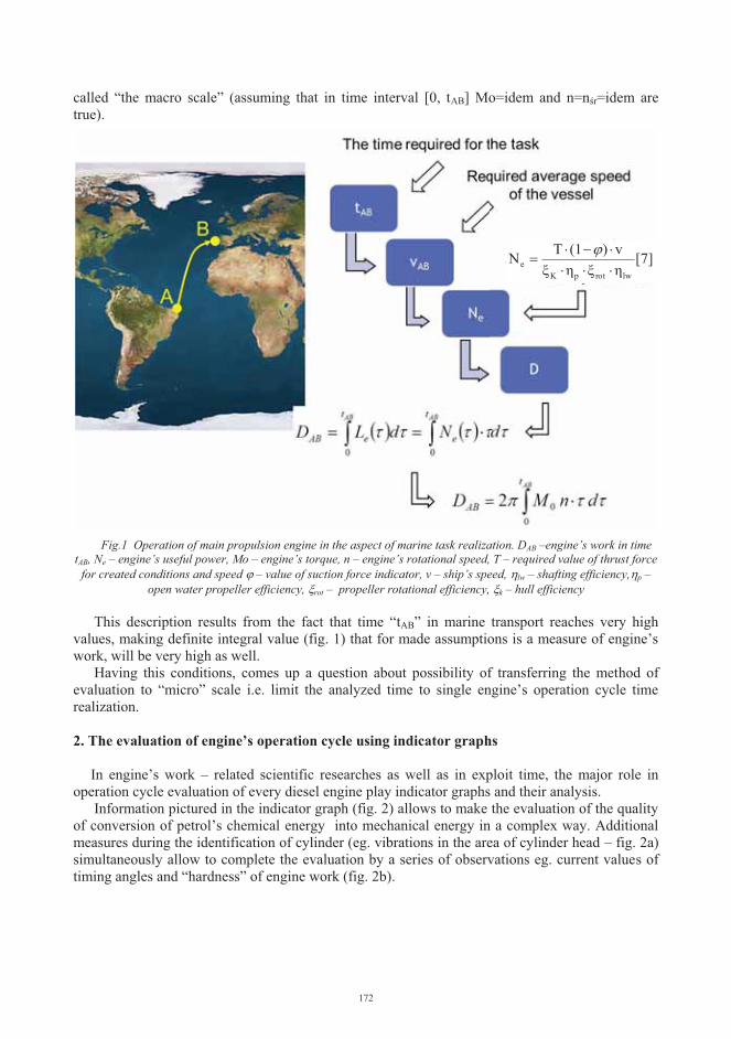
called “the macro scale” (assuming that in time interval [0, tAB] Mo=idem and n=nśr=idem are true).
Fig.1 Operation of main propulsion engine in the aspect of marine task realization. DAB –engine’s work in time tAB, Ne – engine’s useful power, Mo – engine’s torque, n – engine’s rotational speed, T – required value of thrust force
for created conditions and speed � – value of suction force indicator, v – ship’s speed, �lw – shafting efficiency,�p –open water propeller efficiency, >rot – propeller rotational efficiency, >k – hull efficiency
This description results from the fact that time “tAB” in marine transport reaches very high values, making definite integral value (fig. 1) that for made assumptions is a measure of engine’s work, will be very high as well.
Having this conditions, comes up a question about possibility of transferring the method of evaluation to “micro” scale i.e. limit the analyzed time to single engine’s operation cycle time realization.
2. The evaluation of engine’s operation cycle using indicator graphs
In engine’s work – related scientific researches as well as in exploit time, the major role in operation cycle evaluation of every diesel engine play indicator graphs and their analysis.
Information pictured in the indicator graph (fig. 2) allows to make the evaluation of the quality of conversion of petrol’s chemical energy into mechanical energy in a complex way. Additional measures during the identification of cylinder (eg. vibrations in the area of cylinder head – fig. 2a) simultaneously allow to complete the evaluation by a series of observations eg. current values of timing angles and “hardness” of engine work (fig. 2b).
]7[ηξηξv)(1TN
lwrotpKe ���
����
�
172

Fig.2 The engine’s extended indicator graph. p(�) – pressure as a function of crankshaft rotation, a(�) –accelerations of a cylinder head in the area of inlet valve, SI – the beginning of injection, IO – the beginning of the
opening of inlet valve
The analysis of data received in particular time, allows to calculate some more important work indicators, eg. mean indicated pressure – pi (fig. 3a) and indicated power – Ni (fig. 3b) in relation to all cylinders of the engine.
a)
b)
p(�)
a(�)
SIIO
173

Fig.3 Values of mean indicated pressure (MIP) and indicated power (PIND) for specific cylinders of 6 – cylinder engine.
These additional information about the values of pi and Ni in particular moment t, are necessary for predicting both future values of these indicators in time interval [t, t+�t] and estimation of the interval length.
Analysis of values and deviations from the mean of these, and others (eg, the maximum combustion pressure) quantities allows a fairly good comment on the quality of the implementation of energy transformation process.
On the one hand, it seems, therefore, that there is no need to introduce further parameters that would serve the present evaluation. On the other hand, each assessment and analysis, which is based on a larger number of variables is more complete and leads to more appropriate expertise and the resulting decisions.
As indicated earlier, further discussed among others in the works [4, 5, 6], quantitative assessment of the engine work using the D(t) indicator creates the possibility of another study examining the results of the research presented, it seems appropriate that the quantitative description of the engine work in macro scale time be extended on processes (on the same engine)on a scale "micro". In this case possible effects of DM(t) can be also distinguished and the action required by DW(t) of the engine. It is obvious that if the inequality of DM(t) < DW(t), appears, the engine cannot operate reliably in time t.
This seems all the more evident that the source of engine torque is rapidly changing the piston power, which largely depends on the instantaneous change in pressure in the cylinder.
3. The evaluation of the diesel engine work cycle using quantitative description of the operation D(t)
Because engine work is identified with physical quantity D(t) defined as [2]:
� �:�t
dtEtD0
)( ; (1)
where: D(t) – operation in time [0, t], E(;) – energy changeable in time eg. in the form of work,t – analyzed time,
and task execution time in the marine transport can be measured in hours, processing cycle scale of the work (even low-speed engines) requires:
� change the upper limit of integration in equation (1) for the duration of a cycle – t1ob, � a decision which component-associated quantity of the actual cycle can be considered as
time-variable energy according to equation (1).
174

The first of the above problems, of course, does not pose any difficulties since, in accordance with generally known that the time dependence can be expressed as [8]:
ntt obrob
LL ��� 11 (2)
where: t1ob – time of a one working cycle, t1obr – time of a one rotation of a crankshaft,
n – engine’s rotational speed,M - engine’s type factor (M = 1 – two-stroke engines, M = 2 – four-stroke engines),
The issue of choice of the value that corresponds to energy variable in time can raise some doubts, because the very concept of energy, as the scalar quantity describing the state of the system creates a rather wide possibilities of interpretation.
In the context of earlier analyzed results of cylinder inner pressures and opportunities of their presentation in the coordinate system p - V (volume - pressure), it seems appropriate to examine the work (a form of energy transfer), as a searched quantity.
Adoption of the convention allows for the transformation of equation (1) to the form:
� � � �:: ��obob tt
ob dtLdtED11
001 ;; (3)
where: D1ob – engine’s operation during one cycle, L(;) – cycle’s work up to the ; moment,
Dependence (3) follows from the fact that the value of work L is equal to the energy E, which was worn on the execution of this work.
Limiting to the concept of absolute work [3] and assuming the contractual rule that the work done by the working factor has a positive sign, and the work associated with the impact of environment on the factor - a negative sign, a work of a two-stroke engine during a operation cycle, or during the successive moments of duration of this cycle, can be determined by solution to the following equations:
� compression stroke - the work is done on the working factor (by convention, a negative sign), which can be interpreted as "negative" operation of engine - the need to provide energy:
o operation analyzed during the whole stroke:
� � � �: :: ���
!!"
#��
2
0
2
0
12
1
1 obob tV
V
t
CS dtdVVpdtLD ; , (4)
o operation analyzed as a function of time – time in the interval :
� � � �: ::22
���
!!"
#��
2
0
2
0
1
2
1
1
)(
obob tt V
V
tt
CS dtdVVpdtLtD ; , (5)
� the expansion and decompression stroke - the work is done by the working factor (by convention, a positive sign), which also can be interpreted as "positive" operation of the engine
o operation analyzed during the whole stroke:
175

� � � �: :: ���
!!"
#��
ob
ob
ob
ob
t
t
V
V
t
tES dtdVVpdtLD
1
1
1
2
1
122
; , (6)
o operation analyzed as a function of time – time in the interval :
� � � �: ::22
���
!!"
#��
ob
ob
ob
ob
tt
t
V
V
tt
tES dtdVVpdtLtD
1
1
1
2
1
122
)( ; (7)
� engine’s operation during the whole cycle
� � � �: :: : ���
!!"
#��
��
!!"
#���
2
02
12
1
1
1
1
2
obob
ob
tV
V
t
t
V
VCSESCS dtdVVpdtdVVpDDD (8)
Dependencies above can also be represented graphically in the form of the following procedure (Fig. 4 - 6):
Fig.4 Closed engine indicator graph. LE – expansion work, LC – compression work, LI –indicated work
Fig.5 Dependence of work and pressure during compression and expansion strokes. LE(t) –expansion work until the t moment, tC , LC(t) – compression work until the t
moment, tC
LE
LC
LI = LE - LC
p(t)
LC(t)
LE(t)
V2 V1
176

Rys.6 Określenie działania DCS(t) i DES(t) silnika w czasie suwów sprężania i rozprężaniawynikającego z prac Lc(t) oraz Le(t). DES(t) – działanie silnika w czasie suwu rozprężania do
chwili t, tC , DCS(t) – działanie silnika w czasie suwu sprężania do chwili t,
tC
The analysis (especially from functional process LC = f1(t) and LE = f2(t)) shows that the analysis and assessment of these types of work must be done with reference to the time of their implementation. This implies the need for research of engines during the dynamic time, which is the load compression and exhaust gas expansion time in each cylinder.
From the analysis of dependences (4) – (8) and pictures 4 – 6, following conclusions arise: � periodicity of compression and decompression processes prevents a simple analysis of the
engine (during time limited to t1ob) as a function of time. Such an analysis, is not impossible, but requires an additional, secondary index that takes into account the number of compression and expansion strokes executed up to the moment t,
� the value of engine operation at the time the operation cycle should be analyzed (in this case two - stroke engine) separately for compression and expansion stroke,
� separation of evaluation of cases of compression and expansion strokes allows accurate evaluation of their progress at any time, eg. in relation to the theoretical (pV� - idem) the implementation of these changes. This indicator can be defined as follows (eg. compression stroke):
� � � �
� �� � :
: :
: :
: :2
��
2
2
2
�����
���
!!"
#
�
��
�
!!
"
#���
!!"
#�
���
!!"
#
��2
01
1111
2
0
2
0 11
2
0
1
1
1
1
1
1
1
1
)(')()(
ob
ob
t
ob
t
ob
t
tt
t
tt V
Vt
t V
V
t
tt V
V
CS
CS
dtV
VVp
dtdVVp
dtdVVVp
dtdVVp
tDtDt
�
�
�
���, (9)
gdzie: �(t) – engine’s operation evaluation indicator during the compression stroke (as a
function of time)DCS(t) – operation during the compression stroke in the real engine, D’CS(t) – operation during the compression stroke during the implementation of the
theoretical cycle
LC(t)
LE(t)
DES(;2)
DCS(;1)
DCS(t)
DES(t)
;2;1
177

p1 – pressure at the beginning of the compression stroke V1 – volume of working space in the piston BDCVt – volume of working space at the moment t (VTDC = V2 2 Vt 2 V1)� – isentrope exponent
� determination of the value of performance indicators - DCS and DCS(t) for the reference state, ie. a new engine capable of full technical efficiency and fitness, allows for ongoing evaluation of the quality of the implementation cycle (in this case compression). This can be illustrated as shown below (Fig. 7), which presents a two processes of compression job instantaneous values LC (t) – for a reference state and in case of excessive leakage in the piston - cylinder system – L”C (t) and the corresponding change in action compression stroke time - DCS (t) and D”CS (t).
Fig.7 Engine operations in the time of compression strokes for an engine in the reference technical state -DCS(t) and in case of excessive use of piston – cylinder system elements - D”CS(t). LC(t) – compression work up to the t moment (reference engine), L”C(t) – compression work p to the t moment (engine in the state of
technical inefficiency of piston – cylinder system), tCSimilarly the size of LE (t) and the LE '(t) and DES (t) and DES' (t) can be determined, where LE (t) and DES (t) are illustrated in figure 6
Regardless of the proposed method of the evaluation performance of the engine in the so-called the dynamic (short) time, this activity can be seen in the reliability having possible action DCS(M)(t) and DES(M)(t) as well as required action DCS(W)(t) and DES(W)(t).
4. Summary
The proposed procedure when analyzing test results from diesel engine is an attempt to transfer an engine activity evaluation methods in the operational time scale (exploit time), eg. in hours, to the micro-scale (dynamic time) relating only to the execution time of one (several) working cycles.
The presented method seems to be acceptable supplement for already used methods of realization of operation cycle in diesel engine evaluation. Its possible usefulness requires, of course, further theoretical studies and research supplies. In view of the fact that the induction of marine engines is a common and general routine operating practice, access to the results of such
DCS(t)
D”CS(t)
LC(t)
L”C(t)
178

studies is quite easy, and thus conducive to the development of the presented evaluation method tools.
The basic advantage of this method is the link between evaluation of the work and the time the task is done - in this case during operation cycle of the engine.
Not without significance is the fact that all the necessary calculations are relatively simple and can be made only on the basis of the indicator graph received. The development of modern electronic indicators, so called pressure analyzers, allows for seamless implementation of these calculations in the software environment of such a device
The practical usefulness of the results obtained at the present time may be questionable - butfurther empirical studies of piston engines operation understood this way can lead to practical application of the proposed method of performance evaluation of such engines.
References
1 Girtler J., Kuszmider S., Plewiński L., Wybrane zagadnienia eksploatacji statków morskich w aspekcie bezpieczeństwa żeglugi, Monografia, WSM, Szczecin 2003.
2 Girtler J., A Method for Evaluating the Performance of a Marine Piston Internal Combustion Engine Used As the Main Engine on a Ship During Its Voyage in Different Sailing Conditions, Polish Maritime Research, No 4(67), Vol 17, Gdańsk 2010.
3 Ochęduszko S., Termodynamika stosowana, WNT, Warszawa1970. 4 Rudnicki J., Działanie systemu energetycznego w ujęciu wartościującym z uwzględnieniem
jego struktury niezawodnościowej oraz stopnia zużycia potencjału użytkowego. Praca wykonana w ramach projektu finansowanego przez MNiSW Nr N509 045 31/3500. Projekt badawczy pt., „Kształtowanie bezpieczeństwa działania systemów energetycznych środków transportowych na przykładzie systemów okrętowych”, Gdańsk, 2008.
5 Rudnicki J., Quantitative Assessment of Operation of Ship Main Diesel Engine, InternationalConference on Computational Methods in Marine Engineering, MARINE 2011 CIMNE, Lisbona 2011.
6 Rudnicki J., Loads of Ship Main Diesel Engine in the Aspect of Practical Assessment of Its Operation, Journal of Polish CIMAC, Vol. 3, No 1, Gdańsk 2008.
7 Urbański P., Podstawy napędu statków, Wyd. Fundacji Rozwoju Akademii Morskiej, Gdynia 2005.
8 Wajand J.A., Silniki o zapłonie samoczynnym, WNT, Warszawa 1988.
179

180

Possibility of Improvement of Some Parameters of Dual Fuel CI Engine by Pilot Dose Division
Zdzislaw Stelmasiak
Technical University of Bielsko-Biala, Internal Combustion Engines and Automobiles Branch
ul. Willowa 2, 43-300 Bielsko-Biała, Poland
Abstract
The paper present a test results of dual fuel engine run on natural gas and diesel oil injected as a pilot dose. Determination of possibilities of engine’s operational parameters improvement through division of the pilot dose was the main objective of the presented research. The first dose injected at ignition advance angle, the same as in case of operation on diesel oil only, has as its task to initiate process of combustion. The second dose, injected with changing delay when, as assumed, phase of combustion process is already in progress, has as its task to sustain combustion of gaseous mixture. Control of combustion process was attained through changes of injection delay angle of additional dose. Division of pilot dose effects in a considerable reduction of maximal heat release rate during combustion with simultaneous growth of average combustion rate of gas-air mixture. In result, it has been observed a growth of overall efficiency of the engine, reduction of NOx concentration in exhaust gases, and reduction of maximal combustion pressures. Simultaneously, emission of the CO and TCH was slightly worsened.
Keywords: natural gas, dual fuel engine, pilot dose, thermal efficiency, combustion parameters
1. Introduction
Nowadays, a search after alternative fuels suitable to internal combustion engines is observed in more and more extent. One from such fuels are various type gaseous fuels like: natural gas, biogas, by-product gases from manufacturing processes. Engines run on gas can operate according to two systems of combustion:
� spark ignition system (majority of applications), � dual fuel system (limited number of applications).
In past, selection of such system was determined by considerable differences in price of the fuels mainly; by-product gases having low price of elementary energy and diesel oil with high unit costs. With considerable portion of diesel oil, cost of production of elementary energy in dual fuel engines was higher than production cost of energy in spark ignition engines. Difficulties in mechanical control of fuel charge quality in dual fuel engine constituted additional problem. In result, spark ignition engines can be found in majority of practical applications. This system requires, however, reduction of compression ratio to values of about � = 9,0÷9,5, what results in reduction of thermal efficiency, comparing to compression ignition engines fueled traditionally (Fig. 1).
181

In dual fuel engine, to the cylinder is sucked in homogenous gas-air mixture, ignited due to injection of small pilot dose of diesel oil. Energetic fraction of diesel oil depends on implemented feeding system and size of engine, and can change in the following range:
� 1,5÷3,0% - the best stationary duel fuel engines with high power outputs, � 3,0÷5,0% - generator type dual fuel engines with power outputs above 2 MW, � 5,0÷10,0% - dual fuel engines with power outputs < 500 kW, � 15,0÷30,0% - compression ignition engines adapted to dual fuel feeding.
0 20 40 60 80 100Engine load [%]
0
10
20
30
40
50
Ther
mal
eff
icie
ncy
[%]
CI - DO190 kW
SI - CNG190 kW
SI-CNG165 kW
Fig. 1. Comparison of thermal efficiency of SI gaseous engines and CI engines fuelled traditionally [1]
The most advantageous conditions to combustion of gas in dual fuel engines are present near the point of maximal load. In such case the engine can be run on rich mixture with excess air ratio of �g=1,5�2,0, characteristic of high combustion rate. As a rule, in such case the dual fuel engine features thermal efficiency higher than an engine run on diesel oil only.
One from the main problems of the dual fuel engines is reducing thermal efficiency at partial loads. It is connected with leaning of combustible mixture and worsening conditions of its combustion. When pilot doses are small, nearly entire liquid fuel evaporates during delay of self-ignition. Combustion time of pilot dose is very short and combustion runs violently. Good conditions of ignition and combustion are in the layer of gas-air mixture adhering to burning stream of liquid fuel. As combustion process of liquid fuel fades away, and front of flame recedes from the stream, combustion process runs more and more slowly. Cooling effect of cylinder walls has also disadvantageous effect here. At lean gas-air mixtures a fading of the flame can occur, what can have effect on efficiency and ecological parameters of the engine.
The main objective of the present work was to investigate a possibility of elicitation of combustion of gas-air mixture through division of pilot dose. Such possibility is offered by modern injection systems of Common Rail type, commonly used in contemporary compression ignition engines. In course of performed tests, dose of diesel oil was divided into two equal parts injected in different time. The first dose injected with ignition advance angle, the same as in case of operation on diesel oil only, had its task to initiate combustion process. The second dose, injected with changing delay when, as assumed, phase of combustion process is already in progress, had its task to sustain process of combustion of gaseous mixture. Control of combustion process was attained by changes of ignition delay angle of additional dose.
Division of pilot dose, according to assumption, should lead to change of heat release rate, what was confirmed by performed tests, see Fig. 2.
In the Fig. 2 is distinctly seen a change of heat release run for ignition generated by divided pilot dose. Additional dose of diesel oil effects in generation of the second maximum
182

on the heat release curve, with its value considerably higher than the first maximum. It can prove about growth of active combustion rate of gaseous mixture. Simultaneously, maximal values of heat release rate are smaller than the ones present during combustion of charge with single dose. It augurs well for process of NOx generation, especially in case of turbocharged engines.
n = 1200 rpm/minMo = 52,1 NmNww = 20oCA
pilot singledivided ��=10oCAdivided ��=15oCA
-20 0 20 40Crank Angle �[oCA]
0
4
8
12
16
dQ/d
� [M
J/km
ole.o
CA
] Mo = 72,9 Nm
-20 0 20 40Crank Angle �[oCA]
0
4
8
12
dQ/d
� [
MJ/
kmol
e.oC
A]
Mo = 52,1 Nm
Fig. 2. Comparison of heat release rate in the dual fuel engine with single and divided pilot dose
In the present paper is discussed an effect of division of pilot dose on a selected parameters of dual fuel engine.
2. Test stand
The tests were performed on single cylinder, compression ignited engine of SB3.1 type. Technical data of the engine are specified in the Table 1, while view of the test stand is shown in the Fig. 3. Detailed description of the test stand and modifications made in the engine can be found in earlier publications [1,2].
Table 1. Technical data of the SB3.1 engine
Cylinder number 1Bore 127 mmStroke 146 mmDisplacement volume 1848 cm3
Compression ratio 15,8Effective output power 22,8 kWRotational speed 2200 rpm/minCombustion chamber Direct injection to chamber
in piston crownInjection system of DO Common Rail f-my BoschInjector of DO Bosch 0986435 004 090Injection system of CNG ICGas injector Bosch F465 151 72Presser of gas injection 1 MPa
Fig. 3. Engine test bend
In course of performed tests one used constant ignition advance angle of 20oCA before TDC, the same like in case of run on diesel oil only. Division of the dose was accomplished by split of injector’s opening time in Common Rail system, ;ow, according to the following rule: opening time of the injector for pilot dose ;ow1 = 0,5;ow , for additional dose ;ow2 =0,5;ow. Performed earlier tests have revealed, that characteristic of injector output is exactly
183

linear, while size of injected dose is proportional to opening time of the injector. It has enabled to assume equity of pilot and additional doses; q1 = q2 = 0,5qon. Implemented controller has enabled recalculation of beginning of injection into angular values with respect to the TDC, what enables to maintain required values of injection advance angle of pilot dose Nww. Ignition delay of additional dose was also measured as angular value �α, calculated from beginning of injection of the first dose. It should be underlined, that at small values of the dwell, �α, electromagnetic injector can be not fully closed, what can have such effect that preset delay of the additional dose effects in modulation of intensity of injected fuel only.This assumption was confirmed by the tests performed on a test stand without engine. The modulation has an effect on course of engine operation, what was confirmed during testing on engine dynamometer and in results of numerical analysis of combustion parameters.
Analysis of combustion parameters was performed on base of thermal calculations based on recorded indicator diagrams. In course of the calculations one made use of author’s computer program developed in the Department of Internal Combustion Engines, University of Bielsko-Biala. Description of the program and methodology of the calculations can be found in the work [7, 8].
3. Analysis of the test results
In the Fig. 4 are presented runs of heat release rate in range of active combustion, from beginning of the process up to 50oCA after TDC. Runs for two rotational speeds 1200 and 1400 rpm (near point of maximal torque) and for two engine loads (maximal: when gas-air mixture is the richest, and minimal: with maximal leaning of gaseous mixture) were analyzed.
pilot single
divided ��=10oCA
divided ��=15oCA
-20 0 20 40Crank Angle �[oCA]
-4
0
4
8
12
16
20
dQ
/d�
[M
J/km
ole.
o CA
] 1200 rpm/minMo = 93,8 Nm
-20 0 20 40Crank Angle �[oCA]
-4
0
4
8
12
16
20
dQ
/d�
[M
J/km
ole.
o CA
] 1400 rpm/minMo = 93,8 Nm
-20 0 20 40Crank Angle �[oCA]
0
4
8
12
dQ
/d�
[M
J/km
ole.
o CA
] 1200 rpm/minMo = 31,3 Nm
-20 0 20 40Crank Angle �[oCA]
0
4
8
12
dQ/d
� [
MJ/
kmol
e.o C
A]
1400 rpm/minMo = 31,3 Nm
Fig. 4. Comparison of heat release rate in dual fuel engine with single and divided pilot dose
184

Analysis of the runs presented in the Fig. 4 is pointing at explicit changes in run of heat release depending on method of fuelling. In case of single fuel dose used, a single maximum is present. It results from rapid combustion of diesel oil in kinetic phase of combustion, evaporated during later self-ignition. After implementation of divided dosage, maximal value of heat release rate is nearly two-fold lower, and additionally shifted in direction of more late phases of combustion. In range of maximal engine load, rich gaseous mixture with high combustion rate, shift of maximum heat release is small, especially for delay of additional dose with �α=10oCA. This delay is growing with leaning of gaseous mixture (partial loads) and increasing of injection delay angle of additional dose. At partial engine loads, on the dQ/d� curve are distinctly present two maxima, what confirms assumption about combustion of the dosages in different time. In spite of equal sizes of injected doses, maximal dynamics of heat release distinctly decreases together with growth of injection delay angle of additional dose.
Usage of divided pilot dose effects in reduction of maximal combustion pressures as injection delay of additional dose of diesel oil grows, Fig. 5. Simultaneously, pressure’s run during initial phase of combustion is delayed comparing to the run with not divided dose. In consequence, point of maximal pressure is shifted in direction of more late angles after TDC. Character of described here pressure changes is present in whole range of engine load change. It should be underlined, however, that at partial engine loads, effect of the division and delay angle on initial phase of combustion is more distinct, what reveals a distinct inflexion of pressure line.
pilot single
divided ��=10oCA
divided ��=15oCA
-20 0 20 40Crank Angle �[oCA]
0
2
4
6
8
10
Cyl
inde
r Pre
ssur
e p
[M
Pa]
1200 rpm/minMo = 93,8 Nm
-20 0 20 40Crank Angle �[oCA]
0
2
4
6
8
10
Cyl
inde
r Pre
ssur
e p
[M
Pa]
1400 rpm/minMo = 93,8 Nm
-20 0 20 40Crank Angle �[oCA]
0
2
4
6
8
Cyl
inde
r Pre
ssur
e p
[M
Pa]
1200 rpm/minMo = 31,3 Nm
-20 0 20 40Crank Angle �[oCA]
0
2
4
6
8
Cylin
der p
ress
ure
[MPa
]
1400 rpm/minMo = 31,3 Nm
Fig. 5. Comparison of cylinder pressure in dual fuel engine with single and divided pilot dose
185

Maximal values of the pressure and heat release rate during combustion in function of engine load are presented in the Fig. 6. Values of the both analyzed parameters, when the pilot dose is divided, are smaller. Especially brings our attention a significant reduction of maximal value of the heat release rate, (dQ/d�)max. In range of maximal engine load, the reduction is 2,0÷2,5 fold, while at minimal loads with 25÷40%. It is also worth to underline, that in case of division of pilot dose, the same engine loads are developed at a lower maximal pressures, what can have effect on growth of durability of crankshaft system, especially bearings.
pilot single
divided ��=10oCA
divided ��=15oCA
20 40 60 80 100 Mo [Nm]
5
6
7
8
9
10
p max
[M
Pa]
1200 rpm/min
20 40 60 80 100Mo [Nm]
5
6
7
8
9
10
(dQ
/d�
) max
[M
J/km
ole.o
CA]
1400 rpm/min
20 40 60 80 100 Mo [Nm]
2
4
6
8
10
12
(dQ
/d�
) max
[M
J/km
ole.o
CA
]
1200 rpm/min
20 40 60 80 100Mo [Nm]
2
4
6
8
10
12
(dQ
/d�
) max
[M
J/km
ole.o
CA]
1400 rpm/min
Fig. 6. Comparison of maximal combustion parameters in dual fuel engine SB3.1 with single and divided pilot dose: pmax – maximal value of cylinder pressure, (dQ/d�)max – maximal value of heat release rater
Division of pilot dose results in growth of engine efficiency with 1,0�3,5% of absolute units. More advantageous results were obtained at smaller injection delay angle of additional dose. Differences in analyzed values of the efficiency are also dependant on rotational speed. Increase of injection delay angle of additional dose effects adversely on efficiency of the engine, reducing differences between values of the efficiency for non split dose and divided dose. However, it is worth to underline, that for the both tested angles of injection delay, 10 and 15oCA, the engine operated with a higher efficiency than in case observed with not split pilot dose. Absolute increase of engine efficiency with 1,0�3,5% is pointing at distinct relative differences of the efficiency. They amount to 10�15% for engine speed of 1200 rpm and 8�10% for engine speed of 1400 rpm. Such meaningful growth can prove about considerable reduction of energy consumption by the engine operating at changing conditions of load.
Division of pilot dose, resulted in described earlier change of combustion run, advantageously effects on concentration of NOx in exhaust gases, decreasing considerably as
186

injection of additional dose is delayed, Fig. 8. It results from two main reasons, reduction of maximal temperatures in zones of oxidation of liquid fuel, and reduction of oxidation rate in zones with a higher concentrations of carbon dioxide (additional dose undergoes oxidation in conditions of increased EGR).
pilot single
divided ��=10oCA
divided ��=15oCA
20 40 60 80 100Mo [Nm]
10
20
30
40
50
Ther
mal
Eff
icie
ncy
[%] 1200rpm/min
20 40 60 80 100Mo [Nm]
10
20
30
40
50
Ther
mal
Eff
icie
ncy
[%] 1400 rpm/min
Fig. 7. Comparison of thermal efficiency in dual fuel engine with single and divided pilot dose
pilot single
divided ��=10oCA
divided ��=15oCA
20 40 60 80 100Mo [Nm]
0
500
1000
1500
2000
2500
3000
NO
x [
ppm
]
1200 rpm/min
20 40 60 80 100Mo [Nm]
0
1000
2000
3000
4000
NO
x [
ppm
]
1400 rpm/min
20 40 60 80 100Mo [Nm]
0
400
800
1200
1600
TCH
[p
pm]
1200 rpm/min
20 40 60 80 100Mo [Nm]
400
800
1200
1600
2000
CO
[ppm
]
1200 rpm/min
Fig. 8. Comparison of concentration of toxic exhaust components the dual fuelled engine SB3.1with single and divided pilot dose
Reduction of oxygen concentration in zones of the reaction, caused by partial burn-out of the fuel, can also have additional effect. Observed changes in concentration of NOx suggest,
187

that condition of oxidation of liquid fuel can have significant effect on emission of nitrogen oxides in dual fuel engines. Simultaneously, obtained results in range of NOx concentrations confirm that division of the pilot dose and correctly selected injection angle of additional dose can serve as a substantial tool to reduction of nitrogen oxides emission in highly supercharged dual fuel engines. It should be emphasized in this point, that reduction of NOx concentration was obtained together with simultaneous growth of overall efficiency of the engine, what – asseen from previous tests – is not possible with single pilot dose.
Delay in injection of diesel oil slightly increases concentrations of carbon oxide, CO, and total amount of hydrocarbons, TCH, (Fig. 8). It results from worsening of conditions of liquid fuel oxidation in more late phases of combustion. It is distinctly confirmed by differences in concentration of CO and THC for delay angles of 10 and 15oCA. Slight growth of concentrations of CO and TCH does not create a problem in contemporary engines due to high conversion efficiency of oxidation catalysts. Moreover, concentrations of CO downstream the exhaust valve (before the catalyst) are smaller, with order of magnitude, from concentration of CO in case of gaseous engines with spark ignition.
4. Conclusions
Based on performed tests it is possible to formulate the following general conclusions: � Division of pilot dose and changes in parameters of the doses are nowadays easy to be
accomplished in compression ignition engines due to high pressure Common Rail injection systems, commonly used in the engines.
� The tests have shown that division of diesel oil dose in dual fuel engines leads to changes in combustion course of gaseous mixture. It is especially visible at partial engine loads, when the gas-air mixture is excessively leaned.
� Division of pilot dose can be accomplished only in dual fuel engines operated at a bigger energetic share of diesel oil. It is connected with possibilities of injection of very small doses of liquid fuel. Division at small portions of diesel oil requires incorporation of additional injector for pilot doses, what increases cost of engine adaptation to dual fuel feeding.
� To advantageous phenomena connected with division of the dose belong: absolute growth of overall efficiency of the engine with 1,0÷3,5% (8÷15% of relative growth), reduction of NOx emission in exhaust gases and more quiet and less noisy engine operation. Among adverse phenomena can be counted: a slight growth of CO and TCH emissions and when inappropriate injection parameters of additional dose were selected, possibility of growth of engine’s thermal load.
REFERENCES
1. Stelmasiak Z., Larisch J., Gilowski T., Matyjasik M.: Możliwości poprawy składu mieszaniny gazowej przez dławienie powietrza przy częściowych obciążeniach silnika dwupaliwowego, Archiwum Motoryzacji 1/2007, str. 43-57, 2007.
2. Stelmasiak Stelmasiak., Larisch J., Gilowski T.: Możliwości sterowania dawką inicjującą oleju napędowego w dwupaliwowych silnikach ZS wyposażonych w system Common Rail, PTNSS Kongres – 2005, Szczyrk 25-28.09.2005, Paper No. PTNSS P05-C004,2005.
3. Stelmasiak Z.: Analiza wpływu składu mieszaniny gaz-powietrze na parametry dwupaliwowego silnika o wtrysku bezpośrednim, Silniki Spalinowe nr 3/2005.
4. Friedeman Z.: Gasmotoren, Vogel Buchverlag, Würzburg, 2001.
188

5. Zua CH., Zhao J.: Development of Diesel Engines Fuelled with Natural Gas, SAE Paper No. 2001-01-3505, 2001.
6. Clark N.N., Atkinson Chr.M., Atkinson R.J., McDaniel T.I., ParkT.: Optimized Emission Reduction Strategies for Dual Fuel Compression Ignition Engines Running on natural Gas and Diesel. www.cemr.wvuedu/-englab/project/navistar.html, 2002.
7. Stelmasiak Z.: Analysis of Combustion Phenomena in Dual Fuel Engine Fed With Natural Gas (CNG). Fisita 2002 World Automotive Congress, Paper No. F02 V030, 2002.
8. Stelmasiak Z.: Studium spalania gazu w dwupaliwowym silniku o zapłonie samoczynnym zasilanym gazem ziemnym i olejem napędowym, Wydawnictwo ATH, nr 5/2003.
189

190

INFLUENCE OF THE SERVICE MARGIN OF SERVICE PARAMETERS OF TRANSPORT SHIP PROPULSION SYSTEM
Part I
Propulsion engine service parameters of transport ship sailing on a given shipping route
Tadeusz Szelangiewicz, Katarzyna Żelazny
Westpomeranian University of Technology in Szczecin, Faculty of Maritime Technology and Transport, Piastów 41, 71-065 Szczecin, Poland
tel. +48 91 449 41 26, fax: +48 91 449 46 95 e-mail: [email protected], [email protected]
Abstract
During ship sailing on a given shipping route in real weather conditions all propulsion system performance parameters of the ship change along with changes of instantaneous total resistance and speed of the ship. In this paper results of calculations are presented of distribution function and mean statistical values of screw propeller thrust, rotational speed and efficiency as well as propulsion engine power output and specific fuel oil consumption occurring on selected shipping routes at different SM values. On this basis new guidelines for ship propulsion system design procedure are formulated.
Keywords: thrust, efficiency and rotational speed of screw propeller, long-term prediction, shipping route, design working point of screw propeller, service margin
1. Introduction
A crucial element of a design process of a transport ship propulsion system is the selection of its design parameters, i.e. determination of a speed value for which screw propeller should be designed and determination of a thrust value which should be developed by this propeller at the assumed speed. Correct selection of the design speed is specially important for ships fitted with fixed pitch propellers (most often applied to transport ships) as only at that design speed such propeller is able to use full engine power output.
The service speed at which the designed ship has to operate in real weather conditions on a given shipping route, should be assumed as the design speed.
The way of calculation of the mean long-term service speed and the mean long-term resistance of the ship is presented in [1,2,3]
191

The design working point of screw propeller is associated with the following design parameters: ship speed and propeller thrust. Selection of such point is very important with a view of correct operation of propulsion system. In this point screw propeller efficiency should reach as - high - as possible value. For screw propellers interacting with piston combustion engines the design point is usually placed half way between the points A and B (Fig. 1), that generally ensures correct operation of the propulsion system in the point B, i.e. in service conditions (real weather conditions). The characteristic crossing point A (Fig 1) is determined on the basis of the ship resistance on still water, while characteristic crossing point B is determined while taking into account additional resistance values of wind and waves. As a standard characteristic results from the addition of 15% SM to characteristic . As demonstrated in publications [1], [2], [3] such SM value is offen to small to establish a mean statistical service speed of ship on numerous sailing routes with adequate probability (i.e. eg. 95%) Instantaneous service speed of a ship and its total resistance depend on instantaneous weather conditions occurring on a given shipping route. Hence working parameters of the screw propeller designed and applied to propel the ship will be changeable depending on weather parameters and assumed criteria of propulsion system control [4]. Knowing statistical data on wind and waves occurring on a given shipping route as well as long-term distribution function of ship speed [3] on the route, one can determine long-term distribution functions of working parameters of the screw propeller and hence mean statistical location of its working point on a given shipping route.
The working parameters of the propeller and the overall propulsion system depend also on the adopted SM value
Fig. 1. Predicted service speed of ship Pn – nominal power output of engine, PS – shaft-line power, PD – power delivered to propeller cone, VK – contractual
speed of ship, VE – predicted service speed of ship, 1 – still-water propeller curve for clean ship hull, 2 – predicted propeller curve with service margin, in real conditions, OM – operational margin, SM – service margin, �PS – power loss
at shaft-line (and possibly… if used)
Therefore this paper presents calculations - performed for a designed ship – of long-term service parameters of screw propeller and mean service location of its working point as well as a discussion on how these would influence the ship’s design working point at different values of service margin
21
Ship speed
VE VK
A
B
B’
Pn
OMPS
SM
Prop
ulsi
on sy
stem
pow
er o
utpu
t
2
1
PD
�PS
192

2. Service parameters of screw propeller
The service parameters of screw propeller to be calculated for a ship sailing on a given shipping route are the following: O the propeller thrust T,O the propeller rotational speed np,O the free-propeller efficiency η0 .
The propeller thrust T with the propeller situated behind a ship’s hull is calculated for the total resistance CR of a ship sailing through waves at assumed service speed VE with a given geometry of a screw propeller (mathematical model adopted to calculate the propeller thrust is presented in [1], [2], [3]). In calculations of thrust, its fall resulting from sailing on waves was taken into account [5].
The engine speed np transmitted on the screw cone and its torque Q while sailing through waves on a given shipping route [1], [2], [3], and open water propeller efficiency 0� , is presented by the equation:
��
20J
KK
Q
T �� (1)
where: KT – propeller thrust ratio, KQ – propeller torque ratio, J – advance ratio.
3. Mean statistical values of screw propeller service parameters of ship sailing on a given route
The calculation of mean statistical values of screw propeller service parameters were performed according to the algorithm shown in [2], [3] or [5], for ship M2 (whose parameters are given in [3]), for different sailing routes [3] and propelling engines whose nominal power was determined at 15% SM (a standard value adopted during the M2 design procedure) and then SM = 20% and 25%.
Results of the calculations for the selected ship and its shipping routes are presented in the form of : • histogram of propeller thrust and its mean statistical value• histogram of propeller speed and its mean statistical value• histogram of propeller efficiency and its mean statistical value • mean statistical propeller working point,• probability distribution function of long-term occurrence of given values of propeller rotational
speed and ship service speed.
All the calculations were performed under the assumption that engine’s power output reaches at most 0.9 Pn.
In the below attached figures the calculation results are presented for K1 containership [3] on two very different shipping routes: 5b - “easy” one and 2b - „difficult” one – in the sense of occurrence oflong-term weather parameters.
The results of the calculations are presented in Fig. 2 � 6 and a summary table 1.
193

Ship: M2 - assumed service speed = 7,72 [m/s] SM=15%- probability of maintaining the assumed speed PVE
Route no. 2b - PVE = 0,55 Route no. 5b - PVE = 0,86Thrust histograms
0
0,1
0,2
0,3
0,4
0,5
0,6
0,7
0,8
0,9
1
35,1
87,7
122,
8
157,
9
193,
0
228,
1
263,
1
298,
2
333,
3
368,
4
403,
5
438,
6
473,
7
508,
7
543,
8
578,
9
614,
0
649,
1
684,
2
719,
3
754,
4
789,
4
Thrust on still water T= 737 [kN]Mean thrust T = 752 [kN]
0
0,1
0,2
0,3
0,4
0,5
0,6
0,7
0,8
0,9
1
35,1
87,7
122,
8
157,
9
193,
0
228,
1
263,
1
298,
2
333,
3
368,
4
403,
5
438,
6
473,
7
508,
7
543,
8
578,
9
614,
0
649,
1
684,
2
719,
3
754,
4
789,
4
T [kN]Mean thrust T = 741 [kN]
Propeller histograms
0
0,1
0,2
0,3
0,4
0,5
0,6
0,7
0,8
0,9
1
0,34
2
0,72
2
0,79
7
0,87
2
0,94
7
1,02
2
1,09
7
1,17
2
1,24
7
1,32
3
1,39
8
1,47
3
1,54
8
1,62
3
1,69
8
1,77
3
1,84
8
1,92
3
1,99
9
2,07
4
Nominal propeller speed nn= 2,030 [1/s]Mean propeller speed n = 2,021 [1/s]
0
0,1
0,2
0,3
0,4
0,5
0,6
0,7
0,8
0,9
1
0,34
2
0,72
2
0,79
7
0,87
2
0,94
7
1,02
2
1,09
7
1,17
2
1,24
7
1,32
3
1,39
8
1,47
3
1,54
8
1,62
3
1,69
8
1,77
3
1,84
8
1,92
3
1,99
9
2,07
4
n[1/s]Mean propeller speed n = 2,031 [1/s]
Propeller efficiency histograms
0
0,1
0,2
0,3
0,4
0,5
0,6
0,7
0,8
0,9
1
0,01
5
0,04
5
0,07
6
0,10
6
0,13
6
0,16
6
0,19
6
0,22
7
0,25
7
0,28
7
0,31
7
0,34
7
0,37
8
0,40
8
0,43
8
0,46
8
0,51
4
0,52
9
0,55
9
0,58
9
Propeller efficiency in still water �0= 0,513Mean propeller efficiency � 0= 0,499
0
0,1
0,2
0,3
0,4
0,5
0,6
0,7
0,8
0,9
1
0,01
5
0,04
5
0,07
6
0,10
6
0,13
6
0,16
6
0,19
6
0,22
7
0,25
7
0,28
7
0,31
7
0,34
7
0,37
8
0,40
8
0,43
8
0,46
8
0,51
4
0,52
9
0,55
9
0,58
9
�0 [-]Mean propeller efficiency � 0= 0,510
Fig. 2. Histograms and mean statistical values of thrust, propeller speed and efficiency of an M2 ship on sailing routes 2b and 5b (SM = 15%)
PTT
PTn
PT�
194

Ship: M2 - assumed service speed = 7,72 [m/s] SM=20%- probability of maintaining the assumed speed PVE
Route no. 2b - PVE = 0,79 Route no. 5b - PVE = 0,96Thrust histograms
0
0,1
0,2
0,3
0,4
0,5
0,6
0,7
0,8
0,9
1
35,1
87,7
122,
8
157,
9
193,
0
228,
1
263,
1
298,
2
333,
3
368,
4
403,
5
438,
6
473,
7
508,
7
543,
8
578,
9
614,
0
649,
1
684,
2
719,
3
754,
4
789,
4
Thrust on still water T= 737 [kN]Mean thrust T = 785 [kN]
0
0,1
0,2
0,3
0,4
0,5
0,6
0,7
0,8
0,9
1
35,1
87,7
122,
8
157,
9
193,
0
228,
1
263,
1
298,
2
333,
3
368,
4
403,
5
438,
6
473,
7
508,
7
543,
8
578,
9
614,
0
649,
1
684,
2
719,
3
754,
4
789,
4
T [kN]Mean thrust T = 752 [kN]
Propeller histograms
0
0,1
0,2
0,3
0,4
0,5
0,6
0,7
0,8
0,9
1
0,34
7
0,73
1
0,80
8
0,88
4
0,96
0
1,03
6
1,11
2
1,18
8
1,26
4
1,34
0
1,41
6
1,49
3
1,56
9
1,64
5
1,72
1
1,79
7
1,87
3
1,94
9
2,02
5
2,10
2
Nominal propeller speed nn= 2,057 [1/s]Mean propeller speed n = 2,063 [1/s]
0
0,1
0,2
0,3
0,4
0,5
0,6
0,7
0,8
0,9
1
0,34
7
0,73
1
0,80
8
0,88
4
0,96
0
1,03
6
1,11
2
1,18
8
1,26
4
1,34
0
1,41
6
1,49
3
1,56
9
1,64
5
1,72
1
1,79
7
1,87
3
1,94
9
2,02
5
2,10
2
n[1/s]Mean propeller speed n = 2,045 [1/s]
Propeller efficiency histograms
0
0,1
0,2
0,3
0,4
0,5
0,6
0,7
0,8
0,9
1
0,01
5
0,04
5
0,07
6
0,10
6
0,13
6
0,16
6
0,19
6
0,22
7
0,25
7
0,28
7
0,31
7
0,34
7
0,37
8
0,40
8
0,43
8
0,46
8
0,51
4
0,52
9
0,55
9
0,58
9
Propeller efficiency in still water �0= 0,513Mean propeller efficiency � 0= 0,499
0
0,1
0,2
0,3
0,4
0,5
0,6
0,7
0,8
0,9
1
0,01
5
0,04
5
0,07
6
0,10
6
0,13
6
0,16
6
0,19
6
0,22
7
0,25
7
0,28
7
0,31
7
0,34
7
0,37
8
0,40
8
0,43
8
0,46
8
0,51
4
0,52
9
0,55
9
0,58
9
�0 [-]Mean propeller efficiency � 0= 0,510
PTT
PTn
PT�
Fig. 3. Histograms and mean statistical values of thrust, propeller speed and efficiency of an M2 ship on sailing routes 2b and 5b (SM = 20%)
195

Ship: M2 - assumed service speed = 7,72 [m/s] SM=25%- probability of maintaining the assumed speed PVE
Route no. 2b - PVE = 0,82 Route no. 5b - PVE = 0,97Thrust histograms
0
0,1
0,2
0,3
0,4
0,5
0,6
0,7
0,8
0,9
1
35,1
87,7
122,
8
157,
9
193,
0
228,
1
263,
1
298,
2
333,
3
368,
4
403,
5
438,
6
473,
7
508,
7
543,
8
578,
9
614,
0
649,
1
684,
2
719,
3
754,
4
789,
4
Thrust on still water T= 737 [kN]Mean thrust T = 790 [kN]
0
0,1
0,2
0,3
0,4
0,5
0,6
0,7
0,8
0,9
1
35,1
87,7
122,
8
157,
9
193,
0
228,
1
263,
1
298,
2
333,
3
368,
4
403,
5
438,
6
473,
7
508,
7
543,
8
578,
9
614,
0
649,
1
684,
2
719,
3
754,
4
789,
4
T [kN]Mean thrust T = 753 [kN]
Propeller histograms
0
0,1
0,2
0,3
0,4
0,5
0,6
0,7
0,8
0,9
1
0,35
2
0,74
4
0,82
1
0,89
8
0,97
6
1,05
3
1,13
1
1,20
8
1,28
5
1,36
3
1,44
0
1,51
8
1,59
5
1,67
2
1,75
0
1,82
7
1,90
4
1,98
2
2,05
9
2,13
7
Nominal propeller speed nn= 2,092 [1/s]Mean propeller speed n = 2,070 [1/s]
0
0,1
0,2
0,3
0,4
0,5
0,6
0,7
0,8
0,9
1
0,35
2
0,74
4
0,82
1
0,89
8
0,97
6
1,05
3
1,13
1
1,20
8
1,28
5
1,36
3
1,44
0
1,51
8
1,59
5
1,67
2
1,75
0
1,82
7
1,90
4
1,98
2
2,05
9
2,13
7
n[1/s]Mean propeller speed n = 2,047 [1/s]
Propeller efficiency histograms
0
0,1
0,2
0,3
0,4
0,5
0,6
0,7
0,8
0,9
1
0,01
5
0,04
5
0,07
6
0,10
6
0,13
6
0,16
6
0,19
6
0,22
7
0,25
7
0,28
7
0,31
7
0,34
7
0,37
8
0,40
8
0,43
8
0,46
8
0,51
4
0,52
9
0,55
9
0,58
9
Propeller efficiency in still water �0= 0,513Mean propeller efficiency � 0= 0,499
0
0,1
0,2
0,3
0,4
0,5
0,6
0,7
0,8
0,9
1
0,01
5
0,04
5
0,07
6
0,10
6
0,13
6
0,16
6
0,19
6
0,22
7
0,25
7
0,28
7
0,31
7
0,34
7
0,37
8
0,40
8
0,43
8
0,46
8
0,51
4
0,52
9
0,55
9
0,58
9
�0 [-]Mean propeller efficiency � 0= 0,510
PTT
PTn
PT�
Fig. 4. Histograms and mean statistical values of thrust, propeller speed and efficiency of an M2 ship on sailing routes 2b and 5b (SM = 25%)
196

Route 2 b Route 5 bSM=15%
[-] J SM=20%
SM=25%
Fig. 5. Histogram, mean statistical propeller efficiency on sailing route and still water of the M2 ship
o� on still water
o�
[-] J
][][�
�
oT
o
P �
�
][][�
�
oT
o
P �
�
][][�
�
oT
o
P �
�
[-] J
[-] J[-] J
[-] J
[-] J[-] J
[-] J[-] J
][][�
�
oT
o
P �
�
][][�
�
oT
o
P �
�
][][�
�
oT
o
P �
�
197
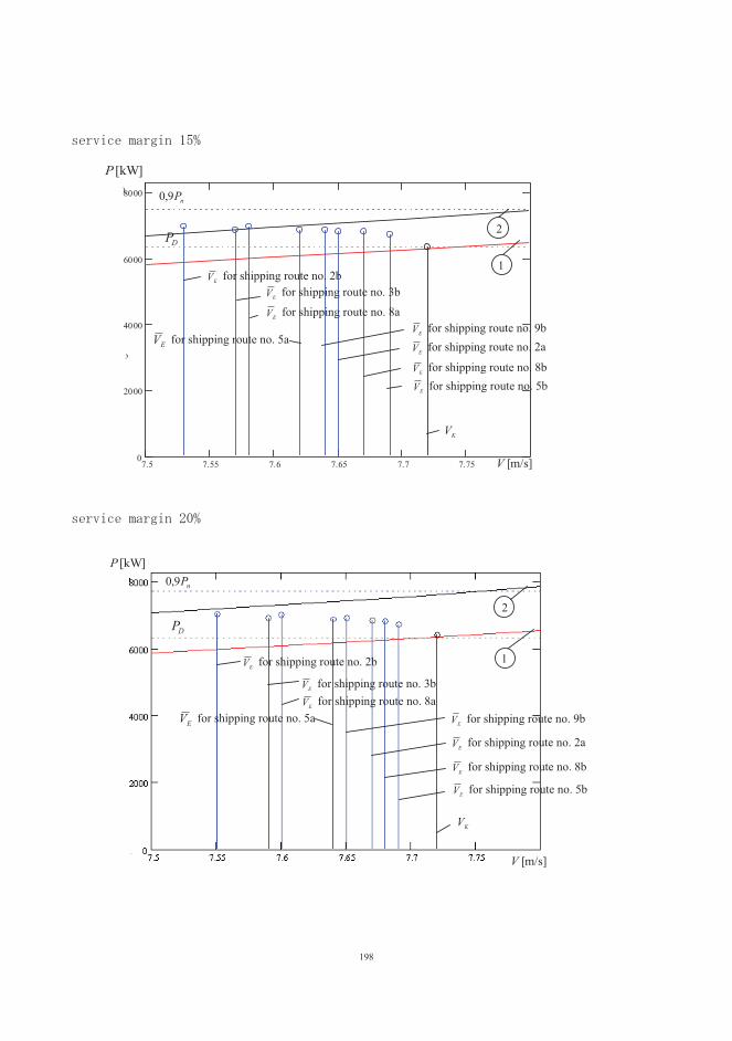
7.5 7.55 7.6 7.65 7.7 7.750
2000
4000
6000
80008300
1.538 103�
P D
P Dnom
P D15
P Dws
P Dtrwyb
P Dws1
7.87.5 V V pom5 V5 V ws5 V trwyb5 V pom5
nP9,0
[kW] P
[m/s] V
DP
KV
EV for shipping route no. 2bEV for shipping route no. 3b
EV for shipping route no. 8aEV for shipping route no. 9b
EV for shipping route no. 2a
EV for shipping route no. 8b
EV for shipping route no. 5a
EV for shipping route no. 5b
2
1
nP9,0
DP2
1
[kW] P
EV for shipping route no. 2b
EV for shipping route no. 3b
EV for shipping route no. 8a
EV for shipping route no. 5aEV for shipping route no. 9b
EV for shipping route no. 2a
EV for shipping route no. 8b
EV for shipping route no. 5b
[m/s] V
KV
198

7.5 7.55 7.6 7.65 7.7 7.750
2000
4000
6000
80008300
1.581 103�
P D
P Dnom
P D15
P Dws
P Dtrwyb
P Dws1
7.87.5 V V pom5 V5 V ws5 V trwyb5 V pom5
Fig. 6. Mean statistical working point of a screw propeller of K1 ship depending on a mean statistical long-term service speed V E on various sailing routes
� still-water propeller curve, � propeller curve containing the service margin SM = 15%, 20%, 25%,PD � power delivered to propeller cone at ship’s contractual speed in still water conditions,Nn � nominal power output of
propulsion engine,
EV � mean statistical long-term value of ship service speed on given shipping route,VK � contractual speed of ship
Table 1. Mean statistical of service parameters M2 ship for route 2b and 5b
Shipping route Route no. 2b Route no. 5bService margin 15% 20% 25% 15% 20% 25%Probability of maintaining the assumed speed V = 7,72 [m/s]
0,55 0,79 0,82 0,86 0,96 0,97
Mean statistical service speed EV [m/s]
7,53 7,55 7,58 7,68 7,69 7,70
Mean statistical propeller thrustT [kN]
752 785 790 741 752 753
Mean statistical propeller speed pn [1/s]
2,021 2,063 2,070 2,031 2,045 2,047
Mean statistical propeller efficiency 0� [-]
0,499 0,499 0,499 0,510 0,510 0,510
21
nP9,0
[kW] P
[m/s] V
DP
KV
1
2
EV for shipping route no. 2bEV for shipping route no. 3b
EV for shipping route no. 8a
EV for shipping route no. 5a
EV for shipping route no. 9b
EV for shipping route no. 2a
EV for shipping route no. 8b
EV for shipping route no. 5b
199

4. Mean statistical working point of propeller
Histograms of thrust, propeller speed and efficiency (Fig. 2 – 5) show, that working parameters of a propeller are largely dependent on weather conditions on a given sailing route. Mean statistical parameters of a propeller were calculated at different service margin values (SM = 15, 20 i 25%). In this case the main aim was to maintain the assumed speed without overloading the propelling engine. With such criterion in mind, it shows that the bigger the SM value the higher mean statistical service speed of a ship, while the exact value of SM did not have any major effect on propeller efficiency on a given sailing route (Table 1)
Bibliography
1. Szelangiewicz T., Żelazny K.: Calculation of Mean Long-Term Service Speed of Transport Ship, Part I: Resistance of Ship Sailing on Regular Shipping Route in Real Weather Conditions, Polish Maritime Research, No 4/2006
2. Szelangiewicz T., Żelazny K.: Calculation of Mean Long-Term Service Speed of Transport Ship, Part II: Service speed of ship sailing on regular shipping route in real weather conditions, Polish Maritime Research, No 1/2007
3. Szelangiewicz T., Żelazny K.: Calculation of Mean Long-Term Service Speed of Transport Ship, Part III: Wpływ linii żeglugowej i parametrów statku na jego prędkość eksploatacyjną, Polish Maritime Research, No 2/2007
4. Żelazny K.: Numerical prediction of mean long-term service speed of transport ship (in Polish). Doctoral thesis, Maritime Technology Faculty, Szczecin University of Technology, Szczecin 2005
5. Szelangiewicz T., Żelazny K.: Prediction of the influence of emergence of propeller on the propeller thrust and speed reduction during ship navigation on a given ocean route, Journal of Polish CIMAC, Gdańsk, 2010, Vol. 5, No. 2
The paper was published by financial supporting of West Pomeranian Province
200

INFLUENCE OF THE SERVICE MARGIN OF SERVICE PARAMETERS OF TRANSPORT SHIP PROPULSION SYSTEM
Part II
Screw propeller service parameters of transport ship sailing on a given shipping route
Tadeusz Szelangiewicz, Katarzyna Żelazny
Westpomeranian University of Technology in Szczecin, Faculty of Maritime Technology and Transport, Piastów 41, 71-065 Szczecin, Poland
tel. +48 91 449 41 26, fax: +48 91 449 46 95 e-mail: [email protected], [email protected]
Abstract
During ship sailing on a given shipping route in real weather conditions all propulsion system performance parameters of the ship change along with changes of instantaneous total resistance and speed of the ship. In this paper results of calculations are presented of distribution function and mean statistical values of screw propeller thrust, rotational speed and efficiency as well as propulsion engine power output and specific fuel oil consumption occurring on selected shipping routes at different service margin values. On this basis new guidelines for ship propulsion system design procedure are formulated.
Keywords: thrust, efficiency and rotational speed of screw propeller, long-term prediction, shipping route, design working point of screw propeller, service margin
5. Service parameters of propulsion engine operation
The service parameters of propulsion engine operation, calculated below for a ship sailing on a given shipping route at different service margin are as follows: � engine power output P� engine speed (number of engine revolutions per time unit) n� specific fuel oil consumption(SFOC), g, or hourly fuel oil consumption G.
The first two parameters (P, n) determine engine working point (if engine directly drives propeller without any reduction gear then n = np). During ship’s sailing on a given shipping route in changeable weather conditions the engine working point changes its location. By controlling fuel charge (consequently also number of revolutions) a new engine working point is searched with the use of the
201

criterion assumed below, so as to get it placed within engine layout area. Change of location of the engine working point makes fuel oil consumption changing: both the specific, g, and hourly one G.
6. Engine performance characteristics and load diagram
The propulsion engine load diagram consists of a few areas limited by appropriate characteristic lines. Working point of propulsion engine can be located in the areas but in some of them – only for a determined time of operation. The example load diagram of a Sulzer propulsion engine is shown together with depicted SFOC characteristics in Fig. 7.
Fig. 7. Load diagram of a propulsion engine [8]. Pn − rated torque, nn - nominal engine speed, A − continuous rating area (green); B − engine overload area
(red); C − sea trial rating area (blue); D − still-water optimum rating area (...); E − instantaneous rating area (yellow)
The particular areas are limited by engine performance characteristics of the following form:
mm nkP �� (2)
where: P - engine power output km - coefficient for a given characteristic line n - engine speed m - exponent depending on an engine type and producer; for SULZER RTA 52, RTA 62, RTA 72,
RTA 84 slow speed diesel engines:
[-] PnP
[-] nn
n
199
200
201
202
203204
205 g/kWh
AD
B
E
C
202

m = 0 - for nominal continuous rating or maximum continuous rating, m = 1 - for constant torque characteristics, m = 2.45 - for overload characteristics.
Particular characteristics and range of engine speed are determined depending on an engine type (producer).
In Fig. 7, on the engine load diagram the SFOC characteristics, g, are shown. They are provided by engine producer and valid for a given engine and determined conditions (a given air temperature etc). There are also more general characteristics published by engine producers in the form of relevant nomograms, e.g. [8], which make it possible to calculate the SFOC depending on an engine type (producers), its nominal parameters (power and speed), instantaneous engine load as well as ambient conditions (temperature of air and cooling water). The way of making use of the nomograms to calculate the SFOC of engines is given in [5]. Fuel consumption can be also determined on the basis of measurements carried out with the use of special instruments (flow meters, calibrated tanks) during propulsion engine operation [1].
7. Ship propulsion characteristics – propulsion system’s performance in changeable weather conditions
The ship propulsion characteristics are the following : curves of propulsion power, thrust, efficiency and torque at propeller’s cone, fuel consumption and ship speed available for a given ship resistance characteristic. The characteristics are usually presented on the propulsion engine load diagram in function of propeller (engine) speed or ship speed (then characteristic of constant number of revolutions is attached). The propulsion characteristics published in the subject-matter literature are usually elaborated on the basis of: O model test results of free propellers or behind-the-hull onesO results of measurements carried out on ship board [2, 7]O results of measurements carried out on ship board with simultaneous use of free-propeller
characteristics derived from model tests or numerically determined [3, 4, 5, 6]. For purposes of this work a numerical method for predicting the ship propulsion characteristics
was elaborated (for a designed ship appropriate model tests are not to be performed), in the following form: • T(V, n) - propeller thrust • Q(V, n) - propeller torque • η0(V, n) - propeller efficiency• PD(V, n) - power output at propeller’s cone• V(PD, n) - ship speed characteristic
where: V - ship speed n - engine speed (if the engine is of a slow speed then n = np, where np - propeller speed).
The above characteristics together with the criteria for selecting service parameters for a ship in a changeable weather conditions are shown in [10].
203

8. Results of calculations mean statistical parameters of engine for ship sailing on route
Results of the calculations for the selected ship and shipping route (engine and shipping route parameters were specified in [9]), are presented in the form of : O engine speed histogram and mean statistical value O engine power output histogram and mean statistical valueO specific fuel oil consumption (SFOC) distribution function and mean statistical valueO probability distribution function of long-term occurrence of given values of engine speed and
output (histogram of engine’s working point)O mean, long-term working point of propulsion engine.
In the figures the calculation results are presented – under the assumption that engine’s output reaches at most 0.9 Pn - for M2 [9] and the two very different shipping routes : 5b - “easy” one and 2b - „difficult” one - in the sense of occurrence of long-term weather parameters.
Ship: M2 - assumed service speed = 7,72 [m/s] SM=15% - probability of mantaining a given speed
VEPRoute no. 2b -
VEP = 0,55 Route no. 5b - VEP = 0,86
Engine speed histograms
0
0,1
0,2
0,3
0,4
0,5
0,6
0,7
0,8
0,9
1
0,34
2
0,72
2
0,79
7
0,87
2
0,94
7
1,02
2
1,09
7
1,17
2
1,24
7
1,32
3
1,39
8
1,47
3
1,54
8
1,62
3
1,69
8
1,77
3
1,84
8
1,92
3
1,99
9
2,07
4
Nominal engine speed nn = 2,030 [1/s]Mean engine speed n = 2,021 [1/s]
0
0,1
0,2
0,3
0,4
0,5
0,6
0,7
0,8
0,9
1
0,34
2
0,72
2
0,79
7
0,87
2
0,94
7
1,02
2
1,09
7
1,17
2
1,24
7
1,32
3
1,39
8
1,47
3
1,54
8
1,62
3
1,69
8
1,77
3
1,84
8
1,92
3
1,99
9
2,07
4
n[1/s]Mean engine speed n = 2,031 [1/s]
Power output histograms
0
0,2
0,4
0,6
0,8
1
388
954
1308
1661
2015
2369
2723
3077
3431
3785
4138
4492
4846
5200
5554
5908
6262
6615
6969
7323
Nominal power output nP = 7500 [kW]
Mean power output P = 6970 [kW]
0
0,2
0,4
0,6
0,8
1
388
954
1308
1661
2015
2369
2723
3077
3431
3785
4138
4492
4846
5200
5554
5908
6262
6615
6969
7323
N[kW]Mean power output P = 6724 [kW]
TnP
TPP
TnP
TPP
204

SM=20% Route no. 2b - VEP = 0,79 Route no. 5b - VEP = 0,96
Engine speed histograms
0
0,1
0,2
0,3
0,4
0,5
0,6
0,7
0,8
0,9
1
0,34
7
0,73
1
0,80
8
0,88
4
0,96
0
1,03
6
1,11
2
1,18
8
1,26
4
1,34
0
1,41
6
1,49
3
1,56
9
1,64
5
1,72
1
1,79
7
1,87
3
1,94
9
2,02
5
2,10
2
Nominal engine speed nn = 2,057 [1/s]Mean engine speed n = 2,063 [1/s]
0
0,1
0,2
0,3
0,4
0,5
0,6
0,7
0,8
0,9
1
0,34
7
0,73
1
0,80
8
0,88
4
0,96
0
1,03
6
1,11
2
1,18
8
1,26
4
1,34
0
1,41
6
1,49
3
1,56
9
1,64
5
1,72
1
1,79
7
1,87
3
1,94
9
2,02
5
2,10
2
n[1/s]Mean engine speed n = 2,045 [1/s]
Power output histograms
0
0,2
0,4
0,6
0,8
1
401
986
1351
1717
2082
2448
2814
3179
3545
3911
4276
4642
5008
5373
5739
6105
6470
6836
7202
7567
Nominal power output nP = 7750 [kW]
Mean power output P = 7044 [kW]
0
0,2
0,4
0,6
0,8
1
401
986
1351
1717
2082
2448
2814
3179
3545
3911
4276
4642
5008
5373
5739
6105
6470
6836
7202
7567
N[kW]Mean power output P = 6740 [kW]
SM=25% Route no. 2b - VEP = 0,82 Route no. 5b -
VEP = 0,97 Engine speed histograms
0
0,1
0,2
0,3
0,4
0,5
0,6
0,7
0,8
0,9
1
0,35
2
0,74
4
0,82
1
0,89
8
0,97
6
1,05
3
1,13
1
1,20
8
1,28
5
1,36
3
1,44
0
1,51
8
1,59
5
1,67
2
1,75
0
1,82
7
1,90
4
1,98
2
2,05
9
2,13
7
Nominal engine speed nn = 2,092 [1/s]Mean engine speed n = 2,070 [1/s]
0
0,1
0,2
0,3
0,4
0,5
0,6
0,7
0,8
0,9
1
0,35
2
0,74
4
0,82
1
0,89
8
0,97
6
1,05
3
1,13
1
1,20
8
1,28
5
1,36
3
1,44
0
1,51
8
1,59
5
1,67
2
1,75
0
1,82
7
1,90
4
1,98
2
2,05
9
2,13
7
n[1/s]Mean engine speed n = 2,047 [1/s]
Power output histograms
0
0,2
0,4
0,6
0,8
1
418
1026
1407
1788
2168
2549
2930
3311
3691
4072
4453
4834
5214
5595
5976
6357
6737
7118
7499
7880
Nominal power output nP = 8070 [kW]
Mean power output P = 7123 [kW]
0
0,2
0,4
0,6
0,8
1
418
1026
1407
1788
2168
2549
2930
3311
3691
4072
4453
4834
5214
5595
5976
6357
6737
7118
7499
7880
[kW]Mean power output P = 6756 [kW]
TnP
TnP
TPP
Fig. 8. Histograms and mean statistical values of speed and output of engine at different service margin values for routes no. 2b and 5b
TPP
TnP
TPP
TnP
TPP
205

Ship: M2 - assumed service speed = 7,72 [m/s] SM=15% - mean fuel oil consumption in still water g = 199,00 g/kWh
Route 2b Route 5b
0
0,1
0,2
0,3
0,4
0,5
0,6
0,7
0,8
0,9
1
198
199
200
201
202
203
204
205
206
207
Mean fuel oil consumption = 199,01 g/kWh
0
0,1
0,2
0,3
0,4
0,5
0,6
0,7
0,8
0,9
1
198
199
200
201
202
203
204
205
206
207
g[g/kWh]
Mean fuel oil consumption = 199,00 g/kWh
SM=20%
Route 2b Route 5b
0
0,1
0,2
0,3
0,4
0,5
0,6
0,7
0,8
0,9
1
198
199
200
201
202
203
204
205
206
207
Mean fuel oil consumption = 199,01 g/kWh
0
0,1
0,2
0,3
0,4
0,5
0,6
0,7
0,8
0,9
1
198
199
200
201
202
203
204
205
206
207
g[g/kWh]
Mean fuel oil consumption = 199,00 g/kWh
SM=25%
Route 2b Route 5b
0
0,1
0,2
0,3
0,4
0,5
0,6
0,7
0,8
0,9
1
198
199
200
201
202
203
204
205
206
207
Mean fuel oil consumption = 199,13 g/kWh
0
0,1
0,2
0,3
0,4
0,5
0,6
0,7
0,8
0,9
1
198
199
200
201
202
203
204
205
206
207
g[g/kWh]
Mean fuel oil consumption = 199,00 g/kWh
TgP
TgP
TgP
Fig 9. Histograms and mean statistical values of fuel oil consumption at different service margin values for routes no. 2b and 5b
TgP
TgP
TgP
206

Fig 10. Mean, long-term working point of engine at different service margin values for routes no. 2b and 5b
207

Route 2b
0,80
0,85
0,90
0,95
1,00
1,05
1,10
0,90 0,95 1,00 1,05 1,10
Route 5b
0,80
0,85
0,90
0,95
1,00
1,05
1,10
0,90 0,95 1,00 1,05 1,10
Fig. 11. Influence of the service margin of mean long-term working point of engine for routes no. 2b and 5b
SM=15% SM=20%SM=25%
SM=15%SM=20%
SM=25%
Rel
ativ
e en
gine
pow
er o
utpu
t [%
CM
CR
]
Relative engine speed [% CMCR]
Relative engine speed [% CMCR]Rel
ativ
e en
gine
pow
er o
utpu
t [%
CM
CR
]
208

Final conclusions
o Conclusion results from the calculations of mean statistical service parameters of screw propeller were presented in [10]. Results of the calculations of the mean statistical parameters of propulsion engine operation c (engine, speed, output and specific fuel oil consumption – SFOC) in the from of histograms are very similar to those of screw propeller as the engine in question directly drives the propeller and the calculated power output is used only for propelling the ship (as no other power consumers were taken into consideration, e.g. shaft generators)
o The calculations of SFOC were performed for approximate characteristics under the assumption that the engine is new, air and cooling water parameters are standard and ship’s hull and screw propeller are clean (unfouled). Therefore the calculation results should be assessed rather qualitatively but not quantitatively.
o The obtained histograms and mean statistical parameters depend not only on weather conditions on a given shipping route but also on a assumed criterion of propulsion control; the presented calculations were performed for the criterion of maintaining the ship speed constant (Variant “b”, Fig. 11) and if it is not possible – for a maximum available speed at the engine power output of 0,9
nP at the most. The assumed criteria of ship propulsion (engine) control highly influence service parameters of propulsion system. This can be observed in the case of the SFOC distribution as well as occurrence probability of a given working point of engine on a given shipping route.
o The condition of maintaining the assumed ship speed may results in a somewhat greater SFOC value on a shipping route where statistically more favourable weather conditions occur than on those of more harsh weather conditions. Hence not only weather conditions occurring on a shipping route are decisive of fuel consumption level. Therefore to obtain a possibly low SFOC level the propulsion control should be optimized by using various criteria (Fig. 11) depending on a given situation. In real conditions also ship course can be changed that consequently is equivalent to shipping route optimization.
o The elaborated computer software makes it possible to choose different control criteria of ship propulsion and optimize booth its service parameters and entire shipping route.
o Calculations of probability of occurrence of propulsion engine working point (Fig. 10, 11 as for scheduling overhauls).
o The influence of the SM values on mean statistical service parameters of a ship is depends mainly on the assumed criterion of ship propulsion. In this article it is assumed, that the assumed speed of a ship with be maintained. As results the higher the SM value, the higher also mean statistical service speed of a ship and therefore the higher probability of maintaining the assumed service speed of a ship (Table 1). All the remaining parameters: thrust, propeller efficiency, power speed engine and average working point of the propulsion engine sent from the adopted criterion of maintaining the assumed service speed.
209

Bibliography
1. Balcerski A.: Modele probabilistyczne w teorii projektowania i eksploatacji spalinowych siłowni okrętowych, Fundacja Promocji Przemysłu Okrętowego i Gospodarki Morskiej, Gdańsk 2007
2. Beukelman W., Buitenhek M.: Full scale measurements and predicted seakeeping performance of the containership “Atlantic Crown” , International Shipbuilding Progress, Vol. 21, No. 243, 1974, pp. 325�351
3. Chachulski K.: Energetyczne problemy eksploatacji napędów okrętowych, Wydawnictwo Morskie, Gdańsk 1991
4. Chachulski K.: Kontrola stanu obciążenia silnika napędowego i jego zużycia paliwa w każdych warunkach pływania, XIV International Symposium of Ship Power Plants, Szczecin, 1992, str. 9 �23
5. Chachulski K.: Metody i algorytmy rozwiązywania problemów eksploatacyjno-ruchowych okrętowych układów napędowych, Wyższa Szkoła Morska, Szczecin, 1992
6. Chachulski K.: Podstawy napędu okrętowego, Wydawnictwo Morskie, Gdańsk 19887. Ferdinande V., De Lembre R.: Service - performance and seakeeping trials on a car-ferry,
International Shipbuilding Progress, Vol. 17, No. 196, 1970, pp. 361�3948. General Technical Data for Marine Diesel Engines, SULZER, 1986 9. Szelangiewicz T., Żelazny K.: Calculation of the mean long-term service speed of transport ship Part III –Influence of shipping route and ship parameters on its service speed, Polish Maritime
Research, No 2/2007, pp. 27 � 3210. Szelangiewicz T., Żelazny K.: Mean long-term service parameters of transport ship propulsion
system, Part. II – Propulsion engine service parameters of transport ship sailing on a given shipping route, Polish Maritime Research, No. 4(54), Vol. 14, 2007, pp. 47 � 52
The paper was published by financial supporting of West Pomeranian Province
210

THE EFFECTIVENESS OF RIGID ROTOR’S BALANCE WITH RESONANT EXTORTION OF THE SYSTEM WITH SMALL DAMPING
Janusz Zachwieja, Henryk Holka
University of Technology and Life Sciences in Bydgoszcz ul. S. Kaliskiego 7, 85-789 Bydgoszcz, Polska
email: [email protected]
Abstract
The thesis refers to the previous researches of the authors of the dynamics of rigid rotor placed on favourable ground. Such systems are characterized by usually low frequency of normal mode vibrations which causes real danger that they can work in the resonant region or cross this region every time during acceleration or start. The amplitude of rotor's vibrations with small internal damping reaches then high values. The factor of damping for the system with small mass may be defined on the basis of the character of its response to pulse extortion. The way how to determine the value of rotor's damping useful for the numerical analysis of its vibration was presented. The thesis presents also the results of the researches of the effectiveness of disk balance with circum-resonant speed in the situations when only unbalanced force affects the rotor and when vibrations of the foundation are caused by the external resonant induction.
Keywords: rigid rotor balancing natural frequencies vibrations
1. Introduction The foundations of the machines are sometimes characterized by relatively high susceptibility and small damping because of which the amplitude of their vibrations may reach high values even with small extortion [1]. The supporting construction of the separator presented in the Fig. 1.1 is an example of incorrect approach to the way of designing depending on taking into account only the aspect of endurance and excluding the conclusions drawn from the analysis of normal mode vibrations of the construction [2]. Low rigidity of the foundation of bicarbonate separator (Fig.1.2) is the consequence of thoughtful action and results from the necessity of providing the machine with the accurate vibration isolation [3].
If the frequency of normal mode vibrations of the foundation is low there is a greater danger that lying on it rotor machine will incur vibrations of resonant character during work as well as during acceleration or start. The frequencies of extortions affecting the foundation result from speed motor drive (25Hz or 50 Hz) if the unbalanced rotor is directly connected to the motor or they may be completely arbitrary if there is a gear in the motor drive system. In numerous situations several machines of one processing line are placed on the same foundation, constituting a disturbance for each other (Fig. 1.3).
211

Fig.1.1. The view of the separator’s springer construction
Fig. 1.2. The manner of bicarbonate centrifuge founding
Fig. 1.3. A row of ventilators placed on a common foundation
Resonant qualities of the system and its damping are features between which there is a great co-dependence. The bigger damping, the less clear response of the resonant system. Resonant vibrations of the construction, besides the case of its vibratory stress relief [4,5], are harmful and may lead to the catastrophe caused by big deformations of its elements and subsidence of the foundation which supports it [6].
Vibrations are the main cause of reducing vivacity of machine's elements, especially bearings. Usually the rotating parts are not allowed to work in their resonant region. The deviation from the rule are operating conditions of turbine's rotor which frequency of normal mode vibrations is only slightly lower than rotational frequency. It is the feature of flexible rotors owing to which they are subject to self-aligning after crossing critical speed. Anisotropy of rotor's rigidity causes growth of the number of resonant frequencies between which there are regions of backward precession [7]. Itmeans that the rotor is exposed to be in the regions of prohibited speed several times.
Rotor's balance with the circum-resonant speed encounters numerous difficulties mainly because of instability of the amplitude as well as its angles of phase vibration. Its effectiveness in most cases is not satisfactory and it is necessary to include in the method of impact factors special averaging algorithms in order to improve the accuracy of calculations when determining correlation masses [8,9].
2. The analysis of impact of damping on rotor's vibration in the region of resonance occurrence
When modelling vibrations of rigid rotor it is convenient to treat all elements of the system as non-deformable bodies with the exception of elements which susceptibility has an impact on the character of its functioning. Coupling and vibroisolators belong to the group. In the case of the later their rigidity is usually known although the values given by the producer slightly vary from the once obtained during verifying researches. The value of damping is unknown. If the rotor is placed directly on the foundation, the susceptibility of the foundation is the unknown which should be defined. The possible procedure is exemplified by the rotor presented in the Fig. 2.1. It has 2 disks which are the correlation surfaces during balance. The drive from the motor with the adjustable rotational frequency is transferred to the rotor by rigid coupling of Rotex type with polyurethane footbed with hardness of 92°Sh. On the frame, together with the rotor there is an inductor with forced frequency adjustable by frequency converter. The total mass of the stand is ~120 kg. The frame is placed on the favourable ground.
212

Fig. 2.1. Test stand: 1. two-disk rotor, 2. motor, 3. coupling, 4. indicator, 5. frame, 6. favourable ground
Fig. 2.2. Numerical model of the test stand
The resonant characteristic of the rotor was determined in two ways: by pulse induction and by using short-term Fourier transform for the analysis of time course of vibrations during the start of the inductor. According to the expectations, the basic resonant frequencies of rotor's vibrations are low and amount to: horizontal surface - ~6Hz, vertical surface -~11 Hz (Fig. 2.3.).
68H
z
11H
z
83H
z
0
0,01
0,02
0,03
0,04
0,05
0,06
0,07
0,08
0,09
0,1
0 50 100Hz
mm
/s
a)
27H
z
17H
z
83H
z
48H
z
6Hz
0
0,01
0,02
0,03
0,04
0,05
0,06
0,07
0,08
0,09
0,1
0 50 100Hz
mm
/s
b)Fig. 2.3. Resonant characteristics of rotor’s vibrations determined during the start of the inductor: a) vertical
surface, b) horizontal surface
To describe the qualities of the rotor the so-called flat model was used, which equations of movement can be presented by coordinates complex as [10]
� �tmxkxcxm xx DD� cos2��� ���� and � �tmykycym yy DD� sin2��� ��� (2.1)
Assuming signs iyxz �� , iyxz �� and multiplying by i The second equation and adding to both sides of equation we receive
)exp(2 timzkzkzczczm dsds DD������ ���� (2.2)
where2
yxs
ccc
�� and
2yx
dcc
c�
� , as well as2
yxs
kkk
�� and
2yx
dkk
k�
� , moreover: m – rotor’s
mass, cx, cy – damping factor, kx, ky – rigidity, ε�� - vector module of the location of the rotor’scentre of gravity against the axis of rotation, D - angular velocity.
The rigidity of the rotor's foundation may be determined if we know its mass and resonant frequencies. For example, the model presented in the Fig. 2.2 has, with the same mass as the rotor, similar resonant frequencies if the rigidities of the bearing are adequately 100N/mm in horizontal direction and 300N/mm in vertical direction. Corresponding to them normal forms are presented in the Fig. 2.4. The amplitude-frequency characteristic in the range of frequency (0-20 Hz) confirms the result received earlier by the use of inductor (Fig. 2.5b).
0 6 12 18 24 30
30
24
18
12
6
0
0.02
0.018
0.016
0.014
0.012
0.010
0.008
0.006
0.004
0.002
0
m/s2Hz
0 6 12 18 24 30
30
24
18
12
6
0
0.02
0.018
0.016
0.014
0.012
0.010
0.008
0.006
0.004
0.002
0
m/s2Hz
11Hz
17Hz
6Hz
1 23 4
65
K1
213

6.3Hz 11.3Hz 16.5Hz
Fig. 2.4. The forms of norma mode vibrations – equilibrium position marked yellow
The bigger problem is to estimate the value of damping. The possible way to define it is to determine the logarithmic decrement. The system with one degree of freedom which response to the implemented extortion is described by harmonic function, there are dependencies between the damping factor, mass and logarithmic decrement.
mch
2� and
2ln
1
ThAAi
i ����
!!"
#�
�9
(2.3)
Converting the compounds (2-3) we receive the dependencies of damping factor in the form of
Tmc 94
�(2.4)
Here: 9 - logarithmic decrement, T – vibrations period.
-5
-4
-3
-2
-1
0
1
2
3
4
5
1,5 2 2,5s
mm
/s
a)
-0,5
-0,4
-0,3
-0,2
-0,1
0
0,1
0,2
0,3
0,4
0,5
0 5 10 15 20
Hz
mm
/s
b)Fig.2.5. The response of the system to pulse induction: a) time course, b) characteristic A-C
The analysis of the rotor's response to the pulse induction defines logarithmic decrement with the precision sufficient to the accurate estimation of the value of factor c. For example, the response of the system to pulse induction in vertical direction is shown in Fig. 2.5a.
-5
-4
-3
-2
-1
0
1
2
3
4
5
1,5 2 2,5
s
mm
/s
-0,5
-0,4
-0,3
-0,2
-0,1
0
0,1
0,2
0,3
0,4
0,5
0 5 10 15 20
Hz
mm
/s
-5
-4
-3
-2
-1
0
1
2
3
4
5
1,5 2 2,5
s
mm
/s
-0,5
-0,4
-0,3
-0,2
-0,1
0
0,1
0,2
0,3
0,4
0,5
0 5 10 15 20
Hz
mm
/s
Fig.2.6. The figure of the system’s response In horizontal direction after Hilbert-Huang transform
Fig. 2.7. Numerical solution of the system’s response inhorizontal direction for the approved model
6Hz 11
Hz
17H
z
6Hz
6Hz
17H
z
214

We will obtain the character of rotor's vibrations in natural frequencies after putting on the signal the narrow-band filter. This function is served well by Hilbert-Huang transform. Fig. 2.6 and 2.8 present the effect of the filtration of the signal presented in the Fig. 2.5 to obtain a clear course of the response of the system in frequencies of 6 Hz and 11 Hz. The use of the filter allows the analysis of the character of rotor's vibrations in orthogonal directions by the induction only in the direction of its smaller rigidity. It is crucial in the case of anisotropic susceptibility of bearing with great asymmetry requiring the use in the direction of bigger rigidity greater force to obtain a clear response of the system to the induction. Comparing the shape of the functions crucial (IMF - Intrinsic Mode Functions). for resonant frequencies with time course of the response obtained from numerical solution of the model's vibrations, a great similarity for damping factor 1 Ns/mm in horizontal direction (Fig. 2.6s and 2.7a) and for damping factor 2 Ns/mm in vertical direction (Fig. 2.8a and 2.9a) can be observed.
-5
-4
-3
-2
-1
0
1
2
3
4
5
1,5 2 2,5
s
mm
/s
a)
-0,5
-0,4
-0,3
-0,2
-0,1
0
0,1
0,2
0,3
0,4
0,5
0 5 10 15 20
Hz
mm
/s
b)
-5
-4
-3
-2
-1
0
1
2
3
4
5
1,5 2,5
s
mm
/s
a)
-0,5
-0,4
-0,3
-0,2
-0,1
0
0,1
0,2
0,3
0,4
0,5
0 5 10 15 20
Hz
mm
/s
b)Fig. 2.8. The figure of the system’s response in vertical
direction after Hilbert-Huang transform Fig. 2.9. Numerical solution of the system’s response in
horizontal direction for the approved model
The final verification of the accurate choice of physical parameters of the model is the accordance of the shape of time course of rotor's vibrations speed during a run-up with numerical solution for an analogous case (Fig. 2.10a – 2.10b). As we can see such big damping of the system causes crossing the resonant region by the rotor during a run-up in a gentle way.
Having the proper model available, we can conduct the stimulation showing the impact of the damping on the rotor's behaviour when it is crossing the resonance for the equal damping values. The similar analysis should proceed the choice of vibro-isolators every time, especially if they have damping qualities (the so-called viscous damper).
-8
-6
-4
-2
0
2
4
6
8
0 10 20 30
mm
/s
s
a)
-8
-6
-4
-2
0
2
4
6
8
0 10 20 30
s
mm
/s
b)
-8
-6
-4
-2
0
2
4
6
8
0 10 20 30
s
mm
/s
c)Fig. 2.10. Time courses of vibrations of: a) rotor, b) its model with similar rigidity and damping, c) rotor’s model with
small damping
Fig. 2.10c shows the anticipated time course of rotor's vibrations with unbalanced disk during acceleration to rotational frequency of 25Hz when the damping factor equals 0,1 Ns/mm. Its ten
11H
z
11H
z
215

times smaller value than the actual one does not have a significant impact on the level of the forced vibrations, but the amplitudes of vibrations in the resonant region increase significantly.
3. Rotor’s balance outsider the resonant region In order to examine the impact of induction of natural frequency on the course and obtained
quality, the rotor was balanced in two phases. First, with the rotational frequency of 15 Hz without additional extortion affecting the rotor, and then with additional induction of circum-resonant frequency of 10,5Hz. Unbalancing of the rotor was the result of attaching to the disk K1 mass mn=(20g<900). The amplitude-frequency characteristics presented in Fig. 3.1 show this dynamic condition.
15H
z
0
2,5
5
7,5
10
12,5
15
0 10 20 30 40 50Hz
mm
/s
a)
15H
z
0
2,5
5
7,5
10
12,5
15
0 10 20 30 40 50Hz
mm
/s
b)15
Hz
0
2,5
5
7,5
10
12,5
15
0 10 20 30 40 50Hz
mm
/s
c)
15H
z
0
2,5
5
7,5
10
12,5
15
0 10 20 30 40 50Hz
mm
/s
d)Fig. 3.1. The amplitude-frequency characteristics of rotor’s vibrations speed with rotational frequency of 15 Hz and
unbalance of 20g mass attached to the disk K1.
The result achieved by balancing the rotor with the optimisation of the value of the amplitude of both bearings movement is presented by holospectra 1x (Fig. 3.2-3.3). The optimisation algorithm P(1,2,3,4) used for the correlation K(1) using the disk to which the mass mn is attached, determined the correcting mass mk=(22.3g<2600). The achieved result is correct and the slight difference does not result from calculation error, but from the existing initial unbalance of the disk (Fig. 3.2).
Fig. 3.2. The comparison of the rotor’s movement inBering surfaces a) initial sate, b) after the balance,
without additional extortion of foundation vibrations
Fig. 3.3. The comparison of the rotor’s movement in bearing surfaces a) initial state, b) after the balance, without additional extortion of frame vibrations of
frequency of 10.5Hz
The repeated process of balancing with the same frequency and additional induction resulted in what is presented in Fig. 3.3. The picture of the dynamic condition of the rotor before the balance is presented in Fig. 3.4 in the form of the amplitude-frequency characteristic of vibrations speed.
600
400
200
050
0
-500
50
mm
Pm Pm
600
400
200
050
0
-500
50
mm
Pm Pm
600
400
200
050
0
-500
50
mm
Pm Pm
600
400
200
050
0
-500
50
mm
Pm Pm
216

10,5
Hz
15H
z
0
2,5
5
7,5
10
12,5
15
0 10 20 30 40 50Hz
mm
/s
a)10
,5H
z
15H
z
0
2,5
5
7,5
10
12,5
15
0 10 20 30 40 50Hzm
m/s
b)
10,5
Hz
15H
z
0
2,5
5
7,5
10
12,5
15
0 10 20 30 40 50Hz
mm
/s
c)
10,5
Hz
15H
z
0
2,5
5
7,5
10
12,5
15
0 10 20 30 40 50Hz
mm
/s
d)Fig. 3.4. The amplitude-frequency characteristics of vibrations speed of the rotor with the rotational frequency of 15
Hz and the unbalance of 20g mass attached to The disk K1 induction with frequency of 10.5 Hz
Circum-resonant induction caused the deterioration of the achieved balanced quality. It can be seen especially with reference to the vibrations of the bearing placed further from the correlation surface.
4. Balance in the resonant region
The essence of the resonant vibrations is that even small extortion reflects in the response of the system with high amplitude values. When balancing the rotor we are usually not aware that its rotational frequency is close to natural frequency and the unbalance has secondary meaning. We expect to achieve the effect in the form of multiple decrease of the level of vibrations. It causes the situation in which we manage to limit this level, but further action proves to be ineffective. The calculated correcting mass causes another balancing of the rotor so that another one improves its dynamic condition.
Coaxial rotor with significant static unbalance can be balanced to a certain extent in the resonant region. To determine it to the disk K1 of the rotor presented in Fig. 2.1 mn=(20g<900)mass was attached. The achieved balance quality may be estimated comparing 1x holospectra of the rotor presented in Fig. 4.1-4.2 adequately for the circum-resonant frequencies 10,5 Hz and 6 Hz. Although the rotor's balance took place in the region of forced vibrations along with normal mode vibrations, two- and four-fold decrease of their level was achieved. It is not the satisfactory result if we compare it to the effect achieved during the balance of the rotor outside the resonant region.
a) b) c) d)
Fig. 4.1. The rotor’s holospectrum before and after the balance with the frequency of 10.5Hz
Fig. 4.2. The rotor’s holospectrum before and after the balance with The frequency of 6Hz
The analysis of the effectiveness of the balance in the resonant region of the rotor with the unbalance torque attaching to both disks the masses mn1=(10g<900) and mn2=(10g<2700) was conducted. They have identical values, however their peripheral location on the disk of the rotor vary by � angle. The extortion caused by such load during the rotor's rotation comes down to double force action. The balance was conducted with frequencies of 6 Hz, 8 Hz, 11 Hz and 15 Hz
600
400
200
0-200
0
-2000
200
mm
Pm Pm
600
400
200
0-200
0
-2000
200
mm
Pm Pm
600
400
200
0-100
0
-1000
100
mm
Pm Pm
600
400
200
0-100
0
-1000
100
mm
Pm Pm
217

so in the resonant regions, but also between them – in the conditions of backward precession, as well as the above second resonant frequency. Fig. 4.3-4.6 present the results.
Fig. 4.3. The rotor’s condition with the unbalance torque before and after the balance with 6Hz frequency
Fig. 4.4. The rotor’s condition with the unbalance torque before and after the balance with 8 Hz frequency
Fig. 4.5. The rotor’s condition with the unbalance torque before and after the balance with 11 Hz frequency
Fig. 4.6. The rotor’s condition with the unbalance torque before and after the balance with 15 Hz frequency
The result of the experiment is extremely interesting because of the fact that the clear decrease of the rotor's vibrations with the unbalance torque was achieved with critical velocity.
5. The balance of the rotor in the resonant region with the natural frequency induction An interesting case was observed during the rotor's balance with circum-resonant frequency of
10,5 Hz. The system was additionally inducted with synchronous frequency. To the disk K1 20g mass constituting its initial unbalance was attached.
c)
Fig.5.1. Holospectrum of the rotor’s vibrations with frequency of 10,5 Hz a) initial state, b) after the balance, c) after switching off the inductor
The fact that the rotor's balance was conducted with the resonant frequency did not disrupt its course, but it is hard to recognize the achieved effect as satisfactory. After the induction stopped the amplitudes of vibrations in the direction of resonance occurrence increased. The occurrence of
1000800600400200
0500
-500
50
mm
Pm Pm
1000800600400200
0500
-500
50
mm
Pm Pm
1000800600400200
0500
-500
50
mm
Pm Pm
1000800600400200
0500
-500
50
mm
Pm Pm
1000800600400200
0500
-500
50
mm
Pm Pm
1000800600400200
0500
-500
50
mm
Pm Pm
1000800600400200
0500
-500
50
mm
Pm Pm
1000800600400200
0500
-500
50
mm
Pm Pm
600
400
200
0-100
0
-100
0100
mm
Pm Pm
600
400
200
0-100
0
-100
0100
mm
Pm Pm
600
400
200
0-100
0
-100
0100
mm
Pm Pm
218

such effect means that the algorithm of the method of impact factors determines correlative masses based on the actual character of the rotor's vibrations. Its change may sometimes cause unexpected results.
6. Conclusions
The construction of the correct numerical model of the rotor requires the knowledge of its basic features such as mass, rigidity and damping. The rigid rotor may be treated as a compound system composed of non-deformable bodies because of the fact that the susceptibility of the rotor's shaft and disk is definitely smaller than in the case of the shoring. It definitely limits the number of freedom degrees and modelling process becomes relatively simple. The main problem still is the determination of its physical qualities such as rigidity and damping. It can be solved thanks to the knowledge of resonant characteristic of the actual system determined on the basis of pulse extortion. Knowing the rotor's mass and frequency of normal mode vibrations it is easy to estimate the rigidity occurring in the system and by determining the logarithmic decrement we receive approximate values of damping factors. This method can be used to examine the qualities of rotors with small mass and rigidity. Choosing the type of vibro-isolators it is necessary to remember that their damping qualities allow to reduce the amplitudes of the rotor's vibrations mainly with the natural frequency. The effect in the form of limiting the level of forced vibrations is not significant. The balance of the rigid rotor in the resonant region causes the fact that the achieved quality is not satisfactory. External extortion with resonant frequency reduces the effectiveness of the balance even more.
References
[1] Holka H., Effect of support structure receptance on mechanism operation. Developments in Machinery Design and Control 1, 41-49. 2005.
[2] Zachwieja J., Gołębiowska I., Damping of structures free vibrations based on the example of steel structure of separator’s foundation. Developments in Machinery Design and Control –Nowogród. 2008.
[3] Zachwieja J., Peszyński K., Vibroisolators application for damping vibtations in industrial fans. National Conference with International Participations – Engineering Mechanics Svratka Czech Republic. 2008.
[4] Zachwieja J., Diagnozowanie procesu odprężania wibracyjnego konstrukcji stalowych w celu doboru optymalnych parametrów technologicznych, Elementy diagnostyki maszyn roboczych i pojazdów, 283-294. 2009.
[5] Holka H., Nieckarz M., Usuwanie naprężeń spawalniczych w stalowych konstrukcjach metodami wibracyjnymi. Postępy w sterowaniu i konstrukcji – Bydgoszcz 2001.
[6] Zachwieja J., Numerical modelling of vibrations of machine foundations with percussive characteristics of work. Developments in Machinery Design and Control 5, 83-96. 2007.
[7] Muszyńska A., Rotordynamics. John Wiley & Sons Inc. 2005. [8] Kang Y., Liu C.P., Sheen G., A modified influence coefficient method for balancing
unsymmetrical rotor-bearing systems. Journal of Sound and Vibration 194(2), 199-218. 1996.[9] Lees A. W., Friswell M. I., The evaluation of rotor unbalance in flexibly mounted machines.
Journal of Sound and Vibration 208, 671-683. 1997. [10] Genta G., Whirling of unsymmetrical rotors: A finite element approach based on complex
coordinates. Journal of Sound and Vibrations 124(1), 27-53. 1988.
219

220