journal of membrane science & researcha system exhibiting simple permeation behaviour, this flux...

K E Y W O R D S

H I G H L I G H T S

A B S T R A C T

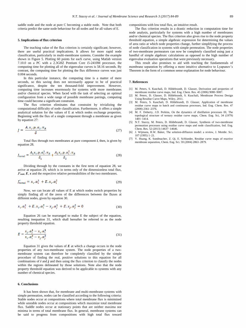
G R A P H I C A L A B S T R A C T

84

Research Paper

Received 2016-04-14Revised 2016-09-15Accepted 2016-09-17Available online 2016-09-17

MembranesSeparationMulti-membranePermeation

• It is shown that MRCM nodes can be classified using total membrane flux • Node property threshold equation is derived for rapidly selecting membrane area ratio• An intuitive understanding of membrane residue curve map topography is developed

Journal of Membrane Science and Research 3 (2017) 84-89

Shortcut Node Classification for Membrane Residue Curve Maps

1 University of Witwatersrand, Johannesburg, South Africa2 University of South Africa, Johannesburg, South Africa

Neil Thomas Stacey1,*, Mark Peters2, Diane Hildebrandt2, David Glasser2

A R T I C L E I N F O

© 2017 MPRL. All rights reserved.

* Corresponding author at: Phone: +27 11 670 8990; fax: +27 011 917 3048E-mail address: [email protected] (N.T. Stacey)

DOI: 10.22079/jmsr.2016.21846

1. Introduction

The vast majority of chemical processes require separation at some stage, be it in the preparation of suitable chemical feedstocks or the purifica-tion of reaction products. While distillation remains the most widely-used of separation processes alternatives have become increasingly popular, includ-ing absorption, solvent extraction and membrane permeation. Membrane permeation in particular has recently seen rapid development as a separation method.

Membrane permeators achieve separation by exposing a high-pressure fluid mixture to a membrane, through which components in the mixture per-meate at different rates, resulting in composition changes in both the residual fluid phase, called the retentate, and the stream of permeated material, called the permeate.

Peters et al. [1-3] developed Membrane Residue Curve Maps (MRCMs) as a tool for graphically tracking these composition changes, where curves are plotted by integrating the residue curve equation:

(1)

where x is the retentate composition expressed as a vector of component frac-tions and y is the composition of permeating material which is a function of x in accordance with the permeation modelling. τ is a dimensionless ratio, given by dividing the amount of material that has permeated to the amount that was initially present. In other words, at the commencement of permeation

http://dx.doi.org/10.22079/jmsr.2016.21846

Journal of Membrane Science & Research

journal homepage: www.msrjournal.com

Node classification within Membrane Residue Curves (M-RCMs) currently hinges on Lyapunov’s Theorem and therefore the computation of mathematically complex eigenvalues. This paper presents an alternative criterion for the classification of nodes within M-RCMs based on the total membrane flux at node compositions. This paper demonstrates that for a system exhibiting simple permeation behaviour, this flux criterion is mathematically identical to Lyapunov’s theorem for all possible values of relative permeability. This means that in membrane permeation systems with simple permeation, the stationary point with maximum flux is an unstable node while the stationary with minimum flux is a stable node and stationary points with intermediate fluxes are saddle points. This proof is also extended to two-membrane systems with simple permeation behaviour, resulting in a system of equations useful for finding membrane area ratios with desired node properties. It is also shown that the flux criterion does not hold for systems exhibiting complex permeation.

N.T. Stacey et al. / Journal of Membrane Science and Research 3 (2017) 84-89

τ=0 and when all material have completely permeated, then τ=1. M-RCMs

behave similarly to RCMs and for a full account of the development and

application of RCMs in a general sense, the reader is referred to Doherty [4]. M-RCMs have proven to be a useful design tool for rapid evaluation of

the separation behaviour of a particular membrane. They have also proven to

be a useful teaching tool, just like distillation RCMs before them, enabling the same intuitive understanding of the fundamentals of membrane separation.

Stacey et al. [5] extended the residue curve equation to include any

number of material streams being removed from the initial charge with the generalised equation:

(2)

In the specific case of a two-membrane permeator, this equation takes the

following form:

(3)

where the m in the superscripts indicates that the stream in question is exiting

via membrane permeation and the accompanying numeral denotes which

membrane it is exiting through. The split ratio, s, is the ratio of the rate of permeation through membrane 2 to the rate of permeation through membrane

1. Note that s is not constant but is dependent on composition as shown in

equation 4.

(4)

where Ami is the total surface area of membrane i. The constants in equation 4

can be bundled together into a single term, E, such that E is the ratio of the

rate at which a specific reference component permeates through membrane 2 to the rate at which that reference component permeates through membrane 1.

(5)

Using equation 5 makes it possible to simplify the definition of s as

follows:

(6)

In this way, E bundles the area ratio together along with the other

membrane characteristics that determine permeation rate, making it possible

to examine multi-membrane setups solely in terms of E and the relative permeabilities.

The paper by Stacey et al. [5] demonstrated that the separation behaviour

of multi-membrane permeation systems is governed by the topography of the corresponding MM-RCMs, which is in turn governed by the properties of

nodes within those maps. That paper further showed that node properties and

MM-RCM topography can be manipulated by modifying E and that this can result in significant improvements in membrane performance. This is done by

evaluating nodes at many values of E in order to select a value that yields

desirable node properties. Evaluating nodes within M-RCMs and MM-RCMs therefore plays a

significant role in their use as a design tool. At present, this is done using

Lyapunov’s Theorem, which states that the stability of a node can be evaluated based on the signs of the eigenvalues of the characteristic equation.

Eigenvalue inspection has the drawback of being mathematically complex,

making this design method computationally laborious in some instances; the number of eigenvalues involved increases exponentially with increasing the

number of components. A shortcut method for classifying nodes in M-RCMs

and MM-RCMs would therefore reduce the computational complexity of this design method.

This paper undertakes demonstrating that in membrane permeation,

nodes can be classified according to the total membrane flux at their respective compositions. Intuitively, one expects any non-equilibrium process

to proceed from conditions of high driving force toward conditions of low

driving force. In the case of membrane separation specifically, one would expect the process to proceed from conditions of high chemical potential to

conditions of low chemical potential. For a fixed pressure, chemical potential

is a function of composition and we would therefore expect progression

toward compositions of low chemical potential, which in turn means progression toward compositions which yield low membrane flux, which is

itself a function of chemical potential.

One would therefore expect that a point of maximum flux on an M-RCM would be an Unstable Node and that a point of minimum flux on an M-RCM

would be a Stable Node. This can be tested for any particular flux model by

determining the total membrane flux in terms of relative permeabilities and checking to see if the flux criterion is mathematically equivalent to

Lyapunov’s theorem.

The simplest and most widely-used model for permeation relies on the assumption of constant relative permeability [6]. Based on this assumption,

the rate of permeation of a particular species is given by:

(7)

where

Ji is the rate of permeation of component i per unit area (mol.s-1.m-2)

p is the permeability of the reference component (mol.m.s-1.m-2.Pa-1) πn is the pressure in phase n [Pa]

xi is the mole fraction of component i in the retentate phase

yi is the mole fraction of component i in the permeate phase δ is effective membrane thickness [m]

αi is the relative permeability of component i, which is the ratio of the

permeability of component i to that of the reference component, pi/p. By convention, the reference component is the second component (component B)

in a three-component system. With the simplifying assumption of vacuum permeate, πn = 0 and

equation 7 reduces to:

(8)

If we define yi=Ji/J , where J is the sum of all Ji, then:

(9)

are also considered to be complex permeation models. Huang et al. [7] and Stacey [5] have previously examined complex permeation in a general way,

employing a non-specific model that makes use of binary transfer

coefficients. The same approach will be used in this paper, using the following modified model for complex permeation:

(10)

where γi,j is a binary interaction parameter quantifying the dependency of the

permeability of component i on the concentration of component j.γi,j can be

either a positive or negative number, since one component’s presence can inhibit or enhance the permeation of another. Note that from the above, xj.γi,j

will have the same dimensions as αi. Since αi and xj are both dimensionless, it

follows that the binary mass transfer coefficient γi,j will likewise be dimensionless.

2. Flux criterion for systems with simple permeation

Non-equilibrium processes tend to proceed from conditions with high driving forces towards conditions with low driving forces. In the case of

membrane permeation, the driving force for flux depends on the pressure

difference across the membrane as well as the compositions of the material streams on either side of the membrane.

Membrane permeators operate with pumps to maintain a pressure

difference, so the only avenue for driving force to diminish is through changes in composition. In the specific case of vacuum permeate, the only

composition influencing flux is that of the retentate and in general, the

composition of the permeate will have a far smaller influence than that of the

retentate because of the higher pressure of the retentate.

It can therefore be said that in a membrane permeator one would expect

the retentate composition to proceed in such a way as to minimize the driving force for flux. This would imply that residue curves would proceed from

regions of high flux toward regions of low flux and that unstable nodes would

occur at compositions with higher flux than at saddle nodes which would in

85


turn have higher flux than at stable nodes.

A similar observation is generally accepted about residue curve maps in

the context of distillation which is that, for simple systems, unstable nodes occur at points with low boiling points while stable nodes occur at points with

high boiling points. Nodes can be predicted by looking at the relative

volatilities of the different chemical species within the system. The constant relative permeability model for membrane permeation is

mathematically equivalent to the constant relative volatility model for

evaporation, so one would expect a similar result. It is possible to verify this mathematically.

In order to demonstrate the validity of the flux criterion for evaluating the

node properties of a single-membrane ternary, we must evaluate this criterion in terms of α, the vector of relative permeabilities. We can then do the same

with the conventional method of evaluating node properties using

eigenvalues, and determine if the two criteria are equivalent for all values of α.

The total flux (Jtotal) through a membrane can be given by equation 11.

Note that this is a dimensionless flux which is in fact the ratio of total flux at a particular composition to the rate of flux of the reference component in pure

form.

(11)

At pure component i, xi=1, and the other compositions are all zero and all

fluxes aside from that of component i are zero. Therefore, equation 11 reduces to:

(12)

We can therefore summarize the total fluxes at the node compositions as

follows:

(13)

We can therefore tabulate the order of the fluxes at each node, and therefore the predicted node properties in terms of a set of inequalities of the

values of α, as shown in Table 1.

Table 1

Node properties for a ternary mixture for all possible configurations of α, as predicted based on

total flux.

Order of fluxes

Node-type at

pure component

1

Node-type at

pure component

2

Node-type at

pure component

3

Unstable Saddle Stable

Unstable Stable Saddle

Saddle Unstable Stable

Stable Unstable Saddle

Saddle Stable Unstable

Stable Saddle Unstable

Now we examine the conventional approach in the same way, by determining the eigenvalues of the residue curve equation in terms of α. For a

single-membrane system of three components, the residue curve equation is

given by equation 1. Since the elements of x and those of y always sum to 1, the fraction of

any one component can always be inferred from the fractions of the other

two. Therefore, this residue curve equation can be considered to be a system of two equations, with two variables, those equations being:

(14)

(15)

F is a dimensionless measure of flux arrived at by dividing J by the various parameters influencing flow-rate. F is therefore given by equation 16.

(16)

The Jacobian matrix of this system of differential equations is given by:

JM = (17)

The eigenvalues of this system of equations will define the nature of the

nodes of the residue curve map. The eigenvalues are given by the solutions to

the characteristic equation:

(18)

In practice, this amounts to subtracting λ from the diagonals in equation 18, and finding the values of λ for which the determinant of the resulting

matrix is zero. This results in the following equation for λ:

(19)

Now, since nodes occur at each pure component, we wish to evaluate this

equation at pure component values. Conveniently, the equation simplifies

when we do this. Let us evaluate λ at x1=1, where x2=0 and F reduces to α1. Equation 19 reduces to:

(20)

This equation has two solutions for λ:

(21)

From equation 21, the eigenvalues at this node can be evaluated purely in

terms of the values of α, noting that we assume all elements of α to be

positive real numbers. If α1> α2 and α1> α3, then both solutions for λ will be positive and the node at pure component 1 will be unstable. If α1> α2 and α1<

α3, then one solution will be positive and the other negative, resulting in a

saddle node. This is true also if α1< α2 and α1> α3. If α1< α2 and α1< α3, then both solutions will be negative and the node at the pure component will be a

stable node.

The nodes at pure components 2 and 3 can be similarly evaluated, resulting in Table 2, which relates α to node properties.

Table 2

Node properties for a ternary mixture for all possible configurations of α, as given by

eigenvalue inspection based on the eigenvalues in equations 20 and 21.

Order of fluxes

Node-type at

pure

component 1

Node-type at

pure

component 2

Node-type at

pure

component 3

Unstable Saddle Stable

Unstable Stable Saddle

Saddle Unstable Stable

Stable Unstable Saddle

Saddle Stable Unstable

Stable Saddle Unstable

Since Table 1 and Table 2 show identical node properties for both

methods of classification, we can conclude that for a single-membrane ternary

system, the flux criterion predicts the same node properties as Lyapunov’s Theorem for all possible values of α. It follows that the flux criterion is

suitable for predicting node properties in any single-membrane ternary system

86


with simple permeation.

In principle, the properties of a node in any number of dimensions are

just an extension of its properties in each of those individual dimensions. A stable node in any number of dimensions is a node that is stable in each of

those dimensions, whereas a saddle node is a node that is stable in some

dimensions but unstable in others. This logic extends beyond the explicit dimensions of components that are

actually present to implicit dimensions of components that we consider to be

of interest. Consider a ternary system with nodes at the pure components. At each of those nodes, only one component is present and there are in fact no

explicit dimensions. There are, however, two implicit dimensions of interest,

the axes for the other two components that we are considering. For binary nodes, there is one explicit dimension. For ternary nodes there are two

explicit dimensions, and so on.

The topology of a Residue Curve Map in any number of dimensions is affected by the node properties in all of those dimensions, but the permeation

of a real mixture is governed only by the node properties of its explicit

dimensions. For any system there are an infinite number of implicit dimensions,

including any possible chemical species that could hypothetically be present.

This includes chemical species that do not necessarily exist, but to which we can nevertheless assign permeation properties. Node properties are subject to

change when we consider additional species to be of interest, even if those

species are not in fact present. Consider the example of a mixture of Nitrogen, Argon, and Xenon exposed to a membrane of Silicone Rubber. For this

system, pure Xenon is the unstable node, as it is the fastest permeating

component. If, however, we consider an additional dimension in the form of

Hydrogen, then pure Xenon will become a saddle node. It will remain an

unstable node in each other individual dimension; in the Xenon-Nitrogen, Xenon-Argon, and Xenon-Krypton dimensions pure Xenon is unstable but in

the Xenon-Hydrogen dimension it is stable and consequently, it is a saddle

node for this four-dimensional system. This line of reasoning posits that it is possible to assess the properties of

any node by examining its properties separately with respect to all of the

dimensions of interest. It follows that if a criterion for node classification holds for all dimensions of interest separately, then it will hold for the system

as a whole. Having proven that the flux criterion holds for ternary systems

with simple permeation, we can surmise that it holds for systems with any number of chemical species provided that only simple permeation occurs.

3. Flux criterion for systems with complex permeation

In the case of systems with complex permeation, the postulate of the flux criterion can be disproved with a simple counter-example.

Consider a single-membrane system with the following permeation

properties: α = [10, 1, 0.1] and γC,B = 3. This system gives rise to multiple stable nodes and an additional saddle node on the B-C axis as shown in

Figure 1.

Fig. 1. Single-membrane M-RCM with complex permeation. α = [10, 1, 0.1], γ

(C,B) = 3, plotted using the residue curve equation (Equation 1).

The flux at pure A is 10, the flux at pure B is 1 and the flux at pure C is

0.1. The system has an unstable node at pure A, and stable nodes at pure B

and pure C. The complex permeation behaviour gives rise to a Saddle node on

the B-C axis at a composition of [0,0.7,0.3]. The flux at this node is 1. In Figure 2 we plot the total flux for a binary mixture of components B and C for

this membrane. Once again, this is the dimensionless total flux J'total.

Fig. 2. Total flux for varying composition in a binary mixture with α = [10, 1, 0.1],

γ (C,B) = 3, plotted using the equation for total membrane flux (Equation 16). Dashed

lines to indicate the location of the additional node.

Figure 2 shows that the stable node at B is not a minimum of flux and

instead, it has flux equal to that at the additional saddle node. This means that

nodes cannot be classified by the flux criterion when complex permeation takes place.

It is interesting to note, however, that the flux being equal at the two

nodes does indicate some relationship between total flux and node location. We can observe the same phenomenon for a membrane with α = [10, 1,

0.1], γ (C,B) = -1.5. This system has an additional stable node at a composition

of [0,0.4,0.6]. Figure 3 shows that once again, the flux at the additional node is neither a maximum nor a minimum and is instead equal to the flux at one of

the other nodes.

We can conclude that for complex permeation, nodes cannot be located or classified solely on the basis of flux. The phenomenon of additional nodes

occurring at points where flux is equal to that at another node cannot be

considered a general result; this is just one model among many for complex permeation. Other models cannot be expected to exhibit this same property.

Fig. 3. Total flux for varying composition in a binary mixture with α = [10, 1, 0.1], γ

(C,B) = -1.5, plotted using the equation for total membrane flux (Equation 16). Dashed

lines to indicate the location of the additional node.

87


4. Flux criterion for multi-membrane permeators

The solution procedure used earlier for single-membrane permeators is equally applicable to multi-membrane permeators. However, the Jacobian

matrix for the corresponding system of equations is excessively cumbersome

both for manipulation and for presentation in a printed format. Computation has therefore been used to simplify the process, in this case a straightforward

Matlab script, shown below.

This program outputs the two eigenvalues for this system for the node at pure component 1 and those eigenvalues are as follows:

(22)

(23)

The first eigenvalue readily simplifies into the following form:

(24)

Since the top and bottom terms in equation 24 will always be positive, it

follows that if the denominator is larger than the numerator then the fraction

will be smaller than 1 and the eigenvalue will be positive. Since the denominator and numerator terms of the fraction are identical to the

dimensionless flux at the nodes at pure 1 and 2 respectively, it follows that if

the flux is greater at node 1 than at node 2, then this eigenvalue will be positive whereas if the flux at node 1 is less than at node 2 then this

eigenvalue will be negative.

Thus far, the eigenvalue properties exactly match the predictions based on the flux criterion. However, the second eigenvalue is more complex to

evaluate and requires further simplification. The ‘factor’ command in Matlab

was used to do this, factorising the equation into the following simplified expression:

(25)

Equation 25 can be manipulated into the form shown in equation 26.

(26)

As with equation 24, the denominator and numerator terms will always

be positive and, therefore, when the flux at the node at pure component 1 is

greater than that at pure component 3, this eigenvalue will be positive. When the reverse is true, this eigenvalue will be negative.

It follows that if the flux at the node at pure component 1 is greater than

that at both nodes 2 and 3, then both eigenvalues will be positive and that node will be an unstable node. If the flux at pure component 1 is less than at

both pure components 2 and 3, then both eigenvalues will be negative and

pure component 1 will be a stable node. If the flux at pure component 1 is greater than at one of the other two pure compositions but less than at the

other, then the eigenvalues will have opposite signs and pure component 1 will be a saddle point.

As with the single-membrane system, the flux criterion is mathematically

identical to the eigenvalue method for a two-membrane residue curve map. This result makes it convenient to graphically track the changes in node

properties with changing area ratio. Plotting E/(E+1) on the x-axis of a 2-D

plot with the differences between fluxes at the nodes on the y-axis allows us to track the changes in node properties as predicted by the flux criterion.

Plotting the eigenvalues of the same system on the y-axis offers an interesting

comparison between the two methods. Plotting E/(E+1) as opposed to E offers the convenience of axes ranging from 0 to 1 as opposed to 0 to infinity

and also results in better spacing between points of interest.

As a first example, consider a two-membrane permeator comprising

membranes with αm1=[0.25, 1, 4] and αm2=[5, 1, 0.2], where αmi is the relative permeability vector for membrane i.

If we plot the eigenvalues at pure component A along with the difference

between the flux at pure component A and the fluxes at components B and C, then we can track the properties of the node at pure A, as shown in Figure 4.

Fig. 4. Eigenvalues and flux differences for pure component A in a two-membrane

system with αm1=[0.25, 1, 4] and αm2=[5, 1, 0.2]. Eigenvalues drawn in thin blue lines,

flux difference between node A and B in thick blue line, flux difference between node

A and C drawn in black line. Figure plotted using data deriving from equations 16, 20

and 21.

At E=0, both eigenvalues are negative, as are both flux differences. Thus,

both criteria predict that node A is stable for this area ratio. Moving over to higher values of E, one eigenvalue and one flux difference cross the origin at

E=0.1875, indicating that node A has become a saddle node. Later, the second

eigenvalue and the second flux difference cross the origin at E=0.7813, indicating that node A has become an unstable node. In this way, both criteria

predict precisely the same node behaviour for all values of E, corroborating

the validity of the flux criterion. We can expand this plot by adding the eigenvalues and flux differences

for pure components B and C as well, as shown in Figure 5.

Fig. 5. Eigenvalues and flux differences for pure component A in a two-membrane

system with αm1=[0.25, 1, 4] and αm2=[5, 1, 0.2]. Eigenvalues at pure component A

drawn in thin blue lines, eigenvalues at pure component B drawn in thin black lines,

eigenvalues at pure component C drawn in thin red lines. Figure plotted using data

deriving from equations 16, 20 and 21.

This plot adds in the changes in node behaviour for the nodes at pure B and C, revealing a further switch at E=3.75, where the system as a whole

assumes the properties of membrane 2 with the node at pure B becoming a

88


saddle node and the node at pure C becoming a stable node. Note that both

criteria predict the same node behaviour for all nodes and for all values of E.

5. Implications of flux criterion

The teaching value of the flux criterion is certainly significant; however,

there are useful practical implications. It allows for more rapid node

classification, particularly in multi-membrane systems. Consider the example shown in Figure 5. Plotting 60 points for each curve, using Matlab version

7.10.0 on a PC with a 2.3GHZ Pentium Core i5-2410M processor, the

computing time for plotting all of the eigenvalue curves is 58.16 seconds. By contrast, the computing time for plotting the flux difference curves was just

0.004 seconds.

In this particular instance, the computing time is a matter of mere seconds, so this saving does not necessarily appear to be of practical

significance, despite the ten thousand-fold improvement. However,

computing time increases enormously for systems with more membranes and/or chemical species. When faced with the task of selecting an optimal

configuration from a wide range of possible membrane pairings, computing

time could become a significant constraint. The flux criterion eliminates that constraint by trivializing the

computational difficulty of node classification. Furthermore, it offers a simple

analytical solution for the values of E at which nodes exchange properties. Beginning with the flux of a single component through a membrane as given

by equation 27:

(27)

Total flux through two membranes at pure component i, then, is given by

equation 28.

(28)

Dividing through by the constants in the first term of equation 28, we

arrive at equation 29, which is in terms only of the dimensionless total flux, J'total, E, x and the respective relative permeabilities of the two membranes.

(29)

Now, we can locate all values of E at which nodes switch properties by

simply finding all of the zeros of the differences between the fluxes at

different nodes, given by equation 30.

(30)

Equation 26 can be rearranged to make E the subject of the equation, resulting inequation 31, which shall hereafter be referred to as the node

property threshold equation.

(31)

Equation 31 gives the values of E at which a change occurs in the node properties of any two-membrane system. The node properties of a two-

membrane system can therefore be completely classified by the simple

procedure of finding the real, positive solutions to this equation for all combinations of i and j and then using the flux criterion to classify the nodes

within the regions delineated by those solutions. Note also that the node

property threshold equation was derived to be applicable to systems with any number of chemical species.

6. Conclusions

It has been shown that, for membrane and multi-membrane systems with

simple permeation, nodes can be classified according to the following criteria:

Stable nodes occur at compositions where total membrane flux is minimized

while unstable nodes occur at compositions which maximize total membrane flux. Saddle nodes occur at stationary points that are neither maxima nor

minima in terms of total membrane flux. In general, membrane systems can

be said to progress from compositions with high total flux toward

compositions with low total flux, an intuitive result.

The flux criterion results in a drastic reduction in computation time for

node analysis, particularly for systems with a high number of membranes and/or chemical species. The flux criterion also gives rise to the node property

threshold equation, a simple algebraic expression for determining the values

of area ratio at which node properties change, further simplifying the process of node classification in systems with simple permeation. The node properties

of two-membrane permeators can now be completely classified using just a

handful of simple algebraic calculations as opposed to the high number of eigenvalue evaluation operations that were previously necessary.

This result also promises to aid with teaching the fundamentals of

membrane separation by offering a more intuitive alternative to Lyapunov’s Theorem in the form of a common sense explanation for node behaviour.

7. References

[1] M. Peters, S. Kauchali, D. Hildebrandt, D. Glasser, Derivation and properties of

membrane residue curve maps, Ind. Eng. Chem. Res. 45 (2006) 9080–9087.

[2] M. Peters, D. Glasser, D. Hildebrandt, S. Kauchali, Membrane Process Design

Using Residue Curve Maps, Wiley, 2011.

[3] M. Peters, S. Kauchali, D. Hildebrandt, D. Glasser, Application of membrane

residue curve maps to batch and continuous processes, Ind. Eng. Chem. Res. 47

(2008) 2361–2376.

[4] M. F. Doherty, J.D. Perkins, On the dynamics of distillation processes III, The

topological structure of ternary residue curve maps, Chem. Eng. Sci, 34 (1979)

1401–1414.

[5] N.T. Stacey, M. Peters, D. Hildebrandt, D. Glasser, Synthesis of two-membrane

permeation processes using residue curve maps and node classification, Ind. Eng.

Chem. Res. 52 (2013) 14637–14646.

[6] J. Wijmans, R.W. Baker, The solution-diffusion model: a review, J. Membr. Sci.

107 (1995) 1–21.

[7] Y. Huang, K. Sundmacher, Z. Qi, E. Schlunder, Residue curve maps of reactive

membrane separation, Chem. Eng. Sci. 59 (2004) 2863–2879.

89

journal of membrane science & researcha system exhibiting simple permeation behaviour, this flux...

Documents