journal-business-logo-enson · ! i!!! editor!in!chief! yalçın!arslantürk,!ph.d.!...
TRANSCRIPT

ISSN: 2651-5040

i
Editor in Chief Yalçın Arslantürk, Ph.D.
Ankara Haci Bayram Veli University, 06830, Golbasi, Ankara, TURKEY
www.journalbusiness.org
Board of Referees
AMAL Mohamed, Ph.D, Arab Open University in Egypt
BAKALISH Steve, Victoria University, Melbourne, Australia.
BOSTAN Ionel, Mare University of Suceava Romania.
EKİNCİ Yüksel, University of Reading, Berkshire, RG6 6UR.
GALANOU Aikaterini,Epirus University, Preveza, Greece.
ISLAM Rafıkul, Islamic University of Malaysia, Malaysia.
KUMAR M. Dileep, International Teaching University Georgia, Tbilisi, Georgia.
OKTAY Emir, Ph.D. Anadolu University, Turkey
PAVLOVİC Nebojsa, University Kragujevac, Serbia.
SEGUMPAN Reynaldo Gacho, College of Applied Sciences – Rustaq Ministry of Higher Education, Rustaq, Sultanate of Oman.
YÜCEL Recai, Albany New York University / USA.
YÜKSEL Sedat, College of Applied Sciences – Rustaq Ministry of Higher Education, Rustaq, Sultanate of Oman.
ii
Contents 2018, Vol.1, Issue.1
Uber'ʹs Competitive Advantages of Its Direct Competition in the Private Transport Business in Guadalajara, Jal. José G. Vargas-‐‑Hernández, Carlos S. Bustamante-‐‑Hernández pp.1-‐‑10 Determinant Factors of Remittances in Albania Elfrida Taraku, Ejona Duçi pp.11-‐‑22 Financial Deepening and Market Stability in Nigeri Akinyede, Oyinlola Morounfoluwa pp. 23-‐‑29 Capital Investment and Manufacturing Productivity: The Case of Nigeria David Bunaebi Sese, Francis Agboola Oluleye pp. 30-‐‑44 An Analysis of Stock Market Anomalies: Evidence from the Nigerian Stock Exchange Esther Ikavbo EVBAYIRO-‐‑OSAGIE, Peter O. ERIKI pp.45-‐‑66

Journal of Business School 2018, 1(1):1-‐‑10
DOI: 10.29226/TR1001.2018.61 Journal Homepage: https://www.journalbusiness.org
Uber'ʹs Competitive Advantages of Its Direct Competition in the Private Transport Business in Guadalajara, Jal.
José G. Vargas-‐‑Hernández, M.B.A.; Ph.D. University Center for economic and Managerial Sciences. University of Guadalajara Periférico Norte 799 Edif. G201-‐‑7, Núcleo universitario Los Belenes, Zapopan, Jalisco, 45100, México, [email protected]
Carlos S. Bustamante-‐‑Hernández University Center for economic and Managerial Sciences. University of Guadalajara Periférico Norte 799 Edif. G201-‐‑7, Núcleo universitario Los Belenes, Zapopan, Jalisco, 45100, México, [email protected]
Abstract
The objective of this article is to reveal information about the Uber company in Guadalajara, Jal. and its foray into the Mexican private transport market. To begin with, the document presents a general description of the strategic aspects of Uber and the service it provides. At this point, a description is made of how it has entered the Mexican market and has entered into direct competition with the conventional taxi service and other firms. with a platform model similar to Uber. In the same way, the present document deepens in Uber from a strategic and economic point of view, where an approach is made to the service that this firm provides through its platform, could conceivably be a part of the same important market of different types of transport private in the cities of Mexico. As a result, the analysis of this work shows the determining factors that have placed Uber as one of the leading companies within its area of influence and ends with some recommendations on the conflicts that the firm presents when entering a new market in location.
Keywords: Uber, Competitive Advantage, Private Transportation, Platform, Application.

Journal of Business School, vol.1, issue.1, pp.1-‐‑10
2
1. Introduction
Uber is currently an international firm that offers its customers a private transport service, through its platform, an application for smartphones, which associates travelers with drivers of vehicles registered in the system to offer a service of private transportation through vehicles to people. The organization classifies travel in many urban communities around the world and its headquarters are located in California. Initially, drivers had vehicles that the company certified as appropriate. After 2012, Uber includes a broader determination of cars for the market. The cars are assigned with the portable application. With this application, customers can track the area of accessible cars and the qualities of both the car and the driver. The company'ʹs operations begin in July 2014 in Mexico and Guadalajara, according to its official website.
The qualities of this organization are the association between the driver of the automobile and the traveler who requires the benefit of the vehicle. Operating simultaneously, and also a stage of virtual private connection and not as a taxi organization. His method of connecting the customer and the supplier has been a progressive path for the market and has changed the big point of view of transport to a creative method of world rivalry. The entry of the firm in Latin America has caused an extraordinary confusion in the organization of the relationship of the taxi drivers with the commercial risk implied by the prominence that Uber obtains step by step. Therefore, there is a solid resistance.
The objective of this work is to reveal information about the Uber mobile application and its foray into the Mexican open transport market, in particular from Guadalajara. To begin with, the article shows a general outline of the idea of Uber and the administration it provides. First, there is a brief synopsis of how it has entered the global transportation showcase. In addition, the document delves into Uber from a strategic and competitive point of view (especially the taxi service), where an attempt is made to discover if the administration that provides this service, with its particularities and its competitive advantages, could possibly be considered as a component of the same important market of different types of public and private transport. It is intended to raise the advantages and disadvantages of this company in the market and what measures should be taken to solve the latter, as well as raise some competitive advantages that could be beneficial for the firm.
2. Background of the problem
A. Market studied
In the beginning, the sector to which this company is directed should be established. Uber, in the country has three modes of service: UberX, UberPool and UberBlack; the two initial benefits are accessible or, rather, are typically taken by individuals who tend to use typical services, large space or shared use; UberX: it is Uber'ʹs most well-‐‑known and recurring alternative, it incorporates vehicles with a maximum 10-‐‑year model, although this depends on the Uber criteria for each city, it recognizes a maximum of four passengers and, alternatively, it allows the distribution of load between the traveler, Uber Pool: it was a simultaneous launch of UberX, delivering the door open to 3 customers from several areas to request an exit to a typical target that is close to all the customers who share the trip, thus saving a considerable sum of monetary resources.
On the other hand, UberBlack is a Premium administration, it was for clients with greater resources, it is part of the latest model of luxury cars, with a limit of four passengers, it is frequently used by associations and organizations for the transport of personnel (Uber, 2016).

Journal of Business School, vol.1, issue.1, pp.1-‐‑10
3
Complementary to the above, the market area and its geographical coverage are clarified, for this case. In July 2014, Uber arrives in Guadalajara and later in other states of the Republic, where people can enjoy the benefits provided by the Uber application, registering on the Uber website. It is worth mentioning that the service is currently present in more than 38 cities in Latin America (Ferrer, 2016).
3. Theoretical-‐‑conceptual review: Competitive advantage
A. Actors studied
The characteristics of current and potential consumers are defined by the fact that Uber, all over the world, is a company that functions as a link between the driver and the customer. Whoever requests it has a need: to be transported. But not only a few individuals must be transported, as a whole. This type of service is required by society sooner or later, on a day-‐‑to-‐‑day basis. It is at that point, while there are alternatives to how to do it, for which numerous factors intervene, among which is the measure of cash that we can pay for the service, the speed of travel, comfort and security (Ávalos, 2015).
The above described consumers are around 18 to 40 years of age, since they are the closest to effectively manage the application that interacts with the driver. These customers are willing to pay for a trip at a reasonable price, as well as ready to share the road. In Mexico, more than half of the population agrees to travel with another person. No doubt, Uber came to achieve the Mexican market will pay through debit cards, understood that not all customers could access a loan, so, in its progress, has begun to cash in real money. At the end of the day, the buyers of this service are and have a habitual monetary position (Pallares, 2016).
It is worth mentioning that more than half of current customers, instead of using Uber, would use their own car. All consumers have a smartphone, less than half have a credit or debit card, however, they all have cash available. On the other hand, a relevant fact is that more than half would drive in a drunken state if it were not for Uber, implies that through this benefit accidents and conceivable deaths that happen every day are reduced. In the United States, Uber has coverage of 75% of the population, of which 22% of active drivers are women. In Mexico, more than 500,000 clients have joined the service (Pallares, 2016).
The company has recently implemented the issuance of invoices, that is, it still has this benefit unlike the competition, which different organizations need to produce charge credit, so current customers may require this voucher, be they moral persons, as well as to individuals, and thereby achieve a superior position in the market.
B. Conflicts studied
The dangers that threaten this company as an organizational entity that provides a private transport service, in the first place, is the professionalism with which it is handled, there is no guarantee that the driver can complete an expert driving, as is hypothetically guaranteed by the certification and in contrast to taxi drivers. The problem of the driving test and the basic requirements to acquire a driver'ʹs license in the corresponding modality shown to offer the service of taxis and other permits that are essential to deal with this specific car, which evidences legal shortcomings that decrease the safety of the traveler (Hernández, Galindo & Vicente 2015).
Another conflict is the certified identification of the driver, even though the driver must be a member of the firm and be registered as such in the application and the system, sometimes abusing the stipulated conditions, some drivers subcontract to others, to generate a business model in which the cars work on behalf of someone else and generate greater profits to the owner. On the other hand, another problem is the insurance coverage, since as the service provides a

Journal of Business School, vol.1, issue.1, pp.1-‐‑10
4
private car that is granted private transport benefits, the company'ʹs protection covers the accidents of the driver and not of the passengers in some cases (Hernández, Galindo & Vicente 2015).
According to Ávalos (2015), "ʺanother inconvenience is the lack of loyalty that some leading partners can have towards the company. Some taxi drivers claim that there is an unjustifiable lack and disadvantage, since Uber would not be obliged to accept all the needs that are expected from the other organizations that report to the SAT (Tax Administration Service). "ʺ
4. Review of the empirical literature
A. Strategic reasons
Some of the competitive advantages that belong to Uber have to do with the fact of the price that the customer is willing to pay, and the methods of payment. In addition, requesting a taxi in Mexico, includes numerous circumstances. The first is the fare, in many parts of Mexico, including Guadalajara is common to be familiar with the idea that taxis have an excessive rate, since drivers not only take advantage of the lack of time that the traveler has, also of the region and the time for which the trip is made. A taxi does not charge the same in case it is requested it in different areas of the city.
The Mexican, therefore, pays a taxi of about 40 pesos when talking about a reasonable trip. In any case, normally the benefit is not what is really worth, since travelers run the risk of being robbed or arriving unpunctually at the established place. This is a serious disadvantage with respect to services such as Uber, because due to this circumstance of stress and uncertainty, it achieves its objective in the quality, speed and convenience of transport (Barranco & González, 2016).
Regarding the issue of the terms in which the payment is made, it must be emphasized that Uber (whose number of members increases at a rate of 20% each week in Mexico) only allowed payments with debit or credit cards and for that, the card should be linked with the application. But recently, Uber also cashes in cash, this is due to the way in which Mexico generally cannot get a payment by card or by fees and that the money used for transportation is a part of their daily spending plan (Uber, 2017).
Another important point that has been a strategic feature of Uber is the growth trend in the market. The development of Uber around the world has been exponential. It is available in more than four hundred cities, in seventy nations and makes more than five million departures per day. In Mexico, the company is available since 2014 and from then on its development is no less amazing. Each week the number of downloads of its application increases between 10% and 15%. It is also taken as a competitive advantage of the company'ʹs performance that around 30% of the drivers complement their common salary working with Uber (Ávalos, 2015).
For the case of the components that allow their development in the market, emphasis should be placed on the use of innovation. All consumers of the service in Mexico have a cell phone and know how to use it. From that point of view, where are the cars that work as Uber, it can be chosen a traditional car or a larger one, as mentioned above. In addition, the application allows to see the brand of the vehicle, the color and the image of the driver. It can also be seen the progress before and during the trip on the map of the application. The foregoing is how, progressively, Uber has taken this strategy to reach the client (Barranco & González, 2016).
Another factor that is additionally significant is the dynamism, transparency and accessibility of the rates, and these cannot change once the trip is accepted, these are not established through the channel. The cost of the trip is estimated not by meter, but by the GPS of the app, and the course is recorded in the application. When the consumer pays, as a client of Uber, when the company
Journal of Business School, vol.1, issue.1, pp.1-‐‑10
5
entered the Mexican market, it was important to enter a bank card number and at the end of the service, the application charged the agreed amount at the beginning, with the objective that the clients do not should deal with cash or stress over the fee or if the driver has enough change.
Likewise, in Mexico Uber saw that a large part of the clients could not access a credit, so the payment method has been updated to make it in cash. If the trip is shared, the application also allows to separate the passage. This clearly draws attention on the basis that the fees never exceed the desire to pay for a typical taxi (Barranco & González, 2016).
In the daily life of the consumer, when it is transported and the service provided causes some dissatisfaction, the company gives the option of accessing a driver rating system, an innovative and really useful aspect, which is that, upon completion of the travel, the app asks the consumer to value, through stars, how was the provision of transport service. With which, the company system records and evaluates the conditions and opinions of the consumer, in addition to checking if there is a conflict, taking some measures to receive the full satisfaction of the user, and can even reimburse the payment if it is the case. It is noted that these features are in no way presented in the taxi service.
Another factor that impacts its performance in the market is the advertising coverage it has. Uber manages the promotion through social networks, and with a recommendation method, and much of the Internet. The models and conditions of the cars also impact on the way to reach Mexican consumers, in contrast to taxis. Uber offers distinctive car models, regularly ventilated and substantially more current than regular taxis (Ferrer, 2015). The competitive advantages that Uber has play an extremely important role, since derived from them this company is positioned as a leader in the market. The drivers enjoy that there are no established hours to work, also that the commission charged for the use of the platform is about one fifth of the ticket and a part is involved in the promotion costs with the objective that the system keep working.
The assignment of orders for trips is done automatically as the system will request the service depending on the vehicle that is closest to the customer. There are no fees for opening or registration fees. The collection of services is typically week after week and with automatic deposit. Finally, it provides a reliable environment for the driver, because the trip is recorded in the system and who is the passenger.
The consumer also has several strategic advantages that the company has established, for example, through the app that is user friendly and easy to use, the cost for the service is specified and does not change before requesting it, in addition the application is accessible to change the route. The client can also evaluate and provide feedback to the service. On the other hand, Uber intends that the user is in a reliable and comfortable environment, because whoever takes it knows that his order, the trip and the driver are registered in the system. It also allows to monitor the trip. And finally, a vehicle is available quickly.
On the contrary, to the above, it is relevant to establish what competitive disadvantages Uber has and analyze later what it can do to solve them. The driver may appreciate that, for example, he has no labor protection, unlike taxi drivers. The type of coverage provided by insurers in a lawsuit may be uncertain. One aspect that usually occurs when Uber enters a new city is that the company has to negotiate with the corresponding authorities, since they do not have the proper regulations for this type of service at present. Another disadvantage is that it is necessary to have data to connect with the platform.
Journal of Business School, vol.1, issue.1, pp.1-‐‑10
6
5. Research method
A. Analysis of competitiveness in the private transport business
For the projection of demand of the company to study, it is proposed to take as a reference the city of Guadalajara, which has a population of approximately 3 million citizens. It is in this sense that the projection of interest is expected to increase by one year around 35% in terms of the people who need and use the Uber in Guadalajara, as well as in different urban areas where the benefit of Uber is accessible (Uber, 2016).
Regarding the competence analysis, it is established that Uber works in a similar way to that of traditional taxis, causing direct rivalry with this type of transport; Be that as it may, it is not your most important rival. New applications that offer a feature such as Uber, for example, EasyTaxi or Cabify that have a place with a similar rank, qualify as immediate rivalry; It can also be said that car manufacturers could be displaced by this service, so they run the risk of reducing consumer demand.
Normally, in the market of public and private transport, the offer or chooses the places where the traveler is picked up and left, while, on account of the taxi, the client decides them. In other words, there are some significant differences between the types of public transport, for example, the train, the trolleybus, the ecobici or the buses, the taxis differ by choosing the stops. The variables that impact when choosing the service type of any option, for example, Uber, lie in the season, the amount of traffic and the speed of the service.
EasyTaxi or Cabify are not transport companies, they are organizations that grant the delivery of private vehicles (which can be registered as taxis) and, from time to time, process this modality. Be that as it may, a similar passenger transport benefit is given by an alternative legal person to these organizations, that is, the driver of the vehicle.
6. Analysis of Results
For the analysis of Uber'ʹs competence from a global point of view, it can be understood that Easytaxi is broad in 420 urban areas and in 30 countries, close to where Cabify has a reach only in Latin America, Spain and Portugal. Uber is on the five continents since 2011 and is developing as one of the most revolutionary organizations in the world sector. This firm registers a growth of 10% around the downloads that are made of the application.
In the case of allude to the classification of requested cars, it can be reasoned that there are two groups of consumers, the principal obtains the car by necessity and the second simply requests the car to acquire social status. The customer of need looks for a car for safety, comfort, quality, space and a lower price, so when choosing a car depends on the costs. However, the customer who only needs to have the car by status does not focus on the cost alone in the comfort and image of a luxurious year-‐‑round car.
On the side of the prices of the use of taxis in Guadalajara depend on many variables such as the price of gasoline, distance, time, supply, demand, traffic expectation, the area, the state of the car, insurance, etc. In a general average, the price per kilometer should be around 7.25 pesos with an increase of approximately one fifth at night. The tariffs in the different platforms are based on 5 variables mainly: time, distance, efficient route, traffic and demand.
According to Uber'ʹs behavior as a company, it is within an oligopolistic market structure. An oligopoly is a market governed by few organizations specialized in the sector. As a result of having two members in this type of market, each oligopolist knows the activities of its rivals. Since the choices of an organization influence or cause effects on the choices of others, a circumstance of equilibrium is established by the companies, with which the rivalry will not be

Journal of Business School, vol.1, issue.1, pp.1-‐‑10
7
exhibited. It is worth noting that, in an oligopoly of this type, there is no evident rivalry for the fact that organizations can collude to leave no space for another firm to position itself as a contender and to have communication between the companies involved in the oligopoly process can get the best benefits, or on the contrary if they compete with each other, what the leading company does will impact and cause a specific response from the rival.
According to what the game theory establishes, if an organization is a pioneer or leader (Uber) instead of waiting for an equilibrium in which all competitors simultaneously reach an equilibrium (Nash, for example), the advantage of the leader company over the followers, that is, having a dominant business advantage over the other firms, which results in first making a decision to which they respond, that is, they take it later, the followers. A clear example in this model is the decision Uber made when agreeing to an alliance with cell phone companies (Telcel and Movistar) to offer their free wireless Wi-‐‑Fi service with customers who hire a rate plan.
This leads the leader to consider, for each election, that the followers will react according to their decision, so they correct their method of positioning themselves in the market, taking into account what the others'ʹ choices will be, as if in some way I could control them and result in their own advantage.
One strategy of the oligopolies, in recent times, is to reduce the cost below costs in order that the other companies cannot compete and once they are built, they raise their prices indiscriminately. By establishing the oligopoly as a conceivable case, there would also be the possibility of collusion. This happens when the firms in the oligopoly agree to act in a planned manner when they offer their products or services and increase costs, in this sense they achieve a greater advantage more important for each of them than when they act independently.
If Uber or other platforms were prohibited, the oligopoly of the taxis would be maintained since they would impose their prices according to their criteria. In case they were allowed to enter these platforms without restrictions, either fiscal or monetary, these would include the new oligopoly that would replace the conventional taxi service. In this sense, it is understood that, in some way, no measure is reasonable for the current financial situation. In spite of the above, it is not the only answer that could be shown by a competitor, it should be considered the scenario where Uber develops exponentially and becomes an imposing business model, that is, a Monopoly.
Limited to the above, it would be normal that, once the taxi service and the different contenders were eliminated, Uber will raise its rates and the commission it charges drivers. Most likely, as has happened with the taxi, the absence of rivalry will have an opposite effect on the nature of the company'ʹs initial. From the perspective of travelers and drivers, the situation of a private tax business model may not be entirely different from what was previously established with taxis.
Beyond Uber building its market control as a monopolist, it is currently smaller and should be considered. Particularly in the possibility that the firm has strategies to evade rivalry. For example, the imposition of UberPool (accessible in Mexico City) represents a significant disadvantage for rivals with smaller market scales.
A relevant aspect related to the analysis of prices, the rates are different in each city. in Guadalajara the rates vary due to the types of trips, these are estimated by base rate, distance and time. The standard fare is 7.25 pesos per km and 3.50 pesos per minute, where Uber charges by commission between 20% to 25% of the final fare of all trips. The cost of the fare also depends on the type of car chosen, of which the most relevant ones were already mentioned.
This type of services uses the dynamic rate, which applies when there are numerous trips requested in a specific area of the city and there are not enough drivers. For example, if there are

Journal of Business School, vol.1, issue.1, pp.1-‐‑10
8
a couple of cars and numerous requests, the service estimate will be doubled by the estimation of the dynamic rate. The dynamic rate is calculated by increasing the base rate of the service by estimating the current dynamic rate.
The provision of this type of service works according to the law of supply and demand. The more consumers there are, the higher the cost to achieve a balance in the offer, or there would be an unstable demand. For example, if the cost is the same, but there are limited service providers. The waiting time would increase considerably, to the point where it will be unreasonably expensive, and customers would not wait much longer. This is solved by increasing the cost, so that customers who travel value the service even more. The above is shown in the following graph.
Figure 1. Balance point regarding supply and demand (Own elaboration with data from the
MTJ, 201l)
The company has reasons to increase costs, and that means it can put more cars available for use, since drivers would get more cash on each trip, and they will be encouraged to activate the app and provide the service. That would suggest an expansion in the offer, so more users could travel, and therefore, Uber will have more benefits. Prices can go up well in times of high activity of people, big events. There are several cases of people who have paid four times more than normal for not risking public transportation in Guadalajara.
7. Conclusions and recommendations
The netizen who has used applications that provide the private transport service, offered by organizations that work with pairing between the user and the driver, has clearly changed the act of its urban versatility. Therefore, these organizations are also designing another method to offer the benefit of transportation, even though, first of all, the service was considered elitist and selective for a part of the population in its beginnings, for example, because of having credit cards. From now on, with the modifications and changes according to the collection system, the market opens up for a more prominent number of people,
Taking into account the previous analysis, it can be affirmed that Uber in the Mexican market has placed itself as an oligopoly that, little by little, has managed to control its competitors (followers) that provide a similar service. Without a doubt, the market that Uber covers to provide this

Journal of Business School, vol.1, issue.1, pp.1-‐‑10
9
service maintains the specific attributes identified with the simplicity of its platform, through the app, the low cost, the comfort it offers, its service monitoring interface, and its attention to the client. The latter is what differentiates it mainly from the taxi service. The above added to the effectiveness of the service have allowed users to start adopting this service from casual to usual.
Apart from the fact that Uber has its own market, it is not the only solution to satisfy the demand for transport, an example of this is its direct competitors. The economic theory of the producer, states that these options are called substitute goods and are one of the components that affect the demand for the service. For this situation, the demand for Uber could have been met with these substitute goods, for example, taxis, trains, trucks, or ecobici.
However, in the event that the client considers that the cost, ratio and quality of service are insufficient to choose another option, he chooses to pay the increase in the cost created by an increase in Uber'ʹs demand. The theory of the producer mentions that, instead of establishing a maximum tariff for the benefit of the consumer, the entry of competitors should be encouraged and the conditions of the alternatives improved. It is concluded that a maximum rate does not solve the problem of excess demand, competition does.
References
Ávalos, M. (2015), Baby, you can´t drive my car. El caso de Uber en México, en Economía informa, núm. 390, febrero 2015, 104-‐‑112.
Barranco, M. C. & González, M. G. (2016). El transporte intracondominal en la movilidad cotidiana de la periurbanización: el enlace comunitario del Área Metropolitana de Guadalajara. Revista Transporte y Territorio, 14, 167-‐‑188. (16 de Abril de 2018). Obtenido de http://revistascientificas.filo.uba .ar/index.php/rtt/article/view/2434/2092
Bravo, M. (2015). Caro y malo, el transporte público en México. (26 de Mayo de 2018). Obtenido de https://meganoticias.mx/tu-‐‑ciudad/guadalajara/especiales-‐‑meganoticias/item/85874-‐‑caro-‐‑ymalo-‐‑ el-‐‑transporte-‐‑publico-‐‑en-‐‑mexico.html
Ferrer, A. (2016), Taxistas contra Uber: la pelea por los pasajeros en el DF, (19 de Abril de 2018). Obtenido de http://www.milenio. com/df/conflicto_uber_taxis_df-‐‑pelea_uber_taxis_ciudad_mexico-‐‑apps_debate_taxis_ df_0_647335583.html
Hernández, Y., Galindo S. & Vicente R. (2015), Conflictividad por la operación del transporte público de pasajeros (modalidad taxi) en conjuntos urbanos de Tecámac, Estado de México, Revista Espacios Públicos, UAEM, Vol. 18 No. 42, 135-‐‑156.
La Prensa (2016). Uber recibirá pago en efectivo. En La Prensa. (29 de Marzo de 2018). Obtenido de http://www.prensa.com/economia/Uber-‐‑recibira-‐‑pago-‐‑efectivo_0_4543795641.html
MTJ (2015). Estudio de oferta y demanda de los servicios de transporte de taxis y las nuevas empresas de redes de transporte UBER y CityDrive en el Área Metropolitana de Guadalajara. El Informador (18 de Marzo de 2018). Obtenido de https://issuu.com/el_informador/docs/estudio_taxis_uber
Olivares, E. M. (2014). Sistemas económicos y modelos de economía moderna. Bogotá: Universidad Autónoma de Colombia.
Pallares, M. A. (2016). Uber suma 1.2 millones de usuarios en México. Periódico El Universal. (19 de Abril de 2018). Obtenido de http://www.eluniversal.com.mx/articulo/cartera/negocios/2016/03/8/uber-‐‑suma-‐‑12-‐‑millones-‐‑de-‐‑usuarios-‐‑en-‐‑mexico.

Journal of Business School, vol.1, issue.1, pp.1-‐‑10
10
Peng, M. W. (2012). Global Strategy. Cincinnati: Thomson South-‐‑Western.
Tiongson, J. (2015). Mobile App Marketing Insights: How Consumers Really Find and Use Your Apps. Think with Google. (28 de Mayo de 2018). Obtenido de https://www.thinkwithgoogle.com/articles/mobile-‐‑app-‐‑marketing-‐‑insights.html
Uber (2016). Uber mueve a Guadalajara. (19 de Abril de 2018). Obtenido de https://www.uber.com/es-‐‑US/cities/guadalajara/
Uber (2017). Sala de redacción. (8 de Mayo de 2018). Obtenido de https://newsroom. uber.com/locations/#na-‐‑region 14
Yeung, E. (2012). How to Launch Your App in an International Market. Mashable. (28 de Mayo de 2018). Obtenido de http://mashable.com/2012/02/13/mobile-‐‑apps-‐‑international/#aeYWOgIPIOq8

Journal of Business School 2018, 1(1):11-‐‑22
DOI: 10.29226/TR1001.2018.62 Journal Homepage: https://www.journalbusiness.org
Determinant Factors of Remittances in Albania
Elfrida Taraku Finance – Accounting department, Business Faculty University “Aleksandër Moisiu” of Durrës, Durrës, Albania, [email protected]
Ejona Duçi Finance – Accounting department, Business Faculty University “Aleksandër Moisiu” of Durrës, Durrës, Albania, [email protected]
Abstract
Over the years, remittances have attracted the attention of researchers, policy-‐‑makers, civil society representatives and the international community due to the variation of their flows each year and more. The main purpose of this paper is to reflect some of the main macroeconomic and macroeconomic remittances in developing countries. In the case of Albania, the paper aims to present the impacts of income from remittances with well-‐‑being and the decisions of Albanians regarding the use of these revenues. In this paper we will elaborate in detail the factors that determine the remittances of Albanian emigrants. The model that results best in showing the link between remittances and their determining factors is the linear dummy independent model. The source of information is the World Economic Outlook. Data on remittances are obtained from the Balance of Payments of the Bank of Albania and include the monetary transfers of emigrants who are employed in the host country and are considered resident in this country'ʹs economy
The data are in time series and I have seen the impact of these factors on the performance of the years, respectively for the last 30 years. And we have come to the conclusion that the GDP factor is the factor that has the greatest impact on the remittances of Albanian emigrants. Unlike other economic issues, on the issue of remittances in Albania the studies undertaken are scarce, and the study of this field is a innovation for our country. The results of the work indicate that remittances are an important item of the Balance of Payments that affects the macroeconomic stability of the beneficiary country and also contributes to increasing household consumption, reducing poverty and improving the level of living.
Keywords: unemployment, GDP, emigration, developing countries, remittances, consumption, income, balance of payments.
Journal of Business School, vol.1, issue.1, pp.11-‐‑22
12
1. Introduction In 1989, Aristide Zolberg, a renowned international migration researcher, wrote that if all the world'ʹs countries were comprised of Albania on one side and Japan on the other hand, it would not be necessary to study international migration. Almost a year later, ironically, a massive wave of international migration, often illegal and chaotic, would make Albania one of the world'ʹs most affected countries by this phenomenon. As Russell King calls it "ʺa kind of laboratory for studying new migration processes"ʺ. This phenomenon, present throughout the country'ʹs territory, has accompanied with different intensity all stages of Albanian transition. Almost 12 years after the start of the transition, about 1/5 of Albanians or over 600,000 people, mostly young people, have migrated abroad, especially in Greece and Italy. While internal migration has included hundreds of thousands more. One of the most important aspects of this phenomenon, which has a great economic and social impact, is remittances. Remittances are an important source of income for households, especially for developing-‐‑country families. Ever since the labor market was internationalized and became part of the globalization process as many other markets, and people could move freely from one place to another to work, the importance and attention paid to remittances has been growing ever. What is to be noted is that the growth rate of remittances has been stable even during the crisis years compared to foreign direct investment.
Referring to the most recent official data, it was estimated that about 1.2 million Albanians lived in emigration in 2008, accounting for a significant part of the Albanian population (about 25%). Out of them, 85% live and work in Greece and Italy, while the rest in Western Europe and the United States.
According to official data of the Bank of Albania, remittances to Albania have increased at an average annual rate of 5.6% over the last 15 years. The last five years show a decline in remittances from 952 million euros in 2007 to half in the years 2012-‐‑2013.
2. Metodology The goal of this paper is to identify the determinants of remittances of Albanian emigrants. The data used in the search are secondary and taken from the Bank of Albania, World Bank and World Economy Outlook (WEO). This data is a series of times, for 30 years. Specifically, data on GDP and Albanian population levels as well as GDP, unemployment rate, interest rate and Greek population level were obtained.
I used econometric modeling to measure the statistical relevance of the link and factor influence. The model that results best in showing the link between remittances and their determinants is the linear model with independent variables.
Official data on remittances include transfers sent via formal channels (commercial banks or money transfer agencies) and informal channels (cash at border points). Therefore, in this study it is considered that the methodology of measuring remittances together with their dynamic performance and the chaotic state of Albanian emigration may present limitations that need to be considered, as it may affect its empirical findings.
3. Main problem Through this research I want to throw the first steps in clarifying this little problem beating in the case of Albania. It is known that this issue is less addressed with regard to remittance determinants. One of the reasons why I chose to study this phenomenon is that remittances constitute one of the sources of income in our country. Relying on statistics that have resulted in larger shipments have from our neighboring country Greece. Also, given that Greece is affected

Journal of Business School, vol.1, issue.1, pp.11-‐‑22
13
by the global economic crisis, will analyze how this phenomenon has affected shipments of emigrants.
• The impact of the Greek crisis on remittances
Greek crisis brought less revenue coming from Albanian emigrants, the deterioration of the status of migrant workers, while a number of enterprises, confection type, that have activity in southeast and southern Albania lost market in Greece.
Consequently, the production volume decreased by reducing the number of employees. During 2010, the Greek financial and economic crisis led to Albanian immigrants live and work in Greece to lose confidence in the Greek banking system.
Under this panic and insecurity, most immigrants have seen Albania as safer. The fear and the collapse of Greek banks made in our country come to EUR 514 million as remittances. The measures taken by the Greek government did not affect imports alone. They had a direct impact on Albanian emigrants working and living in Greece. The resultant is that Albanian immigrants remain less savings to send families here, and to develop a business or buy property in Albania. Below is a graph of the main countries from which we have the largest incomes. Albanian economist Adrian Civici, says it is difficult to estimate the number of returnees, because many are not fully back, they come and go. In many cases migrants return to their villages that they may have left 15 years ago to see if it is possible to find a job, or even work in agriculture. Seeing both as impossible, they return to Greece. Based on the chart and seeing that the largest income is from the Greek state I have done exactly these research subject for remittances coming from Albanian emigrants.
• Variables
The research question is: determination of key macroeconomic variables to consider as potential factors remittances. Following the literature on macroeconomic remittance determinants, we have classified the variables that could potentially affect the behavior of remittances in three categories: ¬ the variables that represent the macroeconomic situation of the country of origin; ¬ the variables that represent the macroeconomic situation of the host country; ¬ The variables that capture the links between the host country and the country of origin.
I. Economic variables of the country of origin
The economic activity of the country of origin used in many studies as a proxy to reflect the employment opportunities and generating income of immigrant families (Sayan and Tekin-‐‑Koru, 2007; El-‐‑Sakka, 2005; and Eric Lüeth and Marta-‐‑ Ruiz Arranz, 2007). However, the effect of GDP on remittances depends on the remittance remittances prevailing in Albanian emigrants. If altruism is the main push, negative shocks to GDP in the country of origin will encourage immigrants to send more remittances. But if remittances are sent for investment purposes, negative shocks in the country'ʹs origin production will reflect worsening investment opportunities and consequently lead to a reduction in remittances. In this model, we choose as variables of representatives of the origin country: GDP, population and level of interest rates.
II. The host country'ʹs economic variables
To represent the host country we use Greece'ʹs unemployment rate. To build the index, the weights that give the unemployment rate is based on the remittances that come from this country. Previous studies show that the GDP of the host country is also an important determinant of remittances because it translates to greater labor demand, higher wages, higher incomes and consequently higher shipments. (Higgins et al., 2004). In this topic, the host country'ʹs
Journal of Business School, vol.1, issue.1, pp.11-‐‑22
14
representative variables are: the unemployment rate, the gross domestic product, the interest rate as well as the host country. Data for Greece are taken from World Economic Outlook.
III. Economic variables of the host country and place of origin
To represent the connection between the host country and country of origin, use nominal exchange rate ALL / EUR, by the Bank of Albania.
• Model
The central hypothesis of this research, which I will try to evaluate is: Remittances of Albanian emigrants are determined by the factors of the host country (Greece) and the factors of the country of origin (Albania).
Concepts and their measurement:
• Remittances are incoming transfers from outside, which constitute one of the main economic engines. It is the variable we have taken in the study in the form of a dependent variables. • Gross domestic product is the market value of all final goods and services produced in one country over a given period of time. This information I provided for 30 years by the World Economic Outlook and the data are in millions. This factors'ʹve seen in the form of the independent variable and in the context of the two countries, namely Greece and Albania
• The unemployment rate represents the percentage of unemployed from the entire capacity of the workforce in a certain area within a country or across the country. So, this economic indicator shows the level of untapped labor force in economic processes in a geographic area. This concept will bring as the independent variable, measuring it with Greece'ʹs unemployment rate. • The level of population is another factor that plays an important role in the determinants of remittances. I have taken into account the total number of population for both countries.
• The interest rate is the regular cost that the lender decides on the borrowed funds. This is usually expressed as a percentage of the loan amount, and is calculated on an annual basis. Interest rate inevitably affects the amount of the monthly installments to borrowers. In the model it is introduced in the form of an independent variable as provided for Greece.
• Dummy has been introduced to the model as an independent variable to show how the crises and the general messes of 1997 had affected. To see this effect we made a breakdown of the years, before 2000 we marked 0 and after 2000 I marked it with 1. The model is in the form of an independent variable.
• Model with all factors
The model used to determine the Remittances factors is linear model with independent dummy. This model best expresses this connection. I inserted the variable model with independent dummy to show structural differences between the two periods, before 2000 and after 2000. I have chosen this period because of two major events, the Albanian transition in 1997-‐‑1998 and change monetary crisis that occurred in the EU countries, including Greece (the introduction of the Euro). The following model contains all the determinants of remittances. The model is:
Y = 0.0025 * X+ 0.016 * Z+ 2.62 * P− 24584456 * L+ 261,31 * M− 700,86 * K − 20637465 * I+ e
P -‐‑ Dummy, L -‐‑ Greek unemployment rate, M -‐‑ Greek population, K -‐‑ Albanian population, I -‐‑ Interest rate, e -‐‑ Remaining terms.

Journal of Business School, vol.1, issue.1, pp.11-‐‑22
15
Based on the above probabilities, the model turns out to be important as well as the majority of coefficients, indicating that there is multicolinearity, to eliminate it we seek a better model.
Table 4 -‐‑ Model with all variables.
Variable Coefficient Std. Error t-‐‑Statistic Prob. Greek Gdp 0.002664 0.000698 3.814317 0.0009 Albanian Gdp 0.016471 0.006906 2.384921 0.0261 Dummy 2.62E+08 1.30E+08 2.018886 0.0559 Unemployment rate rrrrate
-‐‑24584456 9164176. -‐‑2.682670 0.0136 Greek population popopulaipopilation
261.3114 130.4865 2.002594 0.0577 Alb. population -‐‑700.8577 366.9467 -‐‑1.909971 0.0693 Interest rate_ -‐‑20637465 30764432 -‐‑0.670822 0.5093 R-‐‑squared 0.895596 Mean dependent var 7.67E+08 Adjusted R-‐‑squared 0.867123 S.D. dependent var 3.84E+08 S.E. of regression 1.40E+08 Akaike info criterion 10.55882 Sum squared resid 4.31E+17 Schwarz criterion 40.88885 Log likelihood -‐‑581.1028 F-‐‑statistic 31.45340 Durbin-‐‑Watson stat 2.213211 Prob(F-‐‑statistic) 0.000000
• In search of finding a better model
In trying to find a better model I have tried some models. I have tried the logarithmic model, the dummy line model, the lin-‐‑log model and the log-‐‑lin model and have been trivial. The appropriate model is linear with independent dummy model. This is because the coefficient R2 has resulted to be the highest and the lowest AIC. Our model is: Y = 0.003 * X+ 0.016 * Z+ 3.18 * P− 24033061 * L + 207.1 * M− 569.1 * K + e Where: Y -‐‑ Remittances of Albanian emigrants, X -‐‑ Greek GDP, Z -‐‑ Albanian GDP, P -‐‑ Dummy, L -‐‑ Greek unemployment rate, M -‐‑ Greek population, K -‐‑ Albanian population, e -‐‑ Remaining terms.
Variable Coefficient Std. Error t-‐‑Statistic Prob. Greek Gdp 0.002547 0.000668 3.812336 0.0009 Albanian Gdp 0.016516 0.006823 2.420688 0.0238 Dummy 3.18E+08 98461866 3.226455 0.0037 Unemployment rate -‐‑24033061 9017449. -‐‑2.665173 0.0138 Greek popu
lationpopopulation 207.1191 101.2394 2.045834 0.0524
Alb population -‐‑569.0991 306.2258 -‐‑1.858429 0.0560 R-‐‑squared 0.893461 Mean dependent var 7.67E+08 Adjusted R-‐‑squared 0.870300 S.D. dependent var 3.84E+08 S.E. of regression 1.38E+08 Akaike info criterion 10.51010 Sum squared resid 4.40E+17 Schwarz criterion 40.79299 Log likelihood -‐‑581.3964 F-‐‑statistic 38.57656 Durbin-‐‑Watson stat 2.173516 Prob(F-‐‑statistic) 0.000000
4. Results Testing the importance of the model is made by the Fisher test, which we mark with F. The hypotheses to be tested are:

Journal of Business School, vol.1, issue.1, pp.11-‐‑22
16
Basic hypothesis (Ho): The model is not important.
The alternative hypothesis (H1): The model is important.
We claim that the model is important because by comparing the value of Prob (F-‐‑statistic) with the 5% level, we will notice that 0.00% <5% this indicates that our model is important at very good level, as it is very less than 5%. Of particular importance when discussing the quality of the model gets the determination coefficient, which expresses the extent of the variation of remittances explained by the variation of factors taken into consideration in the composite in the form of the model being considered. In our case it is 0.893461. So, 89% of the variance of remittances is determined by the Greek GDP, Albanian GDP, Greek unemployment rate, Greek and Albanian population. While R = 89.3% is very close to 1, then we can say that there is a strong link between the addictive and the independent variables.
The Test of heteros
The Ewievs program performs White'ʹs test in two options, with and without cross-‐‑section. The test for the presence of heterosit free cross-‐‑section follows this procedure steps:
1) The hypothesis is formulated:
The hypothesis (Ho): Heterosi is not present.
The alternative hypothesis (H1): Heterosi is present.
2) To find the actual value used formula (R2 * n), where n means the number of data. In our case it is 30.
3) Appreciate the critical value of this criterion, which has X2 distribution with probability α and with degree of freedom as the number of parameters.
4) Compared the actual Watt test value with its critical value. If n * R2> X2, then we say that the alternative hypothesis is accepted and rejected it based on the opposite say that the model does not suffer from heterosi.
White Heteroskedasticity Test: F-‐‑statistic 2.354202 Probabilit
y 0.054777
Obs*R-‐‑squared 17.50715 Probability
0.093744 In our model we will see that the probability 0.093744> 0.05, then the basic hypothesis on the absence of heteros are not discarded, so our model does not show heteroskedasticity. We can say that this is due to a large enough number of data.

Journal of Business School, vol.1, issue.1, pp.11-‐‑22
17
Figure 8 Distribution of waste
In order to verify the normal distribution of the term error, we first formulate the hypotheses:
Basic Hypothesis (Ho): The term of error is normally distributed. Alternative hypothesis (H1): The term of error is not distributed normally. An econometric model would be better if the error term will have normal or nearly normal distribution. To show this comes in aid criteria Jarque Bera (JB). In our model we will see that probability 0.547965> 0.05, then the basic hypothesis about the normal distribution of the error term is not discarded, so the term of error of our model shows normal distribution
The addition of variables
Examining excess variables is assessed by the student test (test t), which we have discussed above. There are several methods to control from the statistical viewpoint the absence in the model of important variables. The test that we will use is Reset testing. The hypotheses that are tested are:
The hypothesis (H0): The model is well specified or there is no need to add other variables. The alternative hypothesis (H1): The model is not well specified or needs to add other variables.
Ramsey RESET Test: F-‐‑statistic 0.592582 Probability 0.56188
2 Log likelihood ratio
1.592138 Probability 0.451099 From the table we arrive at the result that the probability 0.451099 <0.05, then the basic hypothesis
is accepted. The model is well chosen or does not need to add other variables. 5. Discussions
ü Greek GDP: If Greek GDP will increase by one unit, while keeping all other factors constant, the Albanian remittances will increase by 0.002547 units.
ü Albanian GDP: If the Albanian GDP will increase by one unit, while keeping all other factors constant, then Albanian remittances will increase by 0.016516 units.
ü Dummy: Since the coefficient before the dummy variable has been significant, this means that there are structural changes between the two periods before 2000 and after 2000.
ü Unemployment rate: If the unemployment rate will increase by one unit, while keeping all other factors constant, then Albanian remittances will be reduced to 24,033,061 units.
ü Greek population: If the Greek population will increase by one unit, while keeping all other factors constant, then Albanian remittances will grow 207.1191 units.

Journal of Business School, vol.1, issue.1, pp.11-‐‑22
18
ü Albanian population:If the Albanian population will increase by one unit, while keeping all other factors constant, then Albanian remittances will be reduced by 569.0991 units.
6. Conclusions
The main purpose of this paper was to point out the effects of remittances in developing countries by focusing specifically on the case of Albania. Following the analysis of the micro and macroeconomic effects, the following conclusions are reached:
First, it can be said that the main difficulty of studying the effects of remittances lies primarily in defining this concept because different researchers give different versions.
• Concerning the microeconomic effects of remittances, it has been concluded that remittances have adverse effects on participation in employment, but in relation to private enterprises and human capital formation studies show that they positively influence. In terms of inequality, most studies support the fact that remittance income increases inequality even though there are studies that show the opposite. What other researchers agree is that remittance income mitigates poverty.
• Concerning macroeconomic effects, it is concluded that remittances are an important item of balance of payments that positively affects economic stability, but whether the issue affects them in economic growth or not, the researchers are divided and can not provide a final answer. But what is to be said is that remittances affect the appreciation of the real exchange rate and the rise in inflation.
In the case of Albania:
• At a macroeconomic level, remittances are an important source of funding to finance the current account. They are the main source of income from abroad and affect a high percentage in mitigating the current account deficit.
• At the micro level, remittances also play an important role in improving the lives of families receiving them. Analyzed on the basis of rural and urban areas, remittances account for a significant percentage of monthly income especially in rural areas. For families with lower levels of income, they are a source of vital income. But they are still used in the mass for consumption and at very low levels for private entrepreneurship and for the creation of human capital.
Secondly, it became the recognition and identification of a link between remittances coming from our neighboring Greece state, which I have taken in the study, and their determining factors. The hypothesis was raised, I found the data and after some attempts I specified that the best model is the dummy independent linear model. It is worth pointing out that the most important and most influential factor of the built model is GDP, because of the country it occupies in the country'ʹs economic growth. Relying on probabilities, it results in lower propensity, too close to zero. It remains a matter of further research to identify any other factor that directly or indirectly affects remittances, which come not only from Greece but also from other countries that have a certain share in the remittances of Albanian emigrants, such as Italy, as well as seeing how the crisis has affected those countries in Albanian remittances.
7.Suggestions
Migration has a strong positive impact on the development of human resources, the reduction of unemployment and vocational and intellectual training, through the occupations and experience they gain in destination countries.
-‐‑ Migration brings benefits to a cost-‐‑benefit balance only if properly managed for the benefit of the individual, the family, but also the companies of the country of origin and the host country.

Journal of Business School, vol.1, issue.1, pp.11-‐‑22
19
-‐‑ In general, remittances can contribute to the development of the country (in addition to rising consumption) or directly to productive investment, or by increasing the bank'ʹs liquidity level, thus making it possible to obtain loans from entrepreneurs with competitive interests.
-‐‑ Albanian emigrants in most cases work in sectors that are not preferred by locals, and the vast majority of them have undetermined pay, they serve as a regulatory mechanism in the labor market and contribute to the domestic production of the host country.
-‐‑ In general, remittances have played an essential role in the Albanian economy and in particular by preventing and alleviating poverty.
-‐‑ Remittances are an essential component of the current balance of payments account.
-‐‑ The structure of the use of remittances has changed over the years. If in the first few years the remittances were mainly oriented towards food, clothing, or purchase of household appliances, in the following years the destination was expanded with the improvement of housing conditions (such as residential areas, reconstruction or new constructions) easily visible in areas with high level of migration outside Albania.
-‐‑ In recent years the inflow of remittances has declined, due to the difficulties created by the negative effects of the economic crisis that have undergone countries of the Eurozone as a whole.
-‐‑ Migration issues are treated simply as a consequence, but not by finding and recovering in the cause of it. So, first and foremost, state policies have to carry out in-‐‑depth studies, what are the causes of migration, which should bring the focus of state policies to discourage escape from the periphery of the country.
-‐‑ The economic crisis has forced many immigrants to return to Albania, remaining unemployed. Returned migrants may not actively seek information and services from institutions such as Regional Employment Offices. Consequently, awareness campaigns and activities can be used to reach this population that sometimes tends to be invisible.
-‐‑ Migration of voluntary and involuntary return is still seen as a personal failure and intervention strategies should focus on reducing negativity and promoting a positive climate that encourages acceptance.
-‐‑The figures given above, however, are only a part of the total remittances. It is hard to get accurate statistics of real data concerning inflows, as ways of sending remittances, in most cases, are not officially registered. What turns out so far is that the transfer of money through banking or postal institutions is a minimally used procedure by emigrants outside of Albania.
Measures that can be taken are:
Measure 1: Expand and improve the collection of data, practices, research, analysis, policies and procedures related to remittance remittances.
Measure 2: Expansion of banking services in Albania, related to remittance remittances
Measure 3: Promote the Albanian banks and correspondent banks in migrant host countries (particularly in Greece and Italy) to improve services related to remittances from migrants
Measure 4: Strengthening the capacities of the Albanian Institutions Micro Finance (IMF) to provide remittance transfer services from immigrants.

Journal of Business School, vol.1, issue.1, pp.11-‐‑22
20
References Acosta, P. (2007). "ʺEntrepreneurship, Labor Markets, and International Remittances: Evidence
from El Salvador,"ʺ in: International Migration, Economic Development and Policy, Ç. Özden and M. Schiff (eds.), World Bank, Washington, D.C.
Adams, R.H. (1991)."ʺThe Effects of International Remittances on Poverty, Inequality And Development in Rural Egypt.” International Food Policy Research Institute, Washington, D.C.
Adams, R.H., and Page, J. (2003). "ʺInternational migration, remittances and poverty in developing countries,"ʺ World Bank Policy Research Working Paper (3179).
Adams, R.H., and Page, J. (2005). "ʺDo international migration and remittances reduce poverty in developing countries?"ʺ World Development (33:10), fq 1645-‐‑1669.
Ahmed, I.I. (2000) "ʺRemittances and Their Economic Impact on Post-‐‑War Somaliland,"ʺ Disasters (24:4) 2000, pp 380-‐‑389.
Amuado-‐‑Dorantes, C., and Pozo, S. (2004) "ʺWorkers'ʹ remittances and the real exchange rate: A paradox of gifts,"ʺ World Development (32:8), pp 1407-‐‑1417.
Banka Botërore, (2012). Migration and Remittances Factbook 2011, second edition. Banka Botërore. (2012), Migration and Developement Brief 18.
http://www.worldbank.org/migration. Bugamelli, M., and Paterno, F. (2005)."ʺDo Workers'ʹ Remittances Reduce the Probability of
Current Account Reversals?"ʺ World Bank Policy Research Working Paper No: 3766. Carling, J. (2005). “Migrant remittances and development cooperation”. International Peace
Research Institute. PRIO Report Chami, R., Fullenkamp, C., and Jahjah, S. (2003). "ʺAre Immigrant Remittance Flows a Source of
Capital for Development?"ʺ IMF Working Paper No: 189. Chami, R., Barajas, A., Cosimano, T., Fullenkamp, C., Gapen, M. and Montiel, P. (2008).
"ʺMacroeconomic Consequences of Remittances,” IMF Occasional Paper No: 259. Washington DC.
Cox-‐‑Edwards, A., and Ureta, M. (2003). "ʺInternational migration, remittances, and schooling: evidence from El Salvador."ʺ Journal of Development Economics pp 429-‐‑461.
Daianu, D, Voinea L, and Tolici M. (2001). “Balance of payments financing in Romania: The role of remittances”. Romania Center for Economic Policies, Working paper N0.21
Elbadawi I, A and Rocha D, R. (1992). “Determinants of Expatriate Workers'ʹ Remittances In North Africa and Europe”. World Bank Working Paper No.1038, World Bank, Washington DC
Funkhauser, E. (1992). “Mass emigration, remittances and economic adjust-‐‑ ment: The case of El Salvador in the 1980s"ʺ, in G. Borjas and R. Freeman (eds), Migration and the Workforce: Economic Consequences for the United States, University of Chicago Press, Chicago.
Gazeta Shqip. 10 gusht 2014. Artikulli : me pak para nga emigrantet , rritet deficit Gazetadita.al/remitancat-‐‑ne-‐‑nivelin-‐‑me-‐‑te-‐‑ulet-‐‑gjate-‐‑3-‐‑viteve-‐‑te-‐‑fundit/
Ghosh, B. (2006). Migrants, Remittances and Development: Myths, Rhetoric and Realities. International Organization for Migration (IOM), Geneva.
INSTAT (2008). Anketa e Buxhetit të Familjes 2006-‐‑2007.

Journal of Business School, vol.1, issue.1, pp.11-‐‑22
21
Instituti Agenda. (2011). “Efektet e rënies së remitancave në Shqipëri”. Studim I publikuar në korrik 2011.
Kalaj E (2010). “Remittances and Human Capital Investment: Evidence from Albania”. World Bank International Conference on Poverty and Social Inclusion in the Western Balkans, Belgium, December 2010.
Kapur, D. (2004) "ʺRemittances: The New Development Mantra?"ʺ in: UN Conference on Trade and Development, United Nations, Geneva.
López-‐‑Cordova, E. (2005). “Globalization, Migration and Development. The Role of Mexican Migrant Remittances.” in Economía. V6 , pp.217-‐‑256
McKenzie, D., and Rapoport, H. (2004). "ʺNetwork Effects and the Dynamics of Migration and Inequality: Theory and Evidence from Mexico,"ʺ BREAD Working Paper No. 063).
Ratha, D. (2003). "ʺWorkers'ʹ Remittances: An Important and Stable Source of External Development Finance,"ʺ in: Global Development Finance, World Bank, Washington, D.C.
Ratha, D. (2006). "ʺTrends, Determinants and Macroeceonomic Effects of Remittancs,"ʺ in: Global Economics Prospects 2006: Economic Implications of Remittances and Migration, World Bank, Washington, D.C.
Rapoport, H., and Docquier, F. (2005). “The Economics of Migrants'ʹ Remittances,"ʺ IZA discussion papers, Institute for the Study of Labor (IZA).
Rapoport H and Docquier F (2006). “The economics of Migrants’ Remittances”: 1135-‐‑1199 in S.C. Kolm and J.M. Ythier (eds.) Handbook of the Economics of Giving, Altruism and Reciprocity: Volume 2, North-‐‑Holland: Amsterdam.
Rodriguez, E.R. (1998). "ʺInternational migration and income distribution in the Philippines,"ʺ Economic Development and Cultural Change, 46: 2, p 329.
Sander, C. (2003). “Migrant Remittances to Developing Countries -‐‑ A Scoping Study: Overview and Introduction to Issues for Pro-‐‑Poor Financial Services.”
Taylor, J.E., Mora, J., Adams, R., and Lopez-‐‑Feldman, A. (2005). "ʺRemittances, Inequality and Poverty: Evidence from Rural Mexico,"ʺ in: American Agricultural Economics Association Annual Meeting, Providence, Rhode Island.
Woodruff, C., and Zenteno, R. (2001). “Remittances and Micro-‐‑enterprises in Mexico” Working paper, UCSD.
World Bank (2011). Migration and Remittances Factbook 2011. 23 prill 2012. Yang, D. (2004). "ʺInternational Migration, Human Capital, and Entrepreneurship: Evidence from
Philippine Migrants’ Exchange Rate Shocks,"ʺ Ford School for Public Policy Working Paper). Zolberg A., (1989). The next waves: migration theory for changing world, International Migration Reviews.

Journal of Business School, vol.1, issue.1, pp.11-‐‑22
22
Appendices Export Import IDH Remitanc
1996 194.6 736.4 72 399 1997 140.2 614.5 42.3 157 1998 184.8 721.7 40 400 1999 258.2 884.4 38.5 345 2000 277 1,174.20 156.6 581 2001 340.3 1,489.10 230.7 610 2002 348.4 1,566.50 141.4 685 2003 394.9 1,571.80 156.9 711 2004 485.6 1,762.30 267.4 822 2005 530.2 2,006.90 209.3 894 2006 630.7 2,289.60 250.3 935 2007 786.3 2,890.40 470.1 952 2008 917.5 3,348.90 620 830 2009 750.7 3,054.40 680.3 780 2010 1172 3,176.50 720 690 2011 1406 3,539.00 831 665 2012 1526 4,029.60 890.2 675 2013 1732 3,831.90 923 497 % of remitance to Gdp
2004 2005 2006 2007 2008 2009 2010 2011 2012 2013 13.5 11.6 13 12 9.7 9 10.9 10 9 5
Year Remitance Export % of remitances in export
2002 693 345 200.65 2003 774 427 181.4 2004 774 486 159.26 2005 802 530 151.32 2006 937 631 148.49 2007 952 786 121.08 2008 833 918 90.82 2009 781 751 104.08 2010 690 1,172 58.88 2011 665 1,406 47.31 2012 675 1,526 44.23 2013 497 1,732 28.71

Journal of Business School 2018, 1(1):23-‐‑29
DOI: 10.29226/TR1001.2018.63 Journal Homepage: https://www.journalbusiness.org
Financial Deepening and Market Stability in Nigeria
Akinyede, Oyinlola Morounfoluwa (PhD) Department of Financial Studies, Redeemer’s University, Ede Osun State, Nigeria. [email protected], [email protected]
Abstract The study examined the contribution of financial deepening to Nigeria market stability by evaluating the influence of financial deepening on financial market (Money, Capital and foreign exchange) and commodity market (energy market and agriculture).. The research employed multivariate regression in order to confirm the existence of relationship that exists between the dependent variables (financial market and commodity market) and the independent variable (financial deepening) from January 2007 to August 2017. The study empirically tested hypothesis “financial deepening has no significant effect on market stability”. The results from this study shows a positive significant relationship between financial deepening, foreign exchange market, money market, energy market and the agricultural market in Nigeria while the capital market has a positive but no significant relationship. Keywords: Financial deepening, financial market, commodity market, market stability

Journal of Business School, vol.1, issue.1, pp.23-‐‑29
24
1. Introduction
Improvement of economic performance through increased aggressive productivity, within financial markets thereby indirectly benefiting non-‐‑financial sectors of the economy and promoting diversification which in turn reduces risk and dampens is a major objective of the financial sector (Beck, Degryse, & Kneer, 2014). This objective can only be achieved in a well-‐‑ developed financial environment and a stable financial condition with is also regarded as financial deepening. Financial markets undertake this vital role of intermediation process, by channeling funds from surplus units (savers) to deficit units (investors).
The process of financial Deepening is efficient and without repression, the outcome is usually a well-‐‑developed financial sector with a sustainable economic growth (Fernández, and Tamayo, 2017). But where the contrary is the case, the result is an economy beset with “financial shallowness” which is a common problem infecting the growth of development economics. Put differently, shallow finance‟ is a result of lack or stagnant growth of output of any country. Where the depth of financial assets of any country is narrow, it can be referred to as a shallow financial depth which explains why countries in such situation experiences low or negative per capita income (Caglayan, Kandemir Kocaaslan, & Mouratidis, 2017). According to Arcand, Berkes, & Panizza (2015),“there have been increased activities in the banking sector as well as in the equity market”. However, financial systems in developing economies are still generally shallow to bring about the needed growth (IMF, 2012).
The Nigerian financial sector has experienced different reform since 1986. Prior to the reform, the sector was highly regulated with little private sector involvement. The financial sector could not contribute meaningfully to the growth of the economy (Olu, 2009). Despite the development in the financial sector, the economy showed no marked improvement (Salami, & Oluseyi, 2013). Studies on the likely impacts of financial deepening and inclusion as means for including the ‘excluded’ poor in the scheme for economic development and growth are relatively scarce and the extent to which an enhanced bank intermediation and capital market activities can support economic development in the Nigerian case are not exhaustively addressed. This study bridged the gap in this essential area and thus complements existing researches designed to achieve adequate financial deepening and economic stability.
The broad objective of this study is to examine the contribution of financial deepening to Nigeria market stability by
• Evaluating the influence of financial deepening on the Nigerian financial market (Money, Capital and foreign exchange)
• Examining the effect of financial deepening on Nigerian commodity market (energy market and agriculture).
The empirical investigation of the impact of financial deepening on the Nigeria market stability was restricted to the period January 2007 to August 2017. This research further contributes to empirical literature on economic activity and financial deepening in Nigeria. The study is divided into five (5) sections and organized as follows: Section one forms the introduction part, Section two is the brief literature review of the impact of financial Deepening on the market growth of Nigeria. Section three forms the research methodology which includes sources of data, method of data analysis and model specification. Section four is the data analysis while a section five includes the conclusion and recommendations.

Journal of Business School, vol.1, issue.1, pp.23-‐‑29
25
2. Empirical Review
Financial deepening is the increasing provision of financial services. It can refer both a wider choice of services and better access for different socioeconomic groups (Ouma, Odongo, and Were, 2017). The impacts of financial deepening are felt on individuals'ʹ and the social economy therefore causing a change in the micro economy effect of the economy. Generally, Financial deepening has an accelerate effect on liquidity measured by the ratio of money supply to GDP (access to money)causing a ripple effect opportunities for investment and growth (Uremadu, Nwokocha, and Duru-‐‑Uremadu, 2017; Lu, Guo, Dong, and Wang, 2017).
Noroozi, and Hosseinpoor, (2017)exploited Johansen method in examining the effects of financial deepening and financial repression on the agricultural sector in Iran (1971 to 2013) in a bid to identify and determine the relationship between financial markets by financial development and value-‐‑added in agricultural sector. The results from this study shows that financial repression and increasing the exchange rate has a negative impact and financial depth, With the activities of financial intermediaries having a positive significant impact on the agricultural sector. Karimo, and Ogbonna, (2017) concluded that the growth-‐‑financial deepening nexus in Nigeria follows the supply-‐‑leading hypothesis after adopting the Toda–Yamamoto augmented Granger causality test to examine the direction of causality between financial deepening and economic growth in Nigeria between 1970–2013.
Okafor, Onwumere, & Chijindu (2016) adopted the causality and impact study on financial deepening and economic growth in Nigeria (1981 – 2013)and concluded that while broad money has positive and non-‐‑significant impact on economic growth, private sector credit has negative and non-‐‑significant impact on growth. Causality test showed that neither broad money supply nor private sector credit is granger causal for economic growth and vice versa. Nguena &Abimbola (2013) examines “Financial Deepening Dynamics and Implication for Financial Policy Coordination in a Monetary Union: the case of WAEMU”. The study adopted a hypothetical-‐‑deductive theoretical approach and an empirical investigation in both static and dynamic panel data econometrics that permitted the identification of some stylized facts on this issue and have led to the following global recommendations based on the empirical investigation. The converging dynamics is evident in the sub-‐‑region and implies that after five years, financial policies harmonization would have an optimal impact. This highlights the feasibility of common effective monetary policy targeting indirectly on financial depth in the sub-‐‑region.
Keho, (2017)used the ARDL bounds testing approach to examine the relationship between financial development, economic growth and poverty reduction in nine African countries (1970-‐‑2013). The long-‐‑run relationship among the variables in height countries with GDP and financial deepening having a positive effect on poverty reduction in five countries (Benin, Cameroon, Cote d’Ivoire, Gabon and South Africa), and poverty reduction having a positive effect on economic growth in three countries (Ghana, Nigeria and Senegal). The study also revealed bidirectional long-‐‑run causality between economic growth and poverty reduction in Cote d’Ivoire, Gabon and South Africa, and bidirectional long-‐‑run causality between finance and poverty reduction in Benin, Cameroon and South Africa. These findings suggest that policies aimed at increasing economic growth and improving access to credit would reduce poverty but also that measures of poverty reduction would lead to economic growth and financial deepening in these countries.
The study by Aye (2013)who investigated the causal relationship dynamic between financial deepening, economic growth and poverty in Nigeria using annual time series covering 1960 to 2011 periods. The Johansen co-‐‑integration test is used to examine the long-‐‑run relationship between finance, growth and poverty. The short and long run causality between these variables is tested using a modified Hsaio-‐‑Granger causality within a Vector Autoregressive (VAR) and

Journal of Business School, vol.1, issue.1, pp.23-‐‑29
26
Vector Error Correction Model (VECM) framework. The results indicate no evidence of long run equilibrium relationship between financial deepening, economic growth and poverty. The study results show a short-‐‑run unidirectional causality from growth to poverty conditional on finance. This supports the indirect channel through which finance affects poverty via growth. We also found evidence of causality from poverty to financial deepening conditional on growth.
Empirical studies show that most studies on the effect of financial deepening were done to determine the financial effect of financial deepening (effect on capital market, foreign exchange market and the money market). This study extended available research study by including commodity market in the evaluation of the impact of financial deepening.
3. Materials and Methods
This research adopted quantitative method only because the research variables can be measured and quantify with figures. This study relies solely on secondary data because it is a suitable measure for the variables used as proxy for both dependent variables (financial market and commodity market)and the independent variable (financial deepening) are quantifiable. A statistical dataset from January 2007 to august 2017 was sourced from CBN, Statistical Bulletin, Nigeria Bureau of Statistics (NBS), World Bank Development Indicator and Nigeria stock exchange fact book.
3.1model Specification
The model below was formulated based on the variables used contained research in the hypotheses:
FMkT= f (FDP) ……………..……………………………………………… 1 FMkT = MCR, PLR, AER CMkT= f (FDP) ……………………………………………………………… 2 CMkT= CAP, EGP
Table 1 Variables Definition and measurement Variable Sub variables Proxy 1 Financial
Deepening FDP Money supply to GDP
2 Financial markets
Money market PLR
Prime Lending Rate of Commercial Banks
Capital market MCR Market Capitalization -‐‑ Equities Only (Naira Billion)
FOREX market AER Exchange Rate 3 Commodity
market Energy market EGP Basket Composition of Composite
Consumer Price Index (Base November 2009 = 100) Housing Water, Electricity, Gas and Other Fuel (weight = 167.34)
Agriculture CAP Basket Composition of Composite Consumer Price Index (Base November 2009 = 100) Food (weight = 507.06)
Source: Researcher’s Compilation from Literature 4. Data Analysis and Discussion
Table 2 Descriptive statistics

Journal of Business School, vol.1, issue.1, pp.23-‐‑29
27
Mean Std. Deviation N AER 200.0963 94.75 128 MCR 8979.7297 2521.13 128 PLR 16.9014 1.07 128 EGP 145.3439 51.97 128 CAP 139.8704 50.84 128
Table 2 shows the descriptive statistics of the independent variables used in this study. The mean value of the independent variable Average Exchange Rate (AER) has a mean value of 200.09and a standard deviation of 94.76. The mean and standard deviation of value Market capitalization rate (MCR) is 8979.73 and 2521.13 respectively. Prime Lending Rate of Commercial Banks (PLR) has mean and standard deviation of 16.90 and 1.07 respectively. Energy and Gas price (EGP) has mean and standard deviation of 145.34 and 51.96 respectively while Consumer Agriculture Price (CAP) has139.87and 50.84 as their respective mean and standard deviation.
4.2. Hypotheses Testing
The research employed multivariate regression in order to confirm the existence of relationship that exists between the independent variable and the dependent variables. The study empirically tested hypothesis “financial Deepening has no significant effect on Market stability”
4.2 .1. Multivariate Tests Table 3 Multivariate Testsa
Effect Value F Hypothesis df
Error df Sig.
Intercept
Pillai'ʹs Trace 1.000 26748.392b 5.000 27.000 0.000 Wilks'ʹ Lambda .000 26748.392b 5.000 27.000 0.000 Hotelling'ʹs Trace 4953.406 26748.392b 5.000 27.000 0.000 Roy'ʹs Largest Root 4953.406 26748.392b 5.000 27.000 0.000
FDP
Pillai'ʹs Trace 4.205 1.707 480.000 155.000 0.000 Wilks'ʹ Lambda .000 3.527 480.000 140.585 0.000 Hotelling'ʹs Trace 182.284 9.646 480.000 127.000 0.000 Roy'ʹs Largest Root 137.577 44.426c 96.000 31.000 0.000
a. Design: Intercept + FDP b. Exact statistic c. The statistic is an upper bound on F that yields a lower bound on the significance level. d. Computed using alpha = .05 The Pillai’s trace is the most preferred approach for the F value as this is the least sensitive to the violation of the assumption of the covariance of matrices. The Pillai’s Trace value is 4.205 with F value of 1.707. This is significant at 5% level as the p value is 0.000. So we reject the null hypothesis that the FDP are at same level for all the dependent variables. This is concluded on the basis of the MANOVA derived by combined dependent variable.
4.2.2. Test of Homogeneity Table 4 Tests of Between-‐‑Subjects Effects

Journal of Business School, vol.1, issue.1, pp.23-‐‑29
28
Source Dependent Variable
Type III Sum of Squares
df Mean Square
F Sig.
FDP
AER 1123225 96 11700.3 21.235 0.000
MCR 6.23E+08 96 6488424 1.091 0.403
PLR 135.228 96 1.409 4.078 0.000
EGP 315153.8 96 3282.85 3.653 0.000
CAP 301539.4 96 3141.04 3.641 0.000 a. R Squared = .985 (Adjusted R Squared = .939) b. R Squared = .772 (Adjusted R Squared = .064) c. R Squared = .927 (Adjusted R Squared = .699) d. R Squared = .919 (Adjusted R Squared = .667) e. R Squared = .919 (Adjusted R Squared = .666) f. Computed using alpha = .05
The tableabove is the Tests of Between-‐‑Subjects Effectsshows the separate ANOVA for each dependent variable. The independent variable AER has F-‐‑value of 21.235 which is significant at 5% significance level. So the null hypothesis can be rejected. Market capitalization rate (MCR) is not significant at F-‐‑value of 1.091 (0.403). Prime Lending Rate of Commercial Banks (PLR),Energy and Gas price (EGP)and Consumer Agriculture Price (CAP) has F-‐‑value of4.078, 3.653, 3.641 respectively and they are all significant.
In other words there is at least one difference in different financial Deepening with respect to the Average Exchange Rate, Prime Lending Rate of Commercial Banks, Energy and Gas Price and Consumer Agriculture Price
5. Conclusion
The study examined the impact of financial deepening to Nigeria market stability by Evaluating the influence of financial deepening(Money supply to GDP) on financial market (Money, Capital and foreign exchange) and commodity market (energy market and agriculture) from January 2007 to August 2017. The study employed multivariate regression in order to confirm the existence of relationship that exists dependent variables (financial market and commodity market) and the independent variable (financial deepening) by testing the hypothesis “financial Deepening has no significant effect on Market stability”.
In conclusion, the study revealed that there is a significant relationship between financial deepening and foreign exchange market, money market also has a significant relationship whereas the capital market has a positive but no significant relationship. This implies that financial depth of the economy translate to the development of both money market and the foreign exchange market but has no effect on the capital market. Financial deepening is said to have a positive significant relationship with the commodity market has it positive significant relationship on both the energy market and the agricultural market in Nigeria
The study recommends the implementation of a carefully planned financial inclusion programme that would enhance financial deepening. There should be concrete improvements in the activities of the Nigerian capital market by enhancing Laws that would make the Nigerian stock market more globally competitive and accessible.
References

Journal of Business School, vol.1, issue.1, pp.23-‐‑29
29
Beck, T., Degryse, H., & Kneer, C. (2014). Is more finance better? Disentangling intermediation and size effects of financial systems. Journal of Financial Stability, 10, 50-‐‑64.
Fernández, A., & Tamayo, C. E. (2017). From Institutions to Financial Development and Growth: What Are the Links?. Journal of Economic Surveys, 31(1), 17-‐‑57.
Caglayan, M., Kandemir Kocaaslan, O., & Mouratidis, K. (2017). Financial depth and the asymmetric impact of monetary policy. Oxford Bulletin of Economics and Statistics, 79(6), 1195-‐‑1218.
Arcand, J. L., Berkes, E., & Panizza, U. (2015). Too much finance?. Journal of Economic Growth, 20(2), 105-‐‑148.
IMF Annual Report 2012: Working Together to Support Global Recovery:www.imf.org/external/pubs/ft/ar/2012/eng. Last accessed: September 2014.
Olu, O. J. O. (2009, November). Impact of microfinance on entrepreneurial development: The case of Nigeria. In The International Conference on Economics and Administration, Faculty of Administration and business (pp. 536-‐‑545).
Salami, G. O., & Oluseyi, A. A. (2013). Impact of financial sector development on the Nigerian economic growth. American Journal of Business and Management, 2(4), 347-‐‑356.
Ouma, S. A., Odongo, T. M., & Were, M. (2017). Mobile financial services and financial inclusion: Is it a boon for savings mobilization?. Review of development finance, 7(1), 29-‐‑35.
Uremadu, S. O., Nwokocha, A. C., & Duru-‐‑Uremadu, C. E. (2017). Effect of Financial Intermediation and Regulations on Financial Deepening and Growth: Evidence from Nigeria. Journal on Management, 11(4).
Lu, X., Guo, K., Dong, Z., & Wang, X. (2017). Financial development and relationship evolvement among money supply, economic growth and inflation: a comparative study from the US and China. Applied Economics, 49(10), 1032-‐‑1045.
Noroozi, B., & Hosseinpoor, A. (2017). The Effects of the Financial Deepening and Repression on Value Added: Evidence from the Agricultural Sector of Iran. International Journal of Economic Perspectives, 11(1), 1049-‐‑1054.
Karimo, T. M., & Ogbonna, O. E. (2017). Financial deepening and economic growth nexus in Nigeria: Supply-‐‑leading or demand-‐‑following?. Economies, 5(1), 4.
Okafor, I. G., Onwumere, J. U. J., & Chijindu, E. H. (2016). Financial Deepening Indicators and Economic Growth in Nigeria: A Causality and Impact Analysis. Asian Journal of Economics, Business and Accounting, 1(2), 1-‐‑11.
Igwe, A., Edeh, C. E., & Ukpere, W. I. (2013) Financial Deepening and Economic Growth in Nigeria (1981-‐‑2012): A Managerial Economic Perspective. Risk Governance & Control: Financial markets and institutions, 120.
Keho, Y. (2017). Financial Development and Poverty Reduction: Evidence from Selected African Countries. International Journal of Financial Research, 8(4), 90.
Aye, G. C. (2013). Causality between Financial Depending, Economic Growth and Poverty in Nigeria. The Business & Management Review, 3(3), 1-‐‑12

Journal of Business School 2018, 1(1):30-‐‑44
DOI: 10.29226/TR1001.2018.64 Journal Homepage: https://www.journalbusiness.org
Capital Investment and Manufacturing Productivity: The Case of Nigeria
David Bunaebi Sese Department of Economics, Niger Delta University, Wilberforce Island, Nigeria, [email protected]
Francis Agboola Oluleye Department of Economics and Development Studies, Federal University Otuoke, Nigeria, [email protected]
Abstract
This paper examined the extent to which the manufacturing sector has been productive due to the level of capital investment in the sector. In effort to achieve the goal of this study, data ranging from the first quarter of the year 2011 to the fourth quarter of the year 2016 was used. Literature shows that the manufacturing sector is faced with so many challenges that affects its level of performance. The position of the literature was confirmed by the efficiency analysis conducted by the study. The partial efficiency analysis conducted in this paper used the input-‐‑output mathematical programming approach. The input here is capital investment (foreign capital inflow and bank credit to manufacturing sector) and output is the contribution of the manufacturing sector to gross domestic product. It was found that the sector was generally unproductive as a good efficiency score was only recorded during few quarters. Moreover, it was also found that the unproductive trend in the manufacturing sector tend to have continue to deteriorate to date as shown by the efficiency rank score presented by the order-‐‑m efficiency analysis result. This paper therefore recommends appropriate policy capable of providing the manufacturing sector with the enabling environment to thrive better and performance at optimum.
Keywords: Capital investments, Manufacturing Sector, Efficiency, Productivity, Input-‐‑Output

Journal of Business School, vol.1, issue.1, pp.30-‐‑44
31
1. Introduction
Prolonged economic recession occasioned by the collapse of the world oil market from the early 1980 and the attendant sharp fall in foreign exchange earnings have adversely affected economic growth and development in Nigeria. Other problems of the economy include excessive dependence on imports for both consumption and capital goods, dysfunctional social and economic infrastructure, unprecedented fall in capacity utilization rate in industry and neglect of the agricultural sector, among others. These have resulted in fallen incomes and devalued standards of living amongst Nigerians. Although the structural adjustment programme (SAP) was introduced in 1986 to address these problems, no notable improvement has taken place. From a middle-‐‑income nation in the 1970s and early 1980s, Nigeria is today among the 30 poorest nations in the world. Putting the country back on the path of recovery and growth will require urgently rebuilding deteriorated infrastructure and making more goods and services available to the citizenry at affordable prices. This would imply a quantum leap in output of goods and services.
The path to economic recovery and growth may require increasing production inputs -‐‑ land, labour, capital and technology -‐‑ and or increasing their productivity. Increasing productivity should be the focus because many other countries that have found themselves in the same predicaments have resolved them through productivity enhancement schemes. For instance, Japan from the end of the World War II and the United States of America from the 1970s have made high productivity the centre point of their economic planning and the results have been resounding. Also, middle income countries like Hong Kong, South Korea, Singapore, the Philippines, India, Mexico and Brazil have embraced boosting productivity schemes as an integral part of their national planning and today they have made significant in-‐‑roads into the world industrial markets.
Given the importance of high productivity in boosting economic growth and the standards of living of the people, its measurement cannot but be of importance to both policy makers and researchers. Productivity measurement can be used to evaluate the efficiency of an economy in relation to others. It will also be useful in ascertaining the relative efficiency of firms, sub-‐‑sectors and sectors. Knowledge of the relative efficiency of industries and their profitability could aid government in planning its programmes and policies, especially in deciding on which industries should be accorded priority. In addition, it will help the government in deciding the wage level as the input and output of labour will be well quantified.
At the micro level, productivity measurement will, among others, aid production planning and sales, especially in checking cost, including wages, substitution of factors of production, reduction of wastes, etc.
In view of the foregoing, the objective of this paper is to attempt a review of the level of productivity in Nigeria’s manufacturing sector over the years based on the level of capital investment in the sector. The paper is divided into five sections. Following the introduction, Section II (i.e. Literature Review) reviews the concept and measurement of productivity, productivity in the Nigerian manufacturing industry, identified constraints, and necessary conditions for achieving high productivity in industry. Sections III and IV are dedicated to the method of research and presentation and discussion of results respectively. Lastly, Section V concludes the paper.

Journal of Business School, vol.1, issue.1, pp.30-‐‑44
32
2. Literature Review
2.1. The Concept and Measurement of Productivity
Concept of Productivity
Enterprises produce goods and services for sale with the aim of making returns on their investments. The goods and services are the output of the enterprises. In the process of production, an enterprise makes use of scarce resources which are called factors of production, namely land, labour and capital. These factors of production are generally referred to as inputs in the production process and their owners are rewarded from the returns generated by the enterprise. How to combine the inputs to have a maximum result -‐‑ greatest output with a given input -‐‑ is the problem of productivity. Unfortunately, there is no universal definition of the term, productivity. It has been defined by Economists as the ratio of output to input in a given period of time. In other words, it is the amount of output produced by each unit of input. Business Managers, on the other hand, see productivity not only as a measure of efficiency, but also connotes effectiveness and performance of individual organizations. For them, productivity would incorporate quality of output, workmanship, adherence to standards, absence of complaints, customer satisfaction, etc (Udo-‐‑Aka, 1983).
The administrator is more concerned with organizational effectiveness, while the industrial engineer focusses more on those factors which are more operational and quantifiable, work measurement and performance standards (Adekoya, 1989). Productivity can be computed for a firm, industrial group, the entire industrial sector or the economy as a whole. It measures the level of efficiency at which scarce resources are being utilised. Higher or increasing productivity will, therefore, mean either getting more output with the same level of input or the same level of output with less input. Let us look at the sub-‐‑concepts.
Total-‐‑Factor Productivity: This is the ratio of output to the aggregate measure of the inputs of all the factors of production. Theoretically, this is the true measure of productivity as it incorporates the contribution of all the factor inputs.
Partial Productivity: There are many problems that are associated with measuring total-‐‑factor productivity. For example, it is difficult to construct an index number that will serve as the input. It will mean adding hours done by labour to units of investments, the contributions of land, technology, etc. to get a single index. Even to quantify them all in monetary terms is very cumbersome. The construction of total-‐‑factor productivity index is, therefore, not appealing. In its place, therefore, partial productivity is used. This estimates the ratio of total output to a single input, usually labour. In most discussions, especially in economics, productivity is taken to be synonymous with labour productivity. This is because it is a simpler concept to estimate and it is a rough measure of the effectiveness with which we use the most important factor of production-‐‑labour (Business Week, 1975). However, it is noteworthy that productivity is not determined by the efforts of labour alone, but in combination with land, capital, technology, management and even the environment.
2.2 . Measurement of Productivity
The productivity of labour can be measured either as output per operator or output per man-‐‑hour, expressed in money value (economic productivity) or in quantities (physical productivity). Because of the heterogeneity of output, it is more usually expressed in value terms which, for the manufacturing sub-‐‑sector, is easily calculated from ex-‐‑factory prices of finished products, estimated value of semi-‐‑finished products and other works and services of an industrial nature. When productivity is measured in physical units, the following formulae can be used to calculate productivity index:

Journal of Business School, vol.1, issue.1, pp.30-‐‑44
33
Given that
Xt = productivity index
Q = Output in physical units
L = labour inputs
t and 0 are current and base periods respectively.
On the other hand, if the value of output is used to measure productivity, the following formula is used:
Where P0 is the base period unit price of output and other variables are as defined above.
2.3. Productivity in the Nigerian Manufacturing Industry
Perhaps owing to the complexities involved in constructing productivity index, there is little or no data on productivity levels in the Nigerian economy in general and the manufacturing sector in particular. Ad hoc studies conducted during 1989 indicated that, on the average, there was little rise in productivity (Enisan and Akinlo, 1996). In Oshoba’s study (1989) on food and basic metal industries, only 30 per cent of respondents indicated they had rising productivity. About 11 per cent recorded no growth, while more than half, 57 per cent, recorded declining productivity levels. In the same vein, the Manufacturers Association of Nigeria (MAN) confirmed that the general trend in productivity in industry was negative in 1989. Indications are that the situation has worsened since then.
In the absence of data on productivity in the sub-‐‑sector, data on other indicators of performance can be reviewed. These include manufacturing production annual growth rate, capacity utilization rate and the sub-‐‑sectors’ share in the gross domestic product (GDP). From Table 1, it can be seen that growth rate in the sub-‐‑sector was relatively high in the period 1966-‐‑75 at an annual average of 12.9 per cent. This reflected the importance which the government attached to manufacturing activities and the adoption of import substitution industrialization strategy from independence which resulted in the establishment of many consumer goods industries, including soft drinks, cement, paints, soap and detergents. Growth in the sector expanded in the period 1976-‐‑85 with the establishment of more import substitution industries, with an annual average growth of 18.5 per cent. The oil boom of the era which provided enough foreign exchange for the importation of needed inputs -‐‑ raw materials, spare parts and machinery -‐‑ provided the impetus for this phenomenal growth. However, with the collapse of the world oil market from the early 1980s and drastically reduced foreign exchange earning capacity, the sub-‐‑sector was no longer able to import needed inputs. Hence, manufacturing output growth fell drastically to an annual average of about 2.6 per cent during the period 1986-‐‑98, even with the introduction of SAP in 1986. In fact, for the period 1993-‐‑98, growth in the sub-‐‑sector was negative.
Capacity utilization rate followed the same downward trend, from an annual average of 53.6 per cent in the period 1981-‐‑85 to 41.1, 35.4 and 31.8 per cent during the periods 1986-‐‑90, 1991-‐‑95 and 1996-‐‑98. In addition, the sectors’ share in the gross domestic product fell persistently, from 9.2 per cent in 1981-‐‑85 to 8.3 per cent for period 1986-‐‑90, 7.5 per cent in 1991-‐‑95 and 6.3 per cent in 1996-‐‑98. These negative trends in the performance of manufacturing production cannot but
0 0
t ttQ LXQ L
= ÷
0
0 0 0
t ttPQ LXPQ L
= ÷

Journal of Business School, vol.1, issue.1, pp.30-‐‑44
34
indicate falling productivity. The average growth of 2.6 per cent during the SAP period fell short of the expected rate of at least 8 per cent needed to put the sector on the path of recovery. Its stunted growth constrained the capacity of the reform process to pull the economy out of recession. In addition, capacity utilization rate at about 30 per cent is low to make for profitable operations estimated at about 50 per cent. Its share of about 6 per cent of GDP is also poor when compared with between 20 and 40 percent in many industrialized and industrializing nations. Worst still, it is not encouraging when it is recognized that over 60 per cent of the nation’s foreign exchange earnings is allocated to a sub-‐‑sector that contributes only about 6 per cent of the GDP.
2.4. Lingering Problems of the Manufacturing Sector
High productivity in the Nigerian manufacturing sector has been constrained by many factors which include the following:
(a) Low Level of Technology: This is perhaps the greatest obstacle constraining productivity in Nigeria as developments in technology and innovations are the primary forces propelling industrialization today. New processes and procedures of doing old things, and automation have revolutionized the manufacturing industry and multiplied productivity in the industrialized nations. Unfortunately, industries in Nigeria cannot acquire modern machines that have reduced processes. Most of them, especially textiles, cement, bakery, leather, paper manufacturing and many others are all producing with machinery that were procured in the 1960s and 1970s, giving rise to frequent breakdown and reduction in capacity utilization rates. Low technology is responsible for the inability of local industry to produce capital goods such as raw materials, spare parts and machinery, the bulk of which are imported. Hence there is very low value added and low productivity.
(b) Low Level of Capacity Utilization Rate: Capacity utilization rate in the manufacturing sector is between 30 and 40 per cent, indicating gross underutilization of resources. This has been blamed largely on frequent power outages, lack of funds to procure inputs, fallen demand for manufactures and frequent strikes and lockouts by workers and their employers.
(c) Low Investments: Lack of funds has made it difficult for firms to make investments in modern machines, information technology and human resources development which are critical in reducing production costs, raising productivity and improving competitiveness. Low investments have been traced largely to banks unwillingness to make credits available to manufacturers, owing partly to the mis-‐‑match between the short-‐‑term nature of banks’ funds and the medium to long-‐‑term nature of funds needed by industries. In addition, banks perceive manufacturing as a high-‐‑risk venture in the Nigerian environment, hence they prefer to lend to low-‐‑risk ventures, such as commerce, in which the returns are also very high. Even when credit is available, high lending rates, which were over 40 per cent at a time, made it unattractive, more so when returns on investments in the sub-‐‑sector has been below 10 per cent on the average.
(d) High Cost of Production: Since the introduction of SAP, high and increasing cost of production has been recorded by most business organizations as a major constraint on their operations (CBN Business Surveys). Increased cost, traced largely to poor performing infrastructural facilities, high interest and exchange rates and diseconomies of scale, has resulted into increased unit price of manufactures, low effective demand for goods, liquidity squeeze and fallen capacity utilization rates.
(e) Inflation: which can be described as persistent increase in the general price level constitutes a disincentive to saving for future use and thereby retards investments and growth. It also encourages speculative activities and diverts resources from productive ventures.

Journal of Business School, vol.1, issue.1, pp.30-‐‑44
35
(f) Poor Performing Infrastructure: Poor performance of infrastructural facilities, characterized by frequent disruption in electric power and water supplies and inefficient telecommunication and transportation systems, is a major constraint on productivity. As firms have to invest huge capital to provide alternative infrastructural facilities to run their businesses, enterprises are forced to carry high cost structure which reduces efficiency and results in loss of competitiveness for their products.
2.5. Achieving High Productivity in the Nigerian Manufacturing Industry
High productivity in the Nigerian manufacturing industry is a necessary condition for the sectors’ recovery, achieving competitiveness, boosting the GDP and uplifting the standards of living of the people. Achieving high productivity will require a frontal attack on the problems that were discussed in the previous section. The steps that must be taken will include the following:
(i) Upgrading of Technological Capacity
The manufacturing sector needs to improve productivity through upgrading of its technologies. Technology can help to improve productivity in four major ways: better machinery that can reduce production time and costs; better methods and process controls; breakthrough into completely new ways of doing things and product designs that can improve competitive edge and reduce costs. Most machines that are now in use are obsolete and the cost of maintaining them is very high. They should be replaced with modern machines that have better product designs and faster in processes. Computerization of processes and procedures should be embarked upon to save time and costs. The machine tools industry at Oshogbo which was designed to produce industrial machinery should be completed and made functional so that the economy will depend less on imported machinery and equipment. Simultaneously, building local capacity to produce appropriate technology should be encouraged through continuous on the job training, enhanced research and development efforts and the promotion of technological education in the school system.
(ii) Reducing Cost of Production
Controlling production costs should be given priority attention in productivity management. It should aim at reducing waste and optimizing the use of resources. Adoption of strategic planning is one sure way of reducing costs and boosting productivity. This is a medium to long-‐‑term framework for allocating resources, putting the external environment into consideration. It starts by evaluating the organizations current products, processes and procedures with the aim of determining strengths and weaknesses; sets new targets, finds the gaps and designs measures to fill them. One major objective of strategic planning is to reduce cost through the re-‐‑engineering of the operations of the organisation. Work study is also used to reduce costs and boost productivity. It involves analytical study of work processes and procedures for the purpose of knowing exactly what has to be done; the optimum conditions of work in terms methods, layouts, batch size, equipment, etc. (Akinyemi, 1983). A careful application of works study helps to reduce ineffective operations or uneconomic processes and makes for better planning and optimum costing; as well as good control and reward systems.
(iii) Increasing Investments
Effective investments make for growth and productivity. Capital investments are needed to acquire modern machinery and equipment and appropriate technology; as well as upgrade the quality of the labour force and the environment. This will require a lot of funds which is difficult to source from the banking system. A lot need to be done to solve the problem of capital finance. Currently, the Bankers Committee is working on a proposal which will require banks to set aside

Journal of Business School, vol.1, issue.1, pp.30-‐‑44
36
10 per cent of their yearly profits for equity investments in small scale industries. This will be complemented with increased bank funding if the government can set up a credit guarantee scheme which will share in the risk of lending to the manufacturing sub-‐‑sector. Popularization of the use of the capital market for long-‐‑term financing is also necessary.
(iv) Reducing Dependence on Imports
Reducing dependence on imports for industrial goods will have the impact of cutting cost in the long-‐‑run, increasing value added and boosting productivity. This will call for improved research and development efforts that are demand driven and the rehabilitation of the core industrial projects (CIPs) most of which have closed down. The CIPs were established by the government to produce raw materials, spare parts and machinery for downstream industries. The optimum solution to their problem would be privatization.
(v) Stimulating Demand for Manufactures
Currently, most firms have their warehouses filled with finished goods, owing to low demand. Salaries and wages have just been increased in the public sector with intention that the private sector will follow suit. This will, all things being equal, boost aggregate demand in the economy, substantially reduce the pile up of finished goods and induce expansion in manufacturing capacity utilization rate. For the economy to realize the full benefits of the wage increase, the current influx of imported goods must be checked.
(vi) Rehabilitation and Development of Infrastructural Facilities
Epileptic electric power and water supplies, as well poor telecommunication and transportation services which currently constrain industrial operations should be given priority attention by the government. There is urgent need to rehabilitate and expand them to aid industrial recovery and growth. Good infrastructure raises productivity and lowers production costs. It has been shown that a 1 per cent increase in the stock of infrastructure is associated with a 1 per cent expansion in the gross domestic product (World Bank, 1994). The most effective way of dealing with the problems of infrastructure is to partially privatize the facilities in such a manner that the public sector will own minority holdings, not more than 20 per cent.
2.6. Empirical Review
Baldwin and Clark (1992) comment that investments are necessary to achieve superior performance in terms of speed, quality, flexibility and innovation. But, companies fail to invest in capability building as they do not have the objective tools to value the embedded capabilities. The authors conclude that managers must look beyond the present competitive environment to the capabilities that will deliver future advantage and target their investment programmes to create those organizational assets. The size of the firm, in terms of its stock of assets, also plays an important role in the future growth of the firm.
Competitive advantage depends on the stock of resources and capabilities of the firm (Grant, 1991). The ability to maximise productivity of tangible assets and the transfer of existing assets into more productive employment can provide substantial returns (Grant, 1991).
To explain the cost of implementing strategies, Barney (1986) concludes that an analysis of the external environment may not provide above normal returns to firms, as all firms have access to publicly available information, the methodology and frameworks for conducting such an analysis either with their own skills or using rented services. On the other hand, the internal analysis of the firm’s existing assets and capabilities could provide the above normal returns as that internal information would be proprietary to the firm and thus would enable the firm to have better expectation of returns. Thus, a firm’s internal capabilities in the productive use of
Journal of Business School, vol.1, issue.1, pp.30-‐‑44
37
assets may not be easily replicated and other firms may not have access to the capital to acquire such ‘enabling’ assets.
Schroeder, Bates, and Junttila (2002) studied the impact of internal and external learning and proprietary processes and technologies on developing competitive advantage and the performance of manufacturing plants. The authors empirically validated that internal and external learning lead to proprietary processes which are difficult to imitate and thus improve manufacturing performance.
Marwah and Tavakoli (2004) tested the effect of FDI on economic growth in Indonesia, Malaysia, Philippines, and Thailand. Using time series annual data over the period 1970-‐‑1998, they find that FDI has positive correlation with economic growth for all four countries.
Vu et al (2006) studied sector-‐‑specific FDI inflows for both China over the period 1985-‐‑2002 and Vietnam over the period 1990-‐‑2002. Using an augmented production function specification and regression methodology, they conclude that FDI has positive and direct impact on economic growth as well as an indirect effect through its impact on labor productivity. They also find that the manufacturing sector appears to gain more than other sectors from sector-‐‑specific FDI.
Li and Liu (2005) applied both single equation and simultaneous equation system techniques to investigate endogenous relationship between FDI and economic growth. Based on a panel of data for 84 countries over the period 1970-‐‑1999, they find positive effect of FDI on economic growth through its interaction with human capital in developing countries, but a negative effect of FDI on economic growth via its interaction with the technology gap.
Castejón and Woerz (2005) employed the Nair-‐‑Reichert and Weinhold (NRW) model to check whether an increase in FDI will lead to an increase in the growth rate of output, controlling for time-‐‑invariant country-‐‑specific characteristics and for other dynamic control variables in Vienna for the period of 1987-‐‑2002. Empirical evidences from this study shows that a significant and positive relationship emerges when FDI interacts with investment or export orientation.
Tang et al (2016) explored the causal link between FDI, domestic investment and economic growth in China between 1988-‐‑2003 using the multivariate VAR and ECM. Their results indicate that there is a bi-‐‑directional causality between domestic investment and economic growth, while there is a single-‐‑directional causality from FDI to domestic investment and to economic growth. They concluded that there is a higher level of complementarity between FDI and domestic resources.
3. Research Method
3.1. Data
Time series on capital investment in the manufacturing sector and output from the manufacturing sector are collected from the CBN Statistical Bulletin and the Nigerian Bureau of Statistics. Moreover, capital investment was made up of capital importation to the manufacturing sector and credit to the manufacturing sector.
Measuring Manufacturing Sector Efficiency
The ability to diagnose and measure problems of service delivery within the system is a pre-‐‑ requisite to designing policy reforms and decision-‐‑making institutions to improve service delivery. Unlike the specification of an assumed existing functional relationship between output/outcome and inputs/effect that the parametric approach is known for; non-‐‑parametric approach, employing outcome and effect data for all the selected entity, adopts a mathematical

Journal of Business School, vol.1, issue.1, pp.30-‐‑44
38
programming method in constructing an efficiency determining mechanism or frontier (Aristovnik, 2011).
3.2. Robust Non-‐‑parametric Frontier Estimators: Order-‐‑m Partial Frontiers Option
The choice of a “partial frontier” by Cazals et al (2002) as against the full frontier, , of FDH and DEA is mainly due to the fact that the partial frontier, unlike the full frontier, has “economic interpretation” (Simar and Wilson, 2015). Also, order-‐‑m estimators do not require the assumption of convexity; hence it is considered more useful in for drawing efficiency inferences (Wheelock & Wilson, 2003). Unlike FDH and DEA estimators, order-‐‑m estimators are not ‘plagued’ with dimensionality curse; as their robustness accommodates “extreme values and noise” (Wheelock & Wilson, 2003).
-‐‑Modelling Order-‐‑m Partial Frontiers
Input-‐‑oriented Order-‐‑m Partial Frontiers
Assuming a single input or cost , a full frontier ( ) is expressed thus:
3.1
But 3.1, according to Simar and Wilson (2015), is only true when the conditional distribution function (DF) with conditioning is defined thus:
3.2
Unlike the full frontier as shown in 3.1 above, the order-‐‑m frontier estimator known for providing a "ʺless-‐‑extreme benchmark"ʺ is shown as follows:
Assuming an integer , we define the order-‐‑m frontier as
3.3
Where are iid draws from
Cazals et al (2002) therefore computed the order-‐‑m frontier thus:
3.4
The benchmark for a unit (x.y) producing level y of outputs is the expected minimum input level among randomly selected firms m producing at least output level y (Simar and Wilson, 2015).
Also, Cazals et al (2002) proved that as
Extending the order-‐‑m partial frontier to a multivariate case, Cazals et al (2002) derived the order-‐‑m partial frontier thus:
Cazals et al (2002) first considered m random draws of random variables
generated by . Next, the random set is defined as follows:
for some 3.5
Cazals et al (2002) further gave a Farrell-‐‑Debreu input oriented efficiency score of (x,y) with respect to the attainable set as:
¶Y
x ¶Y
|( ) inf{x | F ( | ) 0}X Yy x yj =
Y y³
|( , ) Pr( | Y y)Pr(Y y) F ( | ) ( )XY X Y YH x y X x x y S y= £ ³ ³ =
m 1³
1( ) [min( ,..., )]m my E X Xj =
1,..., mX X |F (. | ).X Y y
|0( ) [1 F (x | )] .m
m X Yy y dxj¥
= -ò
( ) ( )m y yj j® m®¥
, 1,...,miX i =
| (. | )X YF y
( ) {( , ) |p qm iy u v u X+
+Y = Î ³ 1 , }i m v y£ £ ³
( )m yY
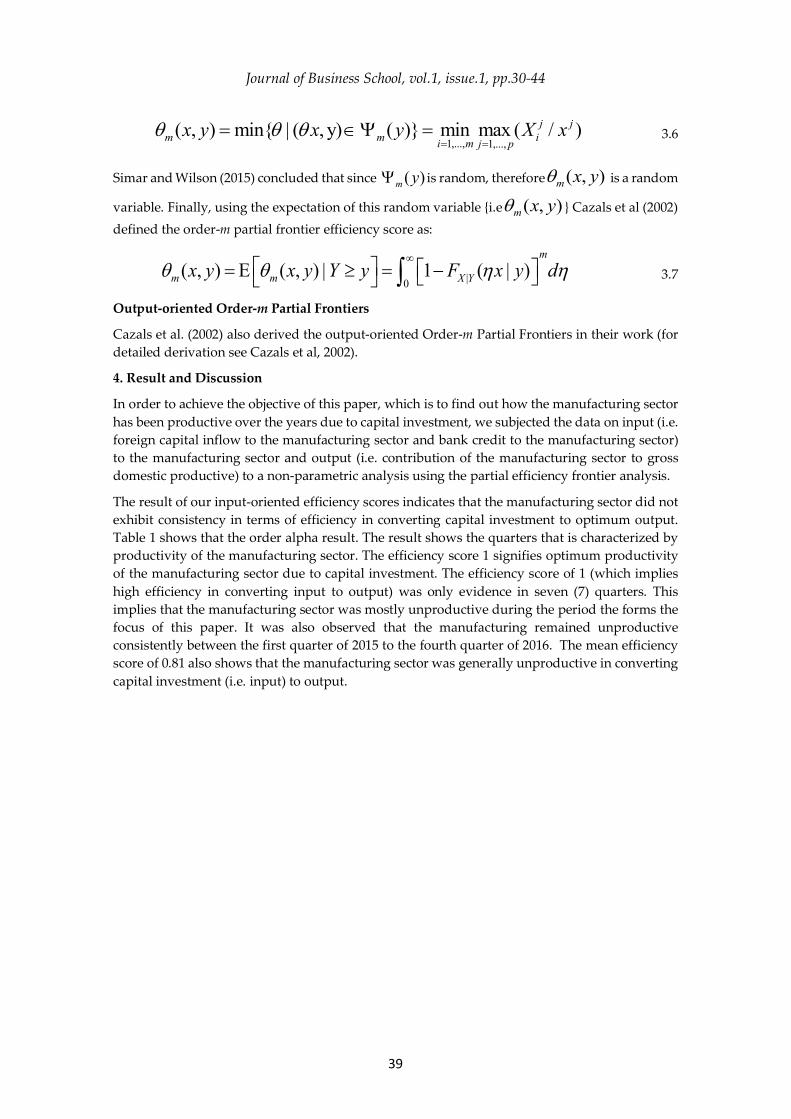
Journal of Business School, vol.1, issue.1, pp.30-‐‑44
39
3.6
Simar and Wilson (2015) concluded that since is random, therefore is a random
variable. Finally, using the expectation of this random variable {i.e } Cazals et al (2002) defined the order-‐‑m partial frontier efficiency score as:
3.7
Output-‐‑oriented Order-‐‑m Partial Frontiers
Cazals et al. (2002) also derived the output-‐‑oriented Order-‐‑m Partial Frontiers in their work (for detailed derivation see Cazals et al, 2002).
4. Result and Discussion
In order to achieve the objective of this paper, which is to find out how the manufacturing sector has been productive over the years due to capital investment, we subjected the data on input (i.e. foreign capital inflow to the manufacturing sector and bank credit to the manufacturing sector) to the manufacturing sector and output (i.e. contribution of the manufacturing sector to gross domestic productive) to a non-‐‑parametric analysis using the partial efficiency frontier analysis.
The result of our input-‐‑oriented efficiency scores indicates that the manufacturing sector did not exhibit consistency in terms of efficiency in converting capital investment to optimum output. Table 1 shows that the order alpha result. The result shows the quarters that is characterized by productivity of the manufacturing sector. The efficiency score 1 signifies optimum productivity of the manufacturing sector due to capital investment. The efficiency score of 1 (which implies high efficiency in converting input to output) was only evidence in seven (7) quarters. This implies that the manufacturing sector was mostly unproductive during the period the forms the focus of this paper. It was also observed that the manufacturing remained unproductive consistently between the first quarter of 2015 to the fourth quarter of 2016. The mean efficiency score of 0.81 also shows that the manufacturing sector was generally unproductive in converting capital investment (i.e. input) to output.
1,..., 1,...,( , ) min{ | ( , y) ( )} min max ( / )j j
m m ii m j px y x y X xq q q
= == ÎY =
( )m yY ( , )m x yq
( , )m x yq
|0( , ) ( , ) | 1 ( | )
m
m m X Yx y x y Y y F x y dq q h h¥
é ù é ù= E ³ = -ë ûë û ò

Journal of Business School, vol.1, issue.1, pp.30-‐‑44
40
Table 1: Order-‐‑alpha Efficiency Result
Note: z-Statistic is abs(Eff.Score - 1)/Std.Err. manoutp_2016q4 .5824295 .0760088 5.493711 23 manoutp 20 manoutp_2016q3 .5934322 .0774447 5.24978 22 manoutp 20 manoutp_2016q2 .6307097 .1045205 3.533185 19 manoutp 20 manoutp_2016q1 .6294503 .0985412 3.760353 20 manoutp 20manoutp_2015q4 .5802345 .0954004 4.400039 24 manoutp 20 manoutp_2015q3 .6467378 .1344657 2.627156 17 manoutp 20manoutp_2015q2 .6094939 .0799175 4.886364 21 manoutp 20 manoutp_2015q1 .6323313 .1036134 3.548466 18 manoutp 20manoutp_2014q4 1 . . 1 manoutp_20manoutp_2014q3 1 .0669563 0 1 manoutp_20manoutp_2014q2 .7118624 .1101408 2.616085 16 manoutp 20 manoutp_2014q1 .763342 .0895384 2.643089 15 manoutp 20manoutp_2013q4 .7713886 .0679196 3.365912 14 manoutp 20 manoutp_2013q3 .8298589 .068407 2.487187 13 manoutp 20 manoutp2013q2 .8406559 .144013 1.106457 11 manoutp 20 manoutp2013q1 1 .1148833 0 1 manoutp201 manoutp2012q4 1 .2133041 0 1 manoutp201 manoutp2012q3 .8308868 .0992702 1.703564 12 manoutp 20 manoutp2012q2 .9990407 .1871565 .0051255 8 manoutp 20 manoutp2012q1 .8779337 .0842247 1.449293 10 manoutp 20 manoutp 2011q4 .9157271 .1854385 .454452 9 manoutp 20 manoutp 2011q3 1 .2457606 0 1 manoutp 20 manoutp 2011q2 1 .2584307 0 1 manoutp 20 manoutp 2011q1 1 .1799798 0 1 manoutp 20 (sector_year) Eff. Score Std. Err. z Stat. Eff. Rank Ref. DMUdmu
Share of efficient dmus = .2917 Median efficiency = .8304 Mean efficiency = .8102 Number of outputs = 1Number of inputs = 2Number of dmus = 24
FDH input-oriented efficiency scores estimated (no variable saved)
. orderalpha sector_year , inp( i_foreigncap i_bankcap ) out( o_manoutp ) reps(200) tab(full) nog

Journal of Business School, vol.1, issue.1, pp.30-‐‑44
41
Table 2: Order-‐‑m Efficiency Result
Table 2 above shows that the order-‐‑m result. The result shows the ranking of quarters that is according to efficiency in productivity of the manufacturing sector. The efficiency rank of 1 (which implies high efficiency in converting input to output) was evident in the first quarter of the year 2011. This implies that the manufacturing sector was most productive during the first quarter of the year 2011. Moreover, the result also shows that the manufacturing sector was very productive between the first and third quarters of the year 2011. It was also observed that the manufacturing sector had its worst ranking during the fourth quarter of 2016. The table as shows that the lowest ranks for the manufacturing sector were evident between the first quarter of 2015 to the fourth quarter of 2016.
.
Note: no bootstrapping; no standard errors computed manoutp_2016q4 .6139045 . . 23 manoutp 20 manoutp_2016q3 .6237598 . . 22 manoutp 20 manoutp_2016q2 .6542923 . . 18 manoutp 20 manoutp_2016q1 .6558717 . . 17 manoutp 20manoutp_2015q4 .5965047 . . 24 manoutp 20 manoutp_2015q3 .6506183 . . 19 manoutp 20manoutp_2015q2 .6438831 . . 20 manoutp 20 manoutp_2015q1 .6393206 . . 21 manoutp 20manoutp_2014q4 1 . . 6 manoutp_20manoutp_2014q3 1 . . 6 manoutp_20manoutp_2014q2 .7350816 . . 16 manoutp 20 manoutp_2014q1 .7933708 . . 15 manoutp 20manoutp_2013q4 .8255089 . . 14 manoutp 20 manoutp_2013q3 .8786153 . . 11 manoutp 20 manoutp2013q2 .8691237 . . 12 manoutp 20 manoutp2013q1 1.000045 . . 5 manoutp201 manoutp2012q4 1.000828 . . 4 manoutp201 manoutp2012q3 .8680405 . . 13 manoutp 20 manoutp2012q2 .9990667 . . 8 manoutp 20 manoutp2012q1 .9196644 . . 10 manoutp 20 manoutp 2011q4 .9283818 . . 9 manoutp 20 manoutp 2011q3 1.001159 . . 3 manoutp 20 manoutp 2011q2 1.02059 . . 2 manoutp 20 manoutp 2011q1 1.022021 . . 1 manoutp 20 (sector_year) Eff. Score Std. Err. z Stat. Eff. Rank Pseudo Refdmu
Share of super-efficient dmus = .2083 Share of efficient dmus = .0833 Median efficiency = .8686 Mean efficiency = .8308 Number of outputs = 1Number of inputs = 2Number of dmus = 24
Order-m(16) input-oriented efficiency scores estimated (variable _om_input_16)
. orderm sector_year , inp( i_foreigncap i_bankcap ) out(o_manoutp) m(16) d(1000) tab(full)

Journal of Business School, vol.1, issue.1, pp.30-‐‑44
42
Conclusion and Recommendations
The literature reviewed so far has shown that productivity of a firm or group of firms making up a specific sector is defined by the ability to efficiently convert capital investment to optimum output. Hence the need to investigate the productivity of the manufacturing sector using the input-‐‑output analysis. From the findings, this study concludes that the manufacturing sector in Nigeria has been unproductive generally when it comes to converting capital investment into optimum output. It is worthy of mention that the sector, at the earliest period covered by the study, performed well but started declining as time passes by. The implication is that the sector has not been unproductive from inception. Rather, this situation may have become evidence due to neglect of the sector by the government. It may also have been due to decay in infrastructural facilities needed to boost the productivity of the sector. This paper therefore recommends appropriate policy capable of providing the manufacturing sector with the enabling environment to thrive better and performance at optimum.
References
Adekoya, A. (1987). The Role of Government in Promoting Increased Productivity on Nigerian Farms. Proceeding of the First National Conference on Productivity, National Productivity Centre, 1991, Page 56.
Akinlo, E. A. (1996). Improving the Performance of the Nigerian Manufacturing Sub-‐‑Sector after Adjustment. The Nigerian Journal of Economic and Social Studies, Page 9.
Aristovnik, A. (2012). Relative Efficiency of Secondary Education: A Comparative Analysis of Slovena and Croatia. Paper presented at the Management, Knowledge and Learning International Conference. Available Online: http://issbs.si/press. Accessed on the 3rd of June 2015.
Baldwin, C. Y., & Clark, K. B. (1992). Capabilities and capital investment: new perspectives on capital budgeting. Journal of Applied Corporate Finance, 5(2), 67-‐‑82.
Barney, J. (1986). Strategic factor markets: expectations, luck and business strategy. Management Science, 32(10), 1231-‐‑1241.
Castejón, C.F. and J., Wörz. (2005). Good or Bad? The Influence of FDI on Output Growth: An industry-‐‑level analysis. WIIW Working Papers No.38.
Cazals, C., Florens,J. P.and Simar,L.(2002). Nonparametric frontier estimation: A robust approach. Journal of Econometrics, 106, pp.1-‐‑25.
Grant, R. M. (1991). The resource-‐‑based theory of competitive advantage: implications for strategy formulation. California Management Review, Spring 1991, 114-‐‑135.
Karl, H. (1988). Financial and Economic Analysis of Enterprises. International Labour Office, Geneva.
Li, X. and Liu, X. (2005). Foreign Direct Investment and Economic Growth: An Increasingly Endogenous Relationship. World Development Report,33(3), pp.393-‐‑407.
Marwah, K. and Tavakoli, A. (2004). The Effect of Foreign Capital and Imports on Economic Growth. Journal of Asian Economics, Vol. 15 pp 399-‐‑413.
Oloko, O. (1983). Factors in Labour Productivity. Proceeding of a National Conference on Productivity, Edited by Osoba, A.M. Page 7.
Osoba, A. M. (Ed.), Productivity in Nigeria. Proceedings of a National Conference organized by PPIPB and NISER, 1983.
Journal of Business School, vol.1, issue.1, pp.30-‐‑44
43
Schroeder, R. G., Bates, K. A., & Junttila, M. A. (2002). A resource-‐‑ based view of manufacturing strategy and the relationship to manufacturing performance. Strategic Management Journal, 23 (2), 105-‐‑117.
Simar, L.and Wilson, P. (2015). Statistical Approaches for Nonparametric Frontier Models: A Guided Tour. In: International Statistical Review, 83(1), p. 77-‐‑110. Available Online: http://hdl.handle.net/2078.1/144745. Access on the 7th of September 2015.
Tang, C.F., W.T. Tan, and I. Ozturk (2016). Energy Consumption and Economic Growth in Vietnam. Renewable and Sustainable Energy Reviews, 54, 1506-‐‑1514.
Udo-‐‑Aka, U. (1983), Measuring productivity: Issues and Problems in Productivity in Nigeria. Proceedings of a National Conference, Edited by Osoba, A.M., Page 75.
USA Business Week (1975). Special Report on Major Business Problems. Page 4.
Vu, T. and Noy, I. (2006). Is Foreign Direct Investment Good for Growth? Answers Using Sectoral Data from China and Vietnam. Unpublished.
Wheelock.,D.C. and Wilson,P.W.(2003). Robust Nonparametric Estimation of Efficiency and Technical Change in U.S. Commercial Banking. Working Paper of Federal Reserve Bank of St. Louis, 037A. http://research.stlouisfed.org/wp/2003/2003-‐‑037.pdf

Journal of Business School, vol.1, issue.1, pp.30-‐‑44
44
Appendix
Period
Capital Importation to the Production/Manufacturing
Sector ($ Million)
Bank Credit to the Manufacturing Sector
(N Million)
Manufacturing Output (N Billion)
2011q1 108.30 1,007,399.05 958,330.55 2011q2 126.12 910,000.42 1,035,168.80 2011q3 201.25 1,087,403.34 1,092,258.19 2011q4 125.72 1,053,213.33 1,130,433.75 2012q1 41.01 1,082,856.40 1,179,096.80 2012q2 198.82 1,088,447.45 1,169,052.70 2012q3 77.61 1,109,775.10 1,245,860.23 2012q4 231.67 1,068,341.70 1,189,649.69 2013q1 169.44 1,067,487.75 1,428,427.98 2013q2 116.33 1,082,488.64 1,433,788.65 2013q3 72.59 1,096,572.48 1,481,916.75 2013q4 32.98 1,179,691.40 1,482,225.07 2014q1 104.07 1,192,126.85 1,648,574.80 2014q2 107.88 1,278,337.60 1,634,725.59 2014q3 365.10 1,323,025.02 1,718,985.30 2014q4 366.92 1,500,625.10 1,681,932.05 2015q1 118.36 1,878,091.98 1,637,067.07 2015q2 51.20 1,909,491.64 1,572,338.22 2015q3 162.42 1,958,451.18 1,688,873.56 2015q4 91.72 1,736,192.99 1,688,339.78 2016q1 77.77 1,862,589.07 1,522,488.04 2016q2 89.42 2,058,036.94 1,519,448.03 2016q3 68.25 2,130,441.30 1,614,894.65 2016q4 67.21 2,215,741.07 1,645,401.73
Source: Central Bank of Nigeria Statistical Bulletin (2016) and National Bureau of Statistics
Annual Abstract of Statistics (2016)

Journal of Business School 2018, 1(1):45-‐‑66
DOI: 10.29226/TR1001.2018.65 Journal Homepage: https://www.journalbusiness.org
An Analysis of Stock Market Anomalies: Evidence from the Nigerian Stock Exchange
Esther Ikavbo EVBAYIRO-‐‑OSAGIE (Ph.D) Department of Banking and Finance, Faculty of Management Sciences, University of Benin, Benin City, [email protected], esther.evbayiro-‐‑[email protected]
Peter O. ERIKI (Ph.D) Department of Banking and Finance, Faculty of Management Sciences, University of Benin, Benin City, [email protected], [email protected]
Abstract
The study examines stock market anomalies in the Nigerian Stock Market (NSE) by investigating month-‐‑of-‐‑the-‐‑year calendar anomalies, size and value fundamental anomalies and momentum effect within asset pricing models. The study also tests for the statistical significance of profit opportunities in anomalies. The sample size is 139 stocks listed on the NSE for the period 2008 to 2015. The time series pooled multiple regression analysis was employed in the study using calendar dummy, the three-‐‑factor model and the four-‐‑factor model. In addition, ten portfolios based on market capitalization, price-‐‑to-‐‑book and price gainers-‐‑to-‐‑losers’ criteria were constructed. The study found that there was no January effect but there was strong evidence of July and August effect on most portfolios formed. The July and August monthly calendar anomalies did not exert a significant influence on all portfolios’ excess returns after controlling for size, value and momentum factors. The findings also revealed that momentum effect was statistically significant in influencing the portfolio excess returns of big and small price winners’ and losers’ portfolios. In the NSE most portfolios constructed had no profit opportunities that are of statistical significance for the period under study. It was recommended that investors and equity portfolio managers should consider buying for their portfolio construction around July and August due to the existence of statistically significant negative returns around those periods. Also, investment fund managers should consider size and value factor as well as momentum factor in the pricing of asset to minimize loss and maximize return.
Keywords: Calendar anomalies, Size and Value effect, Momentum effect, fundamental anomalies, Stock market anomalies

Journal of Business School, vol.1, issue.1, pp.45-‐‑66
46
Introduction
Stock markets and analysis of stock markets have become key issues in most economies of the world because stock market is one of the most sensitive segments of any economy. It is through this segment that the country’s long-‐‑term economic growth and developmental goals are achieved and its exposure to the global economy is most readily felt. The Nigerian Stock Exchange (NSE) was established in 1960 for this purpose and has experienced phenomenal growth and development. The developmental efforts and increased trading activities of the stock exchange are directed towards achieving market efficiency. Market efficiency implies the situation where financial asset’s prices incorporate all available information. It defines the relationship between information and asset prices in the market. Essentially, “the phrase ‘prices fully reflect all available information’ is a statement about two separate aspects of prices, namely: the information content and the price formation mechanism”. It therefore means that any test of this hypothesis “must concern the kind of information reflected in prices, and how this information comes to be reflected in prices” (Lo, 2007:10). However, with frequent and constant releases and dissemination of information in the environment and within firms, efficient markets now seem hard to achieve and even more difficult to maintain. Fama (1991) study reveals various problems with market efficiency such as “deciding what are reasonable information, trading costs and the joint-‐‑hypothesis problem” (p.1575). To Mackey (1841), there is a feeling of something shockingly wrong with the concept of market efficiency. This led to the concept of ‘anomalies’ in stock market and hence ‘anomalies of efficient market hypothesis’. The term ‘anomaly’ can be traced to Field (1934), where stock market seasonality in the form of weekend or holiday effect was first documented.
Stock market anomalies refer to a situation when a security or market performs contrary to the notion of EMH. It can be described as a situation where “market returns are not consistent with the traditional asset pricing behaviour” (Bundoo, 2011:5) and where, as put further by Shiller (2001), the principle of rational behaviour by investors is not entirely correct. There are many stock market anomalies, some occur once or twice and disappear, while others are continuous (Archana, Safeer & Kevin, 2014). Stock market anomalies could be related to calendar anomalies Field (1934), size effect and value effect (Keim, 1983) which are called fundamental anomalies; announcement anomalies and technical trading rules anomalies in form of momentum effect. Anomalies can affect the market as well as influence investors’ decisions and behaviour in the market. Investors are always conscious of their returns and will usually want to predict returns in the market as a reward for their investment. If stock markets are efficient, investors in stock cannot expect to realize superior profits from market anomalies.
Numerous studies on stock market anomalies have been conducted and reported for developed and some emerging stock markets. For developed markets in US, Canada, UK, Japan, Australia and Hong Kong; anomalies such as calendar anomalies (in form of turn-‐‑of-‐‑the-‐‑year effect, month-‐‑of-‐‑the-‐‑year effect, day-‐‑of-‐‑the-‐‑week effect); size and value fundamental anomalies have been continuously observed (Banz, 1981; Keim, 1983; Jaffe & Westerfield, 1985). This is also the case for some emerging markets such as Indian Stock Exchange (Dash, Dutta & Sabaharwal, 2011); the Stock Exchange of Mauritius (Bundoo, 2011); Ghana Stock Exchange (Alagidede & Panagiotidis, 2012). Despite the numerous research works on stock market anomalies globally, the analysis of stock market anomalies in the Nigerian Stock Exchange is limited and yet to be established. These few studies (Chukwuogor-‐‑Ndu, 2007; Idolor, Ogieva & Osamwonyi, 2014) have examined either a single or a few market anomalies in the Nigerian Stock Exchange. As a result, this study fills the gap in empirical literature by examining three stock market anomalies using common stocks listed in the NSE as it is one of the fastest growing emerging markets in Africa. Significantly, the present study examines stock market anomalies within an asset pricing
Journal of Business School, vol.1, issue.1, pp.45-‐‑66
47
model framework by employing Fama and French (1993) three-‐‑factor model and the four-‐‑factor model by Carhart (1997) in an emerging market context, why previous studies have either used the market model, GARCH or ARCH approach or the traditional asset pricing model (like CAPM) in analysing market anomalies. The study is therefore timely given the scarcity of research with these models in the Nigerian Stock Market.
Therefore, the objectives of this study are to 1. examine whether month-‐‑of-‐‑the-‐‑year calendar anomalies are present in the Nigerian Stock Market, particularly when controlling for systematic risk; 2. examine whether size effect and value effect fundamental anomalies are present in the Nigerian Stock Market; 3. investigate if momentum effect are present in the Nigerian Stock Market after controlling for size and value; and 4. investigate if month-‐‑of-‐‑the-‐‑year calendar anomalies persist when the size, value and momentum factors are controlled for.
Review of Related Literature
Returns represent the reward or income or capital gain derived for undertaking investment. It is the primary motivating factor that drives investment in the capital market. For returns, investors need to almost invariably bear some risk. Importantly, the differences in the distribution of returns for each stock with respect to month-‐‑of-‐‑the-‐‑year, firm’s size and value will enable investors to invest in stocks and adjust their portfolios when necessary. When investors notice a pattern in the distribution of returns, they see an opportunity to earn profit by trading on the information. This leads to abnormal return. Abnormal return is the anomalous or irregular profit earned by trading on information in the market. Abnormal equity returns are associated with stock market anomalies. According to Jacobs & Levy (1988) these returns are not unique to one historical period, nor can they be explained by consideration of risk or value.
From financial literature, there are significant deviations from efficient market hypothesis otherwise known as anomalies (Fama, 1991). Lo (2007) refers to anomalies as perhaps the most common challenge to Efficient market hypotheses (EMH). Stock market anomalies have been one of the interesting areas of financial market research in the last four decades as the presence of these phenomena has been evident in developed capital markets. Keim (2007) explains it as a “regular pattern in an asset’s returns” which is regular, reliable and widely known. Also, he explains that “the fact that the pattern is regular and reliable implies a degree of predictability, and the fact that the regularity is widely known implies that many investors can take advantage of it” (Keim, 2007: 7-‐‑8). It can also be described “as empirical results or market returns that are not consistent with the traditional or maintained theories of asset pricing behaviour” (Bundoo, 2011:5). It therefore means that stock market anomalies will show either stock market inefficiency (that is, profit opportunities) or “inadequacies in the underlying asset-‐‑pricing model” (Schwert, 2003:947). To this end, there are two aspects of stock market anomalies: The first aspect says that stock market anomalies can be as a result of opportunities to earn abnormal profits from the trading activities of an investor. And the second aspect says that stock market anomalies can arise because the underlying asset-‐‑pricing model is faulty. Stock market anomalies could be in the form of calendar effects, fundamental effect, and technical trading rules. To Keim (2007), they could be cross-‐‑sectional with cross-‐‑sectional return pattern or time series with time-‐‑series return pattern in nature.
Calendar Anomalies Calendar anomalies are anomalies or market inefficiencies that are linked to a particular time. It can also be described as stock prices anomalies or stock return changes that are attributable to calendar. The existence of this anomaly is a denial of the weak-‐‑form of EMH which states that stock prices reflect all past information. It also depicts that returns are invariant, meaning that there exist short term seasonal pattern in stock returns (Mishra, 2012). This implies seasonality in stock market. Nonetheless, evidence overtime suggests that stock

Journal of Business School, vol.1, issue.1, pp.45-‐‑66
48
returns do not remain constant and that the market can be outperformed by means of calendar or seasonal dummies. The months-‐‑of-‐‑the-‐‑year effect or January calendar effect according to Fama (1991:1586-‐‑1587) is “the most mystifying seasonal”. Stock returns, especially returns on small stocks, are on average higher in January than in other months”. January returns are usually positive and significantly higher than other months of the year. A look at several studies in seasonality of return show that the end of the year’s effect most commonly referred to as January effect is the most prominent of all monthly calendar anomalies (Mills & Counts, 1995; Ali & Akbar, 2008). It describes the propensity for stock prices to rise during the trading period beginning with the last trading day in December and ending on the last trading day in January. The work of Wachtel (1942) is the first study to discover January effect on stock markets. The January effect seems robust to sampled period, and it is difficult to reconcile with the EMH because of its persistence, regularity and publicity (Lo, 2007). Li (2013) reports five common explanations for the January effect to be: (1) the tax loss hypothesis (tax-‐‑loss selling at year end); (2) the inter-‐‑generational transfer hypothesis (Gamble, 1993); (3) information release during this period; (4)the Capital Asset Pricing Model (CAPM) mis-‐‑specification; and (5) institutional investors’ behaviour. Other possible reasons are trade and settlement date delay; shift in the information processing hypothesis (Miller, 1988); as well as risk-‐‑based theory.
Many research studies have been carried out to explore and empirically test the presence of calendar anomalies in the developed markets and some emerging markets but very few exist on the Nigerian Stock Exchange. Although these studies reported mix results but most works support the fact that January returns tend to be higher than other months returns. Evidence generated from studies of Jaffe and Westerfield (1985), Anderson, Gerlach and Di Traglia (2003) and Schwert (2003) on the US markets show the presence of January effect -‐‑ that on the average, stock returns in January are usually higher than other months of the year. An elaborate study by Hansen and Lunde (2003) on 10 countries stock markets (including US) shows that month-‐‑of-‐‑the-‐‑year effects were significantly present in almost all the markets. However, the work of Li (2013) on Canada finance industry found a weak January effect and thus concluded that there are no abnormal returns to take advantage of the January anomaly. Considering studies on emerging markets, Bundoo (2011) studied the Stock Exchange of Mauritius and reports a very minimal January effect both at the market and company level. Further investigation reveals that the market has a strong September effect. Similarly, Alagidede and Panagiotidis (2012) on the Ghanaian capital market discover April effect contrary to the January effect pattern in most markets. Likewise, Stoica and Diaconasu (2012) work on emerging Central and Eastern European stock markets for the period 2000 to 2010, report the existence of January effect in Czech Republic, Croatoa, Macedonia, Romania, Slovenia and Hungary. Kuria and Riro (2013) studied the Nairobi Securities Exchange and found the presence of seasonal effects in the market. On the other hand, studies by Maghayereh (2003) on the Amman Stock Exchange in Jordan and Silva (2010) on the Portuguese Stock Exchange document no evidence of month-‐‑of-‐‑the-‐‑year or January effect in these emerging markets. Also, Singh (2014) did an elaborate study on emerging BRIC markets (Brazil, Russia, India and China market) and the results obtained demonstrate a non significant month-‐‑of-‐‑the-‐‑year calendar effect in the Brazil, Russia and India markets. For African and Nigerian markets, the work of Ayadi (1998) on low-‐‑income African emerging markets reported the presence of seasonality (January effect) in stock returns on the Nigerian, Ghanaian and Zimbabwean stock markets. Correspondingly Idolor et al (2014), in their study on the Nigerian Stock Market using monthly market index from 2005 to 2010 show that the months of February, March, April, May and December were consistently associated with negative market returns. While the months of January, August, September, October and November were associated with positive returns.

Journal of Business School, vol.1, issue.1, pp.45-‐‑66
49
Fundamental (Value and Size) Effect: Under the fundamental anomalies, this study pays attention to the size and value effect. Size effect is one of the most enduring anomaly in the market – “it is the apparent excess expected returns that accrue to stocks of small-‐‑capitalization companies in excess of their risks” (Lo.2007:8). Size effect can be described as the anomaly where small firms (those with small market capitalizations) outperform large firms (those with large market capitalizations) (Hodnett & Hsieh, 2012). In order words, the size effect is the empirical regularity that firms with small market capitalization exhibit returns that on the average significantly exceed those of large firms.
The value effect can be described as the positive relation between security returns of value securities to the market price of securities (Keim, 2007). It also means that positive abnormal risk-‐‑adjusted returns accrue to value stocks, which are stocks possessing high ratios of fundamental values relative to their share prices. Many research studies reveal that positive abnormal returns seem to accrue to portfolio of stocks with low price-‐‑to-‐‑book value, high book-‐‑to-‐‑market value (B/M), high earnings-‐‑to-‐‑price (E/P) ratios or high dividend yields (Basu, 1983; Schwert, 2003). The low price-‐‑to-‐‑book (otherwise high book-‐‑to-‐‑market) value firms are underpriced by the market and have high book value. They are then a good buy and hold targets as their prices will possibly rise with time. These fundamental anomalies undermine the semi-‐‑strong form of market efficiency. Possible explanations have been suggested for the size and value effect. According to Ball (1978), these explanations are likely to indicate inadequacy in the underlying asset pricing model rather than market inefficiency. They are (1) Small firm’s stocks are more illiquid with higher transaction costs; (2) there are some unique risks associated with small size firms [e.g lower operating efficiency, higher leverage]; (3) there are limited information available about small firms; (4) small firm’s stocks trade less regularly than large firm’s stocks, hence their beta estimates might be less dependable; (5) the value premium (BE/ME) anomaly is not an anomaly parse but a premium or compensation for risk; (6) the value premium is also due to investors’ overreaction to firm performance; and (7) the value premium is due to the value characteristic and not risk.
The size and value effects have been investigated and reproduced by numerous researchers for different sampled periods for most developed and few developing securities markets around the world. Some studies on the US stock market have reported the side and value effect. Rozeff and Kinney (1976) and Banz (1981) in their respective studies, document that small capitalization stocks tend to outperform large capitalization stocks by a wide margin. Keim (1983) work reports that the relation between daily abnormal returns and size is negative and more in January than other months of the year. Similarly, in the work of Fama and French (1995) specifically discovered a negative relation between cross section of average returns and firm size, and a positive relation between cross section of average returns and firm’s book-‐‑to-‐‑value equity ratios. Equally, empirical works in emerging markets have documented the size and value effect. Drew and Veeraraghavan (2002) document evidence of the size and value effect for the Kuala Lumpur Stock Exchange. Bundoo (2011), studied the Stock Exchange of Mauritius and the findings indicate that the size and value premium subsumed most of the day-‐‑of-‐‑the-‐‑week effects. Li (2013) study on Canada finance industry found a weak January effect in small-‐‑cap firms.
Technical Trading Rules (Momentum Effect): It has been observed that security with “prices on an upward or downward trajectory over a period of 3 to 12 months have a higher than expected probability of continuing on that upward or downward trajectory over the subsequent 3 to 12 months”. The display of this temporal pattern in prices of securities is known as momentum (Keim, 2007:5). Momentum effect is the “effect that over intermediate horizons, winners stocks continue to perform well and losers stocks continue to perform poorly” (Glaser
Journal of Business School, vol.1, issue.1, pp.45-‐‑66
50
& Weber, 2003:108). It occurs when past equity returns are used as explanatory variables in the cross-‐‑section of stock returns. Likely acceptable explanations provided for momentum effects are: (1) data Snooping Bias; (2) reward for risk; (3) Trading behaviour of investors; and (4) Cross-‐‑sectional difference in expected returns.
There have been persistent momentum effects (profits) as verified from developed capital markets. Hong, Lim and Stein (2000), Jegadeesh (1990), Jegadeesh and Titman (1993, 2001) studied the US markets and Nijman, Swinkels and Verbeek (2004) studied the European stock market. In their individual research work, they examined momentum returns to firm size and value and found that momentum effect is more in small cap stocks in the respective markets studied. Jegadeesh (1990) reports that stocks that have performed well over the past few months tend to make high returns over the next months. In a follow-‐‑up study, Jegadeesh and Titman (1993) show that a strategy that simultaneously buys past winners and sells past losers produces significant abnormal returns over holdings periods of 3 to 12 months that is independent of market, size or value factors. In another study by Jegadeesh and Titman (2001), the findings show that momentum effect is more pronounce for small cap stocks. This again confirms the results of their earlier study. Carhart (1997) investigated momentum for a sample of mutual funds companies. The results indicate that the momentum factor was statistically significant along with the size and value factors. Chan, Hameed and Tong (2000) in their study on international equity market, found the momentum effect to be significant with a t value of 2.35. Subsequently, Hong et al (2000), investigated return momentum effect on the basis of size and found that portfolio of stocks with the highest market value has non-‐‑existent of momentum effect. Nijman et al (2004) in their study of the European stock market, investigated momentum effect on the basis of size and value and the results indicate that momentum effect is more for small growth stocks. Furthermore, They reported momentum profits for China market only. Israel and Moskowitz (2013) examined the last century in US stock markets and the last four decades in the international stock markets. They documented that momentum profits are present in every size group across the markets studied.
Theoretical Framework: In general, the modern capital market theories that provide explanations to stock market anomalies can be classified into two: risk-‐‑based or rational theories and the non-‐‑risk-‐‑based or behaviour theories. Drawing from the rational theories, the study adopts the three-‐‑factor model and the four-‐‑factor model. The three-‐‑factor model is a multifactor model developed by Fama and French in 1992, which is a microeconomic based risk factor. The model helps to overcome the inability of the CAPM in explaining size effect, value effect and other obvious anomalies. Before the Fama and French three-‐‑factor model, several research studies [such as Keim (1983, Cook and Rozeff (1984)] have documented evidence of firm characteristics (firm size, earnings-‐‑to-‐‑price ratio, book-‐‑to-‐‑equity ratio (BE/ME), price-‐‑to-‐‑book value (P/B) and past sales growth) explaining on the average stock returns that cannot be explained by the CAPM. Similarly, Carhart (1997) developed the four-‐‑factor model, which included an additional factor called the momentum factor to the Fama and French three-‐‑factor model. The four-‐‑factor model is consistent with a model of market equilibrium with four risk factors. This additional momentum factor was motivated by the inability of the three-‐‑factor model to explain cross-‐‑sectional variables in returns in portfolio sorted by momentum.
From the literature review especially empirical literature, it is obvious that most of the studies on stock market anomalies have been predominantly carried out in developed markets (US, Australian) and some emerging markets (Asian, Kenya, South Africa). However, investigating stock market anomalies with the application of Fama and French three factor model and Carhart’s four-‐‑factor model have not be fully and predominantly done in the Nigerian market. Hence, the need to study month-‐‑of-‐‑the-‐‑year anomalies on portfolio’s bases, size and value effect
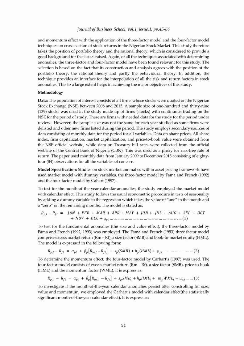
Journal of Business School, vol.1, issue.1, pp.45-‐‑66
51
and momentum effect with the application of the three-‐‑factor model and the four-‐‑factor model techniques on cross-‐‑section of stock returns in the Nigerian Stock Market. This study therefore takes the position of portfolio theory and the rational theory, which is considered to provide a good background for the issues raised. Again, of all the techniques associated with determining anomalies, the three-‐‑factor and four-‐‑factor model have been found relevant for this study. The selection is based on the fact that its construction and analysis agrees with the position of the portfolio theory, the rational theory and partly the behavioural theory. In addition, the technique provides an interface for the interpolation of all the risk and return factors in stock anomalies. This to a large extent helps in achieving the major objectives of this study.
Methodology
Data: The population of interest consists of all firms whose stocks were quoted on the Nigerian Stock Exchange (NSE) between 2008 and 2015. A sample size of one-‐‑hundred and thirty-‐‑nine (139) stocks was used in the study made up of firms (stocks) with continuous trading on the NSE for the period of study. These are firms with needed data for the study for the period under review. However, the sample size was not the same for each year studied as some firms were delisted and other new firms listed during the period. The study employs secondary sources of data consisting of monthly data for the period for all variables. Data on share prices, All share index, firm capitalization, market capitalization, and price-‐‑to-‐‑book value were obtained from the NSE official website, while data on Treasury bill rates were collected from the official website of the Central Bank of Nigeria (CBN). This was used as a proxy for risk-‐‑free rate of return. The paper used monthly data from January 2009 to December 2015 consisting of eighty-‐‑four (84) observations for all the variables of concern.
Model Specification: Studies on stock market anomalies within asset pricing framework have used market model with dummy variables, the three-‐‑factor model by Fama and French (1992) and the four-‐‑factor model by Cahart (1997).
To test for the month-‐‑of-‐‑the-‐‑year calendar anomalies, the study employed the market model with calendar effect. This study follows the usual econometric procedure in tests of seasonality by adding a dummy variable to the regression which takes the value of “one” in the month and a “zero” on the remaining months. The model is stated as:
𝑅",$ − 𝑅&$ = 𝐽𝐴𝑁 + 𝐹𝐸𝐵 + 𝑀𝐴𝑅 + 𝐴𝑃𝑅 + 𝑀𝐴𝑌 + 𝐽𝑈𝑁 + 𝐽𝑈𝐿 + 𝐴𝑈𝐺 + 𝑆𝐸𝑃 + 𝑂𝐶𝑇 + 𝑁𝑂𝑉 + 𝐷𝐸𝐶 + µμ"$ …………………………………………… . . .… (1)
To test for the fundamental anomalies (the size and value effect), the three-‐‑factor model by Fama and French (1992, 1993) was employed. The Fama and French (1993) three factor model comprise excess market return (Rm – Rf), a size factor (SMB) and book-‐‑to-‐‑market equity (HML). The model is expressed in the following form:
𝑅",$ – 𝑅&$ = 𝛼"$ + 𝛽"E𝑅F,$ –𝑅&$G + 𝑠"(𝑆𝑀𝐵) + ℎ"(𝐻𝑀𝐿)+ µμ"$ ……………………(2)
To determine the momentum effect, the four-‐‑factor model by Carhart’s (1997) was used. The four-‐‑factor model consists of excess market return (Rm – Rf), a size factor (SMB), price-‐‑to-‐‑book (HML) and the momentum factor (WML). It is express as:
𝑅",$ − 𝑅&$ = 𝛼"$ + 𝛽"E𝑅F,$ − 𝑅&$G + 𝑠"𝑆𝑀𝐵$ + ℎ"𝐻𝑀𝐿$ + 𝑚"𝑊𝑀𝐿$ + µμ",$ ……(3)
To investigate if the month-‐‑of-‐‑the-‐‑year calendar anomalies persist after constrolling for size, value and momentum, we employed the Carhart’s model with calendar effect(the statistically significant month-‐‑of-‐‑the-‐‑year calendar effect). It is express as:
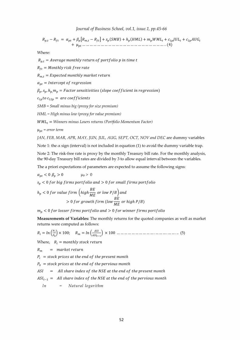
Journal of Business School, vol.1, issue.1, pp.45-‐‑66
52
𝑅",$ − 𝑅&$ = 𝛼"$ + 𝛽"E𝑅F,$ − 𝑅&$G + 𝑠"(𝑆𝑀𝐵) + ℎ"(𝐻𝑀𝐿) +𝑚"𝑊𝑀𝐿$ + 𝑐P"𝐽𝑈𝐿$ + 𝑐Q"𝐴𝑈𝐺$+ µμ"$ ………………………………………………………… . . (4)
Where:
𝑅",$ = 𝐴𝑣𝑒𝑟𝑎𝑔𝑒 𝑚𝑜𝑛𝑡ℎ𝑙𝑦 𝑟𝑒𝑡𝑢𝑟𝑛 𝑜𝑓 𝑝𝑜𝑟𝑡𝑓𝑜𝑙𝑖𝑜 𝑝 𝑖𝑛 𝑡𝑖𝑚𝑒 𝑡
𝑅&$ = 𝑀𝑜𝑛𝑡ℎ𝑙𝑦 𝑟𝑖𝑠𝑘 𝑓𝑟𝑒𝑒 𝑟𝑎𝑡𝑒
𝑅F,$ = 𝐸𝑥𝑝𝑒𝑐𝑡𝑒𝑑 𝑚𝑜𝑛𝑡ℎ𝑙𝑦 𝑚𝑎𝑟𝑘𝑒𝑡 𝑟𝑒𝑡𝑢𝑟𝑛
𝛼"$ = 𝐼𝑛𝑡𝑒𝑟𝑐𝑒𝑝𝑡 𝑜𝑓 𝑟𝑒𝑔𝑟𝑒𝑠𝑠𝑖𝑜𝑛
𝛽", 𝑠", ℎ",𝑚" = 𝐹𝑎𝑐𝑡𝑜𝑟 𝑠𝑒𝑛𝑠𝑖𝑡𝑖𝑣𝑖𝑡𝑖𝑒𝑠 (𝑠𝑙𝑜𝑝𝑒 𝑐𝑜𝑒𝑓𝑓𝑖𝑐𝑖𝑒𝑛𝑡 𝑖𝑛 𝑟𝑒𝑔𝑟𝑒𝑠𝑠𝑖𝑜𝑛)
𝑐P"𝑡𝑜 𝑐PQ" = 𝑎𝑟𝑒 𝑐𝑜𝑒𝑓𝑓𝑖𝑐𝑖𝑒𝑛𝑡𝑠
SMB = Small minus big (proxy for size premium)
HML = High minus low (proxy for value premium)
𝑊𝑀𝐿$ = Winners minus Losers returns (Portfolio Momentum Factor)
µμ"$ = error term
JAN, FEB, MAR, APR, MAY, JUN, JUL, AUG, SEPT, OCT, NOV and DEC are dummy variables
Note 1: the α sign (interval) is not included in equation (1) to avoid the dummy variable trap.
Note 2: The risk-‐‑free rate is proxy by the monthly Treasury bill rate. For the monthly analysis, the 90-‐‑day Treasury bill rates are divided by 3 to allow equal interval between the variables.
The a priori expectations of parameters are expected to assume the following signs:
𝛼"$ < 0 𝛽" > 0 µμp > 0
𝑠" < 0 𝑓𝑜𝑟 𝑏𝑖𝑔 𝑓𝑖𝑟𝑚𝑠 𝑝𝑜𝑟𝑡𝑓𝑜𝑙𝑖𝑜 𝑎𝑛𝑑 > 0 𝑓𝑜𝑟 𝑠𝑚𝑎𝑙𝑙 𝑓𝑖𝑟𝑚𝑠 𝑝𝑜𝑟𝑡𝑓𝑜𝑙𝑖𝑜
ℎ" < 0 𝑓𝑜𝑟 𝑣𝑎𝑙𝑢𝑒 𝑓𝑖𝑟𝑚 iℎ𝑖𝑔ℎ𝐵𝐸𝑀𝐸 𝑜𝑟 𝑙𝑜𝑤 𝑃/𝐵
l𝑎𝑛𝑑
> 0 𝑓𝑜𝑟 𝑔𝑟𝑜𝑤𝑡ℎ 𝑓𝑖𝑟𝑚 (𝑙𝑜𝑤𝐵𝐸𝑀𝐸 𝑜𝑟 ℎ𝑖𝑔ℎ 𝑃/𝐵)
𝑚" < 0 𝑓𝑜𝑟 𝑙𝑜𝑠𝑠𝑒𝑟 𝑓𝑖𝑟𝑚𝑠 𝑝𝑜𝑟𝑡𝑓𝑜𝑙𝑖𝑜 𝑎𝑛𝑑 > 0 𝑓𝑜𝑟 𝑤𝑖𝑛𝑛𝑒𝑟 𝑓𝑖𝑟𝑚𝑠 𝑝𝑜𝑟𝑡𝑓𝑜𝑙𝑖𝑜
Measurements of Variables: The monthly returns for the quoted companies as well as market returns were computed as follows:
𝑅m = 𝑙𝑛 nopoqr × 100; 𝑅F = 𝑙𝑛 n uvw
uvwxyzr × 100 ………………………… .……… .…… . .. (5)
Where, 𝑅m = 𝑚𝑜𝑛𝑡ℎ𝑙𝑦 𝑠𝑡𝑜𝑐𝑘 𝑟𝑒𝑡𝑢𝑟𝑛
𝑅F = 𝑚𝑎𝑟𝑘𝑒𝑡 𝑟𝑒𝑡𝑢𝑟𝑛
𝑃m = 𝑠𝑡𝑜𝑐𝑘 𝑝𝑟𝑖𝑐𝑒𝑠 𝑎𝑡 𝑡ℎ𝑒 𝑒𝑛𝑑 𝑜𝑓 𝑡ℎ𝑒 𝑝𝑟𝑒𝑠𝑒𝑛𝑡 𝑚𝑜𝑛𝑡ℎ
𝑃{ = 𝑠𝑡𝑜𝑐𝑘 𝑝𝑟𝑖𝑐𝑒𝑠 𝑎𝑡 𝑡ℎ𝑒 𝑒𝑛𝑑 𝑜𝑓 𝑡ℎ𝑒 𝑝𝑒𝑟𝑣𝑖𝑜𝑢𝑠 𝑚𝑜𝑛𝑡ℎ
𝐴𝑆𝐼 = 𝐴𝑙𝑙 𝑠ℎ𝑎𝑟𝑒 𝑖𝑛𝑑𝑒𝑥 𝑜𝑓 𝑡ℎ𝑒 𝑁𝑆𝐸 𝑎𝑡 𝑡ℎ𝑒 𝑒𝑛𝑑 𝑜𝑓 𝑡ℎ𝑒 𝑝𝑟𝑒𝑠𝑒𝑛𝑡 𝑚𝑜𝑛𝑡ℎ
𝐴𝑆𝐼$|P = 𝐴𝑙𝑙 𝑠ℎ𝑎𝑟𝑒 𝑖𝑛𝑑𝑒𝑥 𝑜𝑓 𝑡ℎ𝑒 𝑁𝑆𝐸 𝑎𝑡 𝑡ℎ𝑒 𝑒𝑛𝑑 𝑜𝑓 𝑡ℎ𝑒 𝑝𝑒𝑟𝑣𝑖𝑜𝑢𝑠 𝑚𝑜𝑛𝑡ℎ
ln = Natural logarithm

Journal of Business School, vol.1, issue.1, pp.45-‐‑66
53
Portfolios Classification: Size Classification: The stocks used in this study were divided into two classes on the basis of Market capitalization, namely: Small Size Portfolios (stock of small market equity) and Big Size Portfolios (stock of big market equity).
Value (Price-‐‑to-‐‑Book -‐‑ P/B) Classification: Using Fama and French (1993) methodology, the firms was ranked and classified into three groups following the P/B ratio calculated. The price to book value (P/B) rather than boo-‐‑to-‐‑market equity (BE/ME) was used in this study. The use of P/B is based on the popularity and easy of accessing this information by equity investors. The first group created is called High P/B (also called low BE/ME). This consists of all stocks that were above 70 percent of the overall market P/B median. The second group is Medium P/B ratio, and it is made up of stocks that were between 70 percent and 50 percent. The third group is the Low P/B ratio (also called High BE/ME), and it consists of all stocks that were below 50%. Fama and French (1993) posit that the split of stocks into these different categories (two ME groups and three BE/ME groups) was arbitrary. Arguing further, they say that there are no reasons why the test would be sensitive to this choice. Drawing from this argument and on the basis of 2 MC and 3 P/B groups, 6 portfolios where formed: SL, SM, SH, BL, BM and BH.
Where: SL (all stocks in the small market cap group that are also in the low P/B group); SM (all stocks in the small market cap group that are also in the medium P/B group); SH (all stocks in the small market cap group that are also in the high P/B group); BL (all stocks in the large market cap group that are also in the low P/B group); BM (all stocks in the large market cap group that are also in the medium P/B group); and BH (all stocks in the large market cap group that are also in the high P/B group).
Momentum Classification: it was investigated within two separate groups. Firstly, stocks were sorted on the basis of cumulative monthly returns -‐‑ into two groups based on return: the price gainers/winners (also called good performer) (PW) they are stocks with positive annual stock returns and the price losers (poor performer) (PL) they are stocks with negative annual stock returns. Secondly, stocks were arranged on the basis of market cap (size) -‐‑ stocks were classified into two groups: small cap group and big market cap group. Drawing from the argument of Jegadeesh and Titman (1993) and on the basis of two size and two return groups, four portfolios were formed: BPW, BPL, SPW & SPL. Where, BPW (all stocks in the large market cap group and also in the price winners [PW] group); BPL (all stocks in the large market cap group that are also in the PL group); SPW (all stocks in the small market cap group and also in the PW group) and SPL (all stocks in the small market cap group and also in the PL group)
In summary,
§ The portfolio monthly return (Rpt) [the monthly return of each portfolio] is the value-‐‑weighted return of all stock in the portfolio. It is estimated as
𝑅"$ = }𝑊𝑖, 𝑡 ∗ 𝑅𝑖, 𝑡�
$�P
…………………………………………………………… . . … (6)
Where, Rpt = Monthly portfolio p return; Ri,t = stock i return in time t
Wi,t = Weight of stock i in the portfolio (market value of stock i/total market value of portfolio); n = the number of stocks in portfolio p
§ SMB (Small minus Big): SMB for each month represents the difference between each month average returns of small MC group and big MC group. It is expressed as:
SMB = 1/3(SL + SM + SH) – 1/3(BL + BM + BH)……………………. (7)

Journal of Business School, vol.1, issue.1, pp.45-‐‑66
54
§ HML (High minus Low): HML for each month represents the difference between each month’s average returns of high P/B group and low P/B group. It is expressed as:
HML = ½ (BH + SH) – ½ (BL + SL)……………………………….… (8)
§ WML (Winners minus Losers): WML for each month represents the difference between each month average stock returns of price winners group and price losers group.
WML = 1/2(BW + SW) – 1/2(BL + SL)…………………………... (9)
The StataC 13 statistical and econometric software was used as an aid for the analysis. This enables the regression results from the six portfolios to be obtained in one output for each model.
Results and Discussion
Model 1 on the Test for month-‐‑of-‐‑the-‐‑year Calendar anomalies results are reported in table 1 below. The summarized results show that there is no significant January effect for all the portfolios and the January effect factor coefficient is positive for three portfolios. The February effect, April effect, May effect, June effect, September effect and October effect factor coefficients are not significant for all portfolios in the market. The March effect, November effect and December effect factor coefficients are significant in only one portfolio each. March effect has negative factor loading of -‐‑0.04 on SH portfolio. November effect factor loads negatively on SH (-‐‑0.06) portfolio. December effect has positive factor loading of 0.24 on BL portfolio. They all are statistically significant at 5% level. This means that negative returns can be generated from portfolios investment on BH and SH portfolios in the months of March and November respectively. Also positive returns can be generated from trading on BL portfolios in the month of December in Nigerian market. Importantly, the July effect factor coefficients are statistically significant at 5% level for three portfolios, namely SL, SH, and BH portfolios with negative factor loading of -‐‑0.06, -‐‑0.05, and -‐‑0.08 respectively. This means that negative returns can be generated from portfolios investment on small size portfolios (SL, SH) as well as BH in the month of July.

Journal of Business School, vol.1, issue.1, pp.45-‐‑66
55
Table: 1 Test for Monthly Calendar anomalies
JAN FEB MAR APR MAY JUN JUL AUG SEPT OCT NOV DEC
BL-‐‑Rf
SL-‐‑Rf
SH-‐‑Rf
BH-‐‑Rf
BM-‐‑Rf
SM-‐‑Rf
-‐‑0.23 (0.81)
0.01 (0.61)
-‐‑0.00 (0.77)
0.00 (0.92)
0.03 (0.47)
-‐‑0.00 (0.92)
0.36 (0.71)
0.45 (0.20)
0.39 (0.16)
-‐‑0.08 (0.07)
0.06 (0.19)
0.07 (0.06)
-‐‑.098 (0.32)
-‐‑0.52 (0.14)
-‐‑0.04 (0.09)
-‐‑0.08
(0.04)**
-‐‑0.04 (0.40)
-‐‑0.02 (0.46)
-‐‑0.03 (0.76)
-‐‑0.01 (0.65)
-‐‑0.04 (0.09)
-‐‑0.01 (0.72)
0.08 (0.10)
-‐‑0.06 (0.10)
0.07 (0.42)
-‐‑0.01 (0.69)
-‐‑0.02 (0.09)
-‐‑0.02 (0.62)
0.04 (0.39)
0.05 (0.18)
-‐‑0.82 (0.40)
-‐‑0.24 (0.49)
-‐‑0.05 (0.05)
-‐‑0.01 (0.70)
-‐‑0.08 (0.12)
-‐‑0.06 (0.08)
-‐‑0.53 (0.58)
-‐‑0.06
(0.05)**
-‐‑0.05 (0.05)**
-‐‑0.08
(0.05)**
-‐‑0.04 (0.38)
-‐‑0.06 (0.07)
-‐‑0.99 (0.31)
-‐‑0.06 (0.08)
-‐‑0.06
(0.03)**
-‐‑0.13 (0.00)*
-‐‑0.08 (0.08)
-‐‑0.07
(0.05)**
-‐‑0.11 (0.90)
-‐‑0.01 (0.77)
-‐‑0.04 (0.12)
-‐‑0.07 (0.08)
-‐‑0.05 (0.26)
-‐‑0.01 (0.66)
-‐‑0.01 (0.84)
-‐‑0.04 (0.16)
-‐‑0.04 (0.12)
-‐‑0.05 (0.25)
-‐‑0.03 (0.50)
-‐‑0.03 (0.33)
-‐‑0.03 (0.69)
-‐‑0.05 (0.14)
-‐‑0.06
(0.02)**
-‐‑0.03 (0.41)
-‐‑0.07 (0.15)
-‐‑0.05 (0.14)
0.24
(0.01)**
-‐‑0.04 (0.25)
-‐‑0.05 (0.07)
-‐‑0.00 (0.82)
-‐‑0.03 (0.49)
-‐‑0.02 (0.57)
Note: ( ) p-‐‑value, Source: Author’s Computation (2016) with StataC 13; NB: *, ** represent significant at 1% and 5% respectively
Similarly, the August effect factor coefficients are significant for three portfolios, namely SH, BH, and SM portfolios with negative factor loadings of -‐‑0.06, -‐‑0.13, and -‐‑0.07 respectively and are statistically significant at 5% level. This means that negative returns can be generated from portfolios investment on SH, BH and SM in the month of August. Also two portfolios have statistically significant month-‐‑of-‐‑the-‐‑year calendar anomalies in three months of the year: SH had calendar anomalies in the month of July, August and November and BH had calendar anomalies in March, July and August.
A number of conclusions can be drawn. There were no calendar anomalies in the month of January, February, April, May, June, September and October in Nigeria. Therefore, there is no January effect in the Nigerian Stock Market. However, there were significant calendar anomalies in the month of July and August especially for most portfolios in the Nigerian Stock Market. Also, almost all the monthly effects were negative for most portfolios in the market. Therefore, it was concluded that there are month of the year calendar anomalies in the Nigerian Stock Market.
Model 2: Size and Value Effect in the Nigerian Stock Market In order to test for size and value effect, the standard Fama and French three factor regression model was employed, the results is reported in table 2.

Journal of Business School, vol.1, issue.1, pp.45-‐‑66
56
Table 2: Regression results on Model 2
Portfolio Excess Returns
Constant Coefficient
Market Beta Coefficient
SMB Coefficient
HML Coefficient
R-‐‑Squared
BL-‐‑Rf
-‐‑0.044 (0.97)
0.40 (0.01)*
-‐‑0.19 (0.00)*
-‐‑1.53 (0.00)*
0.86
SL-‐‑Rf
0.000 (0.00)* 0.88 (0.00)*
0.06 (0.03)**
-‐‑0.04 (0.36)
0.64
SH-‐‑Rf
0.288 (0.00)*
0.42 (0.00)*
0.04 (0.02)**
0.00 (0.84)
0.53
BH-‐‑Rf
-‐‑0.015 (0.23) 0.87 (0.00)* -‐‑0.16 (0.00)* 0.41(0.00)* 0.43
BM-‐‑Rf
0.008 (0.41) 1.06 (0.00)* -‐‑0.36 (0.00)* 0.06 (0.34) 0.71
SM-‐‑Rf -‐‑0.009 (0.09) 0.76 (0.00)* 0.09 (0.00)* -‐‑0.07(0.05)** 0.71
Source: Authors’ Computation (2016) with StataC 13 NB: * & ** represent significance at 1% and 5% respectively.
Size Effect: The small size portfolios consist of SL, SH and SM portfolios. For the SL and SH portfolios, the size factor (SMB) coefficients (0.06 and 0.04) were positive and statistically significant in influencing SL and SH portfolios excess returns at 5% level respectively. In the case of SM portfolios the size factor (SMB) had a positive coefficient (=0.09) and a significant effect on SM portfolios excess returns at 1% level. This means that increase in size factor would increase excess returns from small size portfolios. For all big size (BL, BH and BM) portfolios, size factor (SMB) coefficients (=-‐‑0.19, -‐‑0.16, -‐‑0.36) were negative and statistically significant in influencing BL, BH and BM portfolios excess returns at 1% level. This means that increase in size factor would lead to a decrease in excess returns from big size portfolios.
Value Effects: The low price-‐‑to-‐‑book value portfolios are BL and SL. In the BL and SL portfolios, the value factor (HML= -‐‑1.53 and -‐‑0.04) had a negative effect on BL and SL portfolios’ excess returns which is statistically significant for BL portfolio only at 1%. This means that increase in the price-‐‑to-‐‑book value factor (HML) would decrease the excess return from low price-‐‑to-‐‑book value portfolios, otherwise high BE/ME value portfolio. The high price-‐‑to-‐‑book value portfolios (BH and SH) had a value factor (HML= 0.41 and 0.00) respectively with positive effect on BH and SH portfolio excess returns and statistically significant at 1% level for BH portfolios only. This means that increase in the value factor (HML) would increase the excess returns from high price-‐‑to-‐‑book value portfolios.
In conclusion, all small size portfolios had positive statistically significant size factor (SMB) coefficients (size effect). This means that the increase in size factor would increase excess returns from firms/portfolios with small market capitalization. While all the big size portfolios had negative and statistically significant size factor (SMB) coefficients. The small size portfolios outperform the big size portfolios. This therefore indicates that there is size effect in the Nigerian Stock Exchange. Also all low price-‐‑to-‐‑book (high BE/ME) value portfolios (BL and SL) had negative P/B value (HML) effect, with only BL statistically significant at 1% level. Therefore, it can be said that the value effect is present in the Nigerian Stock Market. This study reveals that fundamental anomalies such as size and value effect are present in portfolios in the market.

Journal of Business School, vol.1, issue.1, pp.45-‐‑66
57
Table 3 is on Model 3 which investigate the present of momentum effects in the Nigerian Stock Market. Using the four-‐‑factor model by Carhart (1997), the work tested momentum effect firstly in six portfolios constructed on the basis of size and value. It would be revealed that in small size (SL and SM) portfolios the momentum factors (WML=-‐‑0.19) and (WML=-‐‑0.21) had negative and statistically significant effect on the portfolio excess returns. The momentum coefficients are negative and different from zero. This means that increase in momentum factors would significantly decrease small size (SL and SM) portfolio excess returns at 5% statistically significant level.
Table 3 on Regression Results for model 3 Portfolio Excess Returns
Constant Coefficient
α
Market Beta
Coefficient Β
SMB Coefficient
sp
HML Coefficient
hp
WML Coefficient
mp
R-‐‑Squared
BL-‐‑Rf P-‐‑value
-‐‑0.04 (0.00)*
0.50 (0.00)*
-‐‑0.18 (0.00)*
-‐‑1.53 (0.00)*
0.21 (0.18)
0.86
SL-‐‑Rf P-‐‑value
-‐‑0.00 (0.00)*
0.79 (0.00)*
0.06 (0.03)**
-‐‑0.03 (0.42)
-‐‑0.19 (0.02)**
0.67
SH-‐‑Rf P-‐‑value
-‐‑0.02 (0.00)*
0.44 (0.00)*
0.04 (0.02)*
0.00 (0.90)
0.06 (0.22)
0.54
BH-‐‑Rf P-‐‑value
-‐‑0.01 (0.23)
0.85 (0.00)*
-‐‑0.16 (0.00)*
0.41 (0.00)*
-‐‑0.04 (0.78)
0.43
BM-‐‑Rf P-‐‑value
0.00 (0.44)
0.99 (0.00)*
-‐‑0.36 (0.00)*
0.06 (0.29)
-‐‑0.16 (0.16)
0.72
SM-‐‑Rf P-‐‑value
-‐‑0.01 (0.05)**
0.67 (0.00)*
0.08 (0.00)*
-‐‑0.06 (0.05)**
-‐‑0.21 (0.00)*
0.75
Source: Author’s Computation (2016) with StataC 13 NB: * & ** represent significance at 1% and 5% respectively.
Furthermore, momentum effect was tested using momentum portfolios (constructed on the basis of returns and size) and results represented in table 4. It was revealed that in price winner (BPW and SPW) portfolios, momentum factors (WML=0.39 and 0.56) respectively had positive and statistically significant effects on the portfolio excess returns. The momentum coefficients are positive and different from zero. This therefore means that increase in momentum factors would significantly increase price winner (BPW and SPW) portfolios excess returns. This effect was statistically significant at 1% level. For the price loser (BPL and SPL) portfolios, the momentum factors (WML=-‐‑0.82 and -‐‑0.21) respectively had negative and statistically significant effect on the portfolio excess returns. The momentum coefficients are negative and different from zero. This effect was statistically significant at 1% and 5% level respectively.

Journal of Business School, vol.1, issue.1, pp.45-‐‑66
58
Table 4: Regression Results for model 3 (for Momentum Portfolios)
Portfolio Excess Returns
Constant Coefficient
α
Market Beta Coefficient
Β
SMB Coefficient
sp
HML Coefficient
hp
WML Coefficient
mp
R-‐‑Squared
BPW-‐‑Rf
-‐‑0.01 (0.72)
0.70 (0.00)*
-‐‑0.05 (0.00)*
0.09 (0.00)*
0.39 (0.00)*
0.73
BPL-‐‑Rf
-‐‑0.00 (0.72)
0.74 (0.00)*
0.01 (0.72)
0.13 (0.00)*
-‐‑0.82 (0.05)**
0.78
SPW-‐‑Rf
-‐‑0.00 (0.33)
0.64 (0.00)*
0.10 (0.00)*
0.02 (0.65)
0.56 (0.00)*
0.51
SPL-‐‑Rf -‐‑0.01 (0.00)*
0.60 (0.00)*
0.03 (0.12)
-‐‑0.01 (0.56)
-‐‑0.21 (0.00)*
0.71
Source: Author’s Computation (2016) with StataC 13 NB: * & ** represent significance at 1% and 5% respectively.
Therefore, past winners portfolios outperformed the past losers portfolios for the period under study.
Model 4 on Four-‐‑Factor Model with Calendar effect investigate whether calendar anomalies (July and August effect) persist after controlling for size, value and momentum in the Nigerian Stock Market. The results are presented on table 5. The results reveal that calendar anomalies, that is, July effect has negative coefficient for most portfolios and then in SL and SH portfolios with 0.00 positive coefficient and only statistically significant in SM portfolio at 1% level. The August effect has negative coefficients for most portfolios and 0.00 positive coefficient for BM portfolio only, however, it was not statistically significant in any portfolio. It therefore means that the July and August monthly calendar anomalies did not exert any significant influence on portfolios’ excess returns after controlling for size, value and momentum factors. The robustness of these models is further supported by the value of the coefficient of determination (R-‐‑squared) which ranges from 0.43 to 0.87 in all the models. Therefore, on the average, systematic variation in portfolios returns on the NSE which was jointly explained by alpha coefficient, market beta, size factor, value factor, momentum factor July and August effect.

Journal of Business School, vol.1, issue.1, pp.45-‐‑66
59
Table 5 on the Four Factor Model with July and August Effect Portfolio
Excess Returns
Constant
Coefficient
Beta Coefficient
SMB Coefficient
HML Coefficient
WML Coefficient
July Effect
August Effect
R-‐‑Squared
BL-‐‑Rf P-‐‑value
-‐‑0.03 (0.00)*
0.46 (0.01)*
-‐‑0.18 (0.00)*
-‐‑1.54 (0.00)*
0.21 (0.18)
-‐‑0.00 (0.97)
-‐‑0.05 (0.24)
0.87
SL-‐‑Rf P-‐‑value
0.00 (0.66)
0.80 (0.00)*
0.06 (0.03)*
-‐‑0.03 (0.47)
-‐‑0.18 (0.03)*
0.00 (0.49)
-‐‑0.00 (0.81)
0.69
SH-‐‑Rf P-‐‑value
-‐‑0.02 (0.00)*
0.44 (0.00)*
0.04 (0.02)*
0.00 (0.94)
0.06 (0.25)
0.00 (0.49)
-‐‑0.00 (0.81)
0.54
BH-‐‑Rf P-‐‑value
-‐‑0.00 (0.59)
0.83 (0.00)*
-‐‑0.15 (0.00)*
0.41 (0.00)*
-‐‑0.02 (0.86)
-‐‑0.05 (0.18)
-‐‑0.04 (0.28)
0.45
BH-‐‑Rf P-‐‑value
-‐‑0.00 (0.59)
0.83 (0.00)*
-‐‑0.15 (0.00)*
0.41 (0.00)*
-‐‑0.02 (0.86)
-‐‑0.05 (0.18)
-‐‑0.04 (0.28)
0.45
BM-‐‑Rf P-‐‑value
0.00 (0.40)
0.99 (0.00)*
-‐‑0.36 (0.00)*
0.07 (0.28)
-‐‑0.16 (0.19)
-‐‑0.02 (0.55)
0.00 (0.86)
0.72
SM-‐‑Rf P-‐‑value
-‐‑0.00 (0.28)
0.67 (0.00)*
0.90 (0.00)*
-‐‑0.06 (0.05)**
-‐‑0.20 (0.00)*
-‐‑0.04 (0.00)*
-‐‑0.00 (0.65)
0.78
Source: Author’s Computation (2016) with StataC13 NB: *, ** & *** represent significance at 1%, 5% and 10% respectively.
Discussion of Findings
The study reveals that there is no January effect in the Nigerian Stock Market. This finding is in agreement with the findings of Silva (2010) on the Portuguese Stock Exchange. Similarly, there are no calendar effects in the month of February, April, May, June, September and October for the period reviewed. Furthermore, investigation reveals that there is evidence of calendar anomaly in the month of July and August for most portfolios in Nigerian Stock Market at between 95% and 99% confidence interval. The returns in July and August are negative meaning that stock prices were usually low in these months of the years. One may wonder why calendar effect in the month of July and August in the Nigerian Stock Market? This could be due to the fact that most companies release mid-‐‑year financial statement or reports in July. The speed and quality of information released by the companies could possibly boost investors and fund manager desire to invest or not in the latter part of the year. Investors’ behaviour in terms of investor taste and preference shifts could occur in the market, and this could cause changes in investors’ portfolio composition in the second half of the year. With reduction in stock prices during this period (July and August), fund managers should desire to buy equity stocks and reconstruct their portfolios for higher returns in the future.
The work also discovers that fundamental anomalies such as size and value effect are present in most portfolios in the NSE. Starting with the size effect, all the small size portfolios (SL, SM, and SH) had positive SMB factor while all the big size portfolios (BL, BM, and BH) had negative and statistically significant size effect. This indicates that the small size portfolios outperformed

Journal of Business School, vol.1, issue.1, pp.45-‐‑66
60
big size portfolios, which means those portfolios of small cap stocks returns load positively on SMB factor and the portfolios of high cap stocks returns load negatively on SMB factor. These empirical results confirm expected relationship between the size factor and returns. In theoretical literature, it is often argued that size factor capture the risk of financial distress by firms, therefore the relationship between size and returns is expected to be negative because smaller firms are more risky and should generate higher returns. Investors that are risk lovers invest in small firms and get higher rewards (returns) for the risk. These findings are consistent with Fama and French (1996) who show that small firms load positively and big firms load negatively on SMB factor for the US stock market. For the value effect, all high P/B value portfolios (BH, SH) had positive value (HML) effect and non significant. The low PB value portfolios (BL, SL) had negative value (HML) effect with BL statistically significant at 1%. This implies that in addition to the direct relationship between these portfolios HML coefficients and portfolios excess returns, low P/B portfolios are however associated with distress due to consistently low earnings on book value which will eventually result in low stock prices. Thus, the relationship between low P/B and returns is expected to be negative because the low P/B stocks are more likely to experience financial distress and therefore should generate higher returns. These results are consistent with the findings of Fama and French (1993) using BE/ME for the US market and Bundoo (2011) using BE/ME in the Stock Exchange of Mauritius.
The results show that momentum factor was statistically significant along size and value factors for all price winners and losers momentum portfolio. The findings are consistent with Carhart’s (1997) findings which indicate that the momentum factor was statistically significant along with the size and value factors. The results also indicate that in price winners’ portfolios, the momentum effect (WML) on portfolio excess returns was positive and statistically significant. In extant literature, it is often argued that momentum factor captures cross-‐‑sectional variations in expected returns and hence risk bore by the investor. Therefore the relationship between momentum and returns is expected to be positive because winners stock should generate higher returns. Thus, increase in momentum factors would significantly lead to increase in price winner’s portfolio excess returns.
Also the results show that most alphas for the portfolios constructed were negative, while the few positive ones were statistically not significant. This implies that between the periods of 2008 to 2015 under review in the Nigerian Stock Exchange most portfolios had no possible profit opportunities to investors that are of statistical significance. This could possibly be explained by the bearish mature of the Nigerian Stock Market during the period under study. The market experienced financial crisis as a result of the infection of the global financial meltdown between the year 2007 to 2009 specifically and it resultant effect in 2010 to 2012.
This present study contributes to academic knowledge as it provide empirical evidence on the present of stock market anomalies such as month-‐‑of-‐‑the-‐‑year anomalies, size and value anomalies as well as momentum anomalies in the Nigerian Stock Market.
Conclusion and Recommendations
This study investigates stock market anomalies in the Nigerian Stock Market, using ten portfolios constructed based on firm capitalization, price-‐‑to-‐‑book values and stocks returns. On the basis of the empirical findings, it is clear that month-‐‑of-‐‑the-‐‑year calendar anomalies specifically the July and August effects are present in the Nigerian Stock Market. The general empirical evidence of the size effect and value effect holds in this study. That is investors holding portfolio of small size stocks will earn higher returns than investors holding portfolio big size stocks. Similarly, investors that invest in value firms (low P/B stocks) will generate higher returns. The momentum effect was statistically significant as the size and value effect in

Journal of Business School, vol.1, issue.1, pp.45-‐‑66
61
momentum portfolios. Investors holding portfolios of stocks that are price winners will generate superior returns than holders of portfolio of stock that are price losers. There was no statistically significant profit opportunities found in the market for the period under consideration.
The findings from this study have important implications for policy formation and portfolio diversification and management. The present of anomalies in the market shows that investors can earn abnormal returns for their investment and that the market is inefficient (not information efficient). This market inefficiency can be as a result of an observation that most market operators in Nigeria are irresponsive to market information. In order to achieve market efficiency, market regulators and operators as well as policy makers need to work on the level of information efficiency of the market. For example, operators should seek for relevant information, be more sensitive and responsive to information (news) on individual firms and the market. This will ensure that security prices of quoted firms fully reflect all available information on firm’s size, actual value and firm’s performance. This will boost fund managers and investors’ confidence in the market and also enable them to use stock prices as a measure for designing their investment strategies. Also, the policy makers and regulators should promote policies on prompt release of financial statement and audit reports by firm. Also necessary is the need to ensure appropriate measures (such as daily price ceiling, promoting price speculators) are in place to improve market viability and liquidity in order to enhance the depth and breathe of the market. This is pertinent due to some level of unprofitability in the NSE probably occasioned by the global financial meltdown, meagerness of quoted stocks, investors’ buy and hold syndrome and prohibition of speculation of securities price among others. To investors and fund managers, we recommend they should consider buying for portfolio in the months of July and August because stock prices since low for most firms in this months of the year. Also they should include in their operational strategies the explanatory ability of size effect, value effect and momentum effect in order to build up trading strategies that maximize returns.
In general, the depth and thoroughness of this research is to a great extent constrained by some factors and so, this study like most studies has some limitations: The present study relied on secondary sources of data which could have possible background errors. Also, the study included only actively traded stocks in the market for the period and excludes inactive and illiquid stocks. This is a common limitation in using emerging market data and this may influence the robustness of the results of this study. However, given the integrity of the data sources, it is expected that robustness of result can be attained. Although the study is on the NES, it was limited to only 8 current years, so as to enable the study access complete and useful data for the present market and make relevant recommendations for the future. It is believed that the excluded period and stocks and other limitations are not significantly sufficient to invalidate the findings and generalizations of this study.
Finally, although this study contributes to the frontier of knowledge, much still needs to be done in future studies. This study is obviously not conclusive as stock market anomalies are apparently very many. In this regard, stock market anomalies like the announcement anomalies (stock split anomalies, earning anomalies, etc), public holiday effect, etc may be taken into consideration in future studies. Also, subsequent studies in this area could study the NSE using a longer time period and could also extend the study to African Stock Exchanges. Though, this present study sufficiently made use of monthly data in this study, future researchers could explore daily data for their investigation.

Journal of Business School, vol.1, issue.1, pp.45-‐‑66
62
References
Alagidede, P. & Panagiotidis, T. (2006). Calendar anomalies in an emerging African market: Evidence from the Ghana stock exchange. Research Division of the Federal Reserve Bank of St. Louis, Idea.repec.org. 1-‐‑24.
Ali, S. & Abkar, M. (2008). Calendar effects in Pakistani stock market. Journal of Finance, 6 (1), 1-‐‑22.
Anderson, L. R., Gerlarch, J. L. & DiTraglia, F. J. (2005). Yes, wall street, there is January effect: Evidence from laboratory auctions. Working Paper, College of William and Mary, Department of Economics.
Archana, S., Safeer, M. & Kevin, S. (2014). A study on market anomalies in Indian stock market. International Journal of Business and Administration Research Review, 1 (3) 128-‐‑137.
Ayadi, O. F. (1998). Stock return seasonality’s in low-‐‑income African emerging markets. Journal of Managerial Finance, 24(1), 22-‐‑32.
Ball, R. (1978). Anomalies in relationship between securities yield and yield surrogates. Journal of Financial Economics, 6, 103-‐‑106.
Banz, R. W. (1981). The relationship between return and market value of common stocks. Journal of Financial Economics. 9 (1), 3-‐‑18.
Basu, S. (1983). The relationship between earnings yield, market value, and return for NYSE common stocks: Further evidence. Journal of Financial Economics, 12 129-‐‑156.
Bundoo, S. K. (2011). An analysis of stock market anomalies and momentum strategies on the Stock Exchange of Mauritius. African Economic Research Consortium, AERC Research Paper 227, Nairobi Kenya.
Carhart, M. M. (1997). On the persistence in mutual fund performance. Journal of Finance, 52 57-‐‑82.
Chukwuogor-‐‑Ndu, C. (2007). Econometric analysis of African stock markets: Annual returns analysis, day-‐‑of-‐‑the-‐‑week effect and volatility of returns. African Journal of Accounting, Economics, Finance and Business Research, 1, 26-‐‑43.
Dash, M., Dutta, A. & Sabaharwal, M. (2011). Seasonality and market crashes in Indian Stock Markets. Asian Journal of Finance & Accounting, 3(1), 174-‐‑184. Retrieved from http://dx.doi.org/10.5296/ajfa/v3il.997 on 9/28/2014.
Drew, M. E. & Veeraraghavan, M. (2002). A closer look at the size and value premium in emerging markets: Evidence from the Kuala Lumpur Stock Exchange. Asian Economic Journal, 16(1) 337-‐‑351.
Fama, E. F. & French, K. R. (1992). The cross-‐‑section of expected stock returns. Journal of Finance, 47(2), 427-‐‑486.
Fama, E. F. & French, K. R. (1993). Common risk factors in the returns on stocks and bonds. Journal of Financial Economics, 33, 3-‐‑56.
Fama, E. F. & French, K. R. (1995). Size and book to market factor in earnings and returns. Journal of Finance, 50, 131-‐‑155.
Fama, E. F. & French, K. R. (1996). Multifactor explanations of asset pricing anomalies. Journal of Finance, 51, 55-‐‑84.
Fields, M. J. (1934). Security prices and stock exchange holidays in relation to short selling. The Journal of Business of the University of Chicago, January, 328-‐‑338.
Gamble, R. C. (1993). The January effect and intergenerational transfers. The Quarterly review of Economics and Finance (summer), 295-‐‑304.
Glaser. M. & Weber, M. (2003). Momentum and turnover: Evidence from the German stock market. Schmalenbach Business Review,55 108-‐‑135.

Journal of Business School, vol.1, issue.1, pp.45-‐‑66
63
Hansen, R. & Lunde, A. (2003). Testing the significance of calendar effects. Working Paper, Center for Analytical Finance, University of Aarhus Business School.
Hodnett, K. & Hsieh, H-‐‑H. (2012). Explaining stock market returns: a review of empirical tests of asset pricing anomalies. African Journal of Business Management, 6 (17) 5684-‐‑5691.
Hong, H., Lim, T. & Stein, J. C. (2000). Bad news travels slowly: Size, analyst coverage, and the profitability of momentum strategies. Journal of Finance, 55, 265-‐‑295.
Idolor, E. J., Ogieva, O. F. & Osamwonyi, I. O. (2013). Testing calendar effect on Nigerian Stock Market returns: Methodological approach. Journal of Financial Management and Analysis, 26(1). Retrieved from http://ssrm.com/abstract=2819491 on 20/2/2015.
Isreal, R. & Moskowitz, T. J. (2013). The role of shorting, firm size, and time on market anomalies. Journal of Financial Economics, retrieved online on 20/2/2015 from http://dx.doi.org/10.1016/j.jfineco.2012.11.005.
Jacobs, B. I. & Levy, K. N. (1988). Calendar anomalies: Abnormal returns at calendar turning points. Financial Analysts Journal, 44, (6) 28-‐‑39.
Jaffe, J. & Westerfield, R. (1985). The weekend effect in common stock returns: The international evidence. Journal of Finance, 40(2), 433-‐‑454
Jegadeesh, N. (1990). Evidence of predictable behavior of security returns. Journal of Finance, 45(3), 881-‐‑898.
Jeegadeesh, N. & Titman, S. (1993). Returns of buying winners and selling losers: Implications for stock market efficiency. Journal of Finance, 48 65-‐‑92.
Jeegadeesh, N. & Titman, S. (2001). Profitability of momentum strategies: An evaluation of alternative explanations. Journal of Finance, 56 (7) 699-‐‑720.
Jain, V. (2012). An insight into behavioural finance models, efficient market hypothesis and its anomalies. Journal of Arts, Sciences & Commerce, 3, (1) 16-‐‑25.
Keim, D. (1983). Size-‐‑related anomalies and stock return seasonality: Further empirical evidence. Journal of Financial Economics, 12 13-‐‑32.
Keim, D. B. (2007). Financial market anomalies. In Blume, L. &Durlauf, S. (eds). The New Palgrave: A Dictionary of Economic. New York: Palgrave McMillan, 1-‐‑14.
Kuria, A. M. & Riro, G. K. (2013). Stock market anomalies: A study of seasonal effects on average returns of Nairobi Securities Exchanges. Research Journal of Finance and accounting, 4 (7), 1-‐‑10.
Lakonishok, J., Shleifer, A. & Vishny, R. W. (1994). Contrarian investment, extrapolation and risk. Journal of Finance, 49, 1541-‐‑1578.
Li, J. (2013). Testing the January effect in Canada finance industry. Being an unpublished Master of Finance Research project, submitted to Saint Mary’s University, Halifax, Nova Scotia.
Lo, A. W. (2007). Efficient market hypothesis. In Blume, L. & Durlauf, S. (eds). The New Palgrave: A Dictionary of Economic. New York: Palgrave McMillan, 1-‐‑44.
Mahgayereh, A. (2003). Seasonality and January effect anomalies in an emerging capital market. College of Economics & Administrative Sciences, The Hashemite University, Zarqa, Jordan.
Miller, E. M. (1988). Why a weekend effect? Journal of Portfolio Management, 14, 43-‐‑48. Mills, T. C. & Counts, A. J. (1995). Calendar effects in the London Stock Exchange FT-‐‑SE indices.
European Journal of Finance, 1, 79-‐‑93. Mishra, S. K. (2012). Stock market seasonality: A study of calendar anomalies in the Indian stock
market. Social Science Research Network. Nijman, T. E., Swinkels, L. A. P. & Verbeek, M. (2004). Do countries or industries explain
momentum in Europe? Journal of Empirical Finance, 52, 2129-‐‑2144. Rozeff, M. S. & Kinney, W. R. (1976). Capital market seasonality: The case of stock returns. The
Journal of Financial Economics, 3, 379-‐‑402.

Journal of Business School, vol.1, issue.1, pp.45-‐‑66
64
Schwert, G. W. (2003). Anomalies and market efficiency. In Constantinides, G., Harris, M. &Stulz, R. (eds.), Handbook of the Economics of Finance. North-‐‑Holland, 937-‐‑972.
Shiller, R. J. (2001). Human behaviour and the efficiency of the financial system. Cowls Foundation Paper no. 1025 in Economics, 1305-‐‑1335.
Shleifer, A. (1986). Do demand curve for stock slope down? Journal of Finance, 41, 579-‐‑589. Silva, P. M. (2010). Calendar “anomalies” in the Portuguese stock market. Investment Analysts
Journal, 71 37-‐‑50. Singh, S. P. (2014). Stock market anomalies: Evidence from emerging BRIC markets. Retrieved
from http://ideas.repec.org/a/soe/vision/v18y2004p28-‐‑29 on 5/31/2015. Stoica, O. & Diaconasu, D. E. (2012). An examination of the calendar anomalies on emerging
central and eastern European stock markets. University of Lasi, Romania. Retrieved from http://ideas.repec.org/a/soe/vision/v18y2004p28-‐‑29 on 5/31/2015.
Wachtel, S. B. (1942). Certain observations in seasonal movements in stock prices. Journal of Business, 15 (2), 184-‐‑193.

Journal of Business School, vol.1, issue.1, pp.45-‐‑66
65
APPENDICES Table 6: Number of stocks for portfolio formation and in Portfolios Formed
Year Sample size SL SM SH BL BM BH 2008/2009 2009/2010 2010/2011 2011/2012 2012/2013 2013/2014 2014/2015 Total Mean
99 116 132 136 133 139 135
16 13 26 26 22 20 27 130 18
11 8 12 12 10 13 13 79 11
22 37 28 30 45 48 27 237 34
5 15 9 4 9 11 6 59 8
6 7 7 6 9 12 5 52 7
38 35 49 58 57 59 58 354 50
Source: Authors’ computation (2016)
From table 6 the initial years represent years of portfolio formation while the later years were used for portfolio returns evaluation (for example 2008/2009). This method was considered more realistic as most portfolio formations are done at year end using end-‐‑of-‐‑year market capitalization and price-‐‑to-‐‑book value as overall median benchmarks. The change in the sample clearly shows that this study allowed for more companies rather than using specific stocks in the formation of portfolios.
Table 7: Summary Statistics of Variables
Variables Mean Std.Dev Min Max Normality BL-‐‑Rf SL-‐‑Rf SH-‐‑Rf BH-‐‑Rf BM-‐‑Rf SM-‐‑Rf SMB HML WML Rm-‐‑Rf
0.002 -‐‑0.022 -‐‑0.040 -‐‑0.044 -‐‑0.008 -‐‑0.028 -‐‑0.031 -‐‑0.032 0.005 -‐‑0.024
0.273 0.092 0.047 0.012 0.014 0.079 0.212 0.149 0.083 0.081
-‐‑0.376 -‐‑0.315 -‐‑0.187 -‐‑0.522 -‐‑0.317 -‐‑0.230 -‐‑1.592 -‐‑1.028 -‐‑0.403 -‐‑0.324
2.032 0.387 0.102 0.250 0.601 0.466 0.117 0.177 0.210 0.371
0.00 0.00 0.00 0.00 0.00 0.00 0.00 0.00 0.00 0.00
Source: Authors’ Computation (2016) with StataC 13
Considering the explanatory variables, Rm – Rf has negative mean value of -‐‑0.024. This may be explained by the bearish nature of the NSE during the period under review. The SMB and HML also had negative mean values of -‐‑0.0317 and -‐‑0.0329 respectively, implying that there were size and value effects on the average. Similarly, WML had positive mean value =0.0059, showing the presence of momentum effect in the market on the average. All variables were normally distributed at 1% significance level.
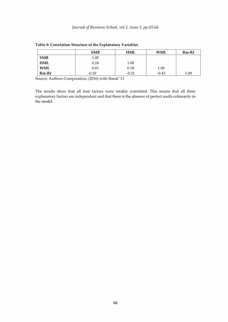
Journal of Business School, vol.1, issue.1, pp.45-‐‑66
66
Table 8: Correlation Structure of the Explanatory Variables
SMB HML WML Rm-‐‑Rf SMB HML WML Rm-‐‑Rf
1.00 0.24 0.01
-‐‑0.10
1.00 0.18 -‐‑0.31
1.00 -‐‑0.43
1.00 Source: Authors Computation, (2016) with StataC 13 The results show that all four factors were weakly correlated. This means that all three explanatory factors are independent and that there is the absence of perfect multi-‐‑colinearity in the model.