Joint PP and PS AVA seismic inversion usingexact Zoeppritz equations

Jun Lu1, Zhen Yang1, Yun Wang2, and Ying Shi1

ABSTRACT

The Zoeppritz equations describe the relationship betweenseismic properties that are useful for the interpretation of lithol-ogy and fluid properties. Various approximations to the Zoeppritzequations are often used in linear amplitude variation with offsetand amplitude variation with angle inversions, assuming low-contrast boundaries. These approximations restrict the inversionmethod to not-too-large-angle cases and reduce the inversionaccuracy. Therefore, it is necessary to develop joint PP and PSprestack inversion methods using the exact Zoeppritz equations.We have developed a method for nonlinear joint prestack inver-sion using the exact Zoeppritz equations. We established an ob-jective function to combine PP and PS information based on a

least-squares approach, and we used the Taylor expansion methodto derive a model updating formula for the inversion. We alsoused a mean shift method to improve the accuracy of inversionresults. We validated our inversion using synthetic and field seis-mic data. The model for calculating synthetic data containedhigh-contrast interfaces to match the reservoir layers, which in-cluded, for example, coal seams and unconsolidated sandstone.The outputs of the inversion were the elastic parameters (P- andS-wave velocities, as well as density), rather than the changes inelastic parameters. We found that the nonlinear joint prestack in-version achieved more accurate results than the linear joint pre-stack inversion, regardless of incidence angle size. Furthermore,if the prestack data were of high enough quality, it was possible toidentify thin layers from the inversion result.

INTRODUCTION

The technique of amplitude variation with offset (AVO), or am-plitude variation with incidence angle (AVA), has been used to pre-dict lithology and fluid properties for decades (Ostrander, 1982;1984; Sun et al., 2008). The Zoeppritz equations describe the rela-tionship between reflection and transmission coefficients for a givenincidence angle, and elastic media properties (P- and S-wave veloc-ities, as well as density). Because the Zoeppritz equations arenonlinear functions with respect to these properties, many approx-imations have been made to linearize them to simplify calculations.These approximations have played a key role in the estimation ofelastic parameters by AVO/AVA inversions.P-wave AVO/AVA methods have been developed over decades

and remarkable advances have been achieved. Since Ostrander(1982) proposes an AVO method to extract lithology and pore-fluid

information from prestack seismic amplitudes, AVO has been usedwith varying rates of success (Larsen, 1999). Shuey (1985) devel-ops a gradient-intercept method that estimates zero-offset reflectiv-ity and changes in Poisson’s ratio. Smith and Gidlow (1987)estimate rock properties by a weighted stacking method usingtime- and offset-variant weights to PP data samples before stacking.Roberts et al. (2002) use an AVO method to enhance the reservoircharacterization based on the long-offset seismic data. However, afew years of experience in P-mode AVO observation leads to resultsthat are sometimes too ambiguous to interpret (Jin, 1999).Compared with P-wave approaches alone, joint AVO inversion of

PP and PS data can provide better estimates of elastic parameters(Kurt, 2007); however, most AVO studies use two-parameter inver-sion methods because three-parameter inversions are often plaguedby numerical instability (Ursenbach and Stewart, 2008). Stewart(1990) extends the weighted stacking method to invert PP- and

Manuscript received by the Editor 15 October 2014; revised manuscript received 23 May 2015; published online 29 July 2015.1China University of Geosciences, Key Laboratory of Marine Reservoir Evolution and Hydrocarbon Accumulation Mechanism, Ministry of Education,

Beijing, China. E-mail: lujun615@163.com; zhendexiangzi@yahoo.com; quartzsy@163.com.2Chinese Academy of Sciences, Institute of Geochemistry, Guiyang, China. E-mail: yunwang@mail.iggcas.ac.cn.© The Authors. Published by the Society of Exploration Geophysicists. All article content, except where otherwise noted (including republished material), is

licensed under a Creative Commons Attribution 4.0 Unported License (CC BY). See http://creativecommons.org/licenses/by/4.0/. Distribution or reproduction ofthis work in whole or in part commercially or noncommercially requires full attribution of the original publication, including its digital object identifier (DOI).

R239

GEOPHYSICS, VOL. 80, NO. 5 (SEPTEMBER-OCTOBER 2015); P. R239–R250, 20 FIGS., 1 TABLE.10.1190/GEO2014-0490.1

Dow

nloa

ded

06/0

9/16

to 6

0.24

7.51

.46.

Red

istr

ibut

ion

subj

ect t

o SE

G li

cens

e or

cop

yrig

ht; s

ee T

erm

s of

Use

at h

ttp://

libra

ry.s

eg.o

rg/

PS-waves jointly for rock property estimations. Fatti et al. (1994)improve the weighted stacking method to directly estimate frac-tional P and S impedance, but their method requires the angle ofincidence less than 35° and P- to S-wave velocity ratios between1.5 and 2.0. Xu and Bancroft (1997) express the P-P and P-S re-flection coefficient equations with the elastic parameters (λ and μ, orκ and μ) and extract these parameters directly without conversionfrom velocity. Larsen (1999) presents a method to invert PP andPS AVO gathers simultaneously to estimate P and S impedance.Ursenbach and Stewart (2008) derive inversion error expressionsfor various two-parameter inversion methods, and obtain flexibleconversion formulas that can convert the results of any two-param-eter method to those of any other two-parameter method. However,two-parameter methods lose important density information, anAVO attribute that is useful for inferring fluid saturation (Downton,2005).For this reason, a significant amount of work has been done on

elastic three-parameter estimations. Jin (1999) presents a real dataexample of a joint P- and S-wave AVO analysis that estimates elas-tic parameters for reservoir characterization, and proposes that S-wave data gave the opportunity to estimate S-wave velocity anddensity variations. Jin et al. (2000) use singular-value decomposi-tion (SVD) to stabilize the linearized PS system of equations, andthey obtain good results for synthetic and field data. Buland andOmre (2003) develop a new linearized AVO inversion method usingBayesian techniques to obtain P- and S-wave velocities, as well asdensity distributions. Mahmoudian and Margrave (2004) formulatethe joint AVO inversion using SVD methods to obtain P- and S-impedance contrasts, as well as density contrast. Three-parameterinversion methods are also investigated by Downton and Lines(2004), Mahmoudian (2006), and Veire and Landrø (2006), butall these studies solve approximations of the Zoeppritz equations.The underlying assumption of these approximations is that the in-cidence angle is not too large and the contrast in elastic parametersis weak (Aki and Richards, 1980; Zhi et al., 2013); however, theseapproximations affect the accuracy of calculations, and they are par-ticularly unsuitable in the case of a strong contrast between layers,such as that between a coal seam and unconsolidated sandstone.Therefore, a joint AVO/AVA inversion method using exact Zoep-pritz equations would represent a more robust method of estimatingelastic parameters using multicomponent seismic data (Zhi etal., 2013).Some attempts at solving the exact Zoeppritz equations have

been made. For example, Tigrek et al. (2005) develop a methodto relate the offset-dependent seismic reflections to the local stressdistributions, and obtain accurate result by joint AVA analysis basedon the full-Zoeppritz equations. Wang et al. (2011) estimate modelparameters with the exact Zoeppritz equations using a generalizedlinear inversion. Zhu and McMechan (2012) propose a new algo-rithm using the exact Zoeppritz equations to obtain four indepen-dent parameters (a density ratio and three velocity ratios) for PPreflections. Zhi et al. (2013) rewrite the exact Zoeppritz equationsas a function of four independent parameters to invert PP- and PS-waves jointly; however, these inversion results are elastic parametercontrasts, not the elastic properties themselves.In this paper, we present a method of joint AVA inversion using

the exact Zoeppritz equations for PP and PS seismic data. The in-verted parameters are P- and S-wave velocities, as well as density.Using a least-squares approach, we establish a joint objective func-

tion that is used to judge whether the difference between simulatedand observed records is small enough to end the inversion. To applythe method to field data, some preprocessing is needed, such as true-amplitude processing of the PP and PS data and compression of thePS AVA data set to the PP traveltime domain. The performance ofthe proposed method is determined by comparison with the syn-thetic and field seismic data. We also compare the results of thelinear and nonlinear joint AVA inversion methods.

METHODOLOGY

For a welded solid-solid interface between two homogeneousisotropic elastic half-spaces, the P- and S-wave velocities, as wellas the density of the upper half-space are denoted by α1, β1, and ρ1,respectively; and in the lower half-space by α2, β2, and ρ2. When aplane P-wave propagates across the interface with a nonzero inci-dence angle, reflecting and transmitting P- and S-waves are gener-ated, and can be described by the Zoeppritz equations. Accuratesolutions of the Zoeppritz equations for PP- and PS-wave reflectioncoefficients were given by Aki and Richards (1980) as

RPP ¼��

bcos i1α1

− ccos i2α2

�F

−�aþ d

cos i1α1

cos j2β2

�Hp2

�∕D (1)

and

RPS ¼ −2cos i1α1

�abþ cd

cos i2α2

cos j2β2

�pα1∕ðβ1DÞ; (2)

where

8>><>>:

a ¼ ρ2ð1 − 2β22p2Þ − ρ1ð1 − 2β21p

2Þ;b ¼ ρ2ð1 − 2β22p

2Þ þ 2ρ1β21p

2;c ¼ ρ1ð1 − 2β21p

2Þ þ 2ρ2β22p

2;d ¼ 2ðρ2β22 − ρ1β

21Þ

(3)

and

8>>>>>><>>>>>>:

E ¼ b cos i1α1

þ c cos i2α2

;

F ¼ b cos j1β1

þ c cos j2β2

;

G ¼ a − d cos i1α1

cos j2β2

;

H ¼ a − d cos i2α2

cos j1β1

;D ¼ EF þGHp2.

(4)

Additionally,i1 and i2 are the P-wave angles of incidence andtransmission across the interface, respectively, and j1 and j2 denotethe S-wave angles of incidence and transmission, respectively.The value p is the ray parameter, which is constant for all layers,and p ¼ sin i1∕α1 ¼ sin i2∕α2 ¼ sin j1∕β1 ¼ sin j2∕β2 (Aki andRichards, 1980).Our goal is to invert the elastic parameter vector using PP and PS

AVA data sets jointly, based on the exact PP- and PS-wave reflec-tion coefficients. According to a least-squares approach, the jointobjective function, Q, for nonlinear inversion is

QðVÞ ¼ wkSPP − DPPk2 þ ð1 − wÞkSPS − DPSk2; (5)

R240 Lu et al.

Dow

nloa

ded

06/0

9/16

to 6

0.24

7.51

.46.

Red

istr

ibut

ion

subj

ect t

o SE

G li

cens

e or

cop

yrig

ht; s

ee T

erm

s of

Use

at h

ttp://

libra

ry.s

eg.o

rg/

where V ¼ ðα; β; ρÞ, and it denotes the model parameter vector forthe target time window. Here, DPP and DPS are the real PP and PSAVA data sets, respectively. The SPP and SPS are the synthetic PPand PS AVA data sets for the given model parameter vector V. And

�SPP ¼ WPP � RPP;SPS ¼ WPS � RPS;

(6)

where WPP and WPS denote the PP- and PS-wavelets, respectively,at a given incidence angle. Here, RPP and RPS are derived from theexact solutions of the Zoeppritz equations shown in equations 1 and2. In the following model test, we also use Aki and Richards’ (1980)approximations to the Zoeppritz equations for RPP and RPS to com-pare the results of linear and nonlinear inversions. The weight factorw ranging from 0 to 1 is used to qualify the two data sets. When thePP data set is of a higher quality than the PS data set, w is larger than0.5; if only the PP data are used during the inversion, then w is set to1. In the model tests presented here, the quality of the two data setsis assumed to be equal, so w is set to 0.5.Given a forward model parameter vector, RPP or RPS can be ex-

panded into a truncated Taylor series expansion around V ¼ V0,whereV0 is the initial parameter vector. This expanded Taylor serieshas the form

RPXðV0 þ ΔVÞ ¼ RPX0ðV0Þ þGðVÞΔV: (7)

Here, X denotes P or S, ΔV ¼ ðΔα;Δβ;ΔρÞ, and Δα, Δβ, andΔρ are the desired updates of the current model vectorV0. TheRPX0

is the PP or PS reflection coefficient vector at a different incidenceangle to that of the initial model. The Jacobian matrix G has theform

G ¼

2666664

∂R1

∂V1

∂R1

∂V2· · · ∂R1

∂Vn∂R2

∂V1

∂R2

∂V2· · · ∂R2

∂Vn

..

. ... . .

. ...

∂Rn∂V1

∂Rn∂V2

· · · ∂Rn∂Vn

3777775; (8)

where the subscripts 1 to n denote different target time sample se-quences.Substituting equations 6 and 7 into equation 5 gives

QðVÞ ¼ wkWPP � ðRPP þGPPΔVÞ − DPPk2þ ð1 − wÞkWPS � ðRPS þGPSΔVÞ − DPSk2: (9)

Using a least-squares approach, we then have

∂QðVÞ∂ΔV

¼ w½ðWPP � RPP − DPPÞTðWPP �GPPÞþ ðWPP �GPPΔVÞTðWPP �GPPÞ�þ ð1 − wÞ½ðWPS � RPS − DPSÞTðWPS �GPSÞþ ðWPS �GPSΔVÞTðWPS �GPSÞ�

¼ 0; (10)

giving

ΔV ¼ ½wHTPPHPP þ ð1 − wÞHT

PSHPS�−1· ½wHT

PPEPP þ ð1 − wÞHTPSEPS�: (11)

Here, HPX ¼ WPX �GPX and EPX ¼ DPX −WPX � RPX0. Thevalue EPX is the residual matrix between the real seismic dataand the forward model response for the initial elastic parameters.We use ΔV to update the initial model parameter vector V0 itera-tively until the joint objective functionQ reaches a minimum. Equa-tion 11 is an unstable solution. Therefore, we use the Levenberg-Marquardt method (Levenberg, 1944; Marquardt, 1963) to solve thesingular nonlinear equations, and we modify equation 11 to

ΔV ¼ ½wHTPPHPP þ ð1 − wÞHT

PSHPS þ ηI�−1· ½wHT

PPEPP þ ð1 − wÞHTPSEPS þ ηI�; (12)

where η is a Lagrange multiplier and I is an identity matrix.To ensure the inversion accuracy, a mean shift method was ap-

plied to constrain the inversion result. After some iterations, we de-rive an elastic parameter model that is close to the prior model byextrapolating from the well model along horizons. If the ratio be-tween the mean value of the inverse elastic parameters and the priormodel parameters is large, then this ratio is used to scale the inversemodel to improve its proximity to the prior model. Mean shift canbe considered as the low-frequency compensation of the model.To apply the above method to field PP- and PS-waves, special

processing techniques are needed for: (1) P- and S-mode separationfrom vertical and horizontal components, (2) PS to PP time align-ment, and (3) wavelet extraction at different incidence angles.

P- and S-mode separation from vertical and horizontalcomponents

In multicomponent seismology, multiple field shot records aremeasured (shown as “mode leakage”), allowing for potentialcross-contamination of P-wave energy in the horizontal componentand S-wave energy in the vertical component. Suppressing modeleakage by P- and S-wave separation is an important step in prestackmulticomponent seismic data processing. For this study, we appliedthe method introduced by Lu et al. (2012) to separate differentwave modes.

PS to PP time alignment

Owing to the use of a joint objective function during the inver-sion, the PS time should be aligned with PP time by compressing PStime. To do this, the PS events need to match to the PP events fromthe same geologic strata with the help of well data and syntheticrecords. An instantaneous gamma volume γi can be derived afteraccurate horizon matching:

γi ¼ TPPi∕TPSj; (13)

where TPPi denotes the PP reflection time for sample i, and TPSi

denotes the PS reflection time for sample j. Samples i and j arefrom the same depth. We use γi to compress the PS AVA data setto the PP time-domain sample by sample.

Joint PP and PS AVA seismic inversion R241

Dow

nloa

ded

06/0

9/16

to 6

0.24

7.51

.46.

Red

istr

ibut

ion

subj

ect t

o SE

G li

cens

e or

cop

yrig

ht; s

ee T

erm

s of

Use

at h

ttp://

libra

ry.s

eg.o

rg/

Wavelet extraction at different incidence angles

The inversion output is the elastic parameter vector, rather thanthe change in an elastic parameter, so wavelets must be defined.Some prestack processing procedures, such as Q-compensation,event stretching, and compression, may lead to the changes ofPP- and PS-wavelets at each incidence angle. Wavelets shouldtherefore be extracted from PP and PS data sets separately for thejoint inversion, at the total incidence angle. Most other wavelet-extraction methods for PP-waves are suitable for our inversionmethod. For example, a statistical method of kurtosis maximizationby constant-phase rotation developed by Baan (2008) can produce astationary, constant-phase wavelet (Jonathan and Baan, 2011).

SYNTHETIC DATA TEST

To test our method against synthetic data, we used a five-layer 1Dmodel with high-contrast interfaces (shown in Table 1), and syn-thetic PP and PS AVA data sets within critical angles, as shownin Figure 1. To correlate the PP and PS events, we change the polar-ities of PS-waves to match those of PP-waves when they are oppo-site. These data sets are generated with a 1-ms sample rate throughconvolution of the reflectivity derived from the exact Zoeppritzequation and Ricker wavelets with dominant frequencies of40 Hz for PP-waves and 30 Hz for PS-waves in PP time, respec-

tively. Interference, such as noise and multiples, was not taken intoaccount in the forward modeling. Two different inversion modelswere tested: (1) the nonlinear joint PP and PS AVA inversion basedon exact PP and PS reflection coefficients presented above (NJI)

Table 1. Theoretical model parameters.

α (m∕s) β (m∕s) ρ (g∕cm3) Thickness (m)

2800 933 2.28 100

3200 1600 2.35 100

2000 1333 2.0 3

3300 1650 2.35 80

3400 1700 2.52 390

Figure 1. Synthetic (a) PP and (b) PS seismograms in the PP timedomain without noise.

a) b)

300

250

200

150

100

50

0

Tim

e (m

s)

300

0.5 1.0 1.5 2.0(km/s or g/cm3)

2.5 3.0 3.5 4.0 0.5 1.0 1.5 2.0(km/s or g/cm3)

2.5 3.0 3.5 4.0

250

200

150

100

50

0

Tim

e (m

s)

Figure 2. (a) Linear initial model and (b) noise-added initial modelgenerated from the actual model plus 5% random noise. The redcurve is the S-wave initial model, the blue curve is the density initialmodel, and the black curve is the P-wave initial model. These mod-els are used to test the influence of the initial model on the inversionresult.

300

250

200

150

100

50

0a) b)

Tim

e (m

s)

300

250

200

150

100

50

0

Tim

e (m

s)

2.0 2.4 2.8 3.2 3.6 4.0 4.4P-wave velocity (km/s)

2.0 2.4 2.8 3.2 3.6 4.0 4.4P-wave velocity (km/s)

Figure 3. P-wave velocity inversion results inverted by (a) NJI and(b) LJI using the linear initial model. The blue curve is the initialmodel, the red curve is the inverse result, and the black curve is thetrue model.

R242 Lu et al.

Dow

nloa

ded

06/0

9/16

to 6

0.24

7.51

.46.

Red

istr

ibut

ion

subj

ect t

o SE

G li

cens

e or

cop

yrig

ht; s

ee T

erm

s of

Use

at h

ttp://

libra

ry.s

eg.o

rg/

and (2) a linear joint PP and PS AVA inversion based on Aki andRichards’ (1980) approximate PP and PS reflection coefficients(LJI). The linear single PP AVA inversion based on Aki and Ri-chards’ (1980) approximate PP reflection coefficients (LSI) is alsotested. But the results of LSI are closed to that of LJI, so we just

show the results of NJI and LJI for comparison. For joint inversions,the weight factor w was set to 0.5 (i.e., the two data sets wereassumed to have equal quality). For nonlinear and linear in-versions, the Jacobian matrix G was constructed using equation 8,although the nonlinear inversion used the exact Zoeppritz

300

0.8 1.2 1.6 2.0 2.4

250

200

150

100

50

0a)

Tim

e (m

s)

b)

300

250

200

150

100

50

0

Tim

e (m

s)

S-wave velocity (km/s)0.8 1.2 1.6 2.0 2.4

S-wave velocity (km/s)

Figure 4. S-wave velocity inversion results inverted by (a) NJI and(b) LJI using the linear initial model. The blue curve is the initialmodel, the red curve is the inverse result, and the black curve is thetrue model.

300

250

200

150

100

50

0a)

Tim

e (m

s)

b)

300

250

200

150

100

50

0

Tim

e (m

s)

1.6 1.8 2.0 2.2 2.4 2.6 2.8 3.0Density (g/cm3)

1.6 1.8 2.0 2.2 2.4 2.6 2.8 3.0Density (g/cm3)

Figure 5. Density inversion results inverted by (a) NJI and (b) LJIusing the linear initial model. The blue curve is the initial model, thered curve is the inverse result, and the black curve is the true model.

300

0.8 1.2 1.6 2.0 2.4

250

200

150

100

50

0a)

Tim

e (m

s)

300

250

200

150

100

50

0b)

Tim

e (m

s)

S-wave velocity (km/s)0.8 1.2 1.6 2.0 2.4

S-wave velocity (km/s)

Figure 7. S-wave velocity inversion results inverted by (a) NJI and(b) LJI using the 5% noise-added initial model. The blue curve is theinitial model, the red curve is the inverse result, and the black curveis the true model.

300

250

200

150

100

50

0a)

Tim

e (m

s)

b)

300

250

200

150

100

50

0

Tim

e (m

s)

2.0 2.4 2.8 3.2 3.6 4.0 4.4 4.8P-wave velocity (km/s)

2.0 2.4 2.8 3.2 3.6 4.0 4.4 4.8P-wave velocity (km/s)

Figure 6. P-wave velocity inversion results inverted by (a) NJI and(b) LJI using the 5% noise-added initial model. The blue curve is theinitial model, the red curve is the inverse result, and the black curveis the true model.

Joint PP and PS AVA seismic inversion R243

Dow

nloa

ded

06/0

9/16

to 6

0.24

7.51

.46.

Red

istr

ibut

ion

subj

ect t

o SE

G li

cens

e or

cop

yrig

ht; s

ee T

erm

s of

Use

at h

ttp://

libra

ry.s

eg.o

rg/

solutions, whereas the linear inversion used Aki and Richards’(1980) approximations.A linear model and a noise-added model (shown in Figure 2)

were used to test the sensitivity of our inversion method to thechoice of the initial model. The inversion results (without any meanshift corrections) with the linear initial model using the (a) NJI and(b) LJI methods are shown in Figures 3–5 for P- and S-wave veloc-ities, as well as density, respectively. Although the stratigraphic con-trast cannot be seen on the plot of the linear initial model(Figure 2a), NJI (Figures 3a, 4a, and 5a) produces a good result,showing a thin layer that exactly conforms to the true model. Incontrast, LJI (Figures 3b, 4b, and 5b) produce poor results because

the true model has strong contrast parameters and a small stratumthickness. Figures 6–8 display inversion results for the noise-addedinitial model, and show that NJI (Figures 6a, 7a, and 8a) producesstable results compared with LJI (Figures 6b, 7b, and 8b).Figures 3–8 show that inversion methods based on exact Zoep-

pritz solutions pick up the thin low-impedance layer in the truemodel. The inverted P- and S-wave velocities are closer to the truemodel values than are the inverted densities because density exhib-its little sensitivity to amplitudes and the use of angle-limited AVAdata may have affected its stability (Lines, 1998; Alemie and Sac-chi, 2011; Du and Yan, 2013). However, for the model described inTable 1, larger incidence angles will cause critical reflectivity. Amean shift method, which is used to constrain the inversion pro-cedure to improve the inversion accuracy, was applied to the NJImodel results when the initial model was linear. As shown in Fig-ure 9, the inversion constrained by the mean shift method is virtu-ally identical to the true model.

300

1.2 1.6 2.0 2.4 2.8 3.2 3.6

250

200

150

100

50

0a)

Tim

e (m

s)

b)

300

250

200

150

100

50

0

Tim

e (m

s)

Density (g/cm3)

1.2 1.6 2.0 2.4 2.8 3.2 3.6Density (g/cm3)

Figure 8. Density inversion results inverted by (a) NJI and (b) LJIusing the 5% noise-added initial model. The blue curve is the initialmodel, the red curve is the inverse result, and the black curve is thetrue model.

300

2.0 2.4 2.8 3.2 3.6 4.0 4.4

250

200

150

100

50

0a)

Tim

e (m

s)

300

0.8 1.2 1.6 2.0 2.4 1.6 1.8 2.0 2.2 2.4 2.6 2.8 3.0

250

200

150

100

50

0b)

Tim

e (m

s)

300

250

200

150

100

50

0c)

Tim

e (m

s)

P-wave velocity (km/s) S-wave velocity (km/s) Density (g/cm3)

Figure 9. Mean shift in (a) P-wave velocity, (b) S-wave velocity, and (c) density inverted by the NJImethod from the linear initial model. The bluecurve is the initial model, and the red curve isthe inverse result, which is coincident with the truemodel.

Figure 10. Synthetic (a) PP and (b) PS AVA records with a noiselevel of 16%.

R244 Lu et al.

Dow

nloa

ded

06/0

9/16

to 6

0.24

7.51

.46.

Red

istr

ibut

ion

subj

ect t

o SE

G li

cens

e or

cop

yrig

ht; s

ee T

erm

s of

Use

at h

ttp://

libra

ry.s

eg.o

rg/

300

250

200

150

100

50

0a)

Tim

e (m

s)

300

1.5 2.0 2.5 3.0 3.5 4.0 4.5 0.5 1.0 1.5 2.0 2.5 1.6 2.0 2.4 2.8 3.2

250

200

150

100

50

0b)

Tim

e (m

s)

300

250

200

150

100

50

0c)

Tim

e (m

s)

P-wave velocity (km/s) S-wave velocity (km/s) Density (g/cm3)

Figure 11. Inversion results by NJI method: (a) P-wave velocity, (b) S-wave velocity, and (c) density.The red curve is the NJI inversion result with 1%noise added to the synthetic PP and PS AVA re-cords, and the black curve is the true model.

300

250

200

150

100

50

0a)

Tim

e (m

s)

300

250

200

150

100

50

0b)

Tim

e (m

s)

300

250

200

150

100

50

0c)

Tim

e (m

s)

1.5 2.0 2.5 3.0 3.5 4.0 4.5P-wave velocity (km/s)

0.5 1.0 1.5 2.0 2.5S-wave velocity (km/s)

1.6 2.0 2.4 2.8 3.2Density (g/cm3)

Figure 12. The trend lines calculated by the low-pass filtered NJI results: (a) P-wave velocity, (b) S-wave velocity, and (c) density. The red curve is theNJI result, the purple curve is the trend line, andthe blue line marks the turning point in the trendline.

300

250

200

150

100

50

0a)

Tim

e (m

s)

300

250

200

150

100

50

0b)

Tim

e (m

s)

300

250

200

150

100

50

0c)

Tim

e (m

s)

1.5 2.0 2.5 3.0 3.5 4.0 4.5

P-wave velocity (km/s)0.5 1.0 1.5 2.0 2.5S-wave velocity (km/s)

1.6 2.0 2.4 2.8 3.2Density (g/cm3)

Figure 13. Inversion results by NJI method: (a) P-wave velocity, (b) S-wave velocity, and (c) density,where the red curve represents the NJI inversionresult shown in Figure 11 smoothed by piecewisesmoothing algorithm, and the black curve is thetrue model.

Joint PP and PS AVA seismic inversion R245

Dow

nloa

ded

06/0

9/16

to 6

0.24

7.51

.46.

Red

istr

ibut

ion

subj

ect t

o SE

G li

cens

e or

cop

yrig

ht; s

ee T

erm

s of

Use

at h

ttp://

libra

ry.s

eg.o

rg/

Any acquired seismic record will contain a certain amount ofnoise, and inversion accuracy is highly dependent upon this noiselevel. To assess the sensitivity of our method to noise, we add ran-dom noise with different weights to the synthetic PP and PS seismo-grams separately. As shown in Figure 10, a noise level of 16% wasgenerated randomly in the time domain, with noise values distrib-uted normally around the synthetic signal.Figure 11 shows the NJI results overlaid with the true values

when 1% noise was added to the AVA records. The inversion resultis close to the true model, including the thin layer with large elastic

contrasts, even though it is noisy. To suppress the noise for the in-version, we smoothed the inversion model values using a piecewisesmoothing algorithm to obtain an improved inversion result. First,as shown in Figure 12, a low-pass filter is applied to get the trendline of the inversion results. Second, the turning points are distin-guished from the trend line for dividing the trend line into severalsegments. Finally, the inversion result is smoothed in each segment.The smoothing results at the noise level of 1% are shown in Fig-ure 13, and the results reveal the thin layer more effectively. Thesmoothing method also produces stable NJI results when a noise

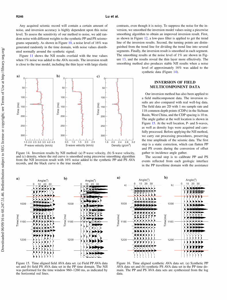
level of approximately 16% was added to thesynthetic data (Figure 14).

INVERSION OF FIELDMULTICOMPONENT DATA

Our inversion method has also been applied toa field multicomponent data. The inversion re-sults are also compared with real well-log data.The field data are 2D with 1 ms sample rate and118 common depth points (CDPs) in the SichuanBasin, West China, and the CDP spacing is 10 m.The angle gather at the well location is shown inFigure 15. At the well location, P- and S-waves,as well as density logs were acquired and care-fully processed. Before applying the NJI method,we carry out processing procedures, preservingthe true amplitude of the seismic data. The firststep is a static correction, which can flatten PPand PS events during the conversion of offsetgather to incidence angle gather.The second step is to calibrate PP and PS

events reflected from each geologic interfacein the PP traveltime domain with the assistance

Figure 15. Time aligned field AVA data set. (a) Field PP AVA dataset and (b) field PS AVA data set in the PP time domain. The NJIwas performed for the time window 960–1260 ms, as indicated bythe horizontal red lines.

Figure 16. Time aligned synthetic AVA data set. (a) Synthetic PPAVA data set and (b) synthetic PS AVA data set in the PP time do-main. The PP and PS AVA data sets are synthesized from the logdata.

300

250

200

150

100

50

0a)

Tim

e (m

s)

300

250

200

150

100

50

0b)

Tim

e (m

s)

300

250

200

150

100

50

0c)

Tim

e (m

s)

1.5 2.0 2.5 3.0 3.5 4.0 4.5P-wave velocity (km/s)

0.5 1.0 1.5 2.0 2.5S-wave velocity (km/s)

1.6 2.0 2.4 2.8 3.2Density (g/cm3)

Figure 14. Inversion results by NJI method: (a) P-wave velocity, (b) S-wave velocity,and (c) density, where the red curve is smoothed using piecewise smoothing algorithmfrom the NJI inversion result with 16% noise added to the synthetic PP and PS AVArecords, and the black curve is the true model.

R246 Lu et al.

Dow

nloa

ded

06/0

9/16

to 6

0.24

7.51

.46.

Red

istr

ibut

ion

subj

ect t

o SE

G li

cens

e or

cop

yrig

ht; s

ee T

erm

s of

Use

at h

ttp://

libra

ry.s

eg.o

rg/

of synthetic seismograms calculated from well logs (Figure 16).During this procedure, PP and PS time-to-depth log conversionsare calculated and used for PS data set compression. Compared with

Figure 16, it can be seen that the PP and PS seismograms in the PPtraveltime domain shown in Figure 15 correlate well with syntheticseismograms after event correlation. Though the PS-field AVA data

Figure 17. Wavelet extracted from time aligneddata. (a) Wavelet of the PP AVA data set and(b) wavelet of the PS AVA data set, after com-pressing to the PP traveltime domain.

Figure 18. Inverted sections: (a) P-wave velocityby NJI method, (b) P-wave velocity by LJImethod, (c) S-wave velocity by NJI method,and (d) S-wave velocity by LJI method. The blackcurve is the well log.

Joint PP and PS AVA seismic inversion R247

Dow

nloa

ded

06/0

9/16

to 6

0.24

7.51

.46.

Red

istr

ibut

ion

subj

ect t

o SE

G li

cens

e or

cop

yrig

ht; s

ee T

erm

s of

Use

at h

ttp://

libra

ry.s

eg.o

rg/

set is formed from the raw data with a worse signal-to-noise ratio, itscorrelation coefficient with the synthetic data set is up to 0.65 aftercareful processing. The correlation coefficient between the actualand synthetic PPAVA data sets is 0.76. So, we set the weight factorw in equation 5 to 0.5 because the two correlation coefficientsare close.The final step is to extract wavelets of PP and PS AVA data sets

separately. We extract the statistical wavelets over the entire inci-dence angle range separately after event correlation. Figure 17shows that both wavelets are zero phase and have similar mainfrequencies but differing side lobes.The inverted sections are shown in Figures 18 and 19, where the

green and red colors represent the shale and the sand contents of thelayer, separately, which are calibrated by well logs. It shows that wecan distinguish more thin layers from the sections inverted by theNJI method than by the LJI method. Compared with the otherparameters, the velocity-ratio section (Figure 19c) inverted byNJI method shows obviously higher resolution. The near-wellinversion results are extracted from the sections and shown in

Figure 20. We can see that good calibration at the well positionmade the near-well inversion results closely match the well logs.Though the inversion results have lower frequency content than thewell logs because of the limited frequency of the wavelet, NJI canproduce a high-resolution result, which is beneficial to the recog-nition of thin layer.

DISCUSSION

Our NJI inversion method requires careful data processing. Sometrue-amplitude processing techniques are mentioned in the above.Incidence angle is an important factor, which will affect the inver-sion result seriously. In cases of complicated structures, we can usea ray-tracing method to calculate the raypath at the target interfaceand derive the accurate incidence angle, which is out of the scope ofthis paper.Noise attenuation is also quite important. Noise in the AVA data

set will increase the uncertainty in the inversion result, but we candecrease the weight factor of the uncertain component to reduce the

Figure 19. Inverted sections: (a) density by NJImethod, (b) density by LJI method, (c) P- to S-wave velocity ratios by NJI method, and (d) P-to S-wave velocity ratios by LJI method. The αto β ratios are derived from the inverted P- andS-wave velocities. The black curve is the well log.

R248 Lu et al.

Dow

nloa

ded

06/0

9/16

to 6

0.24

7.51

.46.

Red

istr

ibut

ion

subj

ect t

o SE

G li

cens

e or

cop

yrig

ht; s

ee T

erm

s of

Use

at h

ttp://

libra

ry.s

eg.o

rg/

noise effect. However, to distinguish thin layer information from theinversion result, we do not want the data to be filtered too hard be-fore inversion.Our inversion method does not consider anisotropy, so the neg-

ative effects of elastic parameter anisotropy on multicomponentseismic data must be eliminated. For vertical transverse isotropy(VTI) anisotropy, we can consider using a nonhyperbolic moveoutcorrection technique to obtain large-angle data. Furthermore, in thecase of horizontal transverse isotropy (HTI) anisotropy, phase error,induced by S-wave splitting, must be compensated in prestackprocessing. Many fast and slow S-wave separation methods canbe used to compensate such phase error.For thin layer models, it is hard to get the interface reflections

only because the reflections from the top and bottom interfacesof the thin layer will interfere together and cannot be separated.Moreover, interbed multiples and converted waves are hard to sup-press, also they will influence the amplitude and phase of the targetreflection. Therefore, to pick up the thin layer from the inversionresult of field data, it is necessary to deduce the reflection coefficientformula of the thin layer.Event matching is crucial to joint PP and PS AVA inversion. The

PS wavelet will change with time when compressed to PP time be-cause of the time-variant compression ratio. Therefore, the PSwavelet should be extracted from the compressed data, and the timewindow chosen for inversion should be short enough to retain sta-bility of the wavelet. It is necessary for us to explore a more effec-tive method to improve event matching and PS-wave extraction infuture work.

CONCLUSIONS

We have developed a joint AVA inversion method (NJI) using theexact Zoeppritz equations for PP and PS seismic data, and we have

tested the model for synthetic and field seismic data. When dealingwith high-contrast interfaces, inversion methods based on approx-imations to the Zoeppritz equations are insufficient, but our NJImethod can achieve significantly better results.The synthetic data example shows that it is possible to reveal a

thin layer even with a linear initial model or with small amount ofnoise. The inverted elastic properties show a high level of randomperturbation when a large amount of noise added to the syntheticdata; however, the thin layer can still be revealed after a piecewisesmoothing operation applied. Our NJI method is suitable for largerincidence angles, so velocity analysis and NMO corrections forlarge offset data must be applied before AVA gather formation;however, even in small incidence angle cases, the NJI method offersan advantage over approximation methods because it uses fewertheoretical assumptions. Also, the methodology requires noise sup-pression in AVA gathers, even though stable results can be achievedif the noise level is small.For field data, our NJI method proved helpful in geologic layer

interpretation, even though the PP- and PS-wavelets were narrow.We anticipate that our NJI method would be especially useful inpredicting lithology and fluid properties in fields with thin andlow-impedance layers.

ACKNOWLEDGMENTS

We greatly appreciate the support of PetroChina InnovationFoundation (2011D-5006-0303), the Natural Science Foundationof China (41104084), and the Fundamental Research Funds forthe Central Universities (2-9-2013-093). We are very grateful toZ. Li for sharing the field data. Thanks to T. Chen and an anony-mous reviewer, whose comments and suggestions significantly im-proved the manuscript.

1240

1200

1160

1120

1080

1040

1000

960

Tim

e (m

s)

1240

1200

1160

1120

1080

1040

1000

960

Tim

e (m

s)

1240

1200

1160

1120

1080

1040

1000

960

Tim

e (m

s)

1240

1200

1160

1120

1080

1040

1000

960

Tim

e (m

s)

3.0 3.5 4.0 4.5 5.0 5.5 6.0 2.0 2.4 2.8 3.2 3.6 1.8 2.0 2.2 2.4 2.6 2.8 3.0 1.4 1.6 1.8 2.0S-wave velocity (km/s) P- to S-wave velocity ratioP-wave velocity (km/s) Density (g/cm3)

a) b) c) d)

Figure 20. Near-well inversion results of NJI method (red curves) extracted from the sections: (a) P-wave velocity, (b) S-wave velocity,(c) density, and (d) P- to S-wave velocity ratios, where the black curves are well-log data.

Joint PP and PS AVA seismic inversion R249

Dow

nloa

ded

06/0

9/16

to 6

0.24

7.51

.46.

Red

istr

ibut

ion

subj

ect t

o SE

G li

cens

e or

cop

yrig

ht; s

ee T

erm

s of

Use

at h

ttp://

libra

ry.s

eg.o

rg/

REFERENCES

Aki, K., and P. Richards, 1980, Quantitative seismology: W. H. Freeman &Co.

Alemie, W., and M. D. Sacchi, 2011, High-resolution three-term AVO in-version by means of a Trivariate Cauchy probability distribution: Geo-physics, 76, no. 3, R43–R55, doi: 10.1190/1.3554627.

Buland, A., and H. Omre, 2003, Bayesian linearized AVO inversion: Geo-physics, 68, 185–198, doi: 10.1190/1.1543206.

Downton, J. E., 2005, Seismic parameter estimation from AVO inversion:Ph.D. thesis, University of Calgary.

Downton, J. E., and L. R. Lines, 2004, Three term AVO waveforminversion: 74th Annual International Meeting, SEG, Expanded Abstracts,215–218.

Du, Q. Z., and H. Z. Yan, 2013, PP and PS joint AVO inversion and fluidprediction: Journal of Applied Geophysics, 90, 110–118, doi: 10.1016/j.jappgeo.2013.01.005.

Fatti, J. L., G. C. Smith, P. J. Vail, P. J. Strauss, and P. R. Levitt, 1994, De-tection of gas in sandstone reservoirs using AVO analysis: A 3-D seismiccase history using the geostack technique: Geophysics, 59, 1362–1376,doi: 10.1190/1.1443695.

Jin, S., 1999, Characterizing reservoir by using jointly P- and S-wave AVOanalysis: 69th Annual International Meeting, SEG, Expanded Abstracts,687–690.

Jin, S., G. Cambois, and C. Vuillermoz, 2000, Shear-wave velocity and den-sity estimation from PS-wave AVO analysis: Application to an OBS dataset from the North Sea: Geophysics, 65, 1446–1454, doi: 10.1190/1.1444833.

Jonathan, A. E., and M. Baan, 2011, How reliable is statistical wavelet es-timation?: Geophysics, 76, no. 4, V59–V68, doi: 10.1190/1.3587220.

Kurt, H., 2007, Joint inversion of AVA data for elastic parameters by boot-strapping: Computers & Geosciences, 33, 367–382, doi: 10.1016/j.cageo.2006.08.012.

Larsen, J. A., 1999, AVO inversion by simultaneous P-P and P-S inversion:M.S. thesis, University of Calgary.

Levenberg, K., 1944, A method for the solution of certain non-linear prob-lems in least squares: Quarterly of Applied Mathematics, 2, 164–168.

Lines, L. R., 1998, Density contrast is difficult to determine from AVO:CREWES, Research report 10.

Lu, J., Y. Wang, and C. Yao, 2012, Separating P- and S-waves in an affinecoordinate system: Journal of Geophysics and Engineering, 9, 12–18, doi:10.1088/1742-2132/9/1/002.

Mahmoudian, F., 2006, Linear AVO inversion of multi-component surfaceseismic and VSP data: M.S. thesis, University of Calgary.

Mahmoudian, F., and G. F. Margrave, 2004, Three parameter AVO inversionwith PP and PS data using offset binning: 74th Annual International Meet-ing, SEG, Expanded Abstracts, 240–243.

Marquardt, D. W., 1963, An algorithm for least-squares estimation of non-linear inequalities: Journal of the Society for Industrial and Applied Math-ematics, 11, 431–441, doi: 10.1137/0111030.

Ostrander, W. J., 1982, Plane-wave reflection coefficients for gas sands atnonnormal angles of incidence: 52nd Annual International Meeting, SEG,Expanded Abstracts, 216–218.

Ostrander, W. J., 1984, Plane-wave reflection coefficients for gas sands atnon-normal angles of incidence: Geophysics, 49, 1637–1648, doi: 10.1190/1.1441571.

Roberts, G., D. Went, K. Hawkins, G. Williams, N. Kabir, T. Nash, and D.Whitcombe, 2002, A case study of long-offset acquisition, processingand interpretation over the Harding Field, North Sea: 64th AnnualInternational Conference and Exhibition, EAGE, Extended Abstracts,27–30.

Shuey, R. T., 1985, A simplification of the Zoeppritz equations: Geophysics,50, 609–614, doi: 10.1190/1.1441936.

Smith, G. C., and P. M. Gidlow, 1987, Weighted stacking for rock propertyestimation and detection of gas: Geophysical Prospecting, 35, 993–1014,doi: 10.1111/j.1365-2478.1987.tb00856.x.

Stewart, R. R., 1990, Joint P and P-SV inversion: CREWES, Researchreport 2.

Sun, P. Y., X. L. Lu, Y. P. Li, Y. Y. Yue, and H. F. Chen, 2008, Elastic param-eter AVO approximations and their applications: 78th AnnualInternational Meeting, SEG, Expanded Abstracts, 523–527.

Tigrek, S., E. C. Slob, M. W. P. Dillen, S. A. P. L. Cloetingh, and J. T. Fok-kema, 2005, Linking dynamic elastic parameters to static state of stress:Toward an integrated approach to subsurface stress analysis: Tectonophy-sics, 397, 167–179, doi: 10.1016/j.tecto.2004.10.008.

Ursenbach, C. P., and R. R. Stewart, 2008, Two-term AVO inversion: Equiv-alences and new methods: Geophysics, 73, no. 6, C31–C38, doi: 10.1190/1.2978388.

van der Baan, M., 2008, Time-varying wavelet estimation and deconvolutionby kurtosis maximization: Geophysics, 73, no. 2, V11–V18, doi: 10.1190/1.2831936.

Veire, H. H., and M. Landrø, 2006, Simultaneous inversion of PP and PSseismic data: Geophysics, 71, no. 3, R1–R10, doi: 10.1190/1.2194533.

Wang, Y. M., X. P. Wang, X. J. Meng, and X. M. Niu, 2011, Pre-stack in-version of wide incident angle seismic data: 81st Annual InternationalMeeting, SEG, Expanded Abstracts, 2507–2511.

Xu, Y., and J. C. Bancroft, 1997, Joint AVO analysis of PP and PS seismicdata: CREWES, Research report 9.

Zhi, L. X., S. Q. Chen, and X. Y. Li, 2013, Joint AVO inversion of PP and PSwaves using exact Zoeppritz equation: 83rd Annual International Meet-ing, SEG, Expanded Abstracts, 457–461.

Zhu, X. F., and G. McMechan, 2012, AVO inversion using the Zoeppritzequation for PP reflections: 82nd Annual International Meeting, SEG, Ex-panded Abstracts, doi:10.1190/segam2012-0160.1.

R250 Lu et al.

Dow

nloa

ded

06/0

9/16

to 6

0.24

7.51

.46.

Red

istr

ibut

ion

subj

ect t

o SE

G li

cens

e or

cop

yrig

ht; s

ee T

erm

s of

Use

at h

ttp://

libra

ry.s

eg.o

rg/