joint determination of optimal stratification and sample allocation …€¦ · ·...

Article

Component of Statistics CanadaCatalogue no. 12-001-X Business Survey Methods Division

Joint determination of optimal stratification and sample allocation using genetic algorithm by Marco Ballin and Giulio Barcaroli

January 2014

How to obtain more informationFor information about this product or the wide range of services and data available from Statistics Canada, visit our website, www.statcan.gc.ca.

You can also contact us by

email at [email protected],

telephone, from Monday to Friday, 8:30 a.m. to 4:30 p.m., at the following toll‑free numbers:

• Statistical Information Service 1‑800‑263‑1136• National telecommunications device for the hearing impaired 1‑800‑363‑7629• Fax line 1‑877‑287‑4369

Depository Services Program• Inquiries line 1‑800‑635‑7943• Fax line 1‑800‑565‑7757

To access this productThis product, Catalogue no. 12-001-X, is available free in electronic format. To obtain a single issue, visit our website, www.statcan.gc.ca, and browse by “Key resource” > “Publications.”

Standards of service to the publicStatistics Canada is committed to serving its clients in a prompt, reliable and courteous manner. To this end, Statistics Canada has developed standards of service that its employees observe. To obtain a copy of these service standards, please contact Statistics Canada toll‑free at 1‑800‑263‑1136. The service standards are also published on www.statcan.gc.ca under “About us” > “The agency” > “Providing services to Canadians.”

Published by authority of the Minister responsible for Statistics Canada

© Minister of Industry, 2014.

All rights reserved. Use of this publication is governed by the Statistics Canada Open Licence Agreement (http://www.statcan.gc.ca/reference/licence‑eng.html).

Cette publication est aussi disponible en français.

Standard symbolsThe following symbols are used in Statistics Canada publications:

. not available for any reference period

.. notavailableforaspecificreferenceperiod

... not applicable0 true zero or a value rounded to zero0s value rounded to 0 (zero) where there is a meaningful

distinction between true zero and the value that was rounded

p preliminaryr revisedx suppressedtomeettheconfidentialityrequirementsofthe

Statistics ActE use with cautionF too unreliable to be published* significantlydifferentfromreferencecategory(p<0.05)

Note of appreciationCanada owes the success of its statistical system to a long‑standing partnership between Statistics Canada, the citizens of Canada, its businesses, governments and other institutions. Accurate and timely statistical information could not be produced without their continued co‑operation and goodwill.

http://www.statcan.gc.ca/

mailto:infostats%40statcan.gc.ca?subject=

http://www.statcan.gc.ca

http://www.statcan.gc.ca/

http://www.statcan.gc.ca/reference/licence-eng.html

http://www.statcan.gc.ca/reference/licence-eng.html

Survey Methodology, December 2013 369 Vol. 39, No. 2, pp. 369-393 Statistics Canada, Catalogue No. 12-001-X

1. Marco Ballin and Giulio Barcaroli, Istituto Nazionale di Statistica, via C.Balbo 16 - 00184 Roma (Italy). E-mail: [email protected],

[email protected].

Joint determination of optimal stratification and sample allocation using genetic algorithm

Marco Ballin and Giulio Barcaroli1

Abstract

This paper offers a solution to the problem of finding the optimal stratification of the available population frame, so as to ensure the minimization of the cost of the sample required to satisfy precision constraints on a set of different target estimates. The solution is searched by exploring the universe of all possible stratifications obtainable by cross-classifying the categorical auxiliary variables available in the frame (continuous auxiliary variables can be transformed into categorical ones by means of suitable methods). Therefore, the followed approach is multivariate with respect to both target and auxiliary variables. The proposed algorithm is based on a non deterministic evolutionary approach, making use of the genetic algorithm paradigm. The key feature of the algorithm is in considering each possible stratification as an individual subject to evolution, whose fitness is given by the cost of the associated sample required to satisfy a set of precision constraints, the cost being calculated by applying the Bethel algorithm for multivariate allocation. This optimal stratification algorithm, implemented in an R package (SamplingStrata), has been so far applied to a number of current surveys in the Italian National Institute of Statistics: the obtained results always show significant improvements in the efficiency of the samples obtained, with respect to previously adopted stratifications.

Key Words: Genetic algorithm; Optimal stratification; Sample design; Sample allocation; R package.

1 Introduction

The optimality of a sample can be defined in terms of costs (associated to fieldwork, especially in terms of the number of units to be interviewed) and accuracy (related to the sampling variance of target estimates). Stratified sampling is a widely adopted design that may ensure savings in costs and gains in accuracy of estimates, when stratification variables are available in the sampling frame.

Many studies have been published on the problem of the optimization of stratified sample design. We can classify them accordingly to the object of the optimization:

1. the allocation has to be optimized, while stratification is considered as given; 2. stratification has to be optimized, while the allocation issue is postponed to a later stage; 3. stratification and allocation are optimized in a single step.

In the first group we can include Cochran (1977), Bethel (1985, 1989), Chromy (1987), Huddleston, Claypool and Hocking (1970), Kish (1976), Stokes and Plummer (2004), Day (2006, 2010), Díaz-García and Cortez (2008), Kozak, Zieliński and Singh (2008), Khan, Maiti and Ahsan (2010), Kozak and Wang (2010). Bethel (1985, 1989) and Chromy (1987) propose similar algorithms for the extension of the Neyman allocation to the multivariate case by using Convex Programming methods. Stokes and Plummer (2004) show how to make use of the Non Linear Programming tool available in Excel spreadsheets as a solver for the same problem. In Day (2006, 2010) the evolutionary algorithm approach is proposed to solve the multivariate allocation problem under the same setting indicated by Bethel and Chromy. In

370 Ballin and Barcaroli: Joint determination of optimal stratification and sample allocation using genetic algorithm

Statistics Canada, Catalogue No. 12-001-X

Díaz-García and Cortez (2008), the optimum multivariate allocation problem is solved as a problem of multi-objective optimization of integers. Kozak et al. (2008) investigate the case of stratified two-stage sampling.

In the second group, we can consider Dalenius and Hodges (1959), Singh (1971), Hidiroglou (1986), Lavallée and Hidiroglou (1988), Gunning and Horgan (2004), Khan, Nand and Ahmad (2008). In general, the problem dealt with is related to the optimization of the stratification obtainable by one or more continuous variables, correlated to one or more target variables.

A number of papers deal with both problems (stratification and allocation) jointly. Kozak, Verma and Zieliński (2007) propose a method to obtain multivariate stratification while minimising the overall sample size. The method is defined only on a theoretical base, and the claim is that in the univariate case the optimization is not difficult, while in the multivariate case more research is needed. Keskintürk and Er (2007) make use of the genetic algorithm to solve jointly the allocation and strata boundaries problems, in the case of only one continuous stratification variable, and considering as given both the number of strata and the total sample size. The proposal of Benedetti, Espa and Lafratta (2008) is based on the use of a tree-based approach: their procedure defines a path from the null stratification towards the so called atomic stratification (characterised by the maximum number of strata, obtained by using all auxiliary variables, with the most detailed classifications), generally without reaching it, given that a number of stopping rules are used. Baillargeon and Rivest (2009, 2011) propose a method that can jointly optimise stratum boundaries and sample size, using an iterative algorithm: stratum boundaries (related to only one stratification variable) are obtained by minimising the anticipated sample size required for estimating the population total of only one survey variable (so this approach is univariate with respect to both stratification and target variables). In conclusion, most contributions in this group are dedicated to solving the problem of finding best strata boundaries for only one, continuous, auxiliary variable: only Benedetti et al. (2008) deal with the multivariate stratification case.

In case of categorical stratification variables, we could consider the stratification given by their Cartesian product; but when the number of produced strata is high, this could determine a huge sample size, far beyond the one affordable, or the one necessary to ensure the required precision levels. So, a crucial task is to choose the “best” auxiliary variables cross product, i.e., the best partition of the frame, that takes the maximum advantage of the auxiliary information, but at the same time does not lead to an explosion of the number of the strata.

This paper proposes a solution to the problem of jointly determining the optimal stratification of a sampling frame together with the optimal sample size and allocation, in the full multivariate case (i.e., with regard to both stratification and target variables). The only restriction is on the nature of the stratification variables that must be categorical (but we give indications on a suitable way to transform continuous ones into categorical ones). The proposed solution is based on the use of the genetic algorithm. The general procedure has been implemented in an R package, named SamplingStrata, available on

the CRAN (Barcaroli, Pagliuca and Willighagen 2013a). This package makes use of a modified version of some functions of another R package, genalg (Willighagen 2012).

The paper is structured as follows: Section 2 contains a formalization of the optimization problem. Section 3 details how the genetic algorithm is employed in order to optimally solve the problem of finding the best stratification that allows the minimal cost of the required sample. To better illustrate this, Section 4 contains an example based on a well known dataset (the “iris flowers” data). Section 5 reports and

Survey Methodology, December 2013 371


analyses the results of the application of the algorithm to a real survey, the Italian Farm Structure Survey, and these results are compared to the practical solution adopted by survey statisticians. A further application, to the Monthly Survey on milk and milk products, is reported in Section 6. Final conclusions are contained in Section 7.

2 Formalization of the optimization problem

Universe of alternative stratifications

We define as sampling frame F a set of N records containing information (organised in variables) related to N individuals of the reference population. Some variables are useful for the identification of

units, while some other can be used in order to define the sampling strategy. The values of the latter (from now on: auxiliary variables) can be observed by means of a census, or from other sources as administrative registers.

We assume that in the frame a set of M auxiliary variables 1, ,mX m M are available. This set

may contain different typologies of variables (nominal, ordinal, or continuous). We assume also that continuous auxiliary variables are split into classes by applying suitable transformation algorithms.

All such variables can potentially be used to stratify the units in the frame.

Under these assumptions, we can associate to each auxiliary variable a vector 1 , ,mm kd x x of

contiguous integer values, each of them representing an original value in the domain set.

Then, the most detailed stratification of F can be considered as the result of the Cartesian product

1 2 .MCP X X X

The maximum number of strata will be *

1,

M

mmK k I

where *I is the number of impossible or

absent combinations of values in the frame. So, the most detailed stratification of the frame is such that it contains K strata, corresponding to all possible combinations of values in the M auxiliary variables. We call atomic strata the strata belonging to this particular stratification. Each atomic stratum is characterised by a unique combination of values of the M auxiliary variables. We can assign a label 1, ,kl k K

to each atomic stratum.

If we consider the labelled set of atomic strata 1 2, , , ,KL l l l we can define the set of all its

possible partitions 1 2, , , ,BP P P where B can be calculated by using the Bell formula:

1

00

1 1

K

K ii

KB B B

i

We define the set 1 2, , , BP P P of partitions of L as the universe (or space) of stratifications.

Assessment of a given stratification

Given a partition iP of ,L characterized by H strata, let hN and 2, , 1, , ,h gS h H 1, ,g G be

respectively the number of units and variances in stratum h of the G different survey target variables



1 , , .GY Y Assuming a simple random sampling of hn units without replacement in each stratum, the

variance of the Horvitz-Thompson estimator of the total of the thg target variable ˆgT is

2,2

1

ˆVar 1 1, ,H

h ghg h

h h h

SnT N g G

N n

(2.1)

Consider the following cost function

1 01

, ,H

H h hh

C n n C C n

(2.2)

where 0C indicates a fixed cost (not dependent on the sample size) and hC represents the average cost of

observing a unit in stratum .h

Given 1, , ,gV g G the upper bounds for the expected sampling variance for 1̂ˆ, , ,GT T the

classical optimal multivariate allocation problem (Bethel 1985) can be defined as the search for the solution of the minimum (with respect to hn ) of the linear function C under the convex constraints

ˆVar 1, , :g gT V g G

1 01

2,2

1

min , ,

ˆVar( ) 1 1, ,

H

H h hh

Hh gh

g h gh h h

C n n C C n

SnT N V g G

N n

(2.3)

Bethel (1989) suggested that the problem can be more easily solved by considering the following function of :hn

1 if 1

otherwiseh h

h

n nx

(2.4)

Using hx the cost function can be written as

1 01

, ,H

hH

h h

CC x x C

x

(2.5)

and the variances as

2 2 2 2 2, , ,

1 1

1ˆVar 1 1, ,H H

g h h g h h h g h h h gh hh h

T N S x N S x N S g Gx N

(2.6)

Consequently, the multivariate allocation problem can be defined as the search for the minimum (with respect to hx ) of the convex function (2.5) under a set of linear constraints

2 2 2, ,

1

1, ,H

h h g h h h g gh

N S x N S V g G

(2.7)

An algorithm, that is proved to converge to the solution (if it exists), was provided by Bethel by applying the Lagrangian multipliers method to this problem (an easier algorithm was previously proposed



by Chromy (1987); as Bethel pointed out, the Chromy algorithm works in most of the practical cases but there is no proof that it converges if a solution exists).

The optimization approach here illustrated yields a continuous solution, which must be rounded to provide integer stratum sample sizes. The implementation we made of the Bethel algorithm provides the

hn values as the values 1 hx rounded up to the upper integer.

It should be noted that the same approach can be used to deal with the multidomain problem. Let us consider the usual transformation for the domain estimation problem:

if the unit belongs to domain

0 otherwiseid

i

Y i dY

If the quantities previously defined to describe the Bethel approach are computed using the variables

1, , ,dY d D then the multivariate allocation solution is the solution for the multidomain case.

Selection of the best stratification on the basis of a complete enumeration

In order to choose the best stratification of a given frame, i.e., the one that ensures the minimum cost

1 , , HC n n associated to a sample whose total size and allocation are compliant to precision

constraints, it is possible to proceed as follows:

generate the most detailed stratification associated with ,F that is the set L of atomic strata;

enumerate all partitions iP of ;L

for each partition ,iP solve the corresponding allocation problem, that is equivalent to

determine the vector 1 , , ,Hn n and calculate the value 1 , ,i HC n n associated to ;iP

choose the partition iP for which 1 , ,i HC n n is minimized.

By so doing, the optimization of the solution is obtained by considering the whole universe of

stratifications.

Unfortunately, this procedure is applicable only in situations where the dimension K of L is low: in fact, the number of partitions (given by the Bell formula) grows very rapidly (for example, 4B 15, 10B 115,975 and 115

100 4.76 10B ). Therefore, in most cases, the complete enumeration of the space of the

solutions is not feasible. The present proposal, based on the genetic algorithm, allows to explore the universe of stratifications and to identify the one that is expected not to be far from the optimal. The genetic algorithm

A genetic algorithm GA is a search technique used in computing to find exact or approximate

solutions to optimization and search problems. Genetic algorithms are a particular class of evolutionary algorithms that make use of techniques inspired by evolutionary biology, such as inheritance, mutation, selection and crossover (also called recombination) (Vose 1999) (Schmitt 2001 and 2004).

A GA is implemented as an iterative computer simulation, in which an initial set of individuals, each

one being a potential solution to the current problem (represented by a vector called genome), evolves by



inheritance, mutation, selection and crossover, increasing the average fitness of next generations. Here, the fitness corresponds to the objective function defined in the optimization problem so that the evolution results into the maximization (or minimization) of the objective function.

The set of individuals treated in each iteration of the GA is called generation. The evolution is the set

of changes that occurs in producing consecutive generations by iterating the process.

At each iteration of the ,GA after having evaluated the fitness of every individual in the generation, a

set of individuals are stochastically selected (privileging those with higher fitness), and modified (recombined and sometimes randomly mutated) to form a new generation. This new generation is then evaluated in the next iteration of the algorithm. As individuals with the best fitness are more likely to be selected for generating individuals for the next generation, the GA produces an increase of average fitness

in the course of the evolution.

The parameter mutation rate is expressed as the rate of chromosomes (the genome elements) that can be mutated for each individual at the moment of the generation of children for the next generation. A high value guarantees large differences between successive generations. It should be noted that a high mutation rate makes the GA more likely to avoid stagnating at local optima, at the price of a slower convergence to

the optimal solution; whilst a low value accelerates the convergence speed, increasing the risk of local optima.

Usually, the algorithm terminates when either a maximum number of iterations has been reached, or the current solution is not improved by continuing the iteration. In both cases, the optimal solution may or may not have been reached.

3 Application of the genetic algorithm to the optimal stratification

problem

On the basis of the GA setting, the stratification allocation problem can be represented as follows:

a given stratification is considered as an individual;

the genome of an individual is a vector whose dimension is given by the number K of atomic strata;

each position 1, ,i i K in the vector is associated to a given atomic stratum, and contains

an integer value 1i iv v U with ,U K where U is defined as the maximum number

of strata in the final solution: if some elements of the vector have the same value, it means that the corresponding atomic strata collapse into a new stratum identified by this value;

in this way, a stratification P can be identified by a vector 1 , , ,v Kv v where each

value iv is positionally associated to the atomic stratum identified by the label il and can

assume an integer value internal to an interval 1, .U The space of all potential stratifications

(or partitions) P (space of solutions) is given by all possible vectors ;v



the fitness function of an individual P is the value of the cost function

1 0 1, , ,P v

P v

H

H h hhC n n C C n

where the terms 0C and hC are given constants, and

the 1 , ,

P vHn n are calculated by applying the Bethel algorithm to the stratification, under

precision constraints set on the target variables.

It is worth while noting that, if we set 0 0,C and 1hC for all the atomic strata, then the value of

the cost function simply coincides with the sample size required to satisfy precision constraints.

Having defined a suitable representation of the domain of all possible solutions, and the fitness function to be calculated for each solution, in the following it is reported how GA operates.

Step 0: Creation of the initial generation of individuals

The first step consists in forming an initial set of different stratifications (the initial generation of individuals): on the basis of the value of the parameter size of the generations, p different individuals are

generated. This means that, for the thj individual, K integer values (one for each element of the vector

representing the genome) are randomly generated from a uniform distribution in the interval 1, .U

Fixing U K we can set an upper limit to the maximum number of distinct aggregate strata.

Step 1: Evaluation of fitness for each individual in the population

For each individual in the population (that is for each one of p stratifications), its related fitness is

evaluated by calculating the total cost required to satisfy precision constraints on the G different ˆgT

estimates (in order to remove the dependence on the scale (or range) of the values associated with the G

target variables, instead of considering the constraints expressed in the (2.7) as an upper limit to the

variance of the target variables, we set constraints on their coefficient of variation ˆ ˆCV var( )G GT T ).

The evaluation is carried out by applying the Bethel algorithm, that requires as input, for each stratum of the current solution:

means and standard deviations of target variables;

cost of interviewing per unit;

population (number of units).

Each one of the above items is computed on the basis of corresponding values in the atomic strata.

Let us consider a particular partition P of L determined by a given solution 1 , , .v Kv v Let

1, 2, ,i P vD i Q be one stratum in this partition. There are two possibilities:

1. iD coincides with an atomic stratum ;kl

2. , ,i ii j lD l l is the result of the aggregation of a subset , ,i i

j ll l of the atomic strata.



In the first case, means and variances of target variables in the stratum are known. In the second case, means and variances in iD may be calculated by using the following formulas:

,

,

k k

k i

i

k

k i

g l ll D

g Dl

l D

Y N

YN

(3.1)

212 2, , , ,1 1

i k k k k k i

k i k i k i

g D l l g l l g l g Dl D l D l D

S N N S N Y Y

(3.2)

where:

, ig DY and , kg lY are the mean values in aggregated stratum iD and atomic strata ;kl

klN is the number of units in atomic stratum ;kl

2, ig DS and 2

, kg lS are the variances in aggregated stratum iD and atomic strata .kl

The expected cost of observing a unit in a given aggregate stratum is calculated by averaging the costs in each contributing atomic stratum, weighted by their population:

k k

k i

i

k

k i

l ll D

Dl

l D

C N

CN

(3.3)

Finally, we can compute the population in any aggregate stratum as the sum of the units in the contributing atomic strata:

i k

k i

D ll D

N N

(3.4)

So, in correspondence of each potential solution, we are able to calculate dynamically all the information required to apply the optimal allocation algorithm, that produces the total cost

1 01

, ,P

HP

H

h hh

C n n C C n

that is the fitness of the individual. Step 2: Breeding a new generation

Once the fitness of each individual is evaluated, a proportion of them are selected to breed a new generation. Individuals are selected through this fitness-based process, where fitter individuals are more likely to be selected, while only a small proportion of less fit individuals are selected. The presence of this second component helps to keep the diversity of the generation large enough, preventing premature convergence on poor solutions. There is also the option of indicating the number of the best individuals (expressed as a percentage of the p size of the generation) that in any case must be present also in the

next generation (parameter elitism).

The next generation will thus be composed by a number of individuals from the previous generation (the best ones), plus a number of “children”, obtained by selecting and crossing “parents” from the current



generation. In the GA approach, the genome of a “child” individual is formed using the crossover and

mutation operators:

crossover: many crossover techniques exist for ,GA which use different data structures and

different criteria of chromosomes selection, but the general approach is to exchange a subset of chromosomes between two parents. In our implementation, once two parents have been selected with probability proportional to their fitness, a crossover-point is generated, still on a random basis. This crossover-point is an integer belonging to the interval 1, ,K Let c be this

generated crossover-point: then, the child individual will be formed by inheriting the first c chromosomes from the first parent, and the remaining K c chromosomes from the second

parent;

mutation: given the probability that an arbitrary value in a genetic sequence will be changed from its original state (mutation chance), GA proceeds to draw, for each chromosome in the

genome, a random value to decide if the value will be changed or not.

By applying the above methods of crossover and mutation, a new individual is created which typically shares many of the characteristics of its “parents”. New parents are selected to produce new children, and the process continues until a new generation of individuals (stratifications) of appropriate size is generated. Step 3: Iteration and stopping criteria

Usually, the average fitness is increased moving from one generation to the next. Steps 1 and 2 are repeated until a termination condition has been reached. Common terminating conditions are:

1. the maximum number of iterations has been reached; 2. a “plateau” has been reached, such that successive iterations no longer produce better results; 3. a combination of the above.

In our case, the terminating condition can be considered as a combination of the above. Actually, the used rule is the maximum number of iterations, but this number is determined by analysing previous runs, in order to detect the “plateau” and be sure that additional iterations are not likely to improve the final solution. Critical parameters of the optimal stratification algorithm

Here a distinction is made between the parameters that are common to genetic algorithm, and the ones that are peculiar to the particular problem to which it is applied, i.e., the optimal stratification of a population frame (the names of the parameters are those used in the R package SamplingStrata).

Among the first we list:

size of generation of individuals (pop);

number of iterations (iterations);

mutation chance (mut_chance);

elitism (elitism_rate).



Instead, the context parameters are:

minimum number of units per stratum (minnumstrat) (the Bethel algorithm is forced to allocate in each stratum at least the number of units indicated by this parameter);

initial number of strata (initialStrata);

possibility to increase the maximum number of strata (addStrataFactor).

As for the first group, there are no strict rules to assign values to these parameters. Given a particular problem, it is suggested to carry out a number of trials in order to assess the sensitivity of the solutions to the values of the parameters.

It is important to take into account that parameters as size of generation and elitism are in general influent on the rapidity of convergence, and not so much on the final solution, given that a “reasonable” number of iterations is given.

The reasonability of the parameter number of iterations can be assessed by analysing the behaviour of the fitness function: if the values of this function are no longer decreasing after a certain number of iterations, it is reasonable to expect that to increase the number of iterations will not produce better results.

On the contrary, the value of mutation chance has effects on both rapidity of convergence and the goodness of the final solution: a high mutation chance allows to avoid local minima, at the cost of a slower convergence.

Conversely, parameters of the second group should be given on the basis of practical considerations, related to the characteristics and requirements of the survey that is under design.

As for the parameter minimum number of units per stratum, if an adequate number of observations in all strata is to be ensured (in order to take into account the expected non response, the need of calculating sampling variance, fieldwork reasons, etc.), a value can be set higher than the default one (which is set to 2).

The parameter initial number of strata is very important. First of all, its value, if associated with a value of the parameter addStrataFactor equal to zero, determines the maximum acceptable number of strata in the final solution. This possibility may be useful not only for fieldwork reasons (if, for example, for organizational considerations the number of strata is to be limited), but especially because the final solution is very sensitive to the value of this parameter. We have experimented that if the algorithm with different values of initialStrata is run, from low values up to the maximum given by the number of atomic strata, solutions can be very different. It is possible to let the algorithm to choose for us, in this way: we set initialStrata by assigning a low value to it, together with a high value of parameter addStrataFactor (the parameter addStrataFactor is used to increase dynamically the value set by parameter initialStrata: each time a mutation takes place, a random number between 0 and 1 is generated, and if it is greater than the quantity (1-addStrataFactor), the maximum number of strata is increased of one unit) (by default, it is equal to 0). Manoeuvring these two parameters, there are different possibilities:

1. for any given value of initialStrata, if addStrataFactor is set equal to 0, then the algorithm has to consider that value as a fixed limit, and all solutions to be explored will be characterised by that maximum number of strata;



2. otherwise, if addStrataFactor is set to a value greater then 0, then the algorithm may explore solutions varying the number of strata, from an initial value given by initialStrata, up to a maximum number given by the number of atomic strata.

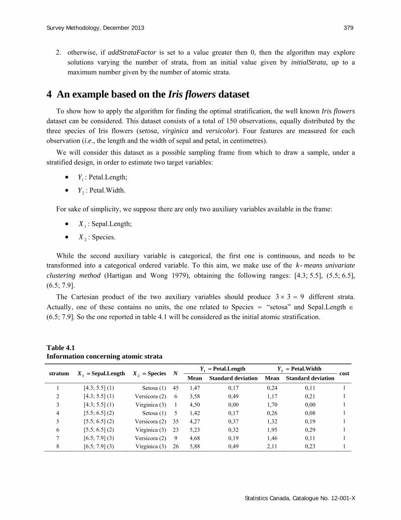
4 An example based on the Iris flowers dataset

To show how to apply the algorithm for finding the optimal stratification, the well known Iris flowers dataset can be considered. This dataset consists of a total of 150 observations, equally distributed by the three species of Iris flowers (setosa, virginica and versicolor). Four features are measured for each observation (i.e., the length and the width of sepal and petal, in centimetres).

We will consider this dataset as a possible sampling frame from which to draw a sample, under a stratified design, in order to estimate two target variables:

1Y : Petal.Length;

2Y : Petal.Width.

For sake of simplicity, we suppose there are only two auxiliary variables available in the frame:

1X : Sepal.Length;

2X : Species.

While the second auxiliary variable is categorical, the first one is continuous, and needs to be transformed into a categorical ordered variable. To this aim, we make use of the k- means univariate

clustering method (Hartigan and Wong 1979), obtaining the following ranges: [4.3; 5.5], (5.5; 6.5], (6.5; 7.9].

The Cartesian product of the two auxiliary variables should produce 3 3 9 different strata.

Actually, one of these contains no units, the one related to Species “setosa” and Sepal.Length (6.5; 7.9]. So the one reported in table 4.1 will be considered as the initial atomic stratification.

Table 4.1 Information concerning atomic strata

stratum 1X Sepal.Length 2X Species N 1Y Petal.Length 2Y Petal.Width cost

Mean Standard deviation Mean Standard deviation

1 [4.3; 5.5] (1) Setosa (1) 45 1,47 0,17 0,24 0,11 1

2 [4.3; 5.5] (1) Versicora (2) 6 3,58 0,49 1,17 0,21 1

3 [4.3; 5.5] (1) Virginica (3) 1 4,50 0,00 1,70 0,00 1

4 [5.5; 6.5] (2) Setosa (1) 5 1,42 0,17 0,26 0,08 1

5 [5.5; 6.5] (2) Versicora (2) 35 4,27 0,37 1,32 0,19 1

6 [5.5; 6.5] (2) Virginica (3) 23 5,23 0,32 1,95 0,29 1

7 [6.5; 7.9] (3) Versicora (2) 9 4,68 0,19 1,46 0,11 1

8 [6.5; 7.9] (3) Virginica (3) 26 5,88 0,49 2,11 0,23 1



For sake of simplicity, we assume that the fixed cost 0C is null, and all hC are set equal to 1: by so

doing, the cost of a solution coincides with the sum of sampling units allocated in the strata, i.e., with the

total sample size 1.

H

hhC n n

We set as precision constraints to the estimates of both target variables an upper limit of 0.05 (5%) to their expected coefficient of variation.

Finally, we set a minimum number of units to be selected in each stratum equal to 2 (the minimum required in order to calculate sampling variance).

Under these assumptions, and using the atomic stratification, the Bethel algorithm solves the optimal allocation problem by defining a minimum sample size of 17 units, with an allocation vector

2, 2,1, 2, 3, 3, 2, 2 .a

If we proceed to partition the set of atomic strata, the resulting number of all possible stratifications (given by the Bell formula) is 8B 4,140. This number is such that we can afford to enumerate all

partitions of atomic strata, and for each of them we are able to calculate the minimum sample size by applying the Bethel algorithm (to enumerate all the partitions in this example, we made use of the function setparts(), contained in the R package partitions (Hankin 2011)).

The range of sample sizes steps from a minimum of 11 to a maximum of 78 (this latter corresponds to the “no stratification solution”) (see figure 4.1).

We notice that the minimum value 11n that has been found is considerably lower than the one

calculated in correspondence with the atomic stratification 17 .n This minimum value characterizes

only 8 partitions out of 4,140.

Now, the genetic algorithm is applied in order to evaluate its capability to find the optimal solution (or at least one that is not far from it), without being obliged to explore all solutions, but only a strict subset of them.

Figure 4.1 Space of partitions

Space of partitions Histogram of partitions

0 1,000 3,000 10 30 50 70 Partitions Sample size required

Sam

ple

size

req

uire

d 10

2

0

30

4

0

50

6

0

70

8

0

Fre

quen

cy o

f pa

rtit

ions

1

0

10

0

20

0

30

0

400

500



Step 0: Creation of the initial generation

First, we set 8U (we can accept a number of final strata that is equal to the number of atomic strata, so U K ). The generation size parameter pop is set equal to 10. So, an initial set containing 10 different

individuals (stratifications) is generated. Each of them is represented by a vector of 8 elements, i.e., the number of different atomic strata. An individual 1, 2, 3, 4, 5, 6, 7, 8v or, equivalently,

3, 6, 4, 2,1, 8, 7, 5v corresponds to the most detailed stratification (as all strata are labelled with

different labels), while 1,1,1,1,1,1,1,1v or equivalently 4, 4, 4, 4, 4, 4, 4, 4v corresponds to

“null stratification” (as atomic strata are labelled with identical labels). Step 1: Evaluation of fitness for each individual in the generation

To each one of the 10 individuals in the current generation, the Bethel algorithm is applied in order to find the cost of the sample required to comply with fixed precision constraints.

To do this, first of all related strata and information are calculated for each individual. For example, for a generated individual 4,1,1, 4, 8, 7, 8,1v the information is derived by the one available from atomic

strata, by applying (3.1) and (3.2) (see table 4.2).

Table 4.2 Information concerning generated aggregated strata

Aggregated stratum

Original atomic strata

1 2,X X N1Y 2Y

Mean Standard deviation Mean

Standard deviation

1 2,3,8 (1,2) or (1,3) or (3,3) 33 5.41 1.01 1.92 0.44

2 1,4 (1,1) or (2,1) 50 1.46 0.17 0.25 0.10

3 6 (2,3) 23 5.23 0.31 1.95 0.28

4 5,7 (2,2) or (3,2) 44 4.35 0.37 1.35 0.18

The fitness of this individual is measured by the corresponding required sample size, that results to be 14, with an allocation vector 6, 2, 3, 3 .a

All individuals are sorted accordingly with their performance: the individual in the first position is the one supporting the minimum sample size, the 10th individual is the one requiring the maximum sample size. Step 2: Breeding a new generation

By setting the elitism parameter to 20% (a common default value) we always take the best 2 individuals in the current generation and directly move them to the next generation, without any change of their genome.



Then, we proceed in generating new individuals in the following way:

1. we select couples of individuals of the current generation with probability proportional to their fitness: for instance, assume to select v 1,1, 3, 4, 3, 2, 2, 2k and v 2, 2, 2, 2, 2,1,1,1 ;j

2. a crossover point is randomly generated, i.e., an integer internal to the interval 1, 8 : suppose to

set it equal to 3; 3. the crossover is performed by assigning to the child the first three elements of parent v k and the

last five elements of parent v ,j obtaining in this way newv 1,1, 3, 2, 2,1,1,1 ;

4. having set a mutation rate parameter equal to 0.05, for each element of the child a random number is generated in the interval 0,1 : if it is less than 0.05, the value of the element is changed (by

generating a new value comprised between 1 and 9), otherwise it is not changed. Step 3: Iteration and stopping criteria

The number of iterations has been set equal to 25. So, steps 1 and 2 are repeated 25 times. The individual with the best fitness alongside all the generations is retained as the best solution.

The graph in figure 4.2, obtained during the execution of the program, shows the convergence of the algorithm. In the graph, two different curves are reported: the lower one is related to the best solution found until the thk iteration (as the best solution is memorised, it can only decrease as the algorithm

proceeds); the upper one reports the mean of the 10 solutions evaluated in each iteration.

Figure 4.2 Best and mean evaluation values during GA execution

The resulting best solution is 4,1, 3, 4,1, 3, 3, 2 .v It corresponds to the stratification reported in

table 4.3, with an allocation vector 3, 2, 4, 2 .a

5 10 15 20 25 Iteration (Generation)

Bes

t (bl

ack

low

er li

ne)

and

mea

n

(red

upp

er li

ne)

eval

uati

on v

alue

15

2

0

25

3

0

Domain 1 – Sample size 11



Table 4.3 Information concerning final strata

Aggregated stratum

Original atomic strata

1 2,X X N1Y 2Y

Mean Standard deviation

Mean Standard deviation

1 2,5 (1,2) or (2,2) 41 4.16 0.45 1.30 0.19

2 8 (3,3) 26 5.88 0.49 2.10 0.22

3 3,6,7 (1,3) or (2,3) or (3,2) 33 5.06 0.38 1.80 0.33

4 1,4 (1,1) or (2,1) 50 1.46 0.17 0.25 0.10

In conclusion, by applying the genetic algorithm, we succeeded in finding the optimal solution by exploring only 25 10 250 alternative stratifications instead of the 4,140 belonging to the universe of

partitions.

In order to verify that this result is not due to a “lucky strike”, we perform different executions of the algorithm: each execution iterates 10 times the application of the genetic algorithm, varying the values of the parameter “number of iterations”. Results are reported in table 4.4.

Table 4.4 Capability of GA to find the optimal solution

Execution of the GA

(10 times each)

Value of parameter “number of

iterations” in the GA

Solutions with n = 11

(optimal)

Solutions with

n = 12

Solutions with

n = 14

(a) 25 5 4 1

(b) 50 7 3 -

(c) 100 9 1 -

(d) 200 10 - -

In execution (a), we discover that, with only 25 iterations, to succeed in finding the optimal solution is actually a “lucky strike”, as in half of the trials the found solution is higher than the optimal. But increasing the number of the iterations up to 200 (execution (d)), the genetic algorithm proves to be reliable with respect to its capability to reach optimality, as in all the trials the optimal solution is found.

As for the number of the strata corresponding to the found optimal solutions, on average it is 4, with a range of 3, 5 .

Finally, we also want to verify that the found solutions are compliant with the precision constraints (maximum CV equal to 5% for both target variables). So, in execution (d) (iterations 200 ), for each

one of the 10 produced solutions we proceed to draw 1,000 samples from the frame and to calculate the related CV’s. Corresponding results are shown in figure 4.3: the average of CV’s for the first target variable (Petal.Lenght) is around 3%, while for the second one is around 5%. So, we can say that, on average, precision constraints have not been violated.



Figure 4.3 Distributions of CV’s for target variables in the simulation

A more complete example involving the use of all the functions in the package SamplingStrata is

reported in Barcaroli (2013b).

5 An application: the Italian Farm Structure Survey (FSS)

The sampling frame used for the selection of 2003 Italian Farm Structure Survey (FSS) sample contains 2,153,710 farms. For the purposes of FSS sample design, the auxiliary variables considered are the following:

1. regions (21 different values); 2. provinces (103 different values); 3. legal status (2 classes); 4. sector of economic activity (9 classes); 5. economic size unit (3 classes); 6. agricultural area utilized (3 classes); 7. livestock unit (3 classes); 8. altimetry of the headquarter of the holding (5 classes).

Fourteen different target variables have been considered as the main target of FSS, on which the required precision levels (in terms of maximum coefficient of variations) have been fixed at regional level (domains of interest). The list of variables and related precision constraints are reported in table 5.1.

1 2 3 4 5 6 7 8 9 10 1 2 3 4 5 6 7 8 9 10 Executions of GA (1-10) Executions of GA (1-10)

CV

%

1

2

3

4

5

6

7

CV

%

2

4

6

8

1

0

CV1 CV2



Both the 8 auxiliary and the 14 target variables have been observed during the previous 2000 Agricultural Census, so their values are available for each unit in the frame. This gives the possibility to calculate means and standard deviations related to whichever defined stratum.

Firstly, the current “manual” procedure followed in 2003 to choose the most suitable stratification for sample selection is described. 2003 manual configuration of strata to select the FSS sample

In the first step, a take-all stratum was defined in each region on the basis of local characteristics. The thresholds for defining the take-all strata were determined using the Hidiroglou method (1986).

In the second step, a choice between a stratification based on provinces or on the region as a whole, was chosen region by region, on the basis of local organizational considerations.

In the third step, the other six variables were alternatively used in each region or provinces (depending on the result obtained in the second step) as stratification variables. For each of such alternative stratifications, the optimal sample size was computed (the minimum sample size in each stratum had been fixed to 50) (in the cost function, fixed cost has been set to zero, and variable costs were set equal to 1 in each atomic stratum: so the cost function coincides with the total sample size). The stratification supporting the overall minimum sample size in each region (usually defined on different variables) was considered as the output of this step.

In the fourth step, the remaining five variables were used separately to refine the stratification previously obtained. For each of these refined stratifications the optimal sample size was computed considering the same constraints used in the third step.

This stepwise procedure was repeated on a regional basis, by refining the best stratification obtained in each step, using the remaining available variables until the obtained stratification revealed to be less efficient than the stratification in the previous step.

By so doing, the total amount of planned sample size was fixed to 42,465 units (actually, the sample size used for 2003 FSS was increased to 52,713 in order to obtain better estimates at national level. Here we consider the number of 42,465 to correctly compare the results obtained with the genetic algorithm). Use of the genetic algorithm to identify optimal strata and best allocation

The most detailed available stratification of the frame, obtained as a Cartesian product of all the auxiliary variables, consists of 24,454 different strata, 1,787 of which have been defined as take-all strata. So, the atomic strata are given by the 22,667 sampling strata obtained by subtracting the 1,787 take-all strata. The latter are collapsed in only one stratum, whose 6,971 units will always be selected for whatever sample.

Actually, one of the auxiliary variables, region, is considered as the domain variable. So, our task consists in optimising the frame stratification and the sample allocation distinctly for each one of the different 21 Italian regions. For instance, the first region (Piemonte) is characterised by 105,074 units in 1,646 sampling strata, and 597 units in 129 take-all strata.

Precision constraints (once again expressed in terms of upper limits on coefficients of variation) have been set, for each one of the 14 different target variables, at the same values chosen on the occasion of



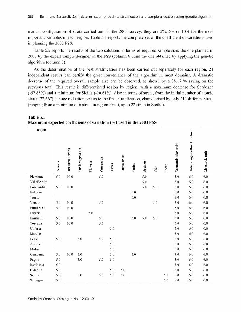
manual configuration of strata carried out for the 2003 survey: they are 5%, 6% or 10% for the most important variables in each region. Table 5.1 reports the complete set of the coefficient of variations used in planning the 2003 FSS.

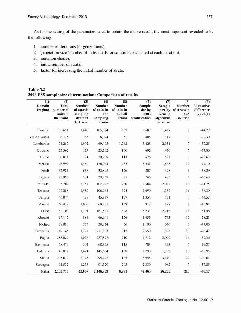
Table 5.2 reports the results of the two solutions in terms of required sample size: the one planned in 2003 by the expert sample designer of the FSS (column 6), and the one obtained by applying the genetic algorithm (column 7).

As the determination of the best stratification has been carried out separately for each region, 21 independent results can certify the great convenience of the algorithm in most domains. A dramatic decrease of the required overall sample size can be observed, as shown by a 38.17 % saving on the previous total. This result is differentiated region by region, with a maximum decrease for Sardegna (-57.85%) and a minimum for Sicilia (-20.61%). Also in terms of strata, from the initial number of atomic strata (22,667), a huge reduction occurs to the final stratification, characterised by only 213 different strata (ranging from a minimum of 6 strata in region Friuli, up to 22 strata in Sicilia). Table 5.1 Maximum expected coefficients of variation (%) used in the 2003 FSS

Region

Cer

eals

Ind

ustr

ial c

rops

Fre

sh v

eget

able

s

Flo

wer

s

Vin

eyar

ds

Oli

ves

Cit

rus

fru

it

Fru

its

Bov

ines

Pig

s

Shee

p

Eco

nom

ic s

ize

un

its

Uti

lize

d a

gric

ult

ura

l su

rfac

e

Liv

esto

ck u

nit

Piemonte 5.0 10.0 5.0 5.0 5.0 6.0 6.0

Val d’Aosta 5.0 5.0 6.0 6.0

Lombardia 5.0 10.0 5.0 5.0 5.0 6.0 6.0

Bolzano 5.0 5.0 6.0 6.0

Trento 5.0 5.0 6.0 6.0

Veneto 5.0 10.0 5.0 5.0 5.0 6.0 6.0

Friuli V.G. 5.0 10.0 5.0 6.0 6.0

Liguria 5.0 5.0 6.0 6.0

Emilia R. 5.0 10.0 5.0 5.0 5.0 5.0 5.0 6.0 6.0

Toscana 5.0 10.0 5.0 5.0 6.0 6.0

Umbria 5.0 5.0 6.0 6.0

Marche 5.0 6.0 6.0

Lazio 5.0 5.0 5.0 5.0 5.0 6.0 6.0

Abruzzi 5.0 5.0 6.0 6.0

Molise 5.0 5.0 6.0 6.0

Campania 5.0 10.0 5.0 5.0 5.0 5.0 6.0 6.0

Puglia 5.0 5.0 5.0 5.0 5.0 6.0 6.0

Basilicata 5.0 5.0 6.0 6.0

Calabria 5.0 5.0 5.0 5.0 6.0 6.0

Sicilia 5.0 5.0 5.0 5.0 5.0 5.0 5.0 6.0 6.0

Sardegna 5.0 5.0 5.0 6.0 6.0



As for the setting of the parameters used to obtain the above result, the most important revealed to be the following:

1. number of iterations (or generations); 2. generation size (number of individuals, or solutions, evaluated at each iteration); 3. mutation chance; 4. initial number of strata; 5. factor for increasing the initial number of strata.

Table 5.2 2003 FSS sample size determination: Comparison of results

(1) Domain (region)

(2) Total

number of units in

the frame

(3) Number

of atomic sampling strata in

the frame

(4)Number

of units in the

sampling strata

(5)Number

of units in take-all

strata

(6)Sample size by

2003 stratification

(7) Sample size by

Genetic Algorithm

solution

(8) Number

of strata in GA

solution

(9)% relative difference

(7) vs (6)

Piemonte 105,671 1,646 105,074 597 2,687 1,497 9 -44.29

Valle d’Aosta 6,125 65 6,074 51 408 317 7 -22.30

Lombardia 71,257 1,902 69,495 1,762 3,428 2,151 7 -37.25

Bolzano 23,362 127 23,202 160 692 430 7 -37.86

Trento 30,021 124 29,908 113 676 523 7 -22.63

Veneto 176,999 1,450 176,064 935 3,531 1,868 11 -47.10

Friuli 32,981 638 32,805 176 807 498 6 -38.29

Liguria 29,992 584 29,967 25 766 485 7 -36.68

Emilia R. 103,702 2,157 102,922 780 2,584 2,022 11 -21.75

Toscana 107,288 1,959 106,964 324 2,099 1,337 16 -36.30

Umbria 46,074 435 45,897 177 1,354 751 7 -44.53

Marche 60,439 1,005 60,271 168 918 488 8 -46.84

Lazio 162,109 1,304 161,801 308 3,233 2,216 14 -31.46

Abruzzi 67,117 888 66,941 176 1,035 743 10 -28.21

Molise 28,890 375 28,834 56 1,190 630 6 -47.06

Campania 212,145 1,271 211,833 312 2,559 1,883 13 -26.42

Puglia 288,087 1,026 287,877 210 4,712 2,009 14 -57.36

Basilicata 68,470 504 68,355 115 703 493 7 -29.87

Calabria 145,812 1,624 145,654 158 2,798 1,792 17 -35.95

Sicilia 295,637 2,345 295,472 165 3,955 3,140 22 -20.61

Sardegna 91,532 1,238 91,329 203 2,330 982 7 -57.85

Italia 2,153,710 22,667 2,146,739 6,971 42,465 26,255 213 -38.17



Their final values have been determined, after numerous trials, on the basis of the analysis of the runs for each region.

In particular, by inspecting the convergence plot, it is possible to understand if the number of iterations is sufficient to ensure that the final solution is definitely the best obtainable, or if otherwise a higher number of iterations is needed. This can be done by analysing the behaviour of the two curves in the plot: the lower one reports the best evaluation value, while the upper one refers to the mean evaluation value. When the mean evaluation value is still decreasing, together with the best evaluation value, it is worthwhile to go on iterating. When the best value line becomes stably constant (and typically the mean value line begins to fluctuate up and down), no further gain can be expected by new iterations. This is the case, for instance, of the convergence plot for Trento region, shown in figure 5.1.

A convenient value for iterations parameter was found to be 5,000. As for the mutation chance, a suitable value was found to be 0.001: this means that, for any chromosome in the genome (any value in vector v ), a mutation occurred on average only once out of a thousand. A critical point is in fixing the

initial number of strata. Since the final solution is very sensitive on the number of strata, we decided to let the algorithm to choose it. This can be done, as already said in section 4, by assigning a low value to initialStrata, and by giving a value greater than zero to addStrataFactor: this enables the algorithm to explore solutions characterized by a wide range of number of strata. In our experiment, we set the initial number of strata to the value 5, while assigning a value 0.01 to the factor for increasing the initial number of strata (this means that, any time a mutation occurs, there is a probability of 1% to increase by 1 the current number of strata).

Figure 5.1 Best and mean evaluation value for the Trento region

From a computational point of view, the overall task required an elapsed time of 641,820 seconds (more than 178 hours, nearly one week) (the job was run on a desktop AMD Athlon 64 2 (2.90 Ghz,

3 GB RAM)).

0 1,000 2,000 3,000 4,000 5,000 Iteration (Generation)

Bes

t (bl

ack

low

er li

ne)

and

mea

n (r

ed u

pper

line

) ev

alua

tion

val

ue

1,0

00

2

,000

3,0

00

4

,000

5,0

00




6 A further application: the Monthly survey on milk and milk products

A further application of our algorithm concerned the 2010 Monthly survey on milk and milk products. This is a sample survey that depends strictly on the “Annual survey on milk and milk products”, which is a census of all Italian farms producing milk and milk products. Both surveys collect the same information: the amount of milk collected at the national level and its use (in processing dairy products: milk, cheese, butter, etc.); the purpose of the monthly sample survey is to obtain timely information before the results of the annual survey (carried out in the year before) become available. The sample for 2010 has been planned in this way:

1. the information collected on the 2,250 respondent units in the 2008 round of the Annual survey were organised as a frame: in particular, four of the target variables of the Annual survey, which are continuous, were transformed into categorical variables (ordered factors) by using the k- means

clustering method, and considered as auxiliary information in the frame; 2. the cross-product of the obtained categorical variables, produced a stratification of the frame

consisting in 152 (atomic) strata; 3. the information related to means and standard deviations of the four target variables of the monthly

survey were calculated for each one of the atomic strata by using Annual survey data.

Constraints on the coefficients of variation of the estimates of the totals are reported in table 6.1.

Table 6.1 Coefficients of variation (%) used in planning the 2010 Monthly Survey on Milk

Variable Maximum acceptable CV on total estimates (%)

Collected milk 1Milk 15Butter 3.8Cow’s milk cheeses 3

After this, the Bethel algorithm was applied in order to verify the sample size required with the initial (atomic) stratification available for the frame (also in this application, the function cost coincides with the total sample size, as the fixed cost was set to zero, and variable costs were set equal to 1 in each atomic stratum): it resulted in 290 units to be interviewed, allocated in the 152 different strata. The usual procedure terminates here: at this point, the 290 units would be selected from the frame represented by the Annual Survey, and the Monthly Survey would start.

Instead, the application of the genetic algorithm suggested a collapsing of the 152 initial atomic strata into 88 aggregate strata, requiring a sample size of only 247 to satisfy the same constraints, with a consequent decrease of about 15%.



After a considerable amount of attempts, the following values were given to the most important parameters:

1. generation size was set equal to 50; 2. the number of iterations was set equal to 4,000; 3. a minimum of 2 units per stratum was required; 4. the initial number of strata (coinciding with the maximum number of them, as parameter

addStrataFactor was set to 0) was set equal to the number of atomic strata (152); 5. the mutation chance was set to 0.0005.

The combination of parameter “generation size” and “number of iterations” determined the evaluation of 200,000 50 4,000 solutions. The convergence plot reported in figure 6.1 shows that after

2,700/2,800 there has been no further improvement of the identified best solution.

Figure 6.1 Best and mean evaluation value in the optimization of Monthly Survey on Milk

7 Conclusions and future work

For any given multipurpose and multidomain sample survey, the optimal stratification of the sampling frame can be determined together with the optimal sample size and allocation of units among strata, by means of a combined use of the Bethel algorithm (or, more generally, of a NLP solver) for the determination of the minimum sample size required to satisfy precision constraints, and of the genetic algorithm for the exploration of the universe of potential stratifications, rigorously generated accordingly to the theory of partitions. The information required is nearly the same as the one required by the allocation problem: desired precision on estimates of total (or means) of target variables, and information

0 1,000 2,000 3,000 4,000 Iteration (Generation) B

est (

blac

k lo

wer

line

) an

d m

ean

(red

upp

er li

ne)

eval

uati

on v

alue

30

0

40

0

500

600

700




regarding the distributions of each target variable in population strata. Initial stratification should be considered at the most detailed level (atomic stratification), i.e. the one determined by the Cartesian product of values of all available stratification variables.

The complete exploration of the set of all possible stratifications is in practical cases computationally prohibitive. The use of the genetic algorithm permits to explore the space of solutions in a very efficient manner. By carefully tuning the execution parameters, it is possible to determine the optimal solution, or at least a solution likely to be not far from the optimal one.

The application of this algorithm to two different surveys (the 2003 Italian Farm Structure Survey and the 2010 Monthly milk and milk products) shows that the obtained solutions are much better, in terms of sample efficiency, than the ones manually produced by expert methodologists (in Istat, the algorithm has been applied to three more surveys: “Economic outcomes of agricultural holdings”, “Structure and production of main wooden cultivations”, “Survey on forecasting of some herbal crops sowing”).

In all the cases reported, it has been possible to calculate the values required as input to our algorithm (in particular: means and standard deviations of the target variables in the different atomic strata), because of the availability of related values for each unit in the frames. In more realistic situations, this kind of information is not directly available. Instead, we could use estimates produced by alternative sources: administrative data, other surveys, or previous rounds of the same survey, or even hypothesis (usually conservative) on the variability of target variables within the strata. Accordingly to Rivest (2002) it is also possible to model target variables assuming auxiliary variables ’X s as explanatory variables, in order to estimate means and standard deviations on the basis of predicted values of ’Y s. Of course, the less “direct” is the information on the target variables, the less robust is the proposed method, because of the uncertainty caused by the use of proxy information, or model-based predictions.

Another limit affecting this approach still lies in the handling of continuous auxiliary variables. In our approach, we simply suggest to transform them into categorical ones, in order to be considered in the determination of the universe of all possible stratifications of the sampling frame. A first element for future work is in giving indications on how to transform these variables in order to get the best from them. A second one is in the fact that some of the strata contained in the optimal solution may be characterized by non contiguous values of the transformed continuous variables, or of the categorical ordinal variables, which is something odd that should not be allowed: this could be prevented by imposing constraints on the generation of candidate solutions.

References

Baillargeon, S., and Rivest, L.-P. (2009). A general algorithm for univariate stratification. International Statistical Review, 77, 3, 331-344.

Baillargeon, S., and Rivest, L.-P. (2011). The construction of stratified designs in R with the package

stratification. Survey Methodology, 37, 1, 53-65. Barcaroli, G., Pagliuca, D. and Willighagen, E. (2013a). SamplingStrata: Optimal stratification of

sampling frames for multipurpose sampling surveys. R package version 1.0-1. http://cran.r-project.org/web/packages/SamplingStrata/index.html.



Barcaroli, G. (2013b). Optimization of sampling strata with the SamplingStrata package. http://cran.r-project.org/web/packages/SamplingStrata/vignettes/SamplingStrataVignette.pdf.

Benedetti, R., Espa, G. and Lafratta, G. (2008). A tree-based approach to forming strata in multipurpose

business surveys. Survey Methodology, 34, 2, 195-203. Bethel, J. (1985). An optimum allocation algorithm for multivariate surveys. American Statistical

Proceedings of the Survey Research Methods Section, 209-212. Bethel, J. (1989). Sample allocation in multivariate surveys. Survey Methodology, 15, 1, 47-57. Chromy, J.B. (1987). Design optimization with multiple objectives. Proceedings of the American

Statistical Association Section on Survey Research Methods 1987, 194-199. Cochran, W.G. (1977). Sampling Techniques. New York: John Wiley & Sons, Inc. Dalenius, T., and Hodges, J.L. (1959). Minimum variance stratification. Journal of American Statistical

Association, 54, 88-101. Day, C.D. (2006). Application of an evolutionary algorithm to multivariate optimal allocation in stratified

sampling designs. Proceedings of the American Statistical Association Section on Survey Research Methods 2006 [CD-ROM].

Day, C.D. (2010). A multi-objective evolutionary algorithm for multivariate optimal allocation. Section on

Survey Research Methods - JSM 2010, 3351-3358. Díaz-García, J.A., and Cortez, L.U. (2008). Multi-objective optimisation for optimum allocation in

multivariate stratified sampling. Survey Methodology, 34, 2, 215-222. Gunning, P., and Horgan, J.M. (2004). A new algorithm for the construction of stratum boundaries in

skewed populations. Survey Methodology, 30, 2, 159-166. Hankin, R.K.S., and West, L.J. (2007). Set Partitions in R. Journal Of Statistical Software, Code Snippet

2. December 2007, 23, http://www.jstatsoft.org/. Hankin, R.K.S. (2011). Partitions: Additive partitions of integers. R package version 1.9-19. http://cran.r-

project.org/web/packages/partitions/index.html. Hartigan, J.A., and Wong, M.A. (1979). A k-means clustering algorithm. Applied Statistics, 28, 100-108. Hidiroglou, M.A. (1986). The costruction of self-representing stratum of large units in survey design. The

American Statistician, 40, 27-31. Huddleston, H.F., Claypool, P.L. and Hocking, R.R. (1970). Optimal sample allocation to strata using

convex programming. Applied Statistics, 19, 273-278. Keskintürk, T., and Er, S. (2007). A genetic algorithm approach to determine stratum boundaries and

sample sizes of each stratum in stratified sampling. Computational Statistics and Data Analysis, 15 September 2007, 52, 1, 53-67.



Khan, M.G.M., Nand, N. and Ahmad, N. (2008). Determining the optimum strata boundary points using dynamic programming. Survey Methodology, 34, 2, 205-214.

Khan, M.G.M., Maiti, T. and Ahsan, M.J. (2010). An optimal multivariate stratified sampling design using

auxiliary information: An integer solution using goal programming approach. Journal of Official Statistics, 26, 4, 695-708.

Kish, L. (1976). Optima and proxima in linear sample designs. Journal of the Royal Statistical Society,

Series A, 159, 80-95. Kozak, M., Verma, M.R. and Zieliński, A. (2007). Modern approach to optimum stratification: Review

and perspectives. Statistics in Transition, 8(2), 223-250. Kozak, M., Zieliński, A. and Singh, S. (2008). Stratified two-stage sampling in domains: Sample

allocation between domains, strata, and sampling stages. Statistics & Probability Letter, June 2008, 78, 8, 970-974.

Kozak, M., and Wang, H.Y. (2010). On stochastic optimization in sample allocation among strata.

Metron - International Journal of Statistics, LXVIII, 1, 95-103. Lavallée, P., and Hidiroglou, M.A. (1988). On the stratification of skewed populations. Survey

Methodology, 14, 1, 33-43. Rivest, L.-P. (2002). A generalization of the Lavallée and Hidiroglou algorithm for stratification in

business surveys. Survey Methodology, 28, 2, 191-198. Schmitt, L.M. (2001). Theory of genetic algorithms. Theoretical Computer Science, 259, 1-61. Schmitt, L.M. (2004). Theory of genetic algorithms II: Models for genetic operators over the string-tensor

representation of populations and convergence to global optima for arbitrary fitness function under scaling. Theoretical Computer Science, 310, 181-231.

Singh, R. (1971). Approximately optimum stratification on the auxiliary variables. Journal of the

American Statistical Association, 66, 829-833. Stokes, L., and Plummer, J. (2004). Using spreadsheet solvers in sample design. Computational Statistics

& Data Analysis, 44, 527-546. Vose, M.D. (1999). The Simple Genetic Algorithm: Foundations and Theory, MIT Press, Cambridge,

MA. Willighagen, E. (2012). Genalg: R Based Genetic Algorithm. R package version 0.1.1. http://cran.r-

project.org/web/packages/genalg/index.html.

joint determination of optimal stratification and sample allocation …€¦ · ·...

Documents